Analytical Ultracentrifugation of Polymers and Nanoparticles (Springer Laboratory)

;XZQVOMZ4IJWZI\WZa

;XZQVOMZ4IJWZI\WZa5IV]IT[QV8WTaUMZ;KQMVKM 8I[KPMZTIO*MZTQV0MQLMTJMZO 8ZQV\MLQV/MZUIVa 0), the intersection point of a monodisperse

Fig. 3.7. Typical van Holde-Weischet plot for the elimination of diffusion broadening in a sedimentation velocity experiment with dissolved monodisperse macromolecules at one concentration (reprinted with permission from [45])

60

3 Sedimentation Velocity

component is shifted to times less than infinity, i.e., to negative values of t −0.5 . Therefore, the van Holde-Weischet analysis is also a test for sample homogeneity and/or non-ideality. The interpretation of van Holde-Weischet diagrams becomes complicated in the case of a broad continuous distribution of components, for non-ideality, and for very small particles. In Sect. 3.4.2 and Fig. 3.11, a modified van Holde-Weischet procedure [2] is described for the separation of diffusion and polydispersity broadening. Time Derivative Method In many cases, samples show either multiple components or even a continuous distribution of particle sizes or molar masses. In such cases, it is of interest to determine the diffusion-corrected sedimentation coefficient distribution as mentioned above in the form of G(s), or in the differential form thereof, g(s). Although this is in principle possible by the van Holde-Weischet method, a more suitable method for the determination of g(s) is the time derivative method ([17]; see also [1]). It determines the time derivative of neighboring radial scans – J(r, t), A(r, t) or c(r, t) – acquired at different times t according to (3.10), which is a combination of (3.2) and (3.3): g ∗ (s)t

=



∂ {c(r, t)/c0 } ∂t



ω2 t 2 ln(rm /r)



r rm

2

=

∂G∗ (s)t ∂s

(3.10)

with g ∗ (s) being the apparent s distribution. The star indicates that this distribution is not diffusion-corrected. The apparent g ∗ (s) distribution equals the true distribution g(s) in cases where diffusion can be ignored. To eliminate the influence of a significant diffusion broadening, an extrapolation of the different g(s∗ , t) curves, calculated for different times t to infinite time t = ∞, yields the true distribution g(s). An important advantage of the time derivative procedure is a significant improvement of the quality of the calculated distribution g ∗ (s)t , because two neighboring scans are subtracted from each other, so that systematic errors in the optical patterns (baseline, window distortion, etc.) are removed and the random noise decreases. As a drawback, it has to be noted that only scans from a relatively narrow time interval can be used for a single g ∗ (s) evaluation, because the time derivative method fails for very broadly distributed samples. It works, however, very well for moderately distributed samples exhibiting two plateaus in every scan, one on the left and one on the right of the sedimentation boundary. Figure 7.6 in Sect. 7.3 is an illustration of the above. It shows diffusion-broadened UV optics scans A(r, t) of a sedimentation velocity run of small, moderately distributed gold (colloid) particles, which are evaluated with three different methods: (i) with the simple procedure of (3.2), (ii) with the time derivative methods of (3.10), yielding the non-diffusion-corrected g ∗ (s) distribution, and (iii) with a diffusion correction

3.3 Advanced Theory of Sedimentation Velocity Runs

61

to transform g ∗ (s) into g(s), using the method of Schuck [18] described in the following section. Lamm Equation Modeling Very recently, Schuck [18] published a new approach for the analysis of AUC sedimentation data. By modeling of the Lamm equation (1.10), now even sedimentation coefficients and molar mass distributions of polydisperse samples can be investigated. The principle of this approach is based on an educated initial guess of the sedimentation coefficients, the frictional coefficients, and the partial specific volume of the sample. This guess is utilized to calculate finite element solutions for a large number of discrete virtual species with different s values. The calculated data are adjusted to the experimental data by means of maximum entropy regularization, yielding a continuous sedimentation coefficient distribution g(s). This approach offers an easy access to diffusion-corrected sedimentation coefficient distributions g(s) [19]. A drawback of Schuck’s method are the essentially non-existing “ghost peaks” in very broad distributions (for practical examples, see Fig. 7.6 and [20]). 3.3.7 Test of Homogeneity Often, the question arises whether an examined sample is really homogenous. Attention has to be paid if data from AUC sedimentation velocity runs are applied to answer this question. There are several criteria allowing statements on homogeneity of a sample preparation. It must be kept in mind that homogeneity can only be presumed through the absence of detectable heterogeneity. Two important criteria are the following. Criteria of boundary shape and broadening There must be a single symmetrical boundary throughout the duration of the sedimentation velocity experiment, such as, for example, in Figs. 3.1 and 3.2. As mentioned in Sect. 3.3.6, it is possible to separate the influence of diffusion on the broadening of a boundary from the influence of heterogeneity. Criteria of Mass Conservation The measurable boundary, a step-like A(r) or J(r) scan or a Schlieren peak area, must account for all the material put into the cell, after corrections for radial dilution, throughout the duration of the sedimentation velocity experiment. Depending on the applied detecting system, either the specific decadic extinction coefficient ε or the specific refractive index increment (dn/dc)p has to be known to allow the exact evaluation of mass conversation. If the plateau concentration cp near the cell bottom does not reflect the initial concentration c0 (after correction for the abovementioned effects), heavy and/or large particles may have already settled very fast (in a non-detectable manner) at the bottom of the cell. This is definitely an indication of heterogeneity.

62

3 Sedimentation Velocity

3.4 Sedimentation Velocity Runs of Macromolecules to Measure Average M and MMD In the first sections of this Chap. 3, we introduced the technique of sedimentation velocity runs, the basic ideas, but also some limitations and pitfalls. Now, we will use this technique to measure average molar masses M and molar mass distributions (MMD) of dissolved macromolecules. Besides measurements of PSD (see Sect. 3.5), measurements of MMD are the second most important industrial task of the AUC. To carry out MMD measurements, we need a relation between the desired M and the measured sedimentation coefficient s, in analogy to that of (1.9) for the determination of particle diameters dp via s measurements. Equation (1.8) is a relation between M and s, but we cannot use it to determine M via s runs because it requires additionally the knowledge of the (normally) unknown diffusion coefficient D of the solute. Thus, we have to look for another M(s) relation. This is an empirical scaling law in the form: s0

= K · Ma

(3.11)

where s0 is the sedimentation coefficient at infinite dilution c → 0, and K and a are the (constant) scaling parameters, valid for the respective homologs of a (special) polymer, in a (special) solvent at a defined temperature T. If one changes the polymer, the solvent or the temperature, also the scaling parameters K and a will be changed. In analogy to the parameter b in (3.9), the parameter a depends on the shape of the dissolved macromolecules and the solvent/solute interactions, too. Typical numerical values of a are 0.2 < a ≤ 0.5 (according to Svedbergs’ Eq. (1.8), a + b = 1 should be valid). In Sect. 3.4.1, we will show how it is possible to derive such a scaling law, using a series of (nearly) monodisperse samples (or fractions) of a polymer. In Sect. 3.4.2, we will then use such a scaling law to measure a complete MMD of a broadly distributed polymer via s runs, and practice at the same time the radial dilution correction discussed above in Sect. 3.2.3, the concentration dependence correction in Sect. 3.2.4, and the diffusion correction in Sect. 3.3.6. 3.4.1 Evaluation of the Average Molar Mass M by Sedimentation Velocity Runs via Scaling Laws Sedimentation velocity runs can be used to measure the molar mass M of (synthetic) polymers directly via s measurements, if a scaling law such as (3.11) exists. Thus, before such an M determination via s runs is possible, we have to create the corresponding scaling law. This is tedious work, because we need a lot of (homologous) fractions of the corresponding polymer with different, but known M. In the following, we present the procedure leading to such a scaling law. It will be demonstrated by using the NaPSS example of Sect. 3.3.5, i.e., by using polyelectrolyte samples dissolved in aqueous 0.5M NaCl, where they behave like neutral uncharged macromolecules (see Fig. 3.6). Figure 3.8 shows the summary of several

3.4 Sedimentation Velocity Runs of Macromolecules to Measure Average M and MMD

63

Fig. 3.8. Plots of reciprocal sedimentation coefficients sc versus polymer concentration c for a series of narrowly distributed sodium polystyrene sulfonate (NaPSS) polyelectrolytes of different molar masses M dissolved in aqueous 0.5 M NaCl

sedimentation velocity runs performed on seven different, nearly monodisperse (dialized) calibration NaPSS samples exhibiting different known molar masses (M = 18, 35, 100, 200, 400, 780, and 1200kg/mol, and Mw /Mn ≈ 1.10 for all samples). On each NaPSS sample in Fig. 3.8, a series of sedimentation velocity runs with varying polymer concentrations was performed (c = 0.5−6g/l). The resulting sedimentation coefficients sc , measured at the different polymer concentrations c, are extrapolated to zero polymer concentration c → 0 according to (3.6) to obtain the s0 value, also indicated in Fig. 3.8. A logarithmic plot of these s0 values versus the corresponding molar masses M (see Fig. 3.9) reveals a straight (regression) line, allowing to determine the scaling parameter a from the slope of the line, and the scaling parameter K from its intercept. The dimensionless scaling parameters obtained from this linear regression are a = 0.46 and K = 0.024[S] for NaPSS in an aqueous 0.5 mol/l NaCl solution at 25 ◦ C. Thus, the resulting scaling law of this system is: s0

= K · M a = 0.024[S] · M 0.46

(3.12)

For the NaPSS 200 000 sample, discussed in Fig. 3.6, having an average s0 value of 6.0S, an average molar mass of Ms = (s0 /0.024S)1/0.46 = 163 000g/mol can be calculated from (3.12). This Ms value is 18% lower than the nominal M value of 200 000g/mol. (This relatively high deviation is due to a slightly falsified nominal M value of NaPSS, which is not a truly measured one. Rather, it was calculated by using the light scattering Mw value of the precursor polystyrene of NaPSS.)

64

3 Sedimentation Velocity Fig. 3.9. Logarithmic plot of the s0 values versus the molar mass M of the different NaPSS samples of Fig. 3.8, to yield the scaling parameters K and a of (3.11)

The advantage of such scaling laws is obvious. They allow fast and relatively precise measurements of (average) molar masses Ms of common polymers via s0 measurements, once a scaling law is set up. For simple routine Ms determinations, s0 measurements are not always required. It is also possible to work with only one finite fixed concentration c, and create for this c a corresponding scaling law sc = Kc ·M ac . The main advantage of the combination of scaling laws and s runs is not the determination of average Ms values; but rather the measurement of complete molar mass distributions. This will be demonstrated in the following section. 3.4.2 Evaluation of Molar Mass Distributions (MMD) by Sedimentation Velocity Runs via Scaling Laws Instead of the NaPSS/0.5 M NaCl example described in the preceding section, for the determination of an MMD via s runs and a scaling law, we now will use the well-known system polystyrene/cyclohexane at 25 ◦ C, where also a scaling law exists: s0

= 0.01343[S] · M 0.50

(3.13)

For details of this measurement and the corresponding computer program, the reader is referred to [2]. The same polystyrene (as in Figs. 3.1 and 3.2), exhibiting a molar mass of Mw = 106 000g/mol, is used, but here the solvent MEK is replaced by cyclohexane, because the measurements are performed with the digital XLA/I UV optics. In contrast to MEK, cyclohexane is UV-transparent at the chosen polystyrene absorption wavelength of λ = 257nm. We use the four-hole Ti rotor at 40 000rpm, and three very low concentrations, c0 = 0.2, 0.4, and 0.6g/l, as the UV optics is very sensitive. All steps of this MMD/s run measurement are presented in Figs. 3.10 and 3.11. Figure 3.10a shows the XL-A/I absorption scans A(r) at 257nm as a function of the radial distance r at one concentration, c0 = 0.2g/l, and at four different, selected scanning times t = 133, 153, 173, and 193min (for the sake of clarity, not all scans

3.4 Sedimentation Velocity Runs of Macromolecules to Measure Average M and MMD

65

Fig. 3.10a–d. MMD determination via s runs and a scaling law of a narrowly distributed polystyrene (Mw = 106 000 g/mol) in cyclohexane. c0 = 0.2, 0.4, and 0.6 g/l, ω = 40 000 rpm, UV optics (257 nm). Plots of a A–r, b G (s, c, D) and G (s, c), c G (s, c), G(s) and g(s), and d w(M) = f(M) (reprinted with permission from [2])

at all times t are shown). The small points are the experimental values, and the dashed lines represent the smoothest curves obtained by a special spline-fitting procedure. Now, to obtain Fig. 3.10b, all r values in Fig. 3.10a are transformed into s values with (3.2), and all A values are initially transformed into c values via Lambert-Beer’s law (2.2). These c values are then transformed by means of (3.14) into radial dilution-corrected (see Sect. 3.2.3) apparent integral sedimentation distribution G values: c rm 2 G (s, c, D) = · (3.14) c0 r The two prime symbols indicate that these G values are not corrected for diffusion and for concentration. The solid lines of Fig. 3.10b show some plots of G as a function of s for different scanning times t. To accomplish the diffusion correction t → ∞ according to Sect. 3.3.6 and (3.15), lim G (s, c, D) = G (s, c)

t→∞

(3.15)

(to obtain G (s, c)), we do not use one of the three diffusion correction methods, described in Sect. 3.3.6 (i.e., van Holde-Weischet method, time derivative method, and Lamm equation modeling). Rather, we use (see [2]) a modification of van

66

3 Sedimentation Velocity

Fig. 3.11. Diffusion correction within Fig. 3.10b to obtain G (s, c) via an extrapolation of G (s, c, D) to t → ∞. This is done by plotting G (s, c, D) values at different constant s values versus 1/t2 and extrapolating straight regression lines to 1/t2 = 0. Polystyrene (Mw = 106 000 g/mol) in cyclohexane, c0 = 0.2 g/l (reprinted with permission from [2])

Holde-Weischet, which works as follows: we create 100 vertical lines in the G –s plot of Fig. 3.10b, at constant s values between smin (∼ 1.8S) and smax (∼ 7.9S) in equal Δs sub-steps. These 100 sets of G values at the different constant s values (these are the cross points of the vertical lines in Fig. 3.10b with the solid G –s curves at the different scan times) are plotted in Fig. 3.11 as a function of 1/t 2 . For the sake of clarity, we show in Fig. 3.11 only four of the total 100 G –1/t 2 curves, which all are nearly straight lines. We selected the four curves for s = 3.8, 4.6, 5.3, and 6.0S (their four representative vertical lines are indicated in Fig. 3.10b). Now, we calculate through all 100G –1/t 2 curves in Fig. 3.11 the corresponding straight regression lines, and extrapolate these to 1/t 2 = 0. Their 100 intercepts with the ordinate are the G (s, c) values, i.e., the diffusion-corrected G values (this is equivalent to the van Holde-Weischet procedure in Fig. 3.7). All 100 G /s points are then plotted again into Fig. 3.10b, where they yield the dashed curve. The same diffusion correction procedure is done for the other two concentrations c0 = 0.4 and 0.6g/l. The resulting G (s, c) curves of all three concentrations are collected in the plot of Fig. 3.10c as three solid lines. In the next step, the concentration correction is carried out (see (3.16)): lim G (s, c) = G(s)

c→0

(3.16)

3.4 Sedimentation Velocity Runs of Macromolecules to Measure Average M and MMD

67

This means extrapolating the three G (s, c) curves in Fig. 3.10c to infinite dilution c0 → 0 in order to obtain the (diffusion- and concentration-corrected) real integral sedimentation coefficient distribution G(s) and its derivative g(s) = dG(s)/ds (see (3.3)). Normally, this is done in the same manner as for the above diffusion correction, i.e., creating 100 vertical lines in Fig. 3.10c between smin and smax , plotting the three G (s, c) cross points of each line with the three G (s, c) curves c0 = 0.2, 0.4, and 0.6g/l as function of c0 , and extrapolating these to c0 → 0. The 100 intersection points with the ordinate represent the desired G(s) function. This normal extrapolation procedure does not make very much sense for the three G (s, c) curves in Fig. 3.10c, because they are nearly identical. The reason for that are the very low concentrations chosen because of the sensitive UV detector: they are close to c0 = 0. Thus, for the concentration correction, the following simple procedure was used: the three G (s, c) curves were averaged to obtain G(s). The resulting G(s) curve and its derivative, g(s), are plotted in Fig. 3.10c (dashed lines). Finally, this g(s) curve was transferred by the scaling law (3.13) into the differential MMD function w(M), which is presented in Fig. 3.10d. The differential molar mass distribution w(M) is connected with g(s) via w(M) dM = g(s) ds. Integration leads to W(M) = G(s)

(3.17)

with w(M) = dW(M)/dM, g(s) = dG(s)/ds and the different averages of the molar masses Mβ (i.e., Mn , Mw , Mz , ...): ∞ Mβ

=

0 ∞

w(M) · M β dM ,

(3.18)

w(M) · M β−1 dM

0

with the indices β = 0, 1, 2, ... (n, w, z, ...). Mn , Mw and Mz are the three well-known average molar masses – the number-, the weight-, and the z-average molar masses (“z” is the abbreviation for the German word Zentrifuge = centrifuge. See also Sect. 5.1 and (5.1) for an analogous definition of Mn , Mw and Mz ). The MMD in Fig. 3.10d is, as expected, unimodal and relatively narrow. The calculated M averages according to (3.18), Mn = 97 000g/mol, Mw = 112 000g/mol, Mz = 130 000g/mol, and their relation Mz :Mw :Mn = 1.34:1.17:1, indicate the same narrow molar mass distribution, and are in reasonable agreement with the values given by the supplier of PS 106 000, Polymer Standard Service, Mainz. The polystyrene sample PS 106 000 discussed above was a relatively narrowly distributed one. Now, in Fig. 3.12, the same MMD/scaling law procedure is shown for a broadly distributed unimodal sample, namely, the well-known calibration polystyrene NBS 706 of National Bureau of Standards (Washington, DC), also in cyclohexane solution and also measured with the XL-A/I UV optics at 260nm, 40 000rpm and 25 ◦ C. The given NBS 706 values are Mn = 136 000g/mol,

68

3 Sedimentation Velocity

Fig. 3.12a–d. MMD determination via s runs and a scaling law of the broadly distributed polystyrene NBS 706 in cyclohexane. c0 = 0.19, 0.4, and 0.6 g/l, ω = 40 000 rpm, UV optics (260 nm). Plots of a A–r, b G (s, c, D) and G (s, c), c G (s, c), G(s) and g(s), and d w(M) = f(M) (reprinted with permission from [2])

Mw = 257 800/288 100, Mz = 355 000/400 000g/mol, and Mz :Mw :Mn = 2.9:2.1:1 (for details, see Sect. 5.3.3). NBS 706 is also intensively characterized in Sect. 5.3.3 via sedimentation equilibrium runs (molar mass distribution and the different M averages). In spite of measuring with 12-mm double-sector cells, Fig. 3.12a exhibits an excess absorption Aexcess (i.e., A is not 0 near the meniscus). This is not caused by low molar mass impurities of the solvent cyclohexane. It is rather an artifact of the XL-A/I, which sometimes is present. For further evaluation of the measuring data in Fig. 3.12b–d, this excess absorption (Aexcess ∼ 0.13) was subtracted. Figure 3.12b shows that the diffusion correction G (s, c, D) → G (s, c) is minimal, in contrast to Fig. 3.10b. The reason is the higher molar mass of NBS 706 in comparison to PS 106 000. Furthermore, as in Fig. 3.10c, the difference between the three G (s, c) curves for the three different concentrations is minimal, too (it demonstrates the high precision of the XL-A data!). Thus, again the three G (s, c) curves were averaged to obtain G(s) and g(s), and to calculate with the scaling law (3.13) the (broad) differential MMD w(M) of NBS 706 (Fig. 3.12d), and also the average values Mn = 124 000g/mol, Mw = 265 000g/mol, Mz = 445 000g/mol, and Mz :Mw :Mn = 3.6:2.1:1. These M averages agree reasonably with the given NBS values.

3.5 Sedimentation Velocity Runs on Particles to Measure Average dp and PSD

69

It is interesting to note that we measured the same average M values (and the MMD) by another, completely independent AUC method (see Sect. 5.3.3), namely, by sedimentation equilibrium runs, which resulted in nearly the same average M values and the same MMD (within the errors of measurement). That is really a demonstration of the power and the versatility of the AUC! The difference between the two AUC methods is basically as follows: for the s run method, we need a precise knowledge of a scaling law (3.11), whereas for the equilibrium run method we need a precise v¯ value. The MMD/s run/scaling law procedure described above was demonstrated with UV optics. Of course, this method is applicable also for every other optics system, such as interference, Schlieren or fluorescence optics.

3.5 Sedimentation Velocity Runs on Particles to Measure Average dp and PSD As mentioned in the introductory Sect. 3.1, the analytical ultracentrifuge is a helpful, but often underestimated instrument for the analysis of nanoparticles and all colloidal systems. Especially spherical colloidal systems can be analyzed in a unique manner by AUC. In this section, we will give some examples to prove this statement. In fact, the topic of this section represent approximately 80% of our daily work in the AUC laboratory of BASF, where several thousand samples, consisting mainly of polymeric latices, are analyzed per year, in most cases with the turbidity detector (plus Mie’s light scattering theory) and within the diameter range 30–5000nm. For smaller particles showing nearly no turbidity, interference, Schlieren or UV optics are used, similarly to dissolved macromolecules. In more recent years, the importance of AUC for the examination of such very small nanoparticulate systems is becoming ever more evident [15, 42]. The diameter of such very small nanoparticles may well be below 1 nm, thus consisting of just a few atoms (see, for example, Fig. 3.23). In principle, the PSD determination via s runs is identical to the MMD determination of macromolecules via s runs, as described in Sect. 3.4. It is in both cases the determination of G(s) or g(s). However, the PSD determination is much simpler, because compact (spherical) particles almost do not show any concentration and diffusion dependence, so that we can neglect the corresponding corrections and measure usually only at one, very low concentration (0.3 < c < 3g/l). Only for particles with dp < 20nm are these corrections required (see [15] and Fig. 7.6). There are three differences between a PSD determination and an MMD determination (of which reasons nos. (ii) and (iii) are valid only for the turbidity detector): (i) for the MMD, we transform the s values into M values by means of the scaling law (3.11), but for PSD we transform the s values into dp values with the Stokes equation (1.9); (ii) the calculation of the concentration c (for the different fractions) from the measured light intensity values I(t) via the Mie theory is much more complex; and (iii) in contrast to MMD determinations, which are measured at constant rotor speed ω, for PSD determinations we measure always at variable, exponentially increasing rotor speed ω(t) (0 < ω < 40 000rpm within 1.5h; see also Fig. 3.13).

70

3 Sedimentation Velocity

3.5.1 Particle Size Distribution via AUC Turbidity Detector and Mie Theory The basis of the measurement of particle size distributions (PSD) is the exact determination of the sedimentation coefficient distribution G(s) or g(s) of mono- and polydisperse samples. This includes the measurement of the relative mass portion mi = ci /c0 of the different components (= fractions i). The obtained sedimentation coefficients si can then be converted into sphere-equivalent particle diameters dp,i by the Stokes Eq. (1.9). The determination of mass portions mi depends on the applied optical system. Despite the fact that particle size distributions can be obtained using any optical system of the AUC, they are most favorably measured with turbidity optics. This is due to the fact that Mie’s light scattering theory [21] allows an exact determination of the component’s mass portions mi by analysis of the reduction of the light intensity I, caused by the particle components in the AUC cell. The procedure will be described in the following. The turbidity detector itself (see Fig. 2.13) has already been subject of Sect. 2.4.4. As mentioned, in a sedimentation velocity run applying the turbidity detection, the intensity I of the incident parallel light is reduced while traveling through the cell. This is due to Mie’s light scattering of the sedimenting particles. The light beam and the detector are located at rslit in the middle of the cell between rm and rb (see Fig. 2.13), because one does not know before the experiment whether an unknown sample will sediment or float. Thus, in both cases, the sedimentation/flotation distance is nearly the same. The reduced intensity I(t) is recorded at this position as a function of time t (see Fig. 3.13). Here, the I(t) curve from a sedimentation velocity run performed on an acrylic latex (dp ≈ 100nm, c0 = 0.49g/l, BASF-made sample) is shown. Also shown in Fig. 3.13 is the rotor speed N(t) = ω(t)/2π as a function of running time t. This N(t) profile, an exponential increase from 0 up to 40 000rpm within 1.5h, is always the same in the BASF particle sizer. It allows one in every run to measure very small (down to 20 nm) as well as very big particles (up to 5000nm). Such I(t) curves are the basis for the calculation of the particle size distribution, i.e., for the relation between the mass portion mi and the particle diameter dp,i of the corresponding different fractions i. In Fig. 3.13 (and Fig. 3.14), the I(t) curve starts at the low initial intensity I0 given by the initial concentration c0 of the turbid sample. This initial concentration c0 (= 0.49g/l) is chosen to result in initial intensities I0 of about 10% in relation to the maximum light intensity IDM given by the intensity of the pure solvent (= dispersion medium). Usually, c0 is in the range of 0.3 < c0 < 3g/l. The intensity IDM is reached at the end of the experiment when all particles of the sample have passed the radial position of the slit, or of the detector. In the following, the single steps of the evaluation of an I(t) curve like the one shown in Fig. 3.13 will be described. This procedure to obtain the desired PSD (see [22]) will be done by means of the scheme in Fig. 3.14. As shown in Fig. 3.14, a measured broad I(t) curve is formally considered as a superposition of z theoretical I(t) one-step curves (i = 1, 2, 3, ..., z with Iz = IDM = Is and 30 < z < 800). Each of these is assigned to an ideally monodisperse particle fraction having a diameter dp,i and a concentration c0,i (or a relative

3.5 Sedimentation Velocity Runs on Particles to Measure Average dp and PSD

71

Fig. 3.13. I(t) curve obtained with a homemade particle sizer (equipped with turbidity optics) on a BASF-made sample (dp ≈ 100 nm) of an acrylic polymer dispersion. Measured in water, 3-mm single-sector cell, c0 = 0.49 g/l. Also shown is the variation of the rotor speed N = ω/2π as a function of running time t

Fig. 3.14. Scheme illustrating the evaluation procedure to convert an I(t) curve into a particle size distribution W(dp,i ) with a recurrence calculation (reprinted with permission from [22])

mass percentage mi = c0,i /c0 within the sample). In order to describe the type of superposition mathematically, the following two physical assumptions are made: (i) the individual particle fractions sediment completely, independently of each other, without any mutual interference (for small total concentrations c < 5g/l, this first assumption is virtually always met); and

72

3 Sedimentation Velocity

(ii) the measured I(t) curve can be transformed into a time-dependent turbidity curve τ(t) using Lambert-Beer’s law, (2.2), in the form I(t) = Is · e(−τ(t)·a)

(3.19)

and we assume second that this total turbidity is made up additively by the time-dependent turbidities τi (t) of the individual fractions according to

τ(t) =

i=z  i=1

τi (t)

(3.20)

(for low concentrations c < 5g/l, this second assumption virtually holds always, too). The turbidity τi (t) of any monodisperse fraction now may be split up, according to

τ(t) = (τ/c)i · ci (t)

(3.21)

into a product of (i) the time-independent criterion of matter (τ/c)i to be calculated by means of dp,i , λ, np and ρp in accordance with Mie, and (ii) the time-dependent concentration ci (t) of the ith fraction in situ of the slit. On the basis of assumption (i) above, the time dependence of ci (t) can be calculated by means of Stokes’ law, (1.9), taking into account the thinning effect (Sect. 3.2.3, (3.5)) in the sector-shaped measuring cells. As a result, we find that ci (t) is a step function of the following kind: ci (t) = c0i · exp(−2ki t) for t < ti ci (t) = 0 for t ≥ ti

(3.22)

with ki

=

1 rslit ln ti rm

(3.23)

where ki is the constant of the thinning effect of the ith fraction, and ti is its “step” time, i.e., the travel time for the distance (rslit − rm ) between the meniscus and slit. By means of a modified Stokes’ equation, ti yields (the rotor speed ω being constant) the requested particle diameter dp,i as   18 · ηs · ln rrslit 18ηs si m dp,i = = (3.24) (ρp − ρs )ω2 ti (ρp − ρs ) 

ηs being the viscosity of the dispersing medium, and si = ω2 ti

−1

·ln(rslit /rm ) being the sedimentation coefficient of the ith fraction. In the case of a non-constant but time-dependent rotor speed ω(t), in (3.24) the expression ω2 · ti has to be t replaced by the running time integral 0 i ω2 dt. This integral is calculated from the N(t) = ω(t)/2π curve (see Fig. 3.13) digitally registered by the computer. In the case of flotation (ρp < ρs ), rm has to be replaced by rb in (3.23) and (3.24),

3.5 Sedimentation Velocity Runs on Particles to Measure Average dp and PSD

73

and instead of a thinning effect, we now have a thickening effect (see, for example, Fig. 3.20). These theoretical considerations result in a procedure of analyzing a measured broadly distributed I(t) curve as outlined on the right-hand side of Fig. 3.14. This continuous I(t) curve is “digitized” by splitting up into z small steps (30 < z < 800). Each step is characterized by a time ti , its corresponding running time integral, and by a light intensity step ΔIi = Ii − Ii−1 . At tz , the longest travel time of the smallest particles, I(t) becomes time independent, and thus is Iz = Is = IDM . This division into steps means that we consider the turbidity front of the ith monodisperse fraction to pass by the slit at the time ti , and then to disappear from our view (ci (t) = 0 for t ≥ ti ). From the different travel times ti of all fractions, for a start their diameters dp,i and their thinning (thickening) effect constants ki are calculated by means of (3.24) and (3.23). From these dp,i values and the known refractive index np and (dn/dc)p of the dispersed particles (see (2.4)), the computer calculates all the assigned specific turbidities (τ/c)i , using Mie’s light scattering theory as described in [22], and illustrated in Fig. 3.15. From the totality of all values ti , Ii , ki , and (τ/c)i , the requested c0,i values can then be calculated by recurrence according to ln c0,i

=

Ii Ii−1

− 2a(ti − ti−1 ) ·

n=z  n=i+1

(τ/c)n · c0,n · kn

a · (τ/c)i · exp(−2 · ki · ti−1 )

(3.25)

Fig. 3.15. Scheme illustrating the evaluation of the specific turbidity (τ/c)i using the known diameter dp,i and the refractive index np of the particles according to Mie’s light scattering theory [21] and Lambert-Beer’s law (reprinted with permission from [26])

74

3 Sedimentation Velocity

The recurrence formula, (3.25), is obtained by inserting (3.20), (3.21) and (3.22) into (3.19), and solving these with respect to c0,i . It follows from the indexing of (3.25) that one has initially to calculate c0,z , from which c0,z−1 is then obtained. Both c0,z and c0,z−1 in turn render c0,z−2 , and so on. In this manner, all c0,i values down to c0,1 are calculated successively. The c0,i values then yield the relative mass portions mi , according to (3.26). mi

c

c

0,i = = 0,i i=z c0 c i=1

(3.26)

0,i

 Finally, the cumulative distribution curve ii==i1 mi = W(dp,i ), the ultimate aim of the analysis, is plotted in the form of the integral (and the differential) PSD diagram, as shown in Fig. 3.16 for the starting I(t) curve in Fig. 3.13. Before we discuss this PSD in Fig. 3.16, we will outline by means of Fig. 3.15 how it is possible to determine the (τ/c)i values needed in (3.25) to calculate c0,i , in a purely theoretical manner, using Mie’s light scattering theory (for details, see [22] and [23]).

Fig. 3.16. Integral and differential particle size distribution of a BASF-made acrylic polymer dispersion, and the characteristic three diameters, d10% /d50% /d90% , defining the polydispersity parameter (d90% − d10% )/d50%

3.5 Sedimentation Velocity Runs on Particles to Measure Average dp and PSD

75

For this determination, we have to know the diameter dp , the density ρp = 1/υ¯ , and the refractive index np of the particle, the refractive index of the dispersion medium ns , and the wavelength of light λ. The measurements of the auxiliary parameters ρp and np (via (dn/dc)p measurement) are explained in Sect. 2.6. Commercially available computer programs allow one now to calculate (τ/c) = f(dp , ρp , np , ns , λ) in the form of well-known Mie diagrams, as presented in Fig. 3.15: (τ/c) as function of the reduced particle diameter (πdp /λ), and the refractive index quotient np /ns = np /nDM . For every kind of particles with a defined np , one of the different curves in Fig. 3.15 (or an interpolated one) is valid. For example, the thick line in Fig. 3.15 is valid for dispersed polystyrene particles in H2 O (nPS /ns = 1.59/1.334 = 1.20 at λ = 546nm), and as can be seen from the dashed lines in Fig. 3.15: if we enter the Mie diagram with a given dp,i , the corresponding (τ/c)i value is found in a simple manner for the corresponding PS particles. The Mie theory computer program inside our particle sizer will do this for us. Modern Mie programs work not only for real refractive indices np , but also for complex refractive indices, ncomplex = nreal − i · k, needed, for example, for metal sols and colored particles (see, for example, Figs. 6.33 and 6.35). Figure 3.16 shows the particle size distribution (in integral and differential form) obtained from the I(t) curve of Fig. 3.13 in the manner described above. Also indicated in Fig. 3.16 are the usual three characteristic diameter values, d10% = 89nm, d50% = 103nm, and d90% = 116nm, which define the polydispersity parameter (d90% − d10% )/d50% = 0.26, a measure for the broadness of a PSD. The percentage index xy% means that within the integral (mass) PSD, xy wt% of the particle fractions have diameters below dxy% , and the remainder above dxy% . For a more detailed discussion of this procedure, see [22] and [24]. Beyond the basic theory of particle size analysis in the AUC described above, some experimental details from practice should be addressed here. Firstly, and most obviously, it is possible to measure up to seven different samples in one experiment if an eight-hole rotor is used, as outlined in Figs. 2.14 and 3.17. Secondly, it has proved to be advantageous to vary the angular velocity ω of the ultracentrifugation rotor with time t, rather than running the experiment at a constant speed, outlined in Fig. 3.17 as well. In this case, in all equations given above, the term ω2 t has to be replaced by the running time integral ∫ ω2 (t) dt. It has been shown (see [25] and [26]) that the variation of the rotor speed effectively does not influence the resulting particle size distributions. The benefit of this procedure is that the centrifugal field range present in the single experiment is broader, and thus a wider range of particle diameters is covered in a sedimentation run. Thirdly, very small particles, with diameters dp < 30nm, show according to Mie very weak turbidity signals (τ/c)p , which are near the lower limits of the turbidity detector. This can be compensated by a higher concentration c0 , which, on the other hand, can be too high for a reliable PSD determination because of particle interaction. Thus, the dp values of very small particles measured via turbidity detectors are not very precise. For this reason, it is recommended, if possible, to use interference,

76

3 Sedimentation Velocity

Fig. 3.17. Schematic diagram of the AUC method for the determination of particle size distributions, with an eight-cell rotor, a turbidity detector, and a multiplexer setup (reprinted with permission from [25])

3.5 Sedimentation Velocity Runs on Particles to Measure Average dp and PSD

77

Schlieren or UV optics for that diameter range. These detectors do not require Mie correction to measure correct mi = c0,i /c0 values, which is often an advantage. The possibility to measure up to seven samples simultaneously under the same rotor speed conditions ω(t) with the setup of Fig. 3.17 is very important for the socalled coupling technique (to measure extremely broad PSD), and the H2 O/D2 O density variation method (to measure ρp via AUC), which are described in the following two Sects. 3.5.2 and 3.5.3. 3.5.2 Coupling Technique to Measure very Broad PSD There are, of course, many analytical methods capable of yielding information on particle sizes in the range between 1nm and a few micrometers. Nevertheless, all of these face problems whenever very broad particle size distributions are present. The special problem with AUC turbidity optics is that, according to Mie (see Fig. 3.15), small particles (dp < 30nm) show very small, and big particles very high turbidities. For example, 20-nm PS particles exhibit a specific turbidity of (τ/c)20 nm = 17cm2 /g, and 2000-nm PS particles (τ/c)2000 nm = 17 000cm2 /g, which is not within the linear range of turbidity detectors. To overcome this problem, the so-called coupling PSD technique was developed by one of the authors [22], in addition to the standard procedure described above. In such a coupling PSD experiment, two different concentrations, cI = cstandard (well suited for big particles), and a higher concentration cII of the same dispersion (used to detect particularly small particles) are measured simultaneously in a single ultracentrifugation s run with the multiplexer setup of Fig. 3.17. While one concentration, cI , is chosen as mentioned above to result in an I0 value of approximately 10% of Is = IDM , the other concentration, cII , is selected 5–30 times higher. The two simultaneously measured I(t) curves resulting from such a sedimentation velocity run are recorded separately (see Figs. 3.18 and 3.19). They are then coupled mathematically, leading to one I(t) curve that can be transformed into a particle size distribution in the way described in Fig. 3.14. Figure 3.18 shows schematically two such I(t) curves of the same sample, but with the two different concentrations cI = cstandard and cII (= chigh ). For details of this calculation, see [22]. As coupling point i = k assigned to the travel time tc = tk , we define that (I /Is )k /tk is the point where, on the I(t) curve for the higher concentration, (I /Is ) > 0.5 is valid for the first time. The coupled I(t) curve is now constructed in the following way: from the standard I(t) curve, only those points (I /Is )i /ti holding 0 < i < k are taken without any change. To these, those points from the I(t) curve of increased concentration cII holding k < i ≤ z are added in a modified form. This is purely a mathematical modification, which transforms the measured light intensities (I /Is )h,I to the standard concentration cI according to (I /Is )I,i



= I /Is

ccIII

(3.27)

II,i

(Equation (3.27) results from a combination of Lambert-Beer’s law, (3.19), and (3.21).) The assigned travel times ti , however, are taken without modification. The

78

3 Sedimentation Velocity

Fig. 3.18. Scheme of two simultaneously measured I(t) curves of an extremely broadly distributed dispersion to illustrate the particle size distribution coupling technique, measured at two different concentrations: cI = cstandard and cII = chigh (reprinted with permission from [22])

coupled I(t) curve constructed in this manner is then transformed into a PSD curve in the same way as a standard I(t) curve, as described in Fig. 3.14. We call this transformed PSD curve the coupling PSD. The coupling procedure ensures that both coarse and fine particles are detected appropriately by the turbidity detector. By this procedure, it is possible to measure even 20-nm particles (which show, as mentioned above, extremely low specific turbidity) besides 2000-nm particles by applying turbidity optics. Nevertheless, very small particles should be detected with other detectors, if possible (cf. above). Figure 3.19 shows a well-known measuring example of a very broad particle size distribution obtained by the coupling PSD technique. This is the measurement of a defined mixture of ten different aqueous polystyrene latices exhibiting particle sizes between 67 and 1220nm. The ten, narrowly distributed standard latices were mixed at 10 wt% each [27]. The upper part of Fig. 3.19 shows the two primary measured I(t) curves at cI = 0.35 and cII = 3.5g/l, the N(t) function, and the coupling point 0.5/tc . As expected, at the beginning of the run, 0 < t < 2500s, the high concentration signal I(t) is zero. By contrast, at the end of the run in the higher concentration I(t) curve, the I(t) step of the smallest particles, 67nm, which are not visible in the standard concentration I(t) curve, is now clearly seen. The lower part of Fig. 3.19, the final coupling PSD, shows that both the particle diameters dp and the mass portions mi (the original concentration of all ten components was 10 wt%) are reproduced within an error of 5%. The peaks in the differential PSD are obtained with baseline resolution for all ten components, also

3.5 Sedimentation Velocity Runs on Particles to Measure Average dp and PSD

79

Fig. 3.19. Coupling PSD analysis of a mixture of ten narrowly distributed polystyrene dispersions with 67 < dp < 1220 nm. Upper part two simultaneously measured I(t) curves at different concentrations, cI = 0.35 and cII = 3.5 g/l in 3-mm single-sector cells. Lower part the resulting integral and differential coupling PSDs (reprinted with permission from [27])

for the two neighboring ones at 318 and 356 nm, which are very close to each other. This result was obtained in a standard coupling experiment without further optimization. The example presented clearly shows the high potential of AUC as an apparatus for the measurement of high-resolution particle size distributions,

80

3 Sedimentation Velocity

also in the case of very broad distributions (see also the repetition of this PSD experiment with sedimentation field flow fractionation described in Sect. 6.2.1). 3.5.3 H2 O–D2 O Density Variation Method to Measure Particle Densities via Sedimentation Velocity Runs In order to overcome one disadvantage of the AUC determination of particle size distributions via turbidity detector, namely, that the particle density ρp and the refractive index of the polymer np have to be known, an offshoot of the AUC PSD measurement via a multiplexer described above has been developed by several authors ([26, 28]): the density variation method, or H2 O/D2 O analysis (HDA). The approach (details can be found in [26]) is to perform sedimentation velocity experiments on the same sample simultaneously at least in two, or better, in three (or even more) solvents (= dispersion media) having different densities ρs in a setup such as that in Fig. 3.17. Generally, the solvents used are D2 O (ρs = 1.1004g/cm3 ), a 1:1 mixture of D2 O and H2 O (ρs = 1.050g/cm3 ), and H2 O (ρs = 0.99804g/cm3 at 25.0 ◦ C). The basis for this analysis is the assumption that the particle size dp as well as particle density ρp are identical in all three media. This is surely true for compact particles of hydrophobic polymers such as polymer latices. Figure 3.20 shows three I(t) curves of such an H2 O/D2 O analysis experiment,

Fig. 3.20. Three simultaneously measured I(t) curves, in H2 O, in an H2 O/D2 O 1:1 mixture, and in D2 O, of an H2 O/D2 O analysis experiment (HDA) on the BASF-made acrylic polymer dispersion of Fig. 3.13, in 3-mm single-sector cells at c0 = 0.49 g/l. Analysis of the running times in the three different media reveals the PSD as well as the particle density distribution, given in this figure in the form of a table

3.5 Sedimentation Velocity Runs on Particles to Measure Average dp and PSD

81

measured simultaneously and performed on the same sample as that subjected to a standard PSD experiment in Sect. 3.5.1 (see Figs. 3.13 and 3.16). Again, the sample concentration in all three media is c0 = 0.49g/l. The three I(t) curves reveal some useful information at first sight without any calculation, only via a simple logical consideration. The three I50% running times t50% of the particles (i.e., the time the particles need to move from either the meniscus (for sedimenting particles) or from the bottom (for floating particles) to the measuring slit in the middle of the cell) differ, depending on the media. In the 1:1 mixture of H2 O/D2 O, in which particles are floating (as can be recognized due to the thickening effect at the beginning of the I(t) curve), the particles move at lowest velocity (t50% = 4500s). This is followed by the particles in H2 O, which sediment with a medium velocity (t50% = 3800s), as can be recognized by the thinning effect at the beginning of the I(t) curve. In D2 O (where the particles float again), the fastest movement is observed (t50% = 1900s). These findings yield information on the particle density ρp upon rearrangement of (1.9) to (3.28):   dp2 · ρp − ρs   s= = ln rslit /rm,b ω2 t (3.28) 18 · ηs Beside the parameter ηs and the particle diameter dp (which does not differ in the different media), the sedimentation velocity (i.e., s as well) depends solely on the density difference between particle and solvent (ρp − ρs ), according to (3.28). The running times t50% of the particles in the different media, which are inversely proportional to the different s values, are therefore a direct measure of this density difference. Thus, the analysis of the three different running times in Fig. 3.20 yields the following results: (i) the density difference between the particles and the 1:1 H2 O/D2 O mixture is the lowest, because it shows the longest running time (4500s, which means the lowest velocity); (ii) the density difference between the particles and H2 O is medium; and (iii) the largest density difference is found in the experiment performed in D2 O (1900s, which means the highest velocity). This shows, without further calculation, that the density ρp of the particles must be found between the density of H2 O, 1.00 g/cm3 , and that of the 1:1 H2 O/D2 O mixture, 1.05g/cm3 . Moreover, particle density is closer to the value of the H2 O/D2 O mixture. Thus, this simple, rough estimation shows that the HDA particle density value is 1.025 < ρp < 1.035g/cm3 . Of course, it is helpful to recognize whether the sample has sedimented or floated in the three media. Usually, this can be judged by the shape of the I(t) curve at the beginning, showing a thinning or a thickening effect. Additionally, like in all AUC experiments, it is recommended to thoroughly check the samples after the run (cf. are the particles gathered at the cell bottom or at the meniscus?). This helps to identify problems that may have occurred, but also allows one to decide whether sedimentation or flotation (or both, in the case of a heterogeneous sample!) has occurred during the run in general. Certainly, an HDA experiment is certainly not analyzed in the simple manner described above. This consideration was presented only in order to show how much

82

3 Sedimentation Velocity

information even the untreated raw data reveals. For a quantitative mathematical analysis of the three I(t) curves of Fig. 3.20, several horizontal lines are drawn into the I(t) plots (in practice, every 2% with respect to the intensity signal), which correspond to a particle species of defined diameter dp and defined particle density ρp . In Fig. 3.20, for the sake of clarity, only eight exemplary horizontal lines are shown. By means of these lines, each diameter fraction is correlated to one running time per “solvent”. In total, for each horizontal line three running times are collected: tH2 O , tD2 O and t1:1 . Equation (3.28) contains two unknown parameters, dp and ρp . In standard sedimentation experiments, the solvent and its parameters (ρs , ηs and ns ) are well known. The “trick” of the density variation method is to perform the sedimentation velocity experiment in more than one solvent in order to transform the mathematical system of one equation with two unknown parameters into a system of at least two equations with two unknown parameters (see (3.29)). The third dispersion medium and the third equation are needed only to decide automatically, during the computer evaluation, whether the sample is sedimenting or floating in the two other media [26]. The density ρp,i of the particle fraction belonging to a horizontal cross section i can be calculated from the viscosities of solvent 1, ηs1 , and of solvent 2, ηs2 , the corresponding densities ρs1 and ρs2 , and the corresponding runtimes of the particles in both solvents, t1,i and t2,i .

ρp,i =

ηs1 · ρs1 · t1,i − ηs2 · ρs2 · t2,i ηs1 · t1,i − ηs2 · t2,i

(3.29)

The corresponding diameter dp,i is calculated by applying either (3.24) or a modification of this, (3.30), with the measured two sedimentation coefficients of the species i in solvent 1, s1,i , and solvent 2, s2,i .  18 · (ηs2 · s1,i − ηs2 · s2,i ) dp,i = (3.30) ρs1 − ρs2 Figure 3.20 shows the densities and diameters obtained by this procedure for the species indicated (= eight representative horizontal lines) in form of a table. These data clearly indicate that the analyzed acrylic polymer dispersion has a constant particle density of ρp = 1.029 ± 0.003g/cm3 but a moderately broad PSD with 70 < dp < 130nm. By means of HDA, it is thus possible not only to estimate an average ρp but also to measure the complete particle density distribution. Additionally, according to the Mie theory (see Fig. 3.15) with the result of a HDA, the four known (average) values, (i.e. diameter dp , density ρp , wavelength λ, specific turbidity (τ/c)p ) additionally also the refractive index of the HDA-analyzed polymeric particles, np , can be derived as well (not presented here; for details, see [26]). Each of the three HDA I(t) curves in Fig. 3.20 can be transformed into a PSD. The resulting three particle size distributions of this HDA experiment on the BASFmade 100-nm acrylic latex particles, using the HDA average value ρp = 1029g/cm3 , are plotted in Fig. 3.21. The conformity of the three independent particle size

3.5 Sedimentation Velocity Runs on Particles to Measure Average dp and PSD

83

distribution measurements is good. The average values of the three characteristic diameters, d10% = 90nm, d50% = 108nm, d90% = 124nm, and the broadness parameter (d90% − d10% )/d50% = 0.31 agree well with the corresponding values in Fig. 3.16. This agreement indicates that the HDA particle density used for the evaluation of the PSD can be considered to be the correct one – in other words, the HDA is a reliable fast method to measure particle densities ρp with high precision. In practice, the authors start the analysis of every unknown sample always by an HDA experiment, because this reveals much basic information helping to design the ongoing experiments in a more sophisticated way. The most important basic information is the following: (i) the unknown sample is either homogeneous, or heterogeneous in terms of ρp , and (ii) its PSD is either narrow, or broad (perhaps multi-modal). For the demonstration of the basic features of HDA in Figs. 3.20 and 3.21, a simple, nearly monodisperse latex, also having a homogeneous, uniform density ρp , was examined. However, also inhomogeneous samples showing a particle density distribution can be measured. In these cases, the table contained in Fig. 3.20 represents a particle diameter as well as a particle density distribution. For advanced examples (also for complex samples where the HDA fails), the reader is referred

Fig. 3.21. Three independently obtained PSDs of the same polymeric dispersion sample measured in the HDA experiment of Fig. 3.20 in three different dispersion media (H2 O, H2 O/D2 O 1:1 mixture, and D2 O)

84

3 Sedimentation Velocity

to [26]. This paper presents HDA samples in the density range 0.85 < ρp < 6g/cm3 , including inorganic particles with a high density and small diameters of only 15nm. Thus, HDA should be applicable to organic/inorganic hybrid particles with high densities. In principle, according to (3.29), the accessible HDA density range is unlimited, but in practice the errors of measurement of the three run times tH2 O , t1:1 and tD2 O , and of the three run distances (rslit − rm,b ) restrict this range considerably. 3.5.4 PSD Measurement of very Small Platinum Clusters Using UV Optics The measurement of particle size distributions is, of course, not only possible by applying turbidity optics, as described in Sect. 3.5.1. In principle, particle size distributions are available from any sedimentation velocity run, irrespective of which detector has been applied. The diameters are always calculated from Stokes law, (3.24), which requires the knowledge of ρp . Depending on the detector type, the mass portion mi = ci /c0 is determined differently, either by the measurement of the refractive index or its gradient (interference or Schlieren optics), or by Lambert-Beer’s law with the knowledge of the decadic extinction coefficient ε (UV

Fig. 3.22. Radial XL-A/I UV absorption scans measured at different running times (scan interval 2 min, ω = 60 000 rpm, λ = 380 nm, 12-mm double-sector cell) of a sedimentation velocity experiment on Pt colloids (reprinted with permission from [29])

3.5 Sedimentation Velocity Runs on Particles to Measure Average dp and PSD

85

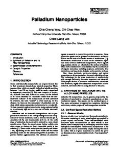
absorption optics). In contrast to the turbidity detector, these detector signals do not need any Mie correction. One example for a PSD obtained from a sedimentation run applying UV absorption optics is presented in the following [29]. As an example, very small platinum clusters with diameters of only 0.5 < dp < 2.0nm are chosen (see also our introduction sample on gold colloids in Fig. 1.2). This example (presented in Figs. 3.22 and 3.23) demonstrates also the capability of AUC to investigate even smallest nanoparticles. A platinum cluster system was synthesized by reduction of platinum tetrachloride in water with formic acid in the presence of the stabilizer alkaloid dihydrocin quinoline, as described in [30]. The colloid was dispersed in a mixture of acetic acid and methanol (5:1 by volume), using ultrasonic stirring for 5–10 min. The density of the solvent at 25 ◦ C was determined as ρs = 1.0182g/ml, and its viscosity as ηs = 0.01167 Poise. The density of the stabilized platinum particles ρp was found to be close to that of bulk platinum, ρPt,25 ◦ C = 21.5g/cm3 [31]. The concentration c0 was not known precisely, but it was so low that one worked within the linear range of the UV detector (λ = 380nm), which means A < 1.5 was always valid. From the different XL-A/I UV scans of Fig. 3.22 at different running times, it becomes clear that one must carefully select the radial scan that is used for the evaluation of the particle size distribution. In the early stages of the experiment, the complete fractionation of the different species in the mixture is not yet achieved, whereas in the late stage, bigger particles may already have reached the cell bottom,

Fig. 3.23. Integral and differential particle size distribution of the Pt colloid in Fig. 3.22. The thickly marked scan in Fig. 3.22 (at running time 18 min) was used for the PSD evaluation (reprinted with permission from [29])

86

3 Sedimentation Velocity

and would therefore not be detected. As a suitable radial scan, we chose a scan at 18min from the middle of the run, indicated in Fig. 3.22 by means of a thick line. The corresponding particle size distribution, both in integral and in differential form, is presented in Fig. 3.23. This multi-modal (!) particle size distribution is characterized by a distinct number of monodisperse species. The evaluation and comparison of the particle size distributions for further radial scans of Fig. 3.22, taken of the same Pt colloid at different running times t, yielded (within the errors of measurement) the same particle size distribution. This means that there is only a weak diffusion broadening of most of the components within this particle size distribution (or perhaps a selfsharpening of the different boundaries; see Sect. 3.3.2). Upon analysis of the same Pt colloid by electron microscopy (EM), a continuous, only bimodal (apparent) particle size distribution is detected, with average particle sizes of 1.0 and 2.2 nm for the two main components. Nevertheless, this rough agreement is a proof that the absolute AUC dp values in Fig. 3.23 are in the correct order. The striking feature in Fig. 3.23 is the presence of seven different, resolved monodisperse species that differ only by 0.1nm in their particle diameter. As such Pt clusters are very small, the broad peak around 0.83nm (component number 8) must be considered with some caution, because it does not reflect the true particle size distribution, due to the expected high diffusion effect for such small clusters.

3.6 Synthetic Boundary Experiments Synthetic boundary experiments in the AUC have been performed since the 1950s. They are a special form of sedimentation velocity experiments. Earlier work on this topic has been published by Kegeles [32] and Pickels [33]. The measuring cells applied in synthetic boundary cells have already been described in Sect. 2.3 and Fig. 2.7. Whereas most AUC laboratories use synthetic double-sector boundary cells of the capillary type (available for the XL-A/I), in the authors’ laboratory synthetic boundary cells of the valve type are applied predominantly: mono-sector valve-type cells (older Model E cells) are used for Schlieren optics (see Fig. 2.7e), whereas double-sector valve-type cells (homemade at BASF) are preferred for interference and UV optics. The essential part of each kind of synthetic boundary cell is the corresponding centerpiece. Since this versatile and useful double-sector valve-type centerpiece is at present not available from the manufacturer (Beckman-Coulter), our own homemade centerpiece is published as a sketch in Fig. 3.24. This sketch may be used by those interested to have produced a replica in a good mechanical workshop. Figure 3.24 shows a workshop drawing and a photograph. In principle, our centerpiece is only a modification of the mono-sector valve-type centerpiece shown in Fig. 2.7e, as used in the older Beckman Model E. Nevertheless, there are three differences between the BASF-made and the older Beckman valvetype centerpieces: (i) our centerpieces, in particular the double-sector centerpiece,

3.6 Synthetic Boundary Experiments

87

Fig. 3.24. Workshop drawing and photograph of a homemade (BASF) 12-mm double-sector valvetype titanium centerpiece for synthetic boundary runs, required for interference and UV optics. The photograph shows also the storage bin (reservoir) with the thin ventilation pipe, the filling hole screw, the cylinder-shaped rubber valve, and two gaskets

88

3 Sedimentation Velocity

the storage bin with its small ventilation pipe, and the tightening screw, are all made of titanium. It is therefore possible to use these for all kinds of solvents, also aggressive ones; (ii) the filling hole, and the tightening screw of the solvent sector are not on the meniscus side, as usual, but rather on the bottom side; and (iii) as rubber valve, we use a cylinder-shaped piece (diameter 1.2 mm), cut out from chemical-resistant Kalrez O-rings for organic solvents, and from Viton for aqueous systems. By varying the length of this rubber cylinder, it is possible to vary the rotor speed ωoverlay , at which overlaying starts. In the following, only experiments performed in cells of the valve type or equivalent cells are described. These valve-type cells (like the capillary-type cells) regulate the overlaying of a liquid from a reservoir (storage bin) onto the liquid column in the sector-shaped chamber of the measuring cell. This results in a sharp boundary between the two liquids, which is additionally stabilized by the centrifugal field. It has been shown that is advantageous if the liquid to be overlaid by the liquid from the reservoir exhibits a slightly higher density (in the magnitude of Δρ = 10−4 g/cm3 , [34]), in order to avoid turbulences. The sedimentation experiment itself is usually performed in an angular velocity range of 10 000 < ω < 40 000rpm, depending on the actual analytical problem. The design of the capillaries, as well as the rubber functioning as a valve, allow the user to vary the rotor speed ωoverlay at which overlaying occurs. Typical rotor speeds to start overlaying are in the range 5000–10 000rpm for the valve-type cells. The valve-type cell facilitates a more defined overlaying than the capillary-type cell, by varying the hardness (crosslinking) or the cylinder length of the rubber valve, especially for organic solvents with their low interfacial tensions (these interfacial tensions create serious problems with capillary-type cells). There are four main applications of synthetic boundary experiments, described in the following four subsections, these being (i) dynamical density gradients, (ii) determination of very small s values, (iii) determination of D values, and (iv) determination of loading concentrations c0 and (dn/dc)p . Dynamical Density Gradients Fast dynamical density gradients are the most prominent application in the authors’ laboratory. This is another kind of fast (completed within 10 min!) H2 O/D2 O analysis (see Sect. 3.5.3) to measure particle densities ρp , and their possible distribution. The dynamical density gradient is described in this subsection (rather than the density gradient; cf. Chap. 4) because it vividly illustrates how the valve-type cell works to create a synthetic boundary. Figure 3.25 shows that Schlieren optics and simple mono-sector valve-type cells have been used in most cases. Figure 2.7e shows a photograph of the centerpiece of such a cell, with the storage bin, rubber valve and ring-like gasket outside of the centerpiece. A gravity valve (a compressed rubber cylinder) under the small hole of a potlike storage bin (reservoir), filled with water (or other media), opens at a rotor speed of about 10 000rpm, and subsequently all light H2 O inside this storage bin will be overlaid onto the heavier D2 O inside the cell sector. Because of the

3.6 Synthetic Boundary Experiments

89

Fig. 3.25. Schematic illustration of a synthetic boundary experiment, using a 12-mm mono-sector valve-type cell/centerpiece (left). As an example, real Schlieren photographs of a dynamic H2 O/D2 O density gradient run of polystyrene latex particles, c = 0.4 g/l, are shown (right)

90

3 Sedimentation Velocity

H2 O/D2 O inter-diffusion (visible as a negative Gaussian Schlieren peak in Fig. 3.25), within these 10min a radial dynamic density gradient ρs (r), from ρs = 1.00 up to 1.10g/cm3 , is built up within the cell (visualized as a ρ axis in the lowest Schlieren photograph). Polystyrene latex particles (which show turbidity) dispersed in this D2 O (c0 = 0.4g/l, dp ≈ 100nm) gather within this 10-min period in a narrow turbidity band at that radius position where the densities of the particles ρp and the density gradient are identical. The experiment in Fig. 3.25 yields ρp = 1.055g/cm3 , the well-known value of polystyrene particles. For details of the evaluation to obtain these ρp values, see Sect. 4.3. For a standard synthetic boundary run with a valve-type cell (for example, to detect low molar mass solute in a solution or in a dispersion), H2 O in the storage bin is replaced by the pure solvent, and D2 O in the cell sector by the solution. Usually, the solute concentrations are in the range 0.3–10 g/l, but also much higher concentrations reaching 100g/l are possible (see Fig. 3.26). Determination of very Small s Values In many cases, only synthetic boundary runs allow us to determine s values of very small particles/molecules by creation of an artificial boundary over the air/liquid meniscus. This facilitates avoiding the problem that especially small particles or polymers tend to stick to the air/liquid meniscus due to interfacial tension. Thus, in many sedimentation velocity experiments performed on slowly sedimenting samples (mostly because of low molar mass), the meniscus is not cleared even at highest centrifugal rates. In such cases, the overlaying technique allows us to clear the meniscus, and to measure sedimentation coefficients as low as s = 0.2S (e.g., for saccharose having a molar mass of M = 300g/mol; [5, 34]). Conventional sedimentation velocity experiments usually have a lower limit of approximately 1S. Determination of D Values Determination of diffusion coefficients D of dissolved samples (M range 100 < M < 100 000g/mol) can be done by synthetic boundary runs. The overlaying of (slowly) sedimenting molecules/macromolecules in solutions (or in dispersions) with a pure solvent (or a dispersion medium) results in a steep, step-like radial change of the sample concentration c(r) within the cell around the radial position of the synthetic boundary roverlay (see Fig. 3.26). The steep step function, directly visible via interference optics (see Fig. 3.26a), broadens with increasing experimental time due to diffusion of the sample molecules into the pure solvent. Via Schlieren optics, a narrow (Gaussian) Schlieren peak is visible at this boundary (see Fig. 3.26b). Measurement of the broadening of the interference fringes or of the Schlieren peak as a function of running time t can directly be correlated to the diffusion coefficient D of the sample (see, for example, [35]). The results are of high accuracy if the sample is monodisperse. In fact, this type of measurement has been state of the art in diffusion coefficient determination until laser technology and dynamic light scattering (DLS) were introduced. Still today, this is a method that can be applied favorably for complex systems, or if only a very low amount of sample is available.

3.6 Synthetic Boundary Experiments

91

Fig. 3.26. a Radial XL-A/I interference optics scans, and b Schlieren optical photographs of two synthetic boundary experiments, taken at different experimental running times. In both cases, (turbid) latices (c0 = 100 g/l) with additional low molar mass solute (about 3 g/l) in the aqueous serum were measured. The diffusion broadening of the boundary due to the (non-sedimenting) low molar mass solute can be well recognized at the radial overlay position roverlay

92

3 Sedimentation Velocity

Determination of Loading Concentrations c0 and (dn/dc)p Synthetic boundary runs are also used to measure loading concentrations c0 and (dn/dc)p . At the radial overlaying position roverlay (see Fig. 3.26), the function of the refractive index over the radius in the cell n(r) shows a steep step due to the corresponding increase of the solute concentration c(r). This measurable change of refractive index Δn = (nsolution − nsolvent ) is detected either as a step ΔJ (interference optics, Fig. 3.26a) or as a peak area Aschl (Schlieren optics, Fig. 3.26b). The detected signal Δn can either be utilized for high-accuracy measurement of the solute concentration cp if the specific refractive index increment (dn/dc)p is known, or vice versa, the signal can be used to measure the specific refractive index increment if the loading concentration is known. For the case of interference optical detection of the synthetic boundary experiment (see (3.31)), a modification of (2.3) gives the correlation between the fringe displacement ΔJ, the light wavelength λ used, the specific refractive index increment (dn/dc)p , the length of the optical path through the cell a, and the concentration difference of the solute before and after the concentration step Δcp (usually Δcp = c0 ):

Δcp =

ΔJ · λ 

a·

dn dc



(3.31)

p

For the case of Schlieren optical detection (see Fig. 3.26b), the corresponding relation between Δcp and the Schlieren peak area Aschl is given as

Δcp =

Aschl · tan Θ   dn L · a · mx · my · E2 dc p

(3.32)

In (3.32), Θ is the Philpot angle of the Schlieren optics, E the magnification factor from cell to plate, L the enlargement factor due to the cylindrical lens, mx the path length of the solution in the cell, and my the distance from the center of the cell to the plane of the phase plate. Such synthetics boundary runs to determine cp (especially with interference optics) are also important for sedimentation equilibrium runs to measure M (see Sect. 5.2). They allow one to check whether the law of conservation of mass is fulfilled. Beside the above mentioned four main applications there are other applications of the synthetic boundary technique, such as the measurement of differential sedimentation coefficients [36], and the determination of extinction coefficients [37] should simply be noted here. Figure 3.26 shows two typical synthetic boundary experiments to detect small amounts of low molar mass solutes in the serum of aqueous particle dispersions, (i) with a double-sector valve-type cell, using the XL-A/I interference optics, and (ii) with a mono-sector valve-type cell, using the XL-SO Schlieren optics. In both examples, much higher total concentrations of c0 = 100g/l are chosen to detect, beside the major component of the (fast) turbid particles, with diameters of about

3.6 Synthetic Boundary Experiments

93

dp = 250 and 400nm, respectively, also any minor components of (slow) low molar mass solutes. In both cases, pure water was overlaid onto the aqueous polymer dispersions. In the interference optics scans of Fig. 3.26a, we see the large ΔJ step of the very fast, 250-nm particles only in the first two scans. Later, we see only the smaller step (ΔJ = 8.7), and the diffusion broadening of the slow (s = 0−0.2S) low molar mass solute (abbreviated “lmms”) at the overlay position roverlay . If we assume ( dn/dc)lmms = 0.15cm3 /g, a concentration of clmms = 3.3g/l follows with (3.31). This is about 3.3 wt% of the total solid content of the analyzed dispersion. In the four Schlieren optical photographs of Fig. 3.26b at different running times, the fast turbidity front of the 400-nm particles is visible only in the first Schlieren photograph (taken after 1min). Surprisingly, however, we see (for the first time in the second photograph, taken after 8min) a second, more slowly sedimenting, weak turbidity front (correlated with a small Schlieren peak). This was an unexpected 2-wt% component of small, 25-nm latex particles. Additionally, we found in all Schlieren photographs, permanently at the roverlay position, the small Schlieren peak of the low molar mass solute (s = 0−0.2S). From its Schlieren peak area Aschl,lmms follows, with (3.32), a concentration of clmms = 3.0g/l. This corresponds to about 3wt% of the total solids content of this dispersion. The diffusion broadening of this low molar mass solute Schlieren peak is clearly seen, too. In the following Sect. 3.6.1, we would like to present one unusual application of a synthetic boundary experiment, namely, synthetic boundary crystallization. Despite the fact that this experiment is not of common use and pronounced interest, it should inspire creativity and show that new types of AUC experiments are still conceivable. 3.6.1 Synthetic Boundary Crystallization Ultracentrifugation The basic idea of this method is to make use of synthetic boundary cells to perform chemical surface reactions inside the AUC while the centrifugal field acts. From the field of biological systems, two interesting approaches of (chemical) reactions within a synthetic boundary cell should be mentioned:

Fig. 3.27. Schematic representation of the synthetic boundary crystallization process inside the cell of an analytical ultracentrifuge

94

3 Sedimentation Velocity

(i) the active enzyme centrifugation, where the chemical reaction between an enzyme and its substrate is investigated [38], and (ii) the investigation of the formation of a polyelectrolyte membrane [39]. The synthetic boundary crystallization method was developed to investigate the early stages of crystallization. So far, it has been applied only to a system of low solubility, such as cadmium sulfide [40]. In this example, a 10mM sodium sulfide solution was overlaid onto a 5 mM cadmium chloride solution, which additionally contained 0.5 mM stabilizing thiols. At the sharp (synthetic) boundary between the two solutions, the nucleation of the hardly soluble cadmium sulfide particles takes place (see scheme in Fig. 3.27). For detection, the XL-A/I UV scanner (λ = 370nm) was used. The experiments were performed in 12-mm synthetic boundary doublesector cells of the Vinograd type, which is a capillary type with a small reservoir for the liquid used for overlaying (similar to the mono-sector capillary-type cell in Fig. 2.7d). Upon their formation, the very small CdS particles either continue to grow in the boundary region, or sediment toward the bottom of the cell into the cadmium chloride solution. This movement quenches any further growth, and allows us therefore to investigate the particles formed early in the process, as well as their particle size distribution.

Fig. 3.28. Comparison of (apparent) particle size distributions obtained from synthetic boundary crystallization experiments from three differently stabilized CdS nanoparticle systems via XL-A/I UV scans at λ = 370 nm (reprinted with permission from [40])

3.6 Synthetic Boundary Experiments

95

The efficiency of the stabilizers in such experiments has been successfully studied by Börger and Cölfen [41]. The particle sizes obtained in these experiments are in the magnitude of 1–3 nm (see Fig. 3.28), using ρp = 3.2g/cm3 for the density of the CdS particles. Figure 3.28 shows also that, of the three investigated stabilizers, thioglycerine is the most effective because it yields the smallest CdS particles, having an (average) diameter of only 0.9 nm.

References 1. Stafford WF (1992) In: Harding SE, Rowe AJ, Horton JC (eds) Analytical ultracentrifugation in biochemistry and polymer science. The Royal Society of Chemistry, Cambridge, p. 358 2. Kehrhahn JH, Lechner MD, Mächtle W (1993) Polymer 34:2447 3. Stafford WF (1994) In: Schuster TM, Laue TM (eds) Modern analytical ultracentrifugation. Birkhäuser, Berlin, p. 119 4. Fujita H (1975) Foundations of ultracentrifugal analysis. Wiley, London 5. Schachman HK (1959) Ultracentrifugation in biochemistry. Academic Press, New York 6. Gofman JW, Lindgren FT, Elliott H (1949) J Biol Chem 179:973 7. Mächtle W (1984) Colloid Polym Sci 262:270 8. Börger L, Kühnle A (2003) Unpublished data 9. Creeth JM, Knight CG (1965) Biochim Biophys Acta 102:549 10. Johnston JP, Ogston AG (1946) Trans Faraday Soc 42:789 11. Schachman HK (1951) J Am Chem Soc 73:4453 12. Gilbert GA (1960) Nature 186:882 13. Bowen TJ, Rowe AJ (1970) An introduction to ultracentrifugation. Wiley, London, p. 107 14. Lechner MD, Mächtle W (1995) Prog Colloid Polym Sci 99:120 15. Lechner MD, Mächtle W (1999) Prog Colloid Polym Sci 113:37 16. van Holde KE, Weischet WO (1978) Biopolymers 17:1387 17. Yphantis DA (1984) Biophys J 45:324 18. Schuck P (2000) Biophys J 78:1606 19. Schuck P, Rossmanith P (2000) Biopolymers 54:328 20. Schuck P, Perugini MA, Gonzales NR, Howlett GJ, Schubert D (2002) Biophys J 82:1096 21. Mie G (1908) Ann Phys 25:377 22. Mächtle W (1988) Angew Makromol Chem 162:35 23. Heller W (1957) J Phys Chem 26:498 24. Scholtan W, Lange H (1972) Kolloid Z Z Polym 250:782 25. Mächtle W (1999) Biophys J 76:1080 26. Mächtle W (1984) Makromol Chem 185:1025 27. Mächtle W (1992) Makromol Chem Macromol Symp 61:131 28. Müller HG, Herrmann F (1995) Prog Colloid Polym Sci 99:114 29. Cölfen H, Pauck T (1997) Colloid Polym Sci 275:175 30. Bönnemann H, Braun GA (1996) Angew Chem Int Ed 35:1992 31. Lide DR (ed) (2002) CRC Handbook of chemistry and physics, 83rd edn. CRC Press, Boca Raton 32. Kegeles G (1952) J Am Chem Soc 74:5532 33. Pickels EG (1952) Methods Med Res 5:107 34. Schachman HK, Harrington WF (1954) J Polym Sci 12:379 35. Aminabhavi TM, Munk P (1979) Macromolecules 12:1194 36. Hersh R, Schachman HK (1955) J Am Chem Soc 77:5228 37. Voelker P (1995) Prog Colloid Polym Sci 99:162 38. Kemper DL, Everse J (1973) In: Hirs CHW, Timasheff SN (eds) Active Enzyme Centrifugation and Methods in Enzymology, vol XXVII. Enzyme structure, part D. Academic Press, New York, p. 67 39. Wandrey C, Bartowiak A (2001) Colloid Surf A Physico Chem Eng Asp 180:141 40. Börger L, Cölfen H, Antonietti M (2000) Colloids Surf A 163:29

96

41. 42. 43. 44. 45.

3 Sedimentation Velocity

Börger L, Cölfen H (1999) Prog Colloid Polym Sci 113:23 Cölfen H (2004) ACS Symp Series 881:119 Harding SE (1995) Carbohydrate Polym 28:227 Oth J, Desreux V (1954) Bull Chim Belges 63:133 Schilling K (1999) PhD Thesis, Potsdam University, Potsdam

4 Density Gradients

The two major types of basic AUC experiments are the sedimentation velocity experiment (subject of Chap. 3), and the sedimentation equilibrium experiment (subject of Chap. 5). The density gradient experiment, topic of this Chap. 4, can be understood as a special kind of the sedimentation equilibrium experiment. Figure 4.1 illustrates the transition from Chap. 3 to Chap. 4, which means from the time-dependent sedimentation velocity runs to the time-independent static (equilibrium) density gradient runs. In Fig. 4.1a, this transition is experimentally done for dissolved macromolecules by simply adding 25 wt% of a heavy co-solvent, such as di-iodomethane (with a density of ρDIM = 3.2g/cm3 ), to the light solvent of the s run, tetrahydrofuran (with a density of ρTHF = 0.8811g/cm3 at 25 ◦ C). The density gradient experiment then takes considerable time, about 17 h in this example, until a radial exponential density gradient ρ(r) is built up within the cell. The density range covered in this case reaches from 1.0 to 1.2 g/cm3 . The gradient is built up due to enrichment of the heavy co-solvent near the cell bottom. Simultaneously within this 17h, the polystyrene molecules (M = 1 800 000g/mol, c = 1g/l) sediment (positive Schlieren peak in Fig. 4.1a) or float (negative Schlieren peak in Fig. 4.1a) to that radius position where the densities of the gradient and the particles/macromolecules are identical. This radial position is called the isopycnic position riso . The higher the molar mass M of the sample examined, the narrower becomes the detected final (constant) double Schlieren peak. The reason is diffusion broadening around this isopycnic position. In Fig. 4.1b, this transition from sedimentation run to equilibrium run is done for dispersed nanoparticles by simply adding 11wt% of a heavy iodinated sugar, metrizamide (ρ = 2.155g/cm3 at 25 ◦ C), to the (light) water. Again, within 16h a radial exponential density gradient, 1.03 < ρ(r) < 1.10g/cm3 , is built up within the cell, and the starting broad turbidity band of the dispersed polystyrene particles (dp = 160nm, c = 1g/l) is compressed to a narrow turbidity band at a radius position riso with ρ = 1.053g/cm3 , the known density value of polystyrene particles. The evaluation of density gradients such as the one in Fig. 4.1, the calculation of the shape and broadness of the double Schlieren peak and of the relation ρ(r), as well as the introduction of other types of density gradients (such as dynamic density gradients) is the topic of this Chap. 4.

98

4 Density Gradients

Fig. 4.1. a Sedimentation velocity experiment (s run) in THF and organic static 75 THF/25 DIM density gradient experiment (DG run) of narrowly distributed dissolved polystyrene molecules (Mw = 1 800 000 g/mol). b s run in H2 O and aqueous static 89 H2 O/11 metrizamide DG run of polystyrene latex particles (dp = 160 nm). For all runs: N = 40 000 rpm, 12-mm mono-sector cells, c = 1 g/l, Schlieren optics, Philpot angle = 70° (reprinted with permission from [19])

The chapter is structured as follows: Sect. 4.1 explains the basic principle of density gradients. In Sect. 4.2, the static (or sedimentation equilibrium) density gradient, the most frequently applied type of density gradient experiments, will be described, including the theory, data evaluation, experimental procedure, gradient materials, and examples. Section 4.3 deals with the fast dynamic density gradient, not commonly used by the AUC community, but of outstanding importance in the AUC laboratory at BASF. The experimental details as well as details of data evaluation are given. In Sect. 4.4 one exotic dynamic, but mandatory type of density gradient experiment, the aqueous dynamic Percoll density gradient, is presented.

4.1 Introduction In density gradient centrifugation experiments, a radial density gradient ρ(r) is induced in the measuring cell either by a heavy auxiliary additive added to a light solvent or by a mixture of two solvents exhibiting very different densities (see Figs. 4.1 and 4.2). The binary mixture has to consist of agents of different densities that are separated or accumulated differently within the measuring cell. The component with the higher density accumulates more in direction of the cell bottom. The relative composition of the solvent is different at each radial position r of the measuring cell. Thus, the density of the binary mixture varies throughout

4.1 Introduction

99

Fig. 4.2. Schematic presentation of a static AUC density gradient. The chemical composition, and therefore the density ρs (r) of the binary solvent DG mixtures varies with the radius r in the measuring cell. Depending on its density in comparison to the surrounding solvent density, the sample sediments or floats. At one radial position in the cell, the solvent density matches the sample’s density ρp . The sample accumulates at this position

the cell, exhibiting higher densities at the bottom of the cell and lower densities at the meniscus. In the following section, we will refer to the binary mixture as solvent, meaning that we will use the parameter ρs (r) = ρDG (r), having in mind that this is arguable. The sedimentation behavior of a sample (containing macromolecules or nanoparticles) added to such a (binary) density gradient is determined partly by the buoyant term (1 − υ · ρs ), according to (1.5), or by the density difference between particle density and density of the density gradient (ρp − ρs ), according to (1.9), where ρp = 1 / υ. If the sample component occupies a radial position in the density gradient exhibiting a solvent density that is lower than its own density, then the particle or polymer will sediment toward the cell bottom. In the opposite case, the component will float toward the meniscus. If particle/macromolecule density ρp and solvent density ρs are equal, no movement will occur (see Figs. 4.1 and 4.2). The sample component has then reached its isopycnic position riso within the cell. Together with the choice of an appropriate gradient material and proper experimental conditions, the main challenge in isopycnic centrifugation is to build up the relation between the radial position r and the (binary) density gradient mixture density, i.e., ρs (r). Several approaches for this (see [3]) are established. Some of these will be described in Sects. 4.2.1 and 4.3. Appropriate optical detectors locate the radial position riso of the sample (Schlieren optics is most important, as in

100

4 Density Gradients

Fig. 4.1, but also all other detectors are possible, if the density gradient medium is transparent). Cheng and Schachman were the first to perform a kind of density gradient experiment in 1955 [1], where they made use of the high compressibility of fluorotoluene. The high compression at high rotor speed induces a radial density gradient throughout the AUC cell. In a double-sector cell, two droplets were added to this fluorotoluene system: first, one droplet of an aqueous buffer solution, and second, a droplet of the same buffer solution containing additionally a dissolved polymer (having a slightly increased density). As water and the organic solvent are not miscible, the droplets as a whole moved within the gradient to a radial position where their known densities were matched. This allowed an accurate evaluation of the relative density difference between the buffer solution and polymer-containing buffer solution, as well as the determination of the absolute density values. These droplets of known density are called density markers. The first equilibrium density gradient experiments that were performed in the manner sketched above [2] were already subject of discussion in the introduction to this book (Chap. 1, Figs. 1.4 and 1.5). The impact of the H2 O/CsCl density gradient experiment of Meselson and Stahl on double-stranded DNA in scientific history is beyond controversy. Also nowadays, however, density gradients are of great help in analyzing manifold (macromolecular/nanoparticulate) systems. Thus, it is not astonishing that isopycnic centrifugation is well established in biochemical research, with H2 O/CsCl as the standard density gradient. Again, to the authors’ surprise, the use of density gradient methods in the field of synthetic polymers and colloids is not common, despite the fact that density gradient experiments are excellent tools for the characterization of dispersed nanoparticles in the diameter range 10nm–10 μm (see examples in Chap. 6). Also, dissolved synthetic macromolecules can be well subjected to density gradients, taking advantage of the high fractionation resolution of analytical ultracentrifuges. As the densities of particles and macromolecules depend on their chemical composition, the AUC density gradient experiments are beneficial for highly sophisticated analysis of complex polymeric or colloidal systems. Due to this ability, density gradients have also been called “density spectroscopy” [3]. This “density spectroscopy” is visualized in Fig. 4.3 (see also Figs. 4.5 and 4.12). The upper part of Fig. 4.3 shows schematically the particle densities of the most frequently used aqueous homopolymer dispersions (latices) arranged as turbidity bands in a density gradient along a ρ axis according to their particle densities ρp . Via copolymerization (and reactions on the surfaces of all kinds of particles), thousands of other particles with nearly all densities between them can be created. AUC density gradients allow one to measure these particle densities (and their distribution, too!) very precisely, and with an extremely high resolution of Δρp = 0.0003g/cm3 (in special cases). Thus, such reactions can be analyzed via density gradients, and the expression “density spectroscopy” is indeed justified. Chapter 6 presents real application examples. The lower part of Fig. 4.3 shows the accessible density ranges of some differently composed water/metrizamide density gradients.

4.2 Static Density Gradients

101

Fig. 4.3. Particle densities of the most common homopolymer latices, arranged along a density ρ axis (upper part), and accessible density ranges of nine differently composed static water/metrizamide AUC density gradients (lower part). This figure illustrates what is called “AUC density spectroscopy” (reprinted with permission from [3])

Preferential solvation of one of the two density gradient components does not play any role in the analysis of bigger (compact) nanoparticles, i.e., if dp > 30nm is valid. For this reason, absolute particle densities can be measured with an accuracy of Δρp = ±0.002g/cm3 . For very small particles, however, and especially for dissolved macromolecules, preferential solvation can play a role and falsify the measured density values. Thus, for example, in Fig. 4.1a, because of preferential solvation of the light THF, the polystyrene density value of the dissolved macromolecules is shifted slightly to an apparently lower value ρ = 1.04g/cm3 , if one compares this with the “true” value ρ = 1.055g/cm3 of compact polystyrene particles in Fig. 4.1b. Nevertheless, also in the presence of preferential solvation, density gradients are a valuable analytical tool because of their high fractionation power according to chemical composition. Again, this is demonstrated in Chap. 6.

4.2 Static Density Gradients Static equilibrium density gradients are the most frequently used density gradient experiments. In the authors’ industrial R&D laboratory, they are tools of daily use as they allow easy and unambiguous analysis of known and unknown complex colloidal and/or polymeric systems.

102

4 Density Gradients

4.2.1 Theory of Static Density Gradients The theoretical description of density gradients has to cover the following aspects: (i) Formation and evaluation of the radial static density gradient ρs (r). (ii) Radial distribution of the examined sample within the density gradient. From the literature, several approaches for the determination of particle and/or polymer densities from experimental data obtained in static equilibrium density gradient experiments are known (see [3]). The aim of all of these approaches is to build up a solvent density over radius function ρs (r). Once this relation is known, only the radial (isopycnic) positions riso of the sample’s fractions have to be known to determine their densities. There are two ways to obtain ρs (r): (i) via theoretical calculation, and (ii) via calibration with different markers of known particle density ρp . Both ways are described in the next two sections. Formation and Calculation of the Radial Static Density Gradient ρs (r) The correct treatment of the formation of the density gradient ρs (r) can be carried out similarly to that of sedimentation equilibrium experiments (see Chap. 5) applying thermodynamic laws, but with the difference that in the case of density gradients the (heavy) equilibrium-forming component is usually present in a very high concentration. Therefore, activities ac , rather than concentrations c, have to be considered (this is the weak point of all density gradient theories!). For the following derivation, we continue to use concentrations, rather than activities, bearing this restriction in mind. The gradient has formed when equilibrium between sedimentation and diffusion of the binary mixture, forming the density gradient, is reached. Therefore, the net mass flow at each radial position dm/dt within the cell is zero. Starting from (1.13), the mass transport equation, this leads to (4.1):  ∂c ∂c dm 2 = φ ar csω r − D = 0 ⇒ csω2 r = D . (4.1) dt ∂r ∂r In (4.1), the parameters s, D and c, as well as the parameters υ and M in the following part of this section, refer to the heavy component (for example, CsCl, di-iodomethane (DIM), metrizamide, or Nycodenz) of the binary density gradient mixture. Besides this, (4.2) holds:

∂c ∂c ∂ρs = · ∂r ∂ρs ∂r

(4.2)

Replacing the quotient s/D of the sedimentation coefficient s and the diffusion coefficient D in (4.1) by the expression from the Svedberg equation (1.8), and inserting (4.2), the following (4.3) is obtained:  M ω2 r ∂ρs ∂ρs  = 1 − υ · ρs ∂r ∂ ln c RT

(4.3)

4.2 Static Density Gradients

103

This can be rearranged to give (4.4):

∂ρs ω2 r = ∂r β(ρs )

(4.4)

where β(ρs ) is given by (4.5):

β(ρs ) =

∂ ln c RT ∂ρs (1 − υ · ρs )M

(4.5)

As the concentration c of the heavy gradient component determines the solvent density, the function β(ρs ) varies only with the density ρs . In flat density gradients (i.e., at low c and low rotor speed ω), which exhibit no intense variation of the solvent density, β(ρs ) can be assumed to be constant over radius. Thus, an empirically evaluated value can replace it (for aqueous CsCl gradients, the value was found to vary between ca. 1.13 × 109 and 1.21 × 109 cm5 g−1 s−2 ; [4]). The density at any given radial point in the cell can then be calculated by (4.6), which is obtained by integration of (4.4) under the assumption that β is constant:

ρs (r) = ρs,0 +

1 2 ω (r − r0 )2 2β

(4.6)

For the calculation, a reference point at a radial position r0 with known density ρs,0 has to be given. This problem is often overcome by addition of marker particles with known densities to the density gradient. The detection of the radial position of these makers delivers r0 , and allows us to calculate the density at any other radial position within the measuring cell. Ifft et al. [5] calculated β values for five aqueous gradient-forming substances (CsCl, KBr, RbBr, RbCl, and sucrose) from listed values for density and activity over the full density gradient range covered by the materials (roughly 1.0–2.0g/cm3 ). The resulting plots of β(ρs ) versus density were then fitted by polynomial functions such as (4.7):

β(ρs ) = β0 + β1 · ρs + β2 · ρs2 + β3 · ρs3 + ... + βk · ρsk

(4.7)

The determined constants, βi , are listed for the five systems in [5], leading to reliable results when used in the evaluation of the five aqueous density gradient systems mentioned above. In the same paper, the concept of the isoconcentration point is introduced. The basic idea is as follows: if a measuring cell, filled with a density gradient solution of concentration ci of the heavy gradient-forming compound, is centrifuged until equilibrium is reached, a position ri in the gradient must exist that exhibits exactly the initial concentration ci of the solution, and thus the initial (constant) average density ρs,i (see Fig. 4.4). This point is called the isoconcentration point, ri . Again taking β as being constant, (4.6) becomes (4.8) in this special case:

ρs (r) = ρs,i +

1 2 ω (r − ri )2 2β

(4.8)

104

4 Density Gradients

The advantage of this isoconcentration approach is that ri can be calculated via geometrical considerations (see Fig. 4.4). As approximation to ri , the arithmetical mean between rm , the radius of meniscus and rb , the radius of bottom, was proposed. A better approach for sector-shaped cells is the geometrical mean given in (4.9) [5]:  2 + r2 rm b ri = (4.9) 2 It has to be kept in mind that this ρs (r) evaluation does not take into account pressure effects (see Sect. 3.3.3), and therefore it is applicable only in restricted cases, or not applicable at all in (often strongly compressible) organic density gradients. Still, it works well in aqueous systems. Hermans and Ende first addressed organic density gradients in 1963 [6]. These authors introduced a new approach for the evaluation of density gradients: the so-called Hermans–Ende theory. This theory describes density gradients under the assumption that the organic binary density gradient system behaves like an ideal mixture. The derivation of this theory will be described in the following. Given is an ideal binary mixture of two components (light/heavy) with indices 0 and 1, and volume fraction ϕ0 of components 0 and volume fraction ϕ1 of component 1, defined by (4.10): n Vk0 nk Vk0

ϕk =  k k

m vk0 mk vk0

=k

k = 0, 1 ,

(4.10)

k

Fig. 4.4. Definition of the isoconcentration point in a static density gradient. At the beginning of the experiment, a uniform concentration ci of the gradient-forming material is given in the whole measuring cell. After the equilibrium is reached, one point in the cell at radial position ri exhibits the initial concentration, and therefore the initial known solvent density ρs,i

4.2 Static Density Gradients

105

with the molar amount of substance nk , the mass mk , the molar volume Vk0 , and the specific volume vk0 of the component k. Equation (4.10) leads to (4.11) in the case of binary density gradient mixtures:

ϕ0 + ϕ1 = 1

(4.11)

According to Hermans and Ende [6], the ratio of the volume fractions as a function of the radius is given by (4.12), a kind of barometrical equilibrium equation:

ϕ0 2 = α · e β·r ϕ1 Equation (4.13) gives the expression for the integration constant sector-shaped cells:    2 exp β · ϕ1in · rb2 − rm −1     α= 2 in 2 2 exp β · rb − exp β · ϕ1 rb + β · ϕ0in rm

(4.12)

α in (4.12) for

with the initial volume fraction of component k, ϕkin . The constant (4.14):    M1  2 ω · ρ1 − ρ0 ρ1 β= , 2RT

(4.13)

β is given by

(4.14)

with the molar mass of the heavy component 1, M1 , and the densities of the components 0 and 1, ρ0 and ρ1 . The density of an ideal solution is given by (4.15):

ρs = ϕ0 · ρ0 + ϕ1 · ρ1

(4.15)

The combination of (4.11), (4.12) and (4.15) results in the so-called Hermans–Ende equation, (4.16):   ρ0 + ρ1 · α · exp β · r2   ρs (r) = (4.16) 1 + α · exp β · r2 This Hermans–Ende equation is applicable for all kinds of static equilibrium density gradients, for organic ones and for aqueous ones. Under the assumption that α · exp(β · r2 ) 20nm), and not for slowly sedimenting dissolved macromolecules (discussed in the following section). The marker calibration technique ([3]; Figs. 4.5–4.7) can also be regarded as a kind of “dynamic” density gradient method (during the time to reach equilibrium), because no equilibrium is really needed to measure absolute sample particle densities in this way. Distribution of the Sample Within the Static Density Gradient Whereas in the above section the formation of the density gradient and the evaluation of the resulting solution densities ρs (r) were described, the distribution of sample material to be analyzed within the gradient will be the subject of the following section. In this section, an equation will be derived showing that, at the stage of equilibrium, (monodisperse) sample particles are distributed around their radial equilibrium position r0 in the density gradient following a Gaussian-like curve (see Figs. 4.9 and 4.10a). The radial derivation of such a Gaussian Schlieren curve is a double Schlieren peak, such as those shown in Figs. 4.1a and 4.8. The equilibrium condition for the pure gradient solution given in (4.1) is assumed to be valid also in the presence of small amounts of dissolved macromolecules and dispersed particles. This is fulfilled because csample 30nm. Dissolved macromolecules are not analyzable with dynamic density gradients because they do not move fast enough. The density range of dynamic H2 O/D2 O density gradient experiments can be shifted [15] to either side by adding a third component to the H2 O/D2 O mixture (as for static density gradients, see Sect. 4.2.2 and Fig. 4.3). Most commonly used as shift agents are methanol (ρmethanol = 0.793g/cm3 at 25 ◦ C) to extend the range to lower values, and ethylene glycol or glycerin (ρethylene glycol = 1.114g/cm3 and ρglycerin = 1.261g/cm3 ) for shifting to higher values. From this third component, significant additional complications arise, as mixing enthalpies, etc., have to be taken into account. Thus, the overall conclusion is that dynamic H2 O/D2 O density gradients are suited for the density range 0.85 < ρs (r) < 1.25g/cm3 . To demonstrate the fractionating power of the dynamic density gradient performed in the AUC, we give one example here (another example was presented in Fig. 3.25 above). The same mixture of 11 polymeric latex particles (see Table 4.1) used to set up the marker calibration evaluation of static equilibrium density gradients (see Sect. 4.2.1 and Fig. 4.5) is investigated in a dynamic H2 O/D2 O density gradient experiment. According to Table 4.1, five components of the mixture are expected to exhibit densities in the range covered by this dynamic density gradient between 1.0 and 1.1 g/cm3 . Figure 4.12 shows four Schlieren optical pictures of the corresponding experiment, taken at 0.5-, 4-, 6- and 10-min experimental running time at the standard rotor speed 40 000rpm. The Schlieren photograph taken after 0.5min (in the startup phase of the rotor at about 5000rpm) shows the measuring cell before overlaying has occurred. The cell is half filled with D2 O, which contains the dispersed (turbid) sample (ctotal = 3g/l, i.e., about 0.19g/l of each component). In the next Schlieren picture (taken after 4min), the meniscus moves to the top of the cell during the overlaying of H2 O onto the D2 O phase, because the valve opens at about 10 000 rpm. The dynamic density gradient has already formed at the H2 O/D2 O interface. In the course of the experiment, the components of the sample having densities below 1.0g/cm3 or above 1.1g/cm3 will float or sediment out of the region of the gradient. The expected five components are fractionated within the region of the density gradient, and form narrow turbidity bands. The particle densities determined, using (4.29), the 10min photograph and the procedure described in Fig. 4.11, are 1.004, 1.021, 1.043, 1.067 and 1.089g/cm3 . These values correspond very well

124

4 Density Gradients

Fig. 4.12. Four Schlieren optical pictures of a dynamic H2 O/D2 O density gradient experiment performed on a mixture composed of 11 polymeric latex components with different particle densities. The pictures are taken after 0.5, 4, 6, and 10 min. Five of the 11 density fractions are recorded within this density gradient range. A 12-mm mono-sector valve-type synthetic boundary cell was applied. The ρs (r)-axis below the 10 min photograph was calculated as described in Fig. 4.11 (reprinted with permission from [18])

with the independently measured “true” values (Kratky balance) 1.000, 1.021, 1.043, 1.066 and 1.089g/cm3 , given in Table 4.1. This experiment is an impressive demonstration of (i) the fractionating power, and (ii) the high (absolute!) precision of the dynamic density gradient as well as (iii) the short duration of the analysis: Within only 10min, much information on sample composition is gained. Again,

4.4 Other Types of Density Gradients

125

Fig. 4.12 is a good example for what we call “density spectroscopy” via AUC density gradients. It is interesting to note that this experiment in Fig. 4.12, done in an analytical ultracentrifuge, was repeated in a preparative ultracentrifuge, using 38-ml tubes (see Sect. 7.2 and Fig. 7.5).

4.4 Other Types of Density Gradients Beside the two main types of density gradients (the static equilibrium, and the dynamic density gradients) described in this Chap. 4, there are other types of density gradients. Examples are the preparative dynamic density gradient (see Sect. 7.2), density gradient-related techniques such as the pH gradient (see Sect. 7.2), and the dynamic Percoll density gradient (see Sect. 4.4.1). These have in common that they are not (yet) applied broadly, and thus are not so much of practical interest. Nevertheless, as new approaches are also envisaged, it is worth considering at least the principles of alternative types of (density) gradient experiments. One example of such an exotic density gradient, the aqueous Percoll density gradient, will be discussed in more detail in the following section. 4.4.1 Percoll Density Gradient A special type of fast dynamic AUC density gradient experiment, the (analytical) dynamic Percoll density gradient, was introduced by one of the authors in 1984 [16]. It allows one to analyze particle densities in the range 0.85–1.15 g/cm3 within the timescale of a sedimentation velocity experiment, i.e., within 30min. For this dynamic Percoll density gradient, simple standard cells, mono- or double-sector cells, are used, rather than synthetic boundary cells such as those used in the dynamic H2 O/D2 O density gradient described above in Sect. 4.3. The principle of this type of experiment is described in the following. Figure 4.13 shows a TEM micrograph and the particle size distribution of Percoll. This is a dispersion of very small Percoll nanoparticles in water, supplied by Pharmacia Fine Chemicals, Uppsala, Sweden. Percoll consists of inert SiO2 particles coated with polyvinyl pyrrolidone (PVP). The density of the Percoll particles is ρPercoll = 1.992g/cm3 (at 25 ◦ C), particle sizes varying in the range 5–35 nm (see Fig. 4.13). The original aqueous Percoll dispersion, as supplied by Pharmacia, has a particle concentration of cPercoll = 24wt%, and a total density of ρ = 1.135g/cm3 . This aqueous Percoll dispersion, diluted to 12 wt% with water, is subjected to a sedimentation velocity run (see Fig. 4.14). Usually, the standard conditions are: 20 000rpm, 3-mm mono-sector cells, and Schlieren optics. Three Schlieren pictures, after 20-, 30- and 40-min running time, are shown in Fig. 4.14. They yield an average sedimentation velocity coefficient s = 180S for these Percoll particles (but there is a considerable s distribution of 40 < s < 600S). Because of the relatively broad particle size distribution of the Percoll particles, the Schlieren peak representing the sedimentation boundary of these Percoll particles is broadened with increasing experimental time, as the boundary moves

126

4 Density Gradients Fig. 4.13. Transmission electron microscopy (TEM) picture and particle size distribution of Percoll particles. Artificial black spots representing 100- and 800-nm particles are added to the TEM micrograph in order to illustrate the size ratios between the density gradient-forming Percoll particles and the analyzed polystyrene latex sample (reprinted with permission from [16])

toward the bottom of the AUC measuring cell. Within this sedimentation boundary, i.e., within the radial range of the corresponding Schlieren peak, the Percoll concentration c(r) changes from zero at the upper end of the sedimentation boundary (near the meniscus) to 12wt% at the lower end of the boundary (near the bottom) where the boundary passes into the plateau region with constant Percoll concentration. The radial concentration change c(r) is associated with a radial density change ρs (r) varying from 1.0g/cm3 in the pure solvent region (= pure water) to the density of the starting, 12-wt% Percoll dispersion, 1.06g/cm3 in the region of constant Percoll concentration. Therefore, the integration of the Schlieren optical signal in Fig. 4.14 (at a defined running time) yields directly the radial density gradient course ρs (r) (in analogy to the dynamic H2 O/D2 O density gradient, (4.29) and (4.30) in Fig. 4.11). In the upper 20-min Schlieren photograph of Fig. 4.14, the result of this integration is visualized as a ρ axis (parallel to the r axis). This ρ axis varies with the running time t, i.e., it shifts increasingly in the direction of the cell bottom. It can be summarized that by performing a standard sedimentation

4.4 Other Types of Density Gradients

127 Fig. 4.14. Schlieren optical pictures of a sedimentation velocity run of a dispersion of 12-wt% Percoll particles dispersed in H2 O. Pictures taken after 20, 30, and 40 min. Due to the different sedimentation velocities of the differently sized PVPcoated SiO2 particles (5 < dp < 35 nm), the Schlieren peak is broadened in the course of the experiment. This creates a radial dynamic density gradient ρs (r, t) in the region of the Percoll peak (1.00 < ρs (r) < 1.06 g/cm3 ), shown as a ρ axis below the 20-min photograph (reprinted with permission from [16])

128

4 Density Gradients Fig. 4.15. Schlieren optical pictures of a dynamic 88 H2 O/12 Percoll density gradient experiment of a polystyrene latex sample consisting of 800-nm particles (cPS = 0.01 g/l). The turbidity band caused by the rapidly sedimenting/floating polystyrene particles stays at its relative position of equal density throughout the experiment, and sediments together with the Percoll Schlieren peak toward the cell bottom (reprinted with permission from [16])

4.4 Other Types of Density Gradients

129

velocity run with Percoll particles, a relatively fast dynamic density gradient ρs (r, t) is established within 20–40 min in an AUC. This can be advantageous, as will be shown in the following. In Fig. 4.15, Schlieren optical pictures of another experiment performed similarly to that described above are shown. In this case, a small amount of an aqueous polystyrene dispersion (cPS = 0.01g/l, consisting of big latex particles 800nm in diameter) is added to the Percoll dispersion. In addition to the broadened Schlieren peak of Percoll, a narrow turbidity band can now be observed. This turbidity band is formed by the polystyrene particles, which move very fast, within minutes, by simultaneous sedimentation and flotation, to their isopycnic radial position riso in this dynamic Percoll density gradient. The turbidity band remains in the region of the Percoll peak, and does not show further relative sedimentation or flotation, compared to the Percoll peak. Together with the Percoll Schlieren peak, the turbidity band sediments completely to the cell bottom. The radial position of the turbidity band within the Percoll density gradient can easily be analyzed at any given running time, and thus ρp calculated. From all photographs in Fig. 4.15, the obtained density of the turbidity band is the same, i.e., ρp = 1.052g/cm3 . This value corresponds very well with the known density of polystyrene latex particles (ρPS = 1.055g/cm3 ), a fact that can be taken as a proof of concept. The relatively limited density range of dynamic water/Percoll density gradients can be shifted to 0.85–1.15 g/cm3 by substitution of the H2 O by either methanol (for lower densities) or heavy water D2 O (for higher densities). For details of experiments performed on samples containing different density fractions, unknown samples, and even on living biological cells, the reader is referred to [16]. The dynamic aqueous Percoll density gradient is restricted to large particles (dp > 100nm), which sediment much faster than the Percoll particles.

References 1. 2. 3. 4. 5. 6. 7. 8. 9. 10. 11. 12. 13. 14. 15. 16. 17.

Cheng PY, Schachman HK (1955) J Am Chem Soc 77:1498 Meselson M, Stahl FW, Vinograd J (1957) Proc Natl Acad Sci 43:581 Mächtle W, Lechner MD (2002) Prog Colloid Polym Sci 119:1 Thomas CA, Berns KI (1961) J Mol Biol 3:277 Ifft JB, Voet DH, Vinograd J (1961) J Phys Chem 65:1138 Hermans JJ, Ende HA (1963) J Polym Sci Part C Polym Symp 1:161 Fujita H (1962) Mathematical theory of sedimentation analysis. Academic Press, New York Van Holde KE, Baldwin RL (1958) J Phys Chem 62:734 Rolfe R (1962) J Mol Biol 4:22 Rockwood D (ed) (1984) Centrifugation, a practical approach, 2nd edn. IRL Press, Oxford Correia JJ, Weiss GH, Yphantis DA (1977) Biophysical J 20:153 See http://rasmb-email.bbri.org/rasmb_search.html Hexner PE, Radford LE, Beams JW (1961) Proc Natl Acad Sci 47:1848 Rossmanith P, Mächtle W (1997) Prog Colloid Polym Sci 107:159 Lange H (1980) Colloid Polym Sci 258:1077 Mächtle W (1984) Colloid Polym Sci 262:270 Dale D, Gladstone F (1858) Philos Trans 148:887

130

4 Density Gradients

18. Mächtle W (1999) Prog Colloid Polym Sci 113:1 19. Mächtle W (1992) In: Harding SE, Rowe AJ, Horton JC (eds) Analytical ultracentrifugation in biochemistry and polymer science. The Royal Society of Chemistry, Cambridge, p. 147 20. Mächtle W, Klodwig U (1979) Makromol Chem 180:2507 21. Lechner MD, Mächtle W, Sedlack U (1997) Prog Colloid Polym Sci 107:148 22. Lechner MD, Borchard W (1999) Eur Polym J 35:371

5 Sedimentation Equilibrium

5.1 Introduction Sedimentation equilibrium runs in an AUC – in short, “equilibrium runs” – are long-duration runs of 10–200 h. The essential is that during this long time, equilibrium is reached between sedimentation to the cell bottom and (back-) diffusion of the dissolved (macro) molecules inside the solution column. This means that the radial concentration distribution c(r) of the solute inside the measuring cell is independent of time or, in other words, the left-hand term in Lamm’s equation ((1.10) or (1.15)) is zero, which means that dc/dt = 0 is valid all times. There are two kinds of equilibrium runs in an AUC – first, the static density gradient run to measure densities ρp of dissolved macromolecules and particles, and second, the sedimentation equilibrium run to measure molar masses M of dissolved macromolecules. In the case of polydisperse solutes, the sedimentation equilibrium run allows us to measure the different average molar masses, Mn , Mw , Mz (see also Sect. 3.4.2 and (3.18)), and the complete molar mass distribution W(M), where  ci  Mn = is the number average molar mass, (5.1a) ci · Mi−1  ci Mi is the weight average molar mass, (5.1b) Mw =  ci  ci Mi2 Mz =  is the z-average molar mass (5.1c) ci · Mi and ci is the mass percentage of the component i with molar mass Mi within the whole polydisperse polymer. Density gradient runs are already broadly treated in Chap. 4, and thus this Chap. 5 deals only with the sedimentation equilibrium run to measure molar masses M and molar mass distributions W(M). In addition to the sedimentation equilibrium method, there are some other AUC methods to measure M (see Sect. 5.5), but the sedimentation equilibrium method is the most important one. Beside the AUC, there are other methods to measure molar masses and molar mass distributions, such as the scattering methods (static light scattering (SLS), small angle neutron scattering (SANS), small angle X-ray scattering (SAXS)), osmometry, viscosimetry, size exclusion chromatography (SEC), gel electrophoresis,

132

5 Sedimentation Equilibrium

and matrix-assisted laser desorption/ionization time-of-flight mass spectrometry (MALDI-TOF-MS). However, the AUC is one of the most powerful and versatile tools, especially to determine molar mass distributions (see example in Sect. 3.4.2), because a fractionation according to Mi takes place within the AUC measuring cell. In contrast to SEC and gel electrophoresis, which are relative methods, the AUC is an absolute method, which means that no calibration standards are necessary to measure molar masses. Additionally, the AUC covers the broadest range of molar masses, from about 300 up to several million Dalton (g/mol). This is possible because the rotor speed ω can be varied easily between 500 (for high M) and 60 000rpm (for small M). The basic equation of sedimentation equilibrium runs used to calculate M from the measured concentration distribution c(r) (for monodisperse solutes in an ideal non-interacting solution, where A2 = 0 is valid, and at infinite dilution c → 0) follows from Lamm’s equation (1.15) for dc/dt = 0, or more simply, from the net mass transport equation (1.13) for dm/dt = 0 to   dc/dr s = 2 (5.2) D ω rc and further, by substituting s/D by means of the Svedberg equation (1.8), to M

RT (dc/dr)  · rc 1 − ν · ρ ω2

=

(5.3)

or, with dc/c = d ln c and 2r dr = d(r2 ), to M

d ln c 2RT  · 2 dr2 1−ν·ρ ω

=

(5.4)

This final basic equation (5.4) says that a plot of the logarithm of concentration c(r) versus the square of the radial distance r2 should give a straight line (see, for example, Fig. 5.3b), with the slope being directly related to the molar mass M of the (monodisperse!) solute. In the case of a polydisperse solute in a non-ideal solution (A2 > 0), this straight line will be transformed into a curvilinear line (upwardbending in the case of polydispersity/association, and downward-bending in the case of non-ideality). A careful analysis of this curvature will yield the molar mass distribution of the solute, as well as information on possible interactions, such as self-association, or on the thermodynamic quality of the analyzed solution, i.e., about the association constants Ka or the second virial coefficients A2 . This analysis is the main topic of Chap. 5. The sedimentation equilibrium method was used extensively in the years 1950– 1970 for molar mass measurements of biopolymers, especially for proteins. Nowadays for proteins, amino acid sequencing and gel electrophoresis is much faster and more precise. Nevertheless, still today only the equilibrium method allows us to study reversible associations of proteins in solution (see Sect. 5.4.2). In the years

5.2 Experimental Procedure

133

1950–1980, molar mass determinations via the equilibrium method, using the old analytical ultracentrifuge of Beckman, the famous “Model E”, was a tedious, long procedure, because of working with photo-plates, special calibrations, a complex digitization of the photo-plates in a comparator by hand, and manual graphical extrapolations. Nowadays, all these problems are eliminated with the new Beckman Optima XL-A/I machine, which is fully computerized and digitized via a CCD camera and an image processing system, delivering 100-fold more measuring data than before, and having an eight-cell rotor multiplexer. For synthetic polymers and especially synthetic polyelectrolytes, which are mostly broadly distributed, molar mass determinations via the equilibrium method have now become easier, faster, and more precise. We will demonstrate that in this Chap. 5 by presenting only measurements on synthetic polymers (with one exception in Sect. 5.4.3). There are many publications about the sedimentation equilibrium method in the literature. For a deeper study and for further details, we recommend the following review articles: Creeth and Pain [1], van Holde and Baldwin [2], Chervenka [3], Yphantis [4], and Harding et al. [5].

5.2 Experimental Procedure Equilibrium runs in an AUC to measure molar masses M can be done with all optical systems: Schlieren optics, interference optics, or the UV/VIS scanner. The latter is appropriate only if the solute shows absorption, and if the solvent is transparent for the corresponding wavelength λ. This is always valid for aqueous solvents (i.e., for biopolymers and polyelectrolytes), but it is not valid for the most common solvents of synthetic polymers, such as toluene, THF and DMF. These solvents show strong UV absorption, so that the dissolved polymer is “invisible”. Thus, interference optics is the universal detector, and mostly used for synthetic polymers. Figure 5.1 shows the primary results (before data evaluation) of a standard equilibrium run recorded with the three different optical systems mostly used: a UV scan (done with an Optima XL-A/I), and a combined interference and Schlieren photograph (both done with an old Model E during the same run). In the new Optima XL-A/I, these “photos” are done with a digital CCD camera (see the interference “photos” made by an Optima XL-A/I in Fig. 5.2). All three scans/photographs in Fig. 5.1 show the typical result of an equilibrium run: an exponential radial course of the concentration distribution c(r) within the measuring cell. The standard measuring cell is a double-sector cell with a thickness of a = 12mm, and with the corresponding window holder (UV, interference or Schlieren). Also 3- or 25-mm centerpieces (aluminum, Epon or titanium, the latter is recommended for organic and aggressive solvents) are possible. The initial concentration c0 of the solute should be as low as possible to be near the ideal state c → 0. On the other hand, c0 depends on the sensitivity of the optical system chosen: 0.05–1.00 g/l for the most sensitive UV scanner, 0.5–10.0g/l for the interference optics, and 2–40 g/l for the Schlieren optics. For non-ideal solutions, a series of concentrations c1 , c2 , c3 , ... is recommended (three for the four-cell rotor,

134

5 Sedimentation Equilibrium Fig. 5.1a,b. Typical primary results of standard equilibrium runs to measure molar masses. a A radial UV scan, and b a combined Schlieren and interference photograph, using 12-mm double-sector cells, 2.5-mm filling heights, and an artificial FC-43 oil bottom (reprinted from [3] and [6] with permission)

and seven for the eight-cell rotor). This allows us to carry out the necessary extrapolation c → 0. Sapphire windows are here preferred for optical reasons, compared to quartz windows in the case of interference optics. The total measuring time tequil needed to reach equilibrium is proportional to the square of the cell filling height, (rb − rm )2 , according to [2]. Thus, measuring times of hours up to weeks are possible. In practice, one chooses a 2–3 mm length of the solution column (as in Fig. 5.1), in order to be close to the equilibrium state within about 24h. Also short column equilibrium runs with filling heights of 0.5– 1.0mm and shorter running times of only 3–10h are possible. Although these M determinations by short column runs are not very precise, especially in the case of polydisperse samples, they may be used for analyzing (mostly monodisperse) proteins. In contrast to former days, with the tedious, manual comparator evaluation of photo-plates, it is today much easier to check whether the equilibrium state is really reached. This is done by continuous automatic scans during the whole equilibrium run, until comparisons between following scans do not show any difference within the detector sensitivity. Only the last scan and its digital data are used for the evaluation of the molar mass M and the molar mass distribution W(M). Because the measuring data at both ends of the solution column are very important, it is common practice to use a small artificial bottom (about 0.5mm in

5.2 Experimental Procedure

135

Fig. 5.2. Example of a typical standard sedimentation equilibrium run with seven different concentrations of the NBS 706 polystyrene in toluene. The upper part shows the seven primarily taken interference “photos” of an Optima XL-A/I, and the lower part the resulting (classical) evaluation, delivering Mw and A2

136

5 Sedimentation Equilibrium

height) of heavy FC-43 oil (3M Company) to better visualize the bottom area. Thus, not only the upper meniscus rm of the column is clearly visible and measurable, but the lower meniscus at the bottom, rb , too. The heavy FC-43 oil is not miscible with most common solvents, so that it forms a transparent cushion under the solution column during the run. As a result, the standard filling procedure of a standard 12-mm double-sector cell for an equilibrium run (see Fig. 5.1) is the following: to start with, fill the solution compartment with 0.03 ml FC-43 oil, and add 0.12ml of solution. Then, fill the solvent compartment with 0.17ml solvent (essentially, the dialyzate of the sample solution has to be used in the case of biopolymers and polyelectrolytes). This results in a standard length of the solution column of about rb − rm = 2.5mm. The absolute temperature T during an equilibrium run is not so important but not so its constancy, because temperature gradients within the cell give rise to remixing of the radial exponential equilibrium concentration profile c(r), which leads to falsifying this profile. Usually T is 20 or 25 ◦ C. The choice of the optimal rotor speed ω depends on the molar mass M of the analyzed sample. It is reasonable to start with 10 000rpm, and adjust during the run to the optimal speed. This optimal speed is reached if at the equilibrium state the relation of sample concentration at the bottom cb to the concentration at the meniscus cm is between 3:1 and 10:1. A modern way to find the optimal ω and an estimation of tequil are the simulation routines using the program “Ultrascan” ([33]), and a rough estimation of the expected M value. A special case, where cm = 0 is valid, we call meniscus depletion run (for details and the evaluation procedure, see Yphantis [4]), but this method is not very precise. It especially fails for broadly distributed polymers (to prove cm = 0, one needs longer solution columns, rb − rm ). In order to reach the equilibrium state faster, often overspeeding is used, which means choosing for the initial 3h of an equilibrium run a rotor speed that is 1.5 times higher than the final speed. The basic equilibrium run equations (5.3) and (5.4) at the beginning of this Chap. 5 show that for the calculation of M, beside T, ω and the measured concentration  profiles, c(r) or dc/dr(r), a precise knowledge of the important buoyancy term 1 − ν · ρ is needed. Often the partial specific volume ν of the solute, and the solution density ρ (which is approximately the density of the pure solvent) are known from the literature or tables. If not, we have to measure it (as described in Sect. 2.6.1) with a high-precision Kratky density balance on a concentration series (5, 10, 20g/l) of the solute in the solvent used. To transfer the primary measured radial profiles of the absorption A(r), the refractive index n(r), or refractive index gradient dn/dr(r) (see Fig. 5.1) into the secondary concentration profile c(r) used for calculating M, specific optical solute/solvent constants are needed. For the absorption optics, this is the specific decadic absorption coefficient ε, and for the interference and Schlieren optics this is the specific refractive index increment dn/dc (usually, as described in Sect. 2.6.2, dn/dc is measured by means of a high-sensitivity or a differential refractometer, using the same concentration series as that used for the ν determination).

5.2 Experimental Procedure

137

For the absorption optics, this transfer relationship (see [6]) between the absorbance A = lg(I0 /I) and the concentration c is given by Lambert-Beer’s law (2.2), A(r) = lg(I0 /I(r)) = εc(r)a, if ε is known from the literature or tables. If ε is not known, any equilibrium run can deliver ε with the help of the law of conservation of mass,

1 c(X) dX

= c0

(5.5)

0 2 2 where c0 is the initial concentration, and X = (r2 − rm )/(rb2 − rm ) is the normalized squared radius r. Combination of (2.2) and (5.5) gives the wanted

ε=

1 c0 a

1 (5.6)

A(X) dX 0

As c0 , a and ∫ A(X) dX are obtained experimentally, ε may be easily determined from equilibrium runs with absorption optics. The parameter ε depends considerably on the selected UV wavelength λ. A presupposition for the validity of this procedure is that the total amount of solute is recorded within the A(X) signal, and no (high molar mass) parts of the solute have completely sedimented to the cell bottom. For the interference optics (and the Schlieren optics – not presented here), this transfer relationship can be derived in a similar way. Because the vertical shift of the interference fringes J is proportional to the concentration c (see Sect. 2.4.2 and (2.3)), in analogy to the absorption optics and the Lambert-Beer equation (2.2), the following relation is valid: 



ΔJ(X) + Jm λ c(X) = a(dn/dc)

(5.7)

where ΔJ(X) = (J(X) − Jm ) is the number of fringes shifted in relation to the meniscus position of the chosen fringe at the (radial) distance X, and Jm is the unknown (absolute) number of fringes at the meniscus. Again, Jm can be calculated with the help of the equation for the conservation of mass, (5.5), via the following relation: Jm

= J0 −

1 0

ΔJ(X) dX =

c0 a(dn/dc)

λ

1 −

ΔJ(X) dX

(5.8)

0

where J0 = (c0 a( dn/dc))/λ, calculated with (2.3), is the total number of fringes of the initial concentration c0 . Again, as c0 , a, dn/dc, λ, and ∫ ΔJ(X) dX are obtained experimentally, Jm and also c(X) may be determined from equilibrium runs with interference optics. If c0 of the initial concentration is not known, it is possible to

138

5 Sedimentation Equilibrium

determine J0 with a synthetic boundary run of that solution (see Sect. 3.6). The accuracy of AUC M measurements via interference optics depends essentially on the accuracy of the Jm determination (see also [20]). For nearly all measuring methods of molar masses M, also for the equilibrium run, we need to know the initial concentration c0 of the starting solution. An M value is always only as precise as this value c0 . Usually, c0 is determined in a relatively precise manner by weighing in the solid solute into the solvent. However, there are cases where this is not possible, for example, if there is a ready solution with an unknown concentration c0 . In this case, one can solve the problem by a synthetic boundary run of this solution within the AUC, and determine c0 as described in Sect. 3.6. We would like to conclude the description of the experimental procedure with a typical example of a standard equilibrium run, shown in Fig. 5.2: the primary interference “photos”, taken first by means of an Optima XL-A/I CCD camera within the same run, where seven different concentrations of a polystyrene sample, dissolved in toluene, were measured simultaneously. Also shown are the resulting molar mass Mw and the second virial coefficient A2 , delivered by a complex evaluation. How this data analysis is handled will be described in the following Sect. 5.3.

5.3 Data Analysis This Sect. 5.3 is divided into four parts. In Sect. 5.3.1, we present the well-known classical evaluation of sedimentation equilibrium runs, and the corresponding equations to calculate M of monodisperse samples, and Mw and Mz of polydisperse samples. In Sect. 5.3.2, we describe a powerful nonlinear regression evaluation method, created by Lechner in 1991, to determine the complete molar mass distribution W(M), using (i) a versatile three-parameter model molar mass distribution W(M, P, B, K), and (ii) also the Mw and Mz values of the classical evaluation, in Sect. 5.3.1, as starting parameters for the nonlinear regression. Lechner’s method is particularly well suited for polydisperse samples. Section 5.3.3 shows practical applications of the classical and of the nonlinear regression evaluation methods. In Sect. 5.3.4, we outline the M-STAR evaluation method (M ∗ ), which delivers, as does the classical evaluation, an Mw value without the need of a model. The M-STAR program can be used as a pre-evaluation program preceding any model-dependent evaluation. 5.3.1 Basic Equations for Molar Mass Averages – Classical Evaluation of AUC Equilibrium Runs The full theoretical thermodynamic foundation of the sedimentation equilibrium is given in the famous books of Fujita [7, 8]. The basic equation for the radial con2 2 )/(rb2 −rm ) at the sedimentation equilibrium centration c(r), or c(X) with X = (r2 −rm state can be described for non-ideal solutions (A2 , A3 , ... > 0) of monodisperse polymers by the following relation [8]:

5.3 Data Analysis

139

  1 − v2 ρ1 ω2 RT

r dr

=



1 se 2 d(ln c) + 2Ase 2 c + 3A3 c + ... M

 (5.9)

se where Ase 2 , A3 , ... are the virial coefficients of sedimentation equilibrium. This se (5.9) is essentially identical with the basic (5.3) and (5.4) for Ase 2 = A3 = ... = 0. For non-ideal solutions of polydisperse polymers, the following relation holds for the ith (monodisperse) component within that polydisperse sample with in all i = 1, 2, ..., q components [8]:

  1 − v2 ρ1 ω2 r dr RT

=

  q  d ln ci +2 A2ik dck + ... Mi

(5.10)

k=1

 Summation over all solute components i, and division by ci ≡ c(r) at distance r yields the “point” weight-average molar mass Mw (r) (see (5.1b) at a radial displacement r (or X): 2  2   2 2 rb − rm rb − rm ci Mi d(ln c) (dc/dr) d ln c  (5.11) = Mw,app (r) = = = 2 Λ d(r ) 2Λ c·r Λ dX ci with the constant

Λ=

    2 1 − ν2 ρ1 ω2 rb2 − rm 2RT

(5.12)

The suffix “app” in Mw,app (r) includes correction terms for non-ideality (i.e., for A2 , A3 > 0). The correct Mw (r) is obtained by extrapolating the Mw,app (r) values to zero concentration c → 0. As Schlieren optics measures dn/dr (which is proportional to dc/dr), rather than c(r), one has to rearrange (5.10) with respect to dn/dr ∼ dc/dr. This gives the “point” z-average molar mass Mz (r) (see (5.1c) at a radial displacement r (or X): 2      2 rb − rm 1 dc ci Mi2 d 2 d[ln(dc/dX 2 )]  ln = Mz,app (r) = = (5.13) 2 ci Mi Λ dr r dr Λ dX The operational “point” average molar masses Mw,app (r) and Mz,app (r) are functions of the radial distance r (or X) at a point in the ultracentrifuge cell or, in other words, the local molar masses defined by the local slopes of the c(r) curve or the dc(r)/dr curve. To obtain the real, r-independent average molar masses Mw,app and Mz,app of the whole polydisperse polymer, one has to carry out an integration of (5.11) and (5.13), from the meniscus to the bottom of the cell (with the use of the relation for the conservation of mass, (5.5)). The results of that integration are the two following, well-known equations:

140

5 Sedimentation Equilibrium

Mw,app

=

Mz,app

=

  cb − cm Λ · c0 2       2 rb − rm 1 1 dc 1 dc   − 2Λ cb − cm rb dr b rm dr m

(5.14) (5.15)

Equation (5.14) is called the Lansing–Kraemer equation [9], and (5.15) the Richards–Schachman equation [10], after the scientists who first derived these in 1935 and 1959. According to (5.14), we need only the difference cb − cm to calculate Mw,app , because all other values in this equation are known. This difference in concentration between the bottom of the cell and the meniscus can easily be determined directly by the UV scanner, using (2.2), or with interference optics by the (relative) number of shifted fringes at the cell bottom, ΔJ(rb ) = (Jb − Jm ), using (2.3):   cb − cm = Δc rb =

rm dc

=

rb

rm  rb

dc dr



dr =

    A rb − A rm aε

=

  Jb − Jm Λ (5.16) a(dn/dc)

For Schlieren optics, integration is necessary (not presented here). To calculate Mz,app according to (5.15) is more complex, because we need, in addition to cb − cm , the local slopes dc/dr at the radial positions rb and rm . These slopes are condc 2·Λ·c·r nected according to (5.11), as =  2 2  · Mw,app (r), with the two point dr rb − rm weight-average molar masses Mw,app (rb ) and Mw,app (rm ) at these radial positions. Introduction of these two relations into (5.15) yields Mz,app

=

    cb Mw,app rb − cm Mw,app rm   cb − cm

(5.17)

Equation (5.17) is identical with (5.15), and is also called the Richards–Schachman equation. In contrast to the calculation of Mw,app (see (5.14)), where we need only the difference of the concentration at the bottom and at the meniscus, cb − cm ), we now need for the calculation of Mz,app (see (5.17)) the absolute values of cb and cm , too. These values are delivered according to the procedure described in Sect. 5.2, using (2.2), (5.5) and (5.6) for absorption optics, as well as (2.3), (5.7) and (5.8) for interference optics. As has been pointed out above, all Mapp values include correction terms for nonideality. Correct molar masses M are obtained by an extrapolation Mapp → M. This is an extrapolation to infinite dilution c → 0. The exact necessary mathematical extrapolation relation is, according to [8], 1 Mapp

=

c + c   2 1 b m se cb + cm + 2Ase + 3A + ... 2 3 M 2 2

(5.18)

5.3 Data Analysis

141

However, if c is relatively low, a good approximation is 1 Mapp

=

1 se 2 + 2Ase 2 c0 + 3A3 c0 + ... M

(5.19)

In the following, we use only (5.19). The (classical) determination of number-average Mn (see (5.1a)) or (z + 1)average Mz+1 molar masses will in principle be possible with equations that are similar to (5.14) or (5.15). Nevertheless, the applicability is very restricted, due to larger experimental errors on determining intercepts, slopes and further derivatives of the primary experimental curves, i.e., of A(r), ΔJ(r), and dn(r)/dr ∼ dc(r)/dr, especially at the bottom of the cell and at the meniscus. It will be pointed out in the following Sect. 5.3.2 that the direct transformation (nonlinear regression) or the indirect (inverse Laplace) transformation of the reduced concentration profile Uw (X) = c(X)/c0 or the reduced concentration gradient profile Vw (X) = (dc(X)/dX)/c0 is more suitable for the determination of the molar mass averages Mn , Mw and Mz via an approximated three-parameter model W(M) than is the case with the classical evaluation method. If the determined approximated W(M) is of high quality, it allows us to calculate all needed average molar masses with (5.1), or with the integral form of this equation (see (3.18)). 5.3.2 Basic Equations for Molar Mass Distributions – Nonlinear Regression Evaluation (Lechner Method) The determination of the molar mass distribution W(M) of a polydisperse polymer via AUC equilibrium runs requires the connection of the experimentally measured, reduced concentration profile c(X)/c0 = Uw (X) (for absorption and interference optics), or the reduced concentration gradient profile ( dc(X)/dX)/c0 = Vw (X) (for Schlieren optics) with (i) the molar mass distribution function W(M), and (ii) the reduced concentration profile U(X, M) or the reduced concentration gradient profile V(X, M) of a monodisperse sample [8, 11–13]: Uw (X) =



c(X) c0

 c0 →0

=

∞ W(M)U(X, M) dM

e ΛMX U(X, M) = ΛM ΛM 0<X 20nm. Some Other New AUC Methods A drawback of static density gradients (see Chap. 4) are the long measuring times of 1–5 days necessary to reach equilibrium. However, during this process, every static density gradient is in principle also a dynamic one, ρ(r, t), i.e., it changes with time: the change is fast at the beginning of the experiment, and becomes progressively slower at the end. Basically, there are two possibilities to use these faster “pseudo-static” density gradients for analytical purposes. The first one is to calculate ρ(r, t) theoretically, as described above for the PDDG, but this can only be done when a new theory describing the attainment of static density gradient equilibrium will have been developed. The second option is to measure ρ(r, t) as a function of time: (i) by recording continuously the concentration c(r, t) of one of the two main density gradient components, which has already been realized by using metrizamide (or Nycodenz) in static H2 O/metrizamide density gradients (see [17]), or (ii) by adding sets of calibrated density markers to the density gradient (as for the 11-component latex particle mixture mentioned above), also recently realized in [18] (also see Sect. 4.2.1). As mentioned in Sect. 7.1 on the topic of “measuring cells”, new synthetic boundary cells offer the possibility of new analytical methods in the fields of studying surface reactions inside the AUC cell, e.g., the formation of polyelectrolyte

228

7 Recent Developments and Future Outlook

complexes and thin membranes, or studies of the first steps in crystal growth and metal cluster formation (see also [2] and [17] in Chap. 6). Above, we discussed different radial gradients within an AUC cell, in particular density, concentration, pH, and solubility gradients. However, we did not discuss the radial pressure gradient. Such a radial pressure gradient (see Sect. 3.3.3) is established within every AUC cell in every kind of AUC run, also in a pure solvent. It is independent of time, and the function p(r) can be calculated if rotor speed, filling height, solvent density, and solvent compressibility coefficient κ are known. At maximum rotor speed (60 000rpm), the radial pressure gradient varies from 1bar at the meniscus to 250bar at the bottom. It is conceivable to use this pressure gradient for some analytical purposes. For example, one could measure compressibility coefficients κ of solvents and solutions, or of single macroscopic particles introduced into such pressure gradients. It should also be possible to study the compression of gels as a function of pressure (see [29] and [30]). In 95% of all AUC experiments performed worldwide, the sedimentation velocity method or the sedimentation equilibrium method are used, where fractionation is achieved according to size/molar mass. Only in 5% of the cases is the density gradient method used, mainly because of its high potential to fractionate according to particle density – in other words, according to chemical composition. Even today, the density gradient method is a nearly unknown continent in the AUC world. We recommend that the scientific community should explore it more intensively in the near future. The AUC particle sizing method, using a turbidity detector (see Sect. 3.5.1), is the most powerful and most perfect AUC method at present, especially in combination with the H2 O/D2 O analysis method (see Sect. 3.5.3). Nevertheless, it can still be improved. One improvement was proposed by us already [12], namely, the introduction of a second, parallel measuring laser beam into the PSD device (see Fig. 3.13). We also presented [12] initial successful measurements with a device having the first laser beam in the first third, and the second laser beam in the last third of the cell sector length (rb − rm ). However, the full potential of this new twobeam PSD method (or three, or even more beams!) has not been explored until now. We are confident that this modification will lead to improvements in PSD data quality and, in particular, allow us to carry out more precise H2 O/D2 O analyses. If the precision of measurement is high enough, then it will be possible to obtain the complete particle density distribution (in addition to the PSD), i.e., the chemical heterogeneity of an unknown latex sample. A higher precision could also lead to a higher density range of the H2 O/D2 O analysis, perhaps up to about 0.5–20g/cm3 , which is substantially wider than the range accessible by static density gradients (0.85–1.9 g/cm3 ).

7.3 New AUC Data Analysis High-precision multi-detection and powerful, fast online data analysis are the keys for a more frequent use of the AUC in the future, in particular for the investigation

7.3 New AUC Data Analysis

229

of complex inhomogeneous mixtures showing distributions in size, molar mass, density/chemical composition, electrical charge, shape, degree of crosslinking, etc. The aim is a global AUC analysis (perhaps in combination with other methods), and the simultaneous determination of all these different distributions. There is interdependence between multi-detection and data analysis, but at present data analysis is more developed as multi-detection. Nevertheless, also the data analysis should be improved. In the following, we will discuss three ways to improve the existing, and to develop new data analyses: (i) online controlling of the AUC instrument, (ii) improvement of measuring data quality via data analysis, and (iii) improvement of data evaluation of data analysis. Online Controlling of the AUC Instrument The registration of measuring data during AUC runs is not always really online (as in the case of turbidity, interference, and UV/Vis detectors). For example, data registration by Schlieren optics (mostly used for density gradients and some fast synthetic boundary runs) is still done via photographs on photo-plates, or by means of digital CCD cameras. When the AUC run is finished, these “photos” are evaluated offline. At present, no sophisticated PC programs are available to do this offline photograph evaluation fully automatically. Usually, manual help with a cursor on a PC TV screen is required, for example, to define rm and rb , or to follow the Schlieren curve. So far, there exists only one attempt in the literature [19] to replace this manual help by an automatic image-processing program. Thus, for the future of Schlieren optics, it is desirable to combine CCD photograph registration and image processing to obtain a real online data registration during the AUC run. Furthermore, it is desirable to have this automatic detection (and also controlling!) of rm and rb within the existing XL-A/I online data registration programs of the interference and the UV/Vis detector. Internally, the Optima XL-A/I is equipped with a computer that controls the machine and all relevant parameters, i.e., rotor speed, temperature, flash light, laser diodes, detectors, repetition rates of the scanning devices, etc. For safety reasons, this internal computer is not accessible for the operator of the XL-A/I, or only in a very restricted manner. However, it would be advantageous to have an additional external computer for the control of the XL-A/I by the operator in special cases. One option was already mentioned above, namely, selecting and controlling different rotor speed profiles ω(t). Another idea is to check the meniscus position rm continuously via continuous radial scans, and to detect in this way, for instance, any slow disturbing leakage of the cell. Continuous scans (together with continuous data analysis) can also be used to check reaching the equilibrium state in equilibrium and density gradient runs, and to stop the run automatically when there is no difference anymore (within the errors of measurement) between the last two successive scans, or when a 99% equilibrium is reached. In this way, it should also be possible to check the solvent plateau and the solution plateau continuously during sedimentation velocity runs, in order to make sure that the law of conservation of mass and the radial dilution rule (3.5) are fulfilled at all times. We hope somebody will develop such intelligent data analysis programs

230

7 Recent Developments and Future Outlook

in the near future to improve the control of the machine itself, and of the whole AUC run. Improvement of Measuring Data Quality via Data Analysis The best way to obtain high-quality measurement data is to use very sensitive detectors, with a signal-to-noise ratio as high as possible. However, physics determines the limits here. Also the data of the best detector can be improved by data analysis. A striking example is the time derivative method to evaluate sedimentation velocity runs (see Sect. 3.3.6 and [9]), a data analysis in which a significant improvement of the signal-to-noise ratio of the experimental data is reached by subtracting successive scans from each other, resulting in the elimination of systematic errors in the optical patterns, and a decrease of random noise. Imperfections and distortions of sapphire windows are a major problem for interference optics detection. They create time-independent distortion of the detector signal. Often these distortions increase with rotor speed. We propose to develop a data analysis that eliminates these distortions in the following manner. One uses always the same cells with the same windows, placed always in the same position within the cells, measuring these cells, filled only with solvent, at the usual standard rotor speeds and storing the resulting “blind” signal data in the evaluation computer. If real samples are measured, these stored blind signals are subtracted from the sample signal. Another possible way to eliminate window distortions is to record at the beginning of every run, immediately after the final rotor speed is reached, a first scan and to subtract this from all following measuring scans. The blank correction routine of the XL-A/I, and the two programs SEDFIT [7] and dc/dt [9] solve parts of this window problem for constant rotor speed, but not for the variable rotor speed technique ω(t). One way to reduce statistical noise is to use as many scans as possible, followed by averaging. This is valid for each kind of evaluation. This is a need especially for the present XL-A/I UV/Vis detector. To realize this, we need, as mentioned above, a radial scanning device much faster than the existing one. This would allow us to multiply the number of scans per run. Another disturbing problem is the presence of UV-active impurities in solvents and samples. It is conceivable to eliminate this problem by improving the measuring signal, as proposed above, via “blind” scans, or scans at the beginning or at the end of a run, which are subtracted subsequently from the measuring scans. Scans at the end of the run are preferred, but only if the sample has sedimented completely to the cell bottom. Beside a faster scanning device, new data analysis programs that subtract this impurity noise, if possible automatically and online, are required to carry out such corrections. There are first programs [28] that are indeed able to do this, but they should be improved and work really online. Schlieren optics data can be improved in two ways via data analysis. The first, also by additional “blind” photographs, is to correct for (i) inhomogeneous illumination of the cells, and (ii) pixel heterogeneities, and possible dark currents of the CCD camera (see [19]). The second way is by developing a powerful image processing program to analyze such corrected CCD Schlieren photographs (see,

7.3 New AUC Data Analysis

231

for example, Figs. 3.24, 4.1, 4.7, and 4.13), involving (i) the radial calibration and automatic detection of radial positions of the meniscus, bottom and turbidity bands in density gradients, (ii) determining the coordinates of Schlieren curves and the areas of Schlieren peaks, and (iii) extracting from a series of Schlieren photographs, taken during a sedimentation velocity run, the complete distribution of the sedimentation coefficient g(s) = dG(s)/ds. Indeed, A. Rowe and coworkers, University Nottingham, England, are developing a Schlieren online evaluation. The extraction/construction of g(s) “master curves”, as mentioned in Sect. 7.1, is important for very broadly distributed samples, and is a difficult task for all optical detection systems. Unfortunately, the time derivative method [9] fails for such broadly distributed samples, where all components of the sample can not be seen simultaneously on single or two successive scans/photographs. In the first scans of such a sedimentation velocity run, we see only the fast, large components, and in the last scans we see only the slow, small components. However, if it would be possible to combine all these different time-dependent scans into a single timeindependent g(s) “master curve” by means of a new data analysis program, then this would be the key to a renaissance of molar mass distribution measurements via AUC. As mentioned above, there are first attempts to realize this [26, 27]. Improvement of Data Evaluation Once we have the best possible primary measuring data, these data have to be transformed subsequently via evaluation programs into sedimentation and diffusion coefficients, sizes, molar masses, particle densities, or into the corresponding distributions. For this transformation, we need physical theories and a good data evaluation/analysis. At present, there are physical theories for most of the evaluation problems, but some of these should be improved. One missing theory is, as mentioned above, the time dependence of cs (r, t) during sedimentation equilibrium and static density gradient runs to reach final equilibrium. There is also a need for a theory to calculate more precisely the radial density function, ρ(r), within static density gradients (see Chap. 4 and [20–22]). Good evaluation theories are already existing, too. Nevertheless, improvements and new developments are desirable. A first step to make the fast Archibald runs (see Sect. 5.5) attractive again for molar mass measurements is the recent evaluation program of Schuck and Millar [23]. For calibration of static density gradients with marker particles of known densities [18], one needs better interpolation programs to calculate ρ(r) for every rotor speed, filling height, and mixing ratio of the two gradient components. Some evaluation programs do not offer possibilities to correct for effects of, for example, pressure, concentration and speed dependence, or Johnston–Ogston and non-ideality (see Sects. 3.2 and 3.3). However, these correction possibilities should be part of every program. Also, the correction of diffusion broadening during sedimentation velocity runs of very broadly distributed samples should be improved. A global AUC data analysis of the future could be a combination of all single data analysis programs: Archibald, time derivative, approximate, and finite element

232

7 Recent Developments and Future Outlook

solutions of Lamm’s equation and equilibrium programs. In every AUC run, one should use Archibald programs at the beginning, sedimentation velocity programs in the middle part, and equilibrium programs at the end of the run. In the introduction of this Chap. 7, we mentioned that the most powerful and most sophisticated data analysis programs at present are those extracting g(s) = dG(s)/ds from sedimentation velocity runs [5–9], using the time derivative method or, more recently, fits of a series of concentration profiles c(r, t) to approximate or finite element solutions of the Lamm differential equation (1.10). The finite element program SEDFIT of Schuck [7] is able to determine correct molar mass distributions of polydisperse samples. SEDFIT is also able to evaluate the particle size distribution of very small polydisperse nanoparticles with dp < 10nm, where the diffusion correction is of great importance. We demonstrate this in Fig. 7.6 with a recent example, given by Cölfen [2], relating to AUC particle sizing of gold colloids. Figure 7.6 is the last figure of this book. However, also the first two figures of this book, Figs. 1.1 and 1.2, are concerned with gold colloids and with an AUC particle

Fig. 7.6a–d. Sedimentation velocity experiment on gold colloids in water at 5000 rpm and 25 °C, illustrating three different evaluation methods. a Experimental XL-A/I raw data acquired with an UV/Vis detector at 575 nm. The interval between two radial scans is 2 min. b (Average) sedimentation coefficient calculated with (3.2). c Apparent sedimentation coefficient distribution g∗ (s) from the time derivative method ((3.10) and [9]), as well as diffusion-corrected sedimentation coefficient distribution c(s) = g(s) according to Schuck [7]. d Final resulting diffusion-corrected particle size distribution calculated with Stokes’ equation (1.9) (reprinted from [2] with permission)

7.3 New AUC Data Analysis

233

size distribution measurement. They show the very first AUC experiment done by the great The(odor) Svedberg [24] in 1924. It is intriguing to compare Svedberg’s measurements on gold colloids with those done 80 years later, and to look for similarities and differences. The most important difference is that Svedberg did not carry out any diffusion correction, and therefore his particle size distribution is falsified, i.e., it is too broad. Figure 7.6a shows the (very noisy!) raw data of the sedimentation velocity experiment on gold colloids, done with the modern XL-A/I UV/Vis scanner. In the following, three different evaluation methods of these data are demonstrated by Cölfen. Figure 7.6b presents the simplest evaluation of these scans, according to (3.2), yielding an average sedimentation coefficient of 480S. Figure 7.6c shows two, more complex evaluations, first, an evaluation using the time derivative method ((3.10), and [9]), yielding the apparent sedimentation coefficient distribution g ∗ (s) (∗ signifies without diffusion correction), and second, an evaluation using a finite element solution of the Lamm equation according to Schuck [7], yielding the diffusion-corrected (real!) sedimentation coefficient distribution g(s) = c(s). The comparison of g ∗ (s) and g(s) = c(s) in Fig. 7.6c demonstrates impressively how important this correction of the diffusion broadening is. Figure 7.6d shows the transformation of g(s) = c(s) into the final diffusion-corrected particle size distribution of the gold colloid particles. Their average diameter, 6.5 nm, is bigger than that of Svedberg’s gold particles, 1.5nm (Fig. 1.2). With these two gold colloid examples, a historical one and a recent one, we close our book and Chap. 7 dealing with recent developments and future outlook. Both authors are looking with interest and expectation into the future of the AUC. Will the optimistic expectations of an AUC renaissance be fulfilled? Will the proposed improvements and requirements in AUC instrumentation and data analysis be realized? The future will give us the answer.

References 1. 2. 3. 4. 5. 6. 7. 8. 9. 10. 11. 12. 13. 14. 15. 16.

Mächtle W (1991) Prog Colloid Polym Sci 86:111 Cölfen H (2004) Polymer News 29:101 MacGregor IK, Anderson AL, Laue TM (2004) Biophys Chem 108:165 Mächtle W (1999) Prog Colloid Polym Sci 113:1, and Börger L, Lechner MD, Stadler M (2004) Prog Colloid Polym Sci 127:19 Philo JS (2000) Anal Biochem 279:151 Demeler B, Saber H (1998) Biophys J 74:444 Schuck P (2000) Biophys J 78:1606 Schuck P (2003) Anal Biochem 320:104 Stafford WF (1992) Anal Biochem 203:295 Lechner MD, Mächtle W (1991) Makromol Chem 192:1183 Mächtle W (1984) Makromol Chem 185:1025 Mächtle W (1999) Biophys J 76:1080 Schrof W, Rossmanith P, Mächtle W (1999) European Patent EP 0 893 682 A2 Cölfen H, personal communication Lucas G, Börger L, Cölfen H (2002) Prog Colloid Polym Sci 119:11 Börger L, Lechner MD (2005) Colloid Polym Sci, online published

234

17. 18. 19. 20. 21. 22. 23. 24. 25. 26. 27. 28. 29. 30.

7 Recent Developments and Future Outlook

Rossmanith P, Mächtle W (1997) Prog Colloid Polym Sci 107:159 Mächtle W, Lechner MD (2002) Prog Colloid Polym Sci 119:1 Klodwig U, Mächtle W (1989) Colloid Polym Sci 267:1117 Lechner MD, Mächtle W, Sedlack U (1997) Prog Colloid Polym Sci 107:148 Lechner MD, Mächtle W, Sedlack U (1997) Prog Colloid Polym Sci 107:154 Lechner MD, Borchard W (1999) Eur Polymer J 35:371 Schuck P, Millar DB (1998) Anal Biochem 259:48 Svedberg T, Rinde H (1924) J Am Chem Soc 46:2677, and Svedberg T (1927) Nobel lecture Behlke J, Ristau O (1997) Biophys J 72:428 Müller HG (2004) Prog Colloid Polym Sci 127:9 Stafford WF, Braswell EH (2004) Biophys Chem 108:273 Philo JS (1997) Biophys J 72:435, and http://www.jphilo.mailway.com/download.htm Cölfen H (1995) Colloid Polym Sci 273:1101 Cölfen H (1999) Biotechnol Genetic Eng Rev 16:87

8 Subject Index

absorption optics see detector acrylic polymer dispersion 74, 80, 107 approach-to-equilibrium see Archibald method Archibald method 15, 160, 161 artificial bottom 134 Bellingham refractometer buoyant force 9

45

cadmium sulfide particles 93–95 centerpiece 26–28 cesium chloride 5, 100, 115–117 colloids 2–4, 84–88, 93–95, 202, 232 compressibility see pressure gradient concentration dependence coefficient 53 core/shell particles 163–169 coupling technique 77 crosslinking 170–178, 181 density particle see particle density solvent 43, 97–100, 102–104, 116, 117, 120, 121, 126 density calibration see density marker density distribution 121, 228 density gradient 14, 97–128, 160 “pseudo-static” 227 dynamic 14, 15, 88, 120–129, 225–227 gradient materials 115 material 115–117 percoll density gradient 125–129 preparative dynamic 225–227 static 102, 164, 170–178, 184–189, 227 density gradient experiment 100 density marker 100, 106–110, 123 density spectroscopy 100 density variation method 80–84 detector 29–42, 220–222 absorption optics 31, 33, 152, 221 fluorescence 22, 38–40, 158, 221 interference optics 34 LDA 221–222 Raman 221 schlieren optics 22–24, 37, 92

turbidity 22, 41–44, 70, 228 diffusion 58 diffusion coefficient 10, 58, 90 DNA 5 dynamic density gradient see density gradient, dynamic dynamic light scattering 175, 193 electron microscopy 126, 170, 190, 198–200, 202–204 equilibrium 110–112 equilibrium density gradient see density gradient, static equilibrium, time to reach 110–112 extrapolation to infinite time 58, 60 Fick’s law 11 flash lamp 32 Fluorescence detector frictional force 9 fringe shift 35, 92

see detector

global analysis 189, 204, 231–233 gravitational field 7 gravitational force 8, 50 green fluorescent protein 38, 158 HDA see density variation method Hermans–Ende theory 104–106 heterogeneity 149 homogeneity, test of 61 hybrid particles, organic/inorganic 84 instrumentation 17–46, 216–222, 229 Interference optics see detector interference scan 47, 48 ion exchange 179 isoconcentration point 103 isopycnic position 97, 99, 102, 104 Johnston–Ogston effect

54

Kratky density balance

44

236

8 Subject Index

Lambert–Beer law 31 Lamm equation 10–11 modeling 61 Lansing–Kraemer relation 149 Le Chatelier, principle of 56 lens-slit assembly 34 loading concentration 92 magnetic fluid 201 mass conservation 61 measuring cell 26–28, 219–222 double-sector 26, 28 mono-sector 26, 28, 41 multi-channel 26, 28 sector-shape 11, 52 synthetic boundary 26, 28, 87, 88, 93, 120 synthetic boundary, capillary type 28, 93 window material 26 meniscus 48 Meselson–Stahl experiment 5–7 metrizamide 101, 106–108 microgel 170–178 Mie theory 70, 73 molar mass 62, 161 apparent 145, 150 average 62, 131, 138, 141, 145 distribution 64–69, 161 distribution (Lechner method) 138, 142, 148 distribution, Poisson 143 distribution, Schulz–Flory 143 M-STAR analysis 149–151 Svedberg method 159 molar refraction 45 monochromatic light 41 multi-boundary sedimentation experiment 54, 212 multiple detection 31, 216, 217, 221 multiplexer 43 nanogel 170–178 nanoparticles 3–4, 77–79, 84–88, 93–95, 101, 201, 212, 232 overspeeding

117

partial specific volume 43, 155–158 particle density 43, 75, 80–83, 97–128 particle size 69–85 average 69 distribution 4, 7, 70, 77, 84, 171, 177 distribution, broad 77–79 particle size distribution see particle size particle sizer 41, 70, 71 pH gradient 222–225 phase plate 37 photomultiplier 34

plateau region 48 polybutyl methacrylate 171 polybutylacrylate 163, 203 polyelectrolyte 57 Polyethylene oxide 155–158 polymer matrix 203–212 polystyrene 47, 75, 79, 97, 118, 145, 151, 203 Polystyrene sulfonate, sodium 57, 62–64, 152 preferential solvation 101, 116 preparative dynamic density gradient see density gradient pressure gradient 55–56, 228 pycnometer 44 quadratic extrapolation

147

radial concentration distribution 47 radial concentration profile 3, 29 radial density gradient 98, 102 radial dilution 52 radial gradient 222 radial pH gradient see pH gradient radial pressure gradient see pressure gradient radial thickening 52 Rayleigh interferometer 34 refractive index 38, 45, 75, 122 complex 75, 202 refractive index gradient 38 relative centrifugal field 19 rotors 25, 216–217 running time integral 50, 75 salt, addition of 57 scaling law 58, 62–64 scaling parameter 63 Schlieren optics see detector Schlieren peak 22, 90, 97, 112–115 sedimentation coefficient 9, 50 charge effects 57 concentration dependence 53, 54 distribution 51 pressure dependence 55 speed dependence 56 sedimentation equilibrium 13, 131–161 sedimentation field flow fractionation 190–197 sedimentation velocity 9, 12, 47–94 sedimentation velocity experiment 47–94, 205 on polymers 62, 160 self-association 157 self-sharpening 55 specific refractive index increment 45 static density gradient see density gradient, static Stokes–Einstein equation 9, 58 Stokes-equivalent sphere 10, 72 styrene/acrylonitrile copolymer 163, 203 Svedberg equation 9 Svedberg method see molar mass

8 Subject Index

sweeping technique 218–219 synthetic boundary experiment crystallization 93, 94

237

13, 86, 88, 93

Time derivative method 60 transport mechanism 10 turbidity 72 Turbidity optics see detector ultracentrifuges 18–24 Beckman Model E 20, 133 Beckman Optima XL-A 19, 133 temperature control 19

user-made 21 ultramicroscope 3 UV absorption 31, 33 UV-Absorption optics see detector van Holde-Weischet 58 variable rotor speed technique technique virial coefficient 132 viscosity 43, 53, 56 wedge windows

107

see sweeping