WILLIAM
THE
DUNHAM
CALCULUS
GALLERY Masterpieces from Newton to Lebesgue
PRINCETON
UNIVERSITY
PRINCETON
AND
PR...
359 downloads
2620 Views
8MB Size
Report
This content was uploaded by our users and we assume good faith they have the permission to share this book. If you own the copyright to this book and it is wrongfully on our website, we offer a simple DMCA procedure to remove your content from our site. Start by pressing the button below!
Report copyright / DMCA form
WILLIAM
THE
DUNHAM
CALCULUS
GALLERY Masterpieces from Newton to Lebesgue
PRINCETON
UNIVERSITY
PRINCETON
AND
PRESS
OXFORD
Copynght © 2005 by Pnnceton University Press Published by Pnnceton University Press, 41 William Street, Princeton, New Jersey 08540 In the United Kingdom Pnnceton University Press, 3 Market Place, Woodstock, Oxfordshire OX20 ISY All Rights Reserved Library of Congress Cataloging-in-Publication Data Dunham, William, 1947The calculus gallery masterpieces from Newton to Lebesgue / William Dunham p cm Includes bibliographical references and mdex ISBN 0-691-09565-5 (acid-free paper) Calculus-History I Title QA303 2 D86 2005 515---dc22 2004040125 British Library Catalogmg-in-Publication Data is available This book has been composed in Berkeley Book Printed on acid-free paper
00
pup pnnceton edu Pnnted in the United States of America 3
5
7
9
10
8
6
4
2
In memory
of Norman Levine
tr
Contents
Illustrations
ix
Acknowledgments
xiii
INTRODUCTION CHAPTER I Newton
5
CHAPTER 2 Leibniz
20
CHAPTER 3 The Bernoullis
35
CHAPTER 4 Euler
52
CHAPTER 5 First Interlude
69
CHAPTER 6 Cauchy
76
CHAPTER 7 Riemann
96
CHAPTER 8 Liouville
116
CHAPTER 9 Weierstrass
128
CHAPTER 10 Second Interlude
149
VII
viii
CONTENTS
CHAPTER II Cantor
158
CHAPTER 12 Volterra
170
CHAPTER 13 Baire
183
CHAPTER 14 Lebesgue
200
Afterword
220
Notes
223
Index
233
Illustrations
Portrait of Isaac Newton
5
Figure 1.1
12
Figure 1.2
13
Figure 1.3
16
Newton's series for sine and cosine (1669)
18
Portrait of Gottfried Wilhelm Leibniz
20
Leibniz's first paper on differential calculus (1684)
22
Figure 2.1
23
Figure 2.2
24
Figure 2.3
25
Figure 2.4
26
Figure 2.5
27
Figure 2.6
28
Figure 2.7
30
Figure 2.8
31
Figure 2.9
32
Portraits of Jakob and Johann Bernoulli
35
Figure 3.1
42
Figure 3.2
47
Johann Bernoulli's integral table (1697)
48
Portrait of Leonhard Euler
52
Portrait of Augustin-Louis Cauchy
76
Figure 6.1
81 IX
X
ILLUSTRATIONS
Cauchy's proof of the fundamental theorem of calculus (1823)
89
Portrait of Georg Friedrich Bernhard Riemann
96
Figure 7.1
97
Figure 7.2
99
Figure 7.3
102
Figure 7.4
103
Figure 7.5
104
Figure 7.6
108
Figure 7.7
109
Figure 7.8
110
Portrait of Joseph Liouville
I 16
Figure 8.1
I 18
Portrait of Karl Weierstrass
128
Figure 9.1
131
Figure 9.2
133
Figure 9.3
134
Figure 9.4
135
Figure 9.5
136
Figure 9.6
138
Weierstrass's pathological function (1872)
142
Figure 9.7
143
Figure 9.8
147
Figure 10.1
150
Figure 10.2
153
Figure 10.3
154
Portrait of Georg Cantor
158
Figure I 1.1
162
Figure I 1.2
163
ILLUSTRATIONS
Portrait ofVito Volterra
170
Figure 12.1
178
Figure 12.2
179
Portrait of Rene Baire
183
Figure 13.1
185
Figure 13.2
185
The Baire category theorem (1899)
190
Portrait of Henri Lebesgue
200
Figure 14.1
203
Figure 14.2
211
Figure 14.3
213
Lebesgue's proof of the bounded convergence theorem (1904)
217
XI
Acknowledgments
~iS
book is the product of my year as the Class of 1932 Research Professor at Muhlenberg College. I am grateful to Muhlenberg for this opportunity, as I am to those who supported me in my application: Tom Banchoff of Brown University, Don Bonar of Denison, Aparna Higgins of the University of Dayton, and Fred Rickey of West Point. Once underway, my efforts received valuable assistance from computer wizard Bill Stevenson and from friends and colleagues in Muhlenberg's Department of Mathematical Sciences: George Benjamin, Dave Nelson, Elyn Rykken, Linda McGuire, Greg Cicconetti, Margaret Dodson, Clif Kussmaul, Linda Luckenbill, and the recently retired John Meyer, who believed in this project from the beginning. This work was completed using the resources of Muhlenbergs Trexler Library, where the efforts of Tom Gaughan, Martha Stevenson, and Karen Gruber were so very helpful. I should mention as well my use of the excellent collections of the Fairchild-Martindale Library at Lehigh University and of the Fine Hall Library at Princeton. Family members are a source of special encouragement in a job of this magnitude, and I send love and thanks to Brendan and Shannon, to my mother, to Ruth and Bob Evans, and to Carol Dunham in this regard. I would be remiss not to acknowledge George Poe, Professor of French at the University of the South, whose detective work in tracking down obscure pictures would make Auguste Dupin envious. I am likewise indebted to Russell Howell of Westmont College, who proved once again that he could have been a great mathematics editor had he not become a great mathematics professor. A number of individuals deserve recognition for turning my manuscript into a book. Among these are Alison Kalett, Dimitri Karetnikov, Carmina Alvarez, Beth Gallagher, Gail Schmitt, and most of all Vickie Kearn, senior mathematics editor at Princeton University Press, who oversaw this process with her special combination of expertise and friendship. Lastly, I thank my wife and colleague Penny Dunham. She created the book's diagrams and proVIded helpful suggestions as to its contents. Her presence has made this understanding, and the past 35 years, so much fun. W Dunham Allentown, PA xiii
THE
CALCULUS
GALLERY
~ff ~
INTRODUCTION
"T
Ihe calculus," wrote John von Neumann (1903-1957), "was the first achievement of modern mathematics, and it is difficult to overestimate its importance" [1]. Today, more than three centuries after its appearance, calculus continues to warrant such praise. It is the bridge that carries students from the basics of elementary mathematics to the challenges of higher mathematics and, as such, provides a dazzling transition from the finite to the infinite, from the discrete to the continuous, from the superficial to the profound. So esteemed is calculus that its name is often preceded by "the," as in von Neumann's observation above. This gives "the calculus" a status akin to "the law"-that is, a subject vast, self-contained, and awesome. Like any great intellectual pursuit, the calculus has a rich history and a nch prehistory. Archimedes of Syracuse (ca. 287-212 BCE) found certain areas, volumes, and surfaces with a technique we now recognize as protointegration. Much later, Pierre de Fermat (1601-1665) determined slopes of tangents and areas under curves in a remarkably modern fashion. These and many other illustrious predecessors brought calculus to the threshold of existence. Nevertheless, this book is not about forerunners. It goes without saying that calculus owes much to those who came before, just as modern art owes much to the artists of the past. But a specialized museum-the Museum of Modern Art, for instance-need not devote room after room to premodern influences. Such an institution can, so to speak, start in the middle. And so, I think, can I. Thus I shall begin with the two seventeenth-century scholars, Isaac Newton 0642-1727) and Gottfried Wilhelm Leibniz (1646-1716), who gave birth to the calculus. The latter was first to publish his work in a 1684 paper whose title contained the Latin word calculi (a system of calculation) that would attach itself to this new branch of mathematics. The first textbook appeared a dozen years later, and the calculus was here to stay. As the decades passed, others took up the challenge. Prominent among these pioneers were the Bernoulli brothers, Jakob 0654-1705) and Johann 0667-1748), and the incomparable Leonhard Euler 07071783), whose research filled many thousands of pages with mathematics
2
INTRODUCTION
of the highest quality. Topics under consideration expanded to include limits, derivatives, integrals, infinite sequences, infinite series, and more. This extended body of material has come to be known under the general rubric of "analysis." With increased sophistication came troubling questions about the underlYIng logic. Despite the power and utility of calculus, it rested upon a less-than-certain foundation, and mathematicians recognized the need to recast the subject in a precise, rigorous fashion after the model of Euclids geometry. Such needs were addressed by nineteenth-century analysts like Augustin-Louis Cauchy (1789-1857), Georg Friedrich Bernhard Riemann (1826-1866), Joseph Liouville (1809-1882), and Karl Weierstrass (1815-1897). These individuals worked with unprecedented care, taking pains to define their terms exactly and to prove results that had hitherto been accepted uncritically. But, as often happens in science, the resolution of one problem opened the door to others. Over the last half of the nineteenth century, mathematicians employed these logically rigorous tools in concocting a host of strange counterexamples, the understanding of which pushed analysis ever further toward generality and abstraction. This trend was evident in the set theory of Georg Cantor (1845-1918) and in the subsequent achievements of scholars like Vito Volterra (1860-1940), Rene Baire (1874-1932), and Henri Lebesgue (1875-1941). By the early twentieth century, analysis had grown into an enormous collection of ideas, definitions, theorems, and examples-and had developed a characteristic manner of thinking-that established it as a mathematical enterprise of the highest rank. What follows is a sampler from that collection. My goal is to examine the handiwork of those individuals mentioned above and to do so in a manner faithful to the originals yet comprehensible to a modern reader. I shall discuss theorems illustrating the development of calculus over its formative years and the genius of its most illustrious practitioners. The book will be, in short, a "great theorems" approach to this fascinating story. To this end I have restricted myself to the work of a few representative mathematicians. At the outset I make a full disclosure: my cast of characters was dictated by personal taste. Some whom I have included, like Newton, Cauchy, Weierstrass, would appear in any book with similar objectives. Some, like Liouville, Volterra and Baire, are more idiosyncratic. And others, like Gauss, Bolzano, and Abel, failed to make my cut.
INTRODUCTION
3
Likewise, some of the theorems I discuss are known to any mathematically literate reader, although their original proofs may come as a surprise to those not conversant with the history of mathematics. Into this category fall Leibniz's barely recognizable derivation of the "Leibniz series" from 1673 and Cantor's first but less-well-known proof of the nondenumerability of the continuum from 1874. Other theorems, although part of the folklore of mathematics, seldom appear in modern textbooks; here I am thinking of a result like Weierstrass!> everywhere continuous, nowhere differentiable function that so astounded the mathematical world when it was presented to the Berlin Academy in 1872. And some of my choices, p sin(lnx) I concede, are downright quirky. Euler's evaluation of Jo dx, for lnx example, is included simply as a demonstration of his analytic wizardry. Each result, from Newton's derivation of the sine series to the appearance of the gamma function to the Baire category theorem, stood at the research frontier of its day. Collectively, they document the evolution of analysis over time, with the attendant changes in style and substance. This evolution is striking, for the difference between a theorem from Lebesgue in 1904 and one from Leibniz in 1690 can be likened to the difference between modern literature and Beowulf. Nonetheless-and this is criticalI believe that each theorem reveals an ingenuity worthy of our attention and, even more, of our admiration. Of course, trying to characterize analysis by examining a few theorems is like trying to characterize a thunderstorm by collecting a few raindrops. The impression conveyed will be hopelessly incomplete. To undertake such a project, an author must adopt some fairly restnctive guidelines. One of mine was to resist writing a comprehensive history of analysis. That is far too broad a mission, and, in any case, there are many works that describe the development of calculus. Some of my favorites are mentioned expliCitly in the text or appear as sources in the notes at the end of the book. A second decision was to exclude topics from both multivariate calculus and complex analysis. This may be a regrettable choice, but I believe it is a defensible one. It has imposed some manageable boundaries upon the contents of the book and thereby has added coherence to the tale. Simultaneously, this restriction should minimize demands upon the reader's background, for a volume limited to topics from univariate, real analysis should be understandable to the widest possible audience. This raises the issue of prerequisites. The book's objectives dictate that I include much technical detail, so the mathematics necessary to follow
4
INTRODUCTION
these theorems is substantial. Some of the early results require considerable algebraic stamina in chasing formulas across the page. Some of the later ones demand a refined sense of abstraction. All in all, I would not recommend this for the mathematically faint-hearted. At the same time, in an attempt to favor clarity over conciseness, I have adopted a more conversational style than one would find in a standard text. I intend that the book be accessible to those who have majored or minored in college mathematics and who are not put off by an integral here or an epSilon there. My goal is to keep the prerequisites as modest as the topics permit, but no less so. To do otherwise, to water down the content, would defeat my broader purpose. So, this is not primarily a biography of mathematicians, nor a history of calculus, nor a textbook. I say this despite the fact that at times I provide biographical information, at times I discuss the history that ties one topiC to another, and at times I introduce unfamiliar (or perhaps long forgotten) ideas in a manner reminiscent of a textbook. But my foremost motivation is Simple: to share some favorite results from the rich history of analysis. And this brings me to a final observation. In most disciplines there is a tradition of studying the major works of illustnous predecessors, the so-called "masters" of the field. Students of literature read Shakespeare; students of music listen to Bach. In mathematics such a tradition is, if not entirely absent, at least fairly uncommon. This book is meant to address that situation. Although it is not intended as a history of the calculus, I have come to regard it as a gallery of the calculus. To this end, I have assembled a number of masterpieces, although these are not the paintings of Rembrandt or Van Gogh but the theorems of Euler or Riemann. Such a gallery may be a bit unusual, but its objective is that of all worthy museums: to serve as a repository of excellence. Like any gallery, this one has gaps in its collection. Like any gallery, there is not space enough to display all that one might wish. These limitations notwithstanding, a visitor should come away enriched by an appreciation of genius. And, in the final analysis, those who stroll among the exhibits should experience the mathematical imagination at its most profound.
CHAPTER I
Newton
Isaac Newton
I
saac Newton (1642-172 7) stands as a seminal figure not Just in mathematics but in all of Western intellectual history. He was born into a world where science had yet to establish a clear supremacy over medieval super* stition. By the time of his death, the Age of Reason was in full bloom. This remarkable transition was due in no small part to his own contributions. For mathematicians, Isaac Newton is revered as the creator of calculus, or, to use his name for it, of "fluxions." Its origin dates to the mid-1660s when he was a young scholar at Trinity College, Cambridge. There he had absorbed the work of such predecessors as Rene Descartes (1596--1650), John Wallis (1616-1703), and Trinitys own Isaac Barrow (1630-1677), but he soon found himself mOVIng into uncharted territory. During the next few years, a period his biographer Richard Westfall characterized as one of "incandescent actiVIty,n Newton changed forever the mathematical landscape [11. By 1669, Barrow himself was describing his colleague as 5
6
CHAPTER I
"a fellow of our College and very young ... but of an extraordinary genius and proficiency" [2]. In this chapter, we look at a few of Newton's early achievements: his generalized binomial expansion for turning certain expressions into infinite series, his technique for finding inverses of such series, and his quadrature rule for determining areas under curves. We conclude with a spectacular consequence of these: the series expanSion for the sine of an angle. Newtons account of the binomial expansion appears in his epistola prior, a letter he sent to Leibniz in the summer of 1676 long after he had done the original work. The other discussions come from Newtons 1669 treatise De analysi per aequationes numero terminorum infinitas, usually called simply the De analysi. Although this chapter is restricted to Newton's early work, we note that "early" Newton tends to surpass the mature work of just about anyone else.
GENERALIZED BINOMIAL EXPANSION
By 1665, Isaac Newton had found a simple way to expand-his word was "reduce"-binomial expressions into series. For him, such reductions would be a means of recasting binomials in alternate form as well as an entryway into the method of fluxions. This theorem was the starting point for much of Newton's mathematical innovation. As described in the epistola prior, the issue at hand was to reduce the binomial (P + PQ)mln and to do so whether min "is integral or (so to speak) fractional, whether positive or negative" [3]. This in itself was a bold idea for a time when exponents were suffiCiently unfamiliar that they had first to be explained, as Newton did by stressing that "instead of.[O., ~, 1l2 1l3 3 5 3 etc. I write a , a , a / , and instead of 1/a, 1/aa, 1/a , I write a-I, a- 2 , a- 3 " [4]. Apparently readers of the day needed a gentle reminder. Newton discovered a pattern for expanding not only elementary bino-
va,
mials like (1 + X)5 but more sophisticated ones like
~
3
1
(l + x)
5
= (1 + X)-5/3.
The reduction, as Newton explained to Leibniz, obeyed the rule (P + PQ)m/n
= p m/ n + m AQ +
m - n BQ n 2n m - 2n m - 3n + CQ+ DQ+etc., 3n 4n
(1)
7
NEWTON
where each of A, B, C, ... represents the previous tenn, as will be illustrated below. This is his famous binomial expansion, although perhaps in an unfamiliar guise. . Newton proVIded the example of ..J e2 + x 2 = [2 e + e2 ( x 2 / e2 )]112 . x2 Here, p= e2 , Q = -2 ' m = 1, and n = 2. Thus, e 2
2
2
..Je2 +x 2 = (e) 2 112 1 x - -1 Bx- - -1Cx+-A2 2 2 2
5
e
4
e
2
e
2
x e2
--D-----
8
To identify A, B, C, and the rest, we recall that each is the immediately preceding tenn. Thus, A = (e 2 )112 = e, giving us
2
Likewise B is the previous tenn-Le., B = ~ -so at this stage we have 2e
The analogous substitutions yield C
x4
= - - 3 and then
8e from left to right in this fashion, Newton arrived at 2
2
x
2
X
4
6
x 16e
D
x6
= - - 5 . Working 16e
8
5x 128e
.Je +x = e + - -3- + -5- - - - + .. ·. 7 2e
8e
Obviously, the technique has a recursive flavor: one finds the coefficient of x 8 from the coefficient of x 6 , which in turn requires the coefficient of x 4 , and so on. Although the modern reader is probably accustomed to a "direct" statement of the binomial theorem, Newton's recursion has an undeniable appeal, for it streamlines the arithmetic when calculating a numerical coefficient from its predecessor. For the record, it is a simple matter to replace A, B, C, ... by their eqUivalent expressions in terms of P and Q, then factor the common
8
CHAPTER I
pm/n from both sides of (1), and so arrive at the result found in today's texts:
Newton likened such reductions to the conversion of square roots into infinite decimals, and he was not shy in touting the benefits of the operation. "It is a convenience attending infinite series," he wrote in 1671,
that all kinds of complicated terms ... may be reduced to the class of simple quantities, i.e., to an infinite series of fractions whose numerators and denominators are simple terms, which will thus be freed from those difficulties that in their original form seem'd almost insuperable. [5] To be sure, freeing mathematics from insuperable difficulties is a worthy undertaking. One additional example may be helpful. Consider the expansion of 1
~
, which Newton put to good use in a result we shall discuss later \11- xin the chapter. We first write this as (l - x 2 )-l!2, identify m =- 1, n = 2, and Q =- x 2 , and apply (2):
1
~
= 1+(-~)(-X2)+ 2
+
(-1/2)(-3/2) (_X2)2 2x1
(-1/2)(-3/2)( -5/2) ( 2)3 -x 3x2x1
+ (-1/2)(-3/2)(-5/2)(-7/2) (_X 2)4+ ... 4x3x2x1
= 1 + -1 x 2 + -3 x 4 + -5 2
8
16
6
35 8 x 128
x +-
+....
(3)
NEWTON
9
Newton would "check" an expansion like (3) by squaring the series and examining the answer. If we do the same, restricting our attention to terms of degree no higher than x 8 , we get
1 2 3 4 5 6 35 8 ] [ 1 + 2" x +"8 x + 16 x + 128 x + ... X
1 2 +-x 3 4 +-x 5 6 +--x 35 8 + ...] [ 1+-x 2 8 16 128
= 1 + X 2 + X 4 + X 6 + X 8 + ..., where all of the coefficients miraculously tum out to be 1 (try it!). The resulting product, of course, is an infinite geometric series with common ratio 1 x2 which, by the well-known formula, sums to - - 2 . But if the square of the I-x 1 1 series in (3) is - - 2 ' we conclude that that series itself must be ,,----------r' I-x ~1-xVoila!
Newton regarded such calculations as compelling evidence for his general result. He asserted that the "common analysis performed by means of equations of a finite number of terms" may be extended to such infinite expressions "albeit we mortals whose reasoning powers are confined within narrow limits, can neither express nor so conceive all the terms of these equations, as to know exactly from thence the quantities we want" [6].
INVERTING SERIES
Having described a method for reducing certain binomials to infinite series of the form z = A + Bx + Cx 2 + Dx 3 + .. " Newton next sought a way of finding the series for x in terms of z. In modem terminology, he was seeking the inverse relationship. The resulting technique involves a bit of heavy algebraic lifting, but it warrants our attention for it too will appear later on. As Newton did, we describe the inversion procedure by means of a specific example. Beginning with the series z =x - x 2 + x 3 - x 4 + .. " we rewrite it as (x - x 2 + x 3 - x 4 + ...) -
z =0
(4)
and discard all powers of x greater than or equal to the quadratic. This, of course, leaves x - Z = 0, and so the inverted series begins as x = z.
10
CHAPTER I
Newton was aware that discarding all those higher degree terms rendered the solution inexact. The exact answer would have the form x = Z + p, where p is a series yet to be determined. Substituting z + p for x in (4) gives [(z + p) - (z + p)2 + (z + p)3 - (z + p)4 + ... J - z = 0, which we then expand and rearrange to get [-Z2 + Z3 - Z4 + Z5 - ... j + [1 - 2z + 3z 2 - 4z 3 + 5z 4 + [-1 + 3z - 6z 2 + lOz 3 - ... Jp2 + [1 - 4z + lOz2 -
+ [-1 + 5z - .. .]p4 + ...
Jp j p3
= O.
(5)
Next, jettison the quadratic, cubic, and higher degree terms in p and solve to get
P=
Z2_ Z3+ Z4_ Z5+ ... 1 - 2z
2
3
+ 3z - 4z + ...
.
Newton now did a second round of weeding, as he tossed out all but the lowest power of Z in numerator and denominator. Hence p is approxi2
mately ~, so the inverted series at this stage looks like x = Z + P = z + Z2. 1
But P is not exactly Z2. Rather, we say p = Z2 + q, where q is a senes to be determined. To do so, we substitute into (5) to get [- Z2 + Z3 - Z4 + Z5 _ ... J + [1 - 2z + 3z 2 - 4z 3 + 5z 4 - .. ·J(Z2 + q) + [-1 + 3z - 6z 2 + lO z3 - ... J(Z2 + q)2 + [l - 4z + lO z2 - ... j (Z2 + q)3 + [-1 + 5z - ... J(Z2 + q)4 + ...
= O.
We expand and collect terms by powers of q: [-Z3 + Z4 - Z6 + ... J + [1 - 2z + Z2 + 2z 3 - ... j q +[-1+3z-3z2 -2z 3 + ... j q2+....
(6)
As before, discard terms involving powers of q above the first, solve to get q =
Z3 - Z4
+ Z6 2
- ... 3
1 - 2z + z + 2z + ...
'
and then drop all but the lowest degree
T· 3
terms top and bottom to arrive at q =
x = Z + Z2 + q = Z + Z2 + Z3.
At this point, the series looks like
NEWTON
II
The process would be continued by substituting q = Z3 + r into (6). Newton, who had a remarkable tolerance for algebraic monotony, seemed able to continue such calculations ad infinitum (almost). But eventually even he was ready to step back, examine the output, and seek a pattern. Newton put it this way: "Let it be observed here, by the bye, that when 5 or 6 terms ... are known, they may be continued at pleasure for most part, by observing the analogy of the progression" [7]. For our example, such an examination suggests that x = Z + Z2 + Z3 + Z4 + Z5 + . . . is the inverse of the series Z = x - x 2 + x 3 - x 4 + . . . with which we began. In what sense can this be trusted? After all, Newton discarded most of his terms most of the time, so what confidence remains that the answer is correct? Again, we take comfort in the following "check." The original series z = x - x2 + x3 - x 4 + ... is geometric with common ratio - x, and so in closed form Z =
_x_. Consequently, x = _z_, which we recognize to be
l+x 1-z the sum of the geometric series z + Z2 + Z3 + Z4 + Z5 + .... This is precisely the result to which Newton's procedure had led us. Everything seems to be in working order. The techniques encountered thus far-the generalized binomial expansion and the inversion of series-would be powerful tools in Newton's hands. There remains one last prerequisite, however, before we can truly appreciate the master at work.
QUADRATURE RULES FROM THE
DE ANALYSI
In his De analysi of 1669, Newton promised to describe the method "which I had devised some considerable time ago, for measunng the quantity of curves, by means of series, infinite in the number of terms" [8]. This was not Newtons first account of his fluxional discoveries, for he had drafted an October 1666 tract along these same lines. The De analysi was a revision that displayed the polish of a maturing thinker. Modern scholars find it strange that the secretive Newton WIthheld this manuscript from all but a few lucky colleagues, and it did not appear in print until 1711, long after many of its results had been published by others. Nonetheless, the early date and illustrious authorship justify its description as "perhaps the most celebrated of all Newton's mathematical writings" [9].
12
CHAPTER [
The treatise began with a statement of the three rules for "the quadrature of simple curves." In the seventeenth century, quadrature meant determination of area, so these are Just integration rules. Rule 1. The quadrature of simple curves: If y = axm / n is the curve AD, where a is a constant and m and n are positive integers, then an (m+n)/n the area of region ABD is - - x (see figure 1.1). m+n A modern version of this would identify A as the origin, B as (x, 0), and
f:
the curve as y = atm/n. Newton's statement then becomes atm/ndt = (m/n)+! a ax n x (m+nl/n , W h'IC h'IS Just . . 1case 0 f th e power ru 1e -a specIa (min ) + 1 = m + n from integral calculus. Only at the end of the De analysi did Newton observe, almost as an afterthought, that "an attentive reader" would want to see a proof for Rule 1 [l 0]. Attentive as always, we present his argument below. Again, let the curve be AD with AB = x and BD = y, as shown in figure 1.2. Newton assumed that the area ABD beneath the curve was given by an expression z written in terms of x. The goal was to find a corresponding y
_---,/-
---I.
Figure 1.1
=
ax m/n
~ .
X
13
NEWTON
-_J H I I I I I I I I IV I I
y
I I I I I I I
-0-1
x
B
fJ
Figure 1.2
formula for y in terms of x. From a modern vantage point, he was beginning
J:
with z = y(t)dt and seeking y =y(x). His derivation blended geometry, algebra, and fluxions before ending with a few dramatic flourishes. At the outset, Newton let f3 be a point on the horizontal axis a tiny distance 0 from B. Thus, segment Af3 has length x + o. He let z be the area ABD, although to emphasize the functional relationship we shall take the liberty of writing z = z(x). Hence, z(x + 0) is the area Af38 under the curve. Next he introduced rectangle Bf3HK of height v = BK = f3H, the area of which he stipulated to be exactly that of region Bf35D beneath the curve. In other words, the area of Bf35D was to be OV. a At this point, Newton specified that z(x) = __ n_x(m+n)ln and prom+n ceeded to find the instantaneous rate of change of z. To do so, he examined the change in z divided by the change in x as the latter becomes small. For notational ease, he temporarily let c = an/em + n) and p = m + n so that z(x) = cxp1n and
(7) Now, z(x + 0) is the area Af38, which can be decomposed into the area of ABD and that of Bf35D. The latter, as noted, is the same as rectangular
14
CHAPTER I
area oy and so Newton concluded that z(x + 0) into (7), he got [z(x)
+ Oy]n =
[z(x
= z(x) + oy.
Substituting
+ o)]n = en(x + o)p,
and the binomials on the left and right were expanded to [z(x)]n
+ n[z(x)]n-l oy + n(n -1) [z(x)]n-2 02 y 2 + ... 2
= enx p + enpxp-1o + en pep -1) Xp-202 + .... 2
Applying (7) to cancel the leftmost terms on each side and then dividing through by 0, Newton arrived at n[z(x)]n-I y + n(n -1) [Z(x)]n-2 0y 2 + ...
2
= enpx p- l + en
pep -1) xp-20
+ ...
2
(8)
At that point, he wrote, "If we suppose Bf3 to be diminished infinitely and to vanish, or 0 to be nothing, y and y in that case will be equal, and the terms which are multiplied by 0 will vanish" [11]. He was asserting that, as 0 becomes zero, so do all terms in (8) that contain o. At the same time, y becomes equal to y, which is to say that the height BK of the rectangle in Figure 1.2 will equal the ordinate BD of the original curve. In this way, (8) transforms into (9)
A modern reader is likely to respond, "Not so fast, Isaac!" When Newton divided by 0, that quantity most certainly was not zero. A moment later, it was zero. There, in a nutshell, lay the rub. This zero/nonzero dichotomy would trouble analysts for the next century and then some. We shall have much more to say about this later in the book. But Newton proceeded. In (9) he substituted for z(x), e, and p and solved for
enpx p-l y
= n[z(x)]n-l
an ]n (m + n)x m+n- 1 [ (m+n) =--_ _-=-= ax m / n n[
an
(m+ n)
x<m+nvn]n-l
NEWTON
[5
Thus, starting from his assumption that the area ABD is given by Z() x
= -an- x (m+n)ln . Newton had deduced that curve AD must satisfy the m+n
equation y = axm/n. He had, in essence, differentiated the integral. Then, without further justification, he stated, "Wherefore conversely, ifaxm/n = y, it shall be ~ x(m+n)/n
m+n
= z." His proof of rule
1 was finished [12J.
This was a peculiar tWlst of logic. HaVIng derived the equation of y from that of its area accumulator z, Newton asserted that the relationship went m/ an (m+n)/n the other way and that the area under y = ax n is indeed - - x .
m+n
Such an argument tends to leave us with mixed feelings, for it features some gaping logical chasms. Derek Whiteside, editor of Newton's mathematical papers, aptly characterized this quadrature proof as "a brief, scarcely comprehensible appearance of fluxions" [13 J. On the other hand, it is important to remember the source. Newton was writing at the very beginning of the long calculus journey. Within the context of his time, the proof was groundbreaking, and his conclusion was correct. Something nngs true in RlChard Westfall's observation that, "however bnefly, De analysi did indicate the full extent and power of the fluXIonal method" [14]. Whatever the modern verdict, Newton was satisfied. His other two rules, for which the De analysi contained no proofs, were as follows: Rule 2. The quadrature of curves compounded of simple ones: If the value of y be made up of several such terms, the area likewise shall be made up of the areas which result from every one of the terms. [15J Rule 3. The quadrature of all other curves: But if the value of y, or any of its terms be more compounded than the foregoing, it must be reduced into more simple terms ... and afterwards by the preceding rules you Wlll discover the [areaJ of the curve sought. [16J Newton's second rule affirmed that the integral of the sum of finitely many terms is the sum of the integrals. This he illustrated Wlth an example or two. The third rule asserted that, when confronted with a more complicated expression, one was first to "reduce" it into an infinite series, integrate each term of the senes by means of the first rule, and then sum the results. This last was an appealing idea. More to the point, it was the final prerequisite Newton would need to derive a mathematical blockbuster: the infinite series for the sine of an angle. This great theorem from the De analysi will serve as the chapter's climax.
16
CHAPTER I
NEWTON'S DERIVATION OF THE SINE SERIES
Consider in figure 1.3 the quadrant of a circle centered at the origin and with radius 1, where as before AB = x and BD =y. Newton's initial objective was to find an expression for the length of arc aD [17]. From D, draw DI tangent to the circle, and let BK be "the moment of the base AB." In a notation that would become standard after Newton, we let BK = dx. This created the "indefinitely small" right triangle DGH, whose hypotenuse DH Newton regarded as the moment of the arc aD. We write DH = dz, where z = z(x) stands for the length of arc aD. Because all of this is occurnng within the unit circle, the radian measure of LaAD is z as well. Under this scenario, the infinitely small triangle DGH is similar to GH
BI =. Moreover, radius AD is perpendicular to
triangle DBI so that -
DH
DI
tangent line DI, and so altitude BD splits right triangle ADI into similar BI
pieces: triangles DBI and ABD. It follows that DI GH
two proportions we conclude that -
DH
BD
= AD' and from these
BD
= - . With the differential notation AD
dx y dx above, this amounts to - = -, and hence dz = - . dz 1 Y
a r -_ _
/
/
""
/
/ /
1/
/
/ /
""
""
""
/ /
/ /
x B
K
Figure 13
""
""
""
""
""
""
T
17
NEWTON
.J1 -
2
Newton's next step was to exploit the circular relationship y = x 1 to conclude that dz = - = ,-;--'f Expanding ,-;--'f as in (3) led to y "l-x"l-x-
dx
dx
dZ=[1+~X2+~x4+2x6+ 35 x8+ ...]dx 2 8 16 128 ' and so
z=zex)=
x
Io dz=
IX [l+-t 1 2 +-t 3 4 +-t 5 6 +35 - t 8 + ...] dt. 2
0
8
16
128
Finding the quadratures of these individual powers and summing the results by Rule 3, Newton concluded that the arclength of aD was 1
3
3
5
5
35
7
9
Z=x+-x +-x + - x +--x +... 6
40
112
1152
(0)
Referring again to Figure 1.3, we see that z is not only the radian measure of LaAD, but the measure of LADB as well. From triangle ABD, we know that sin Z = x and so .
arcsmx
1 3 3 5 5 7 35 9 = Z = x+-x +-x + - x +--x + .... 6
40
112
1152
1
1 3 3 5 5 7 --Z - - Z - - Z
P = ----"6'-----_4"'-"0'-----~1"_"lo..=:2
_
1 2 3 4 5 6 l+-z +-Z +-Z + ... 2
8
16
18
from which we retain only p
"61 Z3.
CHAPTER [
1 Z3. This extends the series to x = Z 6
=- -
1
Next introduce p
= -"6 Z3 + q and
continue the inversion process,
1 120
1 72
solvmg for
q=
1 56
5
7
- Z +-Z - - Z
1
3
2
l+-z +-Z
2
4
8
8
+ ...
+ ...
1 5 1 3 1 5 or simply q = -- Z . At this stage x = Z - - Z + - - Z ,and, as Newton 120 6 120 might say, we "continue at pleasure" until discerning the pattern and writing down one of the most important series in analysis: . sm Z
=Z =L 00
1 6
- Z3
1 120
+ -- Z5 -
1 5040
- - Z7
1 Z 9 _ ... 362880
+
k
(-1) Z2k+l. k=O (2k + I)!
To find the Bafl: from the Length qf the Curve given. 0(
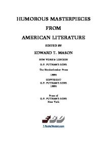
45. If from the Arch aD given the Sine AB was required; I extract the Root of the Equation {x 1 -lox> found above, viz. z.= X I ~.X7 (it being fuppofed that AB x, aD z. and Aa= I) by which I find x=z -{z3 7 9 &c _~Z5 110 50+0 Z J62.880 Z • 46. And moreover if the Coline A{3 were required from that Arch given, make A{3 (= ../1 - xx) -I _I z~ _L " ' r , , , ... Z + _ _7~Z6 10
+
_ 1_ _
A
B
+
=
+ +
+
=
I
+
_I_
4oT"i" o ZS -
J
T6-;FsooZ O,
&c.
Newton's series for sine and cosine (1669) 00
For good measure, Newton included the series forcosz
~ (-1)
k
= £.. -k)1 (Z k=O
2k
In
2 .
the words of Derek Whiteside, "These series for the sine and cosine ... here appear for the first time in a European manuscript" [19].
NEWTON
19
To us, this development seems incredibly roundabout. We now regard the sine series as a trivial consequence of Taylor's formula and differential calculus. It is so natural a procedure that we expect it was always so. But Newton, as we have seen, approached this very differently. He applied rules of integration, not of differentiation; he generated the sine series from the (to our minds) incidental series for the arcsine; and he needed his complicated inversion scheme to make it all work. This episode reminds us that mathematics did not necessarily evolve in the manner of today's textbooks. Rather, it developed by fits and starts and odd surprises. Actually that is half the fun, for history is most intriguing when it is at once Significant, beautiful, and unexpected. On the subject of the unexpected, we add a word about Whiteside's qualification in the passage above. It seems that Newton was not the first to discover a series for the sine. In 1545, the Indian mathematician Nilakantha (1445-1545) described this senes and credited it to his even more remote predecessor Madhava, who lived around 1400. An account of these discoveries, and of the great Indian tradition in mathematics, can be found in [20] and [21]. It is certain, however, that these results were unknown in Europe when Newton was active. We end with two observations. First, Newton's De ana/ysi is a true classic of mathematics, belonging on the bookshelf of anyone interested in how calculus came to be. It provides a glimpse of one of history's most fertile thinkers at an early stage of his intellectual development. Second, as should be evident by now, a revolution had begun. The young Newton, with a skill and insight beyond his years, had combined infinite series and fluxional methods to push the frontiers of mathematics in new directions. It was his contemporary, James Gregory (1638-1675), who observed that the elementary methods of the past bore the same relationship to these new techniques "as dawn compares to the bright light of noon" [22]. Gregory's charming description was apt, as we see time and again in the chapters to come. And first to travel down this exciting path was Isaac Newton, truly "a man of extraordinary genius and proficiency."
CHAPTER 2
Leibniz
Gottfried Wilhelm leibniz
Calculus may be unique in havmg as its founders two individuals better known for other things. In the public mind, Isaac Newton tends to be regarded as a physicist, and his cocreator, Gottfried Wilhelm Leibniz (1646-1716), is likely to be thought of as a philosopher. This is bmh annoying and flattering-annoying in its disregard for their mathematical contributions and flattering in its recognition that it took more than Just an ordinary genius to launch the calculus. Leibniz, with his vaned interests and far-reaching contributions, had an intellect of phenomenal breadth. Besides philosophy and mathematics. he excelled in history, jurisprudence. languages, theology, logic, and diplomacy. When only 27, he was admitted to Londons Royal Society for inventing a mechanical calculator that added, subtracted, multiplied, and divided-a machine that was by all accounts as revolutionary as it was complicated [11.
20
LEIBNIZ
2[
Like Newton, Leibniz had an intense penod of mathematical actiVIty, although his came later than Newton's and in a different country. Whereas Newton developed his fluxional ideas at Cambridge in the mid-1660s, Leibniz did his groundbreaking work while on a diplomatic mission to Paris a decade later. This gave Newton temporal priority-which he and his countrymen would later assert was the only kind that mattered-but it was Leibniz who published his calculus at a time when the De analysi and other Newtonian treatises were gathering dust in manuscript form. Much has been written about the ensuing dispute over which of the two deserved credit for the calculus, and the story is not a pretty one [2]. Modern scholars, centuries removed from passions both national and personal, recognize that the discoveries of Newton and Leibniz were made independently Like an idea whose time had come, calculus was "in the air" and needed only a remarkably penetrating and integrative mind to bring it into existence. This Newton had. Just as surely, so did Leibniz. Upon his arnval in Paris in 1672, he was a nOVIce who admitted to lacking "the patience to read through the long series of proofs" necessary for mathematical success [3]. Dissatisfied with his modest knowledge, he spent time filling gaps, reading mathematicians as venerable as Euclid (ca. 300 BeE) or as up-to-date as Pascal (1623-1662), Barrow, and his sometime-mentor, Chnstiaan Huygens (1629-1695). At first it was hard going, but Leibniz persevered. He recalled that, in spite of his deficiencies, "it seemed to me, I do not know by what rash confidence in my own ability, that I might become the equal of these if I so desired" [4]. Progress was breathtaking. He wrote in one memorable passage that soon he was "ready to get along without help, for I read [mathematics] almost as one reads tales of romance" [5]. After absorbing, almost inhaling, the work of his contemporaries, Leibniz pushed beyond them all to create the calculus, thereby earning himself mathematical immortality And, unlike Newton across the English Channel, Leibniz was willing to publish. The first pnnted version of the calculus was Leibnizs 1684 paper bearing the long title, "Nova methodus pro maximis et minimis, itemque tan-
gentibus, quae nee fraetas, nee irrationales quantitates moratur; et singulare pro illis calculi genus." This translates into "A New Method for Maxima and Minima, and also Tangents, which is Impeded Neither by Fractional Nor by Irrational Quantities, and a Remarkable Type of Calculus for This" [6]. With references to maxima, minima, and tangents, it should come as no surprise that the article was Leibniz's introduction to differential calculus. He followed it two years later with a paper on integral calculus. Even at that early stage, Leibniz not only had organized and codified many of the
22
CHAPTER 2
basic calculus rules, but he was already using dx for the differential of x and Jx dx for its integral. Among his other talents was his ability to provide what laplace later called "a very happy notation" [7].
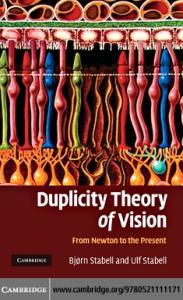
MENSIS OcrOBRlSA. MDC LXXXIV. ....67 NOPA METHQDPS
PRO
ET
MAXIMIS
MI.
ni1fJM, it~11I'jue tA1I!.entiQru, 'j'U n~c frill/1M, 1Itcirrati'lIala 'jUII1Ititiltn mOTatlir~ eIji1lgulareprtJ HIM c"Ie"ligrnus, prr G.G. L. SftaxisAX,&curva:plures,llt VV, ww, yy,ZZ, quarum ordi. natz, ad axem nonnales, VX, W X, YX, ZX, quz vocenrur refpec!tive, v, vv, y, z; &: ipfa AX abfltiifa ab axe, voc:etur x. Tangentes fHlt VB, WC, YD, ZE axi occurrentes refped:ive in punClis B, C, 0 , E. J3m reela aliqNa pro arbitrio aifumta vocerur dx, &: rella quz ftt ad dx, lit v (vel vv, vel y, vel z) eftad VB (vel \'Q'C, vel YO, vel ZE) vo· eetur d v (vel d vv, vel dy vel dz) five differenfia ipfarum 'tI (vel ipfa. rum YV, aut y, aut z) His pofitis calculi regulz erunt tales : _ Sira quantitas data conftans, erit t'la zqualls 0, & d ax erit zqu' adx: li fity zqu. 'tI (feu ordinata quzvis curvz YY, zClualis cuiyis or·· dinatz refpondenti curva: VV) erit dy zqu. dp. Jam AJditio £5 SIIbt,....l1itJ:(i lit z ·yt yvt x zqu. v, erit dz·-ytvvtx feu dp, zqu. dz -dytdvvt dx. MliltiplieAti., ~zqu.xd'tltvdx, feu pofttO y a:qu. XP, tiet d y zqu. x d P t p d x. In arbitrio enim eft vel formulam, ut X" vel compendio pro ea literam, ut y, adhibere. Notandum &: x &: dx eodem modo in hoc calculo trad:ari,ut y & dy,vel aliam literam indeterminatam cum fua differentiali. Notandum etiam nOn dari temper regrelfum a differentiali .Equation" nifi cum quadam cautioJI ftC, de quo alibi.
.Porro Di,ijo, d-vcl (poGto Z lIequ.
TAl.
xu
,
) d z z'lu,
tpdytyd, Leibniz5 first paper on differential calculus (1684)
In this chapter, we examine a pair of theorems from the years 16731674. Much of our discussion is drawn from Leibniz's monograph Historia et origo calculi differentialis, an account of the events surrounding his creation of the calculus [8]. Our first result, more abstract, is known as the transmutation theorem. Although its geometrical convolutions may not appeal to modern tastes, it reveals his mathematical gift and leads to an early version of what we now call integration by parts. The second result,
23
LEIBNIZ
a consequence of the first, is the so-called "Leibniz Series." Like Newton's work, discussed in the preVIous chapter, this combined series expansions and basic integration techniques to produce an important and fascinating outcome.
THE TRANSMUTATION THEOREM
Finding areas beneath curves was a hot topic in the middle of the seventeenth century, and this is the subject of the Leibniz transmutation theorem. Suppose, in figure 2.1, we seek the area beneath the curve AB. Leibniz imagined this region as being composed of infinitely many "infinitesimal" rectangles, each of WIdth dx and height y, where the latter varies with the shape of AB. To us today, the nature of Leibniz's dx is unclear. In the seventeenth century, it was seen as a least possible length, an infinitely small magnitude that could not be further subdivided. But how is such a thing possible? Clearly any length, no matter how razor-thin, can be split in half. Leibniz's explanations in this regard were of no help, for even he became
___-B y=y(x)
A
y
.. x
---+-------~---------
dx
Figure 21
24
CHAPTER 2
unintelligible when addressing the matter. Consider the followmg passage from sometime after 1684: by ... infinitely small, we understand something ... indefinitely small, so that each conducts itself as a sort of class, and not merely as the last thing of a class. If anyone wishes to understand these [the infinitely small] as the ultimate things ... , it can be done, and that too WIthout falling back upon a controversy about the reality of extensions, or of infinite continuums in general, or of the infinitely small, ay even though he think that such things are utterly impossible. [9] The reader is forgiven for finding this clarification less than clanfymg. Leibniz himself seemed to choose expediency over logic when he added that, even if the nature of these indivisibles is uncertain, they can nonetheless be used as "a tool that has advantages for the purpose of the calculation." Again we glimpse the mathematical quagmire that would confront analysts of the future. But in 1673 Leibniz was eager to press on, and a later generation could tidy up the logic. Returning to figure 2.1, we see that the infinitesimal rectangle has area y dx. To calculate the area under the curve AB, Leibmz summed an infinitude
___- B
",
T
","'a
D
",
W
",'"
",4
",'"
1
1 I
\
Iy I
z
\
\h \
\ \ \a \ \
x
I I I I I
o
dx
Figure 2 2
25
LEIBNIZ
of these areas. As a symbol for this process, he chose an elongated "s" (for "summa") and thus denoted the area as f y dx. Thereafter, his integral sign became the "logo" of calculus, announcing to all who saw it that higher mathematics was afoot. It is one thing to have a notation for area and quite another to know how to compute it. Leibniz's transmutation theorem was aimed at resolving this latter question. His idea is illustrated in figure 2.2, which again shows curve AB, the area beneath which is our object. On the curve is an arbitrary point P with coordinates (x, y). At P, Leibmz constructed the tangent line t, meeting the vertical axis at point TWlth coordinates (0, z). Leibmz explained this construction by noting that "to find a tangent means to draw a line that connects two points of the curve at an infinitely small distance" [10]. Letting dx be an infinitesimal increment in x, he then created an infinitely small right tnangle with hypotenuse PQ along the tangent line and haVIng sides of length dx, dy, and ds, an enlargement of which appears in figure 2.3. We let ex be the angle of inclination of this tangent line. Leibniz stressed that, "Even though this triangle is indefinite (being infinitely small), yet ... it was always possible to find definite triangles similar to it" [11]. Of course, one may wonder how an infinitely small tnangle can be similar to anything, but this is not the time to quibble. Leibniz regarded tiTOP in Figure 2.2 as being similar to the infinitesimal
dy
triangle in figure 2.3. It followed that to get dx
Y- z = -PO = --, which he solved TO
x
dy z=y-x-.
(1)
dx
Q
dy
p
dx
Figure 2.3
26
CHAPTER 2
Next, Leibniz extended his tangent line PT leftward, and from the origin drew segment OW of length h perpendicular to this extension (again, see figure 2.2). Because L.PTD has measure a, we know that LOTW has measure 1r - a, and so the measure of LTOW is a as well. This makes .6.0TW similar to the infinitesimal triangle, and so we generate another
.
z
ds
.
propomon h = dx' from WhICh we conclude that hds=zdx.
(2)
Leibniz then drew .6.0PQ radiating from the origin and having as base the hypotenuse PQ of the infinitesimal triangle. In order not to clutter figure 2.2 any further, we redraw the diagram, with this particular triangle, in figure 2.4. By now, the reader may suspect that Leibniz was adrift, lost in a sea of pOintless triangles. But in fact the oblique, infinitesimal triangle OPQ was central to his transmutation theorem. Because its base is of length PQ = ds 1
~
and its height is OW = h, we see that its area is -h ds, which, by (2) above, 1 2 isjust-zdx. 2 Leibniz assembled an infinitude of these infinitesimal triangles, all radiating from the ongin and terminating along AB, as shown in figure 2.5.
~_-B
-'
w , ,4
,,
,, ,, ,,
'h
x
o
dx
Figure 2.4
LEIBNIZ
27
Writing years later, Leibniz remembered that he "happened to have occasion to break up an area into triangles formed by a number of straight lines meeting in a point, and ... perceived that something new could be readily obtained from it" [12J. This polar perspective was critical, for Leibniz recognized that the area of the wedge in figure 2.5 was the sum of the areas of infinitesimal triangles whose analytic expression he had determined above. That is, Area (wedge) = Sum of tnangular areas = f
1 1 z dx =
f z dx.
(3)
In truth, Leibniz was not primanly interested in the area of this wedge.
f
Rather, he sought the area under curve AB in figure 2.1, that is, y dx. Fortunately it takes only a bit of tinkenng to relate the areas in question, for the geometry of figure 2.6 shows that Area under curve AB = Area (wedge) + Area
(~ObB) -
Area
(~OaA).
This relationship, by (3), has the symbolic equivalent
f ydx
= ..!.fzdx +..!.b y(b) - ..!.ay(a).
(4)
2 2 2 Here at last is the transmutation theorem. The name indicates that the original integral f y dx has been transformed (or "transmuted") into a sum
~-7B
Figure 2.5
28
CHAPTER 2
B
_ _-"1
Y =y(x)
1 1 I 1 1 I I I I y(b)
I
I 1 1 I I I 1 1
b
Figure 2.6
1 of the new integral "2
f z dx and the constant "21 b y(b) - "21 a yea). Today
we might find it more palatable to insert limits of integration (a notational deVlce Leibniz did not employ) and recast the theorem as
. Jabydx = -21 Jba zdx+-21 [ xyl bJ a
(5)
Formula (5) is notable for at least two reasons. First, it is possible that the "new" integral in z may be easier to evaluate than the original one in y. If so, z would play an auxiliary role in finding the original area. For seventeenth century mathematiCians, a curve playing such a role was called a quadratrix, that is, a facilitator of quadrature. If it produced a simpler integral, then this whole, long process would payoff. As we shall see in a moment, this is exactly what happened in the derivation of the Leibniz series. The relationship in (5) has a theoretical significance as well. Recall that z = z(x) was the y-intercept of the line tangent to the curve AB at the point (x, y). The value of z thus depends on the slope of the tangent line and so injects the derivative into this mix of integrals. One senses that an important connection is lurking in the wings.
29
LEIBNIZ
To see it, we recall from (1) that z Then, returning to (4), we have
=y -
dy x - and so z dx = y dx - x dy.
dx
1 y(b) - -ay(a) 1 f ydx = -21 f zdx + -b 2 2 I y(b) - -ay(a) I = -I f [ydx - xdy] + -b 2 2 2 I I = -If ydx--If xdy+-by(b)--ay(a) 2 2 2 2 ' which we solve to conclude that fy dx = b y(b) - a yea) - fx dy. Again, limits of integration can be inserted to give
f y dx = b
a
X
y
b I a
fY(b) y(a)
(6)
xd y.
The geometric validity of (6) is evident in figure 2.7, for area of the region with vertical strips, whereas
s: y dx is the
J;(~: x dy is the area of that
with horizontal strips. Their sum is clearly the difference in area between the outer rectangle and the small one in the lower left-hand corner. That is,
f ydx+ b
a
fY(b) y(a)
xdy=by(b)-ay(a),
which can be rearranged into (6). There is something else about (6) that bears comment: it looks familiar. So it should, because it follows easily from the well-known scheme for integration by parts
f:
f(x)g'(x)dx
= f(x)
g(x)l: -
f:
g(x) j'(x)dx,
if we specify g(x) = x and f(x) = y. In that case g' (x) = 1 and j'(x)dx = dy, and a substitution converts the integration-by-parts formula into the transmutation theorem. After all of Leibniz's convoluted reasoning with its infinitesimals and tangent lines, its similar triangles and wedge-shaped areas-in short, after a most circuitous mathematical Journey-we arrive at an instance of integration by parts, a calculus superstar making an early and unexpected entrance onto the stage. This was intriguing, but Leibniz was not finished. By applying his transmutation theorem to a well-known curve, he discovered the infinite senes that still carries his name.
30
CHAPTER 2
-'I'
--
B
y(b) ~------------------ - , y=y(x)
/ y(a)
~"'"
------7/ AI
I I I I I I
I I I I I I I I I I I I
a
0
,
b
Figure 2 7 THE LEIBNIZ SERIES
Leibniz began with a circular arc. Specifically, he considered a circle of radius 1 and center at (1, 0) and let the curve AB from his general transmutation theorem be the quadrant of this circle shown in figure 2.8. As will become evident momentarily, it was an inspired choice. The circle's equation is (x - 1)2 + y2 = lor, alternately, x 2 + y2 = 2x. From the geometry of the situation, it is clear that the area beneath the quadrant is n/4, and so by (1) and (5) we have -n = 4
11 Y dx = -1 x yII + -1 11 z dx ° 2 ° 20 '
where
z = y - x -dy. dx
Using his newly created calculus, Leibniz differentiated the circles equation to get 2x dx + 2y dy
dy
1- x
= 2 dx, and so dx = -y-' This led to the simplification
Z= Y - x ~ = Y _
f ~ +:'x] =
y'
x =
2X; x = ~
Leibniz's objective was to find an expression for x in terms of the quadratrix z, and so he squared the previous result and again used the equation of the circle to get
31
LEIBNIZ
y=V2x-x 2
x
a Figure 2 8
Z
2
2
2
X = -X = --~ = 2
l
2x - x
2
X
2- x '
The challenge was to evaluate
which he solved for x
= -2Z -2 . 1+ z
(7)
J>dx, the shaded area in figure 2.9. A ~
look at the graph of the quadratrix z = x and an observation similar 2-x to the one above shows that
J~ z
dx = Area (shaded region) = Area (square) -
Area (upper region)
= 1 - f~ x dz.
(8)
Returning to the transmutation theorem, Leibniz combined (7) and (8) as follows:
-n = -Ixyll + -1 11 z dx = -1 + -1 [ 1 4
2
020
II
22
11 x dz ]
2
0
Z2 = 1--1 -2z - d z = 1- 11 --dz.
2
0
1 + Z2
0
1 + Z2
32
CHAPTER 2
z
z=
J2~X
L . . . - - - - -......
o
X
Figure 2.9
He rewrote this last integrand as
1]
-Z2- = z2[- - = z2[1- z2+ z4- z6+ 1 + Z2
1 + Z2
= Z2
_ Z4
+ Z6
- Z8
+.
0
0
0
0
oj
,
where a geometric series has appeared within the brackets. From this, Leibniz concluded that l !!.- = 1- r [z2 - Z4 + Z6 - Z8 + ojdz 4 Jo 0
=1- [ ; -7C = 1 4
1
3
1, then
1
3
6
10
15
b
bd
bd
bd
bd
T:=-+-+-+-+-+···= 2 3 4
d3 bed _1)3 .
Proof: The trick is to break T into a string of geometric series and exploit
the fact that the kth triangular number is 1 + 2 + 3 + ... + k:
1
1
1
1
1
b
bd
bd
bd
bd
=--lib - Ilbd bed - 1) ,
2 bd
2 bd
2 bd
2 bd
(2lbdi 2 =--2 21bd - 21bd bed - 1) ,
3 bd
3 bd
3 bd
C3lbd 2 i 3 =--2 3 31bd - 31bd bd(d -1) ,
4 bd
4 bd
(4lbd 3 i 4 =---3 4 2 41bd - 41bd bd (d - 1) ,
- + - + -2 + -3+ - 4+ ... = - + -2+ - 3+ - + ... = 4 -+ -+ -+ ... = 2 3 4 -+ -+ ... = 3 4
=
d
(llb)2
=
44
CHAPTER 3
Adding down the columns gives 1 1+2 1+2+3 1+2+3+4 -+--+ + + ... b bd bd 2 bd 3 3 4 = d + 2 + + 2 + .... bed -1) bed - 1) bd(d - 1) bd (d - 1)
In other words, T
= _d_ [.!. + ~ + -.2..-2 + ---±-3 + ...J d- 1 b
bd
bd
bd
d d d2 d3 =--N=--x =--d- 1 d - 1 bed - Ii bed _1)3 ' by theorem N.
Q.E.D.
1 3 6 10 15 For example, WIth b = 2 and d = 4, we have - + - + - + - + - + 2 8 32 128 512 32 27 Jakob then considered pyramidal numbers in the numerators. 1 b
4 10 20 35 + - 2 + - 3 + - 4 + ... bd bd bd bd
Theorem P: If d > 1 x then P == - + -
,
=
d4 bed - 1)4 . Proof: This follows easily because
3
Hence (1 -
4
.!.Jp =T= d and so P = __d_ d bed - 1)3 ' bed - 1)4 .
As an example, with b = 5 and d = 5, we have
_
Q.E.D.
45
THE BERNOULLIS
Jakob finished this part of the Tractatus by considering infinite series WIth the cubic numbers in the numerators and a geometnc progression in the denominators. 1 8 27 64 125 Theorem C: If d > 1 then C = - + - + + -3+ - 4+ ... 2
,
2
b
bd
bd
bd
bd
=
2
d Cd + 4d + 1) bCd _1)4 Proof:
When Jakob let b = 2 and d = 2, he concluded that
i £ = ~ +~ + k=!
2k
2
4
27 + 64 + 125 + 216 8 16 32 64
+ 343 + 512 + 729 + 1000 + ... = 26 128
256
512
1024
exactly, surely a strange and nonintuitive result. After such successes, Jakob Bernoulli may have begun to feel invincible. If he entertained such a notion, he soon had second thoughts, for the senes of reciprocals of square numbers, that is,
i ~,
resisted all his k efforts. He could show, using what we now recognize as the comparison test, that the series converges to some number less than 2, but he was unable to identify it. Swallowing his pride, Jakob included this plea in his Tractatus: "If anyone finds and communicates to us that which has thus far eluded our efforts great WIll be our gratitude" [16]. k=!
46
CHAPTER 3
As we shall see, Bernoulli's challenge went unmet for a generation until finally yielding to one of the greatest analysts of all time. Jakob Bernoulli was a master of infinite senes. His brother Johann, equally gifted, had his own research interests. Among these was what he called the "exponential calculus," which will be our next stop.
JOHANN AND XX
In a 1697 paper, Johann Bernoulli began WIth the following general rule: "The differential of a logarithm, no matter how composed, is equal to the differential of the expression diVIded by the expression" [17]. For instance, d[ln(x)] d[ln
= dx x
or
~(xx + yy)] = ~d[ln(xx + yy)] = ~[2Xdx + 2YdY] 2
2
xx + yy
xdx+ ydy =-_....=....-.=.... xx+ yy We have retained Bernoullis onginal notation for this last expression. At that time in mathematical publishing, higher powers were typeset as they are today, but the quadratic x 2 was often written xx. Also, in the interest of full disclosure, we observe that Bernoulli denoted the natural logarithm ofx by Ix. Johann wrote the corresponding integration formula as
Jdxx = Ix.
Early in his career he had been seriously confused on this point, believing that -dx = x ldx = -1 XO = -1 x 1 = 00, an overly enthusiastic application x 0 0 of the power rule and one that has yet to be eradicated from the repertoire of beginning calculus students [18]. Fortunately,Johann corrected his error. With these preliminaries behind him, Johann promised to apply principles "first invented by me" to reap a rich harvest of knowledge "incrementing this new infinitestimal calculus WIth results not previously found or not WIdely known" [19]. Perhaps his most interesting example was the curve y = xx, shown in figure 3.2. For an arbitrary point F on the curve, Johann sought the subtangent, that is, the length of segment LE on the x-axis beneath the tangent line. To do this, he first took logs of both sides: In(y) = In(xx) = x In(x). He then used his rule to find the differentials:
J J-
47
THE BERNOULLIS
~
/ / / /
/ / / / / / /
/
Y
/ /
/ / / / /
M
L
E
Figure 3 2
1
-dy
y
dx
= x - + lnxdx = 0 + lnx)dx. x
y But - = slope of tangent line LE length of the subtangent LE
~ = dx = yO + In x),
= (
YI) y 1 + nx
and he solved for the
1 1 + lnx
Bernoulli next sought the minimum value-what he called the "least of all ordinates"-for the curve. This occurs when the tangent line is horizontal or, equivalently, when the subtangent is infinite. Johann described a somewhat complicated geometric procedure for identifying the value of x for which 1 + In x = 0 [20]. His reasoning was fine, but the form of his answer seems, to modern tastes, less than optimal. Johann was hampered because the introduction
48
CHAPTER 3
of the exponential function still lay decades in the future, so he lacked a notation to express the result simply We now can solve for x = lie and conclude that thelm1i~}:num value of xx, that is, the length of segment eM ~
in figure 3.2, is
a number roughly equal to 0.6922. This
= _1_,
ifC
e
answer, it goes without saying, is by no means obvious. Johann was just warming up. In another paper from 1697, he tackled a tougher problem: finding the area under his curve y = XX from x = 0 to
p
x
x = 1. That is, he wanted the value of Jo x dx. Remarkably enough, he found what he was seeking [21]. The argument required two preliminaries. The first he expressed as follows: Z2
If z = In N, then N = 1 + z + -
2
Z3
Z4
2x3
2x3x4
+-- +
+ ....
Here we recognize the expression for N as th~ exponential series. If N =xx, then Z = In N = x In x, and Johann deduced that x 1 I x 2(lnx)2 x\lnx)3 x 4(lnx)4 + + +.... (3) x = + x nx + 2
2x3
2x3x4
His objective was to integrate this sum by summing the individual
fxk(ln
integrals, and for this he needed formulas for
x)kdx. He proceeded
recursively to generate the table shown on this page.
fdx
=." 0" to the phrase "as little as one wishes." Yet this was an advance of the first order. Cauchys idea, based on "closeness," avoided some of the pitfalls of earlier attempts. In particular, he said nothing about reaching the limit nor about surpassing it. Such issues ensnared many of Cauchy's predecessors, as Berkeley had been only too happy to point out. By contrast, Cauchys so-called "limit avoidance" definition made no mention whatever of attaining the limit, Just of getting and staying close to it. For him, there were no departed quantities, and Berkeley's ghosts disappeared. Cauchy introduced a related concept that may raise a few eyebrows. He wrote that "when the successive numerical values of a variable decrease indefinitely (so as to become less than any given number), this variable will be called ... an infinitely small quantity" [5]. His use of "infinitely small" strikes us as unfortunate, but we can regard this definition as Simply spelling out what is meant by convergence to zero. Cauchy next turned his attention to continuity. Intuition might at first suggest that he had things backwards, that he should have based the idea of limits upon that of continuity and not vice versa. But Cauchy had it right. Reversing the "obvious" order of affairs was the key to understanding continuous functions. Starting WIth y =J(x), he let i be an infinitely small quantity (as defined above) and considered the functions value when x was replaced by x + i. This changed the functional value from y to y + i1y, a relationship Cauchy expressed as y + i1y
=J(x + i)
or
=J(x + i) - J(x) i1y =J(x + i) - J(x)
i1y
If, for i infinitely small, the difference was infinitely small as well, Cauchy called J a continuous function of x [6]. In other
79
CAUCHY
words, a function is continuous at x if, when the independent variable x is augmented by an infinitely small quantity, the dependent variable y likewise grows by an infinitely small amount. Again, reference to the "infinitely small" means only that the quantities have limit zero. In this light, we see that Cauchy has called j continuous at x if lim[J(x + i) - j (x) I = 0, which is equivalent to the modern definition, i---)O
limj(x + i) i---)O
= j(x).
As an illustration, Cauchy considered y = sin x [71. He used the fact that lim (sin x) = 0 as well as the trig identity sin(a + f3) - sina = 2 sin({312) .
x---)o
cos(a + {312). Then, for infinitely small i, he observed:
l'1y
=j(x + i) -
j(x)
=sin(x + i) -
sin x = 2sin(il2)cos(x + il2).
(1)
Because il2 is infinitely small, so is sin(il2) and so too is the entire righthand side of (I). By Cauchys definition, the sine function is continuous at any x. We note that Cauchy also recognized one of the most important properties of continuous functions: their preservation of sequential limits. That is, if j is continuous at a and if {xk} is a sequence for which lim xk = a, then k---)oo
it follows that lim j(x k ) = j[lim xkJ k---)oo k---)oo
= j(a). We shall see him exploit this
principle shortly. He then considered "derived functions." For Cauchy, the differential quotient was defined as j(x + i) - j(x) -l'1y = "--------"'---
I'1x
where i is infinitely small. Taking his notation from Lagrange, Cauchy denoted the derivative by y' or r(x) and claimed that this was "easy" to determine for simple functions like y
= r ± x, rx, rlx, x r , AX, 10gA x, sin x, cos x, arcsin x, and arccos x.
We shall examine just one of these: y = 10gA x, the logarithm to base A > 1, which Cauchy de~oted by L(x) [8].. . l'1y _ j(x + i) - j(x) He began wIth the dIfferentIal quotIent I'1x i = L(x + i) - L(x)
- - - - - - for i infinitely small and introduced the auxiliary variable
80
a
i
=-, x
CHAPTER 6
which is infinitely small as well. Using rules of logarithms and
substituting liberally, Cauchy reasoned that L(x + i) - L(x) =
L(XX+
i)
L(x +x
ax
= ---"
) 0-.
ax 1
-LO + a) a
x
= ~LO + a)lIa.
(2)
x
1 For a infinitely small, he identified this last expression as - LCe). Today we x would invoke continuity of the logarithm and the fact that limO + a)l!a = e a~O
to justify this step. In any case, Cauchy concluded from (2) that the derivative 1 of L(x) was - L(e). As a corollary, he noted that the derivative of the natural x 1
logarithm In(x) is -In(e)
x
1
= -. x
He obviously had his differential calculus well under control.
THE INTERMEDIATE VALUE THEOREM
Cauchy's analytic reputation rests not only upon his definition of the limit. At least as significant was his recognition that the great theorems of calculus must be proved from this definition. Whereas earlier mathematicians had accepted certain results as true because they either conformed to intuition or were supported by a diagram, Cauchy seemed unsatisfied unless an algebraic argument could be advanced to prove them. He left no doubt of his position when he wrote that "it would be a serious error to think that one can find certainty only in geometrical demonstrations or in the testimony of the senses" [9]. His philosophy was evident in a demonstration of the intermediate value theorem. This famous result begins with a function f continuous between X o and X (Cauchy's preferred designation for the endpoints of an interval). If f(x o) < 0 and f(X) > 0, the intermediate value theorem asserts that the function must equal zero at one or more points between X o and x. For those who trust their eyes, nothing could be more obvious. An object moving continuously from a negative to a positive value must
CAUCHY
81
somewhere slice across the x-axis. As indicated in figure 6.1, the intermediate value occurs at x = a, where fCa) = O. It is tempting to ask. "What's the big deal?" Of course, the big deal is that mathematicians hoped to free analysis from the danger of intuition and the allure of geometry. For Cauchy, even obvious things had to be proved with indisputable logic. In that spint, he began his proof of the intermediate value theorem by letting h =X - Xo and fixing a whole number m > 1 [10]. He then broke the interval from X o to X into m equal subintervals at the points x o, X o + him, Xo + 2h1m, ... , X - him, X and considered the related sequence of functional values: fCxo),fCx o + hlm),fCxo + 2h1m), ... ,fCX - hlm),fCX). Because the first of these was negative and the last positive, he observed that, as we progress from left to right, we will find two consecutive functional values with opposite signs. More precisely, for some whole number n, we have
fCx o + nhlm)
~
0
but fCx o + Cn + 1)hlm) ~ O.
We follow Cauchy in denoting these consecutive points of subdivision by + nhlm == Xl and Xo + Cn + 1)hlm == Xl' Clearly, Xo ~ Xl < Xl ~ X, and the length of the interval from Xl to Xl is him. He now repeated the procedure across the smaller interval from Xl to Xl' That is, he divided it into m equal subintervals, each of length him 2 , and considered the sequence of functional values Xo
y=f(x)
Figure 6.1
82
CHAPTER 6
Again, the leftmost value is less than or equal to zero, whereas the rightmost is greater than or equal to zero, so there must be consecutive points x2 and X2 a distance of hlm 2 units apart, for which j(x2) ~ 0 and j(X2) ~ o. At this stage, we have Xo ~ Xl ~ X2 < X2 ~ Xl ~ X. Those familiar with the bisection method for approximating solutions to equations should feel perfectly at home with Cauchy's procedure. Continuing in this manner, he generated a nondecreasing sequence Xo ~ Xl ~ X2 ~ X3 ~ . . . and a nonincreasing sequence··· ~ X3 ~ X2 ~ Xl ~ X, where all the values j(xh) ~ 0 and j(Xh) ~ 0 and for which the gap X h - Xh = hlmh. For increasing k, this gap obviously decreases toward zero, and from this Cauchy concluded that the ascending and descending sequences must converge to a common limit a. In other words, there is a point a for which lim Xh = a = lim X h. h~~ h~~ We pause to comment on this last step. Cauchy here assumed a version of what we now call the completeness property of the real numbers. He took it for granted that, because the terms of the sequences {Xh} and {Xh } grow arbitrarily close to one another, they must converge to a common limit. One could argue that his belief in the existence of this point a is as much a result of unexamined intuition as simply believing the intermediate value theorem in the first place. But such a judgment may be overly harsh. Even if Cauchy invoked an untested hypothesis, he had at least pushed the argument much deeper toward the core principles. If he failed to clear the path of all obstacles, he got rid of most of the brush underfoot. To finish the argument, Cauchy stated (without proof) that the point a falls within the original interval from Xo to X, and then he used the continuity of j to conclude, in modern notation, that j(a)
= j [lim Xh] = lim j(xh) ~ 0
j(a)
= j[lim x h] = lim j(Xh ) ~ o.
h~oo
h~~
h~oo
and
k~~
In Cauchy's words, these inequalities established that "the quantity j(a) ... cannot differ from zero." He had thus proved the existence of a number a between Xand X for which j(a) = O. The general version of the
intermediate value theorem, namely that a continuous function takes all values betweenj(xo) andj(X), follows as an easy corollary. This was a remarkable achievement. Cauchy had, for the most part, succeeded in demonstrating a "self-evident" principle by analytic methods.
CAUCHY
83
As Judith Grabiner observed, "though the mechanics of the proof are sim-
ple, the basic conception of the proof is revolutionary. Cauchy transformed the approximation technique into something entirely different: a proof of the existence of a limit" [11].
THE MEAN VALUE THEOREM
We now turn to another staple of the calculus, the mean value theorem for derivatives [12]. In his Calcul infinitesimal, Cauchy began with a preliminary result. Lemma: If, for a function f continuous between X o and X, one lets A be the smallest and B be the largest value that l' takes on this interval, then A~f(X)- fCxo)~B.
X-x o Proof: We note that Cauchy's reference to l'-and thus his unstated assumption that f is differentiable-would of course guarantee the continuity of f. Moreover, he assumed outright that the derivative takes a greatest and least value on the interval [xo, X]. A modern approach would treat these hypotheses with more care. If his statement seems peculiar, his proof began with a nowfamiliar ring, for Cauchy introduced two "very small numbers" 0 and E. These were chosen so that, for all positive values of i < 0 and for any x between Xo and X, we have
f 'C X ) -
E
< fCx + i) - fCx) < f'C) X + E. i
(3)
Here Cauchy was assuming a uniformity condition for his choice of o. The existence of the derivative certainly means that, for any E> 0 and for any fixed x, there is a 0> 0 for which the inequalities of (3) hold. But such a 0 depends on both E and the particular point x. Without additional results or assumptions, Cauchy could not justify the choice of a single 0 that simultaneously works for all x throughout the interval. Be that as it may, he next subdivided the interval by choosing points X o < Xl
< x 2 < ... < x n- l < X,
84
CHAPTER 6
where Xl - X O, X 2 - Xl' . . . , X - x n- 1 "have numerical values less than 0." For these subdivisions, repeated applications of (3) and the fact that A ~ j'ex) ~ B imply that
A-
£
< j'ex n - 1)
-
£
1, k=l
k---7 OO
then the series converges. Proof: As with the root test, Cauchy sought a "buffer" between 1 and hand so chose a real number a WIth 1 < a < h. This guaranteed the existence
94
CHAPTER 6
In(u k )
of a positive integer m so that In(l/k) > a for all k ~ m. From there, he observed that In(u
)
a < - - kIn(l/k)
-In(u
)
k = ---"-
In k
and so
a In(k) < In(
:k J
Exponentiating both sides of this inequality, he deduced that kG < -
1
Uk
1
and so Uk < -; for all k ~ m. But
k
~
1
1-; (which is now called a p-series) k
h=m
~
converges because a > 1, and so the origInal senes
I
Uk
converges by
k=I
the comparison test.
Q.E.D.
As an example, consider
~
In(k)
k=!
kP
1--, where p > 1. Cauchys test requires us
In[ln(k)/kP] I ( k) , which suggests in tum that we first simplify the k--+~ n 1/
to evaluate lim
quotient: In[ln(k)/kP] In(lIk)
=
In[ln(k)] - p In(k) -lnCk)
, ., . (In[lnCk)] By I HospItals rule, ~~ - InCk)
)
=-
In[ln(k)] InCk) + p. .
.
+ p = P > 1, establIshmg the conver-
~ In(k) , gence of £..J - - by Cauchys test. It is a very nice result. k=I
kP
Before leaving Augustin-Louis Cauchy, we offer an apology and a preview. We apologize for a chapter that reads like a precis of an introductory analysis text. Indeed, there is no stronger testimonial to Cauchy's influence than that his "greatest hits" are now the heart and soul of the subject. Building upon the idea of limit, he developed elementary real analysis in a way that remains the model to this day. As Bell properly observed, Cauchy stands at center stage, and it is for this reason that the present chapter is one of the books longest. It could hardly be otherwise. This brings us to the preview. None of these accolades should suggest that, after Cauchy, the quest was finished. On at least three fronts there was still work to be done, work that will occupy us in chapters to come.
CAUCHY
95
First, his definitions could be made more general and his proofs more rigorous. A satisfactory definition of the integral, for instance, need not be limited to continuous functions, and the nagging issue of uniformity had to be identified and resolved. These tasks would fall largely to the German mathematicians Georg Friedrich Bernhard Riemann and Karl Weierstrass, who in a sense supplied the last word on mathematical precision. Second, Cauchy's more theoretical approach to continuity, differentiability, and integrability motivated those who followed to sort out the connections among these concepts. Such connections would intrigue mathematicians throughout the nineteenth century, and their resulting theorems-and counterexamples-would hold plenty of surprises. Finally, the need to understand the completeness property raised questions about the very nature of the real numbers. The answers to these questions, combined with the arrival of set theory, would change the face of analysis, although no mathematician active in 1840 could know that a revolution lay just over the horizon. But any mathematician active in 1840 would have known about Cauchy. On this front, we shall give the last word to math historian Carl Boyer. In his classic study of the history of calculus, Boyer wrote, "Through [his] works, Cauchy did more than anyone else to impress upon the subject the character which it bears at the present time" [20]. In a very real sense, all who followed are his disciples.
CHAPTER 7
Riemann
Georg Fnednch Bernhard Riemann
By
~function~
this point of our story, the had assumed a central imponance in analysis. At first it may have seemed like a straightfOlward, even innocuous notion, but as the colJection of functions grew ever more sophisticated-and ever more strange-mathematicians realized they had a conceptual tiger by the tail. To sketch this evolution, we return briefly to the origins. As we have seen, seventeenth century scholars like Newton and Leibniz believed that the raw material of their new subject was the curve, a concept rooted in the geometridintuitive approach that later analysts would abandon. It was largely because of Euler that attention shifted from curves to functions. This significant change in viewpoint, dating from the publication of his lntroducfio in analysin infinitorum, positioned real analysis as the study of functions and their behavior. 96
RIEMANN
97
Euler addressed this matter early in the Introductio. He first distinguished between a constant quantity (one that "always keeps the same value") and a variable quantity ("one which is not determined or is universal, which can take on any value") and then adopted the following definition: "A function of a variable quantity is an analytic expression composed in any way whatsoever of the variable quantity and numbers or constant quantities" fl]. As examples he offered expressions like a + 3z,az + b~a2 - Z2, and cZ. These ideas were a huge improvement upon the "curve" and represented a triumph of algebra over geometry. However, his definition identified functions with analytic expressions-which is to say, functions with formulas. Such an identification painted mathematicians into some bizarre
x corners. For instance, th e function f()
X = { -x
if x ~ 0, h 'f 0 as s own in
1
x
< ,
figure 7.1 was considered "discontinuous" not because its graph jumped around but because its formula did. Of course, it is perfectly continuous by the modern (i.e., Cauchy's) definition. Worse, as Cauchy observed, we
R.
could express the same function by a single formula g(x) = There seemed to be ample reason to adopt a more liberal, and liberating, view of what a function could be. Euler himself took a step in this direction a few years after providing the definition above. In his 1755 text on differential calculus, he wrote Those quantities that depend on others ... , namely, those that undergo a change when others change, are called functions of
-1
Figure 7.1
98
CHAPTER 7
these quantities. This definition applies rather widely and includes all ways in which one quantity can be determined by others. [2] It is important to note that this time he made no explicit reference to analytic expressions, although in his examples of functions Euler retreated to familiar formulas like y = x 2 . As the eighteenth century became the nineteenth, functions were revisited in the study of real-world problems about vibrating strings and dissipating heat. This story has been told repeatedly (see, for instance, [3] and [4]), so we note here only that a key figure in the evolving discussion was Joseph Fourier. He came to believe that any function defined between -a and a (be it the pOSition of a string, or the distribution of heat in a rod, or something entirely "arbitrary") could be expressed as what we now call a Fourier series:
1 ~( ahcos--+bhsm--, nJrx . nJrx) j(x)=-ao+L. 2
h=l
a
a
where the coefficients ah and bh are given by
ah
nJrx = -1 fa j(x)cos--dx
a
-a
a
1 fa
and bh = a
-a
nJrx
j(x)sin-dx.
a
(1)
To insure that his readers were under no illusions about the level of generality, Fourier explained that his results applied to "a function completely arbitrary, that is to say, a succession of given values, subject or not to a common law," and he went on to describe the values of y =j(x) as succeeding one another "in any manner whatever, and each of them is given as if it were a single quantity" [5]. This statement extended the "late Euler" pOSition that functions could take values at will across different points of their domain. On the other hand, it was by no means clear that the formulas in (1) always hold. The coefficients ah and bh are integrals, but how do we know that integrals of general functions even make sense? At least implicitly, Fourier had raised the question of the existence of a definite integral, or, in modern terminology, of whether a function is or is not integrable. As it turned out, Fourier had badly overstated his case, for not every function can be expressed as a Fourier series nor integrated as required by (1). Further, in practice he restricted himself, as had Euler before him, to examples that were fairly routine and well behaved. If the concept of a truly "arbitrary" function were to catch on, someone would have to exhibit one.
99
RIEMANN
DIRICHLET'S FUNCTION
That somebody was Peter Gustav Lejeune-Dirichlet 0805-1859), a gifted mathematician who had studied with Gauss in Germany and with Fourier in France. Over his career, Dirichlet contributed to branches of mathematics ranging from number theory to analysis to that wonderful hybrid of the two called, appropriately enough, analytic number theory. Here we consider only a portion of Dirichlets 1829 paper "Sur la convergence des series trigonometriques qui servent a representer une jonction arbitrarie entre des Iimites donnees" (On the Convergence of Trigonometric Series that Represent an Arbitrary Function between Given Limits) [6]. In it, he returned to the representability of functions by a Fourier series like 0) and the implicit existence of those integrals determining the coefficients. We recall that Cauchy defined his integral for functions continuous on an interval [a, 13]. Using what we now call "improper integrals," Cauchy extended his idea to functions with finitely many points of discontinuity in [a, f31. For instance, if j is continuous except at a single point r within [a, 13], as shown in Figure 7.2, Cauchy defined the integral as
S:j(x)dx= {j(x)dx+ S: j(x)dx=
li~tj(x)dx+ lirr:S: j(x)dx,
t~r
t~r
y=f(x)
~ I I
,
a
, Figure 7.2
fJ
100
CHAPTER 7
provided all limits exist. If j has discontinuities at r j < r2 < r3 < ... < r n , we define the integral analogously as 13 f'at j(x)dx+ f'2 faj(x)dx= '1
f13 j(x)dx+ f'3 '2 j(x)dx+···+ 'nj(x)dx.
However, if a function had infinitely many discontinuities in the interval [a, f3], Cauchy's integral was of no use. Dirichlet suggested that a new, more inclusive theory of integration might be crafted to handle such functions, a theory connected to "the fundamental principles of infinitestimal analysis." He never developed ideas in this direction nor did he show how to integrate highly discontinuous functions. He did, however, furnish an example to show that such things exist. "One supposes," he wrote, "that l/J(x) equals a determined constant c when the variable x takes a rational value and equals another constant d when the variable is irrational" [7]. This is what we now call Dirichlet's function, written concisely as (x)
l/J
= {c d
if x is rational, if x is irrational.
(2)
By the Fourier definition, l/J was certainly a function: to each x there corresponded one y, even if the correspondence arose from no (obvious) aI1alytic formula. But the function is impossible to graph because of the thorough intermixing of rationals and irrationals on the number line: between any two rationals there is an irrational and vice versa. The graph of l/J would thus jump back and forth between c and d infinitely often as we move through any interval, no matter how narrow. Such a thing cannot be drawn nor, perhaps, imagined. Worse, l/J has no point of continuity. This follows because of the same intermixing of rationals and irrationals. Recall that Cauchy had defined continuity of l/J at a point x by lim[l/J(x + i) -l/J(x)] = O. As i moves toward t~O
0, it passes through an infinitude of rational and irrational points. As a consequence, l/J(x + i) jumps wildly back and forth, so that the limit in question not only fails to be zero but fails even to exist. Because this is the case for any x, the function has no point of continuity. The significance of this example was twofold. First, it demonstrated that Fourier's idea of an arbitrary function had teeth to it. Before Dirichlet, even those who advocated a more general concept of function had not, in the words of math historian Thomas Hawkins, "taken the implications of this idea seriously" [8]. Dirichlet, by contrast, showed that the world of
101
RIEMANN
functions was more vast than anyone had thought. Second, his example suggested an inadequacy in Cauchys approach to the integral. Perhaps integration could be recast so as not to restrict mathematicians to integrating continuous functions or those with only finitely many discontinuity points. It was Dirichlets brilliant student, the abundantly named Georg Friedrich Bernhard Riemann (1826-1866), who took up this challenge. Riemann sought to define the integral without prior assumptions about how continuous a function must be. Divorcing integrability from continuity was a bold and provocative idea.
THE RIEMANN INTEGRAL
In his 1854 Habilitationsschrift, a high-level dissertation required of professors at German universities, RIemann stated the issue simply: "What is one to understand by
s:
fex)dx?" [91. Assuming fto be bounded on [a, bl,
he proceeded with his answer. First, he took any sequence of values a < XI < x 2 < ... < x n- I < b within the interval [a, bl. Such a subdivision is now called a partition. He denoted the lengths of the resulting subintervals by 1 = XI - a, 2 = x2 - Xl' 3 = X3 - X2, and so on up to On = b - Xn- l . Riemann next let E I , E2, ... , En be a sequence of values between 0 and 1; thus, for each Eh, the number Xh-I + Ehc\ lies between xh-I + 0 . c\ = Xh_1 and Xh-l + 1 . c\ = Xh_1 + (xh - Xh- I) = xh' In other words, Xh-I + Ehc\ falls within the subinterval [xh_l, xhl. He then introduced
°
°
5 = OJ(a + E I
°+ 1)
°
02f(x I + E202) + 03f(x2 + E303)
+ ... + 0J(x n_1 + EnOn)· The reader will recognize this as what we now (appropriately) call a Riemann sum. As illustrated in figure 7.3, it is the total of the areas of rectangles standing upon the various subintervals, where the kth rectangle has base c\ and height f(Xh-1 + Ehc\)· Riemann was now ready with his critical definition:
If this sum has the property that, however the c\ and Eh are chosen, it becomes infinitely close to a fixed value A as the c\ become infinitely small, then we call this fixed value does not have this property, then
f:
s:
f(x)dx . If the sum
f(x)dx has no meaning [10].
102
CHAPTER 7
,,, ,
y= f(K)
,, -., 1., ., ~,
'::1
'" ,,
,, ,
, a
x,
x,
Xk·l
Xk_l
+ ck6k
Xx
x~,
b
'x Figure 7.3
This is the first appearance of the Riemann integral, now featured promi-
nently in any course in calculus and, most likely, in any introduction to real analysis. It is evident that this definition assumed nothing about continuity. For Riemann, unlike for Cauchy, continuity was a nonissue. Returning to the function f and the partition a < Xl < x2 < ... < Xn _ 1 < b, Riemann introduced D, as the "greatest oscillation" of the function between a and Xl- In his words, D} was kthe difference between the greatest and least values lof fJ in this interval." Similarly, D 2 • D J , ... , Dn were the greatest oscillations off over the subintervals (Xl' X2), (X2' XJ1. ... , [Xn_I' bl, and he let D be the difference between the maximum and minimum values of f over the entire interval (a, hI. Clearly D.. :S: 0, because f cannot oscillate more over a subinterval than it does across all of [a, hI. A modem mathematician would define these oscillations with more care. Becausef is assumed to be bounded, we know from the all·imponant completeness property that the set of real numbers Ij(x) x E [Xlt-l' x"JI has both a least upper bound and a greatest lower bound. We then let D" be the difference of these. In the mid-nineteenth century, however, this approach would not have been feasible, for the concepts of a least upper bound and a greatest lower bound-now called, respectively, a supremum and an irif1mum-rested upon vague geometrical intuition if they were perceived at all.
I
R.IEMANN
103
Be that as it may, Riemann introduced the new sum R
= olD} +
°
(3)
20 2 + 03D3 + ... + 0nDn.
R is the shaded area, detennined by the difference between the functions largest and smallest values over each subinterval, shown in figure 7.4. He next let d > 0 be a positive number and looked at all partitions of la, b] for which max (01' 02' 3"", 0n}:5 d. In words, he was considering those partitions for which even the widest subinterval is of length d or less. Reverting to modern tenninology, we define the norm of a partition to be the width of the partitions biggest subinterval, so Riemann was here looking at all partitions with norm less than or equal to d. He then introduced li = li(d) to be the ~greatest value n of all sums R in (3) arising from partitions with nann less than or equal to d. (Today we would define .6.(d) as a supremum.) b It was clear to Riemann that the integral !(x)dx existed if and only if lim li(d) = O. Geometrically, this means that as we take increasingly fine
°
1
"-'0
partitions of la, bl, the largest shaded area in figure 7.4 will decrease to zero. He then posed the critical question, ~ln which cases does a function allow integration and in which does it not?" As before, he was ready with an answer-what we now call the Riemann integrability condition-although the notational baggage became even heavier. Because of the importance of these ideas to the history of analysis, we follow along a little further.
•
"
,~,
" Figure 7.4
104
CHAPTER
7
First, he let a> 0 be a positive number. For a given partition, he looked at those subintervals for which the oscillation of the function was greater than G. To illustrate, we refer to figure 7.5. where we display the function, its shaded rectangles, and a value of G at the left. Comparing G to the heights of the rectangles, we see that on only the two subintervals (Xl' x2] and (x4, x:d does the oscillation exceed G. We shall call these ~Type A~ subintervals. The others, where the oscillation is less than or equal to G, we call ~Type B~ subintervals. In figure 7.5, the subintervals of Type B are la, XII. (X2' X31. Ix), x4 L and Ix:;, bl. As a last convention, Riemann let s =sea) be the combined length of 8•. For our the Type A subintervals for a given 0'; that is. S(G)= r"",,, example, sea) = (x 2 - Xl) + (x s - x 4 ). With this nalation behind him, Rie· mann was now ready to prove a necessary and sufficient condition that a bounded function on la, bl be integrable.
L
y - {(xl
1""-
/
\
\
"
1"'- )
a
\;
'.
Figure 7 5
b
RIEMANN
Riemann Integrability Condition:
105
s: j(x)dx exists if and only if, for any
a> 0, the combined length of the Type A subintervals can be made as small as we wish by letting d ~ O. Admittedly, there is a lot going on here. In words, this says that j is integrable if and only if, for any a no matter how small, we can find a norm so that, for all partitions of la, b] having a norm that small or smaller, the total length of the subintervals where the function oscillates more than a is negligible. We examine Riemann's necessity and sufficiency proofs separately.
Necessity: If lims(a) d-tO
s: j (x)dx
exists and we fix a value of a> 0, then
= O.
Proof: Riemann began with a partition of unspecified norm d and considered R = 0PI + 02D2 + 03D3 + ... + 0nDn from (3). He noted that
R~
L
0kDk, because the summation on the right includes the Type A
Type A
terms and omits the others. But for each Type A subinterval, the oscillation of j exceeds a; this is, of course, how the Type A subintervals are identified in the first place. So, recalling the definition of s( a), we have
R~
L Type A
0kDk ~
L Type A
0k a
= a·
L
Ok
= a· s(a).
Type A
On the other hand, R = 0PI + 02D2 + 03D3 + ... + 0nDn ~ L\(d) because !l(d) is the greatest such value for all partitions having norm d or less. Riemann combined this pair of inequalities to get a· s( a) ~ R ~ !led). Ignoring the middle term and dividing by a, he concluded that
(4) Recall that, in proving necessity, he had assumed that j is integrable, and this in turn meant that !led) ~ 0 as d ~ O. Because a was a fixed !led) number, - - ~ 0 as well. It follows from (4) that, as d approaches
a
zero, the value of s(a) must likewise go to zero.
Q.E.D.
106
CHAPTER 7
This was the conclusion Riemann sought: that the total length s( a) of subintervals where the function oscillates more than a can be made, as he wrote, "arbitrarily small with suitable values of d." That was half the battle. Next in line was the converse.
Sufficiency: If for any a> 0, we have lim sea) exists. d--+O
= 0,
then
t
J(x)dx
a
Proof: This time Riemann began by noting that, for any a> 0, we have
R = OlD) + oP2 + oP3 + ... + OPn
=
L
ohDh
L
+
Type A
ohDh'
(5)
Type B
Here he simply broke the summation into two parts, depending on whether the interval was of Type A (where the function oscillates more than a) or of Type B (where it does not). He then treated these summands separately. For the first, he recalled that Dh ~ D, where D was the oscillation of J over the entire interval [a, b]. Thus,
L
ohDh
~
Type A
L
oh D
L
= D·
Type A
Ok
= D . sea).
Meanwhile, for each Type B subinterval we know that Dk
L
okDh
Type B
L
~
ok a
(6)
Type A
L
= a·
Type B
~
a, and so
n
oh
Type B
~ a·
L oh = a(b - a),
(7)
h=)
where we have replaced the sum of the lengths of the Type B subintervals with the larger value b - a, the sum of the lengths of all the subintervals. Riemann now assembled (5), (6), and (7) to get the inequality
R=
L Type A
ohDh
+
L
ohDh
~ Ds(a) + a(b - a).
(8)
Type B
Because (8) holds for any positive a, we can fix a value of a so that a(b - a) is as small as we wish. For this fixed value of a, we recall the hypothesis that as d -7 0, then sea) goes to zero as well. We thus can choose d so that Ds(a) is also small. From (8) it follows that the corresponding values of R can be made arbitrarily small, and so the greatest of these-what Riemann called ~(d)-will likewise be arbitrarily small. This meant that
107
RIEMANN
lim !led) d~O
= 0,
which was Riemann's way of saying that
f
is integrable
on [a, b].
Q.E.D.
This complicated argument has been taken intact from Riemanns 1854 paper. Although notationally intricate, the fundamental idea is simple: in order for a function to have a Riemann integral, its oscillations must be under control. A function that jumps too often and too wildly cannot be integrated. From a geometrical viewpoint, such a function would seem to have no definable area beneath it. The Riemann integrability condition is a handy device for showing when a bounded function is or is not integrable. Consider again Dirichlet's function in (2). For the sake of specificity, we take c = 1 and d = and restrict our attention to the unit interval [0, 1]. Then we have
°
- . It follows that n
in a subinterval of total
. we put equally narrow mtervals
a= ~, then s("!"') = 11 x (_1_) 20 20 5000
The critical issue here is the finite number of points where the oscillation exceeds a given a. Riemann summarized the situation as follows: "In all intervals which do not contain these jumps, the oscillations are less than a and ... the total length of the intervals that contain these jumps can, at our pleasure, be made small" [12]. Riemann had constructed a function with infinitely many discontinuities in any interval yet that met his integrability condition. It was a peculiar creation, one that is now known as Riemann's pathological function, where the adjective carries the connotation of being, in some sense, "sick." Of course, Riemann had not answered the question, "How discontinuous can an integrable function be?" But he had shown that integrable functions could be stunningly discontinuous. To those critics who sneered that an example as weird as Riemann's was of no practical use, he offered a persuasive rejoinder: 'This topic stands in the closest association with the
112
CHAPTER 7
pnnciples of infinitesimal analysis and can serve to bring to these principles greater clarity and precision. In this respect, the topic has an immediate interest" [13]. Riemann's pathological function had precisely this effect, even if it did proVIde a blow to the mathematical intuition. As we shall see, more intuition-busters were in store for analysts of the nineteenth century.
THE RIEMANN REARRANGEMENT THEOREM
To be sure, Riemann is best known for his theory of the integral, but we end this chapter in a different corner of analysis, Wlth a Riemannian result that may be less important than whimsical, but one that never ceases to amaze the first-time student. We begin by recalling the Leibniz series from chapter 2, namely, 1 1 1 1 1- - + - - - + - - .... Suppose we rearrange the terms of this series in 357 9 the follOwing manner: take the first two positive terms followed by the first negative; take the next two positive terms followed by the second negative; and so on. After grouping this rearrangement into threesomes, we have
(
1
+.!. _.!.) +(1. + ~ _1.) +(~+ ~ _~) +(~+ _1 _~) +.... 5
3
9
13
7
17
21
11
25
29
15
(9)
A moment's thought reveals that the expressions in parentheses look like 111 --+----8k - 7 8k - 3 4k - 1
for k=I,2,3,4, ... ,
· d·mto - - -24k 11- - an d th ese can b e com b me - -- (8k - 7)(8k - 3)( 4k - 1) Because k ~ 1, both the numerator and denominator of this last fraction must be positive, and so the value of each threesome in (9) will be positive as well. We thus can say the following about the rearranged series: ( 1 +.!. 5
- 1.) +(.!.9 +~ -.!.) +(~+ ~ -~) +(~+ ~ -~) +... 3 13 7 17 21 11 25 29 15
( +-1- -1) + + + + +... = -
2: 1
5
3
0
0
0
0
13 15
= 0.8666...
113
RIEMANN
On the other hand, Leibniz had proved that the original series 1 1 1 1 1C 1- - + - - - + - - ... = - "" 0.7854. We are left with an inescapable 3
5
7
9
4
conclusion: the rearranged series, whose sum has been shown to exceed 0.8666, cannot converge to the same number as the original By altering not the terms of the series but their position, we have changed the sum. This seems mighty odd. Actually, it gets worse, for Riemann showed how the Leibniz series can be rearranged to converge to any number at all! His reasoning is expedited by the introduction of some terminology and a few well-known theorem~ As we saw, it was Cauchy who said what it means for an infinite series L. Uk to converge. A general series may, of k=l
course, include both positive and negative terms, and this suggests that =
we disregard the signs and look at L.IUk I instead. If this latter series k=l
converges, we say that L. Uk converges absolutely. If L. Uk converges but k~
k~
L.1Uk I does not, the original series is said to converge conditionally. k=l
As an example, we return to the original series of Leibniz. It sums to
!!.- but the related series of absolute values diverges because 4'
1111 11111 1+-+-+-+-+··· ~ -+-+-+-+-+ ... 3579 246810
= ~[1 +~+ ~ +~+~+ ... ] 2
2
3
4
5
'
where we recognize the divergent harmonic series in the brackets. This means that Leibnizs series is conditionally convergent. It is customary when dealing with series of mixed signs to consider the positives and the negatives separately. Following Riemann's notation, we write a series as (a l + a2 + a3 + a4 + ...) + (- b l - b2 - b3 - b4 - .••), where all the ah and bh are nonnegative. Riemann knew that if the original =
=
series converged absolutely, then both of the series L. ak and L. b k k=l
k=l
converge; if the original series diverged, then one of L.ak and L.b k k=l
k=l
114
CHAPTER 7
diverges to infinity; and if the original converged conditionally, then both 00
00
La hand L b h=1
h
diverge to infinity.
k=1
It was Dirichlet who showed that any rearrangement of an absolutely convergent series must converge to the same sum as the original [14). For absolutely convergent series, repositioning the terms has no impact whatever. But for conditionally convergent series, we reach a dramatically different conclusion: if a series converges conditionally, it can be rearranged to converge to whatever number we wish. With some alliterative excess, we might call this Riemann's remarkable rearrangement result. Here is the idea of his proof. Letting C be a fixed number-our "target," so to speak-Riemann began thus: "One alternately takes sufficiently many positive terms of the series that their sum exceeds C and then sufficiently many negative terms that the (combined) sum is less than C [15). To see what he was getting at, we stipulate that our target C is positive. Starting with the positive terms, we find the smallest m so th:t a l + a2 + a3 + ... + am > C. There
L
surely is such an index because
ah
diverges to infinity. One next
h=1
considers the negative terms and chooses the smallest n so that al + a2 + a3 + ... + am - bI - b2 - ••• - bn < C. Again, we know such an index 00
exists because the divergent series
Lb
k
must eventually exceed (a l + a2 +
h=1
a3 + ... + am) - C. But a l + a2 + a3 + ... + am - bl - b2 - . . . - bn is a rearrangement of terms of the original series whose sum can be no further from ethan bn" The process is then repeated, adding some ah and subtracting some bk so that the difference between C and this sum of these rearranged terms is less than some bp . Because the original series converges, we know its general term goes to zero, so lim br = 0 as well. The series rearranged by his alternating scheme will converge to C as claimed. It is quite wonderful. To illustrate, suppose we sought a rearrangement of Leibnizs series that would converge to, say, 1.10. We would begin with sufficiently many 1 positive terms to exceed this: 1 + '5 = 1.2 > 1.10. Then we would subtract r~oo
a negative term to bring us below 1.10: (1 +
~)
-l =
0.8666· .. < 1.10.
RIEMANN
115
Then we add back some positive terms until we again surpass 1.10, then bounce back with some negatives, and so on. With this recipe, the rearranged Leibniz series that converges to 1.10 will begin as follows:
Once seen, Riemann's argument seems self-evident. Nonetheless, his rearrangement theorem demonstrates in dramatic fashion that summing infinite senes is a tricky business. By simply rearranging the terms we can drastically alter the answer. As has been observed previously, the study of infinite processes, which is to say analysis, can carry us into deep waters. With that, we leave Georg Friedrich Bernhard Riemann, although no journey through nineteenth century analysis can leave him for long. More than anyone, he established the integral as a primary player in the calculus enterprise. And his ideas would serve as the point of departure for Henri Lebesgue, who, as we shall see in the book's final chapter, picked up where Riemann left off to develop his own revolutionary theory of integration.
CHAPTER
a
Liouville
Joseph LiouVllle
Generality lies at the heart of modem analysis, a trend already evident in the limit theorems of Cauchy or the integrals of Riemann. More than their predecessors, these mathematicians defined key concepts inclusively and drew conclusions valid not for one or two cases but for enor~ mous families. It was a most significant development. Yet the century witnessed anOlher, seemingly opposite, phenomenon: the growing importance of the explicit example and the specific counterexample. These deserve our auention alongside the general theorems of the preceding pages. In this chapter, we examine Joseph Liouville's discovery of the first transcendental number in 1851; in the next, we consider Karl Weierstrass's astonishingly pathological function from 1872. Each of these was a major achievement of its time, and each reminds us that analysis would be incomplete without the clarification provided by indivtdual examples. 116
LIOUVILLE
117
To study transcendentals, we need some background on where the problem originated, how it was refined over the decades, and why its resolution was such a grand achievement. We start, as did calculus itself, in the seventeenth century.
THE ALGEBRAIC AND THE TRANSCENDENTAL
It appears to have been Leibniz who first used the term "transcendental" in a mathematical classification scheme. Writing about his newly invented differential calculus, Leibniz noted its applicability to fractions, roots, and similar algebraic quantities, but then added, "It is clear that our method also covers transcendental curves-those that cannot be reduced by algebraic computation or have no particular degree-and thus holds in a most general way" [1]. Here Leibniz wanted to separate those entities that were algebraic, and thus reasonably straightforward, from those that were intrinsically more sophisticated. The distinction was refined by Euler in the eighteenth century. In his Introductio, he listed the so-called algebraic operations as "addition, subtraction, multiplication, division, raising to a power, and extraction of roots," as well as "the solution of equations." Any other operations were transcendental, such as those involving "exponentials, logarithms, and others which integral calculus supplies in abundance" [2]. He even went so far as to mention transcendental quantities and gave as an example "loganthms of numbers that are not powers of the base," although he provided no airtight definition nor rigorous proof [3]. Our mathematical forebears had the right idea, even if they failed to express it precisely To them it was eVldent that certain mathematical objects, be they curves, functions, or numbers, were accessible via the fundamental operations of algebra, whereas others were sufficiently complicated to transcend algebra altogether and thereby earn the name "transcendental." After contnbutions from such late eighteenth century mathematicians as Legendre, an unambiguous definition appeared. A real number was said to be algebraic if it solved some polynomial equation with integer coefficients. That is, Xo is an algebraic number if there exists a polynomial P(x) = ax n + bxn- l + cx n- 2 + ... + gx + h, where a, b, c, ... , g, and hare integers and such that P(xo) = O. For instance, .J2. is algebraic because it is a solution of x 2 - 2= 0, a quadratic equation with integer coefficients. Less obVlously, the number .fi + V5 is algebraic for it solves x 6 - 6x4 - 10x3 + l2x 2 - 60x + 17 = O.
118
CHAPTER 8
From a geometric perspective, an algebraic number is the x-intercept of the graph of y = P(x), where P is a polynomial with integer coefficients (see figure 8.1). If we imagine graphing on the same axes all linear, all quadratic, all cubic-generally all polynomials whose coefficients are integersthen the infinite collection of their x-intercepts will be the algebraic numbers. An obvious question arises: Is there anything else? To allow for this possibility, we say a real number is transcendental if it is not algebraic. Any real number must, by sheer logic, fall into one category or the other. But are there any transcendentals? A piece of terminology, after all, does not guarantee existence. A mammalogist might just as well define a dolphin to be algebraic if it lives in water and to be transcendental if it does not. Here, the concept of a transcendental dolphin is unambiguous, but no such thing exists. Mathematicians had to face a similar possibility. Could transcendental numbers be a well-defined figment of the imagination? Might all those (algebraic) x-intercepts cover the line completely? If not, where should one look for a number that is not the intercept of any polynomial equation with integer coefficients? As a first step toward an answer, we note that a transcendental number must be irrational. For, if Xo = alb is rational, then Xo obviously satisfies the first-degree equation bx - a = 0, whose coefficients b and -a are integers. Indeed, the rationals are precisely those algebraiC numbers satisfying linear equations with integer coefficients. Of course, not every algebraiC number is rational, as is clear from the algebraic irrationals .fi and .fi + VS. Algebraic numbers thus represent a generalization of the rationals in that we now drop the requirement that they solve polynomials of the first degree (although we retain the restriction that coefficients be integers).
Y= P(x)
~
algebraic numbers
Figure 8.1
-..............
LIOUVILLE
119
Transcendentals, if they exist, must lurk among the irrationals. From the time of the Greeks, roots like -Ji were known to be irrational, and by the end of the eighteenth century, the irrationality of the constants e and 7( had been established, respectively, by Euler in 1737 and Johann Lambert (1728-1777) in 1768 [4]. But proving irrationality is a far easier task than proving transcendence. As we noted, Euler conjectured that the number log23 is transcendental, and Legendre believed that 7( was as well [5]. However, beliefs of mathematicians, no matter how fervently held, prove nothing. Deep into the nineteenth century, the existence of even a single transcendental number had yet to be demonstrated. It remained possible that these might occupy the same empty niche as those transcendental dolphins. An example was provided at long last by the French mathematician Joseph Liouville (1809-1882). Modern students may remember his name from Sturm-Liouville theory in differential equations or from Liouville's theorem ("an entire, bounded function is constant") in complex analysis. He contributed significantly to such applied areas as electricity and thermodynamics and, in an entirely different arena, was elected to the Assembly of France during the tumultuous year of 1848. On top of all of this, for thirty-nine years he edited one of the most influential journals in the history of mathematics, onginally titled Journal de mathematiques pures et appliquees but often referred to simply as the Journal de Liouville. In this way, he was responsible for transmitting mathematical ideas to colleagues around Europe and the world [6]. Within real analysis, Liouville is remembered for two significant discoveries. First was his proof that certain elementary functions cannot have elementary antiderivatives. Anyone who has taken calculus will remember applying clever schemes to find indefinite integrals. Although these matters are no longer addressed with quite as much zeal as in the past, calculus courses still cover techniques like integration by parts and integration by partial fractions that allow us to compute such antiderivatives as x 2 e- x dx =
J
2
_x e-
x
-
2xe-
x
-
x
2e- +C or the considerably less self-evident
tan x = - 1 In Itanx -..)2 tan x + 11 f '"~dx .j8 tan x + ..)2 tan x + 1 + ~ arctan (.J2tanX I + c. ",2 1- tan x ) -------;====---
Note that both the integrands and their antiderivatives are composed of functions from the standard Eulerian repertoire: algebraic, trigonometric,
120
CHAPTER 8
logarithmic, and their inverses. These are "elementary" integrals with "elementary" antiderivatives. Alas, even the most diligent integrator will be stymied in his or her quest for ..Jsin x dx as a finite combination of simple functions. It was Liouville who proved in an 1835 paper why a closed-form answer for certain integrals is impossible. For instance, he wrote that, "One easily convinces oneself
f
eX
by our method that the integral
Jx
- dx, which has greatly occupied
geometers, is impossible in finite form" [7]. The hope that easy functions must have easy antiderivatives was destroyed forever. In this chapter our object is Liouville's other famous contribution: a proof that transcendental numbers exist. His original argument came in 1844, although he refined and simplified the result in a classic 1851 paper (published in his own journal, of course) from which we take the proof that follows [8]. Before providing his example of a hitherto unseen transcendental, Liouville first had to prove an important inequality about irrational algebraic numbers and their rational neighbors.
LIOUVILLE'S INEQUALITY
As noted, a real number is algebraic if it is the solution to some polynomial equation with integer coefficients. Any number that solves one such equation, however, solves infinitely many For instance, .J2 is the solution of the quadratic equation x 2 - 2 = 0, as well as the cubic equation x 3 + x 2 - 2x - 2 = (x 2 - 2)(x + 1) = 0, the quartic equation x 4 + 4x 3 + x 2 - 8x - 6 =(x 2 - 2)(x + l)(x + 3) = 0, and so on. Our first stipulation, then, is that we use a polynomial of minimal degree. So, for the algebraic number .J2, we would employ the quadratic above and not its higher degree cousins. Suppose that Xo is an irrational algebraic number. Following Liouville's notation, we denote its minimal-degree polynomial by P(x)
= axn + bxn - l + CX n - 2 + ... + gx + h,
(1)
where a, b, c, ... ,g, and h are integers and n ~ 2 (as noted above, if n = 1, the algebraic number is rational). Because P(xo) = 0, the factor theorem allows us to write P(x)
= (x -
x o) Q(x),
(2)
where Q is a polynomial of degree n - 1. liouVIlle wished to establish a bound upon the size of IQ(x)1, at least for values of x in the vicinity of x o' We give his proof and then follow it with a simpler alternative.
LIOUVILLE
121
Liouville's Inequality: If Xo is an irrational algebraic number with minimum-degree polynomial PCx) = axn+ bxn- 1 + cxn- 2 + ... + gx + h having integer coefficients and degree n ~ 2, then there exists a positive real number A so that, if plq is a rational number in [x o - 1, Xo + 1], then
Proof: The argument has its share of fine points, but we begin with the real polynomial Q introduced in (2). This is continuous and thus bounded on any closed, finite interval, so there exists an A > 0 Wlth IQCx)1
~A
for all x in [x o -1,x o + 1].
(3)
Now consider any rational number plq Wlthin one unit of xo, where we insist that the rational be in lowest terms and that its denominator be positive (i.e., that q ~ 1). We see by (3) that IQCplq)j ~ A. We claim as well that PCplq)"# 0, for otherwise we could factor PCx)
= (x -
~JRCX)' and
it can be shown that R will be an Cn - l)st-degree polynomial having integer coefficients. Then 0 ( Xo -
= PCxo ) = (x o- ~ )RCX o ) and yet
~) "# 0 Cbecause the rational plq differs from the irrational xo),
and we would conclude that RCxo) = O. This, however, makes Xo a root of R, a polynomial with integer coefficients having lower degree than P, in Vlolation of the assumed minimality condition. It follows that plq is not a root of PCx) = O. Liouville returned to the minimal-degree polynomial in (1) and defined J Cp,q) == qnPCp/q). Note that
JCp,q)
= qnpCplq) = qn[aCplqt + bCplqt-1 + cCplqt- 2 + ... + gCplq) + h] = apn + bpn-l q + cpn-2q2 + ... + gpqn-l + hqn.
From C4), he made a pair of simple but telling observations.
(4)
122
CHAPTER 8
First,j(p, q) is an integer, for its components a, b, e, ... , g, h, along with p and q, are all integers. Second,f(p, q) cannot be zero, for, if 0 = f(p, q) = qnp(plq), then either q = 0 or P(plq) = O. The former is impossible because q is a denominator, and the latter is impossible by our discussion above. Thus, Liouville knew that f(p, q) was a nonzero integer, from which he deduced that Iqn P(plq)1
= !f(p, q)1 ~ 1.
(5)
The rest of the proof followed quickly. From (3) and (5) and the fact that P(x) = (x - xo) Q(x), he concluded that
Hence Iplq - xol
~
1lAqn, and the demonstration was complete. Q.E.D.
The role played by inequalities in Liouvilles proof is striking. Modern analysis is sometimes called the "science of inequalities," a characterization that is appropriate here and would become ever more so as the century progressed. We promised an alternate proof of Liouville's result. This time, our argument features Cauchys mean value theorem in a starring role [9].
Liouville's Inequality Revisited: If X o is an irrational algebraic number with minimum-degree polynomial P(x) = axn + bxn- 1 + exn- 2 + ... + gx + h having integer coefficients and degree n ~ 2, then there exists an A > 0 such that, if piq is a rational number in [xo - 1, Xo + 1], then,
Proof: Differentiating P, we find P'(x) = naxn- 1 + (n - l)bxn- 2 + (n - 2) cxn- 3 + ... + g. This (n - 1)st-degree polynomial is bounded on [xo - 1, Xo + 1], so there is an A> 0 for which 1P'(x)1 ~ A for all x E [xo - 1, X o + 1]. Letting plq be a rational number within one unit of Xo and applying the mean value theorem to P, we know there exists a point e between Xo and plq for which P(plq) - P(xo) plq - X o
= P'(e).
(6)
LIOUVILLE
123
Given that P(xo) = 0 and e belongs to [x o - 1, X o + 1], we see from (6) that IP(plq) I = Iplq - xol . 1P'(e)1 ~ Alplq - xol.
Consequently, Iqnp(plq)1 ~ Aqnlplq - xol. But, as noted above, qnp(plq) is a nonzero integer, and so 1 ~ Aqnlplq - xol. The result follows. Q.E.D. At this point, an example might be of interest. We consider the algebraic irrational Xo = -ti. Here the minimal-degree polynomial is P(x) = x 2 - 2, the derivative of which is P'(x) = 2x. It is clear that, on the interval [-ti - 1, -ti + 1], P' is bounded by A = 2-ti + 2. Liouville's inequality showsIthat, if plq is any rational in this closed interval, then
I~ - .J21 ~
(2-ti + 2)q2 .
The numerically inclined may wish to verify this for, say, q = 5. In this
IE5 - -til ~ (50
l
"
0.00828. We then 2 + 50) check all the "fifths" within one unit of -ti. Fortunately, there are only ten such fractions, and all abide by Liouville's inequality: case, the inequality becomes
piS
Ipl5 --til
315 = 0.60 4/5 = 0.80 SIS = 1.00 6/5 = 1.20 7/5 = 1.40 8/5 = 1.60 9/5 = 1.80 lOIS = 2.00 IllS = 2.20 12/5 = 2.40
0.8142 0.6142 0.4142 0.2142 0.0142 0.1858 0.3858 0.5858 0.7858 0.9858
The example suggests something more: we can in general remove the restriction that plq lies close to xo' That is, we specify A* to be the greater of 1 and A, where A is determined as above. If plq is a rational within one unit of x o, then
E-
Iq
xol ~ _1_ ~ _1_ because A* ~ A. Aqn A* qn
124
CHAPTER 8
On the other hand, if p/q is a rational more than one unit away from xo, then
E. -
Iq
xol ~ 1 ~ ~ ~ _1_ because A* ~ 1 and q ~ 1 as well. A* A* qn
The upshot of this last observation is that there exists an A* > 0 for which
E. -
Iq
xol ~ _1_ regardless of the proximity of p/q to x o' A* qn
Informally, Liouville's inequality shows that rational numbers are poor approximators of irrational algebraics, for there must be a gap of at least _1_ between Xo and any rational p/q. It is not easy to imagine how liouVIlle A* qn noticed this. That he did so, and offered a clever proof, is a tribute to his mathematical ability. Yet all may have been forgotten had he not taken the next step: he used his result to find the world's first transcendental.
LIOUVILLE'S TRANSCENDENTAL NUMBER
We first offer a word about the logical strategy. liouVIlle sought an irrational number that was inconsistent with the conclusion of the inequality above. This irrational would thus violate the inequalitys assumptions, which means it would not be algebraic. If Liouville could pull this off, he would have corralled a specific transcendental. Remarkably enough, he did just that [10]. = 1 Theorem: The real number x == ~ - o ~ lOki 1 . ----r2O + ... IS transcendental. 10
1 10
1 1 1 + - 6 + -+ 2 10 10 10 24
=- + -
Proof: There are three issues to address, and we treat them one at a time.
First, we claim that the series defining Xo is convergent, and this follows easily from the comparison test. That is, k! ~ k guarantees that 1 1 = 1 = 1 1/10 1 - k - ~ - k ,and so --kl converges because -k = 1 1/10 = -9 . 10 ' 10 k=l 10 k=1 10 In short, Xo is a real number. Second, we assert that Xo is irrational. This is clear from its decimal expansion, 0.1100010000000 ... , where nonzero entries occupy the first place, the second, the sixth, the twenty-fourth, the one-hundred twentieth, and so on, with ever-longer strings of Os separating the
L
L
125
LIOUVILLE
increasingly lonely Is. Obviously no finite block of this decimal expansion repeats, so Xo is irrational. The final step is the hardest: to show that Liouville's number is transcendental. To do this, we assume instead that Xo is an algebraic irrational with minimal polynomial of degree n ~ 2. By Liouville's inequality, there must exist an A* > 0 such that, for any rational p/q, we have
1£ - xol ~ _1_ and, as a consequence, q
A' q"
0
0, there is a whole number N so that, if k ~ N and if x is any point in the domain, then Ifn(x) - f(x) I < e. In a manner reminiscent of uniform continuity, this says that "one N fits all x" in the domain of the functions fn. This mode of convergence can be illustrated geometrically. Given e> 0, we draw a band of WIdth e surrounding the graph of y =f(x), as shown in figure 9.6. By uniform convergence, we must reach a subscript N so that fN and all subsequent functions in the sequence lie entirely WIthin this band. As the name suggests, such functions approximate f uniformly across the interval [a, b]. It is easy to see that if a sequence of functions converges uniformly to 1, then it converges pointWIse to 1, but not conversely. For example, the "spike" functions described above converge pointwise but not uniformly to the zero function on [0, 1]. Uniform convergence is a stronger, more restrictive phenomenon than mere pointWIse convergence. We have undertaken this digression for a few reasons. First, we shall need the notion of uniform convergence in the chapters main result. Second, echoes of these ideas appear throughout the remainder of the book. Finally, such considerations illustrate why Weierstrass is so important in the history of calculus. In the words of Victor Katz, Not only did Weierstrass make absolutely clear how certain quantities in his definition(s) depended on other quantities, but he also completed the transformation away from the use of terms such as "infinitely small." Henceforth, all definitions involving such ideas were given arithmetically [6]. FOUR GREAT THEOREMS
Besides revisiting definitions, Weierstrass was a master at emplOYIng them to prove theorems of importance. Here we shall mention (but not prove) four of his results involving uniform convergence. The first two address a topic mentioned above: under uniform convergence, important analytic properties transfer from the individual fn to the limit function f
138
............
.... .... ....
........
CHAPTER 9
--------
......
,----,,"
y=f(x)
r--Ii
-
I I I
--------,
a
......
_---,,;
b
Figure 9.6 Theorem 1: If Uk} is a sequence of continuous functions converging uniformly to f on la, b], then f itself is continuous. Theorem 2: If Uk} is a sequence of bounded, Riemann-integrable functions converging uniformly to f on la, b], then f is Riemann-integrable on la, b] and lim
k~oo
[f a
fk(X)dx]
= Jb[lim fk(X)]dx = Jb f(x)dx. a a k~oo
By theorem 2, the interchange of limits and integrals is permissible for uniformly converging sequences of functions. The third result is now called the Weierstrass approximation theorem. It provides a fortuitous connection between continuous functions and polynomials. Theorem 3 (Weierstrass approximation theorem): If f is a continuous function defined on a closed, bounded interval [a, b], then there exists a sequence of polynomials Pk converging uniformly to f on la, b]. What is so fascinating about this theorem is that continuous functions can be quite ill behaved (this, in fact, is the point of Weierstrasss counterexample, which we examine in a moment). Polynomials, by contrast,
139
WEIERSTRASS
are as tame as can be. That the latter uniformly approximate the former seems a wonderful piece of good fortune. These three theorems, then, make the case for uniform convergence. They allow for the transfer of continuity and integrability from indiVIdual functions to their limit and provide a vehicle for approximating continuous functions by polynomials. But is there an easy way to establish uniform convergence in the first place? One route is to apply the so-called Weierstrass M-test, the last of our preliminary results. As before, we begin with a sequence of functions 11k I defined on a common domain, but the M-test introduces a new twist: we add n
these to create partial sums Sn(x) = IJh(X) = fr(x)+ f2(X)+' .. + fn(x). If h=l
the sequence of partial sums I Sn I converges uniformly to a function f, we say the infinite series of functions Lfh(X) converges uniformly to
f
h=l
With this background, we now state the follOwing result.
Theorem 4 (Weierstrass M-test): If a sequence {[hI of functions defined on a common domain has the property that, for each k, there exists a positive number Mh so that Ifh(X) I ~ Mh for all x in the domain and if the infinite ~
series LM h converges, then the series offunctions L!k(x) converges h~
h~
uniformly. This amounts to a comparison test between functions and numbers, where convergence of the series of numbers implies uniform convergence of the series of functions. For example, consider the function defined on [0, I] by
Here we have Ifh(x)1
h x
(k + 1)3
~
1
(k + I?
~ ~2 for all x in [0,11, and we k
2
~
know that
=
L ~ = !!.- by Euler's result from chapter 4. Uniform converh=l
k
2
6
gence follows immediately from the M-test. Moreover, if we apply theorems
140
CHAPTER 9
1 and 2 to the partial sums Sn, we know that j is itself continuous because each of the partial sums is and that
l r j(x)dx Jo
l
= Jrl[lim Sn(x)dx] = lim[r Sn(X)dx] n~~ Jo o n~~
n~~ fo ~ (k + 1)3 Jdx] I
= lim
n~~ ~ (Ifa
- lim
k
x
n
[
~
k
[
[
-
X
n
1
(k
+ 1)3
n~~ ~ (k +1 1)4 ]
dx )] - lim [
[~1
-~(k+1)4 - ~k4
-
]
n
7(4
-1---1 -90 '
again WIth a little help from Euler. Here we have included all the intervening steps as a reminder of how complicated matters become when we interchange infinite processes. The Weierstrass M-test has allowed us to conclude that j is continuous and to evaluate its integral exactly-a pretty significant accomplishment. At last the preliminanes are behind us, and the stage is set for a mathematical bombshell.
WEIERSTRASS'S PATHOLOGICAL FUNCTION
Mathematicians long knew that a differentiable ("smooth") function must be continuous ("unbroken"), but not conversely A V-shaped function like y = lxi, for instance, is everywhere continuous but is not differentiable at x = 0, where its graph abruptly changes direction to produce a corner. It was believed, however, that continuous functions must be smooth "most of the time." The renowned Andre-Marie Ampere (1775-1836) had presented a proof that continuous functions are differentiable in general, and calculus textbooks throughout the first half of the nineteenth century endorsed this position [7]. It certainly has appeal. Anyone can imagine a continuous "sawtooth" graph rising smoothly to a corner, then descending to the next corner, then rising to the next, and so on. As we compress the "teeth," we get ever more points of nondifferentiability Nonetheless, it seems that there must
WEIERSTRASS
141
remain intervals where the graph rises or falls smoothly to get from one corner to the next. In this way, the geometry suggests that any continuous function must have plenty of points of differentiability. It was thus a shock when Weierstrass constructed his function continuous at every point but differentiable at none, a bizarre entity that seemed to be unbroken yet everywhere jagged. Regarded by most people as unimaginable, his function not only refuted Ampere's "theorem" but drove the last nail into the coffin of geometric intuition as a trustworthy foundation for the calculus. By all accounts, Weierstrass concocted his example in the 1860s and presented it to the Berlin Academy on July 18, 1872. As was his custom, he did not rush the discovery into print; it was first published by Paul du Bois-Reymond (1831-1889) in 1875. Needless to say, so peculiar a function is far from elementary. In terms of technical complexity, it is probably the most demanding result in this book. But its counterintuitive nature, not to mention its historical significance, should make the effort worthwhile. Here we follow Weierstrass's argument but modify his notation and add a detail now and then for the sake of clarity. We start Wlth a lemma that Weierstrass would need later. He proved it with a trigonometric identity, but we present an argument using calculus. Lemma: If B > 0, then ICOS(AJr +
B~) -
COS(AJr)!
~ Jr.
= cos(Jrx)
over the interval [A, A + B]. By the mean value theorem, there is a point c between A and A + B such that
Proof: Let hex)
h(A + B) - h(A)
B
= h'()C. Th'IS amounts to
- Jr sin(c Jr), and it follows that
1- Jrsin(cJr)I~ Jr. 1 = Jr.
cos(AJr + BJr) - cos(AJr)
B
COS(AJr + BJr) - COS(AJr)1 B
I
=
= Q.E.D.
We now introduce, in his own words, Weierstrass's famous counterexample. Theorem: If a ~ 3 is an odd integer and if b is a constant strictly between and 1 such that ab> 1 + 3Jr/2, then the function j(x)=
°
Lb k=O
k
cos(Jra kx) is everywhere continuous and nowhere differentiable [8].
142
CHAPTER 9
Dies kann z. B. folgendermassen geschehen. Es sei x eine reelle Veriinderliche, a eine ungrade ganze Zahl, b eine positive Constante, kleiner als 1, und (x) =
i; b" cos (a" x,,) i
"=0
so ist ((x) eine stetige Function, von der sich zeigen liisst, dass sie, sobald der Werth des Products ab eine gewisse Grenze iibersteigt, an keiner Stelle einen bestimmten Differentialquotienten besitzt.
Weierstrasss pathological function (872) Proof: Obviously, he had done plenty of legwork before placing these strange restrictions upon a and b. To simplify the discussion, we shall let a = 2l and b = 1/3. These choices satisfy the stated conditions because a ~ 3 is an odd integer, b lies in (0, 1), and ab = 7 > 1 + 3Jr/2. Consequently, our specific function will be h
~
J() x
~ cos(2l = £... k
3
h=O
Jrx)
cos(2lJrx) cos(441Jrx) = cos(Jr ) X + + + ....
3
9
(3)
To prove the continuity off, we need only apply the M-test. Clearly h
cos(2l Jrx) hm
3m
3m h m
m
21 3 m (3/2)
= ~(7m). 3
146
CHAPTER 9
All of this has been a vast overture before the main performance. Weierstrass now derived the critical inequality, one that began with the result Just proved and ended with a telling bound on the differential quotient:
=
fCr+h m ) - fCr) _IIcosC2lkll'r+2lkll'hm)-cosC2lkll'r) hm
~ Ifcr +
h;) m
k
3 hm
k=O
fCr)1 +
I
by (6) cosC2l k ll'r + 2l k
:h
m) -
cosC2l k ll'r)
3 hm
k=O
by (7).
From the first and last terms of this string of inequalities, we deduce that
Two features of expression (8) are critical First, the quantity 2
ll'
"3 - (5
Z
0.14307 is a positive constant. Second, the inequality in (8)
holds for our fixed, but arbitrary, whole number m. With this in mind, we now "unfix" m and take a limit:
But we noted above that hm ~ 0 as m ~
00
Therefore, j'Cr) =
. fCr + h) - fCr) 11m cannot exist as a finite quantity. In short Cshort?), h-tO h
147
WEIERSTRASS
J is not differentiable at x = r. And because
r was an unspecified real number, we have confirmed that Weierstrass's function, although everywhere continuous, is nowhere differentiable. Q.E.D.
Once the reader catches his or her breath, a number of reactions are likely One is sheer amazement at Weierstrass's abilities The talent involved in putting this proof together is quite extraordinary. Another may be a sense of discomfort, for we have just verified that a continuous function may have no point of differentiability Nowhere does its graph rise or fall smoothly Nowhere does its graph have a tangent line. This is a function every point of which behaves like a sharp corner, yet which remains continuous throughout. Would a picture of y =J (x) be illuminating? Unfortunately, because J is an infinite series of functions, we must be content with graphing a partial sum. We do Just that in figure 9.8 WIth a graph of the third partial sum
~ cos(21kJrx)
5 3 () x = £.J
k=O
k
()
= cos Jr X
+
3
cos(21Jrx)
3
cos(441Jrx)
+ ---'-------'9
This reveals a large number of direction changes and some very steep rising and falling behavlOr, but no sharp angles. Indeed, any partial sum of Weierstrass's function, comprising finitely many cosines, is differentiable everywhere. No matter which partial sum we graph, we find not a single corner. Yet, when we pass to the limit to generate J itself, corners must
-2
Figure 9.8
148
CHAPTER 9
appear everywhere. Weierstrass's function lies somewhere beyond the intuition, far removed from geometrical diagrams that can be sketched on a blackboard. Yet its existence has been unquestionably established in the proof above. A final reaction to this argument should be applause for its high standard of rigor. Like a maestro conducting a great orchestra, Weierstrass blended the fundamental definitions, the absolute values, and a host of inequalities into a coherent whole. Nothing was left to chance, nothing to intuition. For later generations of analysts, the ultimate compliment was to say that a proof exhibited "Weierstrassian rigor." To be sure, not everyone was thrilled by a function so pathological. Some critics reacted against a mathematical world where inequalities trumped intuition. Charles Hermite, whom we met in the previous chapter, famously bemoaned the discovery in these words: "I turn away with fright and horror from this lamentable evil of functions that do not have derivatives" [9]. Henri Poincare (1854-1912) called Weierstrasss example "an outrage against common sense" [10]. And the exasperated Emile Picard (1856-1941) wrote: "If Newton and Leibniz had thought that continuous functions do not necessarily have a derivative ... the differential calculus would never have been invented" [11]. As though cast out of Eden, these mathematicians believed that paradise-in the form of an intuitive, geometric foundation for calculus-had been lost forever. But Weierstrasss logic was ironclad. Short of abandoning the definitions of limit, continuity, and differentiability, or of denying analysts the right to introduce infinite processes, the critics were doomed. If something like a continuous, nowhere-differentiable function was intuitively troubling, then scholars needed to modify their intuitions rather than abandon their mathematics. Analytic rigor, advancing since Cauchy, reached a new pinnacle with Weierstrass. Like it or not, there was no turning back. In a continuing ebb and flow, mathematicians develop grand theories and then find pertinent counterexamples to reveal the boundanes of their ideas. This juxtaposition of theory and counterexample is the logical engine by which mathematics progresses, for it is only by knowing how properties fail that we can understand how they work. And it is only by seeing how intuition misleads that we can truly appreciate the power of reason.
CHAPTER 10
Second Interlude
Our
story has reached the year 1873, nearly a century after the passing of Euler and two after the creation of the calculus. By that date, the work of Cauchy, Riemann, and Weierstrass was sufficient to silence any latter-day Berkeley who might happen along. Was there anything left to do? The answer, of course, is ... "Of course." As mathematicians grappled with ideas like continuity and integrability, their very successes raised additional questions that were intriguing, troubling, or both. Weierstrass's pathological function was the most famous of many peculiar examples that suggested avenues for future research. Here we shall consider a few others, each of which Wlll figure in the book's remaining chapters. Our first is the so-called "ruler function," a Simple but provocative example that appeared in a work of Johannes Karl Thomae 0840-1921) from 1875. He introduced it Wlth this preamble: "Examples of integrable functions that are continuous or are discontinuous at individual points are plentiful, but it is important to identify integrable functions that are discontinuous infinitely often" [1]. His function was defined on the open interval (0, 1) by r( ) = {lI q if x = plq in lowest terms, x 0 if x is irrational. Thus, r(I/S) = r(2/S) = r(4/l0) = lIS, whereas r(;r/6) = r(lI-,J2) = 0 Figure 10.1 displays the portion of its graph above y = 1/7; below this, the scattered points become impOSSibly dense. The graph suggests the vertical markings on a ruler-hence the name. With the E-D definition from the previous chapter, it is easy to prove the follOwing lemma. Lemma: If a is any point in (0, 1), then lim rex)
= O.
x~a
Proof: For E> 0, we chose a whole number N with lIN < E. The proof
rests upon the observation that in (0, 1) there are only finitely many 149
150
CHAPTER 10
y =r(x) 1 2
•
1 3
•
1 4 1
•
• •
5 1
"7
•
•
•
6 1
•
•
• •
•
111
1
12
765
4
3
•
•
1 2
5
3 5
2 3
3 4
4 5 6 5 6 7
Figure 10 1
rationals in lowest terms whose denominators are N or smaller. For example, the only such fractions with denominators 5 or smaller are 1/2, 1/3,2/3, 1/4,3/4, 1/5,2/5,3/5, and 4/5. Because this collection is finite, we can find a positive number 8 small enough that the interval (a - 8, a + 8) lies within (0, 1) and contains none of these fractions, except possibly a itself. We now choose any x with 0 < Ix - al < 8 and consider two cases. If x = plq is a rational in lowest terms, then Ir(x) - 01 = Ir(plq) I = l/q < liN < c because q must be greater than N if plq "* a is in (a - 8, a + 8). Alternately, if x is irrational, then Ir(x) - 01 = 0 < c as well. In either case, for c> 0, we have found a 8> 0 so that, if 0 < Ix - al < 8, then Ir(x) - 01 < c. By definition, lim rex) = O. x->a Q.E.D. With the lemma behind us, we can demonstrate the ruler functions most astonishing property: it is continuous at each irrational in (0, 1) yet discontinuous at each rational in (0, 1). This follows immediately because, if a is irrational, then rea) = 0 = lim rex) by the lemma-precisely Cauchys X---7Q
[51
SECOND INTERLUDE
definition of continuity at a. On the other hand, if a = p/q is a rational in lowest terms, then rea) = r(p/q) = l/q
7;
°
= lim rex), x--->a
and so the ruler function is discontinuous at a. This presents us with a bizarre situation: the function is continuous (which our increasingly unreliable intuition regards as "unbroken") at irrational points but discontinuous ("broken") at rational ones Most of us find it impossible to envision how the continuity/discontinuity points can be so intertwined. But the mathematics above is unambiguous. It WIll be helpful to extend the domain of the ruler function from (0, 1) to all real numbers. This is done by letting our new function take the value 1 at each integer and putting copies of r on each subinterval (1,2), (2,3), and so on. More precisely, we define the extended ruler function R by
R(x)
=
{~(x
if x is an integer, ifn < x < n + 1for some integern ~ 0, - n) rex + n + 1) if - (n + 1) < x < - n for some integern
As above, we have lim R(x) x--->a
=
° for any real number
~
0.
a, and so R is
continuous at each irrational and discontinuous at each rational. The ruler function raises a natural question: "How can we flip-flop roles and create a function that is continuous at each rational and discontinuous at each irrational?" Although Simple to state, this has a profound, and profoundly intriguing, answer. It will be the main topic in our upcoming chapter on Vito Volterra. The ruler function R is also remarkable because, its infinitude of discontinuities notWIthstanding, it is integrable over [0, 1]. That, of course, is the essence of Thomae's preamble above. To prove it, we use Riemann's integrability condition from chapter 7. Begin with a value of d > and a fixed oscillation (J> 0. We then choose a whole number N such that l/N < (J. As in the argument above, we know that [0,1] contains only finitely many rationals in lowest terms for which R(p/q) ~ l/N, namely those with denominators no greater than N. We let M be the number of such rationals and partition [0,1] so that each of these lies within a subinterval of width d/2M. These will be what we called the Type A subintervals, that is, those
°
[52
CHAPTER 10
where the function oscillates more than a. Using Riemann's terminology, we have
sea)
L
=
Ok
=
Type A
so that s( a)
~
L -2Md ~ M (-2Md) = -,d2
Type A
0 as d ~ O. This is exactly what Riemann needed to establish
integrability. In other words,
f:
R(x)dx exists. Further, knowing that the
integral exists, we can easily show that
f~ R(x)dx = o.
It should be plain that the ruler function plays the same role as Riemann's pathological function from chapter 7. Both are discontinuous infinitely often, yet both are integrable. The major difference between them is the ruler function's relative Simplicity, and, under the circumstances, a little Simplicity is nothing to be sneered at. There is an intriguing question raised by these examples. We recall that Dirichlet's function was everywhere discontinuous and not Riemann integrable. By contrast, the ruler function is discontinuous only on the rationals. This, to be sure, is awfully discontinuous, but the function still possesses enough continuity to allow it to be integrated. With such evidence, mathematicians conjectured that a Riemann-integrable function could be discontinuous, but not too discontinuous. Coming to grips with the continuitylintegrability issue would occupy analysts for the remainder of the nineteenth century. As we shall see in the book's final chapter, this matter was addressed, and ultimately resolved, by Henri Lebesgue in 1904. Our next three examples are interrelated and so can be treated together. Like the ruler function, these are fixtures in most analysis textbooks because of their surprising properties. COS(l! x)
First, we define Sex) = { 0
if x*- 0, if x = 0, and graph it in figure 10.2.
As x approaches zero, its reciprocal 1/x grows without bound, causing cosO/x) to gyrate from -1 to 1 and back again infinitely often in any neighborhood of the origin. To say that S oscillates wildly is an understatement. We show that lim Sex) does not exist by introducing the sequence x-tO
{II/ur} for k = 1, 2, 3, ... and looking at the corresponding points on the graph. As indicated in figure 10.2, we are alternately selecting the crests and valleys of our function.
That is,
lim(l/krr) k-t=
= 0, but
153
SECOND INTERLUDE
Figure 10.2
lim S(lIkn) = lim[cos(kn)] = lim(-l)k. Because this last limit does not k--?oo
k--?oo
k--?oo
exist, neither does lim Sex), which in turn means that 5 is discontinuous X--?O
atx= O. A related function is T(x) = {
xsin(l!X) 0
if x :I:- 0, if x = 0, which is graphed in
figure 10.3. Because of the multiplier x, the infinitely many oscillations of T damp out as we approach the origin. At any nonzero point, T is the product of the continuous functions y = x and y = sinO/x) and so is itself continuous. Because -Ixl ~ x sin O/x) ~ Ixl and lim (- Ixl) = 0 = lim lxi, the squeezing theorem guarantees that x--?O
x--?O
lim T(x) = 0 = T(O), so T is continuous at x = 0 as well. In short, T is an
x--?O
everywhere-continuous function. It is often cited as an example to show that "continuous" is not the same as "able to be drawn without lifting the pencil." The latter may be a useful characterization in the first calculus course, but graphing y = T(x) in a neighborhood of the origin is impossible with all those ups and downs. Finally, we consider the most provocative member of our trio: 2
Vex) = {x sin(l!x) if x
o
if x
:I:- 0,
= O.
154
CHAPTER 10
0.5
y = T(x)
-0.5
Figure 103
Here the quadratic coefficient accelerates the damping of the curve near the origin, Because Vex) = x rex) and both factors are everywhere continuous, so is V. This time the troubling issue involves differentiability At any x;t. 0, the function is certainly differentiable, and the rules of calculus show that V'(x) = 2x sinO/x) - cosO/x). At x = 0 the function is differentiable as well because 2
, (11)] V '(O) = I'1m Vex) - V(O) = I'1m x sin(lIx) = I'1m [ x SIn x = 0 x~o
X -
x~o
0
X
x~o
'
where the final limit employs the same "squeeze" we Just saw. So, in spite of its being infinitely wobbly near the origin, the function V has a horizontal tangent there. We have proved that V is everywhere differentiable with V'(x)
= {2X sin(llx) - cos(llx) if x ;t. 0,
o
If x
= O.
Alas, this derivative is not a continuous function, for we again consider the sequence {1//ur} and note that lim V'
h~=
(_1) k Jr
=
lim
h~=
[~sin(kJr) k Jr
COS(kJr)]
= lim [0 - (_I)h], h~=
155
SECOND INTERLUDE
which does not exist. Thus, lim U'(x) cannot exist and so U' is discontinX---70
uous at x = O. In short, U is a differentiable function with a discontinuous derivative. This brings to mind the famous theorem that a differentiable function is continuous. It would be natural to propose the following modification: "The derivative of a differentiable function must be continuous." The example of U, however, shows that such a modification is wrong. These examples also muddy the relationship between continuity and the intermediate value theorem. As we saw, Cauchy proved that a continuous function must take all values between any two that it assumes. This geometrically self-eVIdent fact might appear to be the very essence of continuity, and one could surmise that a function is continuous if and only if it possesses the intermediate value property over every interval of its domain. Again, this assumption turns out to be erroneous. As a counterexample, consider S from above. We have seen that S is discontinuous at the ongin, but we claim that it has the intermediate value property over every interval. To prove this, suppose Sea) ~ r ~ S(b) for a < b. By the nature of the cosine, we know that -1 ~ r ~ 1. We now consider cases: If 0 < a < b or if a < b < 0, then S is continuous throughout [a, bl and so, for some c in (a, b), we have S(c) = r by the intermediate value theorem. On the other hand, if a < 0 < b, we can fix a whole number N with 1 1 1 N > - - Then a < 0 < < - - < b, and as x runs between the 2Jrb (2N + l)Jr 2NJr 1 1 positive numbers ( ) and -2-' the value of l/x runs between 2NJr 2N + 1 Jr NJr and (2N + l)Jr. In the process, Sex) = cosO/x) goes continuously from cos(2NJr) = 1 to cos[(2N + l)nl = -1. By the intermediate value theorem, there must be a c between
1
1
and - - (and consequently between (2N + l)Jr 2NJr a and b) for which S(c) = r. The claim is thus proved. In summary, our examples have shown that the derivative of a differentiable function need not be continuous and that a function possessing the intermediate value property need not be continuous either. These may seem odd, but there is one last surprise in store. It was discovered by Gaston Darboux 0842-1917), a French mathematician who is known for a pair of contributions to analysis. First, he Simplified the development of the Riemann integral so as to achieve the same end in a much less cumbersome fashion. Today's textbooks, when they introduce the integral, tend to use Darboux's elegant treatment instead of Riemann's original.
156
CHAPTER [0
But it is the other contribution we address here. In what is now called "Darboux's theorem," he proved that derivatives, although not necessarily continuous, must possess the intermediate value property. The argument rests upon two results that appear in any introductory analysis text: one is that a continuous function takes a minimum value on a closed, bounded interval la, b], and the other is that g'(c) = 0 if g is a differentiable function with a minimum at x = c. Darboux's Theorem: Ifj is differentiable on la, bland if r is any number for which 1'(a) < r 0 such that the open interval (xo - 8, Xo + 8) is a subset of (a, [3) and X---7X o
1
if Ix - xol < 8, then If(x) - f(xo)1 k(X) I :::; 1 for all x and all k, so this is a
uniformly bounded family, and because each ~k is zero except at k points, we know that each function is measurable with f: if>k(x)dx
= O. By
Lebesgue's bounded convergence theorem, we conclude yet again that 1
1
r d(x)dx = Jo r [lim if>k (x)]dx h~=
Jo
= lim r ~h(x)dx = 1
h~=JO
rIO. dx = o.
Jo
There is time for one last flourish. We recall that Volterra had discovered a pathological function WIth a bounded, nonintegrable denvative. Of course, in Volterra's day, "nonintegrable" meant "non-Riemann-integrable." By adopting Lebesgue's alternative, however, the pathology disappears. For if F is differentiable with bounded derivative F', then the Lebesgue integral f: F'(x)dx must exist because, as we saw in chapter 13, F' belongs to Baire class 0 or Baire class 1. This is sufficient to make it Lebesgue integrable. Better yet, the bounded convergence theorem allowed Lebesgue to prove the folloWIng [18]. Theorem 5: If F is differentiable on [a, b] with bounded derivative, then f:F'(x)dx
= F(b) -
F(a).
Here, back in all its original glory, is the fundamental theorem of calculus. With Lebesgue's integral, there was no longer the need to attach restrictive conditions to the derivative, for example, a requirement that it be continuous, in order for the fundamental theorem to hold. In a sense, then, Lebesgue restored this central result of calculus to a state as "natural" as it was in the era of Newton and Leibniz. In closing, we acknowledge that many, many technicalities have been glossed over in this brief introduction to Lebesgue's work. A complete development of his ideas would require a significant investment of time and space, which makes it all the more amazing that these ideas are taken
LEBESGUE
219
from his doctoral thesis! It is no wonder that the dissertation stands in a class by itself. We end with a final observation from Lebesgue. In the preface of his great 1904 work, he conceded that his theorems carry us from "nice" functions into a more complicated realm, yet it is necessary to inhabit this realm in order to solve simply stated problems of historic interest. "It is for the resolution of these problems," he wrote, "and not for the love of complications, that I introduce in this book a definition of the integral more general than that of Riemann and containing it as a particular case" [19]. To resolve historic problems rather than to complicate life: a worthy principle that guided Henri Lebesgue on his mathematical journey.
Afterword
Our
VIsit to the calculus gallery has come to an end. Along the way, we have considered thirteen mathematicians whose careers fall into three separate periods or, at the risk of overdoing the analogy, into three separate wings. First came the Early Wing, which featured work of the creators, Newton and Leibniz, as well as of their immediate followers: the Bernoulli Brothers and Euler. From there we visited what might be called the Classical Wing, WIth a large hall devoted to Cauchy and sizable rooms for Riemann, liOUVIlle, and Weierstrass, scholars who supplied the calculus with extraordinary mathematical rigor. Finally, we entered the Modern Wing of Cantor, Volterra, Baire, and Lebesgue, who fused the precision of the classicists and the bold ideas of set theory. Clearly, the calculus on display at tour's end was different from that with which it began. Mathematicians had gone from curves to functions, from geometry to algebra, and from intuition to cold, clear logic. The result was a subject far more sophisticated, and far more challenging, than its originators could have anticipated. Yet central ideas at the outset remained central ideas at the end. As the book unfolded, we witnessed a continuing conversation among those mathematicians who refined the subject over two and a half centuries. In a very real sense, these creators were addressing the same issues, albeit in increasingly more complicated ways. For instance, we saw Newton expand binomials into infinite series in 1669 and Cauchy provide convergence criteria for such series in 1827. We saw Euler calculate basic differentials in 1755 and Baire identify the continuity properties of derivatives in 1899. And we saw Leibniz apply his transmutation theorem to find areas in 1691 and Lebesgue develop his beautiful theory of the integral in 1904. Mathematical echoes resounded from one era to the next, and even as things changed, the fundamental issues of calculus remained. Our book ended WIth Lebesgue's thesis, but no one should conclude that research in analysis ended there as well. On the contrary, his work revitalized the subject, which has grown and developed over the past hundred years and remains a bulwark of mathematics up to the present day That story, and the new masters who emerged in the process, must remain for another time. 220
AFTERWORD
221
We conclude as we began, with an observation from the great twentieth century mathematician John von Neumann. Because of achievements like those we have seen, von Neumann regarded calculus as the epitome of precise reasoning. His accolades, amply supported by the results of this book, will serve as the last word: I think it [the calculus] defines more unequivocally than anything else the inception of modern mathematics, and the system of mathematical analysis, which is its logical development, still constitutes the greatest technical advance in exact thinking. [1]
Notes
INTRODUCTION
1. John von Neumann, Collected Works, vol I, Pergamon Press, 1961, p 3. CHAPTER
I
NEWTON
1. Richard S Westfall, Never at Rest, Cambndge University Press, 1980, p. 134. 2 Ibid., P 202. 3 Dirk Stroik (ed ), A Source Book in Mathematics, 1200-1800, Harvard University Press, 1969, p. 286 4 Ibid 5. Derek Whiteside (ed.), The Mathematical Works of Isaac Newton, vol I, Johnson Repnnt Corp, 1964, p 37 6. Ibid., P 22 7 Ibid, P 20 8 Ibid, p. 3 9 Derek Whiteside (ed ), Mathematical Papers of Isaac Newton, vol. 2, Cambndge University Press, 1968, p 206 10 WhiteSide, Mathematical Works, vol I, p 22. 11. Ibid., P 23. 12. Ibid 13 Ibid., p. xiii. 14. Westfall, p. 205 15. Whiteside, Mathematical Works, vol. 1, p. 4 16 Ibid., p. 6 17 Ibid, pp 18-21 18 Ibid, p. 20. 19. Whiteside (ed.), Mathematical Papers of Isaac Newton, vol. 2, p 237. 20 DaVId Bressoud, "Was Calculus Invented in India7" The College Mathematics Journal, vol 33 (2002), pp. 2-13 21 Victor Katz, A History of Mathematics: An Introduction, Harper-Collins, 1993, pp 451-453 22 C Gerhardt (ed ), Der Bnefwechsel von Gottfried Wilhelm Leibniz mit mathematikem, vol. I, Mayer &: Muller Berlin, 1899, p 170
223
224
NOTES
CHAPTER
2
LEIBNIZ
1 Joseph E Hofmann, Leibniz in Pans 1672-1676, Cambridge University Press, 1974, pp 23-25 and p 79 2 See, for instance, Rupert Hall, Philosophers at War, Cambndge University Press, 1980 3 J M Child (trans ), The Early Mathematical Manuscnpts of Leibniz, Open Court Publishing Co , 1920, P 11 4 Ibid, P 12 5 Ibid 6 Struik, pp. 272-280, has an English translation 7 Robert E Montz (ed), Memorabilia Mathematica, MAA, 1914, P 323 8 Child, pp 22-58 9 Ibid, P 150 10 Struik, p 276 II Child, P 39 12 Ibid, P 42 13 Ibid, P 46 14 Ibid, P 47 15 Ranjan Roy, "The Discovery for the Series Formula for lC by Leibniz, Gregory and Nilakantha," Mathematics Magazine, vol 63 (1990), no 5, pp 291-306 16 Child,p 46
CHAPTER
3
THE BERNOULLIS
1 Howard Eves, An Introduction to the History of Mathematics, 5th Ed , Saunders College Publishing, 1983, p 322 2 Westfall, Never at Rest, pp 741-743 3 Morris Kline, Mathematical Thought from Ancient to Modern Times, Oxford University Press, 1972, p. 473. 4 Jakob Bernoulli, Ars conjectandi (Repnnt), Impression anastaltique, Culture et CiVIlisation, Bruxelles, 1968 5 LHospital, Analyse des infiniment petits (Reprint), ACL-Editions, Paris, 1988, pp 145-146 6 Struik, p 312 7 Dirk Struik, "The origin of I'Hospitals rule," Mathematics Teacher, vol 56 (1963),
P 260 8 Johannis Bernoulli, Opera omnia, vol 3, Georg alms, Hildesheim, 1968, pp 385-563 9 The Tractatus is appended to Jakob Bernoulli's Ars conjectandi (cited above), pp 241-306 10 See William Dunham,journey through Genius, Wiley, 1990, pp 202-205
NOTES
II 12 13 14 IS 16 17 18 19 20 21 22 23
225
Hofmann, p 33 Jakob Bernoulli, Ars conjectandi, p 250 Ibid, P 251 Ibid, P 252 Ibid, pp 246-249 Ibid, P 254 johannis Bernoulli, Opera omnia, vol I, Georg Olms, Hildesheim, 1968, p 183 johannis Bernoulli, Opera omnia, vol 3, p 388 Ibid,p 376 johannis Bernoulli, Opera omnia, vol I, pp 184-185 johannis Bernoulli, Opera omnia, vol 3, pp 376-381 Ibid, P 381 Ibid, P 377 CHAPTER
4
EULER
Enc Temple Bell, Men of Mathematics, Simon & Schuster, 1937, P 139 2 Leonhard Euler, Foundations of Differential Calculus, trans john Blanton, SpringerVerlag, 2000 3 Ibid, P 51 4 Ibid, P 52 5 Ibid 6 Ibid, P 116 7 These integrals appear, respectively, in Leonhard Euler's, Opera omnia, ser I, vol 17,p 407,Operaomnia,ser I, vol 19,p 227,andOperaomnia,ser.l,vol 18,p 8 8 Euler, Opera omnia, ser I, vol 18, P 4 9 T L Heath, (ed ), The Works of Archimedes, Dover, 1953, p 93 10 Howard Eves, An Introduction to the History of Mathematics, yh Ed , Saunders, 1983,p 86 II Euler, Opera omnia, ser I, vol 16B, P 3 12 Ibid, pp 14-16 13 Ibid, P 277 14 Leonhard Euler, Introduction to Analysis of the Infinite, Book I, trans john Blanton, Spnnge~Verlag, 1988,p 137 IS Euler, Opera omnia, ser I, vol 6, pp 23-25 16 Euler, Introduction to Analysis of the Infinite, Book I, pp 142-146 17 Ivor Grattan-Guinness, The Development of the Foundations of Mathematical Analysis from Euler to Riemann, MIT Press, 1970, p 70 18 Euler, Opera omnia, ser I, vol 10, P 616 19 Euler, Opera omnia, ser I, vol 4, P 145 20 Philip Davis, "Leonhard Euler's Integral," Amencan Mathematical Monthly, vol 66 (1959), P 851
226
NOTES
21 P H Fuss (ed ), Correspondance mathematique et physique, The Sources of Science, No 35,johnson Repnnt Corp, 1968, p 3 22 Euler, Opera omnia, ser 1, vol 14, p 3. 23 Ibid, P 13 24 Euler, Opera omnia, ser. 1, vol I6A, p 154. 25. Ibid., p. 155 26. Euler, Opera omnia, ser. 1, vol 18, P 217 27. john von Neumann, Collected Works, vol 1, Pergamon Press, 1961, p 5 CHAPTER
S
FIRST INTERLUDE
1. Stroik, p 300 2. George Berkeley, The Works of George Berkeley, vol 4, Nelson &: Sons, London, I95I,p 53 3 Ibid, P 67 4 Ibid., P 89. 5 Ibid., p. 68. 6 Ibid, p. 77 7 Ibid., P 72 8. Ibid., p. 73. 9 Ibid., p. 74 10 Carl Boyer, The Concepts of the Calculus, Hafner, 1949, p. 248. 11. Stroik, p. 344. 12 joseph-Louis Lagrange, Oeuvres, vol 9, Paris, 1813, p 11 (title page) 13. Ibid, pp. 21-22. 14 Augustin-Louis Cauchy, Oeuvres, ser 2, vol 2, Paris, pp 276-278. 15. judith Grabiner, The Origms of Cauchy's Rigorous Calculus, MIT Press, 1981, p 39 16 Berkeley, p. 76 CHAPTER
6
CAUCHY
1. Bell, p. 292. 2. The Cours d'analyse is available in Cauchys Oeuvres, ser. 2, vol. 3, and the Calcul infinitesimal appears in the Oeuvres, ser. 2, vol. 4 3. Cauchy, Oeuvres, ser. 2, vol. 4, in the Advertisement of the Calcul infinitesimal. 4 Ibid., p. 13. 5 Ibid, p. 16. 6 Ibid, P 20 7. Ibid., P 19 8. Ibid., p. 23. 9. Kline, p 947
NOTES
227
10 Cauchy, Oeuvres, ser 2, vol 3, pp. 378-380 Or see Judith Grabiner, The Ongms of Cauchy's Rigorous Calculus, MIT Press, 1981, pp. 167-168 for an English translation. 11 Grabiner, p 69 12. Cauchy, Oeuvres, ser 2, vol 4, pp 44-46 13. Euler, Opera omnia, ser 1, vol 11, P 5 14 Cauchy's theory of the integral is taken from his Oeuvres, ser. 2, vol. 4, pp. 122-127 15. Ibid, pp 151-155 16 Ibid, P 220 17 Ibid, pp 226-227 18 Cauchy, Oeuvres, ser 2, vol 3, p 123 19 Ibid, P 137-138 20 Boyer, p 271
CHAPTER
7
RIEMANN
1 Euler, Introduction to Analysis of the Infinite, Book 1, pp 2-3 2 Euler, Foundations of Differential Calculus, p V1 3 Israel Kleiner, "Evolution of the Function Concept A Bnef Survey," College MathematicsJournal, vol 20 (1989), pp 282-300 4 Thomas Hawkins, Lebesgue's Theory of Integration, Chelsea, 1975, pp 3-8 5 Ibid, pp 5-6 6 G Lejeune Dinchlet, Wake, vol 1, Georg RIemer Verlag, 1889, p. 120 7 Ibid., pp. 131-132 8. Hawkins, p. 16 9 Bernhard RIemann, Gesammelte Mathematlsche Wake, Spnnger-Verlag, 1990, p 271 10 Ibid 11 Ibid, P 274 12 Ibid 13 Ibid, p. 270 14 Dirichlet, Wake, vol I, p 318 15 RIemann, p 267
CHAPTER
8
LIOUVILLE
1 2 3 4 5
Stroik, p 276 Euler, Introduction to Analysis of the Infinite, Book I, p 4 Ibid, P 80 Kline,pp 459-460 Ibid, P 593
228
NOTES
6 These and other aspects of Liouville's career are treated in jesper Lutzen's scientific biography, Joseph Liouville 1809-1882' Master of Pure and Applied Mathematics, SpringerVerlag, 1990 7 E Hairer and G Wanner, Analysis by Its History, Spnnger-Verlag, 1996, p 125 8, j LiouvJile, "Sur des classes tres-etendues de quantites don't la valeur n'est ni algebnque, ni meme reductible a des irrationnelles algebriques," Journal de mathematiques pures et appliquees, vol 16 (1851), pp 133-142 9 This is adapted from George Simmons, Calculus Gems, McGraw-Hili, 1992, pp 288-289 10 liouVIlle, Ibid 1I Ibid, P 140 12 Lutzen, pp 79-81 13 Bell, p 463 14 See, for instance, the discussion in Dunham, pp 24-26 15 Andrei Shidlovskii, Transcendental Numbers, de Gruyter, 1989, p 442 CHAPTER
9
WEIERSTRASS
1 This biographical sketch is drawn from the Weierstrass entry in the Dictionary of Scientific Biography, vol XlV, C C Gillispie, editor-in-chief, Scnbner, 1976, pp 219-224 2 Bell,p 406 3 Hairer and Wanner, p 215 4 Cauchys Oeuvres, ser 2, vol 3, P 120 5 See Hawkins, p 22 6 Victor Katz, A History of Mathematics An Introduction, Harper-Collins, 1993, p 657 7 Hawkins, pp 43-44 8 Karl Weierstrass, Mathematische Werke, vol 2, Berlin, 1895, pp 71-74 9 Quoted in Kline, p 973 10 Hairer and Wanner, p 26 I 1I Kline, p 1040 CHAPTER
10
SECOND INTERLUDE
1 johannes Karl Thomae, Einleitung in die Theone der bestimmten Integrale, Halle, 1875,p 14 2 Hairer and Wanner, p 219 3 Hawkins, p 34
NOTES
CHAPTER
229 II
CANTOR
1 Georg Cantor, Gesammelte Abhandlungen, Georg alms Hildesheim, 1962, p 182 2 Joseph Dauben, Georg Cantor His Mathematics and Philosophy of the Infinite, Pnnceton University Press, 1979, P I 3 Ibid, P 136 4 Cantor, pp 115-118 5 Dauben, p. 45 6 Ibid, P 49 7 Cantor, p 278 8 Ibid, P 116 9 Bertrand Russell, The Autobiography of Bertrand Russell, vol I, Allen and Unwin, 1967, p 127 10 Bell, p 569 II Russell, p 217 CHAPTER
12
VOLTERRA
I This biographical sketch is based on the Volterra entry in the Dictionary of Scientific Biography, vol XlV, pp 85-87 2 Vito Volterra, Opere matematiche, vol 1, Accademia Nazionale dei Lincei, 1954, pp 16-48 3 Hawkins, pp 56-57 4 Ibid, P 30 5 H J S Smith, "On the Integration of Discontinuous Functions," Proceedings of the London Mathematical Society, vol 6 (1875), P 149 6 Hawkins, pp 37-40 7 Volterra, pp 7-8 8 Ibid, P 8 9 Ibid, P 9 10 Kline, p. 1023 CHAPTER
13
BAIRE
I Rene Baire, Sur les fonctions des vanables reelles, Imprimerie Bernardoni de C Rebeschini & Co, 1899, P 121 2 This information is taken from the Dictionary of Scientific Biography, vol I, Scnbner, 1970,pp 406-408 3 Adolphe Buhl, "Rene Baire," I.:enseignment mathematique, vol 31 (1932), P 5 4 See Hawkins, p 30 5 Baire, p 65
230
NOTES
6. Ibid. 7. Ibid. 8. Ibid., p. 66. 9. Ibid., pp. 64-65. 10. Ibid., p. 66 11. Ibid. 12. Ibid., pp 66-67. 13. Ibid., P 68 14 Baire, pp. 63-64 or, for a modern treatment, see Russell Gordon, Real Analysis' A
First Course, Addison-Wesley, 1997, pp. 254-256 15 Ibid, P 68. 16. Henri Lebesgue, "Sur les fonctions representables analytiquement," Journal de
mathematiques, (6), vol. 1(1905), pp. 139-216 17. Hawkins, p. 118. 18. Lebesgue's quotations appear in "Notice sur Rene-Louis Baire" from the Comptes rendus des seances de /'Academie des Sciences, vol CXCV (1932), pp. 86-88 CHAPTER
14
LEBESGUE
1. Quoted in G.T.Q. Hoare and N J Lord, '''Integrale, longueur, aire'-the centenary of the Lebesgue integral," The Mathematical Gazette, vol 86 (2002), p. 3 2 Henn Lebesgue, Le(ons sur I'integration et la recherche des fonctions pnmitives, Gauthier-Villars, 1904, p. 36. 3. Hawkins, p 63 4. Lebesgue, p 28 5 Ibid. 6. Hawkins, p 64. 7. Lebesgue, pp. 28-29 8. The Heine-Borel theorem for closed, bounded sets of real numbers is a staple of any analysis text, see, for instance, Frank Burk's Lebesgue Measure and Integration, Wiley, 1998, p 65 Its history is intricate, but we note that Lebesgues thesis contains a beautiful proof on pp 104-105, yet another highlight of his remarkable dissertation For more information, see Pierre Dugac, "Sur la correspondance de Borel et Ie theoreme de DirichletHeine-Weierstrass-Borel-Schoennies-Lebesgue," Archives internationales d'histoire des sciences, 39 (122) (1989), pp 69-110 9 Lebesgue, p 104 10 Ibid, p. 106 II Burk,pp 266-272 12 See Bernard Gelbaum and John Olmsted, Counterexamples in Analysis, HoldenDay, 1964, p 99 13. Lebesgue, pIlI 14. Ibid
NOTES
231
15 Henn Lebesgue, Measure and the Integral, Holden-Day, 1966, pp. 181-182 16 Henn Lebesgue, Le(ons sur l'integration et la recherche des fonctions pnmitives, AMS Chelsea Publishing, 2000, p 136. (This is a repnnt of the second edition, originally published in 1928, of Lebesgues 1904 work that we have been citing above.) 17 Lebesgue, 1904, p 114 18 Ibid, p. 120 19 Ibid, pp v-vi. AFTERWORD
1. John von Neumann, Collected Works, vol. I, Pergamon Press, 1961, p 3
Index
Abelian integral, 129 absolute value, 92 almost everywhere, 208, 215-217 Ampere, Andre-Mane, 140-141 Analyse des injiniment petits, 36 Analyst, The, 70, 72 antidenvative, 119-120 antidifferentiation,87 ArchImedes, I, 56 anthmetlzanon of analysis, 161 Ars conjectandi, 36 axiom of choice, 209 Bacon, Francis, 158 Baire, Rene, 2,156,168,181,183-184,186187, 189-191, 194-199,220 Baire category theorem, 3,184,189-191, 194-195,198 Barrow, Isaac, 5-6, 21 Bell, E T, 76, 94, 126, 168 Beltrami, Eugenio, 170 Beowulf, 3 Berkeley, George, 70-72, 75, 78,149 Berlin Academy, 3, 141 Bernoulli, jakob, 1,35-46,51,60,63-64,69, 220 Bernoulli,johann, 1,35-36,39,46-51,220 Bernoulli's theorem, 36 binomial coefficient, 41 binomial senes See senes, specific bisection method, 82 Borel, Emil, 208 Boyer, Carl, 95
Calcul infinitesimal, 77, 83, 86, 92 Cambndge University, 5, 21 Cantor, Georg, 2,127,157-169,181-182, 189, 191,220 cardinality, 164,210 category, 168, 181, first, 187-194, 198,202, 210, second, 187-188, 190, 198,210 Cauchy, Augustin-Louis, 2, 74-95, 97, 99-100,
102,113,116,129-130,132-133,148-151, 155-157,171-172,182,220 Cauchy sequence, 91,159,161 complement (of a set), 191,209 completeness property, 82, 91,95, 102, 159161,163-164,179,189-190 continuity, 149, 151-152, 171-172, 176,202, 206 See also functions continuous continuum, 3, 164 convergence offunctions pointWlse, 132, 137, 156 See also pointWlse limit, uniform, 132, 137-140,142,157,212 See also uniform limit Cours d'analyse, 77 d'Alembert, jean, 72-75, 93 Darboux, Gaston, 155-157, 172 Darboux's theorem, 156, 172 Dauben,joseph, 158, 161 Davis, Philip, 65 De analysi, 6, 11-12, 15, 19,21 Dedekind, RIchard, 160-161, 164 Dedekind cut, 161 dense set See set dense densely continuous function, 176 derivative, 28, 54, 70-74, 77, 79-80, 85, 91, 154-157,171-172,196-197,212,218,220 Descartes, Rene, 5 diagonalization, 164 Diderot, Denis, 72 differentiability, 134, 154 See also functions differentiable differential, 22, 220, of log, 46, of sine, 53-54 Dini, Ulisse, 170 Dinchlet, PG L, 99-101,114 du Bois-Reyrnond, Paul, 141, 157
e, 119, 126-127 Encyc!opedie,72 Euclid, 2, 21,130 Euler, Leonhard, 1,3-4,33,51-70,76,86,90, 96-98,117,119,139-140,149,181,220
233
234 exponential calculus, 37, 46 exponential senes See senes, specific Fermat, Pierre de, 1 Florence, 170 fluxions, 5-6,13,15,71,73 Founer,joseph, 87, 98-100 Founer senes See senes, specific functions, 96-98, 100,220, continuous, 69, 78-83,85-87,95,97,99-101,131-135, 138,140-142,147-148,153-154,174-176, 196,198,212, differentiable, 69,140,147, 212, 218, Lebesgue integrable, 214-215, 218, measurable, 210-212, 215-218, pointWIse discontinuous, 174-176, 178-180, 191-192, 194-197,211, RIemann integrable, 105107, totally discontinuous, 174-175, 180 functions, classification of Baire's, 196-198, 212,218, Hankel's, 174-176, 180, 196 functions, specific Dinchlet's, 100-101, 107, 152,156,173,175-176,197-198,201,210212,215-218, gamma, 3,65-68, Riemann's, 108-112,152, ruler, 149-152,173,175, 177, 180-181,208,216-217, Volterra's, 171173,218, Weierstrass's, 3,116,140-148, 173,175 fundamental theorem of calculus, 77,85, 87-90,171-173,218 Galileo,170 Gauss, Carl Fnednch, 99 Gelfond, A 0, 127 Goldbach, Chnstian, 65 Grabiner,judith, 75, 83 Grattan-Guinness, Ivor, 64 Gregory,james, 19,33-34,57-58 Hankel, Hermann, 174-176, 180, 182, 184, 186,194,196 Harnack, Axel, 202-206 Hawkins, Thomas, 100, 175-176, 198 Heine, Eduard, 130-132 Heine-Borel theorem, 208n 8 Hercules, 57 Hermite, Charles, 127, 148
Hisloria el ongo calculi differentialis, 22 Huygens, Chnstiaan, 21, 33
INDEX
induction, 67,125 infimum, 102,209,212 infinitely small quantities, 24-25, 53, 70-74, 78-79 infinite product, 63 infinitesimals, 23-27, 29, 70-72, 85 lnstiluliones calculi differentialis, 53 integrability, 107, Ill, 149-152, 176,202,206, 208, 214 See also integral integral Cauchy, 77, 85-87,101, Darboux, 155, improper, 99-100, Lebesgue, 157, 176, 212-220, Leibniz, 24-25, 85, RIemann, 101107,155,157,212-214,219 integration by partial fractions, 119, by parts, 22,29,49,67, 119 intermediate value theorem, 80-83, 85, 155 interpolation, 65-66 lnlroduclio in analysin infinilorum, 60, 96-97, 117
Journal de Liouville, 119 jump discontinuity, 108 Katz, Victor, 137 Lagrange, joseph-Louis, 73-75, 77, 79 Lambert, johann, 119 Laplace, Pierre-Simon de, 22 law of large numbers, 36 Lebesgue, Henn,2-3, 115, 152, 168, 198-200, 202,204-220 Lebesgue bounded convergence theorem, 217-218 Lebesgue integral See integral Lebesgue's theorem, 206-208 Lebesgue sum, 213-214, 216 Legendre, Adnen-Mane, 67, 117, 119 Leibniz, Gottfned Wilhelm, 1,3,6,20-37,51, 56,69-71,74,84-85,90,96,117,148,200, 218,220 Leibniz series See senes, specific l'Hospital, Marquis de, 36 I'Hospital's rule, 36, 50, 67, 94 limit, 72-74, 77-80, 87, 90-91,130,159, Cauchy's definition of, 77-78, 129-130, Weierstrass's definition of, 130 limit supremum, 92
INDEX
Lindemann, Ferdinand, 127 liouVIlle, joseph, 2, 116, 119-122, 124, 126127, 165, 167,220 liouVIlle's inequality, 120-125 liouVIlle's number, 124-127 Liouville's theorem, 119 loganthm, 46-47,50,61-62,64,79-80, 117 Madhava,19 mean value theorem, 77, 83-85, 88,122,141, 156 mean value theorem for integrals, 87 measure, 168, 176,208-210,214-216, inner, 209, outer, 208-209 measure zero, 204-210, 216 Mengoli, Pietro, 37 Michelangelo, 170 moment, 16 Mussolini, 171 nested intervals, 160, 163, 179, 189 Newton, Isaac, 1,5-21,23,34-37,56,69-71, 74,84,90,96,148,200,218,220 Nilakantha, 19,34 norm (of a panition), 103, 105 nowhere dense set See set nowhere dense number(s) algebraic, 117-118, 120-127, 161, 165-168, pyramidal, 41, 44, transcendental, 116-120, 124-127, 167-168, tnangular, 41-44
Opera omnia, 52, 54 Oresme, Nicole, 37 oscillation (of a function), 102, 104-107, 110111,151,192,206,208 outer content, 202-205, 207, 209-210 outer measure See measure partition, 101-105, 107,213-214,216 Pascal, Blaise, 21 Peano, Giuseppe, 170 Pi (n), 64, 119, 126-127, approximation of, 33, 56-60 Picard, Emile, 148 Poincare, Henri, 148 pointWIse convergence See convergence of functions
235 pointWIse discontinuous See functions pointWIse limit, 132-134, 136-137, 197-198, 21l-212,217 polynomial, 1l7-lI8, 120-123, 138-139,212, height of, 165-167 power senes, 93 progression anthmetic, 37-40, geometnc, 37-40 quadratnx, 28, 30-31 quadrature, 12-15, 17,28 Rembrandt, 4 Riemann, G FB, 2, 4, 95-96,101-116,149, 157,174,176,182,206,214-215, 219-220 Riemann integrability condition, 103-107, 110-111,151-152,206-208 Riemann rearrangement theorem, 112-115 Riemann sum, 101 Royal Society, 20 Russell, Bertrand, 168-169 School of Weierstrass, 129 senes, convergence of absolute, 113-114, companson test, 45, 91, 93-94,109,124, condensation test, 93, conditional, 113-114, ratio test, 93, root test, 91-93 senes, inversion of, 9-lI, 17-19 senes, specific arcsine, 17, 19, arctangent, 34, 57-59, binomial, 6-9, 11,65,220, cosine, 18,53-54, exponential, 48-49, figurate, 4146, Founer, 98-99, 159, geometric, 9, 11, 32,41-43,61-62,93, harmonic, 36-37, 39-41,69,113, Leibniz, 3, 23, 28, 30-34, 56-57,60,63, 112-113, Maclaunn, 93, p-senes, 94, sine, 3, 6,15-19,53-54, Taylor, 19,73 set dense, 174-176, 178, 180, 184, 187, 189, 191, 195-196,204-205, denumerable, 163164,167-169,187-188,191,195,202,205, 207-210, first category See category, meager, 190, measurable, 209-211, 214, nondenumerable, 3, 164, 168-169, nowhere dense, 176,184-189,192-194, second category See category Smith, Hj S, 176
236 squarIng the circle, 127 squeezing theorem, 143, 153-154, 177 StroIk, Dirk, 36 Sturm-LiouvJlle theory, 119 subtangent,46-47 supremum, 102, 159,209,212 tangent (line), 1, 16,46-47,71,74,147
Tantrasangraha, 34 Thomae,Johannes Karl, 149, 151 Tractatus de senebus injinitis, 37, 39, 45 transmutation theorem, 22-31, 69, 220 mangle inequality, 144, 178, 193 ultimate ratio, 70 uniform continuity, 86,130-132 uniform convergence See convergence of functions uniform limit, 195-196,212 uniformly bounded sequence, 217-218 University of Berlin, 129, 159
INDEX
University of DiJon, 184 University of Florence, 171 University of Montpelier, 184 Van Ceulen, Ludolph, 56-57,60 Van Gogh, Vincent, 4 vanishing quantities, 70-74 Viete, F ran~ois, 56-57, 59 Volterra, Vito, 2,151,169-173,176-183,189191,194,220 Von Neumann, John, 1, 68, 221 Wallis, John, 5, 66-67 Weierstrass, Karl, 2-3, 95, 127-130, 132, 136138,141-149,157,159,173,182,195,220 Weierstrass approximation theorem, 138-139, 212 Weierstrassian rigor, 148 Weierstrass M-test, 139-140, 142 Westfall, Richard, 5, 15 Whiteside, Derek, 15, 18-19