Quantitative gas chromatography: for laboratory analyses and on-line process control

JOURNAL OF CHROMATOGRAPHYLIBRARY- volume 42

quantitative gas chromatography for laboratory analyses and on-line process control

This Page Intentionaly Left Blank

JOURNAL OF CHROMATOGRAPHY LIBRARY - volume 42

quantitative gas chromatography for laboratory analyses and on-line process control Georges Guiochon Distinguished Scientist, University of Tennessee, Knoxville, and Oak Ridge National Laboratory, Oak Ridge, TN, U.S.A. and

Claude L. Guillemin lnghieur E. S.C.M., Centre de Recherches Rhone-Poulenc, Aubervilliers, France

ELSEVlER Amsterdam - Oxford - New York - Tokyo

1988

ELSEVIER SCIENCE PUBLISHERS B.V. Sara Burgerhartstraat25 P.O. Box 2 1 1, 1000 AE Amsterdam, The Netherlands Distributors for the United States and Canada: ELSEVIER SCIENCE PUBLISHING COMPANY INC. 52, Vanderbilt Avenue New York, NY 10017, U.S.A.

tibnry of Conprr Cltd~nginPubliationLbta

Cuiochon, Ceorges, 1931Quantitative gas chromatography. (Journal of chromatography library ; V . 4 2 ) Includes bibliographies and index, 1. G a s chromatography. 2. Chemistry, Analytic-Quantitative. 1. Cuillemin, Claude L., 192911. Title. 111. Series. 88-3911 90117.C515C85 1988 543' .0896 ISBN 0-444-42857-7

ISBN 0-444-42857-7 (Vol. 42) ISBN 0-444-4 16 16- 1 (Series) 0 Elsevier Science PublishersB.V.. 1988 All rights reserved. No part of this publication may be reproduced, stored in a retrieval system or transmitted in any form or by any means, electronic, mechanical, photocopying, recording or otherwise, without the prior written permission of the publisher, Elsevier Science Publishers B.V./ Physical Sciences & EngineeringDivision, P.O. Box 330, 1000 AH Amsterdam, The Netherlands.

-

Special regulationsfor readers in the USA This publication has been registered with the Copyright Clearance Center Inc. (CCC), Salem, Massachusetts. Information can be obtained from the CCC about conditions under which photocopies of parts of this publication may be made in the USA. All other copyright questions, including photocopying outside of the USA, should be referred t o the publisher. No responsibility is assumed by the publisher for any injury and/or damage to persons or property as a matter of products liability, negligence or otherwise, or from any use or operation of any methods. products, instructions or ideas contained in the material herein. Although all advertising material in this publication is expected to conform t o ethical (medical)standards, inclusionin this publication does not constitute a guarantee or endorsement of the quality or value of such product or of the claims made of it by its manufacturer. Printed in The Netherlands

V

. . . and so there ain't nothing more to write about, and I am rotten glad of it, because if I'd a knowed what trouble it was to make a book I wouldn't a tackled it and I ain't going to no more. Mark Twain The Adventures of Huckleberry Finn (Chapter XLIII)

This book is dedicated to our masters in the arts and science of gas chromatography, to our friends, with whom countless fruitful discussions lead us to clarify our ideas, to those who inspired us, to our coworkers whose work and pertinent questions helped us to progress. To those who came to hear our talks and who shared their problems with us and to all around us who provided the so essential support:

Thank YOU

VII

CONTENTS Foreword . . . . . . . . . . . . . . . . . . . . . . . . . . . . . . . . . . . . . . . . . . . . . . . . . . . . . . . . . . . . . . .

.

Chapter 1 Introduction and definitions .......................................... Introduction . . . . . . . . . . . . . . . . . . . . . . . . . . . . . . . . . . . . . . . . . . . . . . . . . . . . . . . . . . . . I. Definition and nature of chromatography .................................. I1. Phasesystems . . . . . . . . . . . . . . . . . . . . . . . . . . . . . . . . . . . . . . . . . . . . . . . . . . . . . . 111. Schematic description of a gas chromatograph ............................... IV. Chromatographic modes .............................................. V. The chromatographic process ........................................... VI . Direct chromatographic data ........................................... VII. Data characterizing the gas flow . . . . . . . . . . . . . . . . . . . . . . . . . . . . . . . . . . . . . . . . . VIII . Data characterizing the retention of a compound ............................. IX . Data characterizing the column efficiency . . . . . . . . . . . . . . . . . . . . . . . . . . . . . . . . . . X Data characterizing the separation of two compounds .......................... XI . Data characterizing the amount of a compound .............................. XI1. Data characterizing the column ......................................... XI11. Practical measurements ............................................... Glossaryofterms . . . . . . . . . . . . . . . . . . . . . . . . . . . . . . . . . . . . . . . . . . . . . . . . . . . . . . . . . Literaturecited . . . . . . . . . . . . . . . . . . . . . . . . . . . . . . . . . . . . . . . . . . . . . . . . . . . . . . . . . .

.

.

1 2 2 3 4 6 7 10 12 13 16 20 21 28 30 32 33

.

Chapter 2 Fundamentals of the chromatographic process Flow of gases thmugh chromatographic edumns . . . . . . . . . . . . . . . . . . . . . . . . . . . . . . . . . . . . . . . . . . . . . . . . . . . . . . . . . . . . . . . . Introduction . . . . . . . . . . . . . . . . . . . . . . . . . . . . . . . . . . . . . . . . . . . . . . . . . . . . . . . . . . . . I. Outlet gas velocity . . . . . . . . . . . . . . . . . . . . . . . . . . . . . . . . . . . . . . . . . . . . . . . . . . . I1. Column permeability . . . . . . . . . . . . . . ........................ I11. Gasviscosity . . . . . . . . . . . . . . . . . . . . . . . . . . . . . . . . . . . . . . . . . . . . . . . . . . . . . . . IV. Velocity profile . . . . . . . . . . . . . . . . . ........................ V. Average velocity and gas hold-up time . . . . . . . . . . . . . . . . . . . . . . . . . . . . . . . . . . . . . On the use of very long columns . . . . . . . . . . . . . . . . . . . . . . . . . . . . . . . . . . . . . . . . . VI . VII . Case of open tubular columns . . . . . . . . . . . . . . . . . . . . . . . . . . . . . . . . . . . . . . . . . . . VIII . Measurement of carrier gas velocity . . . . . . . . . . . . . . . . . . . . . . . . . . . . . . . . . . . . . . Determination of the column gas volume ................................... 1X. X. Case of a non-ideal carrier gas . . . . . . . . . . . . . . . . . . . . . . . . . . . . . . . . . . . . . . . . . . XI . Flow rate through two columns in series . . . . . . . . . . . . . . . . . . . . . . . . . . . . . . . . . . . XI1. Variation of flow rate during temperature programming ........................ XI11. Flow rate programming . . . . . . . . . . . . . . . . . . . . . . . . . . . . . . . . . . . . . . . . . . . . . . . Glossaryofterms . . . . . . . . . . . . . . . . . . . . . . . . . . . . . . . . . . . . . . . . . . . . . . . . . . . . . . . . . Literaturecited . . . . . . . . . . . . . . . . . . . . . . . . . . . . . . . . . . . . . . . . . . . . . . . . . . . . . . . . . .

.

XI

35 35 31 38 39

40 41 44 45 41 48 48 49 51 52 53 54

.

Chapter 3 Fundamentals of the duomatographic process The thermodynamics of retention in gas chromatography . . . . . . . . . . . . . . . . . . . . . . . . . . . . . . . . . . . . . . . . . . . . . . . . . . . . . . . . . . . Introduction . . . . . . . . . . . . . . . . . . . . . . . . . . . . . . . . . . . . . . . . . . . . . . . . . . . . . . . . . . . . A. The thermodynamics of retention in gas-liquid chromatography . . . . . . . . . . . . . . . . . . A.1. Elutionrate . . . . . . . . . . . . . . . . . . . . . . . . . . . . . . . . . . . . . . . . . . . . . . . . . . . . . . . A.11. Capacity ratio of the column ...........................................

55 55 56 51 51

VIII A.111. Partition coefficient .................................................. A.IV. The practical importance of the activity coefficient ............................ A.V. Specific retention volume .............................................. A.VI. Influence of the temperature . . . . . . . . . . . . . . . . . . . . . . . . . . . . . . . . . . . . . . . . . . . . A.VI1. Relative retention . . . . . . . . . . . . . . . . . . . . . . . . . . . . . . . . . . . . . . . . . . . . . . . . . . . A.VIII. Influence of the gas phase non-ideality . . . . . . . . . . . . . . . . . . . . . . . . . . . . . . . . . . . . A.IX. Mixed retention mechanisms. Complexation ................................ A.X. Mixed retention mechanisms. Adsorption .................................. A.XI. Adsorption on monolayers and thin layers of stationary phases . . . . . . . . . . . . . . . . . . . B. The thermodynamicsof retention in gas-solid chromatography . . . . . . . . . . . . . . . . . . . B.I. The Henry constant and retention data .................................... B.11. Surface properties of adsorbents and chromatography .......................... B.111. Influence of the temperature ............................................ B.IV. Gas phase non-ideality . . . . . . . . . . . . . . . . . . . . . . . . . . . . . . . . . . . . . . . . . . . . . . . . B.V. Adsorption of the carrier gas ........................................... B.VI. The practical uses of GSC ............................................. C. Application to programmed temperature gas chromatography .................... C.I. The prediction of the elution temperature .................................. C.11. Optimization of experimentalconditions ................................... Glossaryofterms ......................................................... Literature cited . . . . . . . . . . . . . . . . . . . . . . . . . . . . . . . . . . . . . . . . . . . . . . . . . . . . . . . . . .

.

.

Chapter 4 Fundamentals of tbe chromatographicprocess Chromatographicband broadening . . . . . Introduction . . . . . ....................................................... I. Statistical study of the source of band broadening . . . . . . . . . . . . . . . . . . . . . . . . . . . . I1. The gas phase diffusion coefficient ....................................... I11. Contribution of axial molecular diffusion . . . . . . . . . . . . . . . . . . . . . . . . . . . . . . . . . . . IV. Contribution of the resistance to mass transfer in the gas stream . . . . . . . . . . . . . . . . . . V. Contribution of the resistance to mass transfer in the particles .................... VI . The diffusion coefficient in the stationary phase .............................. VII . Contribution of the resistance to mass transfer in the stationary phase . . . . . . . . . . . . . . VIII. Influence of the pressure gradient ........................................ IX. Principal properties of the H vs u curve ................................... X The reduced plate height equation ........................................ XI . Influence of the equipment . . . . . . . . . . . . . . . . . . . . . . . . . . . . . . . . . . . . . . . . . . . . . XI1. Band profile for heterogeneous adsorbents .................................. XI11. Relationship between resolution and column efficiency ......................... XIV. Optimization of the column design and operating parameters ..................... Glossaryofterms ......................................................... Literature cited . . . . . . . . . . . . . . . . . . . . . . . . . . . . . . . . . . . . . . . . . . . . . . . . . . . . . . . . . .

.

.

.

Chapter 5 Fundamentals of the chromatographicprocess Column overloading . . . . . . . . . . . . . . . Introduction . . . . . ....................................................... I. The effects of finite concentration ........................................ I1. The mass balance equations . . . . . . . . . . . . . . . . . . . . . . . . . . . . . . . . . . . . . . . . . . . . 111. Moderate sample size: column overloading ................................. IV. Large sample size: stability of concentration discontinuities ...................... V. Large sample size: propagation of bands ................................... Glossary of terms . . . . . . . . . . . . . . . . . . . . . . . . . . . . . . . . . . . . . . . . . . . . . . . . . . . . . . . . . Literature cited . . . . . . . . . . . . . . . . . . . . . . . . . . . . . . . . . . . . . . . . . . . . . . . . . . . . . . . . . .

.

.

60 60 61 63 65 66 70 73 75 77 77 78 80

81 82 82 83 84

87 88 90 93 93 94 95 96 98 100 100 101 102 105 111

113 117 117 118 123 124 127 127 128 135 138 147 148 150

151

Chapter 6 Methodology Optimization of the experimental conditions of a chromatographic separation using packed columns

...............................................

Introduction . . . . . . . . . . . . . . . . . . . . . . . . . . . . . . . . . . . . . . . . . . . . . . . . . . . . . . . . . . . . 1. The first step: an empirical approach ......................................

153 153 155

IX

.

The second step: optimization of the main experimental parameters . . . . . . . . . . . . . . . . I1 I11. Selection of materials and column design . . . . . . . . . . . . . . . . . . . . . . . . . . . . . . . . . . . Glossaryofterms . . . . . . . . . . . . . . . . . . . . . . . . . . . . . . . . . . . . . . . . . . . . . . . . . . . . . . . . . Literature cited . . . . . . . . . . . . . . . . . . . . . . . . . . . . . . . . . . . . . . . . . . . . . . . . . . . . . . . . . .

.

.

.

.

Chapter 7 Methodology Advanced packed columns . . . . . . . . . . . . . . . . . . . . . . . . . . . . . . . . . Introduction . . . . . . . . . . . . . . . . . . . . . . . . . . . . . . . . . . . . . . . . . . . . . . . . . . . . . . . . . . . . I. Modified gas-solid chromatography . . . . . . . . . . . . . . . . . . . . . . . . . . . . . . . . . . . . . . I1. Steam as carrier gas . . . . . . . . . . . . . . . . . . . . . . . . . . . . . . . . . . . . . . . . . . . . . . . . . . Literature cited . . . . . . . . . . . . . . . . . . . . . . . . . . . . . . . . . . . . . . . . . . . . . . . . . . . . . . . . . . Chapter 8 Methodology Open tubular columns . . . . . . . . . . . . . . . . . . . . . . . . . . . . . . . . . . . . Introduction . . . . . . . . . . . . . . . . . . . . . . . . . . . . . . . . . . . . . . . . . . . . . . . . . . . . . . . . . . . . I. Classification of open tubular columns . . . . . . . . . . . . . . . . . . . . . . . . . . . . . . . . . . . . I1. Preparation of open tubular columns . . . . . . . . . . . . . . . . . . . . . . . . . . . . . . . . . . . . . . 111. Evaluation of open tubular columns . . . . . . . . . . . . . . . . . . . . . . . . . . . . . . . . . . . . . . IV. Open tubular column technology . . . . . . . . . . . . . . . . . . . . . . . . . . . . . . . . . . . . . . . . V. Guidelines for the use of open tubular columns . . . . . . . . . . . . . . . . . . . . . . . . . . . . . . Glossaryofterms . . . . . . . . . . . . . . . . . . . . . . . . . . . . . . . . . . . . . . . . . . . . . . . . . . . . . . . . . Literature cited . . . . . . . . . . . . . . . . . . . . . . . . . . . . . . . . . . . . . . . . . . . . . . . . . . . . . . . . . .

.

Chapter 9 Methodology.Gas chromatographic instrumentation . . . . . . . . . . . . . . . . . . . . . . . . . Introduction . . . . . . . . . . . . . . . . . . . . . . . . . . . . . . . . . . . . . . . . . . . . . . . . . . . . . . . . . . . . 1. Description of a gas chromatograph . . . . . . . . . . . . . . . . . . . . . . . . . . . . . . . . . . . . . . I1. Pneumatic system . . . . . . . . . . . . . . . . . . . . . . . . . . . . . . . . . . . . . . . . . . . . . . . . . . . 111. Sampling systems . . . . . . . . . . . . . . . . . . . . . . . . . . . . . . . . . . . . . . . . . . . . . . . . . . . IV. Columnswitching . . . . . . . . . . . . . . . . . . . . . . . . . . . . . . . . . . . . . . . . . . . . . . . . . . . V. Ancillary equipment . . . . . . . . . . . . . . . . . . . . . . . . . . . . . . . . . . . . . . . . . . . . . . . . . Literature cited . . . . . . . . . . . . . . . . . . . . . . . . . . . . . . . . . . . . . . . . . . . . . . . . . . . . . . . . . .

.

.

Chapter 10 Methodology Detectors for gas chromatography . . . . . . . . . . . . . . . . . . . . . . . . Introduction . . . . . . . . . . . . . . . . . . . . . . . . . . . . . . . . . . . . . . . . . . . . . . . . . . . . . . . . . . . . 1. General properties of detectors . . . . . . . . . . . . ................... I1 . The gas density balance . . . . . . . . . . . . . . . . . ....................... I11. The thermal conductivity detector . .................................... IV . The flame ionization detector . . . . . . . . . . . . . . . . ....................... V. The electron capture detector . . . . . . . . . . . . . . . . . . . . . . . . . . . . . . . . . . . . . . . . . . . VI . The thermoionic detector . . . . . . . . . . . . . . . . . . . . . . . . . . . . . . . . . . . . . . . . . . . . . . VII . The flame photometric detector . . . . ............................. .............. VIII . The photoionization detector . . . . . . IX . The helium ionization detector . . . . . . . . ...................... Literaturecited . . . . . . . . . . . . . . . . . . . . . . . . . . . . . . . . . . . . . . . . . . . . . . . . . . . . . . . . . .

.

Chapter 11.Qualitative analysis by gas chromatography The use of retention data . . . . . . . . . . . . Introduction . . . . . . . . . . . . . . . . . . . . . . . . . . . . . . . . . . . . . . . . . . . . . . . . . . . . . . . . . . . . I. Characterization of compounds by retention data . . . . . . . . . . . . . . . . . . . . . . . . . . . . . I1. Precision in the measurement of retention data . . . . . . . . . . . . . . . . . . . . . . . . . . . . . . . I11 . Comparison between retention data . . . . . . . . . . . . . . . . . . . . . . . . . . . . . . . . . . . . . . 1V. Classification and selection of stationary phases . . . . . . . . . . . . . . . . . . . . . . . . . . . . . . Literature cited . . . . . . . . . . . . . . . . . . . . . . . . . . . . . . . . . . . . . . . . . . . . . . . . . . . . . . . . . . . i

.

Chapter 12.Qualitative analysis Hyphenated techniques . . . . . . . . . . . . . . . . . . . . . . . . . . . . . . Introduction . . . . . . . . . . . . . . . . . . . . . . . . . . . . . . . . . . . . . . . . . . . . . . . . . . . . . . . . . . . . I. The use of selective detector response . . . . . . . . . . . . . . . . . . . . . . . . . . . . . . . . . . . . . I1. The use of on-line chemical reactions . . . . . . . . . . . . . . . . . . . . . . . . . . . . . . . . . . . . .

164 181 201 208 211 211 213 233 244 241 248 251 253 219 286 304 310 311 319 320 320 321 321 340 384 390 393 395 391 411 423 431 441 451 463 466 412 411 481 482 483 490 500 515 526 531 532 533 538

X

.

I11 The coupling of mass spectrometry to gas chromatography ...................... IV. The coupling of infrared spectrophotometry to gas chromatography . . . . . . . . . . . . . . . . Literaturecited ..........................................................

.

543 557 561

.

Chapter 13 Quantitative analysis by gas chromatography Basic problems, fundamental relationships, mePmvemeatdthesamplesize ........................................... Introduction ............................................................ I. Basic statistics. Definitions ............................................. I1. Fundamental relationship between the amount of a compound in a sample and its peak size ............................................................. I11 Measurement of the sample size ......................................... Literaturecited ..........................................................

.

563 563 564 570 575 586

.

.

Chapter 14 Quantitntive analysis by gas chromatography Response factors, determination. a m rpcyandprefisioo .........................................................

Introduction ............................................................ I. Determination of the response factors with conventional methods . . . . . . . . . . . . . . . . . I1. Determination of the response factors with the gas density balance . . . . . . . . . . . . . . . . . 111. Stability and reproducibility of the response factors ........................... Literaturecited ..........................................................

.

587 587 589 601 609 626

.

Chapter 15 Quantitativeanalysis by gas duomatogmphy Measurement of peak area and derivation ofsamplecomposition ......................................................

Introduction ............................................................ I. Measurement of the peak area by manual integration .......................... I1. Measurement of the peak area by semi-automaticmethods ...................... I11. Measurement of the peak area by computer integration ......................... IV Area allocation for partially resolved peaks ................................. V. Analytical procedures for the determination of the composition of the sample . . . . . . . . . Literaturecited . . . . . . . . . . . . . . . . . . . . . . . . . . . . . . . . . . . . . . . . . . . . . . . . . . . . . . . . . .

.

629 629 631 635 638 646 650 658

.

Chapter 16. Quantitative analysis by gas chromatography sourceS of errors, accuracy and precision ofchwbgqMcmepPurement0 ............................................. Introduction ............................................................ I. Sources of errors in chromatographic measurements ........................... I1. The general problem of instrumental errors ................................. I11. Pressure and flow rate stability .......................................... IV. Temperaturestability ................................................. V. Stability of the detector parameters ....................................... VI . Other sources of errors ................................................ VII. Global precision of chromatographic measurements ........................... Literaturecited ..........................................................

.

Chapter 17 Applicatioas to process cootml analysis ................................. Introduction ............................................................ I. Description of an on-line process gas chromatograph .......................... I1. Methodology ...................................................... I11 The deferred standard concept .......................................... IV. Examples of on-line industrial analyses .................................... Literaturecited ..........................................................

.

661 661 662 613 675 678 679 684 684 687 689 690 690 694 703 718 139

............................................

741

Subjertlndex ...........................................................

169

Appendix.ChmmatograpbyLexicon

Journal of Chromatography Library (other volumes in the series)

.......................

795

XI

FOREWORD Gas chromatography has reached maturity. The number of scientific papers published yearly in this area is decreasing. Although there are still a few unresolved issues, many of these papers belong more to the realm of technological development than to the pursuit of science. After well above ten thousand valuable papers and many books have been published on gas chromatography, why have we written another one, and one this size? Gas chromatography is now firmly established as one of the few major methods for the quantitative analysis of complex mixtures. It is very fast, accurate and inexpensive, with a broad scope of application. It is likely to stay forever in the analytical chemistry laboratories. Although the source of scientific literature dealing with gas chromatography is slowly drying up, the sales of gas chromatographs are still increasing. Besides replacing obsolete instruments, chromatographs are purchased to expand existing laboratories and to create new ones. Gas chromatography has become complex and involved. Over two hundred stationary phases, more than ten detector principles and several very different column types are available for the analyst to choose from among the catalogs of over a hundred manufacturers and major retailers. Like other modem techniques of measurements, gas chromatography makes considerable use of computer technology. Digital electronics, data processors, programs for data acquisition and handling must be familiar to the analyst. Their integration to the chromatograph makes it a sophisticated piece of equipment. These progressive changes in the nature of gas chromatography as well as its now ubiquitous use have created new needs for information which are not satisfied by the literature presently available. The analyst needs an easy way to find out about the technique as he wants to use it: how to rapidly, simply and inexpensively carry out the quantitative analyses he has to perform. He needs help in finding methods to solve his daily problems and he does not have time to seek the primary literature and to digest it. Reviews published by scientific journals are an excellent solution, but they are scattered through hundreds of volumes, are published with no logical plan and are of uneven scope and quality. Most recent books are dedicated to specialized topics and none of them discusses the specific problems of quantitative analysis. The general books and treatises available are now aging. None of them deals seriously with the practical aspects of quantitative analyses, although it is the main issue in modem gas chromatography. We have written the present book in an attempt to fill these needs. It has always been surprising, if not shocking, to both of us that, although gas chromatography is essentially used to provide quantitative analyses, this topic is almost completely neglected in treatises, books, handbooks or textbooks. It is rarely talked about at

XI1

meetings, as if calibration were a dirty business and errors a plague and not a topic worthy of scientific discussions. We have striven to provide a complete discussion of all the problems involved in the achievement of quantitative analysis by gas chromatography; whether in the research-laboratory,in the routine analysis laboratory or in process control. For this reason the presentation of theoretical concepts has been limited to the essential, while extensive explanations have been devoted to the various steps involved in the derivation of precise and accurate data. This starts with the selection of the proper instrumentation and column, continues with the choice of optimum experimental conditions and then with careful calibration and ends with the use of correct procedures for data acquisition and calculations. Finally, there is almost always something to do to reduce the errors and an entire chapter deals with this single issue. Numerous relevant examples are presented. Although we have tried to be reasonably complete, and to present the most important and pertinent papers on each issue dealt with, we are sure that we have missed a few of them. We apologize in advance to the authors and to our readers for these lapses, which in part are due to the extreme abundance of the literature. We would like them to be brought to our attention. We shall appreciate all comments and especially those which could be useful for a further edition. Finally we want to thank here all those who have helped us in this endea\our: those who have provided us inspiration and understanding, those who have worked with us, those who have given us ideas or clues, those who have discussed these problems with us during the years when gas chromatography was in the making and the many authors whose papers we read with delight. Their names are found in our book and they are too many to be listed here. We are especially grateful to Prof. Daniel E. Martire who read the theory section and made many constructive comments, to Mrs. Lois Ann Beaver who read the whole manuscript and made many helpful suggestions for its improvement and to Mrs. H.A. Manten who turned our set of ASCII files into a book. Concord Tennessee, January 1988

GEORGES GUIOCHON CLAUDE L. GUILLEMIN

1

CHAPTER I

INTRODUCTION AND DEFINITIONS

TABLE OF CONTENTS Introduction . . . . . . . . . . . . . . . . . . . . . . . . . . . . . . . . . . . . . . . . . . . . . . . . . . . . . . . . . . . . I. Definition and Nature of Chromatography 11. PhaseSystems.. . . . . . . . . . . . . . . . . . . . . . . . . . . . . . . . . . . . . . . . . . . . . . . . . . . . . . 111. Schematic Description of a Gas Chromatograph . . . IV. Chromatographic Modes . . . . . . . . . . . . 1. Elution Chromatography . . . . . . . . . . . . . . . . . . 2. Frontal Analysis . . . . . . . . . . . . . . . . 3. Displacement Chromatography . . . . . . . . . . . . . . . . . . . . . . . . . . . . . . . . . . . . . . . . . V. The Chromatographic Process ...................... V1. Direct Chromatographic Data . . . . . . . . . . . . . . . . . . . . . . . . . . . . . . . . . . . . . . . . . . . . 1. The Retention Time, r R . . 2. The Gas Hold-up Time, t , 3. The Peak Width, w . . . . . . . . . . . . . . . . . . . . . . . . . . . . . . . . . . . . . . . . . . . . . . . . . 4. The Peak Height, h . . . . . . . ... ..................... 5. The Peak Area, A . . . . . . . . ............................. VII. Data Characterizing the Gas Flow . . . . . . . . . . . . . . . . . . . . . . . . . . . . . . . . . . . . . VIII. Data Characterizing the Retention of a Compound ...................... 1. The Retention Volume, VR . .......................

2 3

7

I 10

I1 12 12

.......................

13 13 13

1. The Standard Deviation, u . . . . . . . . . . . . . . . . . . . . . . . . . . . 2. The Different Standard Deviations . .................................

16

4. The Relative Peak Width, f . . . . . . . . . . . . . . . 5 . The Number of Theoretical Plates of the Column, N

18 18

8. TheFrontalRatio, R

...............

............. ..........................

6. The Number of Effective Theoretical Plates, N,, . . 7. The Height Equivalent to a Theoretical Plate, HET

1. The Relative Retention, a

5 . The Effective Peak N

XI.

....

...................

Data Characterizing the 1. ThePeakHeight . . . . . . . . . . . . . . . . . . . . . . . . . . . . . . . . . . . . . . . . . . . . . . . 2. ThePeakArea . . . . . . . . . . . . . . . . . . . . . . . . . . . . . . . . . . . . . . . . . . . . . . . . . . . .

27

2 XII. Data Characterizing the Column .......................................... 1. The Column Length, L .............................................. 2. The Column Inner Diameter, d , ........................................ 3. TheParticleSie, d , . . . . . . . . . . . . . . . . . . . . . . . . . . . . . . . . . . . . . . . . . . . . . . . . 4. The Coating Ratio . . . . . . . . . . . . . . . . . . . . . . . . . . . . . . . . . . . . . . . . . . . . . . . . . . 5. The Gas Hold-up, V, . . . . . . . . . . . . . . . . . . . . . . . . . . . . . . . . . . . . . . . . . . . . . . . . 6 . ThePhaseRatio, /3 . . . . . . . . . . . . . . . . . . . . . . . . . . . . . . . . . . . . . . . . . . . . . . . . . XIII. Practical Measurements ................................................ Glossary of Terms . . . . . . . . . . . . . . . . . . . . . . . . . . . . . . . . . . . . . . . . . . . . . . . . . . . . . . . . Literature Cited . . . . . . . . . . . . . . . . . . . . . . . . . . . . . . . . . . . . . . . . . . . . . . . . . . . . . . . . . .

28 28 28 28 29 29 29 30 32 33

INTRODUCTION Gas chromatography is one of many modes of chromatography. Described for the first time in 1952 (1) it has become extremely popular because of the rapidity and ease with which complex mixtures can be analyzed, because of the very small sample required and because of the flexibility, reliability and low cost of the instrumentation required. During the last 35 years an enormous amount of literature has been published in the field. A large number of journals publish several papers dealing with gas chromatography in every issue (2). Two journals publish only abstracts of papers published elsewhere (3,4); although striving to be complete they cannot be exhaustive. A great number of books has been published. Those most favored by the authors at some time or another in their lives are cited (5-13). This list represents a small sample of those which may be found on University library bookshelves. In the following, we shall quote, to the best extent of our knowledge, only the most important or relevant contributions. I. DEFINITION AND NATURE OF CHROMATOGRAPHY Chromatography is a separation process which utilizes the difference between the equilibrium coefficients of the components of the mixture to be separated between a stationary phase of large specific surface area and a moving fluid which percolates across it (5). There are four important concepts in this definition which, together, effect the profound originality and the considerable separation power and versatility of the method. First chromatography uses two different phases: one fixed and one mobile. Second, the mobile phase percolates across the stationary phase, and this phase has a large specific surface area. These two conditions together guarantee very fast mass transfers between the phases and rapid local equilibrium. Third, the components of the analyzed mixture must be soluble in the mobile phase and there must be a physico-cheqical process of some sort which causes the components of the analyzed mixture to have some moderate affinity for the stationary phase and to equilibrate between the mobile and stationary phases. Finally, the equilibrium coefficients of

3

the different components of the mixture must differ sufficiently to permit their separation. In other words, the mixture to be analyzed is dissolved in a fluid which percolates across a stationary phase. The components of the mixture equilibrate between the two phases, but a real, conventional, static equilibrium is impossible because the motion of the carrier fluid constantly displaces the equilibrium. The compounds are carried downstream by the moving fluid and separate at the same time. Since it is possible to design and build a system where components will experience a very large number of successive such equilibria, chromatography is an extremely powerful method of separation. Since physical chemistry provides a large number of equilibrium processes between two different phases, the method is very flexible. The stationary phase can be either a solid or a liquid. In the first case adsorption is the main equilibrium process used. In the second case, to avoid the potentially disastrous effects of convective mixing, and to permit rapid exchange between the two phases, the liquid is dispersed on a solid support. This support will have a rather large specific surface area, to promote fast exchanges between the phases and rapid equilibrium, but must be inert or almost so, in order not to contribute by an adsorption process to the nature of the equilibrium between the mobile and stationary phases. This condition will be more-or-less rigidly enforced depending on the aim of the analyst: if the additional contribution of the support contributes to the separation, the so-called ‘mixed mechanism’ will be gratefully accepted. The mobile phase can be either a gas or a liquid. In this book we study only gas chromatography, whose particular characteristics result from the use of a low-density, compressible fluid, of low viscosity, in which diffusion coefficients are large (1). In almost all applications it will be assumed that the behavior of the gas mobile phase is ideal. In a few cases a correction is made, using the second virial coefficient. Solubility in the mobile phase, of course, means volatility, and the components of the analyzed mixture must have a significant vapor pressure in the conditions of the analysis. There is no clear-cut threshold, and this question is discussed in more detail later, but it is quite difficult to analyze by gas chromatography (GC) compounds whose vapor pressure is not at least a few torr at the temperature at which the analysis is carried out (10). Conversely, the stationary phase must have an extremely low vapor pressure, in order to permit the achievement of a significant number of analyses under reproducible conditions.

11.

PHASE SYSTEMS

This term designates the combination of mobile and stationary phases used for a given chromatographic application. In gas chromatography the mobile phase has only a very small influence on the retention data, so the choice of the proper stationary phase is of paramount importance. In some rare instances, a change of carrier gas may alter the resolution pattern to a significant degree. References on p. 33.

4

The stationary phase is made of solid particles, preferably of narrow size distribution. Their average size is usually between 0.1 and 0.3 mm, although smaller particles have been used in some cases, to achieve very large efficiencies. From the point of view of their chemical composition, the stationary phases used can be classified into three groups: - Adsorbents, usually with a very large specific surface area (50 to 1000 and more m2/g). Silica, alumina, molecular sieves, activated charcoal, and graphitized carbon black have been used. Gas-solid chromatography is not a very popular method, except for the analysis of gases, or for the solution of special problems. - Neutral, or so-called inert, supports are usually derived from diatomaceous materials, sometimes from polymers. They are impregnated with a liquid of very low vapor pressure and high thermal stability under the conditions that the column is used. There is a large variety of such liquids which have been tested, and whose characteristics are reported in the literature. The properties of these phases and the principles of stationary phase selection are discussed in Chapter 3. Changing the nature of the liquid changes the solubility of the sample components and permits the adjustment of the selectivity, i.e. of the relative position of the bands of these compounds. Dissolution of additives in the stationary phase which result in the formation of labile complexes with some of the compounds to resolve is another approach to the change of selectivity. Gas-liquid chromatography is by far the most popular method in current use. - Adsorbents impregnated with a small amount of a low vapor pressure liquid have also been used with extremely good success to achieve difficult separations. The method is then usually referred to as gas-adsorption layer chromatography or modified gas-solid chromatography (see Chapter 7). .The mobile phase is an inert gas, such as helium, nitrogen, argon, or a gas like hydrogen, which is considered to be inert under the conditions of gas chromatography. Other gases or vapors have been used in some special cases, like steam (see Chapter 7) or anhydrous ammonia. The chemical composition of the carrier gas has only a very small effect on the retention of compounds and on their resolution. This effect is due to the variation of the second virial coefficient of interaction in the gas phase and can be neglected, except when working with very high efficiency open tubular columns. On the other hand, the physical properties of the mobile phase, and especially the large compressibility of gases, the large value of the diffusion coefficient and the major difference between partial molar volumes in the mobile and stationary phase have a profound influence and are the reason for the considerable differences between gas chromatography and liquid chromatography. 111. SCHEMATIC DESCRIPTION OF A GAS CHROMATOGRAPH

There have been many implementations of the principles of gas chromatography, but all GC quipment is very similar in its basic principles (1-4). A schematic description is given in Figure 1.1 (see also Chapter 9, Section I). The basic components are as follows:

5

1

Carrier gas

- - - 3

2

Injector

I

4

Column

1

6

I

Data collection and handling

!

Detector

I I I

Figure ! . I . Schematic of a modular chromatograph. 1 - Source of carrier gas, at constant flow rate or constant pressure. 2 - Introduction of the sample into the carrier gas stream. 3 - Chromatographic column. 4 - Detection system.

5 - Temperature controlled oven. 6 - System for data collection and handling.

- A carrier gas supply unit, which delivers a steady stream of the carrier gas selected. The most popular systems use a flow rate controller. The mass flow rate of the carrier gas through the controller is kept constant. In other words, the number of moles of gas passing through the column per unit time is constant. - A sampling system, which permits the injection in this stream of gas, just upstream of the column, of the proper amount of sample. This sample must be vaporized in a short enough time and introduced into the column as a cylindrical plug of vapor diluted by the carrier gas. - The column, which is contained in a temperature-controlled oven. The temperature selected usually lies in the range ambient temperature to 35OoC, although analyses have been reported in the much larger range (- 180 O C to 1000 O C). - A detector, which delivers a signal function of the composition of the carrier gas. Ideally this signal is zero when pure carrier gas exits from the column and is proportional to the concentration of any compound different from the carrier gas. Such a detector is called linear. If the proportionality coefficient is the same for all compounds the detector is called ideal. In practice, an ideal detector does not exist. The components of a mixture, known as solutes, injected at the column inlet are carried downstream by the carrier gas. They migrate at a speed which is proportional to the carrier gas velocity, but is slower, and depends on the strength of the interaction of each of these components with the stationary phase. Accordingly, if the stationary phase has been properly selected, each component exits or, is eluted, at a different time and is resolved from the other ones. The signal of the detector permits the identification of each component from the time of elution of its band (also called its retention time), and its quantification from the size of the detector signal (its height or area). This is the ideal situation, which is rarely encountered in practice without strenuous efforts, but is one which all chromatographers strive to achieve. The chromatographic process is thus a sequential one. To every injection corresponds a separation followed by a detection. Whatever the implementation, the response time of the analytical system cannot be shorter than the retention time of

+

References on p. 33.

6

the compound one is interested in. If the control of a unit in a chemical plant depends on the concentration of a certain component of the exit stream, the retention time of this compound on the process control chromatograph must be shorter than the response time required for the control loop. The transfer time between the unit and the sampling system of the chromatograph must also be taken into account.

IV.CHROMATOGRAPHIC MODES There are three different modes of chromatography: elution chromatography, frontal analysis and displacement chromatography. The first is used only for analytical applications; its implementation is discussed in detail in subsequent chapters (1-4). The principles of the other two modes are briefly described. 1. Elution Chromatography

In elution chromatography, the sample is injected just upstream of the column inlet, as a cylindrical plug of vapor which is diluted in the camer gas. Each component of the mixture migrates as if it were alone, and elutes as a narrow band. If the conditions of the analysis are properly chosen, all these bands are resolved from each other, each compound is separated from the other ones, but its dilution in the carrier gas has increased. The time width of the plug must be small compared with the distance between the two most closely eluted bands of the mixture, so that these bands do not interfere. In fact, during their elution through the column, the bands of the mixture components do broaden and their maximum concentration decreases, so the plug width needs to be rather small compared to the average width of the two closest bands. Band broadening is due to molecular diffusion and to resistance to mass transfer, which is discussed further in Chapter 4, while dilution results from band broadening, and is required by the Second Principle of Thermodynamics: the chromatographic separation of the mixture components is accompanied by their simultaneous dilution in the carrier gas, so there is no net decrease of entropy during the chromatographic process. When the sample is not diluted enough in the carrier gas, the assumption of the independence of behavior of the different components of the mixture does not hold any longer, and the retention time of one compound depends to some extent on the amount of the other ones (see Chapter 5). Except in some cases encountered mostly in trace analysis, this situation, described as non-linear chromatography is carefully avoided in analytical applications. 2. Frontal Analysis

In frontal analysis, the stream of pure carrier gas is replaced suddenly, at given starting time, by a stream of gas containing diluted sample vapor. If the vapor is

diluted enough the behavior of each component can again be considered to be independent. At the column exit the composition of the eluted gas changes by successive steps, until the composition of the eluate is the same as that of the mixture entering the column. It can be shown that, within the framework of linear chromatography, the signal recorded is proportional to the integral of the signal obtained in elution chromatography. The advantage of this method over elution chromatography is the larger signal. The drawbacks are the requirement of a very much larger volume of sample, the difficulties in vaporizing it and preparing a mixture of constant composition, and difficulties in handling the data with the conventional methods using a strip chart recorder and a digital integrator. The sampling problems remain quite cumbersome, so the method finds use only in the determination of equilibrium isotherms; in this case, the requirement that the sample be dilute, which is necessary in analytical applications, in order to work in linear chromatography no longer applies.

3. Displacement Chromatography In displacement chromatography an amount of sample, more-or-less dilute, is introduced into the column and the carrier gas stream is immediately replaced by a stream of a mixture of this gas and of a vapor which interacts with the stationary phase more strongly than any component of the mixture. This vapor pushes the sample in front of it and each component of this sample displaces the components which interact less strongly than itself with the stationary phase. At the column exit, the successive elution of the bands of the mixture components takes place. These bands closely follow each other, with some interference between each neighbor. For proper displacement behavior, a relatively large concentration of sample is required. For these reasons, the method is more suited to preparative applications than to analytical ones. Furthermore, regeneration of the column, with elimination of the displacement agent, is required before a second run can be made. This may need time. As the present book deals only with analyses carried out by gas chromatography, we do not discuss further the problems of frontal analysis or displacement chromatography, nor those of preparative chromatography.

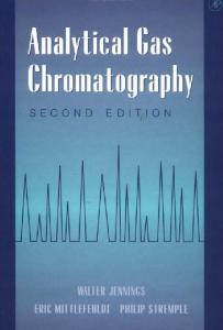
V. THE CHROMATOGRAPHIC PROCESS There are three different approaches to account for the chromatographic process: (i) the stochastic method which uses probabilities to describe the behavior of the molecules of a compound during their elution and is best illustrated by the random walk model (see Chapter 4), (ii) the use of mass-balance equations, the classical method of chemical engineering (see Chapter 5), (iii) the analogy with the Craig machine, which is a cascade of liquid-liquid extractors. Each of these approaches is best suited to a different purpose. The analogy to the Craig machine, although it is somewhat arbitrary, illustrates very well some of the basic concepts of chromatography. The random walk approach permits an excellent, References on p. 33.

8

although somewhat elementary, discussion of the influence of the resistance to mass-transfer on band broadening. The analytical solution of the set of mass-balance equations is not possible in cases which are of real practical interest, so the method can give only the necessary numerical solutions, but does not supply the concepts or images which are required to understand the chromatographic processes. In this section, we give an outline of the Craig machine, in order to illustrate the basic concepts of chromatography (5-11). We do not give a detailed presentation of its theory, however, as it does not really apply to chromatography and does not readily extend to it.

16.

G

1601

I

I

I .8

G

1601

I L

. 8 4.

14.

4.

14.

.2

14.

12.

4.

2.

14.

. 2

1. 1.

13.

3 8

13.

3.

I

3. .3

38

3.

. 2 .2

1601

I G

G

@

13.

-1-H

12. 12.

0 E

.1

'1.

L

12.

3.

L

1.2.

160

G L

I I

1. 1.

160

G L

1.

160

1.

G L

1=

160

G

L

Concentration

Figure 1.2. Schematic of the chromatographic process, considered as an automatic Craig machine. Succession of transfer steps (T) and equilibrium steps (E). G denotes the gas phase, L the stationary phase in a chromatographic column. The lower curve gives the concentration profiles of the two compounds in the Craig machine.

9

Let us divide the column into a series of short reactors, each of unit volume. In each of these reactors, equilibrium of the sample composition between the two phases takes place. The continuous chromatographic process is thus replaced by a succession of a number of two-step processes. In the first step, a volume of gas is transferred from each reactor to the next one; the first reactor is filled with pure carrier gas. In the second step, the reactors are left still, so that equilibrium can be reached in each of the reactors. The sequence is repeated a sufficient number of times to permit elution of all sample components. Although we somewhat arbitrarily introduced a discontinuity in the process, this model correctly identifies the two basic phenomena which underlie chromatography: downstream transfer by the mobile phase and equilibrium between the two phases. If we assume, for example, that we have (cf Figure 1.2) 32 molecules in a sample of a mixture, 16 black ones and 16 white ones, with partition coefficients 0.5 and 0.0 respectively, a very crude assumption indeed, the process takes place as follows (cf Figure 1.2).

First step During the first transfer, the 32 molecules are introduced into the first reactor. During the first equilibrium, the white molecules are not soluble in the liquid stationary phase. They all stay in the gas phase, while the black molecules partition between the two phases, and at equilibrium there are 8 black molecules in the gas phase, 8 in the stationary phase.

Second step Second transfer: The gas phase of the first reactor is transferred to the second one, with the 16 white molecules and the 8 black ones it contains. The other 8 black molecules stay in the stationary phase of the first reactor. The proper volume of pure carrier gas is introduced into this reactor. Second equilibrium: In the first reactor there remain no white molecules. The black ones equilibrate between the two phases, 4 molecules on average are in the gas and 4 in the stationary phase. In the second reactor the 16 white molecules remain in the gas phase, while the 8 black ones partition between the two phases. At equilibrium there are 4 black molecules in the gas phase and 4 in the stationary phase.

Third step Third transfer: The gas phase of the second reactor is transferred to a third one with the 16 white and 4 black molecules it contains, the gas of the first reactor is transferred to the second one with the 4 black molecules it contains, and the first reactor is filled with pure carrier gas. References on p. 33.

10

Third equilibrium: In the first and second reactors there art? no white molecules. They are all in the third one, where they stay in the gas phase since they are not soluble in the liquid phase. The first reactor contains 4 black molecules and at equilibrium there are 2 in each phase. The second reactor is already at equilibrium, with 4 black molecules in each phase. The third reactor also contains 4 molecules, 2 in each phase. Fourth step Fourth transfer: The gas phase of the third reactor is transferred to a fourth one, with the 16 white molecules and the 2 black ones it contains. The gas phase of the second reactor is transferred to the third one, with its 4 black molecules and the gas phase of the first reactor is transferred to the second reactor with the 2 black molecules it contains. The first reactor is filled with pure carrier gas. Fourth equilibrium: Only the fourth reactor contains the non-soluble white molecules. The black molecules are now distributed between the four reactors as follows: 2 in the first one (1 in each phase), 6 in both the second and third reactors (3 in each phase, in each reactor), and 2 in the fourth reactor (1 in each phase). A distribution curve of the two compounds is given in Figure 1.2. The progressive dilution of the retained compounds, their separation when their distribution coefficients are different and the shape of their distribution among the different reactors now appear clearly. Their profile is given by the binomial distribution (5). When the number of reactors is large this distribution tends towards the Gaussian law. Assuming a large number of reactors and a Gaussian distribution, it is possible to relate the number of reactors to the properties of the profile. This number is given by the classical relationship: 2

N = 16(

$)

where t , is the time of the maximum of the distribution and w its base width. By analogy to distillation columns and other systems where continuous separation processes take place, this number has been called the number of equilibrium stages or, more classically, the number of theoretical plates.

VI. DIRECT CHROMATOGRAPHIC DATA

From the data recorded during a chromatographic analysis, five parameters can be measured for each peak, assuming it is well enough resolved from its neighbors (cf Figure 1.3). From these parameters, which vary a great deal when experimental conditions are changed, a number of more fundamental data can be calculated (cf next section).

11

4

I----tR

I I I

I I

I I

1

I

r,

AtR

d

Figure 1.3. Idealized chromatogram showing the ‘air’ peak and the peaks of two compounds. This illustrates the chromatographic symbols.

These five basic experimental data are: 1. The Retention Time, t ,

This is the time between injection of the sample and the appearance at the column’s exit of the maximum concentration of the band of the corresponding compound. 2. The Gas Hold-up Time, t,,,

This is the retention time of an inert compound which is not retained on the column, i.e. a compound not adsorbed or dissolved by the stationary phase. Such a compound is sometimes difficult to find. With most stationary phases air is not or is practically not retained. As air is not detected by some detectors, like the flame ionization detector, methane is often substituted. This is most often satisfactory, but not always. Methane is markedly retained by most adsorbents at room temperature. It is only very weakly soluble in many liquid phases. Other common names given to the gas hold-up are the ‘retention time of a non-retained compound’ and the ‘air retention time’. This last name, which refers to the ancient use of air with a thermal conductivity detector to determine the gas hold-up time, is obsolete and should be avoided.

3. The Peak Width, w

This is usually defined as the length of the segment of the base line defined by its intersection with the two inflection tangents to the peak. The peak width, either at half height or at some other intermediate height, is also used. References on p. 33.

12

4. The Peak Height, I, This is the distance between the base line and the peak maximum.

5. The Peak Area, A This is preferably measured by integration of the signal. The problems associated with the definition of the peak area and the precision and accuracy of its determination are discussed in Chapters 15 and 16. These parameters can be measured using either the lengths measured on the paper chart or, preferably, the units of the parameters measured, time and detector signal (current or voltage). They are rarely used as such but mostly as intermediate for the derivation of the data discussed in the following sections.

VII. DATA CHARACTERIZING THE GAS FLOW The average flow velocity of the gas stream is defined in chromatography as the ratio of the column length, L, to the gas hold-up time, t,:

As the whole pore volume inside the particles of the support or adsorbent is accessible to the air or inert compound, this parameters defines an average calculated over the entire fraction of the column cross-section occupied by the gas phase, whether mobile, around the particles, or stagnant, inside these particles. Thus the average velocity used in chromatography theory is different from the one classically used in chemical engineering. We assume that the permeability of the column is constant all along its length, i.e. that the packing density is constant, which is not a straightforward conclusion, at least for packed columns, considering their packing technology. Then it can be shown (1) that the outlet gas velocity, u,, again averaged over the cross-section available to the gas phase, is given by the following relationship: u, =j X

li =

2 ( ~3 1) li 3( P 2- 1)

(3)

where j is termed the James and Martin pressure correction factor, and P is the ratio of the inlet ( p i )to the outlet ( p o ) column pressures:

p = -Pi Po

(4)

13

These pressures are absolute pressures. Since manometers usually work with reference to atmospheric pressure, accurate measurements require the use of a precision barometer. Usually, P is the absolute inlet pressure in units equal to the local atmospheric pressure at the time of the measurement.

VIM. DATA CHARACTERIZING THE RETENTION OF A COMPOUND

There are two reasons to use data derived from the experimental retention time, rather than t R itself. First, t R varies considerably when the experimental conditions are changed, and it is practical to use data which are constant or more readily reproducible. Secondly, it is possible to derive a relationship between t R and the thermodynamic equilibrium constant. Data which are related to this constant make more sense and are easier to correct for changes in the ambient parameters. 1. The Retention Volume, VR The theory of chromatography shows that the retention time is related to the flow rate of mobile phase across the column. In liquid chromatography the product of the two is constant. Because of the very large compressibility of gases this simple relationship does not hold in gas chromatography, but nevertheless we can define the retention volume as follows:

where F, is the carrier gas flow rate measured at column outlet and at column temperature. If F, is not constant, VRcan be defined by an integral, but this does not result in a practical procedure of measurement. 2. The Dead Volume, V, The definition is the same, but uses the gas hold-up time: V , = t,,, X F,

The dead volume is also called the ‘gas hold-up volume’, the ‘retention volume of a non-retained compound’, which is long and somewhat self contradictory, and ‘the air retention time’, which is obsolete. 3. The True Retention Volume, V/

This is the volume of carrier gas flowing through the column while the compound is dissolved in or adsorbed on the stationary phase. Since all compounds move along the column at a speed 0 when they are interacting with the stationary phase and at a References on p. 33.

14

speed equal to that of the carrier gas when they are in the gas phase, this is the product of the carrier gas flow rate and the difference, tR - t,:

Similarly, t;P is the true retention time. 4. The Corrected Retention Volume,

vR

As explained above, when the carrier gas flow rate increases, the retention volume V, does not stay constant. An increase of the flow rate can be achieved only by increasing the inlet pressure. Thus the same amount of gas at the column inlet occupies a smaller volume, and a larger number of moles of carrier gas is required to elute a compound when the inlet pressure increases. The corrected or limit retention volume is the limit for pi=po of the retention volume (1). It can be shown (see Chapter 2) that:

where j is again the James and Martin factor.

5. The Net Retention Volume, V, This is also called the totally corrected retention volume. This is the true, corrected retention volume:

v,

By convention, VR, V;, and VN are measured at column temperature and at the column outlet pressure. While it is not too difficult to measure the flow rate at the outlet column pressure, a correction is necessary for the temperature. A correction for the water pressure is also required if the soap bubble flowmeter is used. 6. The Specific Retention Volume, Vg

This is the STP net retention volume, divided by the mass of liquid stationary phase in gas-liquid chromatography, or by the total surface area of adsorbent in gas-solid chromatography:

m ,is the mass of liquid phase, T, the column temperature (K) and pn the standard

pressure.

15

Like V i and V,, V, does not depend on the flow rate, but only on the column temperature, the phase system and the compound studied. V,, however, is a physical constant, directly related to the thermodynamic constant of the physico-chemical equilibrium used in the phase system (see Chapter 3). The accurate determination of any one of these parameters is difficult because it requires the measurement of the column flow rate, which can rarely be made with an error less than around 1%. For this reason relative parameters are often preferred in analytical work. Even in thermodynamical studies it is important to realize that the error made on the ratios of retention volumes, and hence on the ratio of the equilibrium constants, is often one order of magnitude smaller than the error made on the absolute value of these constants. Two parameters of this type are often used:

7. The Column Capacity Factor, k’ This is defined directly from the retention times:

k’ is the true retention time measured with the gas hold-up time as a unit. 8. The Frontal Ratio, R This is the ratio of the ‘air’ to the solute retention times:

Combining equations 11 and 12 gives: 1-R k ’ = - and R

1 R=1+k’

The theory of chromatography defines R as the fraction of the number of molecules in the mobile phase at a given time; of course 1- R is the fractional number of molecules in the stationary phase. As the molecules in the gas phase move at a speed equal to u and those in the stationary phase at a speed 0, the average speed of the molecules is Ru, hence equation 12. A more rigorous discussion is given in the literature (7). Thus, k’ is the ratio of the number of molecules present in the two phases and, accordingly, is proportional to the apparent thermodynamic constant of equilibrium. References on p. 33.

16

IX. DATA CHARACIXRIZING THE COLUMN EFFICIENCY

The larger the band width the more difficult it is to separate the components of a mixture, since there is less room to place them on the chromatogram. The analyst will thus strive to produce narrow, well-resolved peaks. Another advantage of narrow bands is that the maximum concentration of the eluate is large, which makes detection more sensitive with a given detector, a very useful feature in trace analysis.

1. The Standard Deviation, u In many cases, in analytical applications of chromatography, the peak profile can be assumed to be Gaussian. Accordingly, the chromatographic trace is described by the following equation:

The signal is equal to its maximum value, y, for t = t,, which is the definition of the retention time. Sigma is the standard deviation of the Gaussian curve. Its square, u2, is the variance of the Gaussian curve. These two parameters, the standard deviation and the variance, are used in the study of chromatographic band broadening. It must be emphasized that, while the standard deviation is defined only for a Gaussian profile, the variance can be defined for any distribution, and becomes equal to the square of u in the case of a Gaussian profile. The properties of the Gaussian curve have as a result that the inflection tangents define on the base line a segment of length w: w=4u

(15)

which relates the peak width to the standard deviation. The width of the Gaussian curve at each fractional height is related to the standard deviation. Equation 1 4 can be rearranged to give:

or :

where w, stands for the width at the fraction x of the peak height.

2. The Different Standard Deviations The standard deviation can be measured in different units at the column outlet, or at any place in the column. When the band resides inside the column, it is

17

distributed along a certain fraction of the column length, with a Gaussian profile. The standard deviation is then measured in length units. When the peak is recorded on a chromatogram, the standard deviation can be measured on this trace in time units. The relationship between these two values is: (11 = RUU,

(18)

We note in passing that, if the band profile is Gaussian inside the column, at a certain time (i.e., the plot of solute concentration versus abscissa along the column), the elution profile (i.e., the plot of solute concentration versus time at column exit) cannot be Gaussian. The sources of band broadening, such as diffusion or resistance to mass transfer, continue to act on the part of the profile which is not yet eluted, resulting in an unsymmetrical elution profile. We may consider this elution profile to be analogous to a Gaussian profile, but with a standard deviation which increases slowly with increasing time. The effect is small, however, and may be neglected. Finally, at column outlet, the band occupies a volume of mobile phase equal to: 401F, v = 4 a,,= 4 a, F, = Ru It is important to note that when they are used, uI is determined just before column exit, inside the column, while a,, is determined just after the column exit, in the gas stream. This explains the factor Ru in equation 19. The width of the peak profile is important, but mainly in comparison to the retention time, which gives the time scale of the chromatogram. For this reason several dimensionless parameters have been defined (see f, N , H , below). 3. Properties of the Variance

There are several properties of the variance which are discussed in greater detail in Chapters 2 and 13, but which are worth mentioning here, since they explain the importance attached to these parameters (14). Let us assume that we have a large number of molecules which can move in only one direction (i.e. the column axis; radial distribution is assumed here to be homogeneous). Their movements take place by random leaps and bounces of length 1. When each molecule has had the opportunity to achieve a large number, n, of leaps, the molecular distribution along the column axis will be Gaussian, with a variance given by: a: = n

x 1’

(20)

This is the equation of the unidimensional random walk (14). It can be used to calculate the contribution to the band variance of the various phenomena which tend to spread the distribution of the molecules of a compound (molecular diffusion, unevenness of the pattern of flow velocities, resistance to mass transfer, cf Chapter 4). References on p. 33.

18

The power and simplicity of this model result from the fact that if several independent random phenomena contribute to the band broadening, then the resulting variance is the sum of the variances of each independent phenomenon:

All that is necessary is a complete census of the various contributions to band broadening and the calculation of each individual variance. 4. The Relative Peak Width, f

This is the ratio:

5. The Number of Theoretical Plates of the Column, N

This number is given by the relationship:

):(

N = 16( $ ) 2 =

2

= 16f2

From equation 17, we can also write: 2

N = 5.54( 5) w0.5

which permits the derivation of the plate number from the width of the peak at half-height, often measured with more accuracy than the base line width (23). This parameter has been defined previously (cf Section V), using the plate theory. It is redefined here, independently of any theory, with the assumption of a Gaussian peak profile. This definition is not valid for an unsymmetrical peak, although the plate number is sometimes measured for such peaks, leading to data for which it is impossible to account and which are often controversial (15).

6. The Number of Effective Theoretical Plates, N , The definition is the same as for the theoretical plate number, but this time the true retention time, t;, is used:

$)

2

N-, = 16(

19

7. The Height Equivalent to a Theoretical Plate, HETP or H If the column of length L has a number of theoretical plates N,we can consider that, on the average, each plate has a height H such that:

-= L H

N

This is somewhat artificial, because these plates are not bound by physical limits in the column, they are merely theoretical, and defined artificially, because of the analogy with the Craig machine (cf Section V and equation 1)and because of a still more superficial analogy with distillation columns. The HETP is quite similar to the transfer unit length of chemical engineering. In fact it is possible to redefine the HETP in a more meaningful and useful way, by considering the local plate height, H(z), where z is the abscissa along the column (7). H ( z ) is defined as the proportionality coefficient between the distance dz and the differential increase in band width when the peak moves forward a distance dz from the abscissa z to the abscissa z dz:

+

daf=H(z)dz

(27)

If the local plate height were constant along the column (dH(z)/dz = 0), integration of equation 25 would give a result identical to equation 24, but it is always possible to define an average plate height:

JO

and then:

This problem is discussed in more detail in Chapter 4. The importance of the HETP results from the fact that it can be considered as the length of column necessary to achieve equilibrium between the two phases. Contrary to what happens in the theory of the Craig machine, however, the HETP does depend on the experimental conditions (cf Chapter 4). It should be emphasized here that if we apply the definition of equation 27 to the Craig machine, the value obtained for the HETP is not equal to 1 (plate), but to 1 - R (fraction of molecules in the stationary phase at equilibrium); consequently, the plate number is not equal to the number of reactors in the machine (25). This illustrates the inconsistency between the Craig machine model and the classical model of chromatography. As with most analogies, the Craig machine model should be used merely for its pedagogic value, not as a predictive tool. References o n p. 33.

20

AS=

BC AB

Figure 1.4. Definition of the band asymmetry. The asymmetry is usually defined as As=BC/AB, sometimes as As = B’C’/A’B’.

Time in seconds; concentration in arbitrary units.

8. The Band Asymmetry, As Peaks recorded in gas chromatography are not always Gaussian. In a number of cases the bands are quite unsymmetrical. There are several explanations for that fact, which are discussed in Chapter 4. It may then be useful to characterize the asymmetry, to study the influence of changes in experimental conditions and find trends and/or correlations. The most simple and useful parameter is the ratio of the two segments of the base line defined by its intersection with the vertical from the peak maximum and the two inflection tangents (A’B’/B’C’, Figure 1.4). The ratio of the two similar segments defined on the parallel to the base line at the peak half-width by the profile itself and by the vertical from the peak maximum is easier to measure, but usually much closer to unity (AB/BC, Figure 1.4).

X. DATA CHARACTERIZING THE SEPARATION OF TWO COMPOUNDS

Parameters relative to the characteristics of both peaks are used. They relate to the retention of and to the separation between the two peaks. These two peaks are referred to as #1 and # 2 in the following discussion. The most important parameters are the relative retention of two compounds, the retention index, the resolution between two compounds and the effective peak number or peak capacity of a column.

21

1. The Relative Retention, a This is the ratio:

It is defined and usually calculated so as to be larger than unity. In some cases, when a large number of compounds are referred to the same standard compound, or when a vanes with temperature, values smaller than unity may be considered. a depends on the stationary phase and is a function of the temperature. As a first approximation, it does not depend on the flow rate, the inlet pressure or the nature of the carrier gas (see Chapter 3). It is easier to calculate than the absolute retention data (specific retention volume or partition coefficient) and more accurate. Accordingly, it is frequently used. 2. The Retention Index, Z This is the most important retention parameter in practice, at least in the analysis of organic compounds (16). The retention index is related to the relative retention a [ X / n P Z ]of a compound, X , to the normal alkane eluted immediately before it, under the same conditions. z is the number of carbon atoms of this n-alkane. The retention index is: I ( X ) = 100

log( a X/HP,) log( a nP, + 1 / n P 2 )

+ 100 z

a nP, + l / n P , is the relative retention of two successive n-alkanes. It is practically constant when z exceeds 3 or 4 (see Chapter 11). The retention index system is now widely used, because of a combination of theoretical and practical advantages: - the system uses a reference scale based on the n-alkanes, which are well defined compounds, readily available, easy to elute in most cases, and covering a wide range of volatility, so it is almost always easy to find a pair of n-alkanes that are eluted just before and just after the studied compound. - a varies very rapidly with the temperature. Usually it is similar to an exponential function. Accordingly, I( X ) is an homographic function of temperature, but in a reasonable range, due to the mode of selection of the reference compounds, I ( X ) varies slowly enough and the dependence can be considered to a good approximation to be linear. The values dZ/dT are small for hydrocarbons, larger for compounds with polar groups, they can be tabulated to permit interpolation and supply some information for qualitative analysis. - although this does not readily appear from the definition, the system in fact uses a linear scale of free energies of dissolution in the fixed liquid phase or References on p. 33.

22

adsorption on the stationary phase. Because of this thermodynamic background, the retention index system enjoys some fundamental properties. For example, linear free energy relationships can be used to calculate the retention index of compounds which are not available, or for assisting in the identification of unknowns. A considerable amount of the literature deals with this problem (see Chapter 11). There are cases where the use of n-alkanes as reference compounds does not give satisfactory results, especially when the compounds studied are best resolved on strongly polar phases. Then n-alkanes are weakly soluble and mainly retained by adsorption at the liquid-gas interface. Their retention volume is not proportional to the amount of liquid phase, the retention index depends on the phase ratio, and the column loadability for n-alkanes may be extremely small. Then it is possible to replace the n-alkanes as the reference series by another homologous series such as the n-alkanols, n-alkyl phenols, fatty acid methyl esters, etc.

3. The Resolution, R,,2 The resolution between two peaks is defined by the equation:

It is the ratio of the difference between the two retention times to the average base line width of the two peaks. If the resolution is unity the tail inflection tangent

L

Figure 1.5. Idealized chromatograms showing two peaks with the same height and different values of their resolution. 1: R = 0.50; 2 : R = 0.75; 3: R = 1.00; 4: R =1.25; 5: R = 1.50; 6: R = 1.75. When the resolution is unity, the two inflexion tangents intersect on the base line. There is no return to base line for resolution smaller than ca 2.0. Time in seconds; concentration in arbitrary units.

23

of the first peak intersects the front inflection tangent of the second peak on the base line (cf Figure 1.5). There is no return of the recorder trace to the base line, but if the two peaks have equal size the valley trough is 27%of the common peak height. Interference is thus still too important to permit a good quantitative analysis. With a resolution around 1, difficult decisions must be made regarding peak area allocation between the two compounds. This cannot be done accurately for peaks of

0.8C ._ 0 0.7-

+

> 0.6C

al

2

0.5-

0

V

0.4 Q3 0.2

3 50

370

390

410

430

450

4 70

490

430

450

470

490

Time

0.260.240.22-

c

0.2-

0 .-+

0.18-

L

$

5

0.160.140.120.1

-

3 50

Figure 1.6

370

390

410

Tme

(Conhued on p . 24) References on p. 33.

24

The

-

1.0

0.9-

0.80.70 .u o .0.6-

u C

s

0.5-

0 a4-

0.3-

0.2-

-

0.1

o.o+ 350

370

390

410

430

450

470

490

Time

Figure 1.6. Influence of the relative peak height on the profile of a doublet with constant resolution. (A) R =1.00.Relative peak height: 1: 1.0; 2: 0.30;3: 0.10;4:0.03.

(B) R =1.50. Relative peak height: 1: 0.30; 2: 0.10;3: 0.030;4:0.010. (C)R =1.50. Relative peak height: 1: 1/10; 2: 1/100; 3: 1/1,OOO; 4: 1/1O,OOO; 5: l/lOo.OOO. (D)R = 2.00. Relative peak height: 1: 1/10; 2: 1/100; 3: 1/1,OOO; 4: 1/1O,OOO; 5: 1/100,OOO; 6: 1 /l,OOo,OOO. Time in seconds; concentration in arbitrary units.

25

unequal heights, when the resolution is less than 1.5 to 2, depending on the height ratio (see Figure 1.6). A good quantitative analysis requires a resolution of cu 1.5. When the resolution decreases below 1.0 the interference between the two peaks becomes stronger and stronger, and the valley disappears at R = 0.5. When the ratio of the two peak heights becomes very different from unity, those requirements change and become more drastic, especially for a proper quantification of the smaller peak (cf Figure 1.6). When the resolution between two compounds is great it is rarely measured, except perhaps for the derivation of the peak capacity. When it is small, it is possible to derive an important relationship between the resolution, the relative retention of the two compounds, the column capacity factor for one of them and the column efficiency, by making a simple approximation. Since the resolution is small, we can assume that the column efficiency is identical for the two compounds, hence:

Combination with equations 7, 11, 23 and 32, and assuming that tR,l and t R z are close enough and that tR,l+ t R , 2 is equivalent to 2 f R . 2 , give:

or :

fi x-xa-1

R=-

4

a

k‘ 1+k‘

(35)

where k’ stands for k ; , the capacity factor for the second compound (17). This relationship is very important because it permits the derivation of the plate number necessary to achieve the separation of a given pair of compounds, knowing their relative retention and the capacity factor of the column for the second one. It shows that no matter how efficient the column is, there is no separation if there is no resolution. In difficult cases, k’ should be optimized to ca 3-4, for rather large resolution power and a still reasonable analysis time. It has been shown that the minimum analysis time is achieved in conditions where k’ is around 1.5-2 for open tubular columns and 3 for conventional packed columns (24). Equation 35 also sets a minimum limit to the relative retention of two compounds which can be separated with a column of given efficiency. In t h s equation, a! and k’ for a given pair of compounds depend only on the phase system selected and to some degree on the temperature, but not on the column, while N depends essentially on the column length and the packing material used. The resolution of a given pair of compounds is thus proportional to the square root of the length of the column used. References on p. 33.

26

4. The Separation Factor, I:

This parameter was introduced by Giddings (7), but it has rarely been used. The definition is similar to that of the reso1ution;and it is easier to use when the plate numbers for the two compounds are markedly different. This is not a situation of practical importance, however.

When the two peaks are close and the column plate number is the same for both, F is equal to the square of the resolution. It is easy to show that: F-

(DK)’L 16H(p

+ K)’

(37)

where DK is the difference between the partition coefficients of the two compounds, K the average ( K , + K , ) / 2 , and B is the column phase ratio, V,/V;, the ratio of the volumes of gas and liquid phases contained in the column. This direct relationship between the separation factor and the thermodynamic constants of the phase system makes it interesting for theoretical studies. 5. The Effective Peak Number, EPN

This parameter which characterizes the separation power of a column in a particular range of retention is also called the separation number, TZ. It is defined as the maximum number of peaks of equal heights one can place between the peaks of two reference compounds, assuming a resolution of 1.0 between each one of these peaks (18). Obviously it is most convenient to select as reference compounds two successive n-alkanes or two successive homologs. If, as a first approximation, it is assumed that the base line width of these peaks varies linearly, we may write: EPN(1,2) =TZ(1,2) = R1,’- 1

(38)

It is important to realize that the separation number can change markedly from one pair of compounds to the next one, thus the linear approximation made in the derivation has only a coarse validity. This is especially true for open tubular columns. It is therefore necessary to indicate which pair has been used for the measurement. Furthermore the separation number also depends strongly on the column temperature, increasing rapidly with decreasing temperature, which explains why too many authors use unrealistically low temperatures to rate their columns. Although this parameter is useful to compare columns in strictly defined experimental conditions, it must be used very carefully, otherwise it may easily turn out to be a ‘rubber ruler’ (19).

21

XI. DATA CHARACTERIZING THE AMOUNT OF A COMPOUND There are two parameters which can be used for this purpose, the peak height and the peak area. I

1. The Peak Height

The peak height is the maximum deviation of the detector signal from the base line during the elution of the corresponding compound. This requires the interpolation of the background signal during this elution. The determination of the peak height is difficult if there is a significant base line drift during the analysis, as such a drift is usually not linear and the estimate of the value of the background signal at the time of the peak maximum may be inaccurate. In the case of closely eluting compounds it may become impossible to form any estimate of the background signal between the two peaks. Extrapolation is then necessary. If the two peaks interfere, each peak height may be biased by a contribution from the other compound. Such a contribution is 1%for two equal sized compounds distant by 3 standard deviations (resolution = 0.75). Thus, peak height measurement may be more accurate than peak area in the quantitative analysis of compounds which are poorly resolved, providing that the operating conditions, and especially the injection, remain strictly constant. The importance of this requirement must be stressed.

2. The Peak Area The peak area is the area under the signal. In principle the integration should be carried out from the injection time to infinity. Fortunately, the signal returns rapidly to zero after the peak maximum is eluted, and integration does not need to be performed over a range exceeding - 3 to 3 standard deviations. The peak area is proportional to the sample size as long as (i) all the sample is eluted, without decomposition, reaction or irreversible adsorption, and (ii) the detector is linear. This is true, even if the column is overloaded or for any other reason gives unsymmetrical peaks. This is an advantage over the peak height, which does not vary linearly with sample size under these conditions. If the detector used is linear, that is if the detector response is always proportional to the concentration of component in the stream of carrier gas, the peak size is proportional to the amount of compound contained in the injected sample. If the peak profile were Gaussian, the peak height as well as the peak area would be proportional to the amount of compound. There are, however, reasons other than non-linear detector behavior for the observation of peaks whose height is not proportional to the sample size. Furthermore, the fluctuations of experimental parameters do not affect peak height and peak area in the same way. The choice between height and area to base quantitative analysis is discussed in detail in Chapter 16, together with the sources of errors on both measurements.

+

References on p. 33.

28

The peak profile is often assumed to be Gaussian. Within the limits of validity of this assumption, the concentration at peak maximum is given by the following relationship:

rnfi

C,= -

(39)

VR&

The peak height depends on the plate number of the column and the retention volume of the analyte. This explains why, in trace analysis, better results are obtained under conditions where the retention time is relatively small, and the efficiency important. Dilution proceeds constantly during the chromatographic process, at a speed which is at least equal to that of pure molecular diffusion along the column axis. The shorter the analysis time, the lower the additional dilution of sample in the mobile phase. This is an important factor, because even'if the peak area is often the parameter measured to carry out quantitative analysis, the detection limit depends essentially on the peak height, and only a little on its width. Finally, it should be emphasized here that the peak area is the integral of the detector signal with respect to time, while the mass of a compound is the integral of its concentration with respect to the volume of carrier gas. Fluctuations of mobile phase flow rate and pressure (i.e. density) in the detector will introduce errors in quantitative analysis for this reason.

XII. DATA CHARACTERIZING THE COLUMN Although these data are not determined from the chromatogram, they are often necessary to evaluate the chromatographic data.

1. The Column Length, L 2. The Column Inner Diameter (abbreviated i.d.), d , These two dimensions are often supplied by the manufacturer. They may be difficult to measure, especially on a coiled prepared column. When packed columns are properly cut, d , may be measured by determining the size of the largest drill which can fit inside the column. For empty packed and open tubular columns, the inner diameter can be determined by weighing the column both empty and filled with water, a solvent of known density or mercury (which is better for open tubular columns (OTC)). 3. The Particle Size, d ,

For packed columns (PC), it is determined by sieving. The mesh sizes of sieves are normalized (cf Table 1.1). It can also be derived from measurement of the column permeability.

29

TABLE 1.1 Relationship between Normalized Sieve Mesh Size and the Average Size of the Particles which pass through them. Opening (mm) 0.080 0.083 0.100 0.104 0.124 0.125 0.147 0.149 0.160 0.175 0.177 0.200 0.208 0.210 0.246 0.250 0.295 0.297 0.315 0.351 0.400 0.417 0.420 0.500

USA ASTM E 11 39

USA WS Tyler Mesh

French AFNOR N F X MM

German DIN 4188

Japanese JIS Z 8801'

20 170

170

170

88

145

105

120

125

100

149

80

177

65

210

55

250

48

297

42

350

36 32

420 500

21 140

150 115

120

22

100 24 80 80 24 65 70 60 25

60

48 50 26 45

42 27 35

40 35

28

An accurate knowledge of either the column diameter (OTC) or of the average particle size (PC) is required for a proper assessment of the results of the determination of the column efficiency at various flow velocities of the carrier gas.

4. The Coating Ratio This is the weight of liquid phase with which a certain weight of the support is coated (w/w, W).

5. The Gas Hold-up, V, This is the retention volume of an inert compound. This is also the total volume of the column available to the mobile phase.

6. The Phase Ratio, /3 This is the ratio of the volume of stationary phase to the volume occupied by the mobile phase. References on p. 33.

30

XIII. PRACTICAL MEASUREMENTS In practice, there are three different methods to derive raw data from a chromatogram. The trace of a potentiometric recorder is measured with a ruler, the print-out of an electronic integrator is read, or data are acquired with a computer and processed automatically. The choice between these methods depends on the money available for investment, but also on the nature of the problem to be solved and it is important to understand the basic problem specific to each one of these three methods. The problems of quantitation are discussed extensively in the following chapters, so only a brief survey is supplied here. Direct measurements on the recorder trace are easy but tedious and time consuming. The precision is limited to a few percent, but fundamental errors are rare. A very simple method of determination of retention distances is illustrated on Figure 1.7 (20). The drawing of proportional triangles permits the rapid and precise (a few percent) determination of relative retention times. A straight line is drawn between the point on the origin of the signal scale at the time of the ‘air’ peak and the point on the signal full scale deflection at the retention time of the reference compound. Parallel lines are then drawn as shown on Figure 1.6. The relative retention times increase each time by one unit. The lines perpendicular to the base line through the peak maxima are drawn until their intersection with the line AC‘ or one of its parallels. The relative retention times are read on the vertical scale. Peak heights are also easy to measure. Proper calibration permits their use in quantitative analysis. Although the precision of such measurements is basically limited, it is not certain that the improvement in precision which can be achieved by turning to manual integration of the peaks justifies the considerable increase in the amount of work required. The various methods of manual integration have been studied in detail by Harris, Habgood and Ball (21). This problem is discussed further in Chapters 15 and 16. Electronic integrators work on-line, cannot keep the chromatogram in memory nor make decision based on later events, and operate according to decision made by their designers, which the analyst cannot change, which may be bad, and of which he is often not aware, which is much worse. For example the retention time is not the time when the derivative of the detector signal becomes zero, after a peak has been detected, but the time when this derivative becomes negative, and equal to the threshold indicating the end of a peak. The result is a systematic delay, which increases with increasing band width, and may be significant, especially in isothermal analysis, when retention times are most prone to be measured, because the band width increases regularly, with increasing retention, and so does the delay. Similarly, as shown by Bauman, there is a systematic error due to the influence of the base line drift correction on the measurement of the peak area (22). In principle the analyst who uses a computer can check the programs and adapt them to his problems. Unfortunately, this is often quite impractical, because the programs which are purchased are protected or at least often supplied in compiled language. Even a nice looking print-out of somebody else’s program is not easy to

31

23 min

Y

,I

0

0

A

Figure 1.7. Example of a simple chromatogram. Graphic determination of the relative retention times. Standard: toluene. Column: i.d. 4 mm, length: 4.0 m, packed with 15% triscyanoethoxypropae on Chromosorb P, 60/80 mesh, followed by 0.60 m of 15% Carbowax 20M on the same support. Temperature: column 100°C, injector and detector: 15OoC. Camer gas: Nitrogen, 3.0 l/h. Flame ionization detector: 2.0 I/h hydrogen and 15 l/h air. See list of compounds and retention times in Table 1.2.

TABLE 1.2 Relative Retention Times of the Compounds on the Chromatogram Figure 1.7 No.

Compounds

r;((x)/r;((toluene)

1 2 3

Methylene chloride Ethyl acetate Ethanol Methyl ethyl ketone Toluene Butyl acetate m-Xylene

0.23 0.39 0.47 0.14 1.00 1.47 2.54

4

5 6 7

NB. The standard compound, here toluene, should be chosen so that the relative retention times are between 0.1 and 10. Otherwise the precision of the measurements becomes poor.

understand and still more complex to modify. Strange results should be expected at the first attempt. Special attention should be paid to the methods of peak area allocation used in References on p. 33.

32

the case of incompletely resolved bands. Very large errors can be introduced by relying too heavily on the solutions programmed by computer scientists who have a limited understanding of chromatography and are only trying to help by interpolating base line or solvent peak profiles and using various algorithms of curve fitting to allocate the area measured. But in more cases than is presently realized by many, our experience is that these procedures are not legitimate, because the chromatographic process in such cases is not linear, as it is assumed in all those treatments. The actual solution is almost always in the achievement of a better resolution and a more accurate calibration. The problems encountered when using each one of these different approaches to the quantitation of chromatographic analysis are discussed in detail in the following chapters.

GLOSSARY OF TERMS

chi

Maximum concentration of a compound in the elution band. Equation 39 Difference between the partition coefficients of two compounds. Equation 37 Column diameter (i.d.) dc Average particle diameter dP EPN Effective peak number or peak capacity. Equation 38 F Separation factor. Equation 36 Carrier gas flow rate. Equation 5 F, Relative peak width. Equation 22 H Height equivalent to a theoretical plate. Equation 26 H ( z ) Local value of H. Equation 27 I Retention index. Equation 31 Correction factor for gas compressibility. Equation 3 j K Partition coefficient of a compound between the two phases. Equation 37 k' Column capacity factor. Equation 11 L Column length. Equation 2 I Average length of a step in the random walk model. Equation 20 Mass of liquid phase in the column. Equation 10 m, N Plate number. Equation 1 4, Effective plate number. Equation 25 n Number of steps in the random walk model. Equation 20 P Inlet to outlet pressure ratio. Equation 3 Inlet pressure. Equation 4 Pi Standard pressure. Equation 10 P" Outlet pressure. Equation 4 PO R Frontal ratio. Equation 12 Resolution between the peaks of two compounds. Equation 32 4 2 Column temperature. Equation 10 T, TZ Separation number. Equation 38 DK

L

33

Time. Equation 14 Gas hold-up time, or retention time of an inert compound. Equation 2 Retention time. Equation 1 True retention time of a retained compound. Equation 7 Carrier gas velocity. Equation 18 Average carrier gas velocity. Equation 2 Outlet carrier gas velocity. Equation 3 Inlet carrier gas velocity. Specific retention volume. Equation 10 Volume of liquid phase contained in the column. Equation 37 Dead volume. Equation 6 Net retention volume. Equation 9 Retention volume. Equation 5 True retention volume of a retained compound. Equation 7 Corrected retention volume. Equation 8 Peak width at base line. Equation 1 Peak width at half height. Equation 24 Peak width at the fraction x of its height. Equation 17 Fraction of the peak height. Equation 17 Detector signal. Equation 14 Peak maximum or maximum of the detector signal. Equation 14 Abscissa along the column. Equation 27 Relative retention of two compounds. Equation 30 Phase ratio of the column. Equation 37 Standard deviation of the peak, if Gaussian. Equation 14 Standard deviation of the contribution of a phenomenon to the band width. Equation 21 Standard deviation in length unit. Equation 18 Standard deviation in time unit. Equation 18 Standard deviation in volume unit. Equation 19

LITERATLJRE CITED (1) A.T. James and A.J.P. Martin, Biochemistry Journal, 50. 679 (1952). (2) All journals dedicated to chromatography and most general analytical chemistry journals. Journals dedicated to other techniques publish papers on ‘hyphenated’ techniques involving GC, while journals devoted to analytical chemistry problems publish reports on applications of GC. (3) Gas Chromatography Abstracts (1957-1969), Gas and Liquid Chromatography Abstracfs (1970-1985). Chromatography Abstracts (since 1986), now published semimonthly by Elsevier Applied Science Publishers, Barking, Essex, UK. (4) CA Selects: Gas Chromatography, published semiweekly by Chemical Abstracts Service, Columbus, OH. ( 5 ) A.I.M. Keulemans, Gas Chromatography, Reinhold, New York, NY, 1959. (6) R.L. Pecsok, Principles and Practice of Gas Chromatography, Wiley, New York, NY, 1959. (7) J.C. Giddings, Dynamics of Chromatography, M. Dekker, New York, NY, 1965. (8) L.S. Ettre and A. Zlatkis, The Practice of Gas Chromatography, Interscience, New York, NY, 1967.

34

(9) H.M. McNair and E.J. Bonelli, Basic Gas Chromatography, Varian, Walnut Creek, CA, 1969. (10) A.B. Littlewood, Gas Chromatography, Principles, Techniques and Applications, Academic Press, New York, NY, 2nd ed. 1970. (11) G. Guiochon and C. Pommier, Gas Chromatography in Inorganics and Organometallics, Ann Arbor Science Publishers, AM Arbor, MI, 1973. (12) D.J. David, Gas Chromatographic Detectors, Wiley, New York, NY. 1974. (13) Practical Manual of Gas Chromatography, J. Tranchant Ed., Elsevier, Amsterdam, 1969. (14) J.C. Giddings, in Chromarography, E. Heftmann Ed., Van Nostrand Reinhold, New York, NY, 1975,p. 27. (15) B. Bidlingmeyer and F.V. Warren, Ana!ytical Chemistry, 56, 1583A (1985). (16) E. sz Kovats, in Aduances in Chromatography,J.C. Giddings and R.A. Keller Eds., M.Dekker, New York, NY, I, 1965,p. 229. (17) J.H. Purnell, Journal of the Chemical Society, 1268 (1960). (18) R.A. Hurrell and S.G. Perry, Nature, 196, 571 (1962). (19) J. Krupcik, J. Garaj, J.M. Schmitter and G. Guiochon, Chromarographia, 14, 501 (1981). (20) C.L.A. Harbourn, BP Research Center, Sunbury on Thames, UK, 1957,private communication. (21) D.L. Ball, W.E. Harris and H.W. Habgood, Journal of Gas Chromotography, 5, 613 (1967). (22) F. Bauman and F. Tao, Journal of Gas Chromatography, 5, 621 (1967). (23)G. Guiochon and J. Schudel, in preparation. (24) E. Grushka and G. Guiochon, Journal of Chromatographic Science, 10, 649 (1972).

35

CHAPTER 2

FUNDAMENTALS OF THE CHROMATOGRAPHIC PROCESS Flow of Gases through Chromatographic Columns TABLE OF CONTENTS Introduction . . . . . . . . . . . . . . . . . . . . . . . . . . . . . . . . . . . . . . . . . . . . . . . . . . . . . . . . . . . . I. Outlet Gas Velocity 11. Column Permeabilit Ill. Gas Viscosity . . . . 1V. Velocity Profile . . . Average Velocity and Gas Hold-up Time . . V. VI. On the Use of Very Long Columns . . . . . . . . . . . . . . . . . . . . . . . . . . . . . . . . . . . . . . . . VII. Case of Open Tubular Columns . . . . . . . . . . . . . . . . . . . . . . . . . . . . . . . . . . . . . . . . . . VIII. Measurement of the Carrier Gas Velocity . . . . . . . . . . . . . . . . . . . . . . . . . . . . . . . . . . . . IX. Determination of the Column Gas Volume . . . . . . . . . . . . . . . . . . . . . . . . . . . . . . . . . . . X. Case of a Non-ideal Carrier Gas XI. Flow Rate through Two Columns ................................... XU. Variation of Flow Rate du .......... XIII. Flow Rate Programming. ......................................... GlossaryofTerms . . . . . . . . . . . . . . . . . . . . . . . . . . . . . . . . . . . . . . . . . . . . . . . . . . . . . . . . Literature Cited . . . . . . . . . . . . . . . . . . . . . . . . . . . . . .

35

44 45

47 48 48 49

51 52 53 54

INTRODUCTION The injection of a certain amount of a pure compound into a chromatographic column is followed, after a certain time, by the elution of a peak, band or zone. (These names are given to the concentration profile of the compound as eluted from the column and recorded by the chromatograph.) The injection of a mixture results in the elution of a number of bands, ideally one for each component of the sample. In linear chromatography, i.e. in practice, in analytical applications of gas chromatography, the set of peaks recorded is the sum of the peaks which would be obtained as a result of the successive injections of the pure components in amounts equal to what exists in the injected sample of the analyzed mixture. In most cases, the time of the peak maximum and some parameter characterizing the band width are of major interest, while the profile itself is not studied in detail. The retention time depends on two independent series of parameters: those accounting for the flow velocity profile along the column, and those describing the thermodynamics of equilibrium between the mobile and the stationary phase (cf. Chapter 3). In addition the band width of peaks corresponding to small amounts of solute depends on the kinetics of mass transfer of the sample molecules in the mobile and the stationary phases and between these two phases (cf. Chapter 4). The band width and the profile of the elution bands of large samples are also functions of the equilibrium thermodynamics (isotherms: cf. Chapter 5). These relationships are important to a discussion of a good understanding of the References on p. 54.

36

basic phenomena observed in chromatography. They are presented in this chapter, as well as in the three following ones, but without much detail on the physico-chemical background involved, since it is not the aim of this book to present a detailed discussion of the theory of gas chromatography. The migration of a solute zone through a chromatographic column is made under the influence of the gas flow, which at the same time plays a determining role in band broadening (cf. Chapter 4). On the average the molecules of all compounds spend the same amount of time in the mobile phase. During that time they move along the column at the same speed as the carrier gas. During the time they spend in the stationary phase they do not move at all; their velocity is zero. Accordingly, the gas hold-up, or retention time of an inert compound, is an important parameter to consider. It serves as a convenient unit for the measurement of retention times (cf. definition of k ' in Chapter 1 and next chapter). The carrier gas flow can be characterized by either the volume flow rate or the linear flow velocity. For a given velocity the flow rate will be greater the larger the column diameter. Since the flow velocity is the important parameter from the standpoint of the chromatographic process, this is the one which should be considered. For the sake of precision it should be measured directly, not derived from the flow rate measurement, since the determination of the exact column diameter is often difficult, if not impossible, especially in the case of capillary columns. The mobile phase flows across the column. Whether this column is packed or is an open tube, it offers some resistance to the gas flow. This resistance is overcome by delivering the mobile fluid to the column under pressure. But gases are compressible: accordingly there is a pressure and a velocity profile along the column: i.e. the local velocity is a function of the position along the column. Of special interest are the outlet velocity and the average velocity, which is related to the retention time. We shall discuss these parameters in turn, then indicate how they are related and how they can be measured. The distribution of the true local gas velocity is extremely complex in a packed column, where the channels open to the gas flow are constantly changing shape and dimensions (1). Furthermore there is a distinction to be made between the stagnant part of the mobile phase which resides inside the particles of porous support used to disperse the stationary liquid phase and the really mobile gas phase which flows around these particles. It can be shown that the velocity inside the pores of the particles is negligible, while the gas flow surrounding the particles, although laminar, makes a large number of stable eddies, located between these particles at the places where the cross section of the channels available to the gas phase changes abruptly (1).With open tubular columns the flow structure is somewhat simpler. To a first approximation the column cross-section is constant, the flow stream lines are parallel to the column wall and the local velocity in a column cross-section is given by a parabolic relationship, maximum at the column center, zero at the wall (2). However, capillary columns are always coiled and the resulting centrifugal force creates a secondary radial flow which, if important, can significantly alter the distribution of flow velocities.

31

I. OUTLET GAS VELOCITY The gas flow velocity through a packed column is laminar (1,3). At moderate values of the gas velocity, normally used in practical applications of gas chromatography, the local velocity is related to the column characteristics by the Darcy law:

where: u is the local velocity, or velocity at point x, k is the column permeability, independent of the nature of the fluid used (gas, super critical fluid, liquid), is the carrier gas viscosity, dp/dx is the local pressure gradient. The minus sign indicates that the gas flows in the direction opposite to the pressure gradient, i.e. from high to low pressures. Equation 1 can be integrated between the inlet and the outlet of the column, whch supplies the value of the outlet velocity. If we assume that the carrier gas is ideal, we have the classical equation: PU = P O U O

where u, is the outlet gas velocity, while p and po are the local and the outlet pressure, respectively. The situation of a non-ideal carrier gas has been discussed by Martire and Locke (4). It applies to CO, used as a carrier gas at inlet pressures larger than cu 5 atm. Elimination of u between equations 1 and 2 gives a differential equation, easy to integrate into:

kP0

u o = - ( P 2 - 1)

2vL

(3)

where P stands for the inlet to outlet pressure ratio ( P= pi/po). In practice the outlet pressure is kept constant, equal to the atmospheric pressure. Then the outlet velocity increases much faster than the inlet pressure. This is due to the decompression of the carrier gas. It should be noted in passing that the Darcy law is empirical in nature. When the flow velocity increases, the permeability does not remain constant. Because it takes an increasingly large amount of energy to feed the eddies which appear between particles, the inlet pressure of a packed bed must increase faster than is predicted by Darcy law. It is indeed observed that, at flow velocities whch are large compared to typical GC values, there is an increasing deviation from the prediction of equation 3 (1). References on p. 54.

38

II. COLUMN PERMEABILITY In practice, the velocity of the carrier gas in a column is chosen so that the band broadening phenomena are minimized, or some compromise between a large column efficiency and a short analysis time is achieved (cf. below, Chapter 4). The required inlet pressure can be derived from equation 3. It is seen that this pressure increases with decreasing column permeability. The permeability of a packed column depends on two factors which are almost impossible to adjust so as to maximize the permeability: the mean particle size and the packing density (5). It depends little on the nature of the particles used, although it has been reported that columns packed with glass beads have approximately double the permeability of columns packed with brick powder, Chromosorb or similar material of the same average particle size (1). We do not know to what extent this fact is due to the uncertainty in measuring the average particle size of irregularly shaped particles and to what extent it really is an effect of the particle irregularity and roughness. For packings made in an identical manner, the permeability is reproducible within better than cu 10%(6) and is approximately proportional to the square of the particle size. The relationship should be rigorous, but is not, due to the difficulties in reproducing the packing density. From one column to another fluctuations of f10%are typical for columns packed successively in an identical manner. The most homogeneous packing possible is desirable to obtain columns of maximum efficiency. In practice this will be the packing with the highest density, and hence the lowest permeability. Under such circumstances the permeability is given approximately by the equation:

As we shall see in Chapter 4, it is desirable to use small particles to achieve a large column efficiency. Unfortunately, this results in columns having rather a low permeability, and as we shall see in the following sections, the retention time becomes very long, due to the effect of the carrier gas compressibility. Thus, although gas chromatography has been carried out with columns packed with particles as small as 20-30 pm (7), it is not recommended in practice to use particle sizes smaller than cu 100 pm. On the other hand, for reasons of efficiency (cf. Chapter 4), it is not advisable for the particles to be larger than ca 250 pm. Finally, the particle size distribution should be rather narrow, preferably between two successive standard screen sizes. This guarantees a somewhat higher permeability, due to the elimination of the very fine dust, and an improved efficiency, because of the elimination of the large particles through which mass transfer by diffusion is sluggish.

39 TABLE 2.1 Viscosities of Various Gases at Atmospheric Pressure (micropoise *) Gas

Temperature ( C) 0

H2 He Ar N2

co2

84 186 212 166 138

20 88 196 222 176 ** 147

50

loo

150

200

300

400

94 208 242 188 162

103 229 271 208 185 128

113 250 ** 297** 229 205 147

121 270 321 246 229 166

139 307 367 279 ** 268 201

154 342 410 311 235

H 2 0 (vapor) The C.G.S. unit of viscosity is the poise. Values obtained by interpolation.

**

111. GAS VISCOSITY

The viscosities at various temperatures of most gases likely to be used as carrier gases in gas chromatography are given in Table 2.1 (1,2,8). The pressure drop required to achieve a certain flow rate across a column increases with increasing gas viscosity. There is no way to change or adjust the viscosity of a gas, however. Furthermore the viscosity or the column inlet pressure is rarely a major factor in the optimization of experimental conditions. It should be noted, however, that hydrogen should be preferred to helium, because the viscosity of the former is more than two times lower than that of the latter. Similarly, nitrogen should be preferred to argon. The selection of the most convenient carrier gas should be made while taking into account other properties, such as the kinetics of mass transfer by diffusion, the required purity (especially the oxygen concentration) and the cost. This is discussed at the end of Chapter 4. As can be seen from Table 2.1, the viscosity of gases increases slowly with the temperature, the opposite of what happens with liquids. As a first approximation, the viscosity increases as the power 5/6 of the absolute temperature (2). Over a very large temperature range, exceeding the one used in gas chromatography, a more complex relationship, involving an activation energy gives better results (2). Consequently, when an analysis is carried out in temperature programming, the carrier gas velocity decreases with increasing temperature if a pressure controller is used. In the more frequently used schemes, when a flow rate controller is incorporated in the carrier gas line, the inlet pressure increases with increasing temperature. In both cases the average gas velocity does not remain constant. The carrier gas viscosity remains practically independent of the pressure in the range typically used in gas chromatography. The variation is smaller than 1%when the pressure increases from 1 to 10 atmospheres.

References on p. 54.

IV. VELOCITY PROFILE Because the compressibility of gases is very important, the velocity varies considerably along the column. When the local pressure decreases, the gas expands, the volume flow rate increases and, since the viscosity does not change with the pressure, the pressure gradient increases. It is possible to derive the value of the local velocity by integrating the differential equation obtained by the elimination of u between equations 1 and 2 (9). If the integration is carried out between the local point (abscissa x, velocity u, pressure p) and the column outlet (abscissa L, velocity uo, pressure po), instead of between the inlet and outlet of the column, we obtain:

where P is the inlet to outlet pressure ratio. Elimination of p between equations 2 and 5 gives the velocity profile:

Figure 2.1 shows the velocity profile for different values of the inlet to outlet pressure ratio, between 1.5 and 100. The velocity increases rapidly toward the end of the column, especially when the pressure ratio becomes larger than a few units. Such 1-

0.90.8-

0.3 -

0

0.2

0.4

x/

0.6

0.8

1

Figure 2.1. Velocity ProfiIes of the Carrier Gas in a Chromatographic Column. See equation 6.

41

large values of the inlet pressures are required only when long, very efficient columns are needed and their effect on the retention times, as discussed below, markedly reduces the separation power which can be expected from gas chromatography columns.

V. AVERAGE VELOCITY AND GAS HOLD-UP TIME Because of the rather large variation of the gas velocity along the column the component band moves along the column at an average velocity which is smaller than the outlet gas velocity. The average velocity is, by definition, the ratio of the column length to the gas hold-up time, or retention time of an inert compound, which is not soluble in the stationary phase and is thus not retained by it:

To calculate this inert compound retention (or, better, transit) time, we integrate the definition of the local gas velocity:

after eliminating u between equations 2 and 8, and d x between equations 1 and 8 and replacing u, by its value given by equation 3. The result is a differential equation relating d t and dp, which can be integrated. The results obtained are the following. The inert compound retention time, often called, in early publications, the air retention time because air was used as a marker for the measurement of t , when a thermal conductivity detector was used (now more appropriately named the column gas hold-up), is given by: tm =

417L2( P3 -Po')

(9)

3k( P? -Po'), where 17 is the carrier gas viscosity and k the column permeability. Combination of equations 3, 7 and 9 gives: ii =j u , with:

3P2-1 J=-2~3--1 ,

(11) References on p. 54.

42

-

21 2019

- \ re 17 -

-

16 15 14 13 12 11 10

-

9-

e7 6 5 4

-

321 -

0

I

I

1.2

I

I

1.4

I

I

I

1.6

Inlet to outlet

1

1.a

,

2

2.2

pressure ratio

Figure 2.2. Plot of the Gas Hold-up Time versus the Inlet to Outlet Pressure Ratio. See equation 9. Ordinate: r, (sec).

j is the James and Martin pressure correction factor (9). It accounts for the effects of the compressibilityof the mobile phase. It is most useful for the correction of the retention parameters and elimination of the pressure dependence. A table of values of j for values of the inlet to outlet pressure ratio up to 7 is given in Chapter 9 (Table 9.5). Equation 10 shows that the average velocity increases roughly as the pressure drop, whereas the outlet gas velocity and the gas mass flow rate (proportional to the product pouo) increase much faster. In fact assuming that the average velocity is proportional to the pressure drop, as it is in liquid chromatography, introduces an error of 33%at the maximum, which unfortunately occurs in the low pressure range which is most often the one used in practical applications of gas chromatography. Figure 2.2 shows the variation of the gas hold-up time with the inlet to outlet pressure ratio. Figures 2.3a and 3b illustrate the variation of the pressure correction factor with the inlet to outlet pressure ratio. Figure 2.3a deals with the low pressure range, where the plot is not very different from a straight line, while Figure 2.3b deals with the high pressure range where the plot curvature is marked. The derivation of the equations 3, 5, 6 and 9 to 11 is based on Darcy law (equation l), as mentioned at the end of Section I1 above. This is, however, an approximate equation, of empirical origin. Its range of validity has been discussed by Guiochon (1).It appears to be valid only at very low flow velocities, especially with packed columns, but deviations are most often small in the velocity range in which chromatography is carried out, as illustrated by precise measurements (1).

43

0.6

! 1

I

I

I

1.2

I

I

1.4

1.6

Inlet to outlet

0.1

!

1

I

1.8

pressure r a t i o

I

I

3

,

I

5

Inlet t o outlet

7

9

pressure r a t i o

Figure 2.3. Plot of the Compressibility Correction Factor, j , versus the Inlet to Outlet Pressure Ratio. The values of j are tabulated in Chapter 9, Table 9.5. (a) Low Pressure Range. (b) High Pressure Range.

They are sufficient, however, to explain some minor discrepancies. The conclusions of Lauer et al. (7) regarding the efficiency of long columns packed with very small particles would not be valid if the deviations were large. References on p. 54.

44

VI. ON THE USE OF VERY LONG COLUMNS As we have shown in Chapter 1 and will discuss further in the next Chapter, the retention times of all compounds are proportional to the gas hold-up time. Thus it is important to consider equation 9 and its implications (10). To separate two compounds characterized by their column capacity factors with a certain degree of resolution one needs a certain column efficiency, N , given by equation 35, Chapter 1. This requires the use of a column of length L = N H , H being the height equivalent to a theoretical plate, itself a function of the column characteristics and the carrier gas velocity, as we discuss in Chapter 4 . The selection of optimum structural and operating parameters will be the conclusion of this discussion. Some special problems arise, however, when the separation of compounds with relative retention very close to unity is required. Very efficient, and hence very long, columns are needed. If the column is long and the inlet pressure required to operate it at a reasonable velocity is high (cf. Section 7 , Chapter 4), we can assume that po is neghgible compared to p i . Then equation 9 simplifies into: t”

=

4qL2 3k~i

At the same time, equation 3 simplifies to:

Now we can eliminate p i between equations 12 and 13 (whereas it is not possible to eliminate p i be.tween equations 3 and 9). We obtain:

If we assume that the plate height is constant for columns of different lengths, but otherwise identical, which is a very reasonable assumption, we can rewrite equation 35 of Chapter 1 as: L=NH=16HR2

1+k’

Combining equations 13, 14 and 15 gives a relationship between the analysis time for a difficult separation (which requires a long column, i.e. a large camer gas pressure drop) and the parameters of the separation and of the column:

45

This equation gives the gas hold-up time for the analysis. The retention time of the second compound of the pair is obtained by multiplying t , by (1 k’) (see Chapter 3). It shows that, because of the effect of the gas compressibility (10): - the time necessary to obtain a certain degree of resolution between two compounds under given conditions increases as the cubic power of this resolution. - the duration of the analysis under given conditions (and constant resolution) increases as the third power of a - 1. Very rapid analyses are possible only for compounds having relatively large relative retention (a larger than cu 1.10). - permeable columns permit faster analysis: for the same outlet velocity the pressure gradient is smaller and the average velocity larger. This explains why open tubular columns (OTCs) are so much faster than packed columns in GC. The analysis time is proportional to the square root of the column permeability, which is 30 to 40 times larger for an OTC than for a PC packed with particles having the same diameter as the OTC. - similarly, carrier gases with low viscosity permit markedly faster analysis. For this reason hydrogen should be preferred every time when it may be used. - highly efficient columns (small H values) permit faster analysis: a reduction of H by 10% for example, permits the use of a 10% shorter column, with a lower pressure drop and pressure gradient. The analysis time is ca 15% shorter. - there exists an optimum value for the column capacity factor of the compounds the most difficult to separate: when k’ is large, the retention time is prohibitively long. When it is too small the separation becomes difficult. Most frequently this optimum value lies around 3 for packed column, somewhat below 2 for open tubular columns (27). - consequently there exists both an optimum degree of impregnation and an optimum temperature (maximum a). In practice it is often difficult to calculate these optimum values of the parameters and equally difficult to use the numerical results of these calculations. These general results, nevertheless, most often permit one to find suitable experimental conditions. In most cases the optima of chromatographic conditions are rather soft and a reasonable departure from the optimum values of the parameters does not entail an excessive cost in terms of analysis time or resolution.

+

VII. CASE OF OPEN TUBULAR COLUMNS We have, in the previous sections, shown the advantages of having highly permeable columns in gas chromatography (10). This is still more important than it is in liquid chromatography, because the pressure gradient has a direct influence on the retention times in gas chromatography whereas it has no such effect in liquid chromatography. To achieve highly permeable columns while retaining excellent efficiency, one can use open tubular columns (11,12). The technological developments made during the last few years, including the use of thin quartz tubes with an outside plastic coating resistant to oxidation at temperatures up to 350°C and of stationary phase References on p. 54.

46

coatings partly bonded to the inner wall surface and partly reticulated, as well as the variety of the chemical natures of these phases, make them extremely suitable for most analytical applications (13,14). The columns are extremely easy to handle, install and store, since the silica tubes are extremely strong, almost like steel. The immobilized layers of stationary phase are very forgiving, direct injections of sample solutions can be camed out, and column flooding is not prejudicial to the useful column life. These practical advantages make this type of column a very likely candidate for most types of practical applications in routine analysis nowadays. The general advantages of these columns stem from their extremely large permeability (1,lO). The permeability of an open tubular column is given by:

k = dL2 32

where d , is the column inner diameter. The HETP of such a column is of the order of its diameter, while the HETP of a packed column is at least twice the diameter of the particles used to make it. Thus, to achieve the same plate height, a permeability about 120 times greater is obtained. This permits the use of much longer columns with, nevertheless, a much smaller pressure gradient, and thus markedly larger values of j. It has been shown that, in order to achieve the same efficiency with a capillary column, one needs an analysis time about 12 times shorter than with a packed column (15). Furthermore, it is much easier to prepare very long columns and to achieve extremely high efficiencies when needed, if one uses open tubular columns. Finally, extremely rapid analyses can be achieved using narrow bore open tubes with thin films of stationary phase (16). The amount of sample one can inject into an open tubular column is much smaller than in a conventional packed column. In fact it is difficult to measure and handle the tiny volumes of liquid samples which are required. This drawback has been the major roadblock preventing the general use of these columns in routine quantitative analysis. New techniques have recently been developed for the solution of this problem and, as we said above, the use of immobilized layers of stationary phases permits the direct injection of a relatively large amount of dilute sample with no adverse short term (on the column efficiency) or long term (on the column life) effects. The band widths are usually very small and accordingly the detection limit is often comparable on both types of columns. All the results discussed in this section are applicable to capillary columns, with the only adjustments being required by their very large permeability. Thus it is only very long columns (several tens of meters) which exhibit significant pressure gradients, low values of the compressibility factor, j, and an average velocity inversely proportional to the pressure drop. If open tubular columns are tightly coiled their permeability decreases and becomes a function of the gas velocity. The rapid movement of the gas stream in a

41

coiled tube generates a secondary, radial flow under the influence of the inertia of the gas and the centrifugal force. This also generates a radial mixing whose use has sometimes been advocated for the preparation of columns exhibiting shorter HETP. Although it has been demonstrated that the peak obtained for a non-retained compound is markedly sharper with a strongly coiled column than with a loosely coiled one (17,18), the effect on retained compounds is much less significant and it does not seem that there is any possibility to further improve the efficiency of capillary columns in this regard (17).

VIII. MEASUREMENT OF THE CARRIER GAS VELOCITY Pressures and times are measured with a much better precision and accuracy than gas volumes and flow rates. Thus it is easier and more accurate to determine the average flow velocity of the mobile phase than its volume flow rate. The latter is measured using the soap bubble flow meter. A correction should be applied for the vapor pressure of water, but it is not very accurate unless one makes sure that the gas is really saturated with water vapor during its transit through the flow meter. The average velocity is determined from the retention time of an unretained compound. This raises the difficult question of the choice of the tracer to be used. Air gives satisfactory results with the TCD and the ECD but is not detected by the FID, the flame photometric detector nor the thermionic detector. Methane gives acceptable results in most cases with the FID, especially at high temperatures. It is somewhat retained on most liquid phases at moderate temperatures, giving values of the column capacity factor which rarely exceed 0.1. The average velocity is derived from t , using equation 7 and the outlet velocity is given by solving equation 10. This requires the measurement of the inlet pressure (the outlet pressure is most often atmospheric). Accurate measurements require the use of a barometer for the measurement of the atmospheric pressure and of a precision manometer connected to the carrier gas line as close as possible to the column inlet. There is a significant pressure drop between the pressure gauge of many instruments and the column inlet (and sometimes also between the column outlet and the atmosphere). When using equation 7 it must be remembered that the column length is not easy to measure, especially for a coiled capillary column, and is not always exactly what the manufacturer claims. Finally, we want to stress the following point, which we consider to be most important. The reading of instrument gauges (e.g. pressure, temperature) should never be trusted implicitly, whether they are analog devices or digital read outs. This is especially true of ball flowmeters which should rather be considered as indicators or two-bit read outs ( 0 = no flow, 1 =small flow rate, 2 =moderate flow rate, 3 =large flow rate). Whenever the exact value of a parameter is required, an independent sensor, of known accuracy, should be positioned properly and used for the measurements. At the very least the instrument gauges should be calibrated. References on p. 54.

48

M.DETERMINATION OF THE COLUMN GAS VOLUME For the application of a certain number of equations, the column gas volume or gas hold-up must be known (1,6,12,19). This is not equal to the retention volume of the inert peak as calculated from the product of the retention time of a non-retained compound by the volume flow rate. There is often a significant volume contribution of the sampling system, the detector and the connecting tubes between these two units and the column. If the column gas volume must be measured with accuracy, these volume contributions must also be measured. The best way is to use a zero-volume column, i.e. the shortest, finest tube available (20,21). The dead space, or correction looked for is the limit for a zero pressure drop of the inert compound retention volume on this column. When the correction determined this way is not really small, further corrections must be applied to take account of the contribution of the gas decompression on the various contributions to the equipment volume: the carrier gas velocity is not the same in the sampling system and in the detector.

X. CASE OF A NON-IDEAL CARRIER GAS

It has been shown that, except for carbon dioxide, the deviation from the ideal gas law (equation 2) is small and can be neglected in the pressure range over which gas chromatography is usually carried out, i.e. below 5 atm (4). At such larger pressures as have been studied, for example in the 20-50 atm range which must be used to operate columns packed with 20 pm- particles or capillary columns with 20 to 40 pm i.d., the deviations from ideal behavior may become more significant, but no serious problem has been reported by the few authors who have investigated these columns. It can safely be anticipated that, when the inlet pressure becomes large, the retention volumes corrected by the use of equation 8 in Chapter 1 will begin to vary with increasing flow rate, since the pressure correction factor, j , has been derived on the assumption that the mobile phase is an ideal gas. Since most gases are more compressible than is predicted by the ideal gas law in the conditions used in gas chromatography, the retention volumes will increase with increasing average column pressure. This effect is, however, largely offset by another one, also related to the non-ideal behavior of real gases. The fact that most carrier gases exhibit an ideal behavior as far as their mechanical properties are concerned does not mean that they also follow the same pattern for their mixing properties. Far from it; there are significant interactions between the solute vapors and the gas molecules, resulting in a variation of the partition coefficient with the average pressure of the gas in the column, as well as a change in the relative retention of some compounds which may be large enough in

49 1.32 -

-

1.3

1.28 1.26

-

1.24 1.22

-

1.2 1.18 -

1

3

5

Inlet t o outlet pressure r a t i o Figure 2.4. Influence of the Mobile Phase Compressibility on the Retention. Comparison between the

retention times of an inert compound in gas and liquid chromatography,assuming that the experimental conditions are such that the ratios of the column permeability to the mobile phase viscosity are the same for the two columns. Ordinate: ratio of t, on a GC column to I,,, in LC with the same column.

some cases, when very efficient columns are used, to result in an inversion of the elution order. This is discussed further in the next chapter.

XI. FLOW RATE THROUGH TWO COLUMNS IN SERIES It is not uncommon to connect two columns in series, either because it is too difficult to make a column of sufficient length and efficiency in one piece, or because two columns of different polarities are needed to achieve the desired separation. If the two columns have the same inner diameter and are at the same temperature, it is rather easy to determine the relationship between the inlet pressure and the outlet flow rate and to calculate the intermediate pressure at the junction point between the two columns (1).It is also easy to calculate the gas hold up time of the two column series and the apparent column capacity factor of the series, knowing the capacity factors of the two columns (Chapter 1, Section VIII, equation 11 and Chapter 3). If the two columns have a different diameter or if their temperatures are different (hence the gas viscosity is different in the two columns), the calculation is also possible, but becomes extremely tedious and the result is a very complex expression. A computer is best used in this case. The two columns cannot be very different, however, otherwise the flow rate, which is the same in both columns, could not be adjusted to a value permitting good performance of both columns. References on p. 54.

50

Considering that the flow velocity at the junction between two columns is the outlet velocity of the first column and also the inlet velocity of the second one (cf. equation 3 above) gives us a relationship between the inlet, the intermediate, and the outlet pressure of the column series from which the intermediate pressure can be derived (1,22):

In the case when the inlet pressure is rather large (i.e. larger than ca 3 to 4 atm) and the two columns have a comparable length, the contribution of the second column in the numerator of the RHS of equation 18 can be neglected. Knowing the intermediate pressure (inlet pressure to column 2, outlet pressure of column 1) it is easy to derive the average velocities of the two columns (equations 10 and 11) and the gas hold up time of each. The gas hold up time of the series is then:

t,=-

i

4q L 2 P 3 - P i 3k ' ( P 2 - P : )

2

+=: ( Ppa: -Po'), 3

3

1

The apparent capacity factor, k i p , , of a column series is defined by analogy to the capacity factor of a single column as: t,

= (1

+ kipp)frn

and it can be calculated by writing that the retention time is also the sum of the retention times on each of the columns of the series (22). 1t.becomes:

From equation 21 it is easy to derive an expression for the relative retention of two compounds on the column series which accounts for the variation of the relative retention with the flow rate (i.e. the intermediate pressure). This permits fine tuning of the separation between some pairs of compounds. When the two columns have different inner diameters and/or are operated at different temperatures, it is not possible to eliminate the pneumatic resistance of the columns in writing equation 21 and the results become much more complex, although the results are qualitatively the same: the relative retention times do depend on the mobile phase flow rate (because of the gas compressibility) and this effect may be used in some range to fine tune a separation.

51

MI. VARIATION OF FLOW RATE DURING TEMPERATURE PROGRAMMING During temperature programming the gas phase viscosity increases. Accordingly the flow rate is changing. We should note first that the flow rate is usually measured at room temperature, and the actual flow rate through the column is equal to the product of the measured flow rate by the ratio of the column absolute temperature to the room absolute temperature. If a pressure controller is used, the inlet pressure is kept constant. Accordingly, equation 3 shows that the outlet carrier gas velocity varies as the inverse of the viscosity, i.e. practically as the power -5/6 of the absolute temperature. Thus the measured flow rate decreases as the power -11/6 of the absolute temperature, which is large enough to be readily observed (1). The negative consequence is that, under these conditions, the column efficiency varies markedly with increasing temperature. This is due to the fact that the diffusion coefficient increases with the power 1.75 of the absolute temperature (see Chapter 4, Section 11). Thus, under constant inlet pressure the reduced-velocity (see Chapter 4, Section IX) decreases rapidly. We have:

where E is a proportionality coefficient which does not depend on the temperature. Equation 22 shows that the reduced velocity decreases as the power 2.5 of the absolute temperature, which is very important: for a column temperature increase from 80 O C (353 K) to 192' C (523 K), the reduced velocity decreases by a factor 2; for a temperature increase from 80°C to 275OC (548 K) it decreases by a factor 3. The consequence may be a large variation in the column efficiency. As a consequence, the initial flow rate should be large enough and the initial reduced velocity well above the optimum value of 3 to 5 , to avoid running the column at a reduced velocity below the value corresponding to the minimum plate height, when analysis time is long and overall column performances are poor. The situation is different when a mass flow rate controller is used. The mass flow rate controller is operated at constant temperature, usually room temperature (1). The inlet pressure will rise during temperature programming to compensate for the increase in apparent column pneumatic resistance (due to the increase in gas viscosity). The column outlet flow rate measured at room temperature will remain constant, reflecting the constant mass flow rate of gas flowing through the column. The actual gas velocity in the column increases in proportion to the column temperature. Now the reduced velocity decreases only as the power 0.75 of the column absolute temperature, which is a much weaker dependence. For the two temperature rises considered above (80 to 192" C and 80 to 275 O C), the reduced velocity decreases by a factor 1.23 and 1.40, respectively, which is much more easy to handle experimentally. References on p. 54.

52

This discussion explains why the use of flow rate controllers has become very popular in gas chromatography. They certainly afford better column performance in temperature programmed GC (see Chapter 9, Section 11). XIII. FLOW RATE PROGRAMMING Flow rate programming is of limited importance in chromatography because the use of extremely large inlet pressures would be required to achieve an attractive reduction in the analysis time of strongly retained compounds. But because the column efficiency drops rapidly at large flow velocities the column performance degrades rapidly. On the other hand, temperature programming in GC, gradient elution (mobile phase composition programming) in LC or pressure (or, better, density) programming in SFC provide the ability to reduce considerably the retention time of very strongly retained compounds without markedly modifying the column performance. Thus we shall not discuss the relationship between retention times and flow rate programming in great detail. Zlatkis et al. (23) have assumed that the retention time can be calculated by integration of the equation:

where the average velocity at each time is related to the instantaneous pressure by:

49 pi-Po= -Lu 3k This is a very approximate solution, however, because it assumes hydrodynamic steady state at each point in time (1).Unfortunately, it takes a time roughly equal to half the gas hold-up time for a pressure perturbation arising at the column inlet to result in a flow perturbation at the column outlet (24,25). This pseudo-time constant is large and explains the origin of major discrepancies between experimental data and values calculated by this method. Costa Net0 et al. (26) have observed that the corrected retention time is given by:

Accordingly they write:

Integration of equation 26 does not give the exact solution, however, because j varies with the inlet pressure at the same time as the outlet velocity (1).

53

A complete theory of programmed flow chromatography has still to be written (25). There is not much incentive to do so, however, as explained above. The problem is really complex, and the solution can be obtained only through the numerical integration of the proper mass balance equation for the carrier gas.

GLOSSARY OF TERMS Diffusion coefficient of the analyte in the mobile phase. Equation 22. Inner diameter of an open tubular column. Equation 17. Differential increase of the local pressure. Equation 1. Average particle diameter. Equation 4. Differential increase of the column abscissa. Equation 1. Proportionality coefficient in Equation 22. Carrier gas volume flow rate. Equation 25. Height equivalent to a theoretical plate. Equation 15. Correction factor for gas compressibility. Equation 10. Partition coefficient of a compound between the two phases contained in the column. Equation 25. Column permeability. Equation 1. Column capacity factor. Equation 15. Apparent column capacity factor when two columns are used in series. Equation 20. Column length. Equation 3. Lengths of two columns operated in series. Equation 18. Plate number. Equation 15. Inlet to outlet pressure ratio. Equation 3. Local pressure. Equation 1. Intermediate pressure, when two columns are used in series. Equation 18. Inlet pressure. Equation 9. Outlet pressure. Equation 2. Resolution between the peaks of two compounds. Equation 15. Frontal ratio. Equation 23. Gas hold-up time, or retention time of an inert compound. Equation 7. Corrected retention time. Equation 25. Retention time. Equation 20. Carrier gas velocity. Equation 1. Average carrier gas velocity. Equation 7. Outlet carrier gas velocity. Equation 2. Inlet carrier gas velocity. Volume of liquid phase contained in the column. Equation 25. Abscissa along the column. Equation 1. Relative retention of two compounds. Equation 15. Carrier gas viscosity. Equation 1. Reduced carrier gas velocity. Equation 22. References on p. 54.

54

LITERATURE CITED (1) G. Guiochon, Chromutogr. Reu., 8, M. Lederer Ed., Elsevier, Amsterdam, 1967,pp. 1-47. (2) E.A. Moelwynn-Hughes, Physical Chemistry, Pergamon, London, 1961. (3) N. Sellier and G. Guiochon, J. Chromatogr. Sci., 8, 147 (1970). (4) D.E. Martire and D.C. Locke, Anal. Chem.. 37, 144 (1965). (5) R.B. Bud, W.E. Stewart and E.N. Lightfoot, Transport Phenomena, Wiley, New York, 1962. (6) C. Landault and G. Guiochon, in Gas Chromatography 1964, A. Goldup Ed., The Institute of Petroleum, London, 1965,pp. 121-137. (7) H.H. Lauer, H. Poppe and J.F.K. Huber, J. Chromutogr., 132, 1 (1977). ( 8 ) Handbuch des Chemikers, VEB Verlag Technik, Berlin, 1956. (9) A.T. James and A.J.P. Martin, Biochem. J., 50, 679 (1952). (10) G. Guiochon, Anal. Chem., 38, 1020 (1966). (11) M.J.E. Golay, in Gas Chromatography 1958, D.H. Desty Ed., Buttenvorths, London, 1958,p. 36. (12) L. S. Ettre, Open Tubular Columns in Gus Chromatography, Plenum Press, New York, 1965. (13) R. Dandeneau. P. Bente, P. Rooney and R. Hiskes, Inr. Lab., November/December (1979) 69. (14) S.R. Lipsky and W.J. McMurray, J. Chromutogr., 279, 59 (1983). (15) G. Guiochon, in Advances in Chromatography,J.C. Giddings and R.A. Keller Ed., M. Dekker, New York, 1969,p. 179. (16) J. Gaspar, C. Vidal-Madjar and G. Guiochon, Chromatographia, 15, 125 (1982). (17) R. Tijssen, Chromatographiu, 3, 525 (1970); 5, 286 (1972). (18) F. Doue, J. Merle d’Aubigne and G. Guiochon, Chim. Anal., 53, 363 (1971). (19) P. Chovin, Informal Symposium of the Gas Chromatography Discussion Group, Liverpool, October 1960. (20) M. Goedert and G. Guiochon, Anal. Chem., 45,1188 (1973). (21) T.H. Glenn and S.P. Cram, J. Chromatogr. Sci., 8, 46 (1970). (22) J. Krupcik, J.M. Schmitter and G. Guiochon, J. Chromatogr., 213, 491 (1981). (23) A. Zlatkis, D.C. Fenimore, L.S. Ettre and J.E. Purcell, J. Gas Chromarogr., 3, 75 (1965). (24) L. Jacob and G. Guiochon, Nature, 213, 491 (1967). (25) L. Jacob, M. Bolon and G. Guiochon, Separ. Sci., 5, 699 (1970). (26) C. Costa Neto, J.T.Koffer and J.W. De Alencar, Anais Acad. Brasil. Cienc., 36, 115 (1964); J. . Chromatogr., 15,301 (1964). (27) E. Grushka and G. Guiochon, J. Chromatogr. Sci., 10, 649 (1972).

55 55

CHAPTER 33 CHAPTER

FUNDAMENTALSOF OF THE THE CHROMATOGRAPHIC CHROMATOGRAPHICPROCESS PROCESS FUNDAMENTALS The Thermodynamics Thermodynamicsof of Retention Retention in in G GaassChromatography Chromatography The TABLEOF OF CONTENTS CONTENTS TABLE Introduction . . . . . . . . . . . . . . . . . . . . . . . . . . . . . . . . . . . . . . . . . ............... .. . . . . . . . . . . . A. The Thermodynamics of Retention in Gas-Liqui phy . . . . . . ................. A.1 ElutionRate Rate .................................................... . . . . . . . ....... A.I Elution A.11 Capacity Ratio of the Column . . . . . . . . . . . . . . . . . . . . ...... A.II Capacity Ratio of the Column A.III Partition Coefficient . . . . . . . . . . . . . . . . . . . . . . . . . . . ............ A.IV The Practical Importance of the Activity Coefficient . . . . A.V Specific Retention Volume ............................... A.VI Influence of the Temperature . . . . ........ ........... A.VII Relativ Relative Retention . . . . . . . . . . . . A.VII ........................................................ A.VIII Influen . . . . . . . . . . . . . ..... . . . . . ........... . . . . A.IX Mixed A.X Mixed . . . . . . . . . . . . . . ....... .. . . . . . A.XI Adsorption on Monolayers and Thin Layers of Stationary Phases . . . . . . . . . . . . . . . . . The TheThermodynamics Thermodynamicsofof Retention in Gas-Solid Chromatography . . . . . . . . . . . . . . . . . The . ... .. . . . . . . .. ....... . . . . . . . . . . . . . . . . . . . . TheHenry HenryConstant Constantand and Retention RetentionData Data. SurfaceProperties PropertiesofofAdsorbents Adsorbentsand andChromatography Chromatography....... . . . . . . . . . ........ . . . . . . . . Surface 1. Nature Natureofof the theMolecular Molecu Interactions Involved . . . . . . . . . . . . . . . . . . . . . 1. 2.2. Kinetics .............. ........... KineticsofofAdsorption-Desorption Adsorptio Homogeneityofof the theAdsorbent AdsorbentSurface Surface .... . . . . . . . . . . . . . . . ... .. . . . . . ......... .. . . . . 3.3. Homogeneity B.111 Influence Influenceofof the theTemperature Temperature . . . ...... .. .. . . . . . ............. .. .. .. .. .. .. .. . . . . . . . . . . . . . . . . . B.III B.IV Gas GasPhase PhaseNon-Ideality Non-Ideality ..... . . . . . . ......... . . . . . . . . . . . . . . . . . . . . . . . . . . . . . .. .. .. .. ..... B.IV B.V Adsorption Adsorptionofof the theCarrier CarrierGa Gas . . . . . . . . . . . . . . . . . . . . . . . . . . . . . .. .. ................... .. . B.V B.VI The ThePractical PracticalUses UsesofofGSC GSC .. . . . .... . . . . . . ................................. .. .. . . . . . . . . . . . . . . . B.VI B. B. B.1 B.1 B.11 B.II

Application Application totoProgrammed ProgrammedTemperature TemperatureGas GasChromatography Chromatography . . . .............................. ThePrediction Predictionof of the theElution ElutionTemperature Temperature ........ .. . . . . . .. ........... . . . . . . . . . . . . . . . . . . The 1. Numerical NumericalSolution Solution .......... .. . . . . . . . . . . .... . . . . . . . ........................ 1. .................. . . . . . . . . . . . . . .... . . . . . . 2.2.Approximate ApproximateSolution Solutionand andthe theEq Equivalent Te ReducedTemperatu Temperature Scal ................. ........ 3.3. Reduced RetentionIndices Indices .... . . . ...... . . . . . . . . . . . . . . . . . . . . . 4.4. Retention C.11 Optimization Optimization ofof Experi Experimental . . . . . . . . . ............................ . . . . . . . . C.II Selectionofof the theStarting StartingTemperature Temperature ...................... . . . . . . . . ............. .. .. .. .. .. .. .. .. . 1.1. Selection Selectionofof the theProgram Program Rate Rate ...... . . . . . . . . . . . . . . ................................ . . . . . . . 2.2.Selection Glossary of Terms . . . ....................... . . . . . . . . . .. .. .. . . . . . . . . LiteratureCited Cited . . . . . . . . . . . . . . ..... .. .. .. .. . . . . . . . . . . . . . . . . . . . . . . . . . . . . . . . . . . . . . . . Literature C. C. C.1 C.I

55 55 56 56 57

51 60 61 63 65 65 66 66 73 73

75 77

77 78 79 80 80

80 81 81 82 82 82 83 83 84 84 85 85 86 86 86 86 86 86 87 87 87 87 81 87 88 88 90 90

INTRODUCTION INTRODUCTION Chromatographyseparates separatessubstances substancesafter after the the differences differencesbetween between their their migramigraChromatography tion velocities velocitiesalong alongthe thecolumn. column.In In relative relativeterms, terms,these thesedifferences differencescharacterize characterize the the tion extent ofof separation separation afforded affordedby by the the column. column.They They depend depend entirely entirely on on the the interacinteracextent References on onp.p. 90. 90. References

56

tion-free energies of the compounds involved with the stationary phase. The gas flow velocity contributes only to the control of the absolute values of the migration velocities of the various components of a sample, i.e., the analysis time. Strictly speaking, since chromatography is a dynamic process, the phenomena that matter are the rates of adsorption and desorption (in gas-solid chromatography) and the rates of dissolution and vaporization (in gas-liquid chromatography). These rates depend on a large number of factors which are unknown or poorly understood (see Chapter 4). We know, however, that under the conditions where chromatographic separations are normally carried out, the kinetics of exchange of the molecules of analytes between mobile and stationary phases are very fast. Indeed, the column efficiency is related to the kinetics of phase exchange. If the kinetics were infinitely fast, the column efficiency would be infinite and the two phases constantly in equilibrium. This assumption leads to the model of ideal chromatography. The efficiency of actual columns is finite (see Chapter 4), but it is large. The deviation from equilibrium at the center of the peak or zone is usually very small. We assume in analytical chromatography that the kinetics of mass transfer between phases is fast and that equilibrium is essentially complete at all times at the center of the band. Furthermore, we assume that the concentrations of the analytes are small and that Henry’s law is valid in the entire concentration range involved in each band profile, i.e., that the equilibrium isotherm is linear. Deviations from this assumption are discussed in Chapter 5. In the present chapter we discuss the relationships between the retention times and volumes and the thermodynamic characteristics of the equilibrium of the analytes between the two phases. Gas-liquid and gas-solid equilibria are discussed in. the first two sections. In a third section we deal with the problems arising from programming the column temperature and changing continuously the Henry constant during the analysis. Throughout the chapter the discussion has been kept simple, with the needs of the analyst in mind. Those interested by more complete theoretical developments and by physicochemical applications of chromatography should consult the relevant literature (1, 2).

A. THE THERMODYNAMICS OF RETENTION IN GAS-LIQUID CHROMATOGRAPHY The retention parameters can be related simply to the thermodynamic partition coefficient between the gas and the liquid phase, provided the gas is assumed to exhibit an ideal behavior. If this assumption is not valid the calculation is much more complicated, since the molecular interaction is a function of the pressure, which varies all along the column and the effects of which must be integrated. In the vast majority of cases, however, the contribution of the gas phase non-ideal behavior to the retention volume is small and when the measurements carried out are not very accurate it can be neglected.

57

Thus we shall first describe the phenomena which control the retention in GC with the assumption that the mobile phase has an ideal behavior. We shall then discuss in a separate section (Section A.VII) how the results obtained are modified when this assumption is no longer valid.

A.1 ELUTION RATE If a very small sample of a pure compound is introduced in a chromatographic column, we observe that its molecules migrate as a band whose velocity is equal to Ru (cf Chapter 1, Section VIII), where R is independent of the flow velocity and of the sample size; R is a function of the temperature and of the nature of the chromatographic system. Since the gas moves at a velocity u, when a molecule of the sample is in the gas phase it also moves at the same velocity u, while it moves at a velocity equal to 0 when it is dissolved or sorbed in the stationary phase. We may thus assume that, at equilibrium between the gas phase and the solution, a fraction R of the molecules is in the gas phase, while the fraction (1- R ) is in the stationary phase. Since equilibrium is a dynamic process this also means that, on the average, a molecule spends a fraction R of its time in the gas phase and a fraction (1 - R ) of its time in the stationary phase. Therefore, the mean velocity of the molecules is Ru. Of course all the molecules do not move at the same velocity; some are faster than others. The band profile is the statistical distribution of the residence times of these molecules. As a first approximation this profile is Gaussian. In fact, in most cases, the band profile is more complex. In a separate Chapter (Chapter 4) we discuss the phenomena which may account for a skewed distribution profile.

A.11 CAPACITY RATIO OF THE COLUMN In this section we discuss the simple case when the retention is due entirely and only to dissolution of the compounds under observation in the stationary liquid phase. In complex cases, retention may be also due to other phenomena, for example, to adsorption on the solid support, at the liquid-gas interface, or to the formation of complexes with some additive dissolved in the liquid phase, just for that purpose (cf Sections A.VIII and A.IX). Most of the original work on the derivation of a relationship between the retention volumes and the equilibrium constant between the mobile and the stationary phase has been performed by Consden, Martin and James (3-5). The theory was further expounded for gas chromatography and its predictions compared with experimental results by Littlewood et al. (6), Keulemans et al. (7), Porter et al. (8), Pierotti et al. (9) and Kwantes and Rijnders (10). The capacity ratio has been defined in Chapter 1 (equation 11). It is equal to the ratio between the fractions of molecules which are at equilibrium in the stationary and in the gas phases (3-5). Thus it is also equal to the ratio of the numbers of References on p. 90.

58

moles of the compound which are at equilibrium in each phase: k ' = -1=- -R R

nL nG

Assuming that the solute is at infinite dilution in the liquid phase, we may write: nL=Xn,

where X is the mole fraction of solute dissolved in the liquid phase, n L and n, are the number of moles of the solute and the solvent (stationary liquid phase) in the column. The number of moles of the solvent is: PVL

ns=

M

(3)

where p is the solvent density, M its molecular weight and VL is the volume of liquid phase present in the column. The number of moles of the compounds in the gas phase at equilibrium is given by:

where V, is the volume available to the gas phase. Combining equations 1-4 we obtain (10):

Raoult's law gives a relationship between the mole fraction of any compound in solution and its partial pressure in the gas phase at equilibrium: p

= Xy*PO

(6)

where ym is the activity coefficient at infinite dilution and Po the vapor pressure. By combining equations 5 and 6 we finally obtain:

In equation 7 there are two groups of terms. The first one depends only on the liquid phase and the solute, while the second one is a characteristic of the column used for the analysis. The ratio VL/VG is called the phase ratio (cf Chapter 1, Section XII). It is directly related to the amount of liquid phase contained in the column, the coating ratio of the support. This ratio can be adjusted over a range of about 2 orders of magnitude with packed columns and about 1 order of magnitude with open tubular columns.

59

The major importance of chromatography as a method of studying physico-chemical problems was pointed out long ago by A.J.P. Martin (11). The validity of equation 7 has been extensively tested over the last twenty five years. Several reviews have been published on this topic, notably the one by Martire and Pollara (12), as well as numerous papers comparing the results of theoretical predictions and experimental determinations (6-10 and 12-15). It should be noted that equation 6 is the mole fraction based Henry’s law, expressing the fact that the partial pressure of the solute in the gas phase is proportional to its concentration (here, its mole fraction) in the solution at equilibrium. A similar law is found for gas-solid equilibria, expressing the fact that the amount of compound adsorbed is proportional to the partial pressure of the adsorbate (see section B.1 and equation 39). Finally, the practical consequences of equation 7 are considerable. It shows that on a given column (VL, VG,p, M are given), the retention of a compound depends on both its vapor pressure (the largest contribution) and its activity coefficient in solution in the stationary phase. When similar columns are prepared (the values of VL, V,, p are similar), and operated at the same temperature (same vapor pressure for the solutes), the retention data (e.g., k’) and the relative retention (a)depend on the activity coefficients,or on their ratio. Accordingly, gas chromatography is a very flexible method. A change in the stationary phase may, in favorable cases, change the elution order. More often, it will permit a readier achievement of separation. Ths phenomenon is illustrated in Figure 3.1, showing a change in the elution order of three very different organic compounds.

@

@

2

2

1

i

1

Apiezon

M

p, p’- Oxydipropionitrile

Figure 3.1. Influence of the nature of the stationary phase on the resolution of a simple mixture. 1 : Vinylidene chloride. 2: 2-Methylpentane. 3: Cyclohexane. A: Apolar stationary phase. Apiezon M on Chromosorb. B: Polar stationary phase. /3,/3’-Oxydipropionitdeon Chromosorb.

References on p. 90.

60

A.111 PARTITION COEFFICIENT The partition coefficient, K, is the equilibrium constant corresponding to the partition equilibrium of the solute vapor between the liquid and the gas phase: A (vapor) + A(in solution)

(8)

Accordingly, the partition coefficient is related to the column capacity factor (cf equations 11-13, Chapter 1 and equation 1 above), by the relation: VG K = kr VL

Combining equations 7 and 10 gives:

The partition coefficient, K, is a thermodynamic equilibrium constant. It is thus independent of all experimental conditions except the column temperature.

A.IV THE PRACTICAL IMPORTANCE OF THE ACTIVITY COEFFICIENT

The retention time is a linear function of the column capacity factor, k r (see Chapter 1, equation 11, which can be rewritten as: t R = t,(l + k’), with t,,, = L/U, equation 2). Combination with equation 11 above gives: (11 bis)

Therefore the retention time increases linearly with increasing amount of liquid phase contained in the column, increasing inverse of the vapor pressure at the column temperature and increasing inverse of the activity coefficient. The activity coefficient depends on both the solute and the solvent used. Considerable efforts have been spent trying to find out methods for its calculation from solute and solvent characteristics, with no simple solution having been found. If ym = 1 the chromatographic process is similar to fractional distillation, and the elution order is by decreasing vapor pressure and, in most cases, increasing boiling point.

61

If ym is different from unity, the chromatographic process is more similar to extractive distillation, and the elution order is influenced by the value of the activity coefficient. Figure 3.1 illustrates these effects. It shows the analysis of a mixture of vinylidene chloride, a polar vapor, with a boiling point of 37.5OC and of 2-methylpentane (b.p. = 60 O C) and cyclohexane (b.p. = 8 1 O C), two hydrocarbons. On Apiezon M, a non-polar stationary phase, the activity coefficients are controlled essentially by the molecular size, and the elution order is that of increasing boiling point. On 3,3’-oxydipropionitrile,a strongly polar phase, vinylidene chloride is strongly retained by polar interaction and elutes last. A close look at systematic experimental results shows that, even on phases considered to be non-polar, the retention time is not closely related to the vapor pressure. The activity coefficient is almost never equal to unity, but depends on the molecular size and shape. Furthermore, mixed mechanisms are not exceptional (see Section A.X).

A.V SPECIFIC RETENTION VOLUME Using the definition of the column capacity factor (equation 11 in Chapter l), combined with the definitions of the net retention and the specific retention volumes (equations 9 and 10 in Chapter 1, respectively) we can derive the following expression for the specific retention volume:

v=--K 273 P T ,

since the geometrical volume available to the gas phase is given by:

(cf equation 10 in Chapter 1). Combining equations 11 and 12 gives: 213R v,= ymP%

If VG is measured in mL, P o in Torr (mm Hg) and T in K, the units of R are mL (Torr)/(mole K), and its value is 62,370. If P o is measured in atm, the value of R is 82.07. The product ym Po in equation 14 is the mole-fraction-based Henry’s law constant. Thus, the specific retention volume appears as a parameter of direct thermodynamic significance. It is inversely proportional to the activity coefficient of the solute at infinite dilution in the stationary phase and to the solute vapor pressure, References on p. 90.

62

i.e. to the (mole-fraction-based) Henry’s law constant. Provided that the solute vapor pressure is known, the activity coefficient can be derived simply from a measurement of the retention volumes. Equation 14 has been verified by several authors, including Martire and Pollara (12) and is further discussed by Conder and Young (1). This is one of the simplest and most general methods of measurement of activity coefficients at infinite dilution in low vapor pressure solvents. In order for the determination of the specific retention volumes to be significant (cf equation 7 in Chapter l), the mass of stationary liquid in the column must be known accurately, and must be held constant during the entire series of measurements. Accordingly, the stationary phase used for these measurements must have a very low vapor pressure and a very small rate of decomposition, so that the losses of solvent are negligible. Clearly, only solvents which are chemically well-defined, i.e. pure compounds, not polymers, can be used for these measurements. Besides the obvious difficulties in defining the value of the activity coefficient of a solute in a polymer solution, it will often be difficult to find the proper value of M to introduce into equation 14, the number-average molecular weight of the stationary phase, which may vary greatly from one sample to another, even for products of identical origin. Although the molecular weight of the solvent (stationary liquid phase) appears in the denominator of the right-hand side (RHS) of equation 14, it should not be concluded that the use of high molecular weight solvents, or of polymers, is going to result in very low values of the specific retention volume, which could be of some interest in the analysis of high boiling compounds. When the retention volumes of compounds are measured on polymeric stationary phases derived from the same monomeric unit, but differing in their degree of polymerization, it is observed that, except perhaps for the first oligomers, the specific retention volume does not vary much and certainly remains finite. This is consistent with the finding of molecular thermodynamics that, for pure polymers, the product of the molecular weight and the activity coefficient at infinite dilution should be constant (16). The small residual fluctuations observed can largely be explained by variations in the distribution of molecular weights of the products used for the measurements. The awkwardness of utilizing an activity coefficient which approaches zero when the molecular weight becomes large has been pointed out by Kovats (26) and Martire (67) who suggested using instead a molality-based activity coefficient which remains finite. A detailed study of the dependence of this activity coefficient on the solvent molecular weight led Martire (67) to demonstrate that the specific retention volumes of alkanes increase linearly with increasing values of 1/M, the inverse of the molecular weight of the solvent, for polymers derived from the same monomer. This could lead to some confusion when one attempts to characterize liquid phases according to their polarity indices, since there is even a molecular weight dependence for relative retentions. One could be led to the erroneous conclusion that the ‘polarity’ of a polymeric stationary phase varies with its molecular weight, whereas what happens is merely a structural effect in the dilute solution (67). When two pure components having different ‘free volumes’ are mixed, the solute (low molecular weight) is in a more ‘expanded’ state than the solvent (large molecular weight).

63

A.VI INFLUENCE OF THE TEMPERATURE Both the vapor pressure and the activity coefficients in equation 14 depend on the column temperature. According to solution thermodynamics: d(ln P o ) =-AH, dT R T ~ and :

where AH, and A HE are respectively the variation of enthalpy associated with the vaporization of one mole of pure solute and the excess molar enthalpy of mixing (variation of enthalpy observed when mixing one mole of solute at infinite dilution in the liquid phase) (17). Equations 15 and 16 are equivalent to the more classical expressions:

and:

The molar enthalpy of vaporization of the solute from the infinitely dilute solution is:

Combining equations 14 to 17 gives the dependence of the specific retention volume on the temperature:

According to equation 18, the plot of In V, versus 1/T is a straight line of slope equal to A H,/R. This is, of course, assuming that the difference between the molar heat capacity of the vapor and that of the solute at infinite dilution has a negligible effect and that the total heat of vaporization does not change significantly with the temperature. In most cases the difference is indeed small and it is only when either extremely accurate measurements are carried out or when the determinations are made over a large temperature range that a curvature in the In Vg versus 1/T plot References on p. 90.

64

can be observed (18). From this curvature, the difference in the molar heat capacities can be derived. From equation 10 and the definition of the column capacity factor, the following relationship can be derived:

Since the dissolution enthalpy is usually between 5 and 15 kcal/mole, the correction (RT cu 0.5 to 1kcal/mole) is not negligible but remains rather small. Accordingly, the retention time of all compounds increases exponentially with decreasing column temperature. As a rough order of magnitude it is often estimated that the retention times double when the column temperature is decreased by 30 O C. This figure, however, depends very much on the nature of the compound considered since the dissolution enthalpy increases with the molecular weight and the polarity of the solute. Generally A H , is small compared to AH,, so it is the value of the vapor pressure which has to be considered in order to determine whether a compound can be analyzed successfully by gas chromatography at a given temperature. The nature of the liquid phase has great influence on the exact value of the retention time, but nevertheless if the vapor pressure is too small the elution will be impossible. As an example, let us consider didecyl phthalate ( M= 446),a classical stationary phase for the analysis of relatively light organic compounds of medium polarity (2). Using equation 14, we calculate that, for a compound of vapor pressure equal to 1 atm (760 mm Hg), with an activity coefficient of unity, the specific retention volume is 50 mL. If the boiling point of this compound is 100O C, the retention volume on a column containing 1 g of stationary phase will be 68.6 mL. If the vapor pressure is 10 Torr at 100OC, the retention volume at this temperature becomes equal to 5.2 L. In practice gas chromatography is carried out under experimental conditions such that the specific retention volume is between 10 and 1,OOO mL. The activity coefficient in solution in non-polymeric stationary phases is usually between 0.5 and 2.5, which barely changes the conditions of the exercise above. The column temperature must be chosen so that the vapor pressure of the analyzed compounds is between 10 Torr and a few atmospheres. With open tubular columns (OTC), which contain a much smaller amount of liquid phase, somewhat smaller vapor pressures can be used. A typical OTC column has an average film thickness of 0.1 pm and a diameter of 0.25 mm. The phase ratio is thus approximately VJV, = 4e/d = 0.0016 and the volume of liquid phase 0.0010 mL. With a vapor pressure of 1 Torr and an activity coefficient of 1, we will have a specific retention volume of 38 L and a k’ value of 41, which is very large and barely acceptable. Conversely, compounds with a vapor pressure larger than cu 100 Torr would be difficult to analyze with this column, since their retention will be too small. These comments and calculations do not mean that the influence of the activity coefficient is negligible; far from it. A change in retention volume by a factor equal

65

to several units, which can be easily observed when changing the liquid phase is considerable in gas chromatography; it can result in a change of the relative retention by 10 to 25% or more and make the difference between a very difficult separation bordering on the impossible and an easy separation. This is essentially because the relative retentions of the compounds to be analyzed are of primary importance in the determination of the necessary column efficiency and, accordingly, of its length and of the analysis time. These relative retentions can be vaned considerably by changing the stationary phase.

A.VII RELATIVE RETENTION The relative retention is defined by the following equation:

The relative retention of two compounds is therefore the ratio of their Henry’s law constants. The ratio of the vapor pressures, P,”/Pp, is given once the pair of compounds considered is chosen. If this ratio is close to unity the only way to achieve a good resolution of these two compounds in a reasonable time is by chosing a stationary phase which gives a value of the ratio ym.2/ym.1which is markedly different from unity. Combining equations 30 in Chapter 1 and 10 gives: RT In

=A(AGO)

(21)

where A(AGo) is the difference between the Gibbs molar free energies of vaporization of the two compounds from the solution at infinite dilution (19). Each of these Gibbs free energies of vaporization is of the order of 10 kcal/mole. A numerical calculation shows that a variation of the difference between these free energies of ca 5 cal/mole can transform an impossible separation ( a= 1.00) into a feasible one ( a= l.Ol), while a variation of 50 cal/mole, still no more than ca 0.5%of each free energy, will result in a facile analysis (a.=1.1). Thus the choice of the proper stationary phase is of paramount importance. Selecting for this role a solvent which gives relative retentions significantly different from unity for all pairs of components of the mixture will result in an easy and potentially rapid analysis, which is the main goal of the analyst. As the complexity of the mixture increases, however, this choice becomes more and more difficult. This explains why so many different liquids have been tried to solve analytical problems in gas chromatography. Because of the requirement of good stability at high temperature, the most important group of liquid phases used is high polymers. Previous studies have shown that the molecular weight of these products should be larger than ca 1,000 References on p. 90.

66

Daltons to ensure a low enough vapor pressure, while it should not exceed about 10,000 Daltons to avoid an excessive decomposition rate. This latter condition, however, does not apply to silicone products. Silicone greases are among the most stable stationary phases known, except for the carboranes (Dexsil). As mentioned above, the definition of the activity coefficient in equation 14 and related expressions presents some difficulties. Molecular thermodynamics suggests, however, that the product y"OM, the solute activity coefficient at infinite dilution and the solvent molecular weight, remains finite and varies only slowly with the molecular weight of the stationary phase. This is in agreement with the fact that retention volumes on families of liquid phases of a different degree of polymerization or polycondensation vary slowly (16,67). For further discussion, the reader is referred to the end of Section IV above. A.VII1 INFLUENCE OF THE GAS PHASE NON-IDEALITY The theoretical considerations developed above rely on the following assumptions (12): 1. The solute is infinitely dilute in the solvent and Henry's law is valid (i.e. the partial pressure of solute above the solution is proportional to the solute concentration or mole fraction in the solution). 2. Partition equilibrium of the solute between the gas and the liquid phase is achieved at all points along the column, at least around the concentration maximum of the band. 3. The behavior of the gas phase is ideal, from the point of views of both mechanics (Boyle-Mariotte law) and mixing. .4. The retention mechanism is pure: there is no contribution to solute retention by adsorption, either on the solid support or at the gas-liquid interface. 5. The carrier gas is not soluble in the liquid phase. Those are the conditions for the validity of equations 10 and 14 and those which are derived from them. The assumptions 1, 2 and 5 usually hold fairly well under normal chromatographic conditions. It can be assumed rather safely that in gas-liquid chromatography assumption 1 is valid as long as the maximum concentration of the solute in the elution band does not exceed 0.1 millimolar (see Chapter 5). Although equilibrium is actually not achieved at the front of the band (where the solute concentration in the gas phase is too large), nor at the band's tail (where it is the solute concentration in the liquid phase which is too large), it has been shown that the retention time of the band maximum is related to the partition coefficient (through equation 10) with a relative error which is of the order of a fraction of l/@, N being the plate number. This validates assumption 2. It is difficult to ensure that the phenomenon observed is pure gas-liquid partition, especially when one is working with polar compounds. Large coating ratios of solvent on a deactivated support have to be used. The preparation of supports which have a low surface energy, an homogeneous surface and which, nevertheless, are wetted by the classical solvents of gas-liquid chromatography, has

61

been the topic of intense research. It is difficult to satisfy assumption 4 when the polarity of the solute is markedly different from that of the solvent. If the solute polarity is large, there is probably some adsorption on the surface of the support. Whether it is much greater or much smaller than that of the solvent, there is most probably adsorption at the gas-liquid interface. These phenomena can be used with advantage in many analytical applications. For example on a very polar solvent like &P'-oxydipropionitrile or on tris-1,2,3-cyanoethoxypropanethe relative retention of aliphatic and aromatic hydrocarbons is a strong function of the phase ratio, because the retention of saturated hydrocarbons is essentially due to their strong adsorption at the gas-liquid interface. When the phase ratio increases, the retention of aromatics increases, but that of paraffins decreases, as does the surface area of the gas-liquid interface. Assumption 3, on the other hand, is far from valid, especially when high-efficiency columns are used (e.g. open tubular or capillary columns). Even hydrogen and helium have, under chromatographic conditions, a behavior which is far enough from ideal for the retention volumes of solutes and sometimes their relative retentions to vary with the column average pressure, i.e. the gas flow rate. For a real gas under moderate pressure, the virial equation of state gives satisfactory results: P V = n ( R T + B,)

(22)

In this equation the constant coefficient B, is the second virial coefficient of the gas phase, here the mixture of carrier gas and solute vapor. The mean second virial coefficient of this mixture can be calculated as a function of the composition of the mixture using the classical relationship: B,

= N:Bl,

+ 2 B 1 2 N l N 2+ N2B2,

where: - N, is the mole fraction of compound i in the gas phase, - B,, is the second virial coefficient of the pure gaseous compound i at the column temperature, and - B,, is the second mixed virial coefficient of compounds i and j at the same temperature. As usual, the index 1 corresponds to the carrier gas and the index 2 to the solute. The problem then becomes the evaluation of the mixed virial coefficient, more correctly called the mixed-gas second-interaction cross virial coefficient. This is usually obtained from the virial coefficients of the pure components of the mixture. The second virial coefficients of pure compounds can be calculated using the following, semi-empirical equation (20):

References on p. 90.

68

TABLE 3.1 Second Virial Coefficient of Common Carrier Gases

Gas

T (K)

B,, (cm3/mole) Calculated

He N2

H2 Ar

co2

300 400

300 400 300 400 300 400 300 400

'

. Experimental (21), at 320 K NA

0 0 1.28 8.9 13.9 14.45 - 9.5 2.6 - 125 - 60

0.44 13

- 9.9

-90

Data from Laub (68) 12.0 11.5 - 4.2 9.0 14.8 15.2 - 15.5 - 1.0 - 122.7 - 60.5

From equation 24.

where P,,,and Tc,i stand for the critical pressure and temperature of compound i , respectively. The values calculated from equation 24 for the gases most commonly used as mobile phases in gas chromatography are compared to experimental values in Table 3.1. A more general relationship has been studied by Laub (68), who has calculated the best values of the coefficients u0, a,, u 2 of the expansion: Bii = a0

+ul( T C,i )+

+) 2

u2(

K.i

by fitting this equation to the experimental data of Dymond and Smith (69). The agreement is satisfactory, except for water and HC1, for which a quartic fit was found to be necessary. Values of the virial coefficients obtained for some gases are also reported in Table 3.1. The values of the second virial coefficientsof conventional carrier gases are small and in practice their contribution to the mixed virial coefficient can be neglected compared to that of the second virial coefficient of the solute vapor. The mixed coefficient can be approximated using the following relationship:

More exact, but much more complex, relationships have been discussed by Laub (68). They can predict the value of the virial coefficient of a gas mixture as a function of its composition. Hence, a prediction of the variation of the relative retention of closely eluted compounds due to the introduction of a certain amount of a highly compressible vapor in the carrier gas appears to be possible, at least to some extent. The results predicted agree fairly well with experimental results (70).

69

Now, if we substitute the combination of equations 22 to 25 in the derivation of the partition coefficient to the classical Boyle-Mariotte equation, we obtain (22): In K ,

= In

RTp + -PO (U~-B~~)+ P- ( ~ B ~ ~ - U ~ ) RT RT POy"M,

where: - u: is the molar volume of the pure liquid solute at the column temperature, T. - u2 is the partial molar volume of the solute in the solution, which is generally replaced by u:, in the absence of accurate method of determination and because no acceptable method of estimate is available. - P is the column average pressure, Po/j (cf. Chapter 1, section VII and Chapter 2, equation 3). The last two terms of equation 26 have the same order of magnitude, as long as the column average pressure does not exceed a few atmospheres. The correction made to equation 14 cannot be neglected if accurate values of the activity coefficients are desired. In some cases, when highly volatile, polar solutes are studied, the correction can be very large, up to 50% of the value of ym. More generally, however, it does not exceed 3 to 5%. The difficulty in using equation 26 is to find an acceptable value for the virial coefficient of the vapor of the studied compounds. Equation 24a can be used if the values of the critical temperature and pressure are known. Equation 24b is more accurate, but has no predictive value, as long as virial coefficients data are not available. The virial coefficient can also be derived from the compressibility coefficient, Z, (23):

which can be measured experimentally. Values of B,, are also found in the literature. The validity of equation 26 has been thoroughly tested by Cruickshank et al. who have shown that the partition coefficient extrapolated to zero column pressure ( p o = 0, P(average) = 0, K , = Ki) is the same for several carrier gases which are insoluble in the stationary phase (24,25). Laub (70), too, has shown excellent agreement between calculated and measured values of the specific retention volumes of n-hexane on OV-1, measured with mixtures of hydrogen and Freon 11of variable composition, as mobile phase. He also observed under the same experimental conditions, a change of the elution order of benzene and 3,3-dimethylpentane. The problem of accounting for the non-ideal gas phase behavior when the carrier gas is soluble in the liquid phase, like CO,, is much more complicated. Martire and Boehm have recently developed a unified theory of retention which predicts the variation of the apparent equilibrium constant between mobile and stationary phases in fluid-liquid chromatography (82). The basic feature of this References on p. 90.

70

theory is to consider the mobile phase as a mixture of a poor and a strong solvent, as in liquid chromatography. At low mobile phase density the weak solvent is empty space. This model yields the conventional equations 11 and 26 when the density of the gas phase is low. It permits the prediction of the variation of the apparent partition coefficient with increasing average gas pressure, up to and beyond the critical state of the gas phase. It provides a transition to the known expression of the retention in supercritical fluid chromatography (82). The determination of accurate values of the activity coefficient is required for all studies of solution thermodynamics. From yoo, the Gibbs excess free energy can be derived (AGE= RT In y"), and from the variation of yoo with temperature, the excess enthalpy and entropy can be obtained. The determination of mixing, excess and vaporization enthalpy from gas chromatographic data, while correcting for non-ideal mobile phase behavior has been discussed thoroughly, with emphasis on precision and accuracy (26). Gas-liquid chromatography can provide a wealth of data in this field, as long as the experimental conditions required for the validity of assumption 4 above may be achieved. Detailed studies of the real accuracy of GC measurements have been made, including systematic comparisons between the values of y obtained for series of compounds, using different classical methods and gas chromatography (12). The method can be extended to the determination of the activity coefficient of a solute at infinite dilution in a mixture of non-volatile solvents, especially binary mixtures (27). It can also be used for the measurement of activity coefficients at finite solute concentration. The most promising experimental approach consists of using as mobile phase a mixture of pure, inert carrier gas and vapor of the studied compound at a known, adjustable concentration. When equilibrium is achieved the injection of a very small sample of the compound gives a retention time which can be related to the activity coefficient of the compound in the solution (28). Alternatively, the classical frontal analysis method can be used. Difficult experimental problems have to be solved (1).

A.IX MIXED RETENTION MECHANISMS. COMPLEXATION There are two main circumstances under which assumption 4, made at the beginning of Section A.VII above, is not valid. The most important is when the stationary phase is a solution, in a proper non-volatile solvent, of an additive or ligand capable of forming complexes with some of the analytes. Although these complexes must be labile and dissociate rapidly enough to permit the achievement of a good column efficiency, the complexation energy and the complexation constant may be sufficiently large for the presence of the additive to contribute markedly to the retention of some components of the analyzed mixture. The kinetics of the association-dissociation reaction must be fast compared to the migration rate of the band. An excellent presentation of the fundamental problems associated with the use of complexation in gas chromatography, current at the time of publication, can be found in the book written by Laub and Pecsok (29a).

71

Among the various reactions used in gas chromatography to selectively retard one compound or a chemical group, the most important are (1,29): 1. Reaction of the solute with an additive to form one or several complexes: A,Xm. (Solute = X,additive = A ) 2. Reaction of the solute with the solvent to form complexes: X,Sm. 3. Polymerization of the solute in solution. 4. Competition between the solute and an additive in order to form complexes with the solvent: A,Sm and XpSq. The first type of reaction is by far the most important and it has been studied in detail by several workers. The general case is the formation of 1 : 1 complexes between the solute and the additive. The equilibrium reaction is:

If we assume that: all solution interactions are neghgible, except the chemical interaction (formation of the complex), i.e. the activity coefficient of the solute in solution does not vary with increasing concentration of the additive, and - the partition coefficient of the solute between the gas and the liquid phase remains constant, then we can easily derive the following relationship (29): -

K,

=Kj(1+

KC,)

where: - C, is the additive concentration in the liquid phase, - K , is the partition coefficient over the solution, A , S . - K ; is the partition coefficient over the pure solvent S, and - K is the complexation constant. This relationship gives reasonably good results for the retention of olefins over solutions of Ag+ in polyglycols (30), but the method suffers several disadvantages (31-33): - the influence of changes in all physical interactions, other than chemical ones, is neglected; , - K ; for the uncomplexed species remains constant when the concentration of additive changes, although its structure is markedly different from that of the solvent; - the complexation constants as defined and measured have little meaning from a thermodynamic standpoint. A more accurate calculation, taking account of the variation of the activity coefficients of the components of the solution and of the molar volume of the solution with the concentration of the additive, has been derived by Eon, Pommier and Guiochon (31-33). References on p. 90.

12

The complexation constant is:

The partition coefficient, as defined and measured in chromatography, is not the thermodynamic constant of dissolution of the solute in the solvent, but the ratio: KR =

total concentration of X in the liquid phase concentration of X in the gas phase

The concentration of the solute in the gas phase, (C,,,), is given by Raoult’s law (cf section A.11 and equation a), assuming an ideal behavior for the gas phase (otherwise see section A.VI1):

The total concentration of the sample in the stationary phase is equal to the sum of the concentration of the uncomplexed solute and that of the complex:

cX.1 = - + - =NAx NX

us

us

[

Nx 1 + us

(33)

where us is the molar volume of the solution (different from the molar volume of the pure solvent, u,”). Combination of equations 31 to 33 gives:

Both the solute activity coefficient and the molar volume of the solution depend on the additive concentration, however, and this effect must be accounted for. It can be shown that, for weakly polar solutes, the main reason for these changes is the variation in the configurational excess entropy, which depends only on the molar volumes of the solvent, the solute and the additive. A detailed analysis of these phenomena leads to the relationship:

In equation 35 the activity coefficient of X is the coefficient at infinite dilution in the pure solvent; Kj is the partition coefficient with the pure solvent. The term which accounts for the entropy change just mentioned, is given by:

+,

13

When the solution contains highly polar compounds, the Keesom and Debye forces play an important role on its non-ideality and the term 1c, can no longer be calculated using equation 36 but it has to be measured using the counterpart method. Comparison between the results of the different approaches has been made by several groups (33-35). This problem has also been studied in detail by Martire (36) who derived, from theoretical considerations, an experimental protocol which permits the determination of meaningful complexation constants (37). The use of selective complexation can considerably improve some separations and markedly increase the speed of analysis. The use of Ag', mentioned above, as a component of the stationary phase is very useful for the enhancement of the relative resolution of compounds differing only by the position of a double bond. The use of charge transfer complexes has also been thoroughly investigated; for example the use of alkyl tetrachlorophthalates reported by Langer et al. (38). Numerous studies on the measurement of complexation constants by GC have also been performed (1). The method requires much smaller amounts of material than the competitive techniques of NMR or UV spectroscopy, so that true infinite dilution is achieved during measurements carried out with the former technique, whereas it is not with the other methods. The role of the solvent used, however, is critical (39).

A.X MIXED RETENTION MECHANISMS. ADSORPTION As we pointed out in a previous section, the retention of a solute is frequently due to several equilibrium phenomena which interact competitively and additively. Several adsorption phenomena may combine with the conventional dissolution in the liquid stationary phase. While adsorption at the gas-solid interface may in some cases contribute significantly, it is also possible, at least in theory, to considerably reduce this effect. On the other hand, adsorption at the liquid-gas interface is the necessary result of a marked difference between the polarities of the solute and the solvent. It always takes place when the activity coefficient exceeds a few units. Adsorption of polar solutes on the siliceous materials used as support in gas-liquid chromatography is a frequent occurrence. This phenomenon falsifies the determination of thermodynamic data, but does not interfere with the analytical usefulness of gas chromatography as long as the band profiles remain reasonably symmetrical. The extent of adsorption depends on the nature of the support and the treatments to which it has been subjected. The main drawbacks resulting from adsorption of the analytes on the support are the lack of reproducibility of the phenomenon, so that different columns made with the same solvent will have different selectivities and hence different resolutions for some pairs of compounds, and strong adsorption most often results in tailing peaks which cannot be used for the achievement of quantitative analysis. It also happens, when solute and solvent have markedly different polarities, that there is a strong degree of adsorption at the gas-liquid interface. As a consequence, the specific retention volume of these solutes does not remain constant when the References on p. 90.

14

results obtained with columns of different coating ratios are compared. The volume of the stationary phase increases proportionally to the phase ratio, but its surface area varies much less rapidly; sometimes it even decreases with increasing phase ratios. Then the relationship between KR and VR becomes more complex. It is conventional in these studies to determine the variation of the retention volume expressed for 1 gram of packing material (not 1 gram of stationary phase as for the determination of the specific retention volume). This quantity is related to the partition coefficient, KR, and the adsorption coefficient K, by (40):

V ,= KRVL + K , A ,

(374

where V, and A, are the volume and the surface area of the stationary phase, respectively. Equation 37a can be rephrased in terms of k', the column capacity factor, which gives, for independent retention mechanisms:

By changing the phase ratio and plotting VJV, versus AJVL it is possible to measure both the partition coefficient and the adsorption coefficient, which is defined as: K, =

Excess concentration of solute per unit surface area Concentration of the solute in the gas phase

(38)

A relationship between K , and the variation of the surface tension of the solution with the concentration of solute has been derived by R.L. Martin (40,41):

This equation has been discussed and checked in several publications (2). It gives results which are in good agreement with those of experimental measurements. This phenomenon, once understood, can be used with great advantage to improve the resolution between compounds which are difficult to separate, especially in complex mixtures. Since the retention of the compounds which have a polarity comparable to that of the stationary phase also have a retention volume which increases in proportion to the coating ratio, while the retention volume of those with a polarity markedly larger or smaller than that of the solvent have a retention volume which varies much less, it is possible to achieve group separation. For example, aromatic hydrocarbons can be separated from paraffins on a very polar nitrile phase, by using very large coating ratios. This method works much better in packed columns than in open tubular columns, because of the structure of the pore

75

volume. So far it is much less useful with capillary columns, because of the difficulties encountered in the preparation of stable columns with thick layers of polar phases. Eon and Guiochon have defined surface activity coefficients and developed an equation which relates these coefficients to the adsorption constant, K,, and the partition coefficient, K,. They have shown that the surface activity coefficients are mainly a function of the shape of the molecules, in analogy with gas-solid chromatography (42). Finally, Martire has raised the question whether the results determined with planar interfaces can be expected to correlate well with data from curved surfaces as obtained on supported liquids (71). The vapor pressure over a concave surface is lowered in accordance with the Kelvin equation. This phenomenon has been further discussed by Devillez et al. (43). It does not seem that the Kelvin effect plays a significant role in the determination of retention in gas-liquid chromatography (1,431.

A.XI ADSORPTION ON MONOLAYERS AND THIN LAYERS OF STATIONARY PHASES Serpinet has carried out important, systematic studies on the temperature dependence of the retention of various probe solutes by different organic stationary phases spread over conventional supports in a temperature range including the melting point of these solvents (72-78). At temperatures below the melting point of the liquid phase, retention takes place by adsorption on both the support surface and the surface of the solid organic compound. At temperatures well above the melting point, retention takes place essentially by dissolution in the bulk liquid phase, but also, depending on the circumstances, by adsorption at one or several of the interfaces: gas-liquid, gas-solid, liquid-solid, or ‘in’ the film of stationary liquid phase which may have spread over the support surface. Almost always, the plots of the logarithm of the specific retention volume versus the inverse of the absolute temperature are linear when the organic phase used is solid, i.e., below the melting point, and when it is a liquid, i.e., at temperatures well above the melting point. Around the melting point, however, the plots exhibit one or several more or less abrupt changes in the retention volume, related to the melting of the bulk of the organic solvent and/or of the films it may form on the surface (73). The study of these changes provides exceptionally interesting information regarding the structure of the film of stationary phase at the surface of the solid support. The results are very different, depending whether the underlying support has been silanized or not, prior to its coating by the stationary phase. The results demonstrate that there is a profound difference between the two types of support, in the distribution of the stationary liquid phase on their surface. This may have important consequences for the analyst. References on p. 90.

If the support has been silanized almost no solvent, not even hydrocarbons, can wet the surface (72). Its surface energy is too low compared to the surface tension of the stationary liquids used. Even squalane does not wet a silanized support. The stationary phase collects in pools on the surface of the support, forming a network of tiny liquid spheres. There is no film of solvent on the surface. When the temperature is raised, the plot of log V, versus 1/T is linear, with a negative slope, until the melting point is reached. Then an abrupt jump is observed, the bulk of the liquid phase becoming available for dissolution of the solutes, which are retained only by adsorption at lower temperatures. The gas-liquid interface seems to have an extremely small surface area, a fraction of 1 m2/g. Since the surface area of the gas-liquid interface is so small, the extent of selective adsorption at this interface is very small, and we cannot observe any change in the retention volumes of polar solutes with increasing coating ratio when we use a non-polar stationary phase coated on a silanized support (72). This is very different from what happens when a non-silanized support is used (see Section A.X, above). Unfortunately, it is not always possible to use a non-silanized support for the analysis of polar solutes with liquid phases of low polarity. On the other hand, if untreated supports are used, a much more complex situation prevails (74). The liquid phase wets the support well and spreads on it, where it may be found in thin films of different density and, if the phase ratio is large enough, in bulk. Even with heavily loaded columns, however, a significant fraction of the solvent is in the film form, up to 5-1096 (79, which may lead to severe difficulties in calculating accurate specific retention volumes (75). Plots of the logarithm of the retention volume versus the reverse of the temperature exhibit no transition for very low phase ratios. This is not a detection problem; the transition appears clearly at the melting point if a silanized support is used at the same low phase ratio (74). The liquid phase forms an expanded film. When the phase ratio increases, the density of this expanded film increases until a limit is reached, where a condensed film appears. At larger phase ratios the bulk liquid is formed. For octadecanol, the melting points of the condensed film and of the bulk are 84 O C and 58"C, respectively. Thus, two transitions appear on the log V, versus 1 / T plots (74). In certain cases a third transition corresponds to the melting of the liquid film at the liquid-solid interface (75). The relative amounts of the solvent under the different physical states may be determined by simple measurements. In this case, the ratio of the specific surface area of the gas-liquid interface to the mass of liquid phase varies greatly with increasing coating ratio. Since the interface area is large, adsorption of the analytes at this interface is significant, and its relative contribution to the retention volume varies with the coating ratio. The phenomenon discovered by Martin (40) and described in the previous section occurs. Serpinet has used the same method for the study of films formed by organic compounds, such as alkanes or alkanols, on the surface of various liquid substrates, themselves coated on an untreated diatomaceous support (76-78). The analytical applications of this work being limited, we refer the interested reader to the original publications.

B. THE THERMODYNAMICS OF RETENTION IN GAS-SOLID CHROMATOGRAPHY The most authoritative review of gas-solid chromatography has been published by Kiselev (44)who has also written a large proportion of the most important work carried out in this field. The definitions of the elution rate of a band and of the column capacity factor in gas-solid chromatography are the same as in gas-liquid chromatography. As far as the column capacity factor is concerned, this results essentially from the fact that, at the usual (low) pressures at which GC is carried out, the carrier gas is practically not adsorbed by the adsorbent used as stationary phase. Thus, as a first approximation, the adsorbent surface is free, and there is no competition of the carrier gas molecules with the sample components for adsorption: this situation is very different from the one encountered in liquid chromatography. Accordingly, in GSC there is no real difficulty in defining the gas hold-up time, or retention time of an inert, non-retained compound and in finding a suitable marker for the measurement of to. It must be noted, however, that there are some cases where this assumption does not hold (see Section B.V, below). The retention mechanism is no longer the dissolution of the studied compounds in a non-volatile solvent, and the molecular interaction forces between solvent and solute molecules, but it is rather the adsorption of these compounds on a solid of large specific surface area, and the interaction forces between a molecule in the gas phase and all the atoms or molecules which are staying on the other side of the solid surface (44).

B.1 THE HENRY CONSTANT A N D RETENTION DATA As long as the partial pressure of the vapor in the gas phase is small compared to the vapor pressure of this compound, the amount sorbed on the surface is proportional to the vapor pressure:

m=Kf

(40)

The coefficient K is called the Henry coefficient or constant of adsorption. Since the sorbed molecules make a monolayer on the adsorbent surface, the amount sorbed is proportional to the surface coverage, or proportion of a monolayer which is formed. When the partial pressure becomes larger, two phenomena complicate the result. On the one hand, the fraction of free surface (i.e. not covered by adsorbate molecules) decreases, on the other hand adsorbate-adsorbate interactions increase as the average distance between two sorbed molecules decreases. The equilibrium pressure, P,is given by the Kiselev equation (45):

P=

e K ( l - e)(l

+ K’B) References on p. 90.

78

where 8 is the coverage ratio, or fraction of the surface covered by adsorbed molecules. K and K ’ are numerical coefficients. Unfortunately equation 41 cannot be solved analytically for 8, although this is the form which would be most useful. A virial equation with three or four terms is also often used (46):

P = a exp( C,+ C,U + c3a2+ C,a4 + ... )

(42)

Linear chromatography takes place as long as the contribution of the curvature of the isotherm can be neglected. It should be born in mind, however, that a small deviation of the equilibrium isotherm from a linear behavior can result in markedly unsymmetrical peaks. Like the Henry constant, K, the coefficients K’, C,,C,, .. depend on the temperature. Accordingly, the heat of adsorption varies with the surface coverage. The retention data are usually reported to the unit mass of adsorbent used, and the specific retention volume is defined as in GLC. j/=B

VR ma

(43)

(VR is the retention volume on a column containing the mass m a of sorbent). It should be related to the unit surface area of the adsorbent used. This area is often difficult to measure accurately. Furthermore, there is no guarantee that adsorbents of the same chemical nature but having different surface areas will exhibit the same Henry constant for any given compound. Changes in the preparation procedure may result in marked changes in the surface chemistry at the same time as they produce adsorbents with different specific surface areas. Thus it is more cautious to relate both the specific retention volume normalized to the unit mass of adsorbent and the specific surface area. The retention volume related to the unit surface area of the adsorbent is equal to the Henry constant:

The value of the Henry constant depends both on the energy of interaction between the constituents of the surface of the adsorbent and the molecule of adsorbate, and on the geometrical structure of the adsorbate.

B.11 SURFACE PROPERTIES OF ADSORBENTS AND CHROMATOGRAPHY Two types of surface properties are important in chromatography. The nature and strength of molecular interactions which are involved during adsorption control the value of the Henry constant, hence the retention volume (cf. equation 42). The degree of homogeneity of the surface determines the adsorption-desorption kinetics and the elution band shape.

79

1. Nature of the Molecular Interactions Involved From the point of view of the nature of the molecular interactions involved, Kiselev has distinguished three types of adsorbents (44,47): 1. Adsorbents of type I are non-specific. Their surface contains neither polar functional groups nor ions. These are mainly graphitized carbon black, boron nitride, saturated hydrocarbons, and hydrocarbon polymers (e.g. polyethylene, polystyrene). They undergo only non-specific interactions with sorbed molecules, including the most polar ones. Water is eluted close to methane and ammonia. 2. Adsorbents of type I1 have on their surface polar groups like hydroxyls (silica) or small localized cations while the negative charge is distributed over a much larger volume, so strong local electric fields appear near the surface. This is the case of zeolites on the surface of which small exchangeable cations carry the positive charge, while the negative charge is spread over the large aluminate ions, AlO;, in the zeolite structure. Some salts, too (NaC1, etc.), belong to this group. These adsorbents give specific interactions with molecules having atoms, atomic groups or bonds on which the electronic density is highly concentrated, such as alcohols, ethers, ketones, amines, nitriles, thiols, and so on. 3. Adsorbents of type I11 carry localized negative charges carried by isolated atoms of oxygen (ethers), nitrogen (nitriles), by carbonyl groups, aromatic IT orbitals or small, localized exchangeable anions. These adsorbents are conveniently prepared by coating the surface of graphitized carbon black with a monomolecular layer of a polar polymer (e.g. polyglycol), of a dense homo or hetero PNA (copper phthalocyanin) or by chemical bonding on silica. Reticulated polystyrene/polydivinylbenzene also belongs to this group. These adsorbents may give strong selective interactions with alcohols and amines. A small number of adsorbent types have been used traditionally in gas chromatography: silica gel, alumina, molecular sieves, graphitized carbon black and porous polymers. Each of them permits the solution of a few well defined analytical problems. The recent development of a wide variety of adsorbents for HPLC has made available a wealth of new materials, some of which could be very useful for gas chromatography. Most chemically bonded silicas can be used up to temperatures around 250" C. This includes alkyl-bonded (C4, C,, CI2,C1,), perfluoropropyl-, cyanopropyl-, aminopropyl-, diol-, or phenyl-silicas.

2. Kinetics of Adsorption-Desorption The kinetics of adsorption-desorption (cf. Section B.VI) is another important property of adsorbents used in gas-solid chromatography. It depends in part on the geometrical structure of the particles, in part on the homogeneity of the surface. Adsorbents could be further classified by their pore structure, which determines the ease with which molecules can access the surface and diffuse back to the mobile phase around the adsorbent particles (44). 1. Non-porous adsorbents are made of very fine particles, which are usually agglomerated in a further step: the permeability of a bed made with these small References on p. 90.

80

particles would be much too small and would preclude their direct use in GSC. Graphitized carbon black is a typical example. The specific surface area is usually between 10 and 100 m2/g. The interparticulate pores inside the agglomerates are large and provide ready access to the surface. 2. Homogeneous, large pore adsorbents have pores larger than 100-200 A and specific surface area lower than 300-400 m2/g. They are mainly xerogels (silica gels or alumina) or macroporous glass particles. The regularity of this structure results from the formation of the silica gels as agglomerates of non-porous globules of relatively narrow size distribution. Such gels are very convenient for gas chromatographic analysis of low and medium boiling point compounds. 3. Homogeneous, micropore adsorbents have pores with dimensions which are of the same order as the molecules of analytes. They are useful for separations based on molecular size difference. Typical adsorbents belonging to that group are activated carbons (e.g. Saran) and zeolites. 4. Adsorbents having a wide pore size distribution. These are difficult to use because of the presence of a large number of micropores which strongly adsorb molecules having a size similar to theirs, resulting either in losses or very unsymmetrical band profiles. Silica gels obtained by precipitation from a silicate solution belong to that group. There are processes to reduce the specific surface area and enlarge the pores of these gels, which render them suitable for a number of GC applications. 3. Homogeneity of the Adsorbent Surface Finally, the homogeneity of the adsorbent surface is of great importance (48). If there are some adsorption sites for which the adsorption energy is much larger than on the rest of the surface, the retention of samples of small size will be very large, but when the partial pressure of the sample in the gas phase increases, the retention will fall sharply. This leads to band profiles which are extremely unsymmetrical (49,50).

B.III INFLUENCE OF THE TEMPERATURE The Henry constant of adsorption decreases rapidly with increasing temperature. Equation 18 applies to gas-solid chromatography as well as to gas-liquid chromatography (cf equation 44, Vg is proportional to the Henry constant). The adsorption enthalpy, however, is markedly greater than the vaporization enthalpy, especially at the low surface coverages encountered in analytical GSC, so the temperature dependence of specific retention volumes is much larger in GSC than in GLC. For the same reason, the relative retention of two compounds may change more rapidly with column temperature in GSC. Since there is often no practical limit to the column temperature which can be used, other than that set by the thermal stability of the sample, this permits the resolution of component pairs which would be difficult to achieve otherwise.

81

The separation of argon and oxygen on NaA zeolite (Molecular Sieve 5A) is a good example of the importance of adjusting the column temperature: this separation is very difficult at room temperature, not because the relative retention is small, but because the retention volumes of the two gases are very small. Since it increases rapidly with decreasing temperature, the resolution improves dramatically.

B.IV GAS PHASE NON-IDEALITY The theory of gas-solid chromatography relies on assumptions similar to those made in the theory of gas-liquid chromatography (cf Section A.VIII above): 1. The surface coverage of the adsorbent is very small and Henry’s law is valid (the amount of compound sorbed on the surface is proportional to its partial pressure in the gas phase). 2. Equilibrium of the analyte between the gas and the adsorbent surface is achieved at all points along the column, at least around the concentration maximum of the band. 3. The behavior of the gas phase is ideal, from the points of view of both mechanics (Boyle-Mariotte law) and mixing. 4. The retention mechanism is pure: there is only one adsorption mechanism. 5. The carrier gas is not sorbed by the stationary phase. Fulfillment of the first assumption requires the use of small sample sizes. The maximum sample size depends on the specific surface area, the linear range of the isotherm, and the extent of band asymmetry one is willing to accept. In practice, the detection of trace components remains possible. Assumptions 2 and 3 are valid within the same range of experimental conditions for GLC and GSC (cf their discussion in Section A.VII1). Assumption 4 is often valid, but requires surface homogeneity. If there are strong adsorption sites on the surface, or micropores, they would control retention at very low surface coverages (i.e. very small samples). As the proportion of the adsorbent surface they cover is small, they become saturated with samples having the size normally used in GC and strongly tailing peaks are observed, which are often difficult to quantify, even for pure compounds. In most cases, the carrier gas is sorbed to a significant extent. This means that a part of the surface is occupied by the molecules of the carrier gas, and is not available to the sample molecules (cf the theory of the Langmuir isotherm). This effect is much more important in GSC than it is in GLC (51). The effects of the non-ideal behavior of the mobile phase and of its adsorption on the stationary phase can be accounted for in an equation (51) which relates the ‘true’ specific retention volume, Vg,o (which would be observed with an ideal non-sorbed gas, or at zero gas pressure) to the specific retention volume measured, V,: log

v,

= log

vg,o+ RT

(45)

In this equation which is based on the assumption of an homogeneous adsorbent, B,, is the mixed second virial coefficient of the adsorbate and the carrier gas (cf References on p. 90.

82

Section A.VII1 and equation 25), P, the average column pressure ( P o / j ) , T, the column temperature, 9 and 0 the fractions of the adsorbate in the sorbed monolayer and in the gas phase at equilibrium, respectively. So, +/0 is the column capacity factor observed for the carrier gas. In the derivation of equation 45 it is assumed that this factor is small and thus that Henry's law is still valid for the carrier gas in the range of pressure used during the investigation, P must be small, so the extent of carrier gas adsorption remains negligible. B.V ADSORPTION OF THE CARRIER GAS

In some rare cases, the carrier gas used may be sorbed by the stationary phase. The camer gas may be a vapor or may contain a significant proportion of a vapor such as steam (see Chapter 7, section 11) or of a strongly sorbed gas like Freon 11 (70). In other cases, the inlet pressure may be large or the outlet pressure may be kept well above atmospheric pressure to raise the average pressure. Often a combination of these two factors will come into play. Then the nature, composition and pressure of the carrier gas all influence the retention volume of gases and vapors to a much greater extent than is predicted by the equations based on the mere consideration of the non-ideal behavior of the gas phase, as described in the previous section. As an example, when alkanes are eluted on Porasil C (80/100 mesh, 50-100 m2/g), using carbon dioxide as carrier gas at 80°C, with atmospheric outlet pressure, it is observed that the logarithm of the column capacity factor decreases linearly with increasing average pressure. A considerable decrease of 30 to 40% of the column capacity factor is measured when the pressure is raised from 1.3 atm to 5.1 atm (79). It can be estimated that about 15% of the surface of silica is covered with carbon dioxide at the corresponding average pressure (80). This effect could be used to advantage by innovative analysts. Other examples will be found in Chapter 7, where the use of a carrier gas containing steam is discussed. Pretorius has also used steam in the carrier gas and observed that the column capacity factors of some sterols decrease linearly with increasing steam partial pressure (81). B.VI THE PRACTICAL USES OF GSC

Gas-solid chromatography is not very popular. Its applications are limited to a small number of well-defined analyses which would be very difficult to achieve using gas-liquid chromatography. These are essentially analyses of gas mixtures: hydrogen isotopes (52), air and combustion gases (53), LPG (Cl, saturated, unsaturated and cyclic C2to C,, including most isomers), and many other gases. This is due to some major problems encountered in the use of adsorbents to analyze higher boiling, polar compounds. Most of the compounds just cited can be analyzed at temperatures much above their boiling point. Then their partial pressure in the column is a small fraction of

83

their vapor pressure and the equilibrium isotherm is still very close to its tangent at the origin. At the same time the slope of this tangent is very large, and the column capacity factors remain reasonable. For the analysis of higher boiling compounds, we find that deviation of the isotherm from linear behavior at the partial pressures normally achieved in analytical GC becomes increasingly important, while the column capacity factors increase rapidly. Smaller and smaller samples must be injected, giving broader and broader peaks, until detection becomes impossible. Reduction in the specific surface area of the sorbent used is a possibility. It permits the achievement of shorter analysis times, but requires the use of still smaller samples. Symmetrical peaks and good column efficiency can be obtained only if the adsorbents used have a very homogeneous surface, i.e. the adsorption energy is the same at all points on the surface. This is possible only for non-polar compounds, and, to some extent, for moderately polar compounds on non-polar sorbents, such as graphitized carbon black, treated with hydrogen at 1400O C (Carbopack, Supelco) (5433, and porous polymers (56). In other cases, the adsorption energy will vary widely from place to place on the surface. This results in band broadening, because the residence time of a molecule on the surface increases exponentially with the sorption energy. A wide distribution of residence times results in band broadening and possibly strongly skewed peaks for most energy distributions (cf Chapter 4). This effect, however, is negligible if the adsorption energy remains small enough for the residence times to be smaller than ca 0.1 msec. This is why strongly polar compounds such as SO,, SH, or even CO, can be analyzed on silica gel and H,O on graphitized carbon black or porous polymers. Major developments have been made in the preparation of homogeneous surface adsorbents. The surface chemistry of chemically bonded silicas has seen considerable progress. A great number of new adsorbents have been prepared for high performance liquid chromatography, which are potentially attractive for gas chromatography but have not been yet tested. Besides the analysis of gases already discussed above and further documented in the following chapters, the most important and best-studied application of gas-solid chromatography has been the separation of geometrical isomers, for which extremely large relative retentions have been observed (44).

C. APPLICATION TO PROGRAMMED TEMPERATURE GAS CHROMATOGRAPHY In many cases, the analyst must determine the composition of complex mixtures containing many components with widely different vapor pressures, vaporization energy and polarity. It is not possible to find an optimum temperature at which to operate a column that could separate these components properly in isothermal analysis. The temperature would be low enough to resolve the light, slightly polar components, and then the heaviest, most polar compounds would not be eluted within a reasonable time, or would give broad, flat bands, difficult to detect and to References on p. 90.

84

quantitate. Or the temperature would be high enough to afford proper elution of these late-eluting components as sharp, well-resolved bands, but then the light components would not be separated: the resolution between two peaks depends on the retention of the second one (see equation 35, Chapter 1). Since there is no acceptable column temperature another approach must be used, either the use of several columns and column switching durind the analysis (see Chapter 9, Section IV), or programmed temperature gas chromatography (PTGC). The former method is used in process on-line analysis, the latter for routine or research analyses carried out in the laboratory. PTGC is very widely used for the analysis of mixtures derived from natural sources, such as fats or fatty acid esters, amino acid derivatives, petroleum fractions, or in environmental or biochemical analysis. In all those applications the problems encountered are essentially in the determination of the peak areas for quantitative analysis. These problems are not specific to PTGC. It is just a little more difficult to achieve the proper control of the ambient parameters and limit the instrumental sources of errors, related to the fluctuations of flow rate or temperatures (see Chapter 9, Section V). Retention data are rarely used for identification in a modem laboratory, and never retention data obtained in PTGC. They are both too inaccurate and too difficult to account for. On the other hand, there is no special problem encountered in temperature-programmed operation of the chromatographic column of a combined instrument, such as a GC-MS or a GC-FTIR. For this reason, the determination of a relationship between the isothermal retention volume, or the entropy and enthalpy of retention, and the retention time in PTGC is not the main worry of the analyst. The only problems of practical importance are the selection of the optimum starting temperature and program rate. The final temperature is most often set equal to the temperature limit of the stationary phase used. For these reasons we thought that a separate chapter dealing with temperature programming was not necessary. The instrumental aspects of the method are discussed in Chapter 9, Section V. The theoretical problems are discussed in the present section. C.1 THE PREDICTION OF THE ELUTION TEMPERATURE

PTGC was suggested first by Griffiths, James and Phillips (57), as early as 1952. Ballistic programming was used at the time, resulting in non-linear programs, difficult to reproduce, even with a given chromatograph. Now modem instruments permit the use of linear programs or of a succession of linear temperature ramps and isothermal periods. The theory of PTGC was studied by Giddings (58) as early as 1960. An exhaustive book has been published by Harris and Habgood (59). Interesting work has also been published by Rowan (60) and, more recently, by Dose (61), who took advantage of the considerable advances made in computer technology during the last twenty years and revisited the issue.

85

In linear temperature programming, the only practical method of PTGC, the column temperature at time t is given by: T = To + rt

(46)

where To is the starting temperature, t the time and r the program rate. When the temperature increases, most of the physical constants vary. The partition coefficients decrease, the diffusion coefficients and the carrier gas viscosity increase. The carrier gas flow rate changes. It increases in proportion to the temperature if a flow rate controller is used (see Chapter 9, Section 11.4), it decreases with approximately the 0.8 power of the absolute temperature if a pressure controller is used (see Chapter 9, Section 11.3). The most important variation, however, is that of the partition coefficient. Harris and Habgood (59) have shown that, as a first approximation, we may assume that the average carrier gas flow rate remains constant. At a given time, the velocity of migration of the band is given by: dz

F(z) L

dt

VR

-=-

-

(47)

where: - F(z) is the gas flow rate at the abscissa z , - VR is the corrected retention volume of the

compound (see Chapter 1, equation 7), - L is the column length. Combining this equation with equation 6 of Chapter 2, which relates the local carrier gas velocity (hence, flow rate) to the outlet velocity, equation 46, and integrating between column inlet and outlet, on the assumption that the flow rate is constant, gives:

Equation 48 cannot be integrated analytically, because the corrected retention volume is the sum of the gas hold-up volume, which decreases in proportion to the reverse of the temperature, and the net retention volume, equal to A exp( A H/RT). This equation has been solved graphically and numerically by Harris and Habgood (59) and approximately by Giddings (58). Bauman et al. (62) have suggested a procedure to adjust the temperature scale and produce a unique curve for all analytes. Rowan (60) has presented a set of curves that permit calculations for constant pressure GC. Dose (61) has used computer integration. 1. Numerical Solution For each analyte, the corrected retention volume is measured at different temperatures. Then the RHS of equation 48 is calculated by numerical integration. References on p. 90.

86

It is practical to use the specific retention volume in equation 48. Then the flow rate Fo in equation 48 must be also related to the unit mass of stationary phase. The retention temperature, TR, is obtained as the abscissa of the intersection between the horizontal line y = r/F corresponding to the program rate and the flow rate selected for the experiment with the plot of the integral of dT/VR versus the temperature. The results obtained are in excellent agreement with experimental data (58). 2. Approximate Solution and the Equivalent Temperature

If the gas hold-up can be neglected compared to the retention volume, i.e., as long as the starting temperature is low and the program rate moderate, equation 48 can be solved by conversion to the sum of an exponential and an integral for which tabulated solutions are readily available. This approach, due to Rowan (60), has been rendered obsolete by the advent of the personal computer. By skillful manipulation of equation 48, Giddings (58) has shown that the retention temperature, TR, is such that the retention volume in temperature programming is approximately equal to the isothermal retention volume at a temperature called the significant or sometimes the equivalent temperature, equal to 0.85 TR (temperatures in K). This may be a very useful semi-empirical rule to determine, approximately but rapidly, the temperature at which to carry out an isothermal analysis giving almost the same retention time for a certain compound as the one observed during a temperature programmed analysis.

3. Reduced Temperature Scale .The graph obtained by plotting the integral of dT/VR from a starting temperature, To, to T versus the temperature T is called a characteristic curve. It is different for each compound and the necessity of determining a separate curve for each compound in order to derive retention temperatures from isothermal data makes the method very impractical. Baumann et al. (62) observed that the characteristic curves corresponding to a sufficiently low starting temperature are similar for all compounds. It is possible to adjust the temperature scale to make these curves coincide. A single curve could then be used. This method has obvious limitations, since it assumes that the retention enthalpies are similar for all compounds. Obviously this cannot be true, since it is well known that some pairs of compounds undergo a reversal of their elution order when the temperature is increased. 4. Retention Indices

It has been observed that the retention index calculated from the retention temperatures:

is approximately equal to the retention index obtained under isothermal conditions. As the retention index varies slowly with temperature, the selection of the proper temperature is critical for the systematic use of retention data obtained in programmed temperature. Van den Do01 and Kratz (63)observed a reasonable agreement with isothermal data measured at the retention temperature. Guiochon (64) claimed a better correlation with isothermal indices obtained at the equivalent temperature.

C.11 OPTIMIZATION OF EXPERIMENTAL CONDITIONS

1. Selection of the Starting Temperature Reversing the concept of equivalent temperature (see previous section), we see that an analysis is not carried out under the conditions of temperature programming if the retention temperature is not equal to or larger than 1/0.85 = 1.18 times the starting temperature (in K). As long as the resolution is sufficient, that has no importance, on the contrary, the retention being lower, the analysis time is shorter. If the resolution is insufficient, on the other hand, this is probably because retention is insufficient. If this is so, it can be improved by reducing the starting temperature, by increasing the program rate or by decreasing the flow rate. Adjustment of the flow rate is first carried out to optimize the column efficiency. Then the program rate is adjusted to optimize the resolution (see the next section). Finally, the starting temperature is selected to provide sufficient resolution for the early pairs that are difficult to separate. If the column length needs adjustment, either to increase the resolution or to reduce the analysis time, it should be born in mind that, since the corrected retention volume in equation 48 is proportional to the column length and the outlet flow rate is usually kept constant when the column length is changed, the program rate should be changed in proportion to the reverse of the column length: long columns must be operated with slow program rates, short columns with fast program rates.

2. Selection of the Program Rate Harris and Habgood (59) have demonstrated, both from a theoretical standpoint and by experimental results, that the program rate has a critical effect on the resolution between closely eluted bands. The column efficiency usually increases with increasing temperature, since diffusion coefficients, which control the kinetics of mass transfer, do increase with increasing temperature. Since faster radial mass transfer also means a larger optimum velocity (see Chapter 4), the use of flow rate controllers rather than pressure controllers is legitimate (see Chapter 9, section 11). The resolution can be divided into two parts, one related to the column efficiency, the other one to the thermodynamics of the interaction between the two References on p. 90.

88

compounds considered and the stationary phase. The resolution can be expressed as:

(see Chapter 1, equation 32). This can be written as:

m

R=R,-

4

with:

Fryer, Harris and Habgood (65) have shown that in most cases the intrinsic resolution increases with decreasing starting temperature. Exceptions occur when the initial temperature is already low or when there is an inversion of the elution order at some intermediate temperature. The intrinsic resolution tends towards 0 with increasing values of the ratio r / F . It usually (that is, except when there is reversal in elution order) happens that the intrinsic resolution is a maximum for values of r / F ’ around 0.1 ( F ’ is the carrier gas flow rate, STP, per unit mass of stationary phase in the column). Experimental data confirm these predictions, with an optimum for r / F ’ slightly below 0.1. Merle d’Aubigne and Guiochon reported a maximum in the intrinsic resolution of 2,2,3and 2,3,4-trimethylpentane for a ratio of r / F ’ of 0.3, with open tubular columns. ‘Accordingly, the program rate should be chosen so that the ratio r / F ’ lies between 0.1 and 0.3. This corresponds to values which are often markedly lower than those used by many analysts. Faster analysis would be obtained by shortening the column and using a program rate closer to the values recommended here.

GLOSSARY OF TERMS Specific surface area of the stationary phase. Equation 37. Mass of sorbate adsorbed on an adsorbent at equilibrium under a certain pressure. Equation 42. Second virial coefficient of a gas mixture. Equation 22. Bm Second virial coefficient of a pure gas or vapor 1 at the column temperBl 1 ature. Equation 23. Second mixed virial coefficient of compounds 1 and 2 at the column B12 temperature. Equation 23. Concentration of a complexing additive in the stationary phase. Equation CA 29. C , , C,, etc. Coefficients in the isotherm equation 42.

A, a

89

F'

j

K K,K' K,

PO PC.1

P Pn PO

R R R R; r SO

T

T, TC.1

TO TR t

Concentration of solute X in the gas phase. Equation 32. Total concentration of solute X in the stationary phase. Equation 33. Flow rate of carrier gas. Flow rate of carrier gas divided by the weight of stationary phase contained in the column. Local carrier gas flow rate, at abscissa t. Equation 47. Retention index of a compound X. Equation 49. Correction factor for gas compressibility. Equation 13. Complexation constant. Equation 29. Adsorption coefficients. Equation 41. Adsorption coefficient of a vapor on the surface of an adsorbent. Equation 37. Partition coefficient of a compound between the two phases. Equation 26. Partition coefficient over the pure solvent. Equation 29. Column capacity factor. Equation 1. Henry's constant of dissolution or adsorption. Equation 20. Column length. Equation 47. Molecular weight of the stationary liquid phase. Equation 3. Mass of adsorbent contained in a column. Equation 43. Plate number of the column. Equation 50. Mole fraction of compound A in the stationary phase. Equation 23. Number of moles of gas or vapor. Equation 22. Number of mole of solute in the gas phase at equilibrium. Equation 1. Number of mole of solute in the liquid (stationary) phase at equilibrium. Equation 1. Number of mole of solvent (stationary phase) in the column. Equation 2. Average column pressure (P o / j ) . Equation 26. Vapor pressure of the solute under study. Equation 6. Critical pressure of compound 1. Equation 24. Local pressure of the carrier gas. Equation 4. Standard pressure. Equation 13. Outlet pressure. Equation 13. Frontal ratio. Equation 1. Universal gas constant. Equation 4. Resolution. Equation 50. Intrinsic resolution. Equation 50. Program rate in temperature programmed gas chromatography. Equation 46. Specific surface area of an adsorbent. Equation 44. Absolute temperature of the stationary phase or the column. Equation 4. Column temperature. Equation 12. Critical temperature of compound 1. Equation 24. Starting temperature in temperature programmed GC. Equation 46. Retention temperature. Equation 48. Time. Equation 46. References on p. 90.

Carrier gas velocity. Volume occupied by n moles of a gas or vapor. Equation 22. Retention volume of compound 1. Equation 51. Specific retention volume. Equation 12. Ideal specific retention volume, observed with an ideal, non sorbed carrier gas. Equation 45. Geometrical volume available to the gas phase. Equation 4. Volume of liquid phase contained in the column. Equation 3. Retention volume of the 'air' peak. Equation 13. Retention volume expressed for 1 g of packing material. Equation 37. Corrected retention volume. Equation 47. Partial molar volume of a solute in a solution. Equation 26. Molar volume of the solution. Equation 33. Molar volume of the pure liquid solute 2 at the column temperature. Equation 26. Molar volume of the pure solvent at the column temperature. Equation 33. Base-line width of the peak of compound 1. Equation 50. Mole fraction of solute in the stationary phase. Equation 2. Compressibility coefficient of compound 2. Equation 27. Abscissa along the column. Equation 47. Relative retention of two compounds. Equation 20. Activity coefficient of the solute in solution in the stationary phase. Equation 6. Activity coefficient of compound A. Equation 30. Excess molar enthalpy of mixing of 1 mole of pure solute with the liquid stationary phase. Equation 15. Variation of enthalpy associated with the vaporization of 1 mole of solute at infinite dilution in the liquid stationary phase. Equation 15. Variation of enthalpy associated with the vaporization of 1 mole of pure solute. Equation 15. A ( A G o ) Difference between the Gibbs free energies of vaporization of two compounds whose resolution is under study. Equation 21. 9 Fraction of the adsorbate in the sorbed monolayer. Equation 45. G Correction coefficient in Equation 35. P Density of the stationary liquid phase. Equation 3. (I Surface tension of the stationary liquid phase. Equation 39. e Coverage ratio of the adsorbent. Equation 41. In the case of the discussion of the separation of two compounds, the subscripts 1 and 2 stand for the parameters pertaining for the two compounds involved.

LITERATURE CITED (1) J. R. Conder and C.L. Young, Physicochemical Measurement by Gas Chromatography, Wiley, New York, NY, 1979.

91 (2) A.B. Littlewood, Gas Chromatography, Principles, Techniques and Applications, Academic Press, New York, NY, 2nd Edition, 1970. (3) R. Consden, A.H. Gordon and A.J.P. Martin, Biochem. J., 38, 224 (1944). (4) A.T. James and A.J.P. Martin, Biochem. J., 50, 679 (1952). ( 5 ) A.T. James and A.J.P. Martin, The Analysr, 77, 915 (1952). (6) A.B. Littlewood, C.S.G. Phillips and D.T. Price, J. Chem. SOC.,1955, 1480. (7) A.I.M. Keulemans, A. Kwantes and P. Zaal, Anal. Chim. Acra, 13, 357 (1955). (8) P.E. Porter, C.H. Deal and F.H. Stross, J . Amer. Chem. SOC.,78, 2999 (1956). (9) G.J. Pierotti, C.H. Deal, E.L. Derr and P.E. Porter, J . Amer. Chem. SOC.,78, 1989 (1956). (10) A. Kwantes and G.W.A. Rijnders, in Gas Chromatography 1958, D.H. Desty Ed., Butterworths, London, UK, 1958, pp. 125-135. (11) A.J.P. Martin, The Analyst, 81, 52 (1956). (12) D.E. Martire and L.Z. Pollara, in Advances in Chromatography, Vol. I, J.C. Giddings and R.A. Keller Eds., Marcel Dekker, New York, NY, 1965, pp. 365-362. (12b) G.M. Vogel, M.A. Hamzavi-Abedi and D.E. Martire, J . Chem. Thermodyn., 15, 739 (1983). (13) R. Kobayashi, P.S. Chappelear and H.A. Deans, Ind. Eng. Chem., 59, 63 (1967). (14) C.L. Young, Chromatogr. Rev., 10, 129 (1968). (15) J.R. Conder, in Progress in Gas Chromatography, J.H. Pumell Ed., Interscience, New York, NY, 1968, pp. 209-270. (16) D.F. Fritz and E. sz Kovats, Anal. Chem., 45, 1175 (1973). (17) E.A. Moelwyn-Hughes, Physical Chemistry, Pergamon Press, London, 1961. (18) C. Vidal-Madjar, M.F. Gonnord, M. Goedert and G. Guiochon, J. Phys. Chem., 79, 732 (1975). (19) B.L. Karger, Anal. Chem., 39, 24A (1967). (20) G. Blu, L. Jacob and G. Guiochon, Bull. Centre Rech. S.N.P.A., Pau (France), 4 , 485 (1970). (21) L.M. Canjar and F.S. Manning, Thermodynamic Properties and Reduced Correlation for Gases, Gulf Pub., Houston, Texas, 1969. (22) D.H. Everett, Trans. Faraday Soc., 61, 1637 (1965). (23) E.A. Guggenheim, J. Chem. Phys., 13, 253 (1945). (24) A.J.B. Cruickshank, M.L. Windsor and C.L. Young, Proc. Roy. SOC.(London), A295, 259, 271 (1966). (25) A.J.B. Cruickshank, B.W. Gainey and C.L. Young, in Gas Chromatography 1968, C.L.A. Harbourn Ed., The Institute of Petroleum, London, UK, 1969, pp. 76-91. (26) G. Blu, L. Jacob and G. Guiochon, J. Chromatogr., 50, 1 (1970). (27) A.B. Littlewood and F.M. Willmott, Anal. Chem., 38, 1031 (1966). (28) J.R. Conder and J.H. Pumell, Trans. Faraday Soc., 64,1505 (1968); id. 64, 3100 (1968); id. 65, 824 (1969). (29a) R.J. Laub and R.L. Pecsok, Physicochemical Applications of Gas Chromatography, Wiley, New York, NY, 1978. (29) J.H. Pumell, in Gas Chromarography 1966, A.B. Littlewood Ed., Elsevier, New York, NY, 1967, pp. 3-18. (30) E. Gil-Av and J. Herling, J. Phys. Chem., 66, 1208 (1962). (31) C. Eon, C. Pommier and G. Guiochon, C.R. Acad. Sci. (Paris), 270C. 1436 (1970). (32) C. Eon, C. Pommier and G. Guiochon, Chromatographia, 4 , 235, 241 (1971). (33) C. Eon, C. Pommier and G. Guiochon, J. Phys. Chem., 75, 2632 (1971). (34) C. Eon and G. Guiochon, Anal. Chem., 46, 1393 (1974). (35) J.H. Pumell and O.P. Srivastava, Anal. Chem., 45, 1111 (1973). (36) D.E. Martire, J. Phys. Chem., 87, 2425 (1983). (37) D.E. Martire, Anal. Chem.. 46, 1712 (1974). (38) S.H. Langer, Anal. Chem., 44, 1915 (1972). (39) C. Eon and B.L. Karger, J. Chromatogr. Sci., 10, 140 (1972). (40) R.L. Martin, Anal. Chem., 33, 347 (1961). (41) R.L. Martin, Anal. Chem., 35, 116 (1963). (42) C. Eon and G. Guiochon, J. Colloid and Interface Sci., 45, 521 (1973). (43) C. Devillez, C. Eon and G. Guiochon, J. Colloid and Interface Sci., 49, 232 (1974).

92 (44) A.V. Kiselev and Ya.1. Yashin, Gas Solid Chromatography, Masson, Paris, France, 1968. (45) A.V. Kiselev, Kolloidn. Zh., 20, 388 (1958). (46) F.J. W h s , Proc. Roy. Sm., A164.496 (1938). (47) A.V. Kiselev, in Gas Chromatography 1964, A. Goldup Ed., Buttenvorths, London, UK, 1964, p. 238. (48) J.C. Giddings, Anal. Chem., 36, 1170 (1964). (49) C. Vidal-Madjar and G. Guiochon, J. Phys. Chem., 71, 4031 (1967). (50) J. Villermaux, J. Chromatogr., 83, 205 (1973); J. Chromatogr. Sci., 12, 822 (1974). (51) D.E. Martire, Private Communication, 1986. (52) C. Pommier and G. Guiochon, Gas Chromatography in Inorganics and Organometallics, Ann Arbor Science Pub., Ann Arbor, MI, 1973, chap. IX.2. (53) Ibid., Chap. 111.7. (54) A. Di Corcia and R. Samperi, J. Chromatogr., 77, 277 (1973). (55) A. Di Corcia and F. Bruner, Anal. Chem., 43, 1634 (1971). (56) O.L. Hollis, Anal. Chem., 38, 309 (1966). Also US Patent No. 3,357,158 (1967). (57) J.H. Griffiths, D.H. James and C.S.G. Phillips, Analyst, 77, 897 (1952). (58) J.C. Giddings, in Gas Chromatography, N. Brenner, J.E. Callen and M.D. Weiss, Eds., Academic Press, New York, NY, 1962, p. 57. (59) W.E. Harris and H.W. Habgood, Programmed Temperature Gas Chromatography, Wiley, New York, NY, 1966. (60) R. Rowan Jr., Anal. Chem., 33, 510 (1961). (61) E.V. Dose, Anal. Chem., 59, 2414 and 2420 (1987). (62) F. Baumann, R.F. Klaver and J.F. Johnson, in Gas Chromatography 1962, M. Van Swaay Ed., Butterworths, London, UK, 1962, p. 152. (63) H. Van den Do01 and P. Kratz, J. Chromatogr., 11,463 (1963). (64) G. Guiochon, Anal. Chem., 36,661 (1964). (65) J.F. Fryer, H.W. Habgood and W.E. Harris, Anal. Chem., 33,1515 (1961). (66) J. Merle d’Aubigne and G. Guiochon, in Gas Chromatographie 1965, H.G. Struppe Ed., Akademie Verlag, Leipzig, DDR, 1965. (67) D.E. Martire, Anal. Chem., 46, 626 (1974). (68) R.J. Laub, Anal. Chem., 56, 2110 (1984). (69) J.H. Dymond and E.B. Smith, The Virial Coefficients of Pure Gases and Mixtures, Clarendon Press, Oxford, UK,1980. (70) R.J. h u b , Anal. Chem., 56, 2115 (1984). (71) D.E. Martire, in Progress in Gas Chromatography, J.H. Purnell Ed., Interscience, New York, NY, 1968, pp. 93-120. (72) J. Serpinet, Anal. Chem., 48, 2264 (1976). (73) J. Serpinet, Chromatographin. 8, 18 (1975). (74) J. Serpinet, J. Chromatogr., 119, 483 (1976). (75) J. Serpinet, Nature Physical Science. 232(28), 42 (1971). (76) G. Untz and J. Serpinet, Bull. Soc. Chim (France), 1973, 1591. (77) G. Untz and J. Serpinet, Bull. Soc. Chim (France), 1973, 1595. (78) G. Untz and J. Serpinet, Bull. Soc. Chim. (France). 1976, 1742. (79) R. Laub. Private Communication, 1987. (80) D.E. Martire, Private Communication, 1987. (81) V. Pretorius, J. High Resolut. Chromatogr. Chromatogr. Commun., I , 199 (1978). (82) D.E. Martire and R.E. Boehm, J. Phys. Chem, 91, 2433 (1987).

93

CHAPTER 4

FUNDAMENTALS OF THE CHROMATOGRAPHIC PROCESS Chromatographic Band Broadening

TABLE OF CONTENTS Introduction . . . . . . . . . . . . . . . . . . . . . . . . . . ............................... I. Statistical Study of the Source of Band Broa ng ............................. 11. The Gas Phase Diffusion Coefficient . . . . . . . . . . . . ........................ 111. Contribution of Axial Molecular Diffusion . . . . . . . . . . . . . . . . . . . . . . . . . . . . . . . . . . . IV. Contribution of the Resistance to Mass Transfer in the Gas Stream . . . . . . . . . . . . . . . . . V. Contribution of the Resistance to Mass Transfer in the Particles ................. VI. The Diffusion Coefficient in the Stationary Phase . . . . . . . . . . . . . . . . . . . . . . . . . . VII. Contribution of the Resistance to Mass Transfer in the Stationary Phase . . . . . . 1. Gas- Liquid Chromatography . . . . . . . . . . . . . . . . . . . . . . . . . . . . . . . . . . 2. Gas-Solid Chromatography . . .............................. VIII. Influence of the Pressure Gradient . . . . . . . . . . . . . . . . . . . . . . . . . . . . . . . . . . . . . IX. Principal Properties of the H vs u curve . . . . . . . . . . . . . . . . . . . . . . . . . . . . 1. Open Tubular Columns . . . . . . . . . . . . . . . . . . . . . . . . . . . . . . . . . . . . . . 2. Packed Columns . . . . . . . . . . . . . . . . . . . . . . . . . . . . . . . . . . . . . . . . . . . ................ 3. Variation of the Efficiency with the Column Length 4. Efficiency of Series of Coupled Columns . . . . . . . . . . . . . . . . . . . . . . . . . . . . X. The Reduced Plate Height Equation ......................... XI. Influence of the Equipment. . . . . . . . . . . . . . . . . . . . . . . . . ........ 1. Injection Systems. . . . . ................ 2. Connectors and Tubings ..................... 3. Detectors and Amplifiers 4. Requirements. . . . . . . . . . . . . . . . . . . . . . . . . . . . . . . . . . . . . . XII. Band Profile for Heterogeneous Adsorbents . . . .......................... y ......................... XIII. Relationship between Resolution and Column Ef XIV. Optimization of the Column Design and Operating Parameters .................... 1. Selection of the Column Temperature . . . . . . . . . . . . . . . . . . . . . . . . . . . . . . . . . . . . 2. Selection of the Particle Size (CPC) or Column Inner Diameter (OTC) . . . . . . . . . . . . . 3. Practical Procedure . . . . . . . . . . . . . . . . . . . . . . . . . . . . . . . . . . . . . . . . . . . . . . . . . Glossary of Terms . . . . . . . . . . . . . . . . . . . . . . . . . . . . . . . . . . . . . . . . . . . . . . . . . . . . . . . . Literature Cited . . . . . . . . . . . . ...........................................

93 94 95 96 98 100

102

110 111 113 114

117 117 118 120 121 122 123 124

INTRODUCTION The thermodynamics of gas chromatography deals with the partition or adsorption equilibrium between the gas and the stationary phase and relates the equilibrium constant to the retention time or volume of the compound. The retention data are usually referred to the elution time of the band maximum. It can be shown that, if equilibrium is not achieved but the kinetics of mass transfer between the two phases is controlled either by diffusion or by a first-order reaction or by a References on p. 124.

94

combination of both, the retention time of the mass center of the band is related to the equilibrium constant by the equations discussed in Chapter 3 (1,2). Thus, use of the retention time of the mass center, or the first moment of the chromatographic peak, to calculate retention data has been advocated. The advantage of this approach over the more traditional one has not been shown conclusively, however, probably because, when the assumptions on which it is based are valid, the bands are never far from being symmetrical. Nevertheless, the retention time should be viewed as an average residence time of the molecules injected in the sample (3). Around that average their residence times are spread more or less widely. Some molecules move along very fast, others more slowly. This effect can be related to the variance or the standard deviation of the residence time. The kinetics of chromatography studies the influence of the experimental parameters on this variance. There are several more or less independent contributions to band broadening. In what follows we review them and discuss their importance.

I. STATISTICAL STUDY OF THE SOURCE OF BAND BROADENING If we consider a reference system moving along the column at a speed Ru,the band appears to be immobile but the molecules spread around its center (3). We shall assume that the various sources of band broadening are independent and that their contribution can be described in this reference frame using the model of random motion (cf Chapter 1, Section IX, Properties of the Variance). Brownian motion is an example of random motion. The various sources of band broadening in this model will operate as an apparent increase of the diffusion coefficient, and the eluted band will have a Gaussian profile, provided the profile of the injected band is either symmetrical or very narrow compared to the eluted profile. As long as the sources of band broadening are random, the resulting profile must be symmetrical: there is no systematic effect in a random phenomenon, and nothing which can explain the fact that late molecules are further delayed, more so than early molecules. This is if we neglect the small contribution to band broadening and asymmetry which results from the fact that late eluted molecules stay longer in the column and experience diffusion for a longer time. Rigorously speaking, only the band profiles inside chromatographic columns are symmetrical; elution profiles are not. The difficulties and limitations of the method are now obvious. Certain contributions may be forgotten in our survey (3). The effect of others may be impossible to calculate, or several such sources may not be independent, so the resulting variance may be calculated incorrectly. Three effects have to be neglected here and will be discussed separately, because they cannot be treated adequately with this model. They are (i) the deviation of the phase equilibrium isotherm from a linear behavior in the concentration range experienced by the band considered (cf Chapter 3,(ii) the shape of the injection band which can rarely be made symmetrical and narrow enough (cf Section X,below) and (iii) the effect of mixed retention mechanisms and

95

more specifically of adsorption on high energy sites on the surface of either an adsorbent or of a liquid support (cf Chapter 3, Section A.IX, and Section XI, below). Excellent results, in good agreement with experimental results are, however, obtained by using a random motion model taking account of the effects of the following phenomena: 1. Axial, molecular diffusion. 2. Transfer of the gas molecules from the main stream of carrier gas to the inside of the particles and back. 3. Mass transfer by diffusion inside the pores of the packing particles, either in the gas or in the liquid phase. 4. The kinetics of adsorption-desorption when adsorption takes place, either as a main or a secondary retention mechanism and when this kinetics is fast. Calculation of these contributions can be done in three different ways. We can write the mass balance equation for the analyte in a chromatographic column and solve it. This is how the rigorous Golay equation for open tubular columns was obtained (4). Any deviation between experimental results and the predictions of the Golay equation must be explained by a discrepancy between the experimental conditions and the assumptions made in the derivation of the equation, such as tailing injection, mixed mechanisms including adsorption, non-cylindrical tube, etc. Another method for deriving contributions to band broadening applies the random motion model (cf equation 20, Chapter 1). Finally, the Einstein equation ( 5 ) relates the variance of a Gaussian profile to the diffusion coefficient and the time during which diffusion is allowed to take place. In the next two sections we discuss the derivation of the contribution of these sources of band broadening. 11. THE GAS PHASE DIFFUSION COEFFICIENT

Mass transfer in gas chromatography takes place through diffusion across the gas stream, to the porous particles of support or adsorbent, then through diffusion in the stagnant gas which impregnates these particles and finally through diffusion in the liquid phase or adsorption-desorption on the gas-solid interface. As will be shown later, the contribution of the gas phase diffusion to the kinetics of mass transfer, and hence to the band broadening, is of major importance. Molecular diffusion plays a major role in both the radial and the axial direction of the column. In all these cases the fundamental parameter which will control the kinetics is the diffusion coefficient. Diffusion in gases has not been much studied, except for the case of permanent gases mixtures; there are few data available on organic molecules. While it seems difficult at present to accurately calculate the diffusion coefficients of vapors in carrier gases, there is an empirical equation which permits the derivation of values of this coefficient which are in good agreement with experimental results. Diffusion in gases is not an activation process (6). Thus, in agreement with the prediction of simple gas dynamics, the diffusion coefficient increases as the power References on p. 124.

96 TABLE 4.1 Atomic and Structural Diffusion Volume Increments

v,* C H 0 N

c1 S Aromatic Ring

~~

~

v, **

16.50 1.98 5.48 5.69 19.50 17.00

25.40 0.80 6.30 8.60

- 20.20

- 50.20

Cf. Ref. 8. Cf. Ref. 7.TABLE 4.2

**

1.7 of the absolute temperature (the simple kinetic theory of gases predicts an exponent equal to 1.5 for hard-sphere molecules; the differenceis explained by the slight softness of the molecules: a grazing collision is no collision). Similarly, the diffusion coefficient is inversely proportional to the gas pressure. Finally, the diffusion coefficient varies slowly with the composition and, in GC, can be considered as being independent of the solute concentration (7,8). Fuller, Schettler and Giddings have shown that the diffusion coefficients of those gases and organic vapors for which they could find experimental data are well accounted for by the following equation (8):

where: - Ml and M, are the molecular weight of the solute and carrier gas, respectively, - Kl and V;., are the volume increments of the atoms or groups composing the solute and carrier gas, respectively. - P and T are the gas pressure (here in atm) and temperature (in K), respectively. The increments for the most important atoms are given in Table 4.1. For carrier gases, He = 5.4, H, = 11.1, N, = 22.5, CO, = 32.8. Other data are available. Their use permits an estimate within about 10% of the diffusion coefficient, which is quite satisfactory for the following applications.

111. CONTRIBUTION OF AXIAL MOLECULAR DIFFUSION

In elution chromatography, the sample is injected as a narrow plug into the mobile phase. Accordingly, there is a strong concentration gradient along the column axis and, following Fick's law of diffusion, a large flux of sample takes place, in an opposite direction to the concentration gradient (5). For this reason

97

short analysis times should be preferred, especially for trace analysis: the shorter the time spent inside the column, the lesser the extent of dilution by diffusion. In h s classical study of Brownian motion, Einstein has shown that in the case of a one-dimensional motion of molecules, the distribution profile after a time period t is Gaussian. The variance of this Gaussian profile is related to the time and to the diffusion coefficient, D , by the equation: 0:

= 2 Dt

(2)

Since the molecules remain in the gas phase for a time equal to L / u , we obtain the following contribution of axial diffusion to the band variance (3): 0: =

DL 2U

(3)

The velocity in equation 3 is the average velocity ( j u o ) . But the diffusion coefficient in this equation is an average coefficient. Diffusion coefficients in gases are inversely proportional to pressure. This relationship holds very well over the whole range of pressures used in gas chromatography. It can be shown that the diffusion coefficient to be used in equation 3 is the one measured under the average pressure. Since the carrier gas mass flow rate along the column is constant, the product of the average pressure and velocity is equal to the product of the outlet pressure and velocity. Hence:

where Dg is the diffusion coefficient of the analyte in the mobile phase under atmospheric pressure. Finally, there is still a correction to apply to equation 4 in the case of packed columns, because we have so far neglected the fact that the trajectories of the sample molecules when they move with the carrier gas extend around the packing particles and are longer than the column length (9,lO). On the average the velocity of the gas stream is larger by a factor l / y than if the trajectories were linear. The value of this tortuosity constant can be estimated by complex geometrical reasoning to be approximately 0.7, in agreement with experimental results (10). In conclusion, the axial, molecular diffusion contribution to band broadening is:

with y equal to 1 for open tubular columns and 0.7 for packed columns. We have neglected the contribution of axial diffusion in the stationary phase. While it is dissolved or adsorbed, the solute can also diffuse along the axis of the column. The constraint which promotes diffusion is the concentration gradient. As the equilibrium constant is often large, the concentration gradient in the stationary References on p. 124.

98

phase can be much larger than it is in the gas phase, which could compensate in part for the much smaller diffusion coefficient. The fact that the ratio of the diffusion coefficients in the gas and stationary phases exceeds a factor of 10,000, and the lack of data suggesting otherwise, however, makes it reasonable to assume a negligible contribution from axial diffusion in the stationary phase (7). If necessary, it could be taken into account by adding another term to the plate height, corresponding to the axial diffusion in the stationary phase (11).

IV. CONTRIBUTION OF THE RESISTANCE TO MASS TRANSFER IN THE GAS STREAM

The sample molecules are injected and eluted in the gas stream. They migrate along the column in the gas stream. When they are in the stationary phase, whether it is a packing of solvent coated support or of adsorbent, or a layer of solvent along the wall of an open tubular column, they are motionless. Accordingly, they must move in and out of the stationary phase, and across the gas stream. The actual gas velocity across the gas stream is not constant. The gas experiences two constraints. The difference between the inlet and outlet pressure tends to force it out of the column. As soon as it moves, however, viscous drags prevents the sliding of the gas along the wall, or of gas streamlines along each other. In the simple case of a cylindrical tube (as in an open tubular column) the net result of these forces is a parabolic velocity profile in the cross section (12). Along the wall the velocity is zero. It increases towards the center of the tube, where it is at a maximum. At a distance x from the center of the tube the local velocity is given by:

”

=2

4 1-

4)

where u is the cross section average velocity, i.e. the local velocity as used in chromatography, and r is the column diameter. In a packed column the velocity distribution is much more complex. There is a large number of interconnected channels which experience very fast changes in cross section. This explains why the permeability of a packed column is small compared to that of a cylindrical tube. Qualitatively, however, the situation is similar. The gas velocity is zero along the particles and increases rapidly towards the center of each channel. A molecule which is in the middle of a gas stream, whether in a packed or capillary column, can have access to the stationary phase only by diffusion across the gas stream. In the case of an open tubular column, Golay has shown rigorously that the contribution due to this phenomenon, called resistance to mass transfer, is given by (4):

4 = (1+ 6k‘+ 1lk’’)d:u

L 96(1+ / C ’ ) ~ D ~

(7)

99

where d , is the column diameter. This equation has been experimentally verified by many independent studies. Similarly, in a packed column there is a contribution due to the finite rate at which molecules can diffuse across the gas streams. It is given by a similar equation:

where d , is the particle diameter. The factor w is a function of k’ and of the geometry of the packing. Although theory does not provide a detailed relationship, it has been suggested that the k’ dependence of w would be well accounted for by the same fraction as in equation 7. There is, however, a second contribution which takes place in packed columns and has no equivalent in an open tubular column. This is due to the fact that the different channels in the packing have different lengths and, having widely different diameters, are traversed at different velocities (13). As a first approximation, using the random motion approach, we can calculate this second contribution: a:2 = 2hd,L

(9)

where h is a numerical coefficient, not very different from unity. The two phenomena which take place in a packed column, diffusion across the gas stream and distribution of the channels lengths and average velocity are not independent, however. The widest channels are also those which are travelled the fastest. Accordingly, Giddings (14) and Littlewood (15) have suggested the combination of these two terms, given by equations 8 and 9, in the following manner: a; =

1

-1 +1z 2

a/,1

a/,2

Thus, the mobile gas phase contribution in a packed column becomes: wdiuL

2

a/ =

D,

w + -dPu 2h

At low gas velocity this contribution is proportional to the gas velocity; it tends towards a constant limit at large mobile phase flow rates. Equation 11 is in very good agreement with experimental results (15,16). As far as open tubular columns are concerned, the Golay equation is in excellent agreement with experimental results (17-21). Attempts at reducing the resistance to mass transfer across the carrier gas stream have been made by tightly coiling the open tubular column (22,23).This promotes a References on p. 124.

100

radial, secondary flow. Under the stress due to the inertial effect, the gas which is in the center of the tube tends to flow towards the outside wall. A secondary circulation develops, two rotating cells appearing, one on each side of the plan perpendicular to the coil axis, through the center of the tube cross section. This radial flow promotes mixing of the gas phase and markedly reduces the variance of an unretained compound. Retained compounds, however, must still diffuse across the whole tube section and this takes time (22). The dependence of the resistance to mass transfer in the gas stream on k' is very strong and it does not seem that a considerable increase in the column efficiency is observed for retained compounds, which are those we want to separate (22). Probably for this reason strongly coiled columns have not found general acceptance.

V. CONTRIBUTION OF THE RESISTANCE TO MASS TRANSFER IN THE PARTICLES In packed columns, but not in open tubular columns, there is an additional intermediary between the gas stream and the stationary phase: the solute molecules must diffuse across the particles, in the stagnant gas phase which impregnates these particles, in order to gain access to the pools of liquid phases which are in some of the pores. This is the origin of another contribution to band broadening for which Giddings has derived an equation (24):

where p is a numerical factor which again is a function of k'.

VI. THE DIFFUSION COEFFICIENT IN THE STATIONARY PHASE The diffusion coefficient, D,, of a dilute solute in a solvent is given by the empirical Wilke and Chang equation (48), which is usually a satisfactory approximation:

where:

- M2 is the molecular weight of the solvent, - q2 is the solvent viscosity, T is the temperature (K), V, is the molar volume of the solute (to be rigorous, it should be the molar volume at infinite dilution in the solvent, but the precision of the correlation on -

101

which equation 13 is based permits the use of the molar volume of the pure solute instead). - $J2 is a constant which accounts for molecular association in the solvent; it is 1.0 for non-associated liquids, 1.5 for ethanol, 2.6 for water. For the GC applications of equation 13, $J2 will be assumed equal to 1. Equation 13 indicates that the diffusion coefficient is inversely proportional to the solvent viscosity. The obvious consequence, which was established very early on in the theory of gas chromatography (49), is the advice to avoid stationary phases with high viscosity. This misconception was reinforced by further theoretical developments (50,51). As was pointed out recently by Hawkes (27), the error arose from the fact that equation 13 is valid only for globular molecules, while most highly viscous stationary phases used are polymers (see Chapter 6). In the case of polymeric stationary phases, the situation is different (52). The small solute molecule “sees” only a short fraction of the polymeric chain, so the diffusion coefficient is related rather to the ease with which relative motions of the different segments of the chain take place, i.e., to the chain flexibility. Although little is known on the quantitative relationship between molecular structure and the diffusion coefficient, we know for example that the silicone chain is very flexible, much more so than a long alkyl chain, and this explains the superior quality of the results obtained with silicon phases in gas-liquid chromatography. Accordingly, the use of high molecular weight, viscous polymers, advocated by Grob and Grob (40,41), as a solution to the problem of mechanical stability of the liquid film layer on the wall of open tubular columns, is very sound. Also justified is the use of weakly cross-linked layers of stationary phase: provided the density of cross-linking is low enough not to significantly alter the local flexibility of the chains, the diffusion coefficient in the cross-linked polymer will be the same as in the untreated one. On the other hand, most polymers experience a vitreous transition. Below a certain temperature, the relative motions of the chain segments stop. These motions made possible the diffusion accross the polymer of analytes having the molecular size used in gas chromatography. Thus, below the glass temperature the polymeric phases behave as a solid material and retain analytes by adsorption on their surface. The determination of retention volumes of probe solutes as a function of temperature around the glass temperature usually shows a rapid jump in the retention volumes when access to the bulk becomes possible. Such determinations permit a study of the properties of the polymer. The method is called inverse gas chromatography and is widely used after the pioneering work of Guillet (55).

VII. CONTRIBUTION OF THE RESISTANCE TO MASS TRANSFER IN THE STATIONARY PHASE There are two different cases, depending whether the analyte is retained by dissolution in a liquid phase, coated on a solid support, or by adsorption on a solid surface. References on p. 124.

102

1. Gas-Liquid Chromatography

Using the random motion model, it is possible to show that if d, is the average size of the liquid phase droplets, the contribution to band broadening due to resistance to mass transfer in the liquid phase, i.e. to a finite diffusion coefficient, is given by the following relationship (3,7,11):

where v is a numerical coefficient, a function of k’, and depends on the geometrical structure of the particles. In the case of an open tubular column, the walls of which are coated by a liquid film of average thickness d,, the corresponding term, calculated by Golay (4) from the integration of the mass balance equation, is: u:

=

6k’

d/’

-UL

(1 + k ’ ) 2 Dl

where D, is the diffusion coefficient in the liquid phase.

2. Gas-Solid Chromatography In gas-solid chromatography we obtain an equation similar to equation 14 (53): :a

=

1 -UL (1+ k’)2 k, k’

where k , is the desorption rate constant ( 1 / k 2 is the average desorption time; this time is an exponential function of the adsorption energy). If the desorption time is small enough, lower than about 0.5 msec, the contribution given by equation 16 becomes negligible (54). When heterogeneous adsorbents are used, it is possible to determine, by two independent methods, the adsorption enthalpy on the low energy sites which cover most of the adsorbent surface and the average adsorption enthalpy on the high energy sites. The few results obtained show that it is possible to use this approach to characterize surfaces (54). In practice, by selecting a convenient adsorbent or by using thin films of stationary phase for open tubular columns, or a low coating ratio for packed columns, it is possible to achieve experimental conditions in which the contribution of the resistance to mass transfer in the stationary phase is negligible. VIII. INFLUENCE OF THE PRESSURE GRADIENT Combination of equations 5, 7 and 15 gives the variance of the band resulting from the different contributions which take place in an open tubular column. Using

103

equation 29 of Chapter 1, we can derive the HETP: H = -2+0 ,

+ l l l ~ ’-Ud:~ ) + 6k’ -Ud/’ 96(1 + k ’ ) 2 Dg (1 + k ’ ) 2

(1 + 6k’

U

Dl

This is the Golay equation (4). Combination of equations 5 , 11, 12 and 14 gives the variance of the band eluted from a packed column. The HETP of this column is (11):

wdp’u

2YDg H= +

w

D,+-d 2x

p

dp‘ d/’ +p-u+v-u DB Dl u

T h s equation is more complicated than the Golay equation because it depends on a number of empirical coefficients which cannot be predicted. It is not even possible to indicate which are the properties of the packing or of the particles which control the values of the parameters y, w , A , p or v, let alone to derive quantitative relationships permitting their calculation. From the data accumulated during 20 years of the study of gas chromatography, however, it seems possible to conclude that most packing materials suitable for GC give a very similar performance. The two equations given above for the HETP of packed and capillary columns (equations 17 and 18) have been derived with the assumption that the pressure gradient in the column is negligible. This is not always so, especially with packed columns and with open tubular columns having a large efficiency. We should consider that equations 17 and 18 give the local plate height (cf Chapter 1, equations 26-29). The local plate height is the proportionality coefficient between the differential increase of the band variance and the differential element of column length (3,7,25): do:

= H(z)

dz

(19)

Integration of this equation between column inlet and outlet gives the experimental or average plate height. When this integration is performed, it turns out that, in the equation of the local plate height, there are two kinds of terms: those which are independent of the local velocity and those which are proportional to it. The first two terms in equation 17, the first four in equation 18 depend on D,/u. Since D, is inversely proportional to the pressure (cf Section I1 above), these terms are a function only of the mass flow rate of carrier gas, which is constant along the column. When the band moves along the column, these contributions to the local plate height remain constant. There is only one effect of the pressure gradient on band broadening. When the band progresses along the column by the distance dx, there is a differential increase of the variance given by equation 19. Because of the pressure gradient, however, this volume contribution is expanded during further band elution, in the ratio p / p , , the ratio of local pressure to the outlet pressure. The References on p. 124.

104

Figure 4.1. Plot of the pressure correction factor, 1,versus the inlet-to-outlet pressure ratio.

integration of these effects results in a coefficient, f, by which the constant local plate height is multiplied in the derivation of the average plate height (25): 9 (~~-1)(~*-1)

f=,

( P 3 - 1)2

where P is the inlet-to-outlet pressure ratio. f varies between 1 (P= 1) and 1.125 (P infinite). For P = 6, which is a rather large value in practice, f is already equal to 1.10 (cf Figure 4.1). The last term in either equation 17 or 18 depends on the local velocity, but on no property of the gas phase (25). Integration yields a term which is now proportional to the average gas velocity. Accordingly, at large pressure gradients the contribution of the resistance to mass transfer in the liquid phase becomes negligible. The global result is:

where Hg and HIdenote the contributions to the average plate height originating in the gas and liquid phase, respectively. For an open tubular column we have: Hg=

(-+ :UZ

(1 + 6k’+ l l l ~ ’ ~ ) 96(1+ k’)*

D~

105

and :

6k’

HI = (1

df-

-24

+ k ’ ) 2 Dl

Similarly, for a packed column we obtain:

and:

These equations are in excellent agreement with the results of experimental investigations (25,26). The principle of the methods used to separate the two contributions, H, and HI,due to the resistances to mass transfer in the gas and the liquid phases is to carry out measurements of the column HETP in a range of mobile phase velocities, with several carrier gases having markedly different diffusion coefficients, such as hydrogen, helium, nitrogen and carbon dioxide. IX. PRINCIPAL PROPERTIES OF THE H VS u CURVE

Equations 20-23 (OTC) and 20, 24, 25 describe the relationships between the column efficiency and the various experimental parameters involved. Figures 4.2 and 4.3 give some illustrations of these results for open tubular columns. 1. Open Tubular Columns

When the pressure drop is negligible, i.e. for short, rather wide bore OTC columns, f in equation 22 is practically equal to unity and the plot H versus u is an hyperbola, with a vertical asymptote at u = O and a slanted asymptote going through the origin and having a slope equal to C, + C,, but in practice equal to C,: the modem OTC columns use rather thin stationary liquid films and, in spite of the cm2/sec), the very low diffusion coefficient in the liquid phase (2 to 10 X second term of equation 20 is most often negligible (17). It is worth noting that the diffusion coefficient of solutes in the stationary liquid phase does not decrease much with increasing molecular weight of the liquid phase. This is because the molecules of solutes which are small enough to be analyzed by gas chromatography cannot interact with the whole molecule of the stationary phase when it is a macromolecule (see Section VI). Only a number of segments of the References on p. 124.

106 0.11 0.1

0.09 0.08

-5

0.07

0.06

n

t-

W

I

0.05 0.04 0.03

0.02 0.01

0

I

I

I

200

I

I

400

I

I

I

r

I

aoo

600

I

1000

Gas velocity (cm/sec)

I

0

I

100

I

1

200 Gas velocity

1

1

300 (cm /sec )

400

5

Figure 4.2. Plot of the plate height versus the gas velocity for an open tubular column (Golay equation, no pressure correction). n-hexane in helium carrier gas (0,= 0.574). a. Effect of the column diameter (k' = 1). d , = (1) 0.1, (2) 0.25 and (3) 0.5 mm. b. Effect of the column capacity ratio ( d , = 0.25 nun). k' = 0, 1, 2, 5 and 10.

polymeric molecule may interact with the solute. Thus there is no adverse effect in using highly viscous polymers. The column temperature, however, must be above the vitreous transition (27).

107

Reduced

velocity

Figure 4.3. Influence of the pressure on the efficiency curve of an open tubular column. k ‘ = 0 . 5 . Reduced parameters. d , = (1) 0.25, (2) 0.10 and ( 3 ) 0.05 nun.

Accordingly, in many practical cases, the plate height equation for OTCs can be written:

The minimum value of the plate height is: H,,

= 2-

=

d,

2(1 + k’)

/

1 + 6k:

llk”

and is obtained at a velocity equal to: uopt =

1

+ 6k’ + i l k ”

It is of interest, for best performance, to adopt a flow velocity equal to the optimum value (equation 28), or if the column efficiency exceeds the amount required for the separation of all the compounds of interest, a somewhat higher value. Then a slight increase in carrier gas velocity does not cause a serious loss of efficiency (since d H/du = 0 at uOpt),but results in a proportional decrease in the analysis time. If u‘ denotes the ratio u/uopl, substitution in equation 26 gives:

References on p. 124.

108

For u’ = 1.5 the loss in efficiency is only 8% and for u’ = 2 it is still only 20%. In order to improve the efficiency of a column we have to reduce the value of the coefficients of equation 21 (see equations 21 to 23, combined). This should be done with discrimination, however. The first two coefficients are functions of the diffusion coefficient, but the product BCg is constant. Equations 27-29 demonstrate that the minimum plate height is independent of the nature of the carrier gas, but the corresponding velocity is proportional to the diffusion coefficient. Accordingly, for separations of a given mixture carried out at constant resolution with different carrier gases, the analysis time increases in the order hydrogen c helium < nitrogen < argon = carbon dioxide. The speed advantage of hydrogen over helium is still larger than the ratio between diffusion coefficients, because the former gas has a much lower viscosity than the latter; consequently the pressure drop for a given carrier gas velocity is much smaller and the pressure correction factor, j, is much closer to unity. The only practical possibility to reduce the plate height is to use a narrower column and a thin film of liquid phase. Then the third term of equation 17 disappears, as discussed earlier, and the second term is reduced. The result is both a smaller minimum HETP and a faster optimum gas velocity (cf equations 27 and 28). Attempts have been made in recent years to use narrow bore OTCs (20,21). Excellent results have been obtained in many laboratories with 0.10 mm i.d. columns, which are now commercially available. Unless very long columns are needed, no modification of the equipment is required. The use of very long columns often demands the replacement of the pressure or flow rate controller: the inlet pressure corresponding to a flow velocity 1.5 to 2 times greater than uOp,can be quite high. On the other hand short, narrow OTCs are very fast and their use may require a fast dedicated computer data acquisition system (20). Some scientists have been able to prepare and operate OTCs having diameters of 0.04 to 0.06 mm (20,21). In this case the inlet pressure becomes very large, above 20 atm, and the analysis time increases much more rapidly than the plate number, which creates a practical limit to the efficiencies which may be achieved by GC (28). Finally, it is seen in equations 27 and 28 that the minimum value of the HETP does not depend on Dg, i.e. on the nature of the carrier gas, so long as the term of resistance to mass transfer in the liquid phase is negligible; but the corresponding value of the velocity is proportional to Dg. This is the origin of the second reason why hydrogen is the best carrier gas in gas chromatography. It gives the same efficiencies as the other gases but at a much greater gas velocity. Since it is also the least viscous gas, the pressure drop is low. Accordingly analyses are carried out much more rapidly with hydrogen than with any other carrier gas, including helium.

2. Packed Columns Due to the second term of equation 24 (see equations 21, 23 and 24, combined), the shape of the plate height curve is much more complex with a packed column than with an OTC, even when the coefficient of resistance to mass transfer in the stationary phase is negligible. At very low velocities, where Dg is the dominant term

109

in the denominator of the second term of equation 24, we obtain an arc of a hyperbola. At large velocities, where Dg is negligible compared to the other term, the curve is asymptotic to another arc of a hyperbola. At intermediate values it cannot be represented conveniently by a simple equation. Around the minimum of the HETP curve, it is possible to write a three-term expansion: H=A

B ++ Cu, uo

(30)

The coefficients A, B and C are empirical, however, and cannot be related simply to the various terms of the more rigorous equations 24 and 25. Nevertheless, B depends essentially on the diffusion coefficient in the gas phase, while C depends on both the gas diffusion coefficient and the average particle size. Equation 30 is identical to the classical Van Deemter equation (29). Originally, it was derived using a simple random approach, and incorporating the sole contributions of axial diffusion (B), eddy diffusion (A) and resistance to mass transfer in the liquid phase (C). The resistance to mass transfer in the gas phase had wrongly been considered to be negligible due to a much larger diffusion coefficient. The difference in scale between the distances over which gas and liquid phase diffusion must operate in order to relax concentration gradients had been overlooked. There has been a considerable amount of work carried out on the optimization of experimental conditions for the analysis of mixtures by gas chromatography, including the selection of the column type, of the column design and operational parameters (3,7,11,17,28).The main results are summarized below. Examination of equations 24 and 30 shows that in order to improve the column performance we need to decrease the average particle size and the thickness of the pools of stationary liquid phase. We also need a very homogeneous packing. The coefficients p and w (equation 24) and A (equation 30) depend on the quality of this packing. As for the column diameter of an OTC, the reduction in the average particle size of the packing has two opposite effects on the performance of a GC column. The permeability decreases and so does the HETP. Furthermore the minimum HETP is achieved for a larger value of the flow velocity. Thus the inlet pressure should be increased greatly, to compensate for the decrease in column permeability and to take advantage of the increase in the optimum flow velocity. Accordingly, the pressure correction factor, j , decreases rapidly. This combination of effects results in a slower improvement in column performance when the particle size is reduced than is observed in liquid chromatography (28). In practice, there is an optimum particle diameter, which lies around 100-125 pm, but depends to some extent on the required column length: for short lengths somewhat smaller particles can be used. Very large efficiencies have been reported for columns packed with 30 pm silica particles (57). When the coating ratio of the support is decreased, a rapid decrease of the HETP is observed, due to a reduction of the term in equation 25. Below a ratio of 5-lo%, however, the coefficient of resistance to mass transfer in the liquid phase does not change much, if d, remains constant. Essentially this is related to the phenomenon References on p. 124.

110

of wettability. The liquid phase is most often spread as a pattern of tiny droplets in the porous support and fills certain pores. Its structure does not look much like a regular film. The use of surface-active agents sometimes leads to a marked improvement, although in many instances these compounds act more like tailing reducers, by poisoning active sites on the support surface, than like wetting agents (30). 3. Variation of the Efficiency with the Column Length There have been some controversies in the past regarding the variation of the column efficiency with the column length. It is certain that the validity of the concept of the height equivalent to a theoretical plate rests on the relative constancy of this parameter when comparing columns of different lengths, but otherwise identical and prepared in the same way, with the same material. We can already remark that equations 20-22 for open tubular columns and equations 20, 23 and 24 for packed columns show that the average plate heights measured for columns of different lengths will be different, even if the local plate height is the same for all of them, since the values of the correction factors, f and j, depend on the inlet pressure, i.e., for columns operated at the same outlet velocity, on the column length. On the other hand, for the comparison between plate heights to be valid, the columns must be operated at the same outlet velocity, so the camer gas mass flow rate must be the same, and the terms accounting for the contributions of the different sources of band broadening to the plate height must be identical (see equations 21 and 23 and note that the various terms depend on u / D g , i.e., they are independent of the local pressure). If the performance of several columns of different lengths are compared at constant average velocity, the outlet velocity will be different for each of them (see Chapter 2), the different contributions originating in the gas phase will be different (see equations 21 or 23), and the result will obviously be that the plate height varies with column length. On the other hand, the few authors who have taken the compressibility of the gas phase into account and compared column performance at constant outlet velocity have reported a constant plate height (57). This demonstrates that the reproducibility of the methods of preparation of packed columns and open tubular columns are satisfactory and that these methods produce reasonably homogeneous columns. 4. Efficiency of Series of Coupled Columns It is tempting to conclude from the previous results that the efficiency of a series of different chromatographic columns is the sum of the individual efficiencies. This would be a hasty conclusion. Things are more complex. What is additive is not the plate numbers, but the contributions of each column to the variance of the zone. This problem has been studied in detail by Kwok et al. (58). Their conclusion is that, in general, the plate number of the column series is lower than the sum of the plate numbers of the different columns. It is especially noteworthy that, if the distribution of the stationary liquid phase in a column becomes some function of

111

the column length, because of column weathering, the column efficiency decreases markedly, even if the local plate height does not change (e.g., because the resistance to mass transfer in the liquid phase is neghgible). In practice, there are two important cases. The first one is when several columns as identical as possible are prepared separately and connected to achieve the resolution of two components difficult to separate, and when it is not possible to prepare a single column of the required efficiency directly. In this case, the columns have nearly the same HETP and the same retention volume per unit length; under such circumstances the plate numbers are additive. If several columns made with different stationary phases are connected, because it is not possible to achieve the proper selectivity with a single one, the plate numbers are additive only if all columns have the same HETP and the same retention volumes, which can be true only for a few rare compounds. Otherwise, the efficiency of the column series is essentially determined by the efficiency of the column in which the analyte spends the larger fraction of its retention time. The efficiency of the column series depends on the compound used to measure it and even on the order in which the columns are placed, because of the compressibility of the mobile phase. A study of the efficiency of a series of two open tubular columns, having the same inner diameter, but prepared with different liquid phases, has been made by Gutierrez and Guiochon (59). They have derived an equation which permits calculation of the apparent plate height of a column series, taking into account the effect of the compressibility of the gas phase on the HETP (see equations 21 and 23). There is a fair agreement between experimental and calculated results.

X. THE REDUCED PLATE HEIGHT EQUATION It is often difficult to discuss the effect of a change in the nature of the carrier gas (change in D,), or in the average particle size (dp,PC) or column diameter (d,., OTC). Several plate height contributions are affected, and vary in opposite directions. Giddings (31) has shown that for columns carefully and reproducibly packed with materials having different particle size, using different methods, and operated with different mobile phases, a well-defined relationship exists between the reduced plate height:

H

j=-

dP and the reduced velocity:

For OTC the reduced parameters are defined in the same fashion, with reference to the column inner diameter. References on p. 124.

112

Furthermore, a more refined analysis of the resistance to mass transfer in the mobile phase leads to the replacement of the second term by a summation of several similar terms, corresponding to different scale levels in the column packing (heterogeneity of the packing at the particle size level, at the level of particle aggregates, etc. until the level of the column diameter; five such terms have been postulated (3)). A numerical simulation shows that this sum can be replaced by an exponential function of the reduced velocity (32). The final, semi-empirical equation:

+

+

2Y A v ” ~ CV h=Y

(33)

has been used very successfully in high performance liquid chromatography for the last 15 years (33). Its relevance to gas chromatography is similar. Its use permits a rapid assessment of the quality of a column and an easy discrimination between the influence on column performance of a poor packing methodology and a poor packing material. y should be approximately 0.7. For excellent columns, A is below 2; for good columns it is between 2 and 3. Values above 3 correspond to fair or bad packing homogeneity. Similarly C should be below 0.2. Figure 4.4 shows a few typical examples of plots of equation 33. For OTC the same equation applies, but now y is equal to unity and A to zero, C is given by the k’ part of the term of resistance to mass transfer in the gas phase of the Golay equation (equation 21). For k’ = 3 it is equal to 0.0768. It increases with k’, from 0.0104 ( k ’ = O ) to 0.115 (k’ infinite). 1.2

,

1.1

1 0.0

0.8 0.7

0.6 0.5 0.4

0.3 0.2

0

. 0.2

0.4

0.6

0.8

1

. 1.2

.

. 1.4

1.6

Loo (Reduced VelocHy)

Figure 4.4. Plot of the plate height versus the gas velocity for a packed column. Reduced parameters. Curves 1, 2 and 3: A = 1, 2 and 4, respectively, with C = 0.02. Curves 1, 4 and 5 : A = 1 with C = 0.02, 0.05 and 0.1,respectively.

113

The use of the reduced plate height equation simplifies discussion of the effect of the diffusion coefficient in the mobile phase and of the particle size (packed columns) or column diameter (open tubular column) on column performance. It also permits a quick assessment of the quality of a column, since reduced plate heights of about 2-3 should be obtained for well packed columns and about 1 for OTC.

XI. INFLUENCE OF THE EQUIPMENT It is not possible to use a column without ancillary equipment, and the very existence of this apparatus creates an additional contribution to band broadening. The main sources of loss of efficiency in the apparatus are the profile of the injection band, which depends on the volume of the injector, the rate of vaporization of the sample and its size, the volume and time constant of the detector, the size of the connecting tubes and the way connections are made. Especially detrimental to analytical performance is the existence of dead spaces through which the carrier gas does not flow but to which the vapors have access by diffusion. When the dead zone is passed, small amounts of vapor trapped in these dead volumes leak out very slowly and become a source of very long band tails. Probably one of the most lucid and most widely applicable contributions to this problem is the detailed study by Sternberg (34). The band profile recorded at the outlet of the column is the convolution product of the column contribution, which should be the largest one by far, with the various contributions of the equipment identified above. It is often impossible to carry out detailed calculations which precisely account for the exact band profile. Theoretical developments in this field aim more at deriving specifications that the equipment must satisfy than at calculating corrections to be applied to experimental data. 1. Injection Systems

There is a real paucity of data regarding the actual profile of the bands injected into a chromatographic column. Admittedly, such profiles are difficult to record. Paradoxically, however, the detailed performance of exotic systems such as the fluidic logic gate injection device (35-37) are much better known than those of classical sampling valves or syringe systems. The aim of the injection system is to introduce into the column a narrow, cylindrical or quasi-cylindrical plug-like band of the sample vapor. Most often the sample is a liquid, which requires the additional step of vaporization. Due to the slowness of heat transfer and the relatively large amount of heat required, it is difficult to expect the ready achievement of this requirement, unless the sample is really small. Otherwise differential vaporization may take place inside the syringe needle, with catastrophic consequences regarding the accuracy of the quantitative data thus obtained. In practice it is more realistic to expect an injection band profile with a very steep leading edge, followed by an exponential decay. The decay may result from References on p. 124.

114

slow vaporization, from mixing in the vaporization chamber or from a diffusion chamber, if the gas stream passes near an unswept, unstirred volume. In this case it can be shown (34) that the retention time is increased by an amount equal to the time constant, r, of the exponential decay, while the second moment of the elution band is increased by the square of the time constant. Thus the plate height, which is related to the zone variance expressed in length units, is increased by an additional contribution: H, =

r2uz

(1 + k’)’L

(34)

The time standard deviation is related to the length standard deviation by equation 18 in Chapter 1. The outlet velocity is used to account for the gas decompression, since the variance contribution which originates in the injection system is expanded in the ratio pi/po during the band elution. This contribution decreases rapidly with increasing retention, increasing column length and decreasing flow velocity. In most cases it is neghgible, unless extremely fast analyses are required or the time constant r is large. For reasonable performance T should be lower than about 0.3 sec. On the other hand, very fast injection devices with time constants of a few msec have been built (36,37) and operated for the systematic acquisition of analytical data (38) or for performance studies (39). The properties of these devices have been reviewed recently by Annino (66). Essentially, the injection time constant depends on the kinetics of vaporization of the sample and on the speed at which a gas stream can be switched. The operation of a vaporizer in a transitory state is difficult. The performance will depend most on the surface area of the heated tube, on the sample size and on the way it is applied on the heated surface. Best results are obtained with small samples. The contribution of the injection to band broadening becomes negligible when the injection is done with a cold column, followed by analysis in the temperature programming mode, because then the whole sample is frozen at the very top of the column. Various ingenious devices using similar techniques have been described, such as the on-column injection designed by Grob and Grob (40,41) for open tubular columns, based on secondary cooling, and the injection system designed by Poy and Cobelli (42) (see Chapter 8, Section IV). 2. Connectors and Tubings

Sternberg studied the contribution of connectors and tubings with the assumption that the Golay equation can be applied to describe band spreading in a connecting tube (34). Later Golay and Atwood (4344) showed, theoretically and experimentally, that the contribution of a short, empty, cylindrical tube is smaller than that predicted by equation 26 applied to a non-retained compound. This is because the number of theoretical plates which would be associated with such tubing is very small (it is short and the velocity is large since it is narrow), thus the

115

conditions for the development of a Gaussian profile are not met and the spreading is less than that predicted by Sternberg (34). When connectors which provide sharp diameter changes are used, additional band spreading takes place. The connector may be regarded approximately as a mixing chamber. The concentration profile at the exit of such a device is an exponential decay, which is extremely detrimental: at 1 mL/min (16.7 pL/sec), a mixing chamber of 16.7 yL has a time constant of 1 sec. This is the volume of a 2.5 cm long, 1 mm i.d. tube which would give a negligible contribution in laminar flow spreading. Accordingly, great care should be applied to the design of injector-to-column and column-to-detector connections which are very smooth, made out of narrow tubings, and rather short. The contribution of tubings is most often negligible in GC (44).

3. Detectors and Amplifiers The detector senses the variation of the concentration of solute in the carrier gas at the exit of the column. It cannot do that without adding some contribution of its own to the band profile, however. The sensing element of the detector operates in a finite volume and the response is adjusted to the constantly varying concentration after a finite time has elapsed. The instrument designer can strive to reduce these contributions. The efforts of manufacturers have been generally successful and performances are satisfactory, unless one is trying to achieve extremely high performance, especially when operating very fast and/or very narrow columns. The contribution of the detector cell volume is very similar to that of an injection system operated under the same conditions (i.e. plug flow or exponential mixing chamber). The contribution of the detector time constant is also given by equation 34, where 7 now stands for the response time of the detector. In most cases, the response time of the detector is essentially due to the response time of the amplifier used to adjust the signal supplied by an ion detector to the needs of recording devices. Although amplifiers and other ancillary electronic devices are not first order systems, it is a reasonably good approximation to discuss them as if they had an exponential response, with a constant response time. It is important to realize that the time constant contribution depends on the square of the carrier gas velocity and thus increases very rapidly with it. Accordingly, it is very difficult to achieve very fast analysis. Although the efficiency of narrow bore OTCs or of columns packed with very small particles could in theory be very large at high carrier gas velocities, the equipment contribution nullifies totally, or in large part, the gains thus achieved (37). This is especially important when choosing a detector. For example, when a flame ionization detector is operated at high sensitivity, a large impedance in the collecting electrode circuit is needed. This translates into a rather large time constant. The use of the Lovelock argon detector, which is only marginally more sensitive but supplies the electronics with a larger current and, thus, requires a lower amplification gain, permits the use of much smaller time constants. References on p. 124.

116

Detailed examples of the influence of the amplifier time constant on the performance of a fast gas chromatograph have been published (34,37-39). 4. Requirements

Open tubular columns offer the most serious challenge to instrument design. The column volume is small, the sample size is very small, the gas volume flow rate is low, the column efficiency is high and the analysis time is short. All these reasons combine to impose specifications which are difficult to meet. Long columns having an extremely large efficiency do not place strong demands on the performance of the system. We shall discuss here the requirements for a 15 m long column, and will use three different values of the diameter: 0.5 mm (i.e. the macrobore OTCs, used for their sample capacity), 0.25 mm (the standard column) and 0.1 mm (the advanced narrow bore OTC). The plate height of an OTC depends on the retention. It varies from 0.29 times the column diameter for unretained compounds to ca 2 column diameters for largely retained compounds. The corresponding gas velocity varies in the opposite direction, from ca 14 D J d , to about 4 DJd, (cf. equations 27 and 28 above). Since the chromatograph must be able to give good results even for early eluted peaks, we make further calculations for a compound with k’ = 1. Then the minimum plate height and corresponding velocity become 0.7 d , and 6 D,,,/d,, respectively. The time variance is derived from the following relationship:

Using equations 31 and 32 and neglecting the column pressure drop permits the derivation of an approximate solution:

The maximum contribution of the equipment should be small compared to the column band variance, so that the loss of efficiency remains reasonable. The maximum contribution of the equipment increases in proportion to the column length, to the cube of the column diameter and to the reverse of the square of the diffusion coefficient. If we require that the relative loss of efficiency be smaller than a certain factor 9, we must have:

Equations 35 and 37 permit the calculation of equipment specifications, depending on the column performance and on the way the burden is shared between the

117

TABLE 4.2 Equipment Specifications for an Open Tubular Column

**

Column i.d. (rm)

N

500 250 100 80

42857 85714 214286 267857

Outlet Velocity (cm/sW

Inlet Pressure (atm)

Retention Time (set)

Peak Variance (sec2)

12 24 60 15

0.032 0.231 2.011 3.093

254 140 109 114

1.5 0.1875 0.0120 0.0061

Exact calculation. h = 0.7; Y = 6; k’ = 1. Carrier gas, helium; q = 240 pP; Dg= 0.1 cm2/sec. ** Column length: 15 m.

different parts of the equipment. Numerical values resulting from an exact solution of equation 35 are given in Table 4.2. In general the specifications can be met by available commercial instruments, although the development of rapid analysis is still hampered by the lack of amplifiers with a short enough time constant.

XII. BAND PROFILE FOR HETEROGENEOUS ADSORBENTS When the surface of the adsorbent used in GSC, or even sometimes of the support used to spread liquid stationary phases in GLC, is heterogeneous, the elution bands become unsymmetrical. The molecules sorbed on a high energy site are markedly delayed (there is a relationship between the average residence time on a site and the energy of adsorption), and this phenomenon is systematic: the molecule will elute late. A dissymmetry has been introduced in the distribution of residence times. Giddings (45) and Villermaux (2,46) have studied this phenomenon and derived band profiles which would apply to situations where there are two different sites of adsorption, one with a rather low adsorption energy, covering most of the surface, and the other one with a large energy but covering a very small fraction of the surface. The band profile is then mostly Gaussian, but with a thin, long tail extending to a very long retention time and corresponding to the molecules desorbing slowly from the saturated high energy sites. A quest for a chromatographic system representing these models has been unsuccessful (47).

XIII. RELATIONSHIP BETWEEN RESOLUTION EFFICIENCY

AND COLUMN

The aim of the analyst is to achieve the separation of the components of a certain mixture in the shortest possible time. This requires the use of an efficient column, having a short HETP, at a high carrier gas flow velocity. Efficiency alone is insufficient, however, and the stationary phase selected to make the column must retain the components of the analyzed mixture (their k ’ s must be finite and different from 0), and exhibit enough selectivity, so that their relative retention References on p. 124.

118

differs significantly from unity. The combined influence of these three factors, column efficiency, absolute and relative retention, is described by the resolution equation (see Chapter 1, equation 35): fia-1 k’ R A . B= --4 a l+k’ The absolute retention is relatively easy to adjust, by changing the temperature. The analysis time, however, is proportional to 1+ k’ and increases rapidly with column length (see Chapter 1, equation 11 and Chapter 2, equations 14 and 16). The optimization of the column design and operating parameters becomes complex because of the intricacy of the various relationships involved (see next section). It is important to note, however, that, assuming we can keep the nature and energy of the molecular interactions involved constant, the resolution increases only in proportion to the square root of the plate number. Since the retention time increases in proportion to the power 3/2 of the column length (see Chapter 2, equation 16) it makes it an extremely costly proposition to increase the resolution by increasing the column length. Certainly very spectacular analyses of complex mixtures have been achieved by using extremely long columns (packed columns up to 30 m, open tubular columns exceeding 300 m), but the analysis times are then counted in hours. Whenever possible, the analyst should strive to reduce the column HETP as much as possible. This increases the plate number without changing the column length. The analysis time may increase, because a reduction in H will most often be obtained by using finer packing particles or a narrower column tubing (OTC), resulting in a lower column permeability and a higher pressure drop, hence a smaller value of j , but as long as the necessary inlet pressure can be met, the performance achieved will usually make the effort worthwhile.

XIV. OPTIMIZATION OF THE COLUMN DESIGN AND OPERATING PARAMETERS

In most cases, the optimization problem has been discussed for a pair of compounds. This problem is a simplification of the more realistic one, when the most difficult pair of compounds to be resolved is not the last pair of components of the mixture to be eluted. It is not too difficult to transform this second more general problem into the first, simpler one, as shown by Purnell (60). The resolution equation (equation 38) is applied to the pair of components, A and B, of the mixture which is most difficult to separate, introducing the column capacity factor k’ of the second compound, B, of the pair (see derivation of equation 35 in Chapter 1). Then the analysis time is expressed as t A = (1 ak‘)t,, where a is the relative retention of the last component eluted during the analysis, relative to the compound B. This slightly modifies the equations used for the optimization. For the sake of simplicity we have not discussed this problem further. We can distinguish two types of problem. In the first case, the analysis is to be

+

119

performed on some available column; only the column temperature and the carrier gas flow rate, possibly the temperature program, have to be optimized for the new separation. This is rather easy compared to the second case, when we want to design the column and have to choose the particle size or column diameter and the column length. The optimum column will then be operated at a predetermined temperature and carrier gas flow rate, derived during the optimization procedure. Practical strategies to optimize packed and open tubular columns are described in Chapters 6 and 8, respectively. Here we discuss the theoretical background of the problem and suggest solutions which are not necessarily those used in practice, where convenience and the desire to save on costs, time and effort impose restrictions. It must be stressed that most optima in gas chromatography are not very critical, the analysis time does not vary rapidly with departure from optimum conditions, and accordingly there is little pay-off for finding the exact value of the optimum conditions. The optimization problem of analytical chromatography can be described as the search for the minimum of a function (analysis time) with constraints (resolution between all components equal or larger than a certain threshold). The following independent relationships are available:

(38) See Eq. 1.35 t,

= (1

t,

=

+k’)t,

4VL2(P’ -Po’>

(39) See Eq. 1.11 (40)

See Eq. 2.9

(41)

See Eq. 3.7

3 k , d 2 ( p z -p:)’

L=NH

(42) See Eq. 1.26 (43) See Eq. 4.30

(44)

See Eq. 2.3

These equations contain eight parameters: the carrier gas viscosity, q , the specific permeability of the column, k , , the outlet pressure, p,, the coefficients of the plate height equation, A , B and C, which are given by identification of equation 43 (identical to equation 30), with either equation 17 (OTC) or 18 (CPC), the relative References o n p. 124.

120

retention a of the two compounds (it is in fact a function of temperature, as is the partition coefficient) and the desired resolution R. We have neglected the correction for carrier gas compressibility in the plate height equation for the sake of simplicity. The equations contain eleven unknowns, which are either intermediate variables, such as the plate number or the column capacity factor, the value of which will be determined by the optimization process, or independent parameters to be optimized. These unknowns are: the retention time, t,, the gas hold-up time, t,, the column capacity factor, k’,the partition coefficient, K (or rather the column temperature), the phase ratio, V,/V,, the average particle size, d (or the column diameter for an OTC), the column length, L, the plate number, N , the HETP, H , the outlet carrier gas velocity, u,, and the inlet pressure pi. Since there are seven equations (equations 38-44), there are four degrees of freedom. We can choose any one of the eleven unknowns and optimize it as a function of any three other unknowns. Many combinations do not make much sense, others have only a limited interest (e.g., minimizing the column length, the inlet pressure, the column temperature). If we elect to minimize the analysis time, we can still choose different combinations of parameters. Those which seem to make the more sense are the column length, the particle size, the inlet pressure and the column temperature. We now discuss the selection of the optimum values of these parameters. 1. Selection of the Column Temperature In the case of the separation of two compounds, or when the most difficult pair to separate is also eluted last, the optimization process results in a value of k’ which is around 3 for packed columns and about 2 for open tubular columns, for which the HETP increases strongly with increasing column capacity factor. For more complex mixtures, when the last component is eluted long after the most difficult pair to be resolved, the optimum column capacity factor for the second component, B , of this pair is slightly smaller, between 1.5 and 2, depending on the nature of the column and the conditions. The exact result also depends on whether the column has a large pressure drop or not (61-63). The analysis time does not depend much on the exact value of k’, between about 1.5 and 3.5, however. Since k‘ is the product of the partition coefficient (a function of the nature of the stationary phase and the temperature) and the phase ratio, there is a large flexibility in selecting these two parameters. One critical factor is the relative retention. Often it increases with decreasing temperature, which favors the selection of a low column temperature. There are cases, however, where the elution order reverses at some intermediate temperature. Then the choice of a high temperature, if it permits the elution of the lower concentration compound first, is to be preferred. Finally, the selection of the column temperature must result in an acceptable value of the phase ratio, permitting a reasonable value of k’. Phase ratios cannot exceed about 25 to 30%. The porosity of the support material would not permit a larger liquid phase content without loss of column efficiency due to excessive resistance to mass transfer in the stationary phase. At the other end, it has been

121

possible to prepare glass bead columns coated with about 0.1% (w/w) of liquid phase, which translates into a phase ratio around 0.003. Open tubular columns with a 0.3 mm i.d., and a liquid phase film thickness of cu 0.1 pm have been prepared. The corresponding phase ratio is 0.001. Although lower values are possible, the column performances are bound to change or decrease because of the occurrence of adsorption on an uncovered surface, loss of efficiency due to the lack of homogeneity of the stationary phase distribution in the column, decrease in the column loadability, resulting in poor peak symmetry and increasing detection limits, etc. 2. Selection of the Particle Size (CPC) or Column Inner Diameter (OTC) We tend to select conditions under which the plate height is as small as possible, by operating the column around the optimum flow velocity, and making the column either with small particles or with a narrow tube. The pneumatic resistance of the column will be high and it may be possible that we do not have the equipment available to apply the required inlet pressure. Then coarser particles or a wider tube have to be used. In the case of an easy separation, the lower limit to the analysis time that may be achieved will depend on the detector time constant and on the speed at which the data system may acquire the detector signal, so further discussion is irrelevant. In the case of a difficult separation, we know the column will be long and have a high pneumatic resistance. We may then neglect po compared to pi in equations 40 and 44,which simplifies them greatly. We thus obtain equations 12 and 13 in Chapter 2. Using the reduced plate height and velocity (see equations 31 and 32), and combining these with equations 12 and 13 in Chapter 2, we obtain: (45) and:

The first equation shows that the analysis time increases as the 3/2 power of the required plate number (see equation 16 in Chapter 2). It also increases as the 3/2 power of the reduced plate height. These dependences are very important. The selection of the stationary phase must be very carefully made in order to reduce the necessary value of N, while much effort (or money) must be invested in making available the best possible columns (low value of h). On the other hand, the analysis time decreases only as the square root of the particle size, which is a modest dependence and explains why, in gas chromatography, there has never been so headlong a rush towards fine particles as there has been in liquid chromatography. The dependence of the analysis time on /h3/k,explains why open tubular columns are so much faster than packed columns. Although the analysis time does not References on p. 124.

122

depend formally on the flow velocity, it is a function of this velocity, for a given column, through the value of h. The second equation shows that the inlet pressure is proportional to the square root of the required plate number and inversely proportional to the particle size. Normally a difficult analysis should be carried out at the highest pressure at which the chromatograph may be safely operated. The carrier gas should be hydrogen (lowest viscosity, see equation 45, highest diffusion coefficient, see equation 46). The particle size is then derived from equation 46, in which all other parameters are known, whence the column preparation procedure has been perfected. 3. Practical Procedure When the stationary phase has been selected and the best temperature chosen, giving the largest value of a, the phase ratio results from the condition that k’ be around 2. Then equation 38 gives the required plate number of the column. Knowing this number, the maximum value of the inlet pressure we may obtain or can afford, the general characteristics of the packed or open tubular columns available (i.e., specific permeability, k,, minimum reduced plate height, h, corresponding optimum reduced velocity, Y ) and the nature of the carrier gas we may use (hence the viscosity and the diffusion coefficient, see Section 11), it is possible to calculate the optimum particle size (CPC) or column diameter (OTC). If this size or diameter is considered to be too narrow, a larger value may be used. The inlet pressure will be lower, as will the camer gas velocity, and the analysis w ill take a longer time. The column length is calculated from equation 42, from the values derived for the required plate number, the selected particle size, and knowing the minimum value of the reduced plate height. Finally, equation 40 gives the retention time and equation 44 gives the outlet carrier gas velocity, hence the flow rate. We observe that, if we design and make the column for the analysis studied, we have to operate it at the optimum velocity, at which its efficiency is a maximum. Because of the compressibility of gases, the velocity is eliminated from equation 45. This conclusion would not be valid for easy analysis if the pressure drop is not large (then we cannot neglect p,, compared to pi in equations 42 and 44). It is not valid, either, if we use an available column. Then we operate it at the velocity which gives just the required efficiency, if the column is efficient enough to start with. Finally, we note that the equations discussed above, and our conclusions, are different from the system of equations used in liquid chromatography and the conditions arrived at using this technique (64). This reflects the very different behavior of the carrier mobile phase under pressure. Gases are highly compressible, while the compressibility of liquids is very small and has a negligible effect on retention in liquid chromatography, unless the pressure becomes very high; in excess of several hundreds of atmospheres (65).

123

GLOSSARY OF TERMS Coefficient in the plate height equation. Equation 30. Coefficient in the plate height equation. Equation 26. Coefficient in the plate height equation. Equation 30. Coefficient of the contribution of the resistances to mass transfers in the gas phase in the plate height equation. Equation 26. Coefficient of the contribution of the resistances to mass transfers in the liquid phase in the plate height equation. Diffusion coefficient. Equation 2. Diffusion coefficient of an analyte in the mobile phase. Equation 1. Diffusion coefficient of an analyte in the stationary liquid phase. Equation 14. Symbol used to denote either the average particle size or the column diameter when discussing general columns properties. Equation 40. Column diameter (i.d.). Equation 7. Average thickness of the stationary phase. Equation 14. Average particle diameter. Correction factor for the influence of gas compressibility on the efficiency of a chromatographic column. Equation 20. Height equivalent to a theoretical plate. Equation 17. Average value of the column plate height. Equation 21. Contribution to the plate height equation. Equation 34. Contribution to the average plate height originating in the gas phase. Equation 21. Contribution to the average plate height originating in the liquid phase. Equation 21. Local value of H. Equation 19. Miiimum value of the plate height of a column. Equation 26. Reduced plate height of a column. Equation 31. Correction factor for gas compressibility. Equation 3. ( u =ju,). Partition coefficient of a compound on the liquid phase. Equation 41. Column capacity factor. Equation 7. Desorption rate constant. Equation 16. Specific column permeability. Equation 40. Column length. Equation 3. Molecular weight of the solute and carrier gas, respectively. Equation 1. Plate number. Equation 35. Inlet to outlet pressure ratio. Equation 20. Local pressure. Equation 1. Column inlet pressure. Equation 40. Column outlet pressure. Equation 40. Resolution between two compounds, A and B. Equation 38. Radius of an open tubular column. Equation 6. Absolute temperature. Equation 1. References on p. 124.

2

Time. Equation 2. Gas hold-up time of the column. Equation 39. Retention time of a compound. Equation 35. Carrier gas velocity. Equation 3. Average carrier gas velocity. Equation 23. Outlet carrier gas velocity. Equation 4. Value of the carrier gas velocity corresponding to the minimum of the plate height of a column. Equation 28. Local velocity in an open tubular column. Equation 6. Volume increments of the atoms or groups composing the solute and camer gas, respectively. Equation 1. Molar volume of the analyte in the Wilke and Chang equation. Equation 13. Volume of liquid phase contained in the column. Equation 41. Dead volume of a column. Equation 41. Position of a point in the cross section of an open tubular column. Equation 6. Abscissa along the column. Equation 19. Relative retention of two compounds. Equation 38. Tortuosity of the column packing. Equation 5 . Viscosity of the liquid phase. Equation 13. Maximum relative loss of efficiency. Equation 37. Numerical coefficient in equation 9. Numerical coefficient in equation 12. Numerical coefficient in equation 14. Reduced carrier gas velocity. Equation 32. Numerical coefficient in equation 8. Association constant. Equation 13. Contribution of the equipment to the standard deviation of the elution band profile. Equation 37. Standard deviation in length unit. Equation 2. Standard deviation in time unit. Equation 35. Time constant of the detector. Equation 34.

LITERATURE CITED (1) E. Grushka, J. Phys. Chem, 76, 2586 (1972). (2) J. Villermaux, Chem. Eng. Sci., 27, 1231 (1972). (3) J.C. Giddings, in Chromatography, E. Heftmann Ed.,Van Nostrand Reinhold, New York, NY, 3rd Ed., 1975, pp. 27-44. (4) M.J.E. Golay, in Gas Chromatography 1958, D.H. Desty Ed., Butterworths, London, UK, 1956, p. 36. (5) B.L. Karger, C. Horvath and L.R. Snyder, Separation Theory, Wiley Interscience, New York, NY, 1974. (6) R.B. Bird, W.E. Stewart and E.N. Lightfoot, Transport Phenomena, Wiley, New York, NY, 1960. (7) J.C. Giddings, Dynamics of Chromatography, Marcel Dekker, New York, NY, 1965.

125

E.N. Fuller, P.D. Schettler and J.C. Giddings, Ind. Eng. Chem., 58 (5), 19 (1966). R. Kieselbach, Anal. Chem., 33, 23 (1961). J.H. Knox and L. McLaren, Anal. Chem., 36, 1477 (1964). R.A. Keller and J.C. Giddings, in Chromatography, E. Heftmann Ed., Van Nostrand Reinhold, New York, NY, 3rd Ed., 1975, p. 110. (12) G. Guiochon, Chromatographic Reuiews, 8, 1 (1966). (13) J.C. Giddings, J. Chem. Educ., 35, 588 (1958). (14) J.C. Giddings, Anal. Chem., 35,439 (1963). (15) A.B. Littlewood, Anal. Chem., 38, 2 (1966). (16) C. Landault and G. Guiochon, Chromatographia, 1 , 119 and 277 (1968). (17) L.S. Ettre, Open Tubular Columns in Gas Chromatography, Plenum Press, New York, NY, 1965. (18) D.H. Desty and A. Goldup, Gas Chromatography 1960, R.P.W. Scott Ed., Buttenvorths, London, UK, 1960, p. 162. (19) 1. Halasz and G. Schreyer, Chem.-1ng.-Tech.,32, 675 (1960). (20) G. Gaspar and G. Guiochon, Chromatographia, 15, 125 (1982). (21) C.P.M. Schutjes, C.A. Cramers, C. Vidal Madjar and G. Guiochon, J. Chromatogr., 279,269 (1983). (22) P. Doue and G. Guiochon, Chimie Analytique, 53, 363 (1971). (23) R. Tijssen, Chromatographia, 3, 525 (1970). (24) J.C. Giddings, J. Chromatogr., 13, 301 (1964). (25) J.C. Giddings and P.D. Schettler, Anal. Chem., 36, 1483 (1964). (26) C. Vidal Madjar and G. Guiochon, J . Phys. Chem., 71, 4031 (1967). (27) S.J. Hawkes, Anal. Chem., 58, 1886 (1986). (28) G. Guiochon, in Aduances in Chromatography, J.C. Giddings and R.A. Keller Eds., Marcel Dekker, New York, NY, 8, 179 (1969). (29) J.J. Van Deemter, F.J. Zuiderweg and A. Klinkenberg, Chem. Eng. Sci., 5, 271 (1956). (30) W. Averill, J. Gas Chromatogr., I (l), 22 (1963). (31) J.C. Giddings, J. Chromatogr., 13, 301 (1964). (32) J.H. Knox and M. Saleem, J. Chromatogr. Sci., 7, 614 (1969). (33) G. Guiochon, in Progress in HPLC, C. Horvath Ed., Wiley, New York, NY, Vol. 2, 1980, p. 1. (34) J.C. Sternberg, in Aduances in Chromatography, J.C. Giddings and R.A. Keller Eds., Marcel Dekker, New York, NY, 2, 205 (1966). (35) T.H. Glenn and S.P. Cram. J. Chromatogr. Sci., 8, 46 (1970). (36) G. Gaspar, P. Arpino and G. Guiochon, J . Chromatogr. Sci., 15, 256 (1977). (37) G. Gaspar, R. Annino, C. Vidal-Madjar and G. Guiochon, Anal. Chem., 50, 1512 (1978). (38) C.P.M. Schutjes, P.A. Leclercq, J.A. Rijks, C.A. Cramers, C. Vidal Madjar and G. Guiochon, J . Chromatogr., 289. 163 (1984). (39) G. Gaspar, C. Vidal-Madjar and G. Guiochon, Chromatographia, 15, 125 (1982). (40) K. Grob and K. Grob Jr., J. Chrornatogr., 151, 311 (1978). (41) K. Grob and K. Grob Jr., J. High Resolut. Chromatogr. Chromatogr. Commun., 1, 263 (1978). (42) F. Poy and L. Cobelli, J. Chromatogr., 279, 689 (1983). (43) M.J.E. Golay and J.G. Atwood, J. Chromatogr., 186, 353 (1979). (44)J.G. Atwood and M.J.E. Golay, J. Chromatogr., 218, 97 (1981). (45) J.C. Giddings, Anal. Chem., 35. 1999 (1963). (46) J. Villermaux, in Column Chromatography, E. Kovats Ed., Association of Swiss Chemists, Aarau, Switzerland, 1970. (47) A. Jaulmes, PhD Dissertation, Pans, 1985. (48) C.R. Wilke and P. Chang, Am. Inst. Chem. Eng. J., 1 , 264 (1955). (49) A.I.M. Keulemans and A. Kwantes, in Vapour Phase Chromatography, D.H. Desty Ed., Butterworths, London, UK, 1957, p. 22. (50) S.J. Hawkes and E.F. Mooney. Anal. Chem., 36, 1473 (1964). (51) J.M. Kong and S.J. Hawkes, J. Chromatogr. Sci., 14, 279 (1976). (52) J.E. Ferry, Viscoelastic Properties of Polymers, Wiley, New York, NY, 1970. (53) J.C. Giddings, J. Chromatogr., 3, 443 (1960). (54) C. Vidal-Madjar and G. Guiochon, J . !hys. Chem., 71, 4031 (1967). (8) (9) (10) (11)

126 (55) J.E. Guillet, J. Macromol. Sci. Chem., A4, 1669 (1970). (56) J.E. Guillet, in New Developments in Gas Chromatography, H. Purnell Ed., Wiley, New York, NY. 1973, p. 187. (57) H.H. Lauer, H. Poppe and J.F.K. Huber, J. Chromatogr., 132, 1 (1977). (58) J. Kwok, L.R.Snyder and J.C. Stemberg, Anal. Chem., 40, 118 (1968). (59) G. Guiochon and J. Gutierrez, J. Chromatogr., 406, 3 (1987). (60) J.H. Purnell and C.P. Quinn, in Gas Chromatography 1960, R.P.W. Scott Ed., Buttenvorths, London, UK, 1960, p. 195. (61) E. Grushka, Anal. Chem, 43, 766 (1971). (62) G. Guiochon, Anal. Chem., 38, 1020 (1966). (63) E. Grushka and G. Guiochon, J. Chromatogr. Sci., 10, 649 (1972). (64) G. Guiochon, in High Performance Liquid Chromatography, C. Horvath Ed., Wiley, New York, NY, 1980, Vol. 2, p. 1. (65) M. Martin, G. Blu and G. Guiochon, J. Chromatogr. Sci., 11, 641 (1973). (66) R. Annino, in Advances in Chromatography, J.C. Giddings, E. Grushka and P.R. Brown Eds., M. Dekker, New York, NY, 1987, Vol. 26, p. 67.

127

CHAPTER 5

FUNDAMENTALS OF THE CHROMATOGRAPHIC PROCESS

Column Overloading TABLE OF CONTENTS Introduction . . . . . . . . . . . . . . . . . . . . . . . . . . . . . . . . . . . . . . . . . . . . . . . . . . . . . . . . . . . . I. The Effects of Finite Concentration . . . . . . ......................... 1. The Sorption Effect . . . . . . . . . . . . . . . . . . . . . . . . . . . . . . . . . . . . . . . . . 2. The Isotherm Effect . . . . . . . . . . . . . . . . . . . . . . . . . . . . . . . . . . . . . . . . . 3. Competition between Sorption and Isotherm Effects ................. 4. Viscosity.. . . . . . . . . . . . . . . . . . . . . . . . . . . . . . ................. 5. Gas Phase Non-ideal Behavior. . . . . . . . . . . . . . . . . . . . . . . . . . . . . . . . . . . . . . . . . . . 6. Temperature Effect . . . . . . . . . . . . . . . . . . . . . . 7. Resistances to Mass Transfer. . . . . . . . . . . . . . . . . . . . . . . . . . . . . . . . . . . . . . . . . . . . 8. Column Flooding . . . . . . . . ................................... 11. The Mass Balance Equations . . . . . . . . . . . . . . . . . . . . . . . . . . . . . . . . . . . . 111. Moderate Sample Size: Column Overloading . . . . . . . . . . . . . . . . . . . . . . . . . 1. Derivation of the Overloaded Band Profile . . . . . . ........................ 2. Discussion of the Characteristics of the Overloaded Profile . . . . . . . . . . . . . . . . . . a. Retention Time of the Band Maximum . . . . . . . . . . . . . . . . . . . . . . . . . . . . . . . . . . b. Influence of the Sample Size on the Band Profile ....................... c. Influence of the Isotherm Parameters . . . . . . . . . . ............. d. Influence of the Apparent Diffusion Coefficient . . ............. e. Range of Validity of the Model . . . . . . . . . . . . . . .................... 3. Experimental Results . . . . . . ........................................ IV. Large Sample Size: Stability of C ntration Discontinuities . . . . . . . . . . . . . . . . . . . . . . . V. Large Sample Size: Propagation of Bands . . . . . . . . . . . . . . . . . . . . . . . . . . . . . . . . . . . . . Glossary of Terms ... .. ... .... . Literature Cited . . . . . . . . . . . . . . . . . . . . . . . . . . . . . . . . . . . . . . . . . . . . . . . . . . . . . . . . . .

127 128

131 131 132 133 134

138 141 141 143 143 144 144 144 147 148 150 151

INTRODUCTION The simplifying assumptions made in Linear chromatography, which permit a satisfactory description of the retention time of the elution bands of solutes (see Chapter 3), and of their broadening and shape (see Chapter 4) are no longer valid when the concentration of solute in the mobile phase becomes large. Chromatography then is non-Linear and non-ideal and therefore much more difficult to account for than has been assumed in the previous chapters. This problem has been studied and discussed at length by many authors, following the pioneering work by Wilson (l),De Vault (2) and Glueckauf (3,4) who dealt with the simpler case of liquid chromatography. The GC problem is complicated by the compressibility of gases resulting in a non-linear pressure gradient along the column, and by the variation with pressure of several of the physico-chemical properties of gases. So it should not be surprising that there is still no general References on p. 151.

128

solution which permits a quantitative account of the peak shape observed when large samples are introduced into a GLC or a GSC column. Only recently, through the use of computers, has significant progress been made following developments made in the numerical solutions of non-linear .partial differential equations. An excellent treatment of the problem of general chromatography has been published by Helfferich and Klein (9, but the hodographic transform used by these authors cannot be applied in the case of the complex isotherms frequently observed in gas chromatography. So one has to rely on the more complex characteristics theory (6) or on still more involved mathematical approaches (7). Furthermore, the sorption effect (see Section 1.1, below) is much more important in gas chromatography than in liquid chromatography, and thus more difficult to deal with. We briefly describe the various effects that are responsible for the migration and change of shape of the bands of solutes at large concentrations, and we then discuss some of the approaches to solving the problem. Two different approaches can be used. If the sample size is large enough to result in the elution of markedly asymmetrical peaks, but the column is still not strongly overloaded, it is possible to obtain an approximate solution of the mass balance equation of chromatography which accounts for the onset of the overloading phenomenon (see Section 111, below). When the sample size becomes even larger still, this approach fails and the computer calculation of numerical solutions becomes the only method available (see Sections IV and V, below).

I. THE EFFECTS OF FINITE CONCENTRATION The increase of the concentration of solute vapor in the gas phase results in a variety of phenomena which contribute to the great complexity of the study of non-linear effects in gas chromatography. Some of these phenomena are of critical importance, central to the chromatographic process itself, like the sorption and the isotherm effects. Some are less important, like the variations of the gas viscosity and the diffusion coefficient with the gas composition or the heat effect. A complete theory should take all of them into account, which is probably too complex a requirement to be realistic. Nonetheless it is worthwhile listing and investigating these various effects. 1. The Sorption Effect

The partial molar volume of the solute dissolved in the stationary liquid phase or sorbed on the surface of the adsorbent is comparable to the molar volume of the pure solute in the liquid state at its boiling point. Its molar volume in the gas phase is 22.4 L at STP. Thus, the solute occupies a much larger volume in the gas phase than in the stationary phase. Accordingly, on the peak front, where the solute dissolves in the stationary phase or gets sorbed on it, the volume of the mobile phase decreases sharply. A similar but opposite effect takes place on the band tail. Consequently, the velocity of the mobile phase is much larger inside the band than before the front or after the tail.

129

Although the pressure profile along the column is smooth, there is a sharp increase of the gas velocity at the peak front and a correspondingly rapid decrease of this velocity at the band tail. This effect was first pointed out by Bosanquet and Morgan (8). It has been thoroughly discussed by Golay (9),Peterson and Helfferich (lo), Haarhoff and Van der Linde (11) and Jacob and Guiochon (6,12). It always results into a sharpening of the band front. The consequences of this effect are very important in gas chromatography, while they are almost negligible in liquid chromatography where the partial molar volumes of the solute in the two phases are usually very close, the difference being several orders of magnitude smaller than in gas chromatography. The larger the solute vapor concentration in the gas phase, the larger the local gas velocity. The region of the band where the concentration is large moves faster than the regions where it is smaller. The peak becomes unsymmetrical, with a sharp front and a more diffuse tail. The phenomenon, however, is different from conventional tailing. In the case of an important sorption effect, the tail profile is quasi-Gaussian, while the front is much sharper. 2. The Isotherm Effect At large concentrations the partition or adsorption isotherm is no longer linear. Figure 5.1 shows a classical plot of the vapor pressure of a solute above its solution versus its molar fraction. This conventional graph does not, however, properly describe the situation of the overloading of a chromatographic column (6). In the column the amount of stationary phase, i.e. of solvent, is constant. Thus, even with a very large sample, there is a practical limit to the maximum concentration of solute which may be reached. The isotherm effect was first studied by Wilson (1) and De Vault (2), then Glueckauf gave a detailed analysis of its consequences (3,4). The specific problems of gas chromatography have been discussed by many scientists (6-20). Figure 5.2 shows a plot of the mass of solute in the stationary phase versus the partial pressure of solute in the gas phase. In gas-liquid chromatography such a plot is always convex towards the partial pressure axis. Isotherms which are concave towards that axis, at least for low partial pressures, may occur in gas-solid chromatography, but they are rather rare and correspond to a very rapid decline of the amount of compound sorbed with increasing partial pressure in the gas phase (13). It should be noted here that, because of condensation in capillary tubes or small pores, which takes place at pressures slightly lower than the vapor pressure, the amount of compound contained in the stationary phase increases very rapidly when the partial pressure becomes close to the vapor pressure. As a consequence of this general shape of the equilibrium isotherm in gas chromatography, the amount of compound contained in the stationary phase increases faster than the partial pressure, i.e. the solubility increases with increasing partial pressure and the region of the solute bands where the concentration is large References on p. 151.

130 1

0.9 0.8

al 2 0.7 c

2

6

0.6

5In 0.5 ?Q

0.4

-

.0 0.3 c 0

a 0.2 0.1

0

0.2

0.4 0.6 Mole fraction of solute in solution

0.8

Figure 5.1. Solution equilibrium. Plot of the partial vapor pressure versus the molar fraction of the solute in the solution. Deviation from Raoult’s law. The plots have been generated using the Wilson equation.

0

Figure 5.2. Equilibrium between the gas and the stationary phase in gas chromatography. Plot of the amount of solute sorbed in the stationary phase at equilibrium, versus the ratio of the partial pressure of the solute to its vapor pressure.

131

tends to move more slowly than the regions where the concentration is small. Thus the band profile becomes unsymmetrical, with a slowly rising front and a steep tail.

3. Competition between Sorption and Isotherm Effects From what has been explained in the two previous sections it can be deduced that the isotherm and the sorption effects are generally antagonistic, the sorption effect tending to generate band profiles with a steep front and a slowly descending tail, while the isotherm effect tends to promote the formation of band profiles having the opposite shape. The isotherm effect dominates at low temperature, i.e. when the vapor pressure of the compounds under consideration is rather small. Then the solubility is important while the partial pressure, which has to be lower than the vapor pressure, is small and the sorption effect cannot be really significant. The opposite is true at high temperatures, or rather at temperatures where the vapor pressure of the studied compound is large. Then the sorption effect is very important and dominates the isotherm effect, since the solubility is relatively low and less influenced by the change in intermolecular interactions associated with the increase in concentration of the solute in the solution. There is an intermediate situation where the two effects have the same magnitude. Valentin has shown that the shift from the experimental conditions when the isotherm effect dominates to those when it is the sorption isotherm which imposes the band profile occurs when a well defined relationship, the Valentin condition (14,15), is satisfied. This usually corresponds to the column temperature being equal to the boiling point of the solute under a pressure equal to the column average pressure (Po/’). The temperature at which the shift takes place can thus be adjusted by changing either the inlet pressure or the outlet pressure, by operating the column exit under partial vacuum. This does not change the retention time nor the column capacity factor under analytical conditions, but it changes the shift temperature. In the region of experimental conditions around the shift temperature (or pressure), the two effects, isotherm and sorption effects, have comparable magnitudes. Then the bands obtained for large sample sizes are unusually symmetrical over a range of sample sizes which can be much larger than at either lower or higher temperatures (14,15). This phenomenon should be used to advantage in trace analysis, where it is useful to be able to inject large sample sizes without experiencing very strong broadening and distortion for the main compound of the mixture, for which the column is overloaded. 4. Viscosity The viscosity of vapors is appreciably less than the viscosity of most common carrier gases, except hydrogen. Accordingly, the viscosity of the mixture of carrier gas and solute vapor which is encountered inside the band during its migration is lower than that of the pure carrier gas found upstream and downstream. This results in a somewhat larger gas velocity inside the bands, increasing the magnitude of the References on p. 151.

132

sorption effect, and also in a reduced pressure gradient inside the band. The overall effect is limited, however, because the band occupies only a small fraction of the column volume. This conclusion is in agreement with observations reporting that the pressure profile remains constant during the elution of the band (16,17). It does not seem that the variation of the gas viscosity inside the band is a major factor influencing the band profile. It probably does hardly more than slightly modify the magnitude of the sorption effect. The influence of the solute concentration on the gas Siscosity can be almost cancelled by using hydrogen as a carrier gas, a practice which is recommended any time it is compatible with local safety rules, since the use of this carrier gas permits the achievement of the fastest analysis or separations. 5. Gas Phase Non-ideal Behavior As we have discussed in Chapter 3, the gas phase does not have an ideal behavior. Even if the carrier gas follows the Boyle-Mariotte law closely enough, this may not be the case for the gas mixture of carrier gas and solute vapor found inside the bands at large concentrations. Thus, the compressibility of the gas phase may appear to increase somewhat during the elution of a large band, although as in the case of the effect of the change in viscosity (cf section above), the fact that the band occupies only a small fraction of the column volume may considerably reduce the practical consequences. No report found in the literature points to this possibility as yet. More importantly, the molecular interactions in the gas phase alter the value of the equilibrium constant (see Chapter 3, Sections A.VII and B.IV). This phenomenon seems to be well understood in the framework of linear chromatography (18). The simple treatment discussed previously (Chapter 3) does not apply when the concentration of vapor becomes large and the non-linear behavior cannot be accounted for by a development limited to the second virial coefficient. The only detailed discussion of this problem which has been published so far (17) applies to the problem of the step and pulse method (also called elution on a plateau). This method has been used for the determination of isotherms. Insofar as the discussion here is limited to problems having their origin in column overloading in analytical chromatography, such as those encountered in trace analysis, with the bands of the main components of the sample, it is possible to consolidate the effect caused by the non-linear behavior of the gas phase with the isotherm effect.

6. Temperature Effect

The elution of a chromatographic band generates a local heat signal which is difficult to analyze in detail. Several phenomena interact. The sample injection band is brought into the column by the carrier gas as a volume of vapor more or less diluted in this gas. When it enters the column the pulse of vapor is partly sorbed by the stationary phase, a process that generates heat in the column packing. When the band migrates, the front part is warmer than the

133

rest of the column, since there the gas phase concentration of the solute tends to be larger than the value corresponding to equilibrium and accordingly, vapor sorbed by the stationary phase. The tail part, where the solute vaporizes from the stationary phase, is correspondingly colder. The interaction between this temperature profile, which is more complex than the concentration profile, and the band profile itself results in a trend towards a broadening of the band profile. This results from the fact that the equilibrium constant decreases with increasing temperature and is thus smaller on the band front than on its tail. Superficially, it appears that the process could be adiabatic, the same amount of heat being generated locally on the band front, when vapor is sorbed, and adsorbed on the band tail, when the solute vaporizes. That would be so if the column could be operated adiabatically, but this is impossible, unless we consider either open tubular columns or huge preparative scale columns. In the first case, due to the extremely small thickness of the stationary phase layer (typically of the order of 1 pm), the stationary phase can be considered as isothermal, even when the column is overloaded. In the second case the radial heat transfer is too slow over the distance of the column radius, so the heat losses during the passage of the band are negligible. For packed columns, however, the heat signal generated can be quite significant (an HPLC detector has been based on this principle (20a)) as well as the radial heat losses. When an injection is made, radial and longitudinal heat signals propagate. When repetitive sequential injections are made, an equilibrium is achieved only after a very long time, because of the poor heat conductivity of the packing materials used in gas chromatography, which are very closely related in structure and nature to the very best materials used for thermal insulation. This effect is very difficult to account for quantitatively and no serious attempt has been made so far, to our knowledge. This would require the solution of a system of partial differential equations involving, in addition to the mass balance equations, an equation expressing the enthalpy balance (see Section I1 below). 7. Resistances to Mass Transfer The kinetics of mass transfer in gas chromatographic columns has been discussed in Chapter 4, together with its relationship to band broadening. Even in linear chromatography, at infinite dilution, it is not yet completely understood and a full, quantitative description of the relationship between mass transfer kinetics and the column HETP cannot be obtained without the introduction of empirical factors, to account for the extreme complexity of the geometrical structure of the packed beds. In the case of open tubular columns, however, an exact equation can be derived, in good agreement with an immense amount of experimental results (21). It becomes still more difficult to account for mass transfer kinetics when the solute concentration is not negligible. Diffusion coefficients and kinetic constants are functions of concentration (22). Some coefficients in the plate height equation are functions of the column capacity factor, which changes with increasing concentration. This variation is relatively slow, however. Furthermore, the variations of the diffusion coefficients with concentration are also slow. On the other hand, the References on p. 151.

134

maximum concentration in the gas phase achieved in experiments involving column overloading rarely exceeds a few percent. Considerable changes in band profiles are observed in that concentration range, due to the isotherm and sorption effects, but it seems very unlikely that the coefficients of the mass transfer kinetics change markedly (22). Accordingly it seems satisfactory to assume that the kinetics of mass transfer will proceed at the same rate whatever the concentration of sample involved. The practical solution to account for the kinetics of mass transfer will be to use an apparent diffusion coefficient, defined as follows (23). Let us assume that, if we introduce a narrow (Dirac 8 ) plug of sample of infinitely small size, the elution profile observed at column outlet is a Gaussian profile of standard deviation u. The band variance (in length units) is related to the column length, L, and HETP, H, by the following equation: u:

= HL

(1)

If we assume that the broadening of the injected plug is due only to diffusion, the apparent diffusion coefficient which would give the same Gaussian profile is given by the Einstein equation: 0:

= 2D0tR

Comparison between equations 1 and 2 gives the apparent diffusion coefficient:

The apparent diffusion coefficient is thus a function of the column HETP, the carrier gas average velocity and the column capacity factor. Note that the column HETP is a function of both u and k'. The use of Do permits an excellent approximation of the effects of the mass transfer kinetics on the broadening of the band profiles and on the relaxation of the very steep concentration gradients which would otherwise be generated by the thermodynamic effects during the migration of large concentration signals. 8. Column Flooding

If the partial pressure of some important component of the sample mixture is too close to its vapor pressure, the larger part of this solute dissolves in the stationary phase. The volume of solution made by dissolution of this solute in the stationary phase may locally exceed the internal porosity of the support. Then the solution oozes off the particles of support into the external porosity, i.e. the space between the particles, where the carrier gas flows (14). Interference between the solution and the gas stream results in the forced migration of this solution down the column. Eventually, when the solutes are eluted,

135

a significant part of the stationary phase has been moved along the column, towards its outlet. Repeated overflooding of the column results in a characteristic profile of the support coating ratio. Instead of being constant along the column as it was after column packing, the coating ratio becomes very low at column inlet, rises rapidly at some point inside the column, reaches some large value and finally returns to the constant value which it originally had. This is detrimental to proper column operation and to column performance. Such gross column overloading should be avoided by limiting the maximum vapor pressure of the most important components of the mixture analyzed, i.e. the sample size.

11. THE MASS BALANCE EQUATIONS

The general solution to the determination of the band profile at the exit of the column is obtained by writing the mass balance of solute in an infinitely narrow slice of column. As we have seen above, a constant flow rate cannot be assumed, since this is tantamount to neglecting the sorption effect, which is incorrect. Since the peak migration causes a local increase in the gas velocity it is necessary to write an explicit mass balance equation for the carrier gas. The mass balance equations for the solute and the carrier gas can be written in different ways, depending on the model assumed to represent the chromatographic process (1-12,15-26). Generally it is assumed that the gas phase is ideal, that the temperature effect is negligible and either that the pressure drop is neghgible, which is not quite realistic, or that the pressure profile remains constant during the elution of a large concentration band, which is a much better approximation. Since the column is usually operated at the same flow rate when the band profiles obtained for different sample sizes are compared, and the column capacity factor at zero sample size is usually measured without correcting for the second virial coefficient, the assumption of ideal behavior is really only the assumption that the isotherm effect can also take care of the variation of the equilibrium constant with the partial pressure in the gas phase, which is acceptable. Finally, it is usually assumed that the various sources of band broadening can be properly accounted for by the use of an apparent diffusion coefficient, as explained above (Section 1.7). This coefficient is a function of the flow velocity at which the experiment is performed. This approximation makes it possible to forget the kinetic equation which describes the resistances to mass transfer. As long as the kinetics of the exchanges between mobile and stationary phases are fast the assumption is excellent and supplies band profiles which cannot be distinguished from those obtained by the solution of the general system of equations. When the kinetics become slow the band profile becomes strongly unsymmetrical and may even assume the shape of a bimodal distribution (41). Fortunately such cases are rare in practice. In many cases the effect of finite concentration has been considered as a perturbation of normal, linear chromatography, which is a natural approach. It fails References on p. 151.

136

in this case, however, because the effects of diffusion and kinetics are second-order compared to the isotherm and the sorption effects, which are accounted for by the first-order terms of the mass balance equations. Writing the mass balances of the solute and the carrier gas in an infinitely thin slice of column permits the derivation of the following equations:

a(ux) a2x ax(,+ k’) + Da,2 at

=

aZ

(4)

and:

ax-

a[u(i-x)]

at

az

a2x

=

-7 at

If we assume the column capacity factor k’ to be constant, integration of this system leads to a Gaussian profile. In all other cases there is no analytical solution to the system of partial differential equations 4 and 5. Some simplifications are necessary. Houghton (24) has suggested one such simplification. If the sample vapor pressure is small, without being very small, it is possible to replace the isotherm by a two-term expansion, i.e. to replace the isotherm plot by a parabola having the same slope and the same curvature at the origin as the real isotherm, instead of replacing it by its tangent at the origin (See Figure 5.3, where the two typical isotherms are shown). Then, assuming the partial pressure of the solute to be small it is possible to eliminate the mass balance equation for the carrier gas, and to solve the resulting differential equation. This, however, is tantamount to neglecting the sorption effect. Ladurelli (17) and Jaulmes et al. (23) have shown that Houghton’s equation can be modified using results which enable one to take account of the sorption effect. This solution is further discussed in Section I11 below. Haarhof and Van der Linde (11)followed a similar approach, but kept the carrier gas mass balance equation. They also took into account the fact that when large sample sizes are introduced in a chromatographic column not only is the solute concentration large, but the volume occupied by the sample also is large. The complex set of reduced variables they used, however, makes the practical application of their solution much more complex. Conder and Purnell (19) have followed an entirely different approach. Starting from the same mass balance system, they have attempted to account for all the effects originating in the gas phase: gas compressibility, non-ideal behavior of the gas phase mixture, variation of velocity of the gas due to the sorption effect. They have been able to derive a relationship between the retention volume and the solute concentration. This, however, does not permit a simple derivation of the band profile. In the reports previously discussed, considerable importance was given to the phenomena responsible for band broadening and it was deemed important to account for them. Nevertheless the agreement between predicted and experimental

137

0

0.0002

Isotherm 2 Tangent 3 Parabola 1

0.0004

0.0006

aooi

0.0008

Partial pressure in gas phase

n

b

0.0025-

0

0.002-

.-

o

,

0.0002 0.0004 0.0006 0.0008 a001 0.0012 0.0014 0.0016 5

1 Isotherm 2 Tangent 3 Parabola

Partial

I

#

0.0018 a002

pressure of solute

Figure 5.3. Typical gas-liquid isotherms, their tangent at the

origin and the osculatory parabola. (A)

Langmuir isotherm. (B) ‘S-shape isotherm.

References on p. 151.

138

band profiles was not very good at large concentrations. Jacob, Valentin and Guiochon (20) have discussed the properties of the set of partial differential equations obtained by eliminating the apparent diffusion term. This is equivalent to considering a column of infinite efficiency, which is not realistic. The solution obtained has the advantage, however, of emphasizing the importance of the two major effects, the sorption and isotherm effects. This solution permits an excellent description of the propagation and change in profile of large concentration bands in a chromatographic column. The solution is applicable to preparative chromatography. It is not satisfactory for analytical applications, because the phenomena which are responsible for band broadening are similar in importance to the thermodynamic effects and must be treated accordingly. In the following we first discuss the solution derived by Houghton (24), which is of major importance for column overloading in analytical applications, since it describes how the band profile changes during the onset of overloading. Then we describe the most important features of the propagation of large concentration bands and we discuss how it is possible to calculate elution profiles. III. MODERATE SAMPLE SIZE COLUMN OVERLOADING When the sample size injected into a gas chromatographic column is progressively increased, the profiles of the peaks of the major components, usually Gaussian or quasi-Gaussian at first, become broader and unsymmetrical. One side of the peak, either its front or tail, becomes steeper and the peak maximum drifts in this direction, the other side of the profile changing relatively little or not at all. Usually the early eluting peaks acquire a steep front in the process, while the late eluting ones exhibit a sharp return to base line or tail, depending whether the sorption or the isotherm effect predominates. The change in profile may be less marked for compounds with intermediate retention, although the extent of the phenomenon depends a great deal on the temperature and the phase ratio, i.e. on the vapor pressure of the solutes at the column temperature. It is possible to derive an equation for the band profile. Although the derivation is not rigorous but involves some approximations, the result is highly satisfactory and accounts for the experimental observations, not only qualitatively but quantitatively in all cases where rigorous tests have been performed (27,28). This is because all the approximations rely on the sole assumption that the partial pressure of the solute is small. There is obviously some limit to the validity of this assumption. The derivation, the assumptions, the results and the limitations of the model are discussed here.

1. Derivation of the Overloaded Band Profile In most cases encountered in analytical applications the partial pressure of the solute at peak maximum is still rather small. The column is only slightly overloaded and the contribution to band broadening due to the sorption and isotherm effects is not very large compared to the classical band broadening contributions due to the

139

molecular diffusion and to the various resistances to mass transfer (see Chapter 4). So we cannot neglect here the apparent diffusion coefficient in equations 4 and 5 and set the RHS of these equations equal to 0, as did Jacob, Valentin and Guiochon (20). In order to take them into account and nevertheless achieve a tractable solution, Houghton (24) has made a number of simplifications. If we assume that the mole fraction of the solute in the gas phase is negligible compared to that of the carrier gas, the mass balance equation for the carrier gas can be omitted. We are then left with equation 4, now a partial differential equation. In order to solve it a certain number of modifications and approximations must be made. First the gas phase is compressible, the gas velocity increases regularly from column inlet to outlet (See Chapter 2, Section IV), and the velocity profile should be taken into account in the solution of equation 4. The exact calculation cannot be pursued to the final integration, however, which prevented Conder and Purnell (19) from deriving an equation for the band profile, leaving them only with a relationship between the retention volume and the solute concentration in the gas phase. To assume that the gas velocity is constant (i.e. that the pressure drop is negligible) and equal to the outlet gas velocity, would be too unrealistic. A satisfactory compromise is to assume with Dunckhorst and Houghton (27) that the gas velocity is constant and equal to the average velocity, u,. Then we replace the solute mole fraction by its concentration:

c=c,x

(6)

where C, is the average concentration (mole/mL) of the carrier gas (C, = p , / R T ) , and we rewrite equation 4 as follows: dC -(l+k')+u dt

dC -=D"dz

d2C

(7)

The derivation of equation 7 from equation 4 has been done (24) by considering that the gas velocity is constant, i.e. neglecting the sorption effect, which is the direct consequence of neglecting the mass balance of the carrier gas: this assumes that the velocity does not change when the band migrates. This is incorrect, however, because, in analytical gas chromatography, the partial pressure of the solute is often large enough to generate a sorption effect which is easily observed, such as in the elution of the solvent peak or of the earliest peaks on open tubular columns, in which case.very steep, almost vertical fronts and quasi-Gaussian tails are recorded. From mathematical consideration of the system of partial differential equations 4 and 5 reported by Haarhof and Van der Linde (ll),by Jacob et al. (12,20) and by Ladurelli (17), we have shown (23) that the average gas velocity should be replaced in equation 7 by the following relationship:

References on p. 151.

140

where k; is the column capacity factor at zero partial pressure of the solute. This modification permits a convenient reintroduction of the sorption effect, as a perturbation. This approach is acceptable since we are dealing with corrective terms, the solute concentration being assumed to be small throughout all this derivation. Finally, since we consider small solute concentrations, we may assume that the isotherm can be replaced by a two-term expansion: C, = K,C

+ K2C2

(9)

where C, is the concentration at equilibrium in the stationary phase (in gas-solid chromatography it is replaced by the surface concentration, n,/A), K , and K , are the slope and curvature of the isotherm at the origin (C = 0). Accordingly, k’,which is equal to the derivative of the isotherm multiplied by the phase ratio, is given by:

(

’y)

k ’ = k ; 1+-

Combination of equations 7, 8 and 10 gives the final differential equation (23). It may be solved, yielding the following equation for the peak profile:

In this equation the various parameters are defined as follows: - t R is the retention time of a zero concentration sample ( t R = (1+ kA)t,, with k; = K , v / V g , and q/V, is the phase ratio), corresponding to the slope of the isotherm at the origin. - a, is the standard deviation (time unit) of the zero concentration band, which results from the molecular diffusion and the resistances to mass transfer (see Section 1.7, above). - D‘ = D,/(l k;), where D, is the apparent diffusion coefficient (equation 2). - U = uJ(1 + k;), where u, is the average gas velocity. = 2(K2C,- K , ) / ( K , + V-/v,)G.

+

x

AU m -c”=zo‘s where m is the mass of solute injected (mole) and S is the cross section area of the column available to the gas phase. - C is the solute concentration at time t , at the outlet of the column. Equation 11 permits the prediction of the band profile, given a knowledge of the various parameters which control the band profile: the sample size, the coefficients

141

of the isotherm expansion, the apparent diffusion coefficient, the average gas velocity and the average column pressure. A discussion of the influence of these various parameters is now in order. 2. Discussion of the Characteristics of the Overloaded Band Profile

From equation 11 it is possible to derive a relationship between the retention of the peak maximum and the corresponding concentration, as well as to study the change in peak profile associated with changes in the experimental conditions. The influence of the various experimental parameters on the band profile and its change with increasing sample size is illustrated in Figures 5.4A-E. a. Retention Time of the Band Maximum A variation of the slope of the isotherm, i.e., of t R , has well known consequences (see Figure 5.4A). Differentiation of the elution profile (equation 11) with respect to time gives the coordinates of the band maximum (23). It can be shown that the retention time of the peak maximum, r,, and the corresponding maximum concentration, C,, are related by:

where t R is the retention time of a zero sample size peak (C, = 0), corresponding to k ; , or to the slope of the isotherm. A similar relationship was derived by Haarhoff and Van der Linde (11) and by Jousselin and Massot (29). A plot of t M versus maximum peak concentration is a hyperbola, starting at t =tR, C , = 0, with an initial slope equal to At,. It is important to emphasize here that the initial slope is not vertical, i.e. that when the sample size is increased, the retention time almost always varies with increasing sample size. At low concentrations, the variation of retention time is proportional to the sample size (see Figure 5.4B). For very small sample sizes the peak profile is nearly Gaussian and the maximum concentration of a Gaussian distribution also is proportional to the amount of sample. It is only because the proportionality coefficient h is small that the variation of the retention time with increasing sample sizes is moderate in most cases and, within a certain range of sample sizes, remains smaller than the error of measurement. Hence the conclusion, which is correct, that in that range the retention time does not vary significantly with the sample size, and the incorrect inference that the retention time is independent of the sample size in some range. It is only when h is zero, by compensation between the two terms, K,C,, and K,, that the retention remains constant when the sample size is increased (17,23). Since the first term of X is proportional to the average concentration of the carrier gas in the column ( P J R T ) , it is, at least in principle, possible to adjust the inlet pressure so that the coefficient X will be equal to zero, and the retention time remains References on p. 151.

142 80. Y ( t )

60

6

-

40.

20

-

0, 65

60

70

75

80

85

time (sec)

1

65

85 time (set)

75

I

65

70

75

80

85 time(5ec)

Figure 5.4. Influence of the four parameters on the band profile. See equation 11. (Reproduced from reference 23, with permission of the American Chemical Society). (A) Slope of the isotherm at the origin. (B) Sample size. (C) Curvature of the isotherm at the origin. (D) Isotherms corresponding to the profiles shown in (C). (E) Apparent diffusion coefficient.

constant up to rather large values of the sample size. In practice this is possible only as long as this corresponds to acceptable values of the average pressure, compatible with reasonable column performance. If an apparatus is available which permits adjustment of the outlet pressure, investigations can be made over a much larger range of the average carrier gas concentration (14).

143

b. Influence of the Sample Size on the Band Profile As long as the sample size is very small and coth(p/2) is much larger than unity, the peak profile is close to Gaussian and its size increases in proportion to the sample size since coth(x) is equivalent to l/x when x is small. Eventually, however, this term becomes of the order of unity. Then the denominator of equation 11 varies during the elution of the band and its variation contributes dramatically to the exact band profile (see Figure 5.4B). When the sample size continues to increase, the band profile changes and becomes more and more unsymmetrical. The peak maximum drifts towards either larger or lower retention times. The direction in which the peak becomes steeper and the retention time drifts depends on the sign of A. If X is positive the retention time of the peak maximum increases with increasing sample sizes and the peak tail becomes steeper and steeper. The opposite is true if X is negative. When the sample size becomes very large, the profile tends towards that of a slanted triangle. The peak apex locus is predicted to be a hyperbola (equation 12), at least up to a certain value.

c. Influence of the Isotherm Parameters

These two parameters are the slope and the curvature of the isotherm at the origin, i.e. the parameters K, and K, of the two-term expansion. The influence of K, is classical. It determines the retention time of the zero sample size pulse (see Figure 5.4A). In many analytical applications the sample size is too small (or the curvature of the isotherm is too small) for the variation of the retention time with increasing sample size to be significantly different from zero, because of the errors of measurements. In practice it is difficult to achieve a reproducibility of the retention time better than 0.5%. The change in peak profile, as well as the variation of retention time with increasing sample sizes is a result of the combination of the isotherm curvature and the average density of the carrier gas (see Figure 5.4C). The two parameters are combined in the calculation of the leaning coefficient A. Accordingly it is possible to adjust the value of A in some predetermined range, at least if the corresponding value of the average carrier gas pressure can be achieved in practice. Thus, with a given column, at a given temperature, it is possible to observe that the retention time of a certain compound increases with increasing sample size at some carrier gas flow rate, while at a different flow rate it will decrease. This phenomenon occurs quite readily in gas-liquid chromatography. It is far less frequent in gas-solid chromatography because the isotherm curvature is usually much stronger with adsorption isotherms than with partition ones. It should be emphasized that small deviations of the equilibrium isotherm from a linear behavior (see Figure 5.4D) result in important deviations of the band profile from a Gaussian one (23). References on p. 151.

144

d. Influence of the Apparent Diffusion Coefficient The apparent diffusion coefficient determines the band width and, accordingly, for a given sample size, the maximum concentration of the elution band. The smaller the apparent diffusion coefficient, the more efficient the column, the higher the peak and the stronger the non-linear effects. The peak apex remains on the same curve, independently of the column efficiency (cf. equation 12). Peaks with large values of D, are more nearly Gaussian while, on the other hand, peaks with small values of the apparent diffusion coefficient are more like slanted triangles whose non-vertical side is close to the peak apex locus (see Figure 5.4E). In principle, the apparent diffusion coefficient is independent of the sample size, i.e. of the peak height, since we have assumed the diffusion coefficients in the gas and stationary phases to be independent of the concentration.

e. Range of Validity of the Model The derivation of the differential equation 7 as well as its integration into the band profile, equation 11, requires that the maximum solute concentration in the gas phase be small (23,24). More precisely, the following condition must be fulfilled:

Ace 1

(13)

In practice the model gives predicted results which are in excellent agreement with the experimental data for values of the product XC not exceeding 0.05 to 0.10, which satisfies equation 13. . .

3. Experimental Results The predictions of the model have been verified in several different cases, by Dunckhorst and Houghton (27) and by Ladurelli (17) in gas-liquid chromatography, and by Jaulmes et al. (28) in gas-solid chromatography. The curvature of the isotherm at the origin can be derived from direct determinations of the equilibrium isotherm using one of the conventional methods or an independent chromatographic method, such as frontal analysis or the step and pulse method (also called elution on a plateau) (30,31). The curvature of the isotherm at the origin can also be derived from the variation of the retention time with increasing maximum peak concentration (equation 12), and the relationship between the curvature, K,, and the coefficient A. It can also be calculated from a least squares fit of the band profile on the profile equation 11, which affords values of the four parameters in this equation ( t R , A, p and 0,). An excellent agreement was found by Jaulmes et al. (28) between experimental values of the isotherm curvatures at 100 O C of benzene and n-hexane on graphitized carbon black obtained by the following methods or from the following sources: (i) quasi-linear variation of the retention time with maximum peak concentration, at least for small and moderate sample sizes (see Figure 5 . 9 , (ii) least squares fit of the

145

of the band maximum. See equation 13. (Reproduced from reference 28, with permission of the American Chemical Society.) n-Hexane (a) and benzene (b) on graphitized carbon black. Figure 5.5. Plot of the maximum peak height versus the retention time

peak profiles on equation 11, (iii) the step and pulse method, (iv) data from Avgul and Kiselev (32) and (v) data from Ross and Oliver (33). This confirms the validity of the method. Furthermore, it is worth noting that the value of the infinite dilution retention time, t,, and of the apparent diffusion coefficient derived from a least squares fit of the profiles recorded for a series of samples sizes, from 40 ng to 31 pg for n-hexane and from 58 ng to 23 pg for benzene, are constant (see Figures 5.6 and 5.7). This also confirms the validity of the model and of our assumption regarding the relationship between diffusion coefficients and concentration. This result demonstrates that band broadening at large concentration is due to thermodynamic effects (essentially the sorption and isotherm effects), not to a loss of column efficiency. Finally the model appears to be valid for values of the product XC up to cu 0.05 (28). In the case of benzene and n-hexane on graphitized carbon black this corresponds to maximum concentrations of 35 and 50 nmole/mL, respectively (i.e. about 0.1% v/v in the gas phase). References on p. 151.

146 146 Y n

124

1230

122

-

00

al 121

E .+I

120

c .-0 +I

5

119

+I

0

al

IT 118

117117 I

00 tt

El

tt

++

I I

++

116116 115115

I

,

,

,

,

,

I

,

,

I

,

1

,

8

,

,

,

,

,

,

,

,

tt

,

,,

, t ,

,

f

Log sample mass

Figure 5.6. Determination of the retention time at infinite dilution, t R . Plot of t R calculated from a least square fit of the experimental profile on equation 11, versus the sample size. t R is constant for samples up to 10 pg, while r,,, retention time of the band maximum, varies when the sample sizes exceeds 2 pg.

0.023 0.023

+ + II

5 -5

'3 0.022 '3 .-.- 0.022

c

c c 0, 0,

00

..v) v)

0.021 0.021

/

3 3 c uc u-

.-.-

UU

**

0.02 0.02

CC

?? P P P P

aa

0.019 0.019

0.018 0.018

-

II

-1 -1

-0.6 -0.6

--aa22

II

rr

0.2 0.2

II

0.6 0.6

1

I ---I 1.4 1.4

Log sample sample size size Log

Figure 5.7. 5.7.Determination Determinationofof the theapparent apparentdiffusion diffusioncoefficient, coefficient,D. D.Plot Plot ofof D, D,derived derivedfrom fromaaleast leastsquare square Figure fit ofof the the experimental experimentalprofiles profileson onequation equation11, 11,versus versus the thesample samplesize. size. DD isis constant constant for for samples samplesup up to to fit IOpg.Values Valuesderived derived from fromexperimental experimentaldata, data,with with error errorbars. bars. IOpg.

147

IV. LARGE SAMPLE SIZE STABILITY OF CONCENTRATION DISCONTINUITIES In the case of large concentration bands equation 13 is not verified and the Houghton model (24), as discussed above, is not applicable. Then one has to solve the system of partial differential equations as written above (equations 4 and 5), with a set of boundary conditions representing the injection band profile, for example a rectangular pulse. In practice the injection profile is more complex but this does not ease the fundamental difficulty of the problem. There are basically two approaches. First, one can neglect the contributions of the axial diffusion and resistances to mass transfer in the column and discuss the simplified system of partial differential equations obtained in this way (6,12,15-17,20,34-36). This is not a very realistic assumption, since it assumes a column of infinite efficiency, in which the axial diffusion coefficient is zero, while the radial diffusion coefficients are infinite (6,26), but this emphasizes the thermodynamic contributions and permits a good description of their origin, their onset and development and of their major effects (6,20). Furthermore, it is possible to reintroduce the column efficiency by way of an apparent diffusion when actual band profiles are calculated. This model of chromatography, which takes into account the non-linear behavior of the equilibrium isotherm but not the sources of band broadenings is called ideal, non-linear chromatography. A more profound discussion of the mathematical properties of the system of partial differential equations involved is possible (7). These results are beyond the scope of this book. The second approach is purely numerical (37,38). Since it is not possible to solve the system of partial differential equations and to obtain an analytical solution, i.e. a general band profile equation, similar to equation 11, a numerical solution is calculated. The result can be, in principle at least, very accurate. There are several difficult problems (35). First, the numerical solution of systems of non-linear partial differential equations is not straightforward and requires the solution of difficult problems of numerical analysis (38). Secondly, a large number of such numerical solutions is required for a good understanding of the relationship between the elution profile and the various experimental parameters. The first approach is described in this section, the second one in the last section of t h s chapter. The system of partial differential equations obtained when neglecting the second-order terms (diffusion and mass transfer) is quasi-linear. Among its important mathematical properties is the possibility of appearance and propagation of concentration discontinuities. A concentration discontinuity seems to be impossible since it would be associated with an infinitely fast mass transfer by diffusion, but we have just assumed that axial diffusion does not exist. As a matter of fact, a concentration discontinuity is physically similar to a shock wave or a rolling sea wave (16). A shock wave is a pressure discontinuity which propagates faster than sound; the local compression heats up the gas, so the waves which tend to propagate faster than the discontinuity enter a cold medium where their speed is lower, whereas those which would tend to propagate more slowly enter a region of space References on p. 151.

148

which is warmer and where they move faster. All join up with the shock wave, hence its stability. Mathematically, the conditions of stability of concentration discontinuities are similar to those of shock waves. The possibility of concentration discontinuities in ideal non-linear chromatography was described for the first time by De Vault (2). He recognized that there were conditions under which the equations describing the propagation of a continuous band profile lead to three values of the concentration at the same instant, at the same point. This is clearly impossible, as a real rolling wave would be. De Vault suggested an empirical solution, which is no longer useful since we have ways to handle this problem more rigorously. Helfferich and Klein ( 5 ) also recognized the existence and stability of the discontinuities, but did not use them. The detailed study of the properties of the system of ideal non-linear chromatography was made by Jacob et al. (6,12,20,34,35) who derived a general theory of the phenomenon. Simple considerations on the system of partial differential equations show that a rate of migration can be associated with each value of the solute concentration in the gas phase (6,11,20). A discontinuity arises when the speed of migration associated with the large concentrations around the band maximum is either markedly larger or smaller than the rate associated with the small concentrations. If it is larger, for example, the front of the profile becomes steeper and steeper, until the inflexion tangent becomes vertical. Then, since the band maximum cannot pass the inflexion point (which would give the three different values for the local concentration), the discontinuity builds up, at the expense of the continuous, adjacent parts of the profile. The discontinuity may disappear by the same process, if the rate-concentration relationship is reversed for some reason, or it may collapse entirely, depending on the experimental conditions. The maximum concentration of the peak decreases constantly, however, since chromatography is a dilution process. So, if the column is long enough, the shock disappears and the conditions of linear chromatography prevail eventually. Since we have neglected axial diffusion and assumed infinitely fast radial mass transfer in the model, however, it predicts a much slower dilution than the one which is actually taking place. As one may easily convince oneself by looking at chromatograms obtained in preparative gas chromatography (13,39), such shocks or discontinuities are not mere mathematical artefacts arising from the improper use of an incorrect model, as one would fear. They are the real consequences of some process actually taking place inside the column. Admittedly the band profiles are somewhat smoother than is predicted by the model, the concentration discontinuities being to some extent relaxed by the diffusion. The conditions of stability of discontinuities have been discussed in detail by Valentin and Guiochon (15). V. LARGE SAMPLE SIZE: PROPAGATION OF BANDS Using the knowledge gained from the study of the mathematical properties of the system of partial differential equations, Jacob wrote a program describing the

149

elution of large concentration bands, by combining continuous parts of the profile and discontinuities, whose behavior is described by a completely different set of equations. The result, although qualitatively correct, was still far from perfect, since the elution profile had between only 30% and 50% of the area of the injection profile (35). Such a loss is not acceptable in a numerical calculation and casts some doubt on the validity of the predictions of the model. Numerical integration of the chromatographic system of equations is a very long task requiring considerable computer time because a large number of intermediate profiles have to be calculated. The origin of the difficulties encountered in the previous work is related to the use of the characteristics method, which is very powerful in explaining what is actually happening to the band profile, but requires, for a numerical calculation, that the exact position of the shock be located on each intermediate profile. This considerably increases the rounding errors. A different approach was followed by Rouchon et al. (37) who wrote a program using the Godunov algorithm (38,40), which is a finite difference method. A further advantage of this approach is that it is possible to take account of the pressure profile of the carrier gas along the column, with the mere simplifying assumption that the presence of the solute vapor does not significantly perturb this profile. This is acceptable since the pressure gradient is involved in the system of equations only as a correcting term. On the other hand, the method takes full account of the sorption effect. At large values of the sample size there is a striking agreement (37) between the band profiles calculated from the adsorption isotherm measured on the same column, using the method of numerical integration just described and the same equation system as Jacob (6, 35). The agreement is not as good at intermediate sample sizes. For very small sample sizes, when the linear chromatography model would work acceptably and the profile is almost Gaussian, the calculation also gives a quasi-Gaussian profile, but the variance of the calculated profile is much smaller than that of the recorded peak. The reason is that this approach, like Jacob’s, belongs to the ideal chromatography model, i.e. the apparent diffusion term is dropped from the partial differential equations. The profile calculated for a very small sample plug is Gaussian, not rectangular, however, as should happen with an infinitely efficient column. This is the result of the accumulation of rounding errors arising in the millions of individual additions made to achieve the final numerical result (38). The ‘numerical diffusion’ thus introduced partially corrects for the simplifying assumption of infinite column efficiency. An adjustment of the parameters of the program, e.g. an optimization of the values of the time and space increments, probably could improve the agreement between the band profiles resulting from the calculation and those recorded. As the sample size increases, however, the band profile depends more and more on the thermodynamic effects, less and less on the kinetics of band broadening. The model accounts very well for the former, poorly for the latter. It is normal that the agreement becomes excellent at large sample sizes, the experimental profiles being just somewhat smoother than the calculated ones because of a larger column efficiency (37). References on p. 151.

150

The method also gives all the intermediate concentration profiles in the column during the elution of the band, which permits a study of its progressive changes (37). There is a last, fundamental problem, which has hardly been touched so far. In conditions of non-linear chromatography, when two compounds are partially resolved, there is an interaction between their respective concentration profiles: if the isotherm of a certain compound is not linear in the range of concentrations involved in its band profile, it is almost certain that the concentration at equilibrium in the stationary phase will be influenced by the presence of the other compound at a significant concentration (15). In other terms, the isotherm of compound A depends on the concentration of compound B present in the system. Since this concentration is constantly changing during the chromatographic elution process, a complex phenomenon of band profile interaction does take place (15). This is in agreement with many previous observations that the yield of pure compound in preparative chromatography is often much better than could be predicted by an analyst looking at the band profiles (13,39). The more strongly retained compound generally tends to displace the lesser retained compound in front of it, but the conditions of displacement chromatography are usually not met during the elution of large cancentration zones (39). Although there has been no study of this problem in gas chromatography, the slightly different problem encountered in liquid chromatography at finite concentration (no compressibility of the mobile phase, no sorption effect, but sorption of the mobile phase) has seen great progress recently, with the availability of a numerical solution of the multi-component problem (42). Most conclusions reached in liquid chromatography could be applied with few changes to the case of gas chromatography. GLOSSARY OF TERMS Concentration of the solute in the gas phase. Equation 6. Maximum concentration of a compound in its elution band. Equation 12. Concentration of the solute in the stationary phase at equilibrium. Equation 9. Average concentration of the gas phase in the column (mole/L). Equation 6. C,, D Diffusion coefficient in equation 4. Apparent diffusion coefficient. Equation 2. D, D’ Modified apparent diffusion coefficient. Equation 11. H Apparent column plate height. Equation 1. K , , K , Coefficients of the two term expansion of the isotherm. Equation 9. k’ Column capacity factor. Equation 3. Column capacity factor at infinite dilution of the solute. Equation 8. k; L Column length. Equation 1. rn Mass of the sample of a compound injected in the column. Equation l l b . Average gas pressure in the column. Equation 7. pN S Cross section area of the column available to the gas phase. Equation l l b . t Time. Equation 4. C C,,, C,

151 tM

Retention time of the maximum concentration of an overloaded band. Equation 12. Retention time of a compound at zero sample size. Equation 2. Apparent average velocity of a solute band. Equation 11. Carrier gas velocity. Equation 3. Average carrier gas velocity. Equation 7. Mole fraction of a compound in the mobile phase. Equation 4. Abscissa along the column. Equation 4. Leaning coefficient of an elution profile. Equation 11. Reduced sample size. Equation 11. Standard deviation of a Gaussian profile in length unit. Equation 2. Standard deviation in time unit. Equation 11.

LITERATURE CITED J.N. Wilson, J. Amer. Chem. Soc., 62, 1583 (1940). D. De Vault, J. Amer. Chem. Soc., 65, 532 (1943). E. Glueckauf, Proc. Roy. Soc., A186, 35 (1946). E. Glueckauf, Disc. Faraday Soc., 7 , 12 (1949). F. Helfferich and G. Klein, Multicomponenr Chromatography. Marcel Dekker. New York. NY. 1970. L. Jacob and G. Guiochon, Chromarogr. Reu., 14, 77 (1971). H.K. Rhee and N. Amundson, Trans. Roy. Soc., A267. 419 (1970). C. Bosanquet and G.D. Morgan, in Vapour Phase Chromatography, D.H. Desty Ed., Buttenvorths, London, UK, 1957. M.J.E. Golay, Nuture, 202, 490 (1964). D.L. Peterson and F . Helfferich, J. Phys. Chem., 69, 1283 (1965). P.C. Haarhof and H.J. van der Linde, Anal. Chem., 38, 573 (1966). L. Jacob and G. Guiochon, Bull. Soc. Chim. France, 1970. 1224. B. Roz, R. Bonmati, G. Hagenbach, P. Valentin and G. Guiochon, J. Chromarogr. Sci., 14. 367 ( 1974). P. Valentin, G. Hagenbach, B. Roz and G. Guiochon, in Gas Chromatography 1972. S.G. Perry and E.R. Adlard Eds., Applied Science Publ., Barking, UK. 1973, p. 157. P. Valentin and G. Guiochon, Separ. Sci., 10. 289 (1975). P. Valentin and G. Guiochon, Separ. Sci., 10, 245 (1975). A. Ladurelli, Thesis, Pierre & Marie Curie University. Paris, 1976. J.C. Giddings, S.L. Seager, L.R. Stucki and G.H. Stewart, Anal. Chem., 32, 867 (1 960). J.R. Conder and J.H. Purnell, Trans. Faraday Soc.. 64, 3100 (1968). L. Jacob, P. Valentin and G. Guiochon. J. Chim. Phys. Phys.-Chim. Biol.. 66. 1097 (1969). G . Claxton, J. Chromatogr.. 2, 136 (1959). M.J.E. Golay, in Gas Chromatography 1958. D.H. Desty Ed., Buttenvorths, London, UK, 1958, p. 35. R.B. Bird, W.E. Stewart and E.N. Lightfoot, Transport Phenomena. Wiley, New York, NY. 1960. A. Jaulmes, C. Vidal-Madjar, A. Ladurelli and G. Guiochon. J. Phys. Chem., 88, 5379 (1984). G. Houghton. J . Phys. Chem., 67. 84 (1963). V.V. Rachinskii, The General Theory of Sorption Dynamics and Chromatography, Consultants Bureau (English Transl.), New York, NY, 1965. J.F.K. Huber and R.E.Gerritse, J. Chromatogr., 58, 138 (1971). F. T. Dunckhorst and G. Houghton, Ind. Eng. Chem. Fund., 5, 93 (1966). A. Jaulmes. C. Vidal-Madjar, M. Gaspar and G. Guiochon, J . Phys. Chem., 88, 5385 (1984).

152 C. Jousselin and C. Massot, Chromatographie Isotopique, Ste Nationale des Petroles d'Aquitaine, Pau, France, 1968. P. Valentin and G. Guiochon, J. Chromatogr. Sci., 14, 56, 132 (1976). F. Dondi, M.F. Gonnord and G. Guiochon, J. Colloid Interface Sci., 62, 303, 316 (1977). N.N. Avgul and A.V. Kiselev, in Chernistty and Physics of Carbon, P.L. Walker Ed., Marcel Dekker, New York, NY, 1970, Vol. 6, p. 1. S. Ross and J.P. Oliver, On Physical Ahorpiion, Wiley, New York, NY, 1964. L. Jacob and G. Guiochon, J. Chirn. Phys. Phys.-Chim. Biol., 67, 185, 291 and 295 (1969). L. Jacob, P. Valentin and G. Guiochon, Chromatographia, 4 , 6 (1971). P. Valentin and G. Guiochon, Separ. Sci., 10, 271 (1975). P. Rouchon, M. Schoenauer, P. Valentin, C. Vidal-Madjar and G. Guiochon, J. Chim. Phys., 89, 2076 (1985). P. Rouchon, M. Schoenauer, P. Valentin and G. Guiochon, in The Science of Chromatography, F. Bruner Ed., Elsevier, Amsterdam, The Netherlands, 1985, p. 131. G. Chapelet-Letourneux, R. Bonmati and G. Guiochon, Separ. Sci., 19, 113 (1984). S.K.Godunov, Math. Sb. V, 47, 271 (1959). B.C. Lin, S. Golshan-Shirazi and G. Guiochon, Unpublished Data, 1987. G. Guiochon and S. Ghodbane, J. Phys. Chem., in press.

153

CHAPTER 6

METHODOLOGY Optimization of the Experimental Conditions of a Chromatographic Separation using Packed Columns TABLE OF CONTENTS .........................................................

The First Step: an Empirical Approach . .... ........................ 1. Nature of the Sample Components . . . . . . . . . . . . . . . . . . . . . . . . . . . . . . . . . . . . . . . ................. 2. Selection of the Stationary Phase and Support . . . ................. 3. Polarity of Stationary Phases . . . . . . . . . . . . . . . . 4. Selection of the Column Length. . . . . . . . . . . . . . . . . . . . . . . . . . . . . . . . . . . . . . . . . . 5. Selection of the Temperatures of the Column, the Injection Port and the Detector . . . . . . 6. Selection of the Camer Gas Flow Rate . . . . . . . . . . . . . . . . . . . . . . . . . . . . . . . . . . . . 7. How to Use the First Step Chromatograms . . . . . . . ............... 11. The Second Step: Optimization of the Main Experimental Parameters . . . . . . . . . . . . . . . . . 1. Optimization of the Column Length. . . . . . . . . . . . . . . . . . . . . . . . . . . . . 2. Optimization of the Column Temperature . . . . . . . . . . . . . . . . . . . . . . . . 3. Optimization of the Carrier Gas Flow Rate . . . . . . . . . . . . . . . . . . . . . 4. Combination of Stationary Phases . . . . . . . . . . . . . . . . . . . . . . . . . . . . Ill. Selection of Materials and Column Design . . . . . . . . . . . . . . . . . . . . . . . . . . ...... 1. Selection of the Phase Support . . . . . . . . . . . . . . . . ............... ............................... a. Treatment of the Phase Support . I.

3. Basic Sites

......................

.

153 155 156 156 158 160 161 162 162 164

181 181 183 189

...................

189

.............

192 193

c. Particle Shape. Fluidization . . . . . . . . . . . . . . . . . . . . . .

........................ c. Influence of the Column Diameter on its Efficiency . . . . . . . . . . . . . . . . . . . . . . . . . . 3. Selection of the Coating Ratio . . . . . . . . . . . . . . . . . . . . . . . . . . . . . . . . . . . . . . . . . . . a. Selection of Phase Ratio . . . . . . . . . . . . . . . ..................... b. Procedure for Support Coating . . . . . . . . . . . . . . . . . . . . . . . . . . . . . . . . 1. Conventional Supports . . . . . . . . . . . . . .........................

195 196 196 201

.....................

.......................

Glossary of Terms . . . . . . . . . . . . . . . . . . ................................. Literature Cited . . . ...................... ......................

203 207 208

INTRODUCTION When a new analytical problem is defined, and one expects to solve it through gas chromatography, the first question the analyst must answer. - Which stationary phase should I use? - is the same today as it was thirty years ago when gas chromatography was in its infancy. References on p. 208.

154

The heart of the problem is our inability to predict with sufficient accuracy the activity coefficient of a solute of known physico-chemical properties on a given stationary phase. As discussed in Chapters 1 and 3, the retention time of a compound is related to its vapor pressure, the molecular weight of the stationary phase and the activity coefficient at infinite dilution (cf equation 7 in Chapter 3). In order to be able to calculate in advance the design and operation characteristics of the column required to perform a given separation, it would be sufficient to predict the value of each activity coefficient with an accuracy of about 10% but it is absolutely necessary to predict with a comparable accuracy the difference between the activity coefficients of any pair of compounds or the difference between the relative retention and unity, i.e., (a- 1). This requires predicting the relative retention within a fraction of one percent when it is below 1.1, within a few percent when it is below 1.5. In spite of the considerable progress made in the understanding of the underlying phenomena, the calculation of the extent of molecular interactions is still a difficult problem of physical chemistry, the solution of which requires years of painstaking measurements and tedious calculations. The derivation of the activity coefficient through the classical methods of statistical thermodynamics is a further chore. Although some notable success has been claimed in special cases (aromatic hydrocarbons and polychloro aromatics on graphitized carbon black, refs. 1-4), this is clearly not the approach to suggest to an industrial analyst. In spite of the advances made by chemical engineers in the development of empirical equations which can predict such data as vapor pressures and activity coefficients (9, it is not possible to expect the achievement of the precision required. Furthermore such equations usually require the determination of a number of physical or physico-chemical constants which are difficult and time-consuming to measure. It is scientifically useful to show relationships between retention volumes in gas chromatography and dipole moments, polarizabilities, refraction indices, etc., but it is not practical to have to determine all these constants to predict a retention volume which is easier and faster to measure directly, and often with much greater accuracy. In spite of the acquisition of an enormous data bank and of the progress made in chemometrics (6), in practice it is not possible to use an empirical approach to solve that prediction problem either. There are several reasons for this. First, retention data, relative retentions included, are difficult to reproduce from laboratory to laboratory. The reasons for that will be discussed when dealing with the selection of a proper support for the stationary phase, and also in Chapter 11. Secondly, there is a huge amount of data in the literature, but access to the information relevant to a specific problem is not easy, due to the lack of a useful data bank, which would require not only the collection of the tables of retention data published in thousands of papers, but a critical compilation of them, including all the pertinent information on the experimental conditions under which these data have been obtained. There are a few handbooks, none of them recent (7,8). Finally, there is no agreement on the selection of the factors which contribute to a significant extent to the amount of retention of a compound on a given stationary phase (9,lO). The remarkable work

155

done by McReynolds (ll),Rohrschneider (12) and a few others (13-16) has not been so useful and fruitful as was originally anticipated (see Subsection 3, below and Chapter 11). Accordingly, now, just as it was thirty years ago, common sense, experience, a good knowledge of physical chemistry and luck are the basic elements of a search for the best stationary phase. The determination of the other parameters which characterize a chromatographic analysis, i.e., the column length, the nature, particle size and coating ratio of the support, the column temperature, the nature of the carrier gas and its flow rate, the nature of the detector and its parameters, are easier to select since there are rational, rigorous methods to optimize them, based on theoretical considerations. In order to rapidly and economically achieve the design of a procedure for the chromatographic analysis of a new mixture, we suggest a two-step approach: - A first empirical step aims at determining the degree of complexity of the mixture, the difficulty of the separation and the potential ability of certain types of stationary phases to perform the separation. - A second step, based on theoretical considerations, permits the optimization of most of the experimental parameters. In practice these two steps will not be carried out exactly as they are described below and will often interact. In most cases it is not possible and it would not be economically feasible to carry out a rigorous, complete optimization of an analytical procedure. Besides, satisfactory results are frequently obtained during the course of the optimization step. The optimization of the experimental parameters is based on the following requirements, which are of critical importance for an industrial analysis: - All the compounds to be analyzed must be satisfactorily resolved, so that their quantitative analysis is possible with good accuracy, - the column life must be relatively long, so that analyses can be performed without significant change in the results, either retention times or response factors, for a period of at least months, preferably years, - the analysis times must be convenient, i.e. not too long. Very short analysis times are not necessary, nor even useful in many cases, because the response time of an industrial unit is often one to several hours. This is relatively long compared to the time required to perform a chromatographic analysis, which is often of the order oE ten minutes to half an hour. Only in rare cases will the reduction of analysis time be a requisite. The different steps of the selection of the stationary phase and the optimization of the experimental conditions of the chromatographic analysis will now be discussed in detail.

I. THE FIRST STEP AN EMPIRICAL APPROACH As described above, this first step is exploratory. Its main aim is to check out the information obtained from the production department requiring the analysis and References on p. 208.

156

some preliminary assumptions made by the analyst, regarding the complexity of the sample and the ability of certain phases suggested by past experience, by a necessarily cursory literature survey and by instinct.

1. Nature of the Sample Components It is rare in industry that the analyst has no specific information regarding the nature of the sample submitted for analysis, including its qualitative and sometimes semi-quantitative analysis. In fact there are two kinds of samples: those which come for the development of a routine analysis procedure are usually pretty well characterized, since the process which generates them has been carefully investigated at the research stage, and then developed and studied in detail at the pilot stage; those samples which come within the framework of an investigation regarding an error or an accident in production are more or less unknown and must be submitted to a combination of techniques of qualitative analysis (see Chapters 11 and 12). These techniques are also useful to identify the minor impurities of the samples of the first kind, especially when these impurities cannot be traced to those contained in the feedstock. In the present chapter we assume that the main component of the mixture and most of the components of some importance have been identified (otherwise, see Chapter 12). The main components of the mixture to be studied can be placed in the Kiselev (17) classification, based on the nature of their molecular interactions: - Group A: spherical molecules, molecules containing symmetrical sigma bonds, having no Lewis acid-base properties (i.e., no unshared doublets or empty electronic shell). Examples: noble gases, alkanes and related compounds (such as silanes). - Group B: molecules having local concentrations of electrons, pi bonds, unshared doublets. Examples: alkenes, alkynes, aromatic hydrocarbons, ethers, aldehydes and ketones, tertiary amines, nitriles, ma-arenes, thia-arenes, thiols and thioesters. - Group C: molecules having local concentrations of positive charges. Examples: organometallics. - Group D: molecules exhibiting both local concentrations of positive and negative charges. Examples: water, carboxylic acids, alcohols, primary and secondary amines, esters. The position of the main component of the analyzed mixture in this classification will help in the selection of the stationary phases for the first trial runs.

2. Selection of the Stationary Phase and Support In this first step of the optimization procedure, we want first to obtain a good idea of the actual complexity of the mixture we are dealing with and, second, to check the ability of the most commonly used stationary phases to perform the required separation. In fact we want to achieve chromatograms exhibiting the

157

largest possible number of peaks. Accordingly, the analyst will choose two widely different phases and record chromatograms of his new sample with the corresponding columns. One of these phases will be either non-polar or very similar in chemical composition to the main components of the sample. For example, if the sample is a hydrocarbon, squalane, Apiezon M or Silicone SE 30 or OV 101 will be used as stationary phase. If the sample is a mixture of chlorinated hydrocarbons, pentachlorodiphenyl will be preferred. For a mixture of esters, a polyester, such as polyglycolor poly(neopenty1 glycol) adipate or sebacate, could be an excellent choice. The reason for such a choice is that the activity coefficients, or at least, because of the difference in molecular weight between the stationary phase and the sample components, the thermal part of the activity coefficients, tend to be not far from unity and close to the same value for all the components belonging to the same famiIy. Therefore, the retention time and the elution order of these compounds are determined by their vapor pressures, i.e., to a great extent by their molecular weight and to a lesser extent by their shape. The selection of the second phase is made by trying to maximize the energy of the interactions which take place between the main components of the sample and the stationary phase. This depends on the nature and number of the functional groups carried by these molecules. Such a phase usually gives elution orders quite different from those observed on the neutral phase. Advantage can be taken of these reversals of the elution order in both qualitative and quantitative analysis. In the former case by giving information on the nature of the corresponding compounds, and in the latter by permitting the selection of an elution order which places the peaks of important components which have a small concentration far from the tail of major ones (cf Figures 1.6A-D, which illustrate the situation which should be avoided, e.g. chromatograms A-4 and C-5). In a number of cases several polar stationary phases will have to be investigated before one could be selected. There are several reasons why such a phase may give unsuitable results. These reasons are mainly related to a failure to meet the following requirements. The number of peaks separated must be comparable to the number of peaks obtained with the neutral column; authentic samples of the compounds known to be present in the mixture must be resolved either on one of the two columns or on a combination of both. The selection of the second phase cannot be made, however, without due consideration of the vapor pressure of the main components of the sample (see Section 1.4 below). Polar phases are much more sensitive to thermal degradation and to oxidative initiation of the thermal degradation than non-polar ones. As will be discussed later (see Chapter 9), it is important to reduce the amount of oxygen contained in the carrier gas as much as possible. The major requirement that the columns be stable over very long periods of time leads to the elimination, even at that stage, of stationary phases that cannot stand the required temperature (see Section 1.4). Depending on the formulation of the analytical problem, the stationary phase selected will be either the one which gives the larger number of peaks or the one References on p. 208.

158

which permits the achievement of the best resolution between the important components of the mixture. When designing a procedure for routine analysis of the effluent of a plant unit, it is often not necessary to separate all these compounds, fortunately, because many are not important enough and will not be quantitized later. For analysis carried out during this first step, a support of low specific surface area, such as Chromosorb P, with an average particle size between cu 100 and 150 pm will be selected. When polar compounds are analyzed, acid washed (AW), silanized (DMCS,dimethyldichlorosilane or HMDS, hexamethyldisilazane) Chromosorb P will be preferred. We always use a coating ratio of 20% (w/w), which combined with the good porosity and low specific surface area of Chromosorb P ensures that we are dealing with true partition, i.e., gas-liquid, chromatography (cf Chapter 3, Section A.X). This does not mean, however, that this mode should always be preferred. There are cases, as discussed in Chapter 7, where modified gas-solid chromatography gives markedly or even much better results. This latter mode of chromatography, however, is more difficult to deal with, requiring expertise and time for the successful development of an application. A preliminary, empirical approach using GLC is much faster to carry out and usually gives simple results in a short time. Tables 6.4, 6.5 and 6.8 list the inorganic supports and adsorbents (Table 6.4, pages 182-183), the organic supports and packing materials (Table 6.5, pages 184-185) and the liquid stationary phases (Table 6.8, page 206) which are most widely used in gas chromatography, respectively. 3. Polarity of Stationary Phases The number of stationary phases which have been used in gas chromatography is so vast that a classification is dearly needed (7-10). A large number of analysts have tried countless attempts to correlate retention times or volumes with various properties of the solutes and stationary phases, in the hope of devising a simple scheme for the prediction of the retention of a new compound, or of the relative retention of two compounds on a new phase (10-16). Because retention times depend strongly on the operational parameters of the column, it is useful to select, in this approach, derived retention data which depend very little on these parameters. The Kovats retention indices (18) seem the most practical to use (see Chapter 1, page 21). They are chosen by nearly everybody who is interested in retention data prediction. Retention indices vary, in principle, only with column temperature, by a few units for a temperature change of 10°C. Unfortunately they depend also on the nature of the support and the coating ratio, and their interlaboratory reproducibility has never been of the level required for the systematic use of tabulated data (19). While they were widely used 10 years ago, they are less favored now, because it has been recognized that data from the literature have to be remeasured on any new column. The first approach tried in the hope of predicting retention data was the derivation of a polarity scale for stationary phases (8,20). It was based on the

159

retention index increment (18), i.e., the difference between the indices measured for a compound on a stationary phase ( I p ) and on the reference phase (polarity = 0):

61=

I ~ - P

Squalane has traditionally been chosen as reference. It was recognized very early on (18) that it was not possible to predict the retention index of a compound merely from its molecular structure and physical properties, nor was it possible to relate simply the retention indices of a compound on different phases using one single parameter, characterizing the phase “polarity”. This concept is too simplistic. A more detailed discussion of the properties of the retention indices is presented in Chapter 11. There we especially discuss a sophisticated combinatory method which permits the calculation of the increment of a new compound from contributions due to the structure of the carbon skeleton, to the aromatic rings and to functional groups, as long as they are independent. Precision has to be traded for complexity, however, and satisfactory results are obtained only if a large data base permits the calculation of all the contributions, and if the functional groups are few and independent. The method does not give any data for compounds having polar groups which have not been previously studied, by measuring the retention indices of a number of different compounds bearing them. Kovats (18) has proposed relating the polarity of a stationary phase to the retention dispersion, i.e., the set of retention increments of long chain n-alkyl members of the main functions (n-alkyl benzene, - n-alkanol, n-alkanal, n,2-alkanone, n-alkyl acetate, methyl n-alkoxylate, n ,l-chloroalkane, n-alkylamine, n-alkyl dimethylamine, etc.). This is an attractive method for comparing a few phases, but {here is not much of a correlation between the changes of the retention increments of these compounds from one phase to another. A simpler method is required to compare the 3W-odd phases described in the literature (7,8). A more powerful approach has been suggested by Rohrschneider (21) and developed by McReynolds (22). It uses the retention increments of ten probe solutes, selected for their widely different molecular interactions with a solvent. They are: Benzene Pyridine Iodobutane 2-Octyne cis-Hydrindane

Butanol 2-Pentanone Nitropropane 2-Methyl-Zpentanol 1,4-Dioxane

This list is similar to the one of 5 probe solutes selected by Rohrschneider (21). It is possible to characterize each solute and each stationary phase by a set of 10 numbers such that:

81;

=aixS

+ b,yS + c i z S+ d,qS+ eirS+fiss + g i t S + h i u S+ iius + j , w s References on p. 208.

160

The number set ( a , b, etc., ...,j ) characterizes the solute i while the set ( x , y, etc, . ..,w ) characterizes the stationary phase. If we select ten probe compounds and measure their retention increments on one phase, there are 110 unknowns and 10 equations. Thus we can give each probe solute an arbitrary set of numbers and we shall take for each probe solute one number equal to 100 and the other nine equal to zero, which gives ten different sets. Then it is possible (by inversion of a 10 X 10 matrix) to calculate the set for the stationary phase. Once the set for each possible stationary phase has been derived (22), it is possible to calculate the retention increment of any new compound on one of these phases, knowing its number set, which may be derived from the determination of its retention increments on 10 different phases (hence 10 linear equations with 10 unknowns). The method has two drawbacks which prevented its widespread use. First, although equation 2 works reasonably well, the predictions are not very accurate. This is due in part to the modest accuracy of some determinations of the McReynolds constant of a number of phases, in part to the lack of reproducibility of phase systems. As explained in Chapter 3 (Section A.X), there are often mixed mechanisms operating in GC columns. The retention times depend not only on the nature of the stationary phase and its temperature, but also on the nature of the support and of the possible treatment(s) applied, on the coating ratio, on the nature of the carrier gas, etc.. Secondly, the amount of work required to obtain data which are scarcely precise enough for the useful prediction of the relative retention of two compounds is rather important. For each new compound, retention data on TEN different stationary phases have to be measured, assuming that the literature data on the phases are used. Although the abundant literature in this field can give good insights into possible retention mechanisms and guide the analyst in his quest for the selection of the best stationary phase, it is not generally advisable to try to apply the quantitative relationships. 4. Selection of the Column Length

We want this first step to give "good" chromatograms, i.e., to separate as many components of the mixture as possible, but we also absolutely want to elute all the components of the sample injected in the column within a reasonable time. Accordingly, for this empirical step it is advisable to select a relatively short column. The higher the boiling point of the main components of the sample, the larger the probability that the retention time of the heaviest component of the mixture is long. Using the most practical 4 mm inner diameter stainless steel tubings, the recommended column length is as follows: Boiling point of the main component between 0 and 5OOC: Recommended column length: 4 m. - Boiling point of the main component between 50 and 100O C: Recommended column length: 2 m.

-

161

Boiling point of the main component between 100 and 200°C: Recommended column length: 1 m. - Boiling point of the main component greater than 200 ” C: Recommended column length: 0.5 m. -

Longer columns should be avoided until the analyst is assured that all components of the mixture are being eluted.

5. Selection of the Temperatures of the Column, the Injection Port and the Detector We consider that the golden rule is the selection of a temperature 50 ” C higher than the boiling point of the main component of the mixture, or, if there are a few major components in this sample, a temperature 50°C higher than the highest boiling point of these compounds. Thus, for example, if the main component of a mixture has a 130°C boiling point, we use columns 1 m long, at 180°C. The temperatures of the injection port and the detector will be equal to the column temperature. The error most commonly made at that stage, even by seasoned analysts, is to use too long a column at too low a temperature, in the hope of acheving a decent separation, possibly the final one, right from the beginning. It is certain that a longer column, used at a lower temperature would give a much better resolution of the early eluted compounds than the column we recommend. Since retention times increase exponentially with decreasing temperature, however, high boiling compounds which are sometimes unexpected, would then have prohibitively long retention times, would give very broad peaks, easily mistaken for a base line drift, and would thus go unnoticed. The result of such an analysis is misleading and dangerous. For the same reason, and to increase yet further the probability that any component of significance in the mixture under study be eluted, we recommend carrying out an additional analytical run, using temperature programming up to the maximum temperature limit of each phase. It should not be forgotten that the aim of the first step is to: - obtain a good idea of the complexity of the mixture. This requires the elution of “heavy”, “slowly eluting”, “strongly retarded”, etc. compounds. - form an opinion regarding the ability of conventional phases to achieve the requested separation. It is an information-gathering step, and it does not aim at designing the final column. Long experience has taught us that time spent in carefully performing that step (usually a few hours to a day) is well and wisely invested and may prevent costly surprises whch may otherwise happen later. The use of short columns at high temperatures provides for fast analysis. In line with the main aim of this preliminary stage, it is advisable to let the elution proceed for a rather long time. Finally, it should be pointed out at that stage that if using a 1 m long column a resolution significantly greater than zero is not observed between two compounds which must be resolved, the resolution required for proper quantitation (1.0 to 2.5, References on p. 208.

162

depending on the relative concentration of these compounds, see Chapters 1 and 4) will be impossible to achieve with a packed column of any practical length. The unavoidable conclusion in such a case is that either the use of a capillary column must be investigated or a better stationary phase must be found. The reason ‘for this will be made clear below (see Section 11.1). 6. Selection of the Camer Gas Flow Rate The optimum flow rate of a 4 mm i.d. column packed with 100-150 pm particles of Chromosorb P with our packing method is typically 3 L/h of nitrogen, i.e., 50 mL/min. This is the flow rate uniformly used at that stage. It corresponds to a flow velocity of the carrier gas of 9.5 cm/s, assuming a total porosity of 0.70 for Chromosorb P. The carrier gas commonly used in industrial laboratories is nitrogen with a flame ionization detector and helium with a thermal conductivity detector. Helium is relatively expensive and is replaced by nitrogen whenever possible, in spite of the lower diffusion coefficient of the latter gas, resulting in a smaller optimum flow rate and a longer analysis time. From a theoretical standpoint (cf Chapter 2), hydrogen would be a much better carrier gas, because of its larger diffusion coefficient and much lower viscosity than nitrogen or helium. Because of safety regulations, however, the use of hydrogen is often very difficult, sometimes impossible. Our University laboratory has used hydrogen as a carrier gas for 25 years, however, with only one incident to report, when a student switched on the oven without fastening the column to the apparatus by tightening the corresponding Swagelock nuts. The ensuing explosion opened the chromatograph door without any further damage than slightly bending the door. Proper operation of a chromatograph requires a very small leakage of the camer gas stream, much lower than what would be required for its safe operation. This comment should certainly not be construed as a suggestion that safety regulations should not be followed to the letter, however. 7. How to Use the First Step Chromatograms

These chromatograms afford an image of the composition of the sample and of its complexity. They are the starting point of the optimization process. Basically three different situations are encountered. They are illustrated by Figure 6.1 drawn on the assumption of a “pure” industrial product, i.e., for a sample which contains one main component and a large number of different impurities. There can be a large number of minor components eluted before the main product and a very small number of them eluted after it (Figure 6.1A), a small number of minor components eluted before the main component and a large number of them eluted after it (Figure 6.1B), or both, a large number of components eluted before and after the main one (Figure 6.1C). The case when there are only very few minor components is also rarely encountered and does not deserve any special treatment because of its simplicity. In each case there is a series of

163

A

Figure 6.1. Chromatographic profiles of typical samples. (A)Many early peaks and few late ones. (B) Few early peaks and many late ones. (C) Many early peaks and many late ones.

complementary analyses to be performed in order to finish the first step of the optimization procedure, the collection of information on the analyzed mixture and the selection of the stationary phase. They are detailed in Table 6.1. Depending on the nature of the problem, the design of a routine analysis to be carried out on-line in the plant or off-line in the laboratory, the optimization may involve analyses carried out using temperature programming. On-line analysis cannot be achieved using temperature programming (see Chapter 17). On the other hand it is perfectly reasonable to use column switching in such a case. This technique, whlch lacks flexibility, is often neglected in research laboratories and is not a favorite for off-line routine analyses either, especially if the same chromatograph has to be used to carry out different analyses in the course of the same day. TABLE 6.1 The Use of the Chromatograms Obtained during the First Step Type of chromatogram

Configuration

Changes to make

A

Many peaks before; few peaks after the main component

Decrease temperature and/or increase column length

B

Few peaks before; many peaks after the main component

Increase temperature and/or decrease column length

C

Many peaks before: many peaks after the main component

Increase temperature and/or increase column length

In addition, try temperature programming to complete the first step. For on-line analyses use column switching. For off-line analyses use column switching and/or temperature programming. References on p. 208.

164

On the other hand, when an analysis has to be carried out any number of times per day, day in and day out, on a dedicated instrument, there is no objection to the use of the column switching method, which permits the elution of compounds of widely different polarities and vapor pressures in conditions suitable for their quantitation. However, routine analysis performed in the laboratory may use temperature programming. This is often the preferred solution, for the sake of simplicity. It must be pointed out, however, that quantitative analysis is often appreciably more accurate when carried out under isothermal conditions (see Chapter 16). Column switching, which can be achieved automatically, under the control of the instrument computer on modem gas chromatographs, should be investigated as an alternative to temperature programming as soon as the number of repetitive analyses to be made warrants its study. 11. THE SECOND STEP OPTIMIZATION OF THE MAIN EXPERIMENTAL PARAMETERS

The previous study shows whether it is possible to achieve the required separation on a column made with one of the stationary phases already studied. When the answer is positive, it is possible to move to the second step, the optimization proper. In the negative case, a more thorough search of the literature and a more detailed investigation of the numerous stationary phases available is warranted. If this search proves to be unsuccessful, the design of a mixed phase column, or the combination of two columns made with different stationary phases may be the solution. Assuming that a suitable stationary phase has been found, optimization of the column design and operation parameters can be carried out. Table 6.2 contains retention data of most chloroalkanes with 1 and 2 carbon atoms on pentachlorodiphenyl. These results will be used to illustrate the following discussion of the optimization of the column parameters. 1. Optimization of the Column Length

From either the chromatogram of the sample obtained on the selected stationary phase, using the column prepared for the preliminary step of the project, or the chromatograms obtained separately for pure, authentic samples of the compounds to be separated, the pair most difficult to separate can be identified and the resolution between these two compounds can be calculated. The previously derived relationships between the column efficiency or the resolution of a pair of compounds, the parameters of the column and the characteristics of the separation are summarized in Figure 6.2. Equation 6 on Figure 6.2 permits an easy derivation of the length of the column which will be necessary to achieve a resolution R, larger than the resolution R, observed with the original column of length L,. The new column length will be: n 2

A

L =L , y RI

(3)

165

For example, if the resolution observed on the 1 m long column is 0.70, it will be necessary to prepare a 2.04 m long column to achieve a resolution of 1.0, which is the absolute minimum for an acceptable quantitative analysis, and a 4.60 m long column to achieve a resolution of 1.5 which permits good quantitation of two TABLE 6.2A Relative Retention Times and Resolution of Chlorinated Hydrocarbons on Pentachlorodiphenyl

Nr 1

2 3 4 5

6 7 8 9 10 11 12 13 14 15 16 17 18 19

B.P. ("C) - 24 - 13 13 37 40 48 57 59 61 74 76 82 87 113 121 130 146 160 186

Formula

Name

CHJl C2H3Cl C,H,CI c 2 H2Clz CH 2C12 C2HZClZ

Methyl chloride Vinyl chloride Ethyl chloride Vinylidene chloride Methylene chloride truns-Dichloro-1,2-ethylene Dichloro-1,l-ethane cis-Dichloro-1,Zethylene Chloroform Trichloro-l,l,l-ethane Tetrachloromethane Dichloro-1,2-ethane Trichloroethylene Trichloro-1,1,Zethane Tetrachloroethylene Tetrachloro-l,1 ,1,2-ethane Tetrachloro-1,1,2,2-ethane Pentachloroethane Hexachloroethane

c2 H4C1 2

C2H2C12 CHCl, C2H3C13

CCI 4 CH4Cl2 C2 HCl3 CH3Cl3 c2c14

cZ H2C14 CZH2C14

C,HCI, C2Cb

TABLE 6.2B Relative Retention Times and Resolution of Chlorinated Hydrocarbons on Pentachlorodiphenyl Compound name

Column length = 4 m 30°C a

Methyl chloride Vinyl chloride Ethyl chloride Vinylidene chloride Methylenechloride . . rruns-Dichloro-l,2-ethylene Dichloro-1,l-ethane cis-Dichloro-l,2-ethylene Chloroform Trichloro-1,l.l-ethane Tetrachloromethane Dichloro-1,2-ethane Trichloroethylene

0.03 0.04 0.10 0.21 0.28 0.40 0.49 0.66 0.75 '.OO

50°C R

a

lLi7 4.38 5'18

0.04 0.06 0.11 0.25 0.32 0.44

2'37 3.40 1.73 3'07 lA5 2.71 1.62 1.47

1.91

0.52 0.68 0.75 "0° 1.15

80°C R

a

R

3.71 lS9

0.06 0.07

0.74 3,00

5'69 2'34 3'68 2'oo 3.40

0'14 0.30 0.36 0.48 0.55 o.71

3,38 1'37

0.78

5.76 2.03 3.26 1.84 3.50 1.40 3.12

1.88

l.O0 ''15 1.21 1.66

1.23 4.84

2.00 0.61 4.34

References on p. 208.

166 TABLE 6.2C Relative Retention Times and Resolution of Chlorinated Hydrocarbons on Pentachlorodiphenyl Compound name

Column length = 2 m 80°C

cis-Dichloro-1,2-ethylene Chloroform Trichloro-1,l,l-ethane Tetrachloromethane Dichloro-1.2-ethane Trichloroethylene Trichloro-l,1,2-ethane Tetrachloroethylene Tetrachloro-1,1,1,2-ethane Tetrachloro-l,1,2,2-ethane Pentachloroethane Hexachloroethane

120 O c

l00OC

a

R

0.20 0.22 0.28 0.32 0.34 0.46 1.00 1.26

0.90 2.44 1.54 0.55 2.98 5.99 2.57

140°c

a

R

a

R

0.22 0.24 0.31 0.36 0.37 0.49 1.00 1.25 1.82 3.12 5.05 9.68

0.75 2.00 1.26 0.26 2.30 5.84 2.38 3.84 5.13 4.83 6.41

0.24 0.26 0.33 0.40 0.40 0.52 1.00 1.24 1.73 2.83 4.50 8.28

0.60 1.87 1.22 0.04 2.17 4.38 1.98 3.22 4.84 4.55 6.16

a

R

0.44 0.56 1.oo 1.23 1.70 2.65 4.12 7.31

2.00 4.03 1.87 3.07 4.13 1.41 6.03

R , resolution between two successive compounds.

compounds if the ratio of their concentrations is not very different from unity. If this ratio is very large, which happens in the case of trace analysis, a resolution of 2.5 might be necessary (see Chapter 1, Figures 1.6A-D and Chapter 4), and a 12.8 m long column would then be required. Further numerical results are given in Table 6.3. To double the resolution between two compounds requires the use of a column that is four times longer. This is a very steep increase indeed, and this rule cannot be extrapolated very far. The carrier gas pressure drop increases in proportion to the resolution: the absolute inlet pressure is proportional to the square root of the column length, at least when the inlet pressure exceeds a few atmospheres (see Chapter 2, equations 3 and 16 and Section VI), while the resolution is also proportional to the square root of the column length (see equations 1.35 or 2.16). The inlet pressure may thus become prohibitively large. In the introduction to Chapter 8 we discuss the advantages and drawbacks of capillary columns versus packed columns. The situation in most cases of routine analysis is not so obviously in favor of capillary columns as it is for all research applications, but we are certainly of the opinion that whenever a packed column longer than 10-12 m is required, an open tubular column should be preferred. The use of equation 3 and of equations 4 and 6 in Figure 6.2 assumes that the column plate height is independent of the column length, which is generally considered to be true and supported by experimental results (29). This requires, however, that (i) the packing method used gives a column whose plate height is independent of the length, and (ii) that the column plate height be independent of the pressure drop. The former is true only within a “certain” range: for example certain packing methods require that the column be packed straight and coiled afterwards (see Section 111.4 below). When the column length exceeds a few meters

167

The number of theoretical plates for a certain compound is defined as: 2

N =16(

$)

where f R is the retention of a compound and w its peak width (see Chapter 1, equations 1 and 23). For a given column N may depend significantly on the specific compound considered, but most often N varies only slightly from one compound to another. For this reason, people often refer to the plate number of a column or the plate number generated by a given column. One should be careful about this generalization, especially when dealing with open tubular (capillary) columns, where the plate number depends on the column capacity factor and should not be quoted without mentioning the value of k’ for which it has been measured (cf equations 16, 21 and 22, Chapter 4). The height equivalent to a theoretical plate is defined as: H = -L N where L is the column length (cf equations 1.26, 4.16 and 4.17). The resolution between the peaks of two compounds is defined as the ratio of the distance between their maxima to half the sum of their widths:

It has been shown by Purnell(27) that the resolution is related to the characteristicsof the separation and of the column by:

where k’ is the column capacity factor for the second compound of the pair and a is the relative retention of the two compounds ( f A 2 / r A 1 ) . The resolution can thus be expressed as the product of two factors, fi/4, which depends essentially on the quality of the column (and a little on k’), and the specific resolution, which depends essentially on the nature of the two compounds and of the stationary phase (and a little on the phase ratio of the column). The specific resolution is: R =--a - 1 k’ (5) I a 1+k’ Solving equation 4 for the plate number gives:

Combination between equations 2 and 6 shows that the length of the column required to achieve a certain separation, characterized by a desired resolution between two compounds, increases as the square of R (see Section 11.1 for discussion). N given by equation 6 is often referred to as the necessary plate number for the achievement of a certain resolution between a given pair of compounds on a certain stationary phase. Figure 6.2. Summary of relationships between the characteristics of a separation and the column parameters (see Chapters 1 and 4).

the use of a scaffold or of the staircase of a high rise building may become necessary, neither of which is very practical. The latter assumption is not true (see Chapter 4, Section VII), although the column plate height varies only slowly with increasing pressure drop. Nevertheless, the use of equation 3 gives good results for columns up to 5 m long or so, and acceptable results up to 10 m. References on p. 208.

168

TABLE 6.3 Resolution and Column Length * Resolution on a 1 m long column

Length of a column giving a resolution equal to 1.0

1.5

2.0

2.5

0.1

100.0 25.0 11.1 6.2 4.0

225.0 56.3 25.0 14.1

400.0

0.2 0.3 0.4 0.5

9.0

100.0 44.4 25.0 16.0

625.0 156.3 69.4 39.1 25.0

0.6 0.7 0.8 0.9 1.o

2.8 2.0 1.6 1.2 1.o

6.2 4.6 3.5 2.8 2.3

11.1 8.2 6.2 4.9 4.0

17.4 12.8 9.8 7.7 6.3

1.2 1.4 1.6 1.8 2.0

0.7 0.5 0.4 0.3 0.3

1.6

2.8 2.0 1.6 1.2 1.o

4.3 3.2 2.4 1.9 1.6

0.8 0.7 0.6

1.3 1.1

2.2 2.4 2.6

1.1

0.9 0.7 0.6

0.9

See equations 3 and 4, Figure 6.2, page 167.

An estimate of the reliability of this approximation is given by comparing the data for the chloroalkanes # 8 to 13 in Tables 6.2B and 6.2C. The average ratio of the resolutions obtained for the successive pairs on the 2 m long and the 4 m long columns is 1.33 (theoretical value: 1.41); the relative standard deviation of this ratio is 125%.We would predict from these data that, in order to achieve a resolution of 1.0 for the separation of carbon tetrachloride ( # 11) from 1,2-dichloroethane ( # 12) at 80 O C, the required column length is 6.6 m (data on the 2 m long column) or 10.7 m (data on the 4 m long column). Since the data on the longer column tend to be more precise, the solution here is to try a 10.7 m long column and cut a section off if the resolution achieved exceeds the requirement. The efficiency of the column required for the separation of two components depends on their retention and their relative retention, through the classical equation:

N

a)’( -)’ k‘

= 16R2(

OL-1 l + k ’

(4)

When the relative retention becomes close to 1, the separation becomes very difficult. The column length required, the inlet pressure and the analysis time

169

Relative retention

Figure 6.3. Plot of the number of theoretical plates required to perform a certain separation as a function of the relative retention of the two compounds. k’ = 3. Resolution: 1.5.

increase rapidly and become prohibitively large. Figure 6.3 shows a graph of log N versus ct which illustrates the nature of the problem. For further discussions regarding the optimization of the resolution between two or more compounds readers are referred to the papers by Guiochon (30) and Scott (31) on this topic.

2. Optimization of the Column Temperature As discussed in Chapter 3, the retention of a solute is related to its physico-chemical properties and to the characteristics of the column by the following equation:

where k f is the column capacity factor. Other useful relationships between the retention time, the thermodynamics of the gas-stationary phase equilibrium and the column parameters are given on Figure 6.4. The only parameters in equation 5 which vary with temperature are the vapor pressure P o , T and the activity coefficient at infinite dilution. The product V,p is the mass of stationary phase in the column and Vm is the geometrical volume available to the gas phase inside the column, and dilatation of the column tube and packing particles is negligible. Although the activity coefficient varies with temperature, usually decreasing with increasing temperature, its variations are slow, so that the exponential increase of the vapor pressure with increasing temperature is the References on p. 208.

170 The retention time of a compound is given by: L rR = (1+ k’)U,”

where: - k’ is the column capacity factor - L is the column length - u, is the average carrier gas velocity. The column capacity factor is given by:

where: - V, is the volume of stationary phase in the column (V,p is the weight of liquid phase in the column), - V, is the volume available to the gas phase inside the column, - p is the density of the liquid phase, - M, is the molar weight of the stationary liquid phase, - R is the ideal gas constant, - T is the absolute temperature of the column, - P o is the vapor pressure of the analyte at the column temperature, - y is the activity coefficient of the solute in the solvent (liquid phase). Differentiation of equation 2 gives: dln(k’) SHS S H Y S H E (3) R R R d(l/T) d(l/T) d(l/T) A plot of In(k’) or of ln(tA) versus the inverse of the absolute temperature is a straight line if SHS remains constant. In fact it varies very slowly with temperature, because the heat capacity of the solute is different in the gas and the solution. A more detailed discussion of solution thermodynamics applied to chromatography and to the study of retention is given in Chapter 3. dln(r;) dln(V,) -=-=-=-=---

Figure 6.4. Summary of theoretical relationships between the retention data and solution thermodynamics (see Chapters 1 and 3).

dominant effect. Accordingly, retention times decrease rapidly with increasing temperature (see Chapter 3, Section A.VI). A plot of the logarithm of the corrected retention time of a solute (proportional to k’) or of the relative retention time of two solutes (equal to k i / k ; ) , versus the reverse of the absolute temperature gives a straight line. The slope of this line is equal to the dissolution entha€py of the solute in the former case (see equation 17 in Chapter 3), and to the difference between the dissolution enthalpies of the two solutes in the latter case. It should be pointed out at this stage that these plots of log t;P versus 1 / T are linear only to a first approximation, although this is usually an excellent one. Because the heat capacity of a solute is markedly different when in the gas or the solution state, the plot is slightly curved. This curvature can be observed only when very accurate measurements are carried out over a relatively large temperature range (32). These theoretical considerations are illustrated on Figures 6.5A and 5B, where

171 (A)

13

9 8

1/T

10 l9

ao -c

50

30

I

1 \ \

l7

I t

15 14

1 t

I .

l/T I

I

I

I

1

I

d

I

1

I

I

I

too 120 1-10~~ Figure 6.5. Plot of the logarithm of the relative retention time versus the reverse of the absolute temperature. Chlorinated hydrocarbons on pentachlorodiphenyl (see Tables 6.2A-C). (A) Compounds # 1 to 13; reference l,l,l-trichloroethane. (B) Compounds # 8 to 19; reference 1,1,2-trichloroethane. ao

the logarithm of the relative retention times of the chloroalkanes are plotted versus the inverse of the temperature (cf data of Tables 6.2A-C). The lines converge towards the higher temperatures, illustrating the well-documented fact that the relative retentions usually decrease with increasing temperatures, i.e. .that the lower References on p. 208.

172

the temperatures, the easier the separations tend to be. This is because the enthalpies of dissolution are related to the molecular weight and tend to increase (in absolute value, i.e. to decrease since they are negative, dissolution of a vapor being an exothermic process) with increasing molecular weight of the solute. There are some exceptions to this rule, however, as is illustrated by the behavior of carbon tetrachloride (# 11) and 1,2-dichloroethane( # 12) whose straight lines intersect for a temperature of ca 125O C. They will be very difficult to separate in the temperature range between 110 and 140OC. A large number of similar graphs have been published in the literature. Only a few references can be given (33). In practice only a few data points are required to draw plots such as those shown on Figures 6.5A and 5B. If accurate measurements are made, it may be sufficient to use the data obtained at the temperature at which the “profile chromatogram” of the mixture under study has been recorded (i.e. 50 O C above the boiling point of the main component of the mixture) and data obtained at a temperature either 30 O C lower or 30°C higher, depending on the compounds studied and their retention. It is only in the cases of compounds whose (log t; vs 1/T) lines intersect in this temperature range, or which are very close, that more data may become necessary. The selection of the column temperature is made from an analysis of the graph containing the log t; vs 1 / T plots corresponding to each compound of the sample. The optimum temperature should be such that: (i) a minimum resolution should be observed between each pair of successive compounds. (ii) the shortest analysis time possible is achieved. The first condition immediately excludes all temperature ranges around the temperatures at which an inversion between the elution order of two compounds takes place. When there is a large number of compounds and especially when several of them experience an inversion of their elution order, it may become very difficult and tedious to make the selection of an optimum temperature from the graph. As for the optimization of the composition of a mixed stationary phase, two methods can be used to achieve the selection of the optimum temperature, the band plot and the window diagram. Using the band plot method, the analyst measures, on chromatograms recorded at different temperatures, the times corresponding to the elution of the beginning and the end of each peak, i.e. at the intersection between the base line and the inflexion tangents of the peak. Then the corresponding plots of the logarithms of these two times versus the inverse of the absolute column temperature are added on the previous graph. Now each compound is represented by a band, centered on the previous line (log t; vs l/T), whose width corresponds to the peak width (cf Figure 6.6). In order to obtain a resolution of unity between the two compounds a column temperature must be selected which is outside the range where the two bands intersect. When all the temperature ranges in which such intersection occurs between the bands, corresponding to all possible pairs of compounds, have been eliminated, the temperature can be chosen in the remaining range(s). The optimum temperature is usually the lowest temperature among those which remain possible

173 a 14

4 5: 13

3-

;

10

2-




mi n

Figure 8.24. Separation of high molecular weight reference aza-arenes. Column inner diameter, 0.3 mm; length 30 m. Stationary phase, silicon grease SE 52. Film thickness: 0.15 pm; temperature 280 C. Reprinted with permission of Journal of Chromatography, 246, 23 (1982).

309

permitted the achievement of the required separation. This was a long procedure, requiring tedious, systematic experiments, and good insights into molecular interactions. It resulted in the use of more than 300 different phases.

0

0

cu

BI

0 0 d

0

0

cr)

OV-73

I

90

10

2p

30

40

50

60

70

110

130

150

170

190

210

230

0

0 *

I

SP-2340

4p

50

134

156

178

-

rnin

60

c

1

112

'C

0

z

90

.

rnin*

200

222

L isoth.. 'c

Figure 8.25. Effect of alkyl substitution on the separation of petroleum ma-arenes (crude oil sample from Congo). First column inner diameter, 0.3 mm, 55 m long; stationary phase, OV-73 (apolar). Film thickness: 0.18 pm. Second column, column inner diameter 0.3 mm; length, 55 m; stationary phase, SP-2340 (strongly polar). The film thickness is 0.15 pm. Reprinted with permission of Journal of Chromatography, 246, 23 (1982). References on p. 311.

310

Nowadays the situation is reversed. Silica open tubular columns, wide or narrow bore, coated with films of immobilized liquid phases most often offer a much larger efficiency than needed. The analyst can rapidly select a suitable column to perform his separation and the problem is more how to trade the excess resolution for more sensitivity or for a shorter analysis time. Implementing a new separation with OTC‘s is usually fast and optimization is superfluous. Wide bore silica columns, coated with films of immobilized liquid open a new era in industrial control analysis and possibly in process control and automation, as emphasized by Van Straten (285) and by Mehram (284). Large diameter open tubular silica columns, coated with immobilized films of stationary phase and operated at large flow rates provide the analyst with a simple route to higher resolution, faster analysis and more sensitive detection than is possible with packed columns, in most cases, while keeping the advantage of favorable sampling conditions. Analysts should really change their minds about “capillary chromatography”. Figures 8.24 and 8.25 illustrate the potential advantages of open tubular columns, still very much unleashed, in the separation of heavy mixtures of highly polar compounds, such as ma-arenes, in a complex matrix like crude oil.

GLOSSARY OF TERMS Coefficient of the first term of the Golay equation. Equation 8. Concentration of the liquid phase in the coating solution (v/v). Equation 1. C, Coefficient of the resistance to mass transfer in the mobile phase in the Golay equation. Equation 8. C, Coefficient of the resistance to mass transfer in the stationary phase in the Golay equation. Equation 8. CE Coating efficiency. Equation 22. C,,, Maximum concentration of the analyte in the elution band. Equation 23. D, Diffusion coefficient of the analyte in the mobile phase. Equation 9. D, Diffusion coefficient of the analyte in the stationary phase. Equation 11. d, Column inner diameter. Equation 6. d, Thickness of the film of stationary phase. Equation 1. EPN Effective peak number. Equation 18. f Correction factor of the HETP for the compressibility of the mobile phase. Equation 8. H Column plate height. Equation 8. He Experimental value of the plate height. Equation 22. Hmin Minimum value of the plate height. Equation 13. k Column permeability. Equation 6. k’ Column capacity factor. Equation 10. L Column length. Equation 4. I Width of a peak at half height. Equation 17. m Weight of analyte introduced in the column. Equation 23. N Number of theoretical plates of the column. Equation 23. P Inlet to outlet pressure ratio. Equation 7. B C

31 1

W(Z)

w

/3 7

p u

Outlet column pressure. Equation 7. Inner radius of the column. Equation 1. Separation number. Equation 17. Trennzahl or separation number. Equation 17. Gas hold-up of the column. Equation 7. Uncorrected retention time of an analyte. Equation 17. Linear velocity of the coating solution plug. Equation 1. Carrier gas velocity at column outlet. Equation 8. Optimum carrier gas velocity, at column outlet. Equation 14. Specific retention volume. Equation 24. Retention volume. Equation 24. Base-line width of the peak z. Equation 18. Weight of stationary phase introduced in the column. Equation 4. Phase ratio. Equation 16. Viscosity of the coating solution. Equation 2. Density of the liquid phase. Equation 4. Surface tension of the coating solution. Equation 2.

LITERATURE CITED (1) M.J.E. Golay, in Gas Chromatography, V.J. Coates, H.J. Noebels and I S . Fagerson Eds., Academic Press, New York, NY, 1958, p. 1. (2) M.J.E. Golay, in Gas Chromatography 1958. D.H. Desty Ed.. Butterworths, London, UK, 1958. p. 36. (3) L.S. Ettre, Private Communication, 1964. (4) A.J.P. Martin, in Vapour Phase Chromatography 1956. D.H. Desty and C.L.A. Harbourn Eds., Butterworths, London, UK, 1957, p. 2. (5) M.J.E. Golay, Anal. Chem., 29. 928 (1957). (6) I.G. McWilliam and R.A. Dewar, in Gas Chromatography 1958. D.H. Desty Ed., Butterworths, London, UK, 1958, p. 142. (7) J.E. Lovelock, Nafure, 182, 1663 (1958). (8) G. Dijkstra and J. De Goey, in Gas Chromatography 1958, D.H. Desty Ed., Butterworths. London, UK, 1958, p. 56. (9) D.H. Desty. A. Goldup and W.T. Swanton, Narure, 183. 107 (1959). (10) D.H. Desty, A. Goldup and B.H.F. Whyman, J. Insr. Petrol., 45, 287 (1959). (11) D.H. Desty and A. Goldup, in Gas Chromatographv 1960, R.P.W. Scott Ed., Butterworths, London, UK, 1960, p. 162. (12) R.E. Kaiser and H.G. Struppe, in Gas Chromatography 1959, R.E. Kaiser and H.G. Struppe Eds., Akademie Verlag, Berlin, DDR, 1959, p. 177. (13) S.R. Lipsky, R.A. Landowne and J.E. Lovelock, Anal. Chem., 31. 852 (1959). (14) R.D. Condon. Anal. Chem., 31, 1717 (1959). (15) A. Zlatkis and H.R. Kaufmann, Narure, 184. 2010 (1959). (16) A. Zlatkis and J.E. Lovelock, Anal. Chem., 31, 620 (1959). (17) R.P.W. Scott. Nature, 183, 1753 (1959). (18) R.P.W. Scott and G.S.F. Hazeldean, in Gas Chromatography 1960, R.P.W. Scott Ed., Butterworths, London, UK, 1960, p. 144. (19) I. Halasz and W. Schneider, Anal. Chem., 33, 978 (1961). (20) A. Liberti and G. Cartoni, J. Chromarogr., 12. 8 (1963). (21) M.C. Simmons, D.B. Richardson and 1. Dvoretzky, in Gas Chromarography 1960, R.P.W. Scott Ed., Butterworths, London, UK, 1960, p. 144.

312 (22) R. Kaiser, Gas Phase Chromatography. Vol. II Capillary Chromatography, Butterworths, London, UK, 1963. (23) L.S. Ettre, Open Tubular Columns in Gas Chromatography, Plenum Press, New York, NY, 1965. (24) D.H. Desty, in Advances in Chromatography, J.C. Giddings and R.A. Keller Eds., M. Dekker, New York, NY, Vol. 1, 1965, p. 199. (25) G. Guiochon, in Aduances in Chromatography, J.C. Giddings and R.A. Keller Eds., M. Dekker, New York, NY, Vol. 8,1969, p. 179. (26) M. Novotny and A. Zlatkis, Chromatogr. Rev., 14, 1 (1971). (27) L.S. Ettre and J.E. Purcell, in Advances in Chromatography, J.C. Giddings and R.A. Keller Eds., M. Dekker, New York, NY, Vol. 10, 1974, p. 1. (28) W.G. Jennings, Gas Chromatography with Glass Capillary Columns, Academic Press, New York, NY, 1980. (29) W.G. Jennings, in Aduunces in Chromatography, J.C. Giddings, E. Grushka, J. Cazes and P.R. Brown Eds., M. Dekker, New York, NY, Vol. 20, 1982, p. 197. (30) A. Prevot, in Manuel Pratique de Chromatographie en Phase Gazeuse, J. Tranchant Ed., Masson, Paris, France, 1982, p. 198. (31) M. Lee, F. Yang and K. Bartle, Open Tubular Gas Chromatography, Theory and Practice, Wiley, New York, NY, 1984. (32) US. Patent 2,920,478, 1960. (33) See the programs of the Pittsburg Conference on Analytical Chemistry and Applied Spectroscopy for 1976, 1977 and 1978, for example (March issues of Anal. Chem.). (34) M. Venele, J. High Resolut. Chromatogr. Chromatogr. Commun., 2, 647 (1979). (35) C.P.M. Schutjes, C.A. Cramers, C. Vidal-Madjar and G. Guiochon, J. Chromatogr., 279, 269 (1983). (36) J.G. Nikelly, Anal. Chem., 44, 625 (1972). (37) A. Zlatkis and H.R. Kaufman, Nature, 184, 2010 (1959). (38) D.H. Desty, A. Goldup and W.T. Swanton, in Gas Chromatography, N. Brenner, J.E. Callen and M.D. Weiss Eds., Academic Press, New York, NY, 1962, p. 105. (39) I. Halasz and C. Horvath, Anal. Chem, 35, 499 (1963). (40) M.J.E. Golay, Nature, 199, 370 (1963). (41) G. Goretti, A. Liberti and G. Nota, J. Chromatogr., 34, 96 (1968). (42) C. Vidal-Madjar, G. Ganansia and G. Guiochon, in Gas Chromatography 1970, R. Stock Ed., The Institute of Petroleum, London, UK,1971, p. 20. (43) I. Halasz and E. Heine, Anal. Chem, 37, 495 (1965). (44) I. Halasz, K. Hartmann and E. Heine, in Gas Chromatography 1964, C.L.A. Harbourn Ed., Butterworths, London, UK, 1964, p. 38. (45) C. Landault and G. Guiochon, Chromatographia, 1, 119, 277 (1968). (46) I. Halasz and E. Heine, Chem. Ing. Tech., 37, 61 (1965). (47) M.J.E. Golay and J.G. Atwood, J. Chromatogr., 186, 353 (1980). (48) K. Grob, J. High Resolut. Chromatogr. Chromatogr. Commun., 2, 599 (1979). (49) J.C. Giddings, Anal. Chem., 34,458 (1962). (50) K. Grob and G. Grob, J. Chromatogr., 125, 471 (1976). (51) E.G. Shafrin and W.A. Zisman, J. Phys. Chem.. 64, 519 (1960). (52) F. Farre-Rius, J. Henniker and G. Guiochon, Nature, 196, 63 (1962). (53) W.A. Zisman, J. Paint Technol., 44.41 (1972). (54) A. Liberti, in Gas Chromatography 1966, A.B. Littlewood Ed., The Institute of Petroleum, London, UK, 1967, p. 95. ( 5 5 ) M. Novotny and K.B. Bartle, Chromatographia, 7, 122 (1974). (56) L.S. Ettre, Ref. 23, p. 75. (57) R.P.W. Scott, Nature, 183, 1753 (1959). (58) D.H. Desty, J.N. Haresnape and B.H.F. Whyman, Anal. Chem., 32, 302 (1960). (59) J. Merle d’Aubigne, C. Landault and G. Guiochon, Chromatographia, 4 , 309 (1971). (60) R. Dandeneau and E.H. Zerenner, J. High Resolut. Chromatogr. Chromatogr. Commun., 2, 2 (1979). (61) R. Dandeneau, P. Bente, T. Rooney and R. Hiskes, Amer. Lab., September 1979, p. 61.

313 (62) S.R. Lipsky, W.J. McMurray, M. Hernandez, J.E. Purcell and K.A. Billeb, J. Chromarogr. Sci., 18, l(1980). (63) S.R. Lipsky and M.L. Duffy. LC-GC, 4 , 898 (1986). (64) K. Tesarik and M. Novotny, Gas Chromarographie 1968, Vorrrage des VI Symposium uber Gas Chromatographie, H.G. Struppe Ed., Berlin, DDR, 1968, p. 575. (65) G. Alexander and G.A.F.M. Rutten, Chromarographia, 6 . 231 (1973). (66) G. Schomburg, H. Husmann and F. Weeke, J. Chromarogr., 99, 63 (1974). (67) P. Sandra and M. Verzele, Chromarographia, 10. 419 (1977). (68) J.J. Franken. G.A.F.M. Rutten and J.A. Rijks, J. Chromarogr., 126, 471 (1976). (69) G. Alexander, G. Garzo and G. Palyi. J. Chromatogr., 91, 25 (1974). (70) C. Watanabe and H. Tomita, J. Chromarogr. Sci, 13. 123 (1975). (71) C. Watanabe and H. Tomita, J. Chromarogr., 121, 1 (1976). (72) M. Novotny and A. Zlatkis, Chromarogr. Rev.. 14, 1 (1971). (73) P. Sandra, M. Verstappe and M. Verzele, Chromarographia, 11, 223 (1978). (74) R.C.M. de Nijs. G.A.F.M. Rutten, J.J. Franken, R.P.M. Dooper and J.A. Rijks. J. High Resolur. -Chromarogr. Chromatogr. Commun., 2. 447 (1979). (75) A. Prevot, in Gas Chromatography with Glass Capillaiy Columns, W. Jennings Ed., Academic Press, New York, NY, 1980, p. 234. (76) K. Grob and G. Grob. J. Chromatogr., 125. 471 (1976). (77) K. Grob, G. Grob and K. Grob Jr., Chromatographia, 10, 181 (1977). (78) K. Grob Jr., G. Grob and K. Grob. J. High Resolur. Chromarogr. Chromarogr. Commun.. I , 149 (1978). (79) V. Pretorius. J.W. Du Toit and J.C. Davidtz. J. High Resolur. Chromatogr. Chromarogr. Commun.. 4. 79 (1981). (80) J.D. Schieke. N.R. Comins and V. Pretorius. J. Chromatogr., 112. 97 (1975). (81) J.D. Schieke and V. Pretorius, J. Chromarogr., 132, 217 (1977). (82) J.D. Schieke and V. Pretorius, J. Chromatogr.. 132, 223 (1977). (83) J.D. Schieke and V. Pretorius, J. Chromarogr., 132. 231 (1977). (84) J.F.G. Clarke Jr., J. High Resolur. Chromarogr. Chromatogr. Commun., 2. 357 (1979). (85) F.I. Onuska, M.E. Comba. T. Bistricki and R.J. Wilkinson, J. Chromarogr., 142. 117 (1977). (86) R.A. Heckman, C.R. Green and F.W. Best. Anal. Chem., 50. 2157 (1978). (87) P. Sandra, M. Verstappe and M. Verzele, J. High Resolur. Chromarogr. Chromarogr. Commun., 1 . 28 (1978). (88) F.I. Onuska and M.E. Comba, J. Chromarogr., 126. 133 (1976). (89) G. Schomburg, H. Husmann and F. Weeke. Chromarographia, 10. 580 (1977). (90) G. Schomburg. H.Husmann and H. Bonvittzsky, Chromarographia. 12, 651 (1979). (91) G. Schomburg, J . High Resolur. Chromatogr. Chromatogr. Commun., 2 . 461 (1979). (92) M. Mohnke and W. Saffert, in Gas Chromarography 1962. M. Van Swaay Ed., Buttenvorths. London, UK. 1962. p. 216. (93) H. Traitler and A. Prevot. J. High Resolut. Chromatogr. Chromarogr. Commun.. 4 . 433 (1981). (94) A. Liberti. G.P. Cartoni and F.A. Bruner, J. Chromarogr., 12. 8 (1963). (95) F.A. Bruner and G.P. Cartoni, Anal. Chem.. 36. 1522 (1964). (96) K. Grob and G. Grob. J. High Resolur. Chromarogr. Chromarogr. Commun., 2. 527 (1979). (97) I. Ignatiadis, J.M. Schmitter and G. Guiochon, J. Chromarogr., 246, 23 (1982). (98) A. Venema, J.T. Sukkel and N. Kampstra. J. High Resolur. Chromarogr. Chromatogr. Commun., 6 , 236 (1983). (99) W.A. Aue. C.R. Hastings and S. Kapila, J. Chromarogr., 77, 299 (1973). (100) C.R. Hastings, J.M. Augl. S. Kapila and W.A. Aue, J. Chromarogr.. 87, 49 (1973). (101) S. Cirendini, J. Vermont, J.C. Gressin and C.L. Guillemin. J. Chromatogr., 84, 21 (1973). (102) D.A. Cronin. J. Chromarogr., 97, 263 (1974). (103) L. Blomberg, J. Chromarogr., 115, 365 (1975). (104) L. Blomberg and T. Wannman, J. Chromarogr., 148, 379 (1978). (105) R.D. Dandeneau and E.H. Zerenner, J. High Resolur. Chromarogr. Chromarogr. Commun., 2, 351 (1979). (106) N.F. Ives and L. Giuffrida. J. Assoc. Ofl Anal. Chem., 53, 973 (1970).

314 (107)J.J. Franken, R.C.M. de Nijs and F. Schulting, J. Chromutogr., 144, 253 (1977). (108) R.C.M. de Nijs, J.J. Franken, R.P.M. Dooper, J.A. Rijks, H. de Ruwe and F. Schulting, J. Chromutogr., 167, 231 (1978). (109)K. Grob and G. Grob, Chromutographia, 4, 422 (1971). (110)M. Novotny, L. Blomberg and K.D. Bartle, J. Chromatogr. Sci.. 8, 390 (1970). (111) M. Novotny and K. Tesarik, Chromutographiu, I, 332 (1968). (112) M. Novotny and A. Zlatkis, J. Chromatogr. Sci., 8, 346 (1970). (113) G.A.F.M. Rutten and J.A. Luyten, J. Chromatogr., 74, 177 (1972). (114) J.J. Franken and M.M.F. Trijbels, J. Chromurogr., 91. 425 (1974). (115) K.D. Bartle and M. Novotny, J. Chromatogr., 94, 35 (1974). (116) K. Grob, G. Grob and K. Grob Jr., J. High Resolut. Chromatogr. Chromatogr. Commun., 2 , 31 (1979). (117) K. Grob, G. Grob and K. Grob Jr., J. High Resolut. Chromatogr. Chromutogr. Commun., 2, 677 (1979). (118) K.Grob and G. Grob, J. High Resolut. Chromatogr. Chromutogr. Commun., 3, 197 (1980). (119) H. Traitler, J. High Resolut. Chromatogr. Chromutogr. Commun., 6, 60 (1983). (120) C.L. Woolley, RC. Kong, B.E. Richter and M.L. Lee, J. High Resolut. Chromatogr. Chromatogr. Commun., 7, 329 (1984). (121) R.C. Kong, C.L. Woolley, S.M. Fields and M.L. Lee, Chromutographiu, 18, 362 (1984). (122)V. Pretorius, J.W. du Toit and J.H. h e l l , J. High Resolut. Chromatogr. Chromutogr. Commun., 4 , 344 (1981). (123) W. Bertscb, V. Pretorius and G.C. van Niekerk, J . High Resolut. Chromatogr. Chromutogr. Commun., 5, 539 (1982). (124) V. Pretorius, E.R. Rohwer, G.A. Hulse, K.H. Lawson and P.J. Apps, J. High Resolut. Chromatogr. Chromatogr. Commun., 7,429 (1984). (125)M. Novotny, K.D. Bartle and L. Blomberg, J. Chromutogr., 45, 469 (1969). (126) F. Fairbrother and A.E. Stubbs, J. Chem. SOC.,1935, 527. (127)V.G. Levich, Physicochemical Hydrodynamics, Prentice Hall, Englewocd Cliffs, NJ, 1962, p. 680. (128) G. Guiochon, J. Chromatogr. Sci., 9, 512 (1972). (129) P. Concus, J. Phys. Chem. 74, 1818 (1970). (130)G. Schomburg and H. Husmann, Chromatographiu, 8, 517 (1975). (131)J. Bouche and M. Verzele, J. Gas Chromatogr., 6 , 501 (1968). (132)M.K. Cueman and R.B. Hurley Jr., J. High Resolut. Chromatogr. Chromutogr. Commun., I , 92 (1978). (133) J.L. Marshall and D.A. Parker, J. Chromutogr., 122, 425 (1976). (134) L. Blomberg, J. Chromatogr., 138, 7 (1977). (135) P. Sandra and M. Verzele, Chromutographia, 11, 102 (1978). (136) J.J. Franken, C. Vidal-Madjar and G. Guiochon, Anal. Chem., 43, 2034 (1971). (137) J. Roeraade, Chromatographia, 8, 511 (1975). (138) G.A.M.F. Rutten and J.A. Rijks, J. High Resolut. Chromatogr. Chromatogr. Commun., I , 279 (1978). (139) M. Novotny, in Gas Chromatography 1972, S.G. Perry Ed., Applied Science Publ., London, UK, 1973,p. 25. (140) J. Jonsson, J. Eyem and J. Sjoquist, Anal. Biochem., 51, 204 (1973). (141) M. Rigaud, P. Chebroux, J. Durand, J. Maclouf and C . Madani, Tetrahedron. 44, 3935 (1976). (142) C. Madani, E.M. Chambaz, M. Rigaud, J. Durand and P. Chebroux, J. Chromutogr., 126, 161 (1976). (143) C. Madani, E.M. Chambaz, M. Rigaud, P. Chebroux, J.C. Breton and F. Berthou, Chromatographia, 10, 466 (1977). (144) C. Madani and E.M. Chambaz, Chromutographiu, 11, 725 (1978). (145) C. Madani and E.M. Chambaz, J. Amer. Oil Chem. Soc., 58, 63 (1981). (146) L. Blomberg, J. Buijten, J. Gawdzik and T. Wannman, Chromatographiu, 11, 521 (1978). (147) L. Blomberg and T. Wannman, J. Chromatogr., 168, 81 (1979). (148) L. Blomberg and T.Wannman, J. Chromatogr., 186, 159 (1979). (149) K. Grob, Chromatographia, 10, 625 (1977).

315 (150) P. Sandra, G. Redant, E. Schacht and M. Verzele, J. High Resolut. Chromatogr. Chromatogr. Commun., 4 , 411 (1981). (151) L. Blomberg, J. Buijten, K. Markides and T. Wannman, J. High Resolut. Chromatogr. Chromarogr. Commun., 4 , 578 (1981). (152) K. Grob and G. Grob, J. High Resolur. Chromatogr. Chromatogr. Commun., 4 , 491 (1981). (153) K. Grob and G. Grob, J. High Resolut. Chromatogr. Chromarogr. Commun., 5, 13 (1982). (154) M.A. Moseley and E.D. Pellizzari, J. High Resolut. Chromatogr. Chromatogr. Commun., 5, 472 (1982). (155) K. Grob, G. Grob and K. Grob Jr., J. Chromatogr., 211, 243 (1981). (156) B.W. Wright, P.A. Peaden, M.L. Lee and T.J. Stark, J. Chromarogr., 248, 17 (1982). (157) W. Bertsch, V. Pretorius. M. Pearce, J.C. Thomson and N.G. Schnautz, J. High Resolur. Chromatogr. Chromatogr. Commun.. 5, 432 (1982). (158) G. Schomburg, H. Husmann, S. Ruthe and M. Heraiz, Chromatographia, 15, 599 (1982). (159) J.A. Hubball, P.R. Dimauro, E.F. Barry and G.E. Chabot, J. High Resolut. Chromatogr. Chromuiogr. Commun., 6 , 241 (1983). (160) J.A. Hubball, P.R. Dimauro, E.F. Barry, E.A. Lyons and W.A. George, J. Chromatogr. Sci., 22, 185 (1984). (161) G.Y. Vigh and 0. Etler, J. High Resolur. Chromarogr. Chromatogr. Commun., 7, 620 (1984). (162) 0. Etler and G.Y. Vigh, J. High Resolut. Chromatogr. Chromatogr. Commun., 7, 700 (1984). (163) 0. Etler and G.Y. Vigh, J. High Resolut. Chromatogr. Chromarogr. Commun., 8, 42 (1985). (164) K. Grob and G. Grob, J. High Resolur. Chromatogr. Chromatogr. Commun., 6, 133 (1983). (165) K. Grob Jr. and K. Grob, Chromutographia, 10, 250 (1977). (166) N.G. Johansen, Chromarogr. Newsletter, 7, 18 (1979). (167) N.G. Johansen, L.S. Ettre and R. Miller, J. Chromatogr., 256, 393 (1983). (168) L.S. Ettre, Chromatographia, 17, 553 (1983). (169) L.S. Ettre, Chromarographia, 17, 560 (1983). (170) L.S. Ettre, Chromatographia, 18, 477 (1984). (171) J.H. Purnell, J. Chem. Soc., 1268 (1960). (172) G. Guiochon, Anal. Chem., 38, 1020 (1966). (173) E. Grushka, Anal. Chem., 43, 766 (1971). (174) E. Grushka and G. Guiochon, J. Chromatogr. Sci., 10, 649 (1972). (175) J.J. Franken and R.A.T.M. Rutten, in Gas Chromatography 1972, S.G. Perry Ed., Applied Science Publ., London, UK, 1973, p. 75. (176) W. Averill, Comm. 16th Pittsburgh Conf. on Anal. Chem. and Appl. Spectrosc., 1965. (177) A. Zlatkis and J.Q. Walker, J. Gas Chromarogr., I , 9 (1963). (178) A. NOH, Private Communication, 1986. (179) R.L. Wade and S.P. Cram, Anal. Chem., 44, 131 (1972). (180) G. Gaspar, P. Arpino and G. Guiochon, J. Chromatogr. Sci., 15, 256 (1977). (181) D.L. Petitjean and C.J. Leftault, J. Gas Chromarogr., I , 18 (1963). (182) R.D. Schwartz, D.J. Brasseaux and G.R. Schoemake, Anal. Chem., 35,496 (1963). (183) W. Schneider, F.C. Frohne and H. Bruderrek, J. Chromatogr., 155, 311 (1978). (184) R.C.M. de Nijs, J. High Resolut. Chromatogr. Chromatogr. Commun., 4 , 612 (1981). (185) C. Vidal-Madjar, S. Bekassy, M.F. Gonnord, P. Arpino and G. Guiochon, Anal. Chem., 49, 768 (1977). (186) P. Arpino. C. Vidal-Madjar, G. Guiochon and S. Bekassy, J. Chromatogr., 138, 173 (1977). (187) A.L. German and E.C. Homing, J. Chromarogr. Sci., 11, 76 (1973). (188) A.L. German, C.D. Pfaffenberger. J.P.Thenot, M.G. Homing and E.C. Horning, Anal. Chem., 45, 930 (1973). (189) M. Blumer, Anal. Chem., 45, 980 (1973). (190) L.S. Ettre, J.E. Purcell and S.D. Norem, J. Gas Chromatogr., 3, 181 (1965). (191) L.S. Ettre and J.E. Purcell, Joumees Internationales <Etudes de Separation Immediate et de Chromatographie, Athenes, Greece, 1965. Proceedings, GAMS, Paris. (192) L.S. Ettre, J.E. Purcell and K. Billeb, Gas Chromatography Applications, Perkin Elmer, Nonvalk, CT, 1966. (193) L.S. Ettre, J.E. Purcell and K. Billeb, 19th Annual Summer Symp. on Anal. Chem., ACS, 1966.

316 (194) D.W. Grant, J. Gas Chromatogr., 6, 18 (1968). (195) J.G. Nikelly, Anal. Chem., 45, 155 (1973). (196) G. Nota, G.C. Goretti, M. Armenante and G. Marino, J . Chromatogr., 95, 229 (1974). (197) D.A. Cronin, J. Chromatogr., 101, 271 (1974). (198) P. Van Hout, J. Szafranek, C.D. Pfaffenberger and E.C. Homing, J. Chromatogr., 99, 103 (1974). (199) S.N. Lin, C.D. Pfaffenberger and E.C. Homing, J. Chromatogr., 104, 319 (1975). (200) R.D. Schwartz and R.D. Mathews, J . Chromatogr., 99, 51 (1974). (201) C.A. Cramers, E.A. Vermeer and J.J. Franken, Chromatographia, 10, 412 (1977). (202) C. Vidal-Madjar, S. Bekassy, M.F. Gonnord, P. Arpino and G. Guiochon, Anal. Chem., 49, 768 (1977). (203) K. Grob, Helu. Chim. Acta, 48, 1362 (1965). (204) K. Grob Jr., G. Grob and K. Grob, J. Chromatogr.. 156, 1 (1978). (205) G. Guiochon, in Aduances in Chromatography, J.C. Giddings and R.A. Keller Eds., M. Dekker, New York, NY, 1969, Vol. 8, p. 179. (206) G. Guiochon, Anal. Chem., 50, 1812 (1978). (207) R.E. Kaiser, Z. Anal. Chem.. 189, l(1962). (208) R.A. Hurrell and S.G. Perry, Nature, 196, 571 (1962). (209) L.S. Ettre, Chromatographia, 8, 291 (1975). (210) J. Krupcik, J. Garaj, G. Guiochon and J.M. Schmitter, Chromatographia, 14, 501 (1981). (211) R.E. Kaiser and R. Rieder, Chromutographiu, 10, 455 (1977). (212) 1. Halasz and G. Schreyer, Chem. lng. Techn., 32, 675 (1960). (213) B.D. Blaustein and G.M. Feldman, Anal. Chem., 36, 65 (1964). (214) G. Guiochon, Chromatographia, 11, 249 (1978). (215) S.P. Cram, F.J. Yang and H.C. Brown, Chromutographiu, 10, 397 (1977). (216) A.B. Littlewood, Gas Chromatography, Academic Press, New York, NY, 1962. (217) U.D. Choubey and G.D. Mitra, J. High Resolut. Chromatogr. Chromatogr. Commun.,1, 306 (1978). (218) J.J. Kirkland, Anal. Chem., 34,428 (1962). (219) 1. Halasz and W. Schneider, in Gas Chromatograpy, N. Brenner, J.E. Callen and M.D. Weiss Eds., Academic Press, New York, NY, 1962, p. 195. (220) L.S. Ettre and W. Averill, Anal. Chem., 33, 680 (1961). (221) J.W. Amy and W.E. Baitinger, in Lectures on Gas Chromatography 1962, H.A. Szymanski Ed., Plenum Press, New York, NY, 1963, p. 19. (222) G. Schomburg, H. Behlau, R. Dielman, F. Weeke and H. Husmann, J. Chromatogr., 142, 87 (1977). (223) W.G. Jennings, J. Chromatogr. Sci., 13, 185 (1975). (224) M. Galli, S.Trestianu and K. Grob Jr., J. High Resolut. Chromutogr. Chromatogr. Commun., 2, 366 (1979). (225) F. Muller and M. Oreans, Chromatographia, 10, 473 (1977). (226) R.H. Kolloff, Anal. Chem., 34, 1840 (1962). (227) A. Tamsma, F.E. Kurtz, N. Rainey and M.J. Pallansch, J. Gas Chromatogr., 5, 271 (1967). (228) B.T. Croll, Chem. and Ind., 18, 789 (1971). (229) K. Grob and G. Grob, Chromutographiu, 5, 3 (1972). (230) R. Langlais, R. Schlenkerrnann and H. Weinberg, Chromutogruphiu, 9, 601 (1976). (231) J.E. Purcell, H.D. Downs and L.S. Ettre, Chromutographia, 8, 605 (1975). (232) M.J. Mignano, P.R. Rony, D. Grenoble and J.E. Purcell, J. Chromutogr., 10, 637 (1972). (233) D.R. Rushneck, J. Gas Chromutogr., 3, 318 (1965). (234) R. J. Lewins and R.M. Ikeda, J. Gas Chromutogr., 6, 331 (1968). (235) C. Menitt Jr., J.T. Walsh, D.A. Forss, P. Angelini and S.M. Swift, Anal. Chem., 36, 1502 (1964). (236) K. Grob and G. Grob, J. Chromatogr. Scj., 7, 584 (1969). (237) K. Grob and G. Grob, J. Chromutogr. Sci., 7, 587 (1969). (238) K. Grob pnd K. Grob Jr., J. High Resolut. Chromatogr. Chromatogr. Commun., 1, 57 (1978). (239) K. Grob and K. Grob Jr., J. Chromarogr., 94, 53 (1974). (240) D.R. Deans, Anal. Chem., 43,2026 (1971). (241) W.E.Hams, J. Chromatogr. Sci., 11, 184 (1973).

317 (242) V. Pretorius, K. Lawson and W. Bertsch, J . High Resolut. Chromatogr. Chromatogr. Commun., 6, 185 (1983). (243) V. Pretorius. C.S.G. Phillips and W. Bertsch, J. High Resolur. Chromatogr. Chromarogr. Commun., 6, 232 (1983). (244) V. Pretorius. C.S.G. Phillips and W. Bertsch. J . High Resolur. Chromarogr. Chromarogr. Commun., 6 . 273 (1983). (245) V. Pretorius, C.S.G. Phillips and W. Bertsch, J . High Resolur. Chromarogr. Chromatogr. Commun., 6. 321 (1983). (246) E. Evrard G. Guiochon, Chromarographia, 5, 587 (1972). (247) A. Ros, J . Gas Chromatogr., 7, 252 (1965) (248) P.M.J. van den Berg and Th.P.H. Cox, Chromatographia, 5, 301 (1972). (249) A. Zlatkis and J.Q. Walker, Anal. Chem., 35, 1359 (1963). (250) L.S. Ettre, E. Cieplinski and W. Averill, J. Gas Chromarogr., I, 7 (1963). (251) D.E. Willis and R.M. Engelbrecht, J. Gas Chromatogr., 5, 435 (1967). (252) D.E. Willis and R.M. Engelbrecht, J. Gas Chromatogr., 5, 536 (1967). (253) M. Verzele. M. Verstappe, P. Sandra, E. Van Luchene and A. Vuye, J . Chromatogr. Sci., 10. 668 (1972). (254) K. Grob and K. Grob Jr., J . Chromatogr., 151, 311 (1978). (255) K. Grob, J. High Resolur. Chromatogr. Chromatogr. Commun., I , 263 (1978). (256) F. Poy, in Capillary Chromatography I V . Huethig, Heidelberg, 1981. (257) F. Poy. S. Visani and F. Terrosi, J. Chromatogr., 217, 81 (1981). (258) F. Poy, Chromatographia, 16. 345 (1982). (259) F. Poy, J. High Resolur. Chromarogr. Chromarogr. Commun.. 5. 355 (1982). (260) F. Poy and L. Cobelli, J . Chromatogr., 279, 689 (1983). (261) J.V. Hinshaw Jr. and W. Seferovic. J. High Resolut. Chromatogr. Chromarogr. Commun.. 9 , 69 (1986). (262) G. Schomburg, H. Husmann, H. Behlau and F. Schulz, J . Chromatogr., 279. 251 (1983). (263) D.J. McEven, Anal. Chem., 36, 279 (1964). (264) C.L. Guillemin, Unpublished Data, 1964. (265) P.A. Schenk and C.H. Hall, Anal. Chim. Acra. 38, 65 (1967). (266) E.C. Homing, C.D. Pfaffenberger and A.C. Moffat, Anal. Chem., 43, 2038 (1971). (267) D.C. Fenimore. R.R. Freeman and P.R. Loy. Anal. Chem.. 45, 2331 (1973). (268) H. Boer, in Gas Chromatography 1962, S.G. Perry Ed.. Applied Science Publ., Barking, UK, 1973, p. 109. (269) M. Siegert, H.H. Oelert and J. Zajontz. Chromatographia, 7. 599 (1974). (270) W.G. Jennings, S.G. Wyllie and S. Alves, Chromatographia, 10. 426 (1977). (271) R.J. Miller, S.D. Steams and R.R.Freeman, J. High Resolur. Chromarogr. Chromarogr. Commun.. 2, 55 (1979). (272) G. Schomburg and F. Weeke, in Gas Chromarography 1962, S.G. Perry Ed., Applied Science Pub., Barking, UK, 1973. p. 285. (273) G. Schomburg, H. Husmann and F. Weeke, J. Chromarogr., 112, 205 (1975). (274) G. Schomburg, R. Diehann, H. Husmann and F. Weeke. J. Chromatogr.. 122, 55 (1975). (275) D.R. Deans, J. Chromarogr.. 203, 19 (1981). (276) N. Mellor. Analyst, 96, 164 (1971). (277) P.R. McCullough and W.A. Aue. J . Chromatogr.. 82, 269 (1973). (278) W.J. Kirsten. P.E. Mattsson and H. Alfons, Anal. Chem., 47. 1974 (1975). (279) F. Muller and M. Oreans, Siemens Application Notes, #282. (280) G . Schomburg, F. Weeke. F. Muller and M. Oreans, Chromatographia, 16, 87 (1982). (281) M.F. Gonnord, G. Guiochon and F.I. Onuska, Anal. Chem., 55, 2115 (1983). (282) L.S. Ettre. J . High Resolur. Chromarogr. Chromatogr. Commun.. 8. 497 (1985). (283) P.A. Leclercq and C.A. Cramers. J . High Resolur. Chromarogr. Chromarogr. Commun., 8, 164 (1985). (284) M.F. Mehram. J . High Resolur. Chromarogr. Chromarogr. Commun., 9 . 272 (1986). (285) A.J. Van Straten. J . High Resolur. Chromarogr. Chromarogr. Commun., 8. 521 (1985). (286) M. Rigaud. Thesis. Strasburg. France, 1979.

This Page Intentionaly Left Blank

319

CHAPTER 9

METHODOLOGY Gas Chromatographic Instrumentation

TABLE OF CONTENTS Introduction . . . . . . . . . . . . . . . . . . . . . . . . . . . . . . . . . . . . . . . . . . . . . . . . . . . . . . . . . . . . I . Description of a Gas Chromatograph . .................................. I1. Pneumatic System . . . . . . . . . . . . . . . . . . . . . . . . . . . . . . . . . . . . . . . . . . . . . . . . . . . . . 1. Serial Flow . . . . . . . . . . . . . . . . . . . .................

..................................................

3. Pressure Controller . . . . . . . . . . .................................. 4. Flow Rate Controller . . . . . . . . . .................................. 5 . Operation of the Controllers . . . . . . . . . . . . . . . . . . . . . . . . . . . . . . . . . . . . . . . . . . . . 111. Sampling Systems . . . . . . . . . . . . . . . . . . . . . . . . . . . . . . . . . . . . . . . . . . . . . . . . . . . . . 1. GasSamples . . . . . . . . . . . . . . . . . . . . . . . . . . . . . . . . . . . . . . . . . . . . . . . . . . . . . . . a. Membranevalves . . . . . . . . . . . . . . . . . . . . . . . . . . . . . . . . . . . . . . . . . . . . . . . . .

................

...

..

...

........... d . Piston Valves . . . . . . . . . . . . . 2. Liquidsamples . . . . . . . . . . . . . . . . . . . . . . . . . . . . . . . . . . . . . . . . . . . . . . . . . . . . . a . Syringes and Vaporization Chambers . . . . . . . . . . . . . . . . . . . . . . . . . . . . . . . . . . . . ................................. b . Automatic Piston Sampling Valves c. Rotary and Sliding Valves . . . . . . . . . . . . . . . . . . . . . . . . . . . . . . . . . . . . . . . . . . . . d . Pulsed Injection . . . . . . . . . . . . . . . . . . . . . . . . . . . . . . . . . . . . . . . . . . . . . . . . . . . 3. Comparison between the Repeatability of the Different Injection Systems . . . . . . . . . . . . a . Gas Sampling Valves . . . . . . . . . . . . . . . . . . . . . . . . . . . . . . . . . . . . . . . . . . . . . . . ... b . Liquid Sampling Valves IV . ColumnSwitching . . . . . . . . . . . . . . . . . . . . . . . . . . . . . . . . . . . . . . . . . . . . . . . . . . . . . . ........................ 1. Valve Switching . . . . . . . . . . . . . . a . Backpurging . . . . . . . . . . . . . . . . . . . . . . . . . . . . . . . . . . . . . . . . . . . . . . . . . . . . . b . Backflushing . . . . . . . . . . . . . . . . . . . . . . . . . . . . . . . . . . . . . . . . . . . . . . . . . . . . . c. Heartcutting . . . . ................ .. d . Intermediate Storin ............................................ ................. 1. Dynamic Method or Cutting 2. Static Method . . . . . . . . . . . . . . . . . . . . . . . . . . . . . . . . . . . . . . . . . . . . . . . . . . ....................... e. Column Reversing . . . . . f . Combination of Switching Procedures . . . . . . . . . . . . . . . . . . . . . . . . . . . . . . . . . . . 2. Intermediate Pressure Control (Deans Method) ............................... a. Backpurging . . . . . . . . . . . . . . . . . . . . . . . . . . . . . . . . . . . . . . . . . . . . . . . . . . . . . b . Heartcutting . . . . . . . . . . . . . . . . . . . . . . . . . . . . . . . . . . . . . . . . . . . . . . . . . . . . . c. Advantages of this Method . . . . . . . . . . . . . . . . . . . . . . . . . . . . . . . . . . . . . . 3. Determination of Switching Times . . . . . . . . . . . . . . . . . . . . . . . . . . . . . . . . . . . . . . . . a . First Problem: Calculation of the Length of Intermediate Column Segments . . . . . b . Second Problem: Calculation of the Transit Time on an Intermediate Column Segment c. Third Problem: Calculation of the Retention Time on a Column having an Outlet Pressure above Atmospheric . . . . . . . . . . . . . . . . . . . . . . . . . . . . . . . . . . . . . . . . . . d . Examples of Application . . . . ................

320 320 321 321 322 323 326 321 321 321 328 329 330 331 331 332 333 336 336 339 339 339 340 341 341 345 346 347 341 349 349 350 351 353 355 360 362 365 313 313 380

320 1. Determination of the Length of an Intermediate Column Segment . . . . . . . . . . . . . 2. Determination of the Switching Time. . . . . . . . . . . . . . . . . . . . . . . . . . . . . . . . . . V. Ancillary Equipment . . . . . . . . . . . . . . . . . . . . . . . . . . . . . . . . . . . . . . . . . . . . . . . . . . . 1. Oven and Temperature Control . . . . . .................................. 2. Temperature Control . . . . . . . . . . . . . . . . . . . . . . . . . . . . . . . . . . . . . . . . . . . . . . . . . ........... a. Isothermal Analysis ..................... b. Temperature Programming . . . . . . . . . . . . . . . . . . . . . . . . . . . . . . . . . . . . . . . . . . . c. Design of a Modem Gas Chromatograph for Temperature Programming. . . . . . . . . . . d. Other Parameters in Programmed Temperature Gas Chromatography . . . . . . . . . . . . . e. The Future of Temperature Programming . . . . . . . . . . . . . . . . . . . . . . . . . . . . . . . . 3. Flow Meters . . . . . . . . . . . . . . . . . . . . . . . . . . . . . . . . . . . . . . . . . . . . . . . . . . . . . . . Literature Cited . . . . . . . . . . . . . . . . . . . . . . . . . . . . . . . . . . . . . . . . . . . . . . . . . . . . . . . . . .

380 380 384 384 385 386 386 387 388 389 389 390

INTRODUCTION A dedicated instrument is required to carry out analyses or separations by gas chromatography. Although the emphasis placed at meetings, in University as well as professional courses, in the instrumentation industry as well as among the users, is on the electronic equipment used by the gas chromatograph, we are of the opinion that none is really required to properly operate a gas chromatograph. As illustrated by the apparatus described by Jan& (1) or more recently by Annino et al. (2), a chromatograph may operate very well without a source of electricity. As a matter of fact, Rayleigh could have separated and detected the rare gases using a gas chromatograph made with parts available at the time. On the other hand, the contribution of electronics to the reliability, flexibility and accuracy of the gas chromatograph is obvious. It is essential in the detector compartment, where the signal delivered by a sensor measuring a physical property of the column eluent is transformed into a voltage, the only property easy to record. The contribution of the electronics is also major in the area of the controls of the experimental parameters, notably the temperature, and to a lesser degree the pressure or flow rate. The problems arising in connection with the chromatographic equipment are discussed in two chapters. The present one deals with the plumbing systems and the temperature control of the column, while the next chapter (Chapter 10) is devoted to the ’detection problem.

I. DESCRIPTION OF A GAS CHROMATOGRAPH The structure of the gas chromatograph results from the simple definition of the process used. “Chromatography is the separation process resulting from the differential elution of the components of a mixture undergoing partition or adsorption equilibria between a stationary phase and a mobile phase which percolates across the stationary phase” (3). In the case of gas chromatography, the instrument incorporates: . - a system delivering a stream of constant flow of carrier gas to the column. This system includes pressure and/or flow rate controllers,

321

a sampling system, a chromatographic column, with a temperature control system, a detector, with its system of data acquisition and handling, - possibly, in the case of preparative applications, a fraction collector and a carrier gas recycling unit. Various classification procedures can be used, such as between series and parallel gas lines, depending whether the chromatograph uses one or two columns. Chromatographs can also be classified after the detector used. The pneumatic circuit of an equipment is more complex if it uses a flame ionization detector than if it uses a thermal conductivity detector. -

11. PNEUMATIC SYSTEM

Although it is not a part of the gas chromatograph, the carrier gas cylinder is an essential element of the gas line. Through a one or two-step pressure controller, it provides a convenient source of pure, pressurized gas and is a cost-effective replacement of the pump used in liquid or supercritical chromatography. The gases contained in cylinders are usually very pure. Care should be taken to avoid pollution of the carrier gas by oxygen or vapors contained in the laboratory atmosphere, which can diffuse into the carrier gas line, through the membranes of pressure and flow rate controllers, through injection septa, or through the vent. For applications requiring extreme purity of the carrier gas, the use of steel membranes and a protection of the septum between injections are recommended. Sometimes traces of organic solvents used to wash metal parts can contaminate the carrier gas for a long time (4). The gas cylinder should be treated carefully and attached in a stable position during all experiments. Because the heat content of gases is small and their thermal conductivity sufficient to permit rapid heating or cooling, the carrier gas does not have to be preheated at the column temperature and the cylinder is always kept at ambient temperature. The carrier gas plays an important role in chromatographic analyses. A good stability of the carrier gas flow rate is a requisite of major importance for the achievement of good performance and reliable analytical results. Accordingly, the analyst must know the details of the design of the pneumatic circuits of gas chromatographs and the principles of the various devices used. 1. Serial Flow

As shown on Figure 9.l.a, the carrier gas flows through a pressure controller and/or a needle valve (a) used to fine-tune the flow rate, the reference cell of the detector (g, usually a thermal conductivity detector with this schematic), the sampling system (d, syringe injector or sampling valve), the column (f) and finally the measure cell of the detector (g). A manometer (c) is connected to the gas line just before the sampling system. When a flame ionization detector is used, there is no reference cell and the detector is also fed by streams of hydrogen and air or oxygen. References on p. 390.

322

Figure 9.1. Schematic of the Gas Streams. a - Serial Stream. b - Parallel Streams.

With this schematic, the sampling system, column and detector are usually placed in the same oven, at the same temperature, 8 , and the column is operated isothermally. 2. Parallel Flow

In this case two columns are connected in parallel, to the same gas cylinder. Both have a pressure or a differential pressure (i.e., flow rate) controller (b), a side manometer (c), a sampling system (d), a column (f) and a detector (g, see Figure 9.1.b). If a thermal conductivity detector is used it is connected so as to use one gas stream as reference and the other as eluent. Sometimes one pressure controller is placed upstream of a Y or T connector and both lines have their own flow rate controller. Both columns are usually placed in the same oven, while both detectors are in a second oven, contiguous to the column oven, but with an independent temperature controller. This design permits the use of temperature program analysis (5). This technique is widely used in laboratory analysis, because it permits a considerable reduction in the analysis time, while keeping a good resolution of compounds with a high vapor pressure, which are eluted early, and of compounds with a low vapor pressure, which are eluted later, when the temperature has become sufficiently high.

323

This method is used for the analysis of mixtures of compounds with a large range of boiling points. A proper use of the method requires that the detector be in a separate oven, kept at constant temperature, while the column temperature is programmed, to avoid base line drift and change in the response factors. Temperature programmed gas chromatography is not used in process control analysis, because retention times, which are the basis for qualitative analysis, i.e. peak identification in routine analysis, are too difficult to reproduce, because the column lifetime is much reduced and because the results of quantitative analysis are less reproducible. In a dual column chromatograph, either column may be used for analysis. If the two columns are nearly identical, as is most often the case, and if the two detectors are arranged so that the data system records the difference between their output signals-a certain compensation for various drifts may take place. This permits an important increase in base line stability. Drifts due to the change in carrier gas flow rate, because the gas viscosity increases with increasing temperature (see Chapter 2), or to the loss of stationary phase, because its vapor pressure or rate of decomposition increases with increasing temperature, can be easily compensated by the use of a differential detector. Serial flow instruments are simpler and are used for most tasks of routine analyses. This design is selected for most process control analyzers as well. Analyses are performed isothermally. In sophisticated instruments, secondary sources of carrier gas, at controllable flow rates, are available to flush the detector reference cell, to backflush the column or for other tasks. Parallel flow instruments are used for more complex tasks, research applications, analysis development or analyses requiring the use of temperature programming.

3. Pressure Controller This is used to lower the pressure of the gas stream, while keeping the downstream pressure constant, in spite of possible changes in flow rate or flow resistance, such as a variation of the column temperature, resulting in a change in the carrier gas viscosity. The pressure is controlled by a variable flow restriction which is controlled by the movement of a needle inside a narrow conical hole (see Figure 9.2). The needle moves up or down under the combination of the stresses resulting from the compression of a spring and from the pressure acting on a flexible membrane. If the downstream pressure increases, the needle moves so as to reduce the gas flow, thus reducing the pressure. A manometer placed downstream of the pressure controller permits the adjustment of the inlet pressure to the gas chromatograph. This adjustment is made by more or less compressing the spring which acts on the membrane (see Figure 9.2). The pressure controller is closed when the spring is loose. Progressive compression of the spring by rotation of a screw raises the set pressure, while increasingly opening the valve a. The equilibrium position is reached when the sum of the spring stress and the pressure stress acting on the membrane is zero:

References on p. 390.

324

Figure 9.2. Schematic of the Pressure Controller. PI - Pressure of the incoming Gas,from the Cylinder. P2 - Controlled downstream Pressure.

f - Stress applied by the loading Spring. a - Needle.

where: - f is the spring stress, - PI and P2 are the carrier gas pressures on both sides of the membrane (see Figure 9.2), - Pa,, is the atmospheric pressure, - S, is the cross section area of the opening of the needle valve, - S2 is the cross section area of the membrane. Because PI is usually much larger than P2,we may write:

The relationship is linear only as a first approximation, because S, varies with the controlled pressure P2.S, decreases with increasing source pressure PI. The carrier gas flow rate will be a function of the controlled pressure. As explained in Chapter 2, the outlet carrier gas velocity, u,, which is the important parameter in gas chromatography, since it directly determines the column efficiency and the analysis time, is related to the experimental parameters by the following relationship:

where: - k is the column specific permeability, depending only (and slightly) on the packing method used, - d , is the average particle size of the packing material, - pi and po are the inlet and outlet column pressures, - q is the carrier gas viscosity, - L is the column length. From the design of the pressure controller, it is obvious that the pressure P2

325

depends on the atmospheric pressure. In fact if the atmospheric pressure varies, the controlled pressure varies too. Its variations copy those of the atmospheric pressure. If both Pz,practically equal to pi since the pressure drop of the sampling system is negligible, and the atmospheric pressure remain constant, the outlet carrier gas velocity remains constant, provided that the gas viscosity does not change. This requires that the column temperature remains constant. The viscosity increases with increasing temperature, proportionally to the 0.8 power of the absolute temperature (see Chapter 2), and so in temperature programming the outlet velocity decreases. Because gases are compressible, there is a certain lag in the effect, the outlet velocity at a certain time during the program, being larger than the steady state velocity corresponding to the viscosity at this temperature (6). Since the diffusion coefficients also increase with increasing temperature, the optimum carrier gas velocity, corresponding to the maximum column efficiency, increases with increasing temperature. Unless the column is operated well above the optimum flow velocity at the beginning of the analysis, the analyst runs the risk of having part of the analysis carried out under conditions where the efficiency is lower and the analysis time longer than possible. To avoid this problem flow rate controllers are used in temperature programming. The stability of the pressure controller has been studied with great detail and care by Goedert and Guiochon (7). They have shown that the exact value of the controlled pressure greatly depends on the temperature of the controller. The controlled pressure exactly follows the variation of the outlet pressure. The controlled pressure depends also on the stability of the inlet pressure. Thus, by operating a Negretti and Zambra pressure controller by reference to vacuum ( po ca 0.05 torr), in a temperature-controlled oil bath where temperature was stable within 0.1"C and with a source pressure fluctuating by 10 mbar they were able to control the outlet pressure within 0.3 mbar. Pressure (and flow rate) controllers use membranes which are usually in elastomeric materials, such as neoprene. They are rarely made of metal. These last membranes should be preferred whenever possible. Oxygen diffuses slowly across organic membranes, but not across metal membranes. Although the diffusion of air is very slow, it is sufficient to raise the oxygen concentration in the carrier gas much above its level in the cylinder. Measurements of the oxygen concentration at the outlet of a GC column give shocking figures, often exceeding 20 to 30 ppm (8). This is more than enough to give a considerable decrease in the thermal stability of the stationary phase. These organic polymers decompose thermally by free radical processes. Oxidation is a very efficient initiation process for these reactions. The use of a metal membrane pressure or flow rate controller and of a metal port-hole to protect the sampling port between injections and limit oxygen access to the outside of the septum permits a large increase of the average column life time. The general ignorance of this problem, together with the variety of designs of controllers, sampling systems, etc., resulting in some being by chance more favorable than others, explains the very conflicting results found in the literature on column life time, maximum temperature at which stationary phases may be used, influence of oxygen, etc. References on p. 390.

326

4. Flow Rate Controller

The flow rate controller is a differential pressure controller, which maintains constant the pressure difference between the two ends of a flow restriction, e.g., a needle valve. As far as the temperature of this valve is constant, the mass flow rate of carrier gas will remain constant. The performance of many commercial instruments may be considerably improved by merely controlling the temperature of the needle valve and of the controller itself (see previous section). Some of the best instruments incorporate a temperature controlled flow rate controller. A schematic of the flow rate controller is shown on Figure 9.3. The needle can move vertically inside a conical hole, permitting a gas stream with variable flow rate, depending on the position of the needle. This position depends on the pressure differential (P2- P3), pushing the membrane down, and on the tension of the spring, pushing the membrane and the needle up. When the spring tension is set, a decrease in flow rate results in a lower pressure drop in valve V, a larger pressure P3, the pressure differential decreases and the needle rises with the membrane, opening the hole for a larger flow rate. The device can thus control flow rate. The external command of the flow rate controller changes the spring tension, permitting an adjustment of the controlled flow rate. An equilibrium is reached between the pressures acting on the membranes and the spring tension when:

f = ( 4- p 2 P

(4)

Proper operation of a flow rate controller requires a stable inlet pressure. The flow rate is kept constant, at the flow rate controller temperature. Hence, if the column temperature changes, the volume flow rate will change, following the classical law of ideal gases: PV = nRT

(5)

The outlet column gas velocity increases as the column absolute temperature.

P2 P4

Figure 9.3. Schematic of the Flow Rate Controller. P2 - Pressure of the incoming Gas, from the Pressure Controller. P3 - Differential Pressure, determined by Valve V. P4 - Chromatographic Column Inlet Pressure. f - Stress applied by the loading Spring.

321

This is somewhat faster than the optimum carrier gas velocity (6), but at least the loss of column efficiency is traded for a decrease in the analysis time. 5. Operation of the Controllers

It is important to be able to recognize rapidly what kind of pneumatic design is used on a gas chromatograph one is not familiar with. This is easy if one observes that an increase of the column flow rate is obtained by rotating the command knob of a pressure controller clockwise, but by rotating the command knob of a flow rate controller counterclockwise. Setting up the flow rate, flow velocity or inlet pressure on a gas chromatograph for an isothermal analysis is straightforward. This operation is more complex on a sophisticated gas chromatograph having both a flow rate controller and a pressure controller used for programmed temperature analyses. The setting is carried out at the maximum temperature reached during the temperature program. Then a simple procedure is followed: - the needle valve of the flow rate controller is open fully, - the flow rate is set to the desired value by adjusting the pressure with the pressure controller. The corresponding pressure P2 is noted, - the set pressure of the pressure controller is increased by 1atm, to Pz 1. Since the needle valve of the flow rate controller is open fully, P2 1 is equal to the pressure P3 read on the manometer at the inlet of the sampling system. - the needle valve of the flow rate controller is then closed until the inlet pressure is back again to P2.The flow rate is measured carefully with a soap bubble flow meter and adjusted if needed. Since the flow resistance decreases with decreasing temperature, the inlet pressure will remain sufficiently below the set pressure of the pressure controller to permit correct operation of the flow rate controller during the entire analysis.

+

+

111. SAMPLING SYSTEMS

All column chromatography instruments must provide a sampling system which is used to meter the sample injected and to raise its pressure from atmospheric to the column inlet pressure. Dedicated systems are used for gas, liquid and solid samples. 1. Gas Samples

A syringe is sometimes used for rapid transfer of large samples, mainly for qualitative or semi-quantitative analysis. This method is applicable only if pollution of the sample by small amounts of air is inconsequential. Some details about the recommended procedure are given in Chapter 13. Mostly, sampling valves are used. We do not describe here glass valves or sampling systems using systems of glass taps, which were used in gas chromatograReferences on p. 390.

328

phy in the 'fifties or early 'sixties. They have been extensively reviewed (9). Their present interest is mainly historical. The valves used are membrane valves, rotary valves, piston valves and sliding valves. They can be actuated automatically, and can withstand rather high temperatures. Some implementations, using special materials, may be used with highly corrosive gases. Six-port valves are all that is needed to carry out a gas sample injection. 8-port or 10-port commutation valves are sometimes used. Only 6-port sampling valves are described here. Commutation valves are very similar in design. Only their use will be discussed.

a. Membrane Valves These valves use as their basic design element a socket, closed by a flexible membrane, and connected to two narrow tubes placed on the same side of the membrane (see Figure 9.4). If no pressure is applied to the membrane, the pneumatic switch is open. If a pressure higher than the one in the socket is applied to the other side of the membrane, the switch closes (see Figure 9.4). The valve is made of two cylindrical metal blocks, separated by a flexible, plastic membrane. The lower block contains the control system. Two independent channels carry compressed air to holes placed at the level of each one of 6, 8 or 10 sockets, a

Figure 9.4. Schematic of the Membrane Valve. a - Inlet and Outlet Ports of the Valve. b - Flexible Membrane. c - Solenoid Valve, directing compressed Air to one Line and putting the other Line under atmospheric Pressure.

329

A

B

Figure 9.5. Schematic of the Use of 6-Port Membrane Valves for Gas Injection. closed; 0: open. S + : Sample; G -B : Carrier Gas. (A) Filling the Sample Valve Loop with the Sample. The sample enters in 2 and goes through 1 to the loop and to 4 and 3. The carrier gas enters in 6 and goes through 5 to the column. (B) Injection of the Sample S in the Carrier Gas Stream. The carrier gas flows from 6 through 1 to the loop, which it sweeps, and then through 4 and 5 to the column. 0:

machine-tooled in the upper block. The holes are alternately connected to one of the two air channels (See Figure 9.4). The upper block contains the sockets. Each socket is connected to its two neighbors through two “Y” shaped channels. Depending on the state of the control solenoid valve, one or the other of the two control air channels is pressurized, and the gas entering each of the even numbered channels of the upper block exits through one or the other of its neighbor odd numbered channel (see Figure 9.4). Accordingly, changing the state of the control valve, C, shifts the exits of all gas streams, at the same time, clockwise or counterclockwise. The operation of a 6-port valve is shown on Figure 9.5. The sample loop is first swept and filled (Figure 9.5.A). Then its content is injected in the column (Figure 9.5.B). The membrane must be flexible and resistant to tearing caused by a very large number of switchings. It must also resist corrosion by the sample or its most aggressive components. It must not adsorb any component of the sample nor be permeable to them. Neoprene and Viton are the most popular. Mylar and Teflon are not flexible enough and tend to leak. The most serious drawback of this type of valve is the memory effects due to adsorption of sample components; these are especially serious in trace analysis. During commutation of the control pressurized air, some pressure shock may be generated in the membrane valve and may propagate to the detector, resulting in a base line perturbation or a spurious signal. b. Rotary Valves

These valves are made of two cylindrical metal blocks having a common axis, which are strongly pressed against each other by a spring. The faces in contact are carefully polished and slide smoothly against each other during rotation. The upper block has six (or 8 or 10) equally spaced holes connected to as many inlet tubes. The lower block has three (or 4 or 5 ) grooves, in the shape of circular arcs, just long enough to connect two neighboring holes (see Figure 9.6). References on p. 390.

330

G

6

A

Figure 9.6.Schematic of the Use of 6-Port Rotative Valves for Gas Injection. S + : Sample; G + : Carrier Gas. (A) Filling the Sample Valve Loop with the Sample. (B) Injection of

the Sample S in the Carrier Gas Stream.

Rotary valves can be actuated manually or automatically, with an electric or a pneumatic command. This last mode is preferred since it permits a much better reproducibility of the injection band profiles. Figures 9.6.A and 9.6.B show the two positions of the valve, for sample filling or injection. The materials used are selected depending on the nature of the analytes. Stainless steels, Hastelloy B or C, Teflon, filled Teflon, Vespel, etc., are commonly used. Adsorption and memory effects are considerably lower than with membrane valves. Spurious signals on the actuation of the valves, due to the propagation of a shock wave to the detector, are less important, but still significant, especially for trace analysis. The Deans technique (see below, Section IV.2), which manipulates pressures in various sections of the gas stream, is more flexible and does not suffer from this drawback. c.

Sliding Valves

A rectangular cross-section piston, usually of Teflon or filled Teflon, can move back and forth between two metal blocks strongly pressed against it (see Figure 9.7). The piston has grooves which can connect the holes in the metal blocks and the tubings to which they are connected in different patterns, depending on the position of the piston. These valves can be manually or automatically operated. G

S

G

S

I

I,

A B Figure 9.7. Schematic of the Use of CPort Sliding Valves for Gas Injection. S : Sample; G + : Carrier Gas. (A) Filling the Sample Valve Loop with the Sample. (B) Injection of the Sample S in the Carrier Gas Stream.

-.

331

B

of 6-Port Piston Valves for Gas Injection. S + : Sample; G -+ : Carrier Gas. (A) Filling the Sample Valve Loop with the Sample. (B) Injection of the Sample S in the Carrier Gas Stream. Figure 9.8. Schematic of the Use

The same materials are used as for rotary valves. The advantages and drawbacks are similar. d. Piston Valves

Piston valves are very similar to sliding valves. The sliding piston is now cylindrical and carries a number of “0’-rings (see Figure 9.8). The grooves are replaced by spaces between the “0”-rings,which play the same role of connecting the gas streams coming through the inlet tubings attached to the valve in different patterns. Piston valves are simple to design and build. The different compartments between successive “0’-rings are rather large, however, and make dead volumes which are swept slowly and incompletely, acting in part as small exponential dilution flasks (see Chapter 14). Accordingly the use of piston valves results in tailing peaks and loss of resolution. Furthermore, “0’-rings are made of elastomeric materials which can slowly adsorb and then desorb some compounds. This phenomenon results in analytical errors and memory effects. For these reasons piston valves tend to disappear from manufacturers’ catalogues and to be replaced by sliding valves or rotary valves. 2. Liquid Samples

Injection of liquids appears to be simpler than injection of gases. In fact, although handling liquid samples is a whole lot simpler than handling gas samples, it turns out that the repeatability of gas sample injection volumes is much better References on p. 390.

332

than that of liquid samples. This is in part due to the fact that the volume of the mobile parts of the injection device represents a much larger fraction of the total sample volume for liquid sampling valves or syringes than for gas valves. This area is open for research and improvement of the current devices. Some preliminary results obtained with the recent pulsed injection method are very encouraging. Liquid sample injection is done with either a syringe, a method very popular in laboratories, or with valves. Process control instruments use only valves. a. Syringes and Vaporization Chambers

Syringes have been very popular for the injection of liquid samples in a gas chromatograph since the very early days. The Hamilton syringe is one of the rare devices in chromatography to have been a technical landmark, to have remained almost unchanged and still to satisfy the needs of most analysts. Much technological research and development carried out over the years has allowed improvements of the quality and reductions of the prices of syringes (38). Syringes deliver volumes easily adjustable within a wide range, are rather inexpensive and easy to clean. They are available in a large range of sizes, from 1 pL (total capacity) to several mL. The most popular are the 1 and the 10 pL syringes for liquid samples. For gases all syringes are useful, from the 1 pL syringe used to inject small amounts of pure gases to determine their retention times, to the syringes having a volume of several mL, used to inject samples in trace analysis. Syringe injection of liquid samples, however, requires the use of a vaporization chamber, where the sample undergoes flash vaporization. This chamber, often called the “injector”, is a tube, usually empty, heated at a constant temperature, independent of the column temperature, swept by a stream of preheated carrier gas. The liquid sample is injected through the syringe needle, which has been pushed across the septum, a self-sealing disk closing the top of the injector (see Figure 9.9). This disk is usually made of a thermoresistant polymeric material. The septum is the source of many artefacts, such as base line drifts or the appearance of ghost peaks. These phenomena originate in the septum material (vaporization of plasticizers carried by the sample or its solvent, or bleeding, thermal decomposition or oxidation of the polymer). They have especially adverse consequences in temperature programmed analysis. Then, these volatile products accumulate at the column inlet during cooling periods and between analyses, to be eluted as narrow peaks, among the peaks due to the sample component. Such ghost peaks are detected by running blank analyses, with a pure solvent sample. In some sophisticated equipment, usually dedicated to open tubular columns, an auxiliary gas stream sweeps the septum and is vented. This eliminates the products of septum bleeding, which have no access to the column inlet. For the same purpose, it has been suggested that septa be baked prior to their use, that multilayer septa be used, with a thin Teflon or aluminum foil placed under the polymeric material, or that the septum be protected by a sliding metal porthole, in order to prevent diffusion of oxygen across the septum, towards the column, where it could oxidize the stationary phase and, through a free radical mechanism, considerably amplify the thermal degradation of the column.

333

i

A

Figure 9.9. Syringe Injection. A - Glass Syringe with Needle in the Vaporization Chamber. B - Vaporization Chamber (Vaporizer or Injector). The injector is closed with a rubber septum (a) and is independently heated (b). C - Chromatographic Column.

The repeatability of syringe injection is a function of the syringe capacity, of the fraction of this capacity injected, of the skill of the analyst and of some characteristics of the sample. If the vapor pressure of the sample is hgh, part may vaporize and leak through the needle. The liquid sample may also leak between piston and barrel, under the gas pressure in the injector, when the syringe needle crosses the septum. This latter loss may be limited by greasing the piston with a small amount of vaseline or silicone oil. The problems of the repeatability and reproducibility of sampling injection are discussed in more detail in Chapter 13. b. Automatic Piston Sampling Valves A thin (i.d., ca 2 to 3 mm), air-driven piston has on its side a circular groove, the depth of which determines the sample volume. It slides between a cavity swept by a continuous stream of the analyte and a heated vaporization chamber, where the sample is vaporized and from where it is carried by the mobile phase to the column (see Figure 9.10). In the injection position, the sample groove rests right face to the incoming, pre-heated carrier gas, which favors its rapid vaporization. References on p. 390.

334

Figure 9.10. Piston Valve for the Injection of Liquid Samples. A - Section enclosed in the chromatograph oven. B - Section placed outside. a - Inlet of compressed air (3 to 6 am). b - Jack. c - Articulated piston. d - Leak proof fittings. e - Sample groove. f - Electrical heating. g - Inlet of preheated carrier gas. h - Connecting tube to column. s - Sample stream.

The groove can have different shapes (see Figure 9.11): circular torus, axial cuvet or even a hole pierced across the piston. Each of these designs has problems. The circular torus can cut chips from the material making the seals between the two chambers (see Figure 9.10). To avoid that, the edges of the groove are smoothed, but this is detrimental to the repeatability of the sample volume, This design should be avoided for volumes smaller than 1 pL. The diameter of the hole pierced across the piston must be very small. It is difficult to have a design permitting a correct positioning of the hole face to the heated carrier gas inlet, avoiding progressive misalignment, and ensuring near instantaneous vaporization of mixtures of low vapor pressure components. Slow

335

, , , -

Figure 9.11. Different Pistons for Liquid Sample Injection Valves. A - Circular Groove around the Piston (Volume cu 5 pL). B - Longitudinal Groove, parallel to the piston axis (Volume less than 1 pL). C - Hole across the Piston (Volume 0.5 to 1 pL).

@ I

:I

-0

Figure 9.12. Sliding Valve for the Injection of Liquid Samples. a - Inlet of compressed air. b - Sliding piston, with circular sample holes (Volume cu 1 pL). g - Carrier gas. s - Sample. A Section enclosed in the chromatograph oven. B - Section placed outside. ~

References on p. 390.

336

sample vaporization results in tailing peaks, and loss of resolution. This design is acceptable only for volumes exceeding 1 to 2 pL. The cuvet parallel to the piston axis is used for very small sample volumes, 0.2 to 0.5 pL. Results are satisfactory, provided the sides of the cuvet are parallel to the piston axis (to avoid cutting the Teflon fitting) and the cuvet is placed right in front of the heated camer gas access in the injection position (alignment problem). c. Rotary and Sliding Valves Such valves are still available for liquid injection. Their design is similar to that of rotary and sliding valves for the injection of gas samples. The major difference is in the addition of a vaporization chamber, permitting flash vaporization of the liquid sample when it is injected in the pre-heated carrier gas stream (see Figure 9.12). The main inconvenience of these systems resides in the long time it takes to transfer the liquid sample from the valve to the hot area of the vaporization chamber. A thin liquid sample film stays on the tubing walls and vaporizes slowly. Peaks tend to tail; the lower the component vapor pressure the stronger the band tailing. This phenomenon is detrimental for separation and quantitative analysis. It is more difficult and less repeatable to stop integration on a tailing peak than on a symmetrical one, which has a much sharper decay. d. Pulsed Injection

This technique, invented by Nohl(10) and developed by Coutagne et al. (11) and by Guillemin (12), uses a modified sliding or rotary valve. The liquid sample is pulsed by the rapid expansion of a volume of carrier gas and nebulized into the vaporization chamber, providing for a much faster injection than normal valves (see Figure 9.13). The valve is moved back and forth very rapidly (total motion time less than 1 second). When the valve is in the filling position, a stream of sample sweeps the sampling volume, while the column is normally fed with carrier gas and a small chamber is filled with the carrier gas coming directly from the pressure controller, i.e., at a pressure 2 to 3 atm larger than the normal column inlet pressure. During injection, the normal carrier gas line is interrupted, the gas being vented through a pressure restriction to reduce the intensity of the shock wave in the lines, the sample aliquot is flushed into the vaporization chamber by the expansion of the camer gas contained in the small chamber P (see Figure 9.13). The valve returns rapidly into the filling position and the carrier gas stream resumes for normal elution. The nebulization of the sample permits a very rapid vaporization, by increasing the surface of contact with the hot gas and/or the injector surface. The advantages of this method over classical valve injection are as follows: - It is possible to inject very small sample volumes, 0.2 to a few pL. - The injection is very fast. This permits the achievement of narrower, more symmetrical peaks; it is possible to benefit from the performance of very good columns.

331 S

G'

S

G'

A

B

Figure 9.13. Pulsed Injection of Liquid Samples. S + : Sample stream; G, G' + : Carrier gas streams. P: Reservoir of auxiliary carrier gas, at a pressure 2 to 3 atm above the column inlet pressure. A - Filling of the sample loop with an aliquot of the liquid stream, pressurization of reservoir P, normal flow of carrier gas to the column. B - Injection and nebulization of the sample in the carrier gas stream. The valve returns very rapidly to sampling position. - The tailing of the peak of the main component, or of the solvent, is much reduced. - Very narrow injection bands are obtained. Band width of the injected gas and vapor plug may be as narrow as 200 msec (12). This permits the use of short, very efficient columns, for very fast analysis. - It seems possible to extend this method to macrobore open tubular columns for on-column injection (see Chapter 8). - The reproducibility of the sample size is excellent. Depending on the nature of the compounds used it is between 0.5% and 3% (ll), which is much better than can be obtained with conventional valves. - Compounds which are very viscous and have a low vapor pressure, and hence are considered to be very difficult to inject and analyze by GC, can easily be introduced and lead to satisfactory analyses. A refinement of the method consists in the introduction of a small, measured amount of solvent in the bottom of the gas chamber P, Figure 9.13, where the References on p. 390.

338

d

C

D

B

5 min

I

Figure 9.14. Comparison between the Performance of different Sampling Valves. Analysis of a mixture of glycols. A - Syringe Injection. B - Injection with a Gas Pulse. 1, Air. 2, Water. 3, Methanol. 4, Acetaldehyde. 5, Ethanol. 6, Methyl acetate. 7, Acetic acid. 8, Ethyl acetate. 9, 2-Methoxyethanol. C - Injection with a Liquid Pulse. 1, Air. 2, Water. 3, Ethylene glycol. Column 4 mm i.d., 70 cm long, packed with Chromosorb 102. Carrier gas Helium. Flow rate: 3 L/hour. Temperature: 160 C. Sample size: 0.7 pL. TCD ( i = 250 mA).

pressurized carrier gas is stored prior to flushing the sample aliquot. The value of the carrier gas pressure in this chamber and the time the piston or rotor is kept in the injection position determine the amount of solvent used to flush the sample. This procedure permits the injection of very difficult compounds. As an example, samples of several tens of pL of latex (25% non-volatile material) have been successfully injected, for the determination of the concentration of residual monomer, using pressurized water to flush the sample. The column used was selected so as to withstand the steam injection. Chromatograms on Figure 9.14 have been obtained for a mixture of polar compounds, using different injection modes. The solvent peak is narrower with the pulsed injection, although the amount of solvent injected is larger, because of the solvent flush. The glycol peak on Figure 9.14.C is more symmetrical than with conventional injection.

339

3. Comparison between the Repeatability of the Different Injection Systems This comparison is made separately for the gas and liquid sampling systems. In each case we have developed a procedure to evaluate the repeatability of the valves. a. Gas Sampling Valves A certain volume of gas (the content of the valve sample loop), at the temperature of the laboratory and under atmospheric pressure, is injected repeatedly in the chromatograph. The sample gas stream is stopped for 30 seconds prior to the injection of each sample, to permit equilibration of the pressure in the loop. To avoid back-diffusion of air into the loop, a several meters long tube is placed between the valve exit and the vent (see Chapter 13). The results are reported in Table 9.1.

b. Liquid Sampling Valves

The repeatability of liquid injection is a function of the valve used, but also of the vapor pressure of the sample. The data reported in Table 9.2 have been obtained TABLE 9.1 Repeatability of Gas Sampling Valves * Valve Type Membrane Valve Rotary Valve Sliding Valve Piston Valve

Repeatability (%) Loop Volume 500 pL

Loop Volume 10 p L

1 to2% 0.5% 0.5% 1t o 2 8

1% 1% -

Standard Deviation on 10 Determinations. TABLE 9.2 Repeatability of Liquid Sampling Valves Valve Type

Repeatability Sample Volume 1to2pL

Syringe 10 p L Syringe 1 p L Piston Valve Torus 5 pL Hole 1 pL Cuvet 0.5 pL Sliding Valve ** Pulsed Injection ***

Sample Volume 0.2 to 0.5 p L

5%

10 to 15% 2 to 5% 2 to 5% 1% 5%

0.5%

1%

* Standard Deviation of 10 Measurements.

**

With Band Broadening and Unsymmetrical Peaks.

*** With heavy, viscous compounds, such as glycerol, the repeatability of gas pulsed injection may be only 3%. Using a pulsed solvent injection may improve the repeatability, to less than 1%. References on p. 390.

340

with carbon tetrachloride (b.p. 76.7 O C), using the different sampling systems available. The repeatability of injections of compounds with lower vapor pressure and/or higher viscosity would be uniformly worse for all systems. The injection splitting devices used for open tubular columns are not discussed here. Further details are given in Chapter 8 for the injection systems used with open tubular columns and in Chapter 13 for the repeatability of injection devices used in quantitative analysis.

IV. COLUMN SWITCHING Column switching was first developed by Villalobos (25) for process control analysis, to carry out tasks devoted to temperature programming in laboratory analysis. The advantages of column switching, which permits the use of several columns to achieve the separation of a complex mixture, and offers some of the possibilities of multidimentional chromatography, are such that the method is beginning to spread in analytical laboratories. Process control analysis requiring high stability of the chromatographic data is carried out isothermally. Programmed temperature has been attempted many times, by various manufacturers, but unsuccessfully so far. The problem lies mainly in the lack of reproducibility of the starting temperature from one analysis to the next. Column switching permits the analysis of complex mixtures with components having a wide range of vapor pressures. The compounds of interest may be isolated on one column and separated from closely eluted ones for proper quantitation on another column. Components having very long retention times may be eluted rapidly if they have to move along a short segment of column. The different operations which are usually carried out with column switching are the following: - Backpurging, to eliminate slow eluting compounds of no interest, and to prevent them from polluting and eventually ruining the column, or from causing damaging base line drift. - Backflushing, to elute, via the column inlet to the detector, the heavy components of the sample in a single peak, whose area gives an estimate of the concentration of the “total heavy fraction”. - Heartcutting, to recover a fraction of the sample containing compounds of interest, usually trace components, and reinject them for analysis on another column or, conversely, to eliminate the band of a major component. -Storing, to keep a group of components immobilized in a column, while another group of components is eluted and separated on a different column. This avoids collision in the detector of peaks corresponding to compounds which have been eluted on different column series. - Reversing, to achieve the same function as storing, without needing a compensation column. There are two different approaches to performing column switching, either by using valves on the gas stream or by adjusting the pressure at various points of the

341

gas line, using auxiliary sources of gas. This latter method, referred to as the Deans switching method (13-17), uses valves which are cold and not in contact with the sample components. The two approaches are described and compared in the next sections. 1. Valve Switching

The valves used are very similar to the gas sampling valves described above, except for the number of ports. 6-, 8- and 10-port valves are used. The 8-port valves seem to be the best for most applications. Rotary and sliding valves are preferred, because of the possibility of sample adsorption on membranes or “0”-rings of the other valve types. These valves are available in all kind of materials, permitting the handling of the most corrosive samples, when needed. Each of the five main operations carried out by column switching (backpurging, backflushing, heartcutting, storing and reversing) are illustrated by an example. The experimental conditions selected for all these experiments are the following. Both columns are 1 mm i.d., the first one is 1.16 m long, the second one, 0.84 m long (total length, 2 m). They are both packed with 18 m2/g silica, coated with 1.285% (g/g) Carbowax 20M. The particle size is between 150 and 180 pm. The column temperature is 110°C. The camer gas (helium) flow rate is 0.20 L/hour. A FID is used, with flow rates of 2 L/h for hydrogen and 15 L/h for air. The sample used contains benzene (l), toluene (2), chlorobenzene (3), cumene (4), o-dichlorobenzene (9,and two unknown impurities (6 and 7). a. Backpurging

This procedure permits a reduction of the analysis time by eliminating the compounds which are considered to be unimportant and which are eluted late. After the bands of the interesting compounds havc moved from column 1 to column 2, but when the bands of the late eluting and less important components are still in column 1, the carrier gas stream is reversed in column 1, the components still in this column are vented, while the bands in column 2 are eluted normally (see diagram of the pneumatic circuit Figures 9.15.a and 9.15.b). Simultaneously performing the backpurging of column 1 and the elution of column 2 permits a great reduction in analysis time. All instruments performing automatic process control analysis must have the capability of using this function, in order to avoid the consequences of unexpected peaks appearing at large retention times and disturbing the proper functioning of the data analysis system during the rest of the analytical sequence, or appearing as a base line drift during a further sequence. The backpurging procedure is illustrated in Figures 9.15.a and 9.15.b, using rotary and sliding valves, respectively. In both cases it is necessary to keep the carrier gas flow rate in the second column constant during the analysis, in order to avoid changes in column efficiency and in detector response. This requires that, during the backpurging operation, the pneumatic resistance of the column 1 be References on p. 390.

342

nd L

cot 1

5

6

7

8

1.

G'

q-u@

(b)

G'

col 2

343 Backpurging

3

4 4

5 min

I

15min

Figure 9.16. Backpurgmg illustrated by a Chromatogram obtained with a Test Mixture. Experimental Conditions: Columns, i.d. 1 mm; length 84 cm (column 1) and 116 cm (column 2), packed with 150-180 pm particles of 18 m2/g silica, coated with 1.28% (g/g) Carbowax 20M. Temperature: 110 O C. Carrier gas: helium, 0.20 L/hour. Detector: FID, hydrogen flow rate: 2 L/hour, air: 15 L/hour. Solutes: 1, Benzene; 2, Toluene; 3, Chlorobenzene; 4, Cumene; 5, o-Dichlorobenzene; 6 and 7, unknowns. Chromatogram A - Normal Elution of the Components of the Mixture on the series of two columns. Chromatogram B - Backpurging of the heavy components. Valve switching in B. The peaks of compounds 5 to 7 are eliminated. Calculation of the switching time (See Section IV.3.b). Resolution between peaks 4 and 5 on chromatogram A: 3.70; inlet pressure: 2.90 bar, outlet pressure, 1 bar. x = 43%, L , = 0.84 cm. Switching time: z = 0.52, r L for cumene: 240 sec, t , = 125 sec.

Figure 9.15. Backpurging of the heavy Components of a Mixture, using a Switching Valve. (a) Membrane or Rotary Valve. 0, closed; 0, open. A - Columns 1 and 2 in series. B - Column 1 backpurged with auxiliary carrier gas, (3’; the pneumatic resistance of the valve V, between ports 7 and 8, is equal to that of column 1. (b) Sliding or Piston Valve. A - Columns 1 and 2 in series. B - Column 1 backpurged with auxiliary carrier gas, G’; the pneumatic resistance of thk valve V, between ports 4 and 8, is equal to that of column 1.

References on p. 390.

344

T

T T

T

1-q I L

cot 1

tD b

D

m

compensated by a needle valve properly set, to avoid a major change in the pneumatic resistance of the column system. If the pneumatic resistance of column 1 and of the needle valve are not equal, the switching operation will generate a shock wave in the gas stream and a spurious detector signal or an artefact, whose shape and intensity will depend on the nature of the detector and its sensitivity to flow rate excursions. In the case when a TCD is used, a very sensitive way to check that the two pneumatic resistances, those of column 1 and of the needle valve, have been properly equilibrated is to measure the area of an air sample of constant volume, successively with the carrier gas flowing through columns 1 and 2 and through the needle valve and column 2. If there is a significant difference in the peak area, the carrier gas flow rate is not the same in the two switching valve positions. The use of an 8-port switching valve permits an acceleration of the backpurging, through the use of an auxiliary source of carrier gas, whose flow rate is independent of the column flow rate and can be adjusted separately. Since the components are vented, there is no need to achieve a good column efficiency, and in the interest of speed the carrier gas velocity may be very large. In the case of the example (see Figure 9.16), the analysis time is reduced from 16 to about 5 min, but compounds 5 , 6 and 7 cannot be quantitized.

b. Backflushing Th s procedure is very similar to the previous one. The difference is that the heavy components delayed in column 1 and which will never have access to column 2 are not vented, but sent to a detector, either the same one for both columns or a separate one. In the first case the timing should be arranged to avoid collision of the backflushed band with the eluted bands in the detector. The length of the first column and the switching times are arranged in such a way that the backflushed bands combine into a single composite band whose size gives an approximate value of the total concentration of the backflushed fraction, i.e., of the heavy end of the sample. The determination cannot be exact because the response factors of all the compounds which are mixed in this fraction are different. Figures 9.17.a and 9.17.b illustrate the backflushing operation with rotary and sliding valves, respectively. In this case there is no need for a needle valve to

Figure 9.17. Backflushing of the Heavy Components of a Mixture, using a Switching Valve (a) Membrane or Rotating Valve. 0. closed; 0 , open. A - Normal Elution of the Components of the Mixture. B - Backflushng of the heavy components to the detector. (b) Sliding or Piston Valve. A - Normal Elution of the Components of the Mixture. B - Backflushing of the heavy components to the detector.

References on p. 390.

346

Backflushing 1

A

10 rnin

25min

Figure 9.18. Backflushing illustrated by a chromatogram obtained with a test mixture. Same experimental conditions and mixture as for Figure 9.16. Chromatogram A: Normal elution on the column series. Analysis time 25 min. Chromatogram B: Normal elution until peak 5, included. Backflush starts in B, after 5 min. Peaks 6 and 7 elute in reverse order. in less than 10 min.

maintain a constant flow rate in the column, at the condition that the entire column be backflushed. Figure 9.18 shows the chromatograms obtained with the test mixture. The analysis time is reduced from 24 to 9 min, while the band shape, the detection limit and the precision of the analysis are much improved. c. Heartcutting

The accurate quantitative analysis of trace compounds or minor impurities eluted on the peak tail of a major component or of the solvent is difficult or impossible. The detector may be overloaded (see Chapter lo), the resolution insufficient for the integrator to detect the small peaks (see Chapter 15), the area allocation program may give considerable error (see Chapter 15) or the presence of the large amount of solvent or major component may change the response factor of the analyte (see Chapter 14). For example, the thermal conductivities of vapors are not additive (see Chapter 10). Furthermore, the bar graph record procedure, which represents only the peak height and is basically very inaccurate, is still too often used in process control. It has become 'so entrenched in these rather conservative circles that considerable effort is devoted to making the peak height more representative of the actual

341

component concentration. Since the bar graph represents the observed peak height, without correction for band width, an analysis procedure making the peak height actually representative of the analyte concentration in the original sample is necessary. This can be achieved by collecting the eluate during the elution of the compounds of interest and injecting this mixture of vapors and carrier gas on another column. If the resolution between the analytes and the major component is sufficient, the reinjected sample is considerably enriched in the trace analyte, the separation is greatly improved and the quantitation much more accurate. Figures 9.19.a and 9.19.b illustrate the use of the heartcutting procedure and its implementation with 8-port rotary and sliding valves, respectively. Depending on the position of the solvent or the major component in the chromatogram, the procedure may be carried out differently. The two columns may be placed in series most of-the time, except during the elution of the solvent or major component peak, to vent out most of it. The components of the sample and the small amount of the solvent or major peak which has not been eliminated (because we want to be sure to keep all the interesting analytes inside the system) are then separated on column 2. Alternatively, the two columns may be placed in series only during the elution of a component or a group of components of the sample. The second column is then used to achieve their total separation. In this case, the two columns are usually made with different stationary phases. This method permits a considerable reduction in the analysis time, if the column efficiency, and hence the column length required for the separation, is such that the strongly retained components would take for ever to be eluted. Figure 9.20 shows the chromatogram obtained with the test mixture. Heartcutting has been carried out to eliminate the solvent peak (1) and the first component (2). The analysis time is unchanged. Only very small amounts of the first two components appear on the second chromatogram.

d. Intermediate Storing This procedure permits the analysis of part of the sample on one column, while the other part is stored in a valve loop or in a column, to be analyzed later, on a different column. This procedure affords significant analysis time savings and allows the use of a single detector for the entire analysis. There are two variants in this procedure, depending whether the second group of compounds is immobilized or merely delayed. 1. Dynamic Method or Cutting Column 1 rapidly separates the mixture components into two groups (see Figures

9.21.a and 9.21.b). The lighter ones enter column 2 through which they are eluted and on which they will be separated. The heavier group moves slowly out of column 1 and, when it exits from it, is sent directly to the detector. Columns 1 and 2 must be designed to avoid collision of the two groups of peaks in the detector, which would result in signal interference and a loss of information. The heavier group of compounds is usually eluted after the lighter one. References on p. 390.

348

n l

I ,

349

The chromatogram obtained with the test mixture is shown Figure 9.22.a. Components 3, 4 and 6 are missing from the test mixture. When component 5 is stored, the analysis time is reduced by half. In this case, however, the more retained component 5 is still eluted last. 2. Static Method The procedure is similar to the dynamic method, except that the lighter group of compounds is immobilized in column 2 during the elution of the heavier group through column 1 and the detector. When the last compound of this second group has been detected, elution of the group of light components is resumed on column 2. In this case the heavier group of compounds is detected first. This method should be avoided as much as possible, in spite of its apparent attractiveness. Our experience is that the temporary immobilization of the light analytes on column 2 may result more often than expected in band broadening, i.e., loss of resolution, increase of detection limits (loss of sensitivity), and increase of analytical errors, because of the adsorption of certain compounds on the column paclung material, from which they are not easily desorbed, or of slow reactions of decomposition catalyzed by the support (18). Figure 9.22.b shows the result of static storing carried out on the heavy end of our test mixture. In this case, component 5 is now eluted first, but the analysis is about as fast as with the other storing procedure. e. Column Reversing

This procedure permits a simple reversal in the order of columns 1 and 2, without changing the direction of the carrier gas or the flow rate (see Figures 9.23.a and 9.23.b). This procedure may be used for different aims. Usually, the first column separates the mixture in two groups of components, the light ones which enter column 2 and on which they are separated, and the heavy ones. Before the first heavy component has time to move to column 2, the last light component has been eluted from column 2 and the valve is switched. Then column 1 is placed downstream column 2 and the heavy components elute directly from column 1 to the detector. The advantage of this method is the avoidance of the need for a needle valve to compensate for the pneumatic resistance of the column 2, if it were switched off the gas stream. Another use for this procedure is recycling, when it is not possible to achieve total resolution of a mixture on a column, because the necessary column would be too long to build and would require too large a pressure to operate. ~

Figure 9.19. Heartcutting the main Components of a Mixture, using a Switching Valve. (a) Membrane or Rotary Valve. 0, closed: 0 , open. A - Analysis of the Mixture on Columns 1 and 2 in Series. B - Elimination of the main Component or the Solvent (to be vented out through 4). (b) Sliding or Piston Valve. A - Analysis of the Mixture on Columns 1 and 2 in Series. B - Elimination of the main Component or the Solvent (to be vented out through 4).

References on p. 390.

350 Heart cutting 3

n I

5

AR

-

6 A

14 min I

I

J

Figure 9.20. Heartcutting illustrated by Chromatograms obtained with a Test Mixture. (a) Heartcutting using a Switching Valve. Same experimental conditions as for Figure 9.16, except column lengths: column 1, 1 m; column 2, 2 m. Chromatogram A - Normal elution on the column series. Chromatogram B - Elimination of the solvent peak at its elution off column 1 (step B), followed by elution of the rest of the mixture.

Figure 9.24 shows the chromatogram obtained with a slightly different mixture than the previous figures (9.16, 9.18, 9.20 and 9.22), which contains an unknown impurity eluted before benzene. Again the analysis time of o-dichlorobenzene ( 5 ) is reduced by half, and its peak is sharper and taller.

f: Combination of Switching Procedures It is not infrequent that an analysis requires several switching operations to be carried out properly. Complex analysis may require the use of three to five switching valves. Such strategies must be very carefully studied in advance. Switching procedures seem very simple and attractive on paper, but are very difficult to implement in industrial applications, because of the heavy maintenance required by the valves. They should not be seen as a substitute for chromatographic knowledge and experience and for analytical ingenuity. On the other hand, applications using two valves are common. For example,

I

351

(b)

Heartcutting

DEANS

1

3

6 min

I

I

L

7 min I

I

Figure 9.20 (continued). (b) Heartcutting using the Deans technique. Experimental conditions: column diameter: 1/8 inch, lengths: column 1. 20 cm; column 2, 280 cm. Packing material: Chromosorb P-AW, coated with 4% H,PO, and 10% LAC 446. Temperature: 180°C. Carrier gas: nitrogen, flow rate: 1.10 L/hour. Solutes: 1, Isopropanol; 2, nicotine (0.01%); 3, n-octadecane. Chromatogram A - Normal elution on the column series (A, injection). Chromatogram B - Elimination of the solvent peak at its elution off column 1, followed by elution of the rest of the mixture (B, injection; A, switching of valves VC and VD, Figure 9.26).

backpurging is often combined with heartcutting, storing or reversing. A number of practical applications are discussed and illustrated in Chapter 17. 2. Intermediate Pressure Control (Deans Method) This method can be traced to the pioneering work published by Deans in 1965 (13). Originally designed for process control analyzers and laboratory routine analysis, it spread slowly from control laboratories to analytical laboratories and research groups during the ’seventies. It is now a well-recognized method, which has been the topic of many studies and is implemented by several manufacturers who offer it incorporated in their instruments or as add-ons, known familiarly as “Deans boxes”. Deans has published several critical studies and reviews (14,15)illustrated by many examples of applications (16,17). References on p. 390.

352

G

D b

G

col 1

col2

353

The principle of the method is the use of external electric valves to control the pressure between columns and direct the main carrier gas stream and the auxiliary streams through one of several possible channels. These valves are placed outside the column oven. They do not have to withstand the high temperature and can be operated a million times between failures. The solutes do not flow through them and cannot be adsorbed on their “O”-rings. This method is mainly used to carry out backpurging and heartcutting, for which it is eminently suited. Only one experiment is reported here to illustrate this technique, using a set of experimental conditions similar to those described above (Sections 1V.l.c and IV.2.b), in the case of heartcutting.

a. Backpurging A schematic of the gas circuits needed to apply the Deans method to backpurging is given in Figure 9.25. Two columns are connected. The carrier gas can enter either in A (inlet of column 1) or in D (between columns 1 and 2). Both the main source of carrier gas, in A, and the auxiliary source, in D, have a pressure controller and an electric valve. A needle valve and/or a narrow capillary tube bypasses the electric valve. In B, just before the main carrier gas stream enters the injector, a piece of tubing, with an electric valve and a needle valve, permits a direct connection of the gas stream to vent. The needle valve NB is set so that its pneumatic resistance is lower than that of column 2. Normal elution. The electric valve VA is open, the valves VB and VD are closed. The carrier gas flow rate is controlled by the flow rate controller FA. The gas stream carries the mixture components from the injector to columns 1 and then 2 and the detector. A very small stream of auxiliary carrier gas enters in D; this avoids diffusion of the solutes into the dead end side channel and the subsequent broadening and tailing of the peaks and loss of resolution. When the compounds of interest have moved from column 1 to column 2, it is time for backpurging. Backpurging. The electric valve VA is closed; the valves VB and VD are open. The main carrier gas stream is stopped. A small stream leaks through the bypass of valve VA, to line B, avoiding diffusion of the heavy compounds when they are eluted and contamination of line A. The auxiliary carrier gas stream splits in D, since the pressure in A falls below the pressure in D (the pneumatic resistance of the needle valve NB is lower than that of column 2, while the pressure in D depends on Figure 9.21. Storing one or several Components of a Mixture, using a Switching Valve. (a) Membrane or Rotary Valve. 0, closed; 0 , open. A - Normal Elution of the Sample Components on Column 1 and 2 in series. B - Storing light Components on Column 2, while the heavy Components are directly camed to the Detector. After their elution is finished, column 2 is reconnected to the gas stream and the trapped light components are eluted. (b) Sliding or Piston Valve. See Figure 9.21.a.

References on p. 390.

7

2

Cutting 2

I

5

5

4 min

,

qmin

!mi"

J

1

8 rnin

355

the pressure controller FD, set so that the pressure in D does not change when the three electrical valves are switched). Part of stream D flows along column 2, where the gas velocity remained the same as before and elutes the compounds which were in column 2, at the switching time. The analysis is performed. The other part of the stream D flows through column 1, in the opposite direction than before. The heavy compounds, which have not reached column 2 are eluted backwards and exit through line B. These compounds condense in the line, where it goes out of the oven. A large section of tubing is placed at this level, to avoid plugging of the line. It has to be replaced periodically. Setting the gas pressures. The recommended procedure is as follows: - Open valves VA, close valves VB and VD. - Raise the pressure setting of pressure controller FA to achieve the desired flow rate through columns 1 and 2 (e.g., for a 4 mm i.d. column, approximately 3 L/hour). Note the pressure PD. - Close valve VA, open valves VB and VD. - Raise the pressure setting of pressure controller FD, so that the new pressure PD becomes slightly larger than it was before. - Measure the flow rate at the outlet of column 2 and at the outlet of B. Adjust the pressure setting of FD and the needle valve NB, to achieve the same flow rate at the outlet of column 2 (3 L/hour in the example) and a slightly larger flow rate at the outlet of B. b. Heartcutting

The schematic of the carrier gas lines is given on Figure 9.26; it is similar to the schematic used for backpurging, with the difference that there are two gas lines connecting to the intermediate point, between the two columns. The connections of these gas lines are at both ends of the tubing connecting the two columns. As previously (see Figure 9.25), the main gas circuit contains a source of carrier gas, in A, the injector and the two columns, 1 and 2. All the auxiliary tubings are

Figure 9.22. Dynamic and Static Storing of one or several Components of a Mixture, illustrated by the Chromatogram obtained with a Test Mixture. Same experimental conditions as for Figure 9.16, except the mixture contains only components 1, 2 and 5. (a) Cutting or Dynamic Storing. Chromatogram A - Normal elution on the column series. Chromatogram B - Elution of the first group of peaks on column 2 (step A), followed by elution of the heavy component from column 1 (peak 5, step B). (b) Static Storing. Chromatogram A - Normal elution on the column series. Chromatogram B - Storing of the first group of peaks on column 2 (step A), followed by elution of the heavy component from column 1 (peak 5, step B), and then elution of the light components (peaks 1 and 2) from column 2.

References on p. 390.

356

-D

G a

D

351

Reversing

1

@

@ 5

2 A

L

i,

empty 1 mm i.d. tubes. There is a slight bypass leak around valves VA and VD, to avoid diffusion of the sample components in these tubes and peak tailing. It might seem cautious to add similar leaks around valves VB and VC, where the same phenomenon may take place, but an unknown and probably irreproducible fraction of the sample would be lost, and this would result in unacceptable errors in the quantitative analysis. Normal elution. The electric valve VA is open, the valves VB, VC and VD are closed. The flow rate depends on the pressure set by the pressure controller FA. The main gas stream flows through the injector, columns 1 and 2 and the detector. The components of the mixture are eluted on the two columns. When the band of the Figure 9.23. Column Reversing, using a Switching Valve. (a) Membrane or Rotary Valve. 0, closed; 0, open. A - The light analytes are eluted through column 1 and column 2. B - The column order is reversed. The heavy analytes are eluted directly from column 1 to the detector. The carrier gas flows always in the same direction, through columns 1 and 2. (b) Sliding or Piston Valve. See Figure 9.23.a.

References on p. 390.

358

lI ji

H.Cutting

r

I 1

I

I I

I

I

I I I

I I I I

2

;

0

1

I

I I

I

I

1

L-

Figure 9.25. Deans Method for Column Switching. Backpurging of the heavy Components of a Sample. FA, FD, Pressure Controllers. VA, VB, VD, Solenoid Valves. NB, Needle Valve. PA, PD, Pressure Gauges. Col.1, C01.2, Chromatographic Columns.

solvent or the main component arrives at the connection point between the two columns, the electric valves are switched, to prevent that compound from entering in column 2. Heartcutting. The electric valves VA, VC and VD are open, the valve VB is closed. The main stream of carrier gas continues flowing through column 1 and then exits through line C. The gas flow rate remains the same, because the pressure in C is not changed, due to the proper setting of the pressure controller FD (see below). The components which are still in column 1 are eluted normally, including the compound which we want to eliminate and which elutes through line C, to vent. The auxiliary carrier gas stream enters in D and splits into two parts. One part flows along column 2, in the same direction and at the same flow rate as before, since the pressure in D is the same, through the proper setting of pressure controller FD. The components which are already in column 2 are eluted normally to the detector, but no other component enters the column. The second part of the auxiliary carrier gas stream flows from D to C and there joins the main carrier gas

359 Normal

ILPurgin

ICutting

i

I I

I I I I I

I

Figure 9.26. Deans Method for Column Switching. Heartcutting the main Component of a Sample. FA, FD, Pressure Controllers. VA, VB, VC, VD, Solenoid Valves. NB, NC, Needle Valves. PA, PD, Pressure Gauges. Col.1, C01.2, Chromatographic Columns.

stream, to exit through line C. The purpose of this stream is to avoid diffusion of the main component from C to D and to push its vapor out of the gas stream, through line C. When the elution of the unwanted compound is finished, the electric valves are switched back to their original position, VA is open, VB, VC and VD are closed. Elution of the sample components still contained in column 1 resumes through column 2. The components eluted before and after the solvent or main component of the mixture can be resolved from each other and from the small amount of that unwanted compound which is allowed between columns 1 and 2. Proper timing of the valves switching permits the elimination of between 99% and 99.99% of the unwanted compound. Backpurging. This function can be achieved with the plumbing schematic shown on Figure 9.26, by closing the electric valves VA and VC and opening the valves VB and VD. The system operates as described in the previous section. Setting the gas pressures. The procedure used is similar to the one described in the previous section: - Open valve VA, close valves VB, VC and VD. References on p. 390.

360 - Using pressure controller FA, set the outlet column flow rate and note the pressure PD. - Close valve VA, open valves VC and VD (VB remains closed). Open slightly the needle valve NC. - Using pressure controller FD, set the pressure PD to a value very near the previously noted value for PD. Measure the outlet column flow rate and adjust the pressure PD to achieve exactly the same flow rate as during the first step. - Open valve VA and set the detector output signal at maximum sensitivity. - Check that opening and closing valves VA, VC and VD does not generate any artefact or base line perturbation resulting in an unacceptable error in peak detection or quantitation. - Open valves VA, VC and VD. Set the flow rate at the outlet of line C, using needle valve NC. The recommended flow rates are 3 L/hour for 4 mm i.d. columns and the line B and 2 L/hour for the line C. Figure 9.27 shows the effect of switching the electric valves on a chromatograph using the valve system shown on Figure 9.26, after the pressures have been set as just described. The base line stability is excellent, the recorder sensitivity being 4 X lo-" A full scale. Figure 9.28 illustrates one application of the Deans column switching technique, using a gas chromatograph with two parallel detectors, a gas density balance and a flame ionization detector (see Chapters 10 and 14). On the first set of chromatograms there are three peaks, corresponding to the three components of the sample. On the second set of chromatograms the first peak has been eliminated by heartcutting and the third one by backpurging. There is no artefact on the base line, even on the gas density balance trace, although this detector is very sensitive to flow or pressure fluctuations (see Chapter 10). Figure 9.20.b shows the chromatogram obtained with a test mixture containing isopropanol, nicotine and n-octadecane. A large fraction of component 1, and all the tail of the band, have been eliminated, providing a much better resolution for components 2 and 3, now well placed on a stable base line. A lower detection limit and a more precise analysis are possible. This is a good illustration of the great potential of this technique (37).

c. Advantages of this Method

The Deans method has some considerable advantages over the conventional valve switching methods, which explains why it is becoming extremely popular. On the

L

Figure 9.27. Illustration of the main Advantage of the Deans Method for Column Switching over the Use of Conventional Valves. The base line is very stable (recorder sensitivity, 4 X lo-" A full scale).

361

'ID

3

-I Figure 9.28. Application of the Deans Method of Column Su :hing.

Mixture of Tnchloroethylene (I), 1,2-dichloroethane(2) and 1,1,2-t&hloroethane (3). (a) Analysis of the mixture on a chromatograph using two parallel detectors (FID and GDB). (b) Most of the trichloroethylene is eliminated by heartcutting and all the 1,1,2-trichloroethaneby backpurging.

other hand, there are no disadvantages; even the price and complexity is in favor of the Deans method. The main advantages of practical importance are the following: - There is no other temperature limitation than the one set by the thermal stability of the stationary phase(s) used. The switching valves are cold and the gas going through lines B and C can be cooled before reaching the valves. - The switching times are much shorter than with complex rotatory or sliding valves. Electrical valves are very fast, because of their light weight and small mechanical inertia. The base line is much less perturbed than with conventional valve systems. The method is especially well suited for implementing fast GC analysis. - There is no, or only a very small dead volume. In fact there is a commercial instrument available, using this method for open tubular columns, and the band broadening effect of the required tubings and connections is quite acceptable (19). - The implementation of the method is easy and it is not necessary to purchase expensive parts. In fact, the total cost is less than for a conventional system using two 8-port valves. - The settings of the pressures are easy and fast to perform. - The automation is readily made. References on p. 390.

362

The use of the Deans switching method deserves careful attention. It has proven to be invaluable in process control analysis as well as in routine laboratory analysis. It is widely used in our laboratory, with constant success and we strongly recommend its use. Equipments are commercially available, either as complete gas chromatographs or as specific modules. Various approaches to its implementation in a number of practical cases are described in the literature (19-24). 3. Determination of Switching Times A fruitful use of column switching requires an accurate prediction of the time when a certain band passes by a certain point in the column system and of the resolution between two bands at this point, so that it might be possible to decide exactly when to send the orders to the different valves during the analysis. This also permits the optimization of the length of the various column segments to achieve the shortest possible analysis time. The major difficulty to solve in this kind of calculation comes from the compressibility of gases. As a consequence, the local velocity is much lower at the column inlet than it is at the outlet. The velocity increases slowly at first, then more and more rapidly. The phenomenon is describedin detail in Chapter 2. The diagram on Figure 9.29 shows the plot of the ratio of the local to the outlet carrier gas velocities, versus the column length. Interest in this problem was first limited to industrial analysts dealing with on-line process gas chromatography. It now extends to all those involved in laboratory analysis. Villalobos et al. (25) and Vergnaud et al. (26-28) have discussed the backpurging and backflushing problems, which do not require the determination of the time when the solute passes at some intermediate point in the column, but mere calculation of the effect of flow reversal at some time. Guiochon has calculated

0

0.5

Figure 9.29. Plot of the relative carrier gas velocity (ratio of the local velocity to the outlet gas velocity),

versus the fractional column length (ratio of the abscissa to the column length), for different values of the inlet to outlet column pressure. (after Keulemans, ref. 3).

363

0.5

1

Figure 9.30. Plot of the time at which a band passes by a certain point, versus its fractional abscissa. a - Theoretical values, taking the effect of the pressure gradient into account. b - Plot assuming a negligible compressibility of the mobile phase.

the properties of column series, when the columns have the same cross section area and the same permeability (6,29). More recently, the development of the Deans method and its application to open tubular columns has led to renewed interest. A general theory of the analysis time on a column series has been published by Purnell et al. (30). Other important contributions are due to Ettre and Hinshaw (31) and to Mayfield and Cheder (32). An equation for the prediction of band widths on column series has been recently published by Guiochon and Gutierrez (33). The easiest approach would be the linearization of the band migration. In liquid chromatography the mobile phase is not compressible. The migration distance of the band is proportional to the time elapsed. The error made by using this approximation in gas chromatography is negligible only in the case of very short columns, having a large permeability (i.e., packed with large-sized particles) and when the carrier gas flow rate is low. Otherwise the error becomes important (see Figure 9.30). Band positions can be calculated with relative ease, using equations derived previously in Chapter 2. These equations are summarized in Figure 9.31, to simplify the present discussion. Equation 9 in Figure 9.31 permits the calculation of the exact time at which a band arrives at a certain point of the column. The prediction of the column band width is more difficult and no satisfactory solution has yet been demonstrated. The equation derived by Guiochon and Gutierrez (33) may be the answer, but it needs more systematic experimental investigation. In the mean time, Guillemin has made the reasonable assumption that the resolution between two bands increases in proportion to the square root of the References on p. 390.

364 Under the conditions of gas chromatography, the local velocity of the carrier gas is related to the column characteristics by the Darcy law:

where: u is the local velocity, or velocity at point x , k is the column permeability, independent of the nature of the fluid used (gas, supercritical fluid, liquid), q is the camer gas viscosity, dp/dx is the local pressure gradient. The minus sign indicates that the gas flows in the direction opposite to the pressure gradient, i.e. from high to low pressures. If we assume that the carrier gas is ideal, we have the classical equation: PU = POU, (2) where u, is the outlet gas velocity, while p and po are the local and the outlet pressure, respectively. E l i n a t i o n of u between equations 1 and 2 gives a differential equation: pouon d x = - kp d p

(3) Equation 3 can be integrated between the column inlet and outlet. The result is the relationship between column outlet flow velocity and the column parameters: k (4) u0=(PT - Po') hLP0 where p i stands for the inlet pressure. In practice p, is constant and equal to the atmospheric pressure. Integration of equation 3 between the local point and the column outlet, followed by division of the result by equation 4 and reordering gives:

Equation 5 gives the pressure profile along the column. Combination with equation 2 gives the velocity profile. The gas velocity is by definition: dx u=dt Combination of equations 2.3 and 6 gives: 4qL2 d t = - k(pT-p:)2P2dp

(7)

Integration of equation 7 between the column inlet and outlet permits the calculation of the gas hold-up time:

ro = 48L2( P: - Po') 3k(P2-P,Z)2 Integration of equation 7 between the column inlet and the local point and division of the result by equation 8 gives the time at which the band passes by the point of abscissa x : rx = to

"

p ? - p'--(pz' L 3

I

Pi -Po

P3]3'2

3

(9)

Equation 9 permits the prediction required for calculation of the switching times. Figure 9.31. Equations permitting the calculation of the time when a band passes at a given point of the

column.

365

Figure 9.32. Determination of the point at which a column should be cut to place a switching valve, in order to achieve a resolution of 2.0 between two peaks at this point, when the resolution at column outlet is R , .

elapsed time. It seems from the work of Gutierrez that the error on the resolution should not exceed about 10%.

a. First Problem: Calculation of the Length of Intermediate Column Segments Basically, the problem for the industrial analyst is the determination of the length of the column segment at the end of which a sufficient resolution is achieved between the last band to pass through the switching valve before this valve is actuated, and the first band to pass through the valve after it has switched. This resolution should be large enough to permit proper quantitation, e.g., 2.0 (see Figure 9.32). Then the amount of analyte which does not follow the proper route is negligible. If we assume that the resolution between the two bands is proportional to the time spent, we can write an equation similar to equation 9 in Figure 9.31, by replacing t, by R , and t , by R,, respectively. Solving this equation for x gives:

P : - P,' x is the fraction of the original column length at which a resolution of 2.0 between the two bands considered is achieved. It indicates the point where the column should be cut and the switching valve placed. The resolution R,, at the end of the column is determined experimentally, using the conventional procedure (Chapter 1, Section X). An example is given in the last section of this Chapter. Values of the coefficient x are given in Table 9.3, for all practical combinations of R , and pi, with R , = 2.0. References on p. 390.

366 TABLE 9.3a Value of the Coefficient of Equation 6 Pi

RL 2.10

2.20

2.30

2.40

2.50

2.60

2.70

2.80

2.90

3.00

1.1 1.2 1.3 1.4 1.5 1.6 1.7 1.8 1.9 2.0 2.1 2.2 2.3 2.4 2.5 2.6 2.7 2.8 2.9 3.0 3.1 3.2 3.3 3.4 3.5 3.6 3.7 3.8 3.9 4.0 4.1 4.2 4.3 4.4 4.5 4.6 4.7 4.8 4.9 5.0 5.1 5.2 5.3 5.4 5.5 5.6 5.7 5.8 5.9 6.0 6.1 6.2 6.3 6.4 6.5 6.6 6.7 6.8 6.9 7.0

0.950 0.948 0.945 0.943 0.941 0.938 0.936 0.934 0.932 0.930 0.927 0.925 0.923 0.921 0.920 0.918 0.916 0.914 0.913 0.911 0.910 0.908 0.907 0.906 0.904 0.903 0.902 0.901 0.900 0.899 0.898 0.897 0.896 0.895 0.894 0.893 0.893 0.892 0.891 0.891 0.890 0.889 0.889 0.888 0.888 0.887 0.887 0.886 0.886 0.885 0.885 0.884 0.884 0.884 0.883 0.883 0.883 0.882 0.882 0.882

0.905 0.901 0.897 0.893 0.889 0.885 0.881 0.877 0.874 0.870 0.867 0.864 0.861 0.858 0.856 0.853 0.851 0.849 0.846 0.844 0.842 0.841 0.839 0.837 0.836 0.834 0.833 0.832 0.830 0.829 0.828 0.827 0.826 0.825 0.824 0.823 0.822 0.821 0.821 0.820 0.819 0.819 0.818 0.817 0.817 0.816 0.816 0.815 0.815 0.814 0.814 0.813 0.813 0.813 0.812 0.812 0.811 0.811 0.811 0.810

0.864 0.858 0.853 0.847 0.842 0.837 0.833 0.828 0.824 0.820 0.816 0.812 0.809 0.805 0.802 0.800 0.797 0.794 0.792 0.790 0.788 0.786 0.784 0.782 0.781 0.779 0.777 0.776 0.775 0.774 0.772 0.771 0.770 0.769 0.768 0.767 0.767 0.766 0.765 0.764 0.764 0.763 0.762 0.762 0.761 0.761 0.760 0.760 0.759 0.759 0.758 0.758 0.757 0.757 0.757 0.756 0.756 0.756 0.755 0.755

0.826 0.820 0.813 0.807 0.801 0.795 0.790 0.785 0.780 0.775 0.771 0.767 0.763 0.760 0.757 0.754 0.751 0.748 0.746 0.743 0.741 0.739 0.737 0.736 0.734 0.732 0.731 0.730 0.728 0.727 0.726 0.725 0.724 0.723 0.722 0.721 0.720 0.719 0.719 0.718 0.717 0.717 0.716 0.715 0.715 0.714 0.714 0.713 0.713 0.712 0.712 0.711 0.711 0.711 0.710 0.710 0.710 0.709 0.709 0.709

0.792 0.784 0.777 0.770 0.763 0.757 0.751 0.746 0.741 0.736 0.731 0.727 0.723 0.720 0.717 0.713 0.711 0.708 0.705 0.703 0.701 0.699 0.697 0.695 0.694 0.692 0.691 0.689 0.688 0.687 0.686 0.685 0.684 0.683 0.682 0.681 0.680 0.679 0.679 0.678 0.677 0.677 0.676 0.675 0.675 0.674 0.674 0.673 0.673 0.672 0.672 0.672 0.671 0.671 0.671 0.670 0.670 0.670 0.669 0.669

0.760 0.752 0.744 0.737 0.729 0.723 0.717 0.711 0.706 0.701 0.696 0.692 0.688 0.684 0.681 0.678 0.675 0.672 0.670 0.668 0.665 0.663 0.662 0.660 0.658 0.657 0.655 0.654 0.653 0.652 0.650 0.649 0.648 0.647 0.647 0.646 0.645 0.644 0.643 0.643 0.642 0.642 0.641 0.640 0.640 0.639 0.639 0.638 0.638 0.638 0.637 0.637 0.636 0.636 0.636 0.635 0.635 0.635 0.635 0.634

0.731 0.722 0.714 0.706 0.698 0.692 0.685 0.679 0.674 0.669 0.664 0.660 0.656 0.652 0.649 0.646 0.643 0.641 0.638 0.636 0.634 0.632 0.630 0.628 0.627 0.625 0.624 0.623 0.621 0.620 0.619 0.618 0.617 0.616 0.615 0.615 0.614 0.613 0.612 0.612 0.611 0.610 0.610 0.609 0.609 0.608 0.608 0.608 0.607 0.607 0.606 0.606 0.606 0.605 0.605 0.605 0.604 0.604 0.604 0.603

0.704 0.695 0.686 0.678 0.670 0.663 0.656 0.651 0.645 0.640 0.635 0.631 0.627 0.624 0.620 0.617 0.614 0.612 0.610 0.607 0.605 0.603 0.602 0.600 0.598 0.597 0.596 0.594 0.593 0.592 0.591 0.590 0.589 0.588 0.587 0.587 0.586 0.585 0.584 0.584 0.583 0.583 0.582 0.582 0.581 0.581 0.580 0.580 0.579 0.579 0.579 0.578 0.578 0.578 0.577 0.577 0.577 0.576 0.576 0.576

0.679 0.669 0.660 0.652 0.644 0.637 0.630 0.624 0.619 0.614 0.609 0.605 0.601 0.597 0.594 0.591 0.588 0.586 0.584 0.581 0.579 0.578 0.576 0.574 0.573 0.571 0.570 0.569 0.568 0.566 0.565 0.564 0.564 0.563 0.562 0.561 0.560 0.560 0.559 0.559 0.558 0.557 0.557 0.556 0.556 0.555 0.555 0.555 0.554 0.554 0.554 0.553 0.553 0.553 0.552 0.552 0.552 0.551 0.551 0.551

0.656 0.646 0.636 0.628 0.620 0.613 0.606 0.600 0.595 0.590 0.585 0.581 0.577 0.573 0.570 0.567 0.565 0.562 0.560 0.558 0.556 0.554 0.552 0.551 0.549 0.548 0.547 0.545 0.544

0.543 0.542 0.541 0.540 0.540 0.539 0.538 0.537 0.537 0.536 0.536 0.535 0.534 0.534 0.533 0.533 0.533 0.532 0.532 0.531 0.531 0.531 0.530 0.530 0.530 0.529 0.529 0.529 0.529 0.528 0.528

361 TABLE 9.3b Value of the Coefficient of Equation 6

P,

RL

3.10

3.20

3.30

3.40

3.50

3.60

3.70

3.80

3.90

4.00

1.I

0.634 0.624 0.614 0.606 0.598 0.590 0.584 0.578 0.572 0.567 0.563 0.559 0.555 0.551 0.548 0.545 0.543 0.540 0.538 0.536 0.534 0.532 0.531 0.529 0.528 0.526 0.525 0.524 0.523 0.522 0.521 0.520 0.519

0.614 0.603 0.594 0.585 0.577 0.570 0.563 0.557 0.552 0.547 0.542 0.538 0.535 0.531 0.528 0.525 0.523 0.520 0.518 0.516 0.514 0.513 0.511 0.509 0.508 0.507 0.506 0.504 0.503 0.502 0.501 0.501 0.500 0.499 0.498 0.498 0.497 0.496 0.496 0.495 0.495 0.494 0.494 0.493 0.493 0.492 0.492 0.492 0.491 0.491 0.491 0.490 0.490 0.490 0.489 0.489 0.489 0.489 0.488 0.488

0.595 0.584 0.574 0.565 0.557 0.550 0.544 0.538 0.533 0.528 0.523 0.519 0.516 0.512 0.509 0.507 0.504 0.502 0.500 0.498 0.496 0.494 0.493 0.491 0.490 0.489 0.487 0.486 0.485 0.484 0.483 0.483 0.482 0.481 0.480 0.480 0.479 0.478 0.478 0.477 0.477 0.476 0.476 0.475 0.475 0.475 0.474 0.474 0.474 0.473 0.473 0.473 0.472 0.472 0.472 0.472 0.471 0.471 0.471 0.471

0.577 0.566 0.556 0.547 0.539 0.532 0.526 0.520 0.515 0.510 0.506 0.502 0.498 0.495 0.492 0.489 0.487 0.485 0.482 0.481 0.479 0.477 0.476 0.474 0.473 0.472 0.471 0.469 0.468 0.468 0.467 0.466 0.465 0.464 0.464 0.463 0.462 0.462 0.461 0.461 0.460 0.460 0.459 0.459 0.459 0.458 0.458 0.457 0.457 0.457 0.456 0.456 0.456 0.456 0.455 0.455 0.455 0.455 0.454 0.454

0.560 0.549 0.539 0.530 0.523 0.515 0.509 0.503 0.498 0.493 0.489 0.485 0.482 0.479 0.476 0.473 0.471 0.469 0.466 0.465 0.463 0.461 0.460 0.458 0.457 0.456 0.455 0.454 0.453 0.452 0.451 0.450 0.450 0.449 0.448 0.448 0.447 0.446 0.446 0.445 0.445 0.444 0.444 0.444 0.443 0.443 0.442 0.442 0.442 0.441 0.441 0.441 0.441

0.544 0.533 0.523 0.515 0.507 0.500 0.493 0.488 0.483 0.478 0.474 0.470 0.467 0.463 0.461 0.458 0.456 0.454 0.452 0.450 0.448 0.446 0.445 0.444 0.442 0.441 0.440 0.439 0.438 0.437 0.437 0.436 0.435 0.434 0.434 0.433 0.433 0.432 0.431 0.431 0.431 0.430 0.430 0.429 0.429 0.429 0.428 0.428 0.428 0.427 0.427 0.427 0.426 0.426 0.426 0.426 0.425 0.425 0.425 0.425

0.529 0.518 0.508 0.500 0.492 0.485 0.479 0.473 0.468 0.463 0.459 0.456 0.452 0.449 0.446 0.444 0.442 0.440 0.438 0.436 0.434 0.433 0.431 0.430 0.429 0.428 0.427 0.426 0.425 0.424 0.423 0.422 0.422 0.421 0.420 0.420 0.419 0.419 0.418 0.418 0.417 0.417 0.416 0.416 0.416 0.415 0.415 0.414 0.414 0.414 0.414 0.413 0.413 0.413 0.413 0.412 0.412 0.412 0.412 0.412

0.514 0.504 0.494 0.485 0.478 0.471 0.465 0.459 0.454 0.450 0.446 0.442 0.439 0.436 0.433 0.431 0.428 0.426 0.424 0.423 0.421 0.420 0.418 0.417 0.416 0.415 0.414 0.413 0.412 0.411 0.410 0.409 0.409 0.408 0.408 0.407 0.406 0.406 0.405 0.405 0.405 0.404 0.404 0.403 0.403 0.403 0.402 0.402 0.402 0.401 0.401 0.401 0.401 0.400

0.501 0.490 0.481 0.472 0.464 0.458 0.452 0.446 0.441 0.437 0.433 0.429 0.426 0.423 0.421 0.418 0.416 0.414 0.412 0.410 0.409 0.407 0.406 0.405 0.404 0.403 0.402 0.401

0.488 0.477 0.468 0.459 0.452 0.445 0.439 0.434 0.429 0.425 0.421 0.417 0.414 0.41 1 0.409 0.406 0.404 0.402 0.401 0.399 0.397 0.396 0.395 0.393 0.392 0.391 0.390 0.389 0.389 0.388 0.387 0.386 0.386 0.385 0.384 0.384 0.383 0.383 0.382 0.382 0.382 0.381 0.381 0.380 0.380 0.380 0.379 0.379 0.379 0.379 0.378 0.378 0.378 0.378 0.377 0.377 0.377 0.377 0.377 0.376

1.2 1.3 1.4 1.5 1.6 1.7 1.8 1.9 2.0 2.1 2.2 2.3 2.4 2.5 2.6 2.7 2.8 2.9 3.0 3.1 3.2 3.3 3.4 3.5 3.6 3.7 3.8 3.9 4.0 4.1 4.2 4.3 4.4 4.5 4.6 4.7 4.8 4.9 5.0 5.1 5.2 5.3 5.4 5.5 5.6 5.7 5.8 5.9 6.0 6.1 6.2 6.3 6.4 6.5 6.6 6.7 6.8 6.9 7.0

0.518 0.518

0.517 0.516 0.516 0.515 0.515 0.514 0.513 0.513 0.513 0.512 0.512 0.511 0.511

0.510 0.510 0.510 0.509 0.509 0.509 0.509 0.508 0.508 0.508 0.508 0.507

0.440 0.440

0.440 0.440 0.439 0.439 0.439

0.400

0.400 0.400 0.400

0.399 0.399

0.400

0.399 0.398 0.398 0.397 0.396 0.396 0.395 0.395 0.394 0.394 0.393 0.393 0.392 0.392 0.392 0.391 0.391 0.391 0.390 0.390 0.390 0.389 0.389 0.389 0.389 0.388 0.388 0.388 0.388 0.388 0.387

368 TABLE 9 . 3 ~ Value of the Coefficient of Equation 6 P,

RL

4.10

4.20

4.30

4.40

4.50

4.60

4.70

4.804.90

5.00

1.I

0.476 0.465

0.464 0.454

0.440 0.433 0.427 0.422 0.418 0.413 0.410

0.433 0.422 0.413 0.405 0.398 0.392 0.386 0.381 0.377 0.373 0.370 0.366 0.364 0.361 0.359 0.357 0.355 0.353 0.351 0.350 0.348 0.347 0.346 0.345 0.344 0.343 0.342 0.341 0.341 0.340 0.339 0.339 0.338 0.337 0.337 0.336 0.336 0.336 0.335 0.335 0.334 0.334 0.334 0.333 0.333 0.333 0.332 0.332 0.332 0.332 0.332 0.331 0.331 0.331 0.331 0.331 0.330 0.330 0.330 0.330

0.404

1.6 1.7 1.8 1.9 2.0 2.1 2.2 2.3 2.4 2.5 2.6 2.7 2.8 2.9 3.0 3.1 3.2 3.3 3.4 3.5 3.6 3.7 3.8 3.9 4.0 4.1 4.2 4.3 4.4 4.5 4.6 4.7 4.8 4.9

0.443 0.432 0.423 0.415 0.408 0.402 0.396 0.391 0.386 0.382 0.379 0.376 0.373 0.370 0.368 0.366 0.364 0.362 0.360 0.359 0.357 0.356 0.355 0.354 0.353 0.352 0.351 0.350 0.349 0.348 0.348 0.347 0.346 0.346 0.345 0.345 0.344 0.344 0.344 0.343 0.343 0.342 0.342 0.342 0.341 0.341 0.341 0.341 0.340 0.340 0.340 0.340 0.339 0.339 0.339 0.339 0.339 0.339 0.338 0.338

0.423 0.413

1.5

0.453 0.443 0.434 0.425 0.418 0.412 0.406 0.401 0.396 0.392 0.389 0.385 0.382 0.380 0.377 0.375 0.373 0.371 0.369 0.368 0.366 0.365 0.364 0.363 0.362 0.361 0.360 0.359

0.414

1.2 1.3 1.4

0.395 0.387 0.380 0.374 0.369 0.364 0.360 0.356 0.353 0.349 0.347 0.344 0.342 0.340 0.338 0.336 0.335 0.333 0.332 0.331 0.330 0.329 0.328 0.327 0.326 0.325 0.325 0.324 0.323 0.323 0.322 0.322 0.321 0.321 0.320 0.320 0.319 0.319 0.319 0.318 0.318 0.318 0.317 0.317 0.317 0.317 0.316 0.316 0.316 0.316 0.316 0.315 0.315

0.405 0.395 0.386 0.379 0.372 0.366 0.360 0.356 0.352 0.348 0.345 0.342 0.339 0.336 0.334 0.332 0.330 0.329 0.327 0.326 0.325 0.323 0.322 0.321 0.320 0.319 0.319 0.318 0.317 0.316 0.316 0.315 0.315 0.314 0.314 0.313 0.313 0.312 0.312 0.312 0.311 0.311 0.311 0.310 0.310 0.310 0.310 0.309 0.309 0.309 0.309 0.308 0.308 0.308 0.308 0.308 0.308 0.307 0.307 0.307

0.397 0.387 0.378 0.370 0.364 0.358 0.353 0.348 0.344 0.340 0.337 0.334 0.331 0.329 0.327 0.325 0.323 0.321 0.320 0.319 0.317 0.316 0.315 0.314 0.313 0.312 0.311 0.311 0.310 0.309 0.309 0.308 0.308 0.307 0.307 0.306 0.306 0.305 0.305 0.305 0.304 0.304 0.304 0.303 0.303 0.303 0.303 0.302 0.302 0.302 0.302 0.302 0.301 0.301 0.301 0.301

5 .O 5.1

5.2 5.3 5.4 5.5

5.6 5.7 5.8

5.9 6.0 6.1 6.2 6.3 6.4 6.5 6.6 6.7 6.8 6.9 7.0

0.456 0.447

0.406 0.403

0.400 0.398 0.395 0.393 0.391 0.390 0.388 0.386 0.385 0.384 0.383 0.382 0.381 0.380 0.379 0.378 0.377 0.376 0.376 0.375 0.374 0.374 0.373 0.373 0.372 0.372 0.371 0.371 0.371 0.370 0.370 0.370 0.369 0.369 0.369 0.368 0.368 0.368 0.368 0.367 0.367 0.367 0.367 0.367 0.366 0.366 0.366

0.444 0.436 0.429 0.422 0.416 0.41 1 0.407 0.402 0.399 0.395 0.392 0.390 0.387 0.385 0.383 0.381 0.379 0.378 0.376 0.375 0.374 0.372 0.371 0.370 0.369 0.369 0.368 0.367 0.366 0.366 0.365 0.364 0.364 0.363 0.363 0.362 0.362 0.362 0.361 0.361 0.360 0.360 0.360 0.359 0.359 0.359 0.359 0.358 0.358 0.358 0.358 0.357 0.357 0.357 0.357 0.357 0.356 0.356

0.358 0.357 0.357 0.356 0.355 0.355

0.354 0.354 0.353 0.353 0.353 0.352 0.352 0.351 0.351 0.351 0.350 0.350 0.350 0.350 0.349 0.349 0.349 0.349 0.348 0.348 0.348 0.348 0.348 0.347 0.347 0.347

0.396 0.389 0.383 0.377 0.372 0.368 0.364 0.361 0.358 0.355 0.352 0.350 0.348 0.346 0.344 0.343 0.341 0.340 0.339 0.338 0.337 0.336 0.335 0.334 0.333 0.332 0.332 0.331 0.330 0.330 0.329 0.329 0.328 0.328 0.327 0.327 0.327 0.326 0.326 0.326 0.325 0.325 0.325 0.324 0.324 0.324 0.324 0.324 0.323 0.323 0.323 0.323 0.323 0.322 0.322 0.322 0.322

0.404

0.315 0.315 0.315

0.315 0.314

0.301

0.301 0.300 0.300

0.389 0.379 0.370 0.363 0.356 0.350 0.345 0.340 0.336 0.333 0.330 0.327 0.324 0.322 0.320 0.318 0.316 0.314 0.313 0.312 0.310 0.309 0.308 0.307 0.306 0.305 0.305 0.304 0.303 0.303 0.302 0.301 0.301 0.300 0.300 0.300 0.299 0.299 0.298 0.298 0.298 0.297 0.297 0.297 0.297 0.296 0.296 0.296 0.296 0.295 0.295 0.295 0.295 0.295 0.294 0.294 0.294 0.294 0.294 0.294

369 TABLE 9.3d Value of the Coefficient of Equation 6

F,

RL

5.10

5.20

5.30

5.40

5.50

5.60

5.70

5.80

5.90

6.00

0.381 0.371 0.363 0.355 0.349 0.343 0.338 0.333 0.329 0.326 0.323 0.320 0.317 0.315 0.313 0.311 0.309 0.308 0.306 0.305 0.304 0.303 0.302 0.301 0.300 0.299 0.298 0.297 0.297 0.296 0.296 0.295 0.294 0.294 0.294 0.293 0.293 0.292 0.292 0.292 0.291 0.291 0.291 0.290 0.290 0.290 0.290 0.289 0.289 0.289 0.289 0.289 0.288 0.288 0.288 0.288 0.288 0.288 0.288 0.287

0.374 0.364 0.355 0.348 0.342 0.336 0.331 0.326 0.323 0.319 0.316 0.313 0.311 0.308 0.306 0.305 0.303 0.301 0.300 0.299 0.297 0.296 0.295 0.294 0.293 0.293 0.292 0.291 0.291 0.290 0.289 0.289 0.288 0.288 0.287 0.287 0.287 0.286 0.286 0.286 0.285 0.285 0.285 0.284 0.284 0.284 0.284 0.283 0.283 0.283 0.283 0.283 0.282 0.282 0.282 0.282 0.282 0.282 0.282 0.281

0.366 0.357 0.348 0.341 0.335 0.329 0.324 0.320 0.316 0.313 0.310 0.307 0.304 0.302 0.300 0.298 0.297 0.295 0.294 0.292 0.291 0.290 0.289 0.288 0.287 0.287 0.286 0.285 0.285 0.284 0.283 0.283 0.282 0.282 0.282 0.281 0.281 0.280 0.280 0.280 0.279 0.279 0.279 0.279 0.278 0.278 0.278 0.278 0.277 0.277 0.277 0.277 0.277 0.276 0.276 0.276 0.276 0.276 0.276 0.276

0.359 0.350 0.342 0.334 0.328 0.323 0.318 0.314 0.310 0.306 0.303 0.301 0.298 0.296 0.294 0.292 0.291 0.289 0.288 0.287 0.285 0.284 0.283 0.283 0.282 0.281 0.280 0.280 0.279 0.278 0.278 0.277 0.277 0.276 0.276 0.275 0.275 0.275 0.274 0.274 0.274 0.273 0.273 0.273 0.273 0.272 0.272 0.272 0.272 0.272 0.271 0.271 0.271 0.271 0.271 0.271 0.270 0.270 0.270 0.270

0.353 0.343 0.335 0.328 0.322 0.316 0.312 0.307 0.304 0.300 0.297 0.295 0.292 0.290 0.288 0.287 0.285 0.284 0.282 0.281 0.280 0.279 0.278 0.277 0.276 0.275 0.275 0.274 0.273 0.273 0.272 0.272 0.271 0.271 0.270 0.270 0.270 0.269 0.269 0.269 0.268 0.268 0.268 0.268 0.267 0.267 0.267 0.267 0.266 0.266 0.266 0.266 0.266 0.266 0.265 0.265 0.265 0.265 0.265 0.265

0.346 0.337 0.329 0.322 0.316 0.311 0.306 0.302 0.298 0.295 0.292 0.289 0.287 0.285 0.283 0.281 0.280 0.278 0.277 0.276 0.274 0.273 0.273 0.272 0.271 0.270 0.269 0.269 0.268 0.268 0.267 0.267 0.266 0.266 0.265 0.265 0.264 0.264 0.264 0.263 0.263 0.263 0.263 0.262 0.262 0.262 0.262 0.261 0.261 0.261 0.261 0.261 0.261 0.260 0.260 0.260 0.260 0.260 0.260 0.260

0.340 0.331 0.323 0.316 0.310 0.305 0.300 0.296 0.292 0.289 0.286 0.284 0.281 0.279 0.278 0.276 0.274 0.273 0.272 0.270 0.269 0.268 0.267 0.267 0.266 0.265 0.264 0.264 0.263 0.262 0.262 0.261 0.261 0.261 0.260 0.260 0.259 0.259 0.259 0.258 0.258 0.258 0.258 0.257 0.257 0.257 0.257 0.257 0.256 0.256 0.256 0.256 0.256 0.256 0.255 0.255 0.255 0.255 0.255 0.255

0.334 0.325 0.317 0.310 0.304 0.299 0.295 0.291 0.287 0.284 0.281 0.279 0.276 0.274 0.272 0.271 0.269 0.268 0.267 0.265 0.264 0.263 0.262 0.262 0.261 0.260 0.259 0.259 0.258 0.258 0.257 0.257 0.256 0.256 0.255 0.255 0.255 0.254 0.254 0.254 0.253 0.253 0.253 0.253 0.252 0.252 0.252 0.252 0.252 0.251 0.251 0.251 0.251 0.251 0.251 0.250 0.250 0.250 0.250 0.250

0.329 0.320 0.312 0.305 0.299 0.294 0.289 0.285 0.282 0.279 0.276 0.274 0.271 0.269 0.267 0.266 0.264 0.263 0.262 0.261 0.259 0.259 0.258 0.257 0.256 0.255 0.255 0.254 0.253 0.253 0.252 0.252 0.252 0.251 0.251 0.250 0.250 0.250 0.249 0.249 0.249 0.249 0.248 0.248 0.248 0.248 0.247 0.247 0.247 0.247 0.247 0.246 0.246 0.246 0.246 0.246 0.246 0.246 0.246 0.245

0.323 0.314 0.306 0.300 0.294 0.289 0.284 0.280 0.277 0.274 0.271 0.269 0.266 0.264 0.263 0.261 0.260 0.258 0.257 0.256 0.255 0.254 0.253 0.252 0.251 0.251 0.250 0.250 0.249 0.248 0.248 0.247 0.247 0.247 0.246 0.246 0.246 0.245 0.245 0.245 0.244 0.244 0.244 0.244 0.243 0.243 0.243 0.243 0.243 0.242 0.242 0.242 0.242 0.242 0.242 0.242 0.241 0.241 0.241 0.241

~

1.1 1.2 1.3 1.4 1.5 1.6 1.7 1.8 1.9 2.0 2.1 2.2 2.3 2.4 2.5 2.6 2.7 2.8 2.9 3.0 3.1 3.2 3.3 3.4 3.5 3.6 3.7 3.8 3.9 4.0 4.1 4.2 4.3 4.4 4.5 4.6 4.7 4.8 4.9 5.0 5.1 5.2 5.3 5.4 5.5 5.6 5.7 5.8

5.9 6.0 6.1 6.2 6.3 6.4 6.5 6.6 6.7 6.8 6.9 7.0

370 TABLE 9.3e Value of the Coefficient of Equation 6 Pi

1.1 1.2 1.3 1.4 1.5

1.6 1.7 1.8 1.9 2.0 2.1 2.2 2.3 2.4 2.5 2.6 2.7 2.8 2.9 3.0 3.1 3.2 3.3 3.4 3.5 3.6 3.7 3.8 3.9 4.0 4.1 4.2 4.3 4.4 4.5 4.6 4.7 4.8 4.9 5.0 5.1 5.2 5.3 5.4 5.5 5.6 5.7 5.8

5.9 6.0 6.1 6.2 6.3 6.4 6.5 6.6 6.7 6.8 6.9 7.0

RL

6.10

6.20

6.30

6.40

6.50

6.60

6.70

6.80

6.90

7.00

0.318 0.309 0.301 0.295 0.289 0.284 0.279 0.276 0.272 0.269 0.266 0.264 0.262 0.260 0.258 0.257 0.255 0.254 0.253 0.251 0.250 0.249 0.249 0.248 0.247 0.246 0.246 0.245 0.245 0.244 0.244 0.243 0.243 0.242 0.242 0.242 0.241 0.241 0.241 0.240 0.240 0.240 0.240 0.239 0.239 0.239 0.239 0.239 0.238 0.238 0.238 0.238 0.238 0.238 0.237 0.237 0.237 0.237 0.237 0.237

0.312 0.304 0.296 0.290 0.284 0.279 0.275 0.271 0.267 0.264 0.262 0.259 0.257 0.255 0.254 0.252 0.251 0.249 0.248 0.247 0.246 0.245 0.244 0.244 0.243 0.242 0.241 0.241 0.240 0.240 0.239 0.239 0.238 0.238 0.238 0.237 0.237 0.237 0.236 0.236 0.236 0.236 0.235 0.235 0.235 0.235 0.235 0.234 0.234 0.234 0.234 0.234 0.234 0.233 0.233 0.233 0.233 0.233 0.233 0.233

0.307 0.299 0.291 0.285 0.279 0.274 0.270 0.266 0.263 0.260 0.257 0.255 0.253 0.251 0.249 0.248 0.246 0.245 0.244 0.243 0.242 0.241 0.240 0.239 0.239 0.238 0.237 0.237 0.236 0.236 0.235 0.235 0.234 0.234 0.234 0.233 0.233 0.233 0.232 0.232 0.232 0.232 0.231 0.231 0.231 0.231 0.231 0.230 0.230 0.230 0.230 0.230 0.230 0.229 0.229 0.229 0.229 0.229 0.229 0.229

0.303 0.294 0.287 0.280 0.275 0.270 0.266 0.262 0.259 0.256 0.253 0.251 0.249 0.247 0.245 0.244 0.242 0.241 0.240 0.239 0.238 0.237 0.236 0.235 0.235 0.234 0.233 0.233 0.232 0.232 0.231 0.231 0.231 0.230 0.230 0.229 0.229 0.229 0.229 0.228 0.228 0.228 0.228 0.227 0.227 0.227 0.227 0.227 0.226 0.226 0.226 0.226 0.226 0.226 0.226 0.225 0.225 0.225 0.225 0.225

0.298 0.289 0.282 0.276 0.270 0.265 0.261 0.258 0.254 0.252 0.249 0.247 0.245 0.243 0.241 0.240 0.238 0.237 0.236 0.235 0.234 0.233 0.232 0.232 0.231 0.230 0.230 0.229 0.229 0.228 0.228 0.227 0.227 0.226 0.226 0.226 0.225 0.225 0.225 0.225 0.224 0.224 0.224 0.224 0.223 0.223 0.223 0.223 0.223 0.223 0.222 0.222 0.222 0.222 0.222 0.222 0.222 0.221 0.221 0.221

0.293 0.285 0.278 0.271 0.266 0.261 0.257 0.254 0.250 0.248 0.245 0.243 0.241 0.239 0.237 0.236 0.235 0.233 0.232 0.231 0.230 0.229 0.229 0.228 0.227 0.227 0.226 0.225 0.225 0.224 0.224 0.224 0.223 0.223 0.222 0.222 0.222 0.221 0.221 0.221 0.221 0.220 0.220 0.220 0.220 0.220 0.219 0.219 0.219 0.219 0.219 0.219 0.218 0.218 0.218 0.218 0.218 0.218 0.218 0.218

0.289 0.280 0.273 0.267 0.262 0.257 0.253 0.250 0.246 0.244 0.241 0.239 0.237 0.235 0.234 0.232 0.231 0.230 0.229 0.228 0.227 0.226 0.225 0.224 0.224 0.223 0.222 0.222 0.221 0.221 0.220 0.220 0.220 0.219 0.219 0.219 0.218 0.218 0.218 0.217 0.217 0.217 0.217 0.217 0.216 0.216 0.216 0.216 0.216 0.215 0.215 0.215 0.215 0.215 0.215 0.215 0.215 0.214 0.214 0.214

0.285 0.276 0.269 0.263 0.258 0.253 0.249 0.246 0.243 0.240 0.237 0.235 0.233 0.232 0.230 0.229 0.227 0.226 0.225 0.224 0.223 0.222 0.221 0.221 0.220 0.219 0.219 0.218 0.218 0.217 0.217 0.217 0.216 0.216 0.215 0.215 0.215 0.215 0.214 0.214 0.214 0.214 0.213 0.213 0.213 0.213 0.213 0.21 2 0.212 0.212 0.212 0.212 0.21 2 0.21 2 0.21 1 0.211 0.21 1 0.21 1 0.21 1 0.21 1

0.280 0.272 0.265 0.259 0.254 0.249 0.245 0.242 0.239 0.236 0.234 0.232 0.230 0.228 0.226 0.225 0.224 0.223 0.222 0.221 0.220 0.219 0.218 0.217 0.217 0.216 0.21 5 0.215 0.214 0.214 0.214 0.213 0.213 0.212 0.212 0.212 0.212 0.211 0.21 1 0.21 1 0.210 0.210 0.210 0.210 0.210 0.209 0.209 0.209 0.209 0.209 0.209 0.209 0.208 0.208 0.208 0.208 0.208 0.208 0.208 0.208

0.276 0.268 0.261 0.255 0.250 0.246 0.242 0.238 0.235 0.233 0.230 0.228 0.226 0.225 0.223 0.222 0.220 0.219 0.218 0.217 0.216 0.215 0.215 0.214 0.21 3 0.213 0.212 0.212 0.21 1 0.211 0.210 0.210 0.210 0.209 0.209 0.209 0.208 0.208 0.208 0.208 0.207 0.207 0.207 0.207 0.206 0.206 0.206 0.206 0.206 0.206 0.206 0.205 0.205 0.205 0.205 0.205 0.205 0.205 0.205 0.204

371 TABLE 9.3f Value of the Coefficient of Equation 6 Pi

RL

7.10

7.20

7.30

7.40

7.50

7.60

7.70

7.80

7.90

8.00

1.1

0.272 0.264 0.257 0.252 0.247 0.242 0.238 0.235 0.232 0.229 0.227 0.225 0.223 0.221 0.220 0.218 0.217 0.216 0.215 0.214 0.213 0.212 0.212 0.21 1 0.210 0.210 0.209 0.209 0.208 0.208 0.207 0.207 0.206 0.206 0.206 0.205 0.205 0.205 0.205 0.204 0.204 0.204 0.204 0.204 0.203 0.203 0.203 0.203 0.203 0.203 0.202 0.202 0.202 0.202 0.202 0.202 0.202 0.202 0.202 0.201

0.269 0.261 0.254 0.248 0.243 0.239 0.235 0.231 0.229 0.226 0.224 0.222 0.220 0.218 0.217 0.21s 0.214 0.213 0.212 0.21 1 0.210 0.209 0.208 0.208 0.207 0.207 0.206 0.206 0.205 0.205 0.204 0.204 0.203 0.203 0.203 0.202 0.202 0.202 0.202 0.201 0.201 0.201 0.201 0.201 0.200 0.200 0.200 0.200 0.200 0.200 0.199 0.199 0.199 0.199 0.199 0.199 0.199 0.199 0.199 0.198

0.265 0.257 0.250 0.244 0.240 0.235 0.231 0.228 0.225 0.223 0.220 0.218 0.217 0.215 0.213 0.212 0.211 0.210 0.209 0.208 0.207 0.206 0.205 0.205 0.204 0.204 0.203 0.203 0.202 0.202 0.201 0.201 0.200 0.200 0.200 0.200 0.199 0.199 0.199 0.199 0.198 0.198 0.198 0.198 0.198 0.197 0.197 0.197 0.197 0.197 0.197 0.196 0.196 0.196 0.196 0.196 0.196 0.196 0.196 0.196

0.261 0.253 0.247 0.241 0.236 0.232 0.228 0.225 0.222 0.220 0.217 0.215 0.213 0.212 0.210 0.209 0.208 0.207 0.206 0.205 0.204 0.203 0.202 0.202 0.201 0.201 0.200 0.200 0.199 0.199 0.198 0.198 0.198 0.197 0.197 0.197

0.258 0.250 0.243 0.238 0.233 0.229 0.22s 0.222 0.219 0.216 0.214 0.212 0.210 0.209 0.207 0.206 0.205 0.204 0.203 0.202 0.201 0.200 0.200 0.199 0.198 0.198 0.197 0.197 0.196 0.196 0.196 0.195 0.195 0.195 0.194 0.194 0.194 0.193 0.193 0.193 0.193 0.193 0.192 0.192 0.192 0.192 0.192 0.191 0.191 0.191 0.191 0.191 0.191 0.191 0.191 0.190

0.254 0.247 0.240 0.235 0.230 0.226 0.222 0.219 0.216 0.213 0.211 0.209 0.208 0.206 0.205 0.203 0.202 0.201 0.200 0.199 0.198 0.198 0.197 0.196 0.196 0.195 0.195 0.194 0.194 0.193 0.193 0.192 0.192 0.192 0.192 0.191 0.191 0.191 0.190

0.251 0.243 0.237 0.231 0.227 0.223 0.219 0.216 0.213 0.21 1 0.208 0.206 0.205 0.203 0.202 0.200 0.199 0.198 0.197 0.196 0.196 0.195 0.194 0.194 0.193 0.192 0.192 0.191 0.191 0.191 0.190

0.244 0.237 0.231 0.225 0.221 0.217 0.213 0.210 0.207 0.205 0.203 0.201 0.199 0.198 0.196 0.195 0.194 0.193 0.192 0.191

0.241 0.234 0.228 0.222 0.218 0.214 0.210 0.207 0.205 0.202 0.200 0.198 0.197 0.195 0.194 0.193 0.191 0.190

0.188

0.248 0.240 0.234 0.228 0.224 0.220 0.216 0.213 0.210 0.208 0.206 0.204 0.202 0.200 0.199 0.198 0.197 0.196 0.195 0.194 0.193 0.192 0.192 0.191 0.190 0.190 0.189 0.189 0.188 0.188 0.188 0.187 0.187 0.187 0.186 0.186 0.186 0.186

0.188

0.185

0.188 0.187 0.187 0.187 0.187 0.187 0.187 0.186 0.186 0.186 0.186 0.186 0.186 0.186 0.185 0.185 0.185 0.185 0.185 0.185 0.185

0.185 0.185 0.185 0.185 0.184 0.184 0.184 0.184 0.184 0.184 0.183 0.183 0.183 0.183 0.183 0.183 0.183 0.183 0.183 0.182 0.182

1.2 1.3 1.4 1.5 1.6 1.7 1.8

1.9 2.0 2.1 2.2 2.3 2.4 2.5 2.6 2.7 2.8 2.9 3.0 3.1 3.2 3.3 3.4 3.5 3.6 3.7 3.8 3.9 4.0 4.1 4.2 4.3 4.4 4.5 4.6 4.7 4.8 4.9 5.0 5.1

5.2 5.3 5.4 5.5 5.6 5.7 5.8

5.9 6.0 6.1 6.2 6.3 6.4 6.5 6.6 6.7 6.8 6.9 7.0

0.1%

0.196 0.1% 0.196 0.195 0.195 0.195 0.195 0.195 0.195 0.194 0.194 0.194 0.194 0.194 0.194 0.194 0.193 0.193 0.193 0.193 0.193 0.193 0.193

0.190 0.190

0.190 0.190

0.190

0.190 0.190 0.190 0.189 0.189 0.189 0.189 0.189 0.189 0.189 0.188

0.188 0.188 0.188 0.188

0.188 0.188

0.188 0.188 0.187

0.190

0.190 0.189 0.189 0.189 0.188

0.190

0.190 0.189 0.188 0.188 0.187 0.187 0.186 0.186 0.186 0.185 0.185 0.184 0.184 0.184 0.184 0.183 0.183 0.183 0.183 0.182 0.182 0.182 0.182 0.182 0.182 0.181 0.181 0.181

0.181 0.181 0.181

0.181 0.181 0.180 0.180 0.180 0.180 0.180 0.180

0.190

0.189 0.188 0.187 0.187 0.186 0.185 0.185

0.184 0.184 0.183 0.183 0.183 0.182 0.182 0.182 0.181 0.181 0.181 0.181

0.180 0.180 0.180 0.180 0.180 0.180 0.179 0.179 0.179 0.179 0.179 0.179 0.179 0.178 0.178 0.178 0.178 0.178 0.178 0.178 0.178 0.178

372 TABLE 9.3g Value of the Coefficient of Equation 6 Pi

RL

8.10

8.20

8.30

8.40

8.50

8.60

1.1 1.2 1.3 1.4 1.5 1.6 1.7 1.8 1.9 2.0 2.1 2.2 2.3 2.4 2.5 2.6 2.7 2.8 2.9 3.0 3.1 3.2 3.3 3.4 3.5 3.6 3.7 3.8 3.9 4.0 4.1 4.2 4.3 4.4 4.5 4.6 4.7 4.8 4.9 5.0 5.1 5.2 5.3 5.4 5.5 5.6 5.7 5.8 5.9 6.0 6.1 6.2 6.3 6.4 6.5 6.6 6.7 6.8 6.9 7.0

0.238 0.231 0.225 0.220 0.215 0.211 0.208 0.205 0.202 0.200 0.198 0.196 0,194 0.193 0.191 0.190 0.189 0.188 0.187 0.186 0.185 0.185 0.184 0.184 0.183 0.182 0.182 0.182 0.181 0.181 0.180 0.180 0.180 0.179 0.179 0.179 0.179 0.178 0.178 0.178 0.178 0.178 0.177 0.177 0.177 0.177 0.177 0.177 0.176 0.176 0.176 0.176 0.176 0.176 0.176 0.176 0.176 0.175 0.175 0.175

0.235 0.228 0.222 0.217 0.212 0.208 0.205 0.202 0.199 0.197 0.195 0.193 0.192 0.190 0.189 0.188 0.187 0.186 0.185 0.184 0.183 0.182 0.182 0.181 0.181 0.180 0.180 0.179 0.179 0.178 0.178 0.178 0.177 0.177 0.177 0.177 0.176 0.176 0.176 0.176 0.175 0.175 0.175 0.175 0.175 0.175 0.174 0.174 0.174 0.174 0.174 0.174 0.174 0.174 0.174 0.173 0.173 0.173 0.173 0.173

0.233 0.225 0.219 0.214 0.210 0.206 0.203 0.200 0.197 0.195 0.193 0.191 0.189 0.188 0.187 0.185 0.184 0.183 0.182 0.182 0.181 0.180 0.179 0.179 0.178 0.178 0.177 0.177 0.177 0.176 0.176 0.175 0.175 0.175 0.175 0.174 0.174 0.174 0.174 0.173 0.173 0.173 0.173 0.173 0.173 0.172 0.172 0.172 0.172 0.172 0.172 0.172 0.172 0.171 0.171 0.171 0.171 0.171 0.171 0.171

0.230 0.223 0.217 0.212 0.207 0.203 0.200 0.197 0.195 0.192 0.190 0.189 0.187 0.185 0.184 0.183 0.182 0.181 0.180 0.179 0.179 0.178 0.177 0.177 0.176 0.176 0.175 0.175 0.174 0.174 0.174 0.173 0.173 0.173 0.172 0.172 0.172 0.172 0.171 0.171 0.171 0.171 0.171 0.171 0.170 0.170 0.170 0.170 0.170 0.170 0.170 0.169 0.169 0.169 0.169 0.169 0.169 0.169 0.169 0.169

0.227 0.220 0.214 0.209 0.205 0.201 0.198 0.195 0.192 0.190 0.188 0.186 0.185 0.183 0.182 0.181 0.180 0.179 0.178 0.177 0.176 0.176 0.175 0.174 0.174 0.173 0.173 0.173 0.172 0.172 0.171 0.171 0.171 0.171 0.170 0.170 0.170 0.170 0.169 0.169 0.169 0.169 0.169 0.168 0.168 0.168 0.168 0.168 0.168 0.168 0.168 0.167 0.167 0.167 0.167 0.167 0.167 0.167 0.167 0.167

0.224 0.217 0.212 0.206 0.202 0.198 0.195 0.192 0.190 0.188 0.186 0.184 0.182 0.181 0.180 0.179 0.178 0.177 0.176 0.175 0.174 0.174 0.173 0.172 0.172 0.171 0.171 0.170 0.170 0.170 0.169 0.169 0.169 0.168 0.168 0.168 0.168 0.168 0.167 0.167 0.167 0.167 0.167 0.166 0.166 0.166 0.166 0.166 0.166 0.166 0.165 0.165 0.165 0.165 0.165 0.165 0.165 0.165 0.165 0.165

'

8.70

8.80

8.90

9.00

0.222 0.215 0.209 0.204 0.200 0.196 0.193 0.190 0.188 0.185 0.183 0.182 0.180 0.179 0.178 0.176 0.175 0.174 0.174 0.173 0.172 0.171 0.171 0.170 0.170 0.169 0.169 0.168 0.168 0.168 0.167 0.167 0.167 0.166 0.166 0.166 0.166 0.165 0.165 0.165 0.165 0.165 0.165 0.164 0.164 0.164 0.164 0.164 0.164 0.164 0.163 0.163 0.163 0.163 0.163 0.163 0.163 0.163 0.163 0.163

0.219 0.212 0.207 0.202 0.197 0.194 0.191 0.188 0.185 0.183 0.181 0.180 0.178 0.177 0.175 0.174 0.173 0.172 0.172 0.171 0.170 0.169 0.169 0.168 0.168 0.167 0.167 0.166 0.166 0.166 0.165 0.165 0.165 0.164 0.164 0.164 0.164 0.164 0.163 0.163 0.163 0.163 0.163 0.162 0.162 0.162 0.162 0.162 0.162 0.162 0.162 0.161 0.161 0.161 0.161 0.161 0.161 0.161 0.161 0.161

0.217 0.210 0.204 0.199 0.195 0.192 0.188 0.186 0.183 0.181 0.179 0.177 0.176 0.175 0.173 0.172 0.171 0.170 0.170 0.169 0.168 0.167 0.167 0.166 0.166 0.165 0.165 0.164 0.164 0.164 0.163 0.163 0.163 0.163 0.162 0.162 0.162 0.162 0.161 0.161 0.161 0.161 0.161 0.161 0.160 0.160 0.160 0.160 0.160 0.160 0.160 0.160 0.159 0.159 0.159 0.159 0.159 0.159 0.159 0.159

0.214 0.208 0.202 0.197 0.193 0.189 0.186 0.183 0.181 0.179 0.177 0.175 0.174 0.173 0.171 0.170 0.169 0.168 0.168 0.167 0.166 0.166 0.165 0.164 0.164 0.163 0.163 0.163 0.162 0.162 0.162 0.161 0.161 0.161 0.160 0.160 0.160 0.160 0.160 0.159 0.159 0.159 0.159 0.159 0.159 0.158 0.158 0.158 0.158 0.158 0.158 0.158 0.158 0.157 0.157 0.157 0.157 0.157 0.157 0.157

313

b. Second Problem: Calculation of the Transit Time on an Intermediate Column Segment The practical problem for the analyst is the determination of the time at which the most important peak exits from the column segment operated with the inlet pressure pi and an intermediate pressure. Only the retention time on the total column is known. This transit time can be easily derived from the equations discussed Chapter 2, relating the local pressure to the column characteristics (see equation 9, Figure 9.31):

t . r 3 A = t,A

P3 - P,’

(7)

We can also derive the transit time, knowing that the retention time of a retained compound, A, is proportional to that of the non-retained band or gas hold-up. Thus:

where k i is the column capacity factor for compound A and to is given by equation 9 in Figure 9.31. Values of the coefficient of tL,A in equation 7 are reported in Table 9.4, for all practical combinations of values of p i and x / L . c. Third Problem: Calcdation of the Retention Time on a Column having an Outlet Pressure above Atmospheric

It is sometimes required to use a precolumn and a column made with different stationary phases. The retention time on the precolumn can be related to the retention time on this column alone and to the values of the inlet and outlet pressures, provided the outlet flow velocity (i.e., the mass flow rate) through the column remains the same in both cases. The retention time of a compound on the precolumn alone is:

where j is the James and Martin pressure correction factor corresponding to the inlet and outlet pressure used (see Chapter 2). When the precolumn is placed before the column, but the mass flow rate is kept the same (same flow velocity at the outlet of the last column, i.e., under atmospheric pressure), the retention time becomes:

(10) References on p. 390.

374

TABLE 9.4a Value of the Coefficient of Equation 9

* 0.02 0.04 0.06 0.08 0.10 0.12 0.14 0.16 0.18 0.20 0.22 0.24 0.26 0.28 0.30 0.32 0.34 0.36 0.38 0.40 0.42 0.44 0.46 0.48 0.50 0.52 0.54 0.56 0.58 0.60 0.62 0.64 0.66 0.68 0.70 0.72 0.74 0.76 0.78 0.80 0.82 0.84 0.86 0.88 0.90 0.92 0.94 0.96 0.98 1.OO

P, 1.1

1.2

1.3

1.4

1.5

1.6

1.7

1.8

1.9

2.0

0.0209 0.0417 0.0626 0.0834 0.1042 0.1249 0.1456 0.1663 0.1869 0.2075 0.2280 0.2486 0.2690 0.2895 0.3099 0.3302 0.3506 0.3709 0.3911 0.4113 0.4315 0.4516 0.4717 0.4918 0.5118 0.5318 0.5518 0.5717 0.5916 0.6114 0.6312 0.6510 0.6707 0.6904 0.7100 0.7296 0.7492 0.7687 0.7882 0.8076 0.8270 0.8464 0.8657 0.8850 0.9043 0.9235 0.9427 0.9618 0.9809 1 .oooo

0.0217 0.0433 0.0649 0.0864 0.1079 0.1293 0.1506 0.1719 0.1931 0.2142 0.2352 0.2562 0.2771 0.2980 0.3187 0.3394 0.3601 0.3806 0.4011 0.4215 0.4419 0.4622 0.4824 0.5025 0.5226 0.5426 0.5625 0.5823 0.6021 0.6218 0.6414 0.6610 0.6805 0.6999 0.7192 0.7384 0.7576 0.7767 0.7957 0.8147 0.8336 0.8524 0.8711 0.8897 0.9083 0.9268 0.9452 0.9635 0.9818

0.0224 0.0447 0.0670 0.0891 0.1112 0.1332 0.1550 0.1768 0.1985 0.2201 0.2416 0.2630 0.2843 0.3055 0.3266 0.3476 0.3685 0.3894 0.4101 0.4307 0.4512 0.4716 0.4919 0.5121 0.5322 0.5522 0.5721 0.5919 0.6116 0.6312 0.6507 0.6701 0.6893 0.7085 0.7276 0.7465 0.7653 0.7841 0.8027 0.8212 0.8396 0.8579 0.8760 0.8941 0.9120 0.9298 0.9475 0.9651 0.9826 1.oooO

0.0230 0.0460 0.0688 0.0915 0.1141 0.1 366 0.1590 0.1812 0.2034 0.2254 0.2473 0.2691 0.2907 0.3123 0.3337 0.3550 0.3761 0.3972 0.4181 0.4389 0.4596 0.4801 0.5005 0.5208 0.5409 0.5610 0.5809 0.6006 0.6203 0.6398 0.6591 0.6783 0.6974 0.7164 0.7352 0.7539 0.7724 0.7908 0.8090 0.8271 0.8451 0.8629 0.8806 0.8981 0.9154 0.9326 0.9497 0.9666 0.9834 1.oooO

0.0236 0.0471 0.0704 0.0936 0.1167 0.1397 0.1625 0.1851 0.2077 0.2301 0.2523 0.2745 0.2964 0.3183 0.3400 0.3615 0.3829 0.4042 0.4253 0.4463 0.4671 0.4877 0.5082 0.5286 0.5488 0.5689 0.5887 0.6085 0.6281 0.6475 0.6667 0.6858 0.7048 0.7235 0.7421 0.7606 0.7788 0.7969 0.8148 0.8326 0.8501 0.8675 0.8847 0.9017 0.9186 0.9352 0.9517 0.9680 0.9841

0.0241 0.0480 0.0718 0.0955 0.1190 0.1424 0.1656 0.1886 0.2115 0.2343 0.2569 0.2793 0.3016 0.3237 0.3456 0.3674 0.3890 0.4105 0.4318 0.4529 0.4738 0.4946 0.5152 0.5356 0.5559 0.5760 0.5959 0.6156 0.6351 0.6545 0.6737 0.6926 0.7114 0.7300 0.7484 0.7667 0.7847 0.8025 0.8201 0.8375 0.8548 0.8718 0.8886 0.9051 0.9215 0.9376 0.9536 0.9693 0.9847

0.0245 0.0489 0.0731 0.0972 0.1211 0.1448 0.1684 0.1918 0.2150 0.2380 0.2609 0.2836 0.3062 0.3285 0.3507 0.3727 0.3945 0.4161 0.4376 0.4588 0.4799 0.5008 0.5215 0.5420 0.5623 0.5824 0.6023 0.6220 0.6415 0.6608 0.6799 0.6988 0.7175 0.7360 0.7542 0.7722 0.7900 0.8076 0.8250 0.8421 0.8590 0.8757 0.8921 0.9083 0.9242 0.9399 0.9553 0.9704 0.9853

0.0249 0.0497 0.0743 0.0987 0.1229 0.1470 0.1709 0.1946 0.2181 0.2414 0.2646 0.2875 0.3103 0.3329 0.3552 0.3774 0.3994 0.4212 0.4428 0.4642 0.4854

1.m

1

0.0252 0.0504 0.0753 0.1oOo 0.1246 0.1489 0.1731 0.1971 0.2209 0.2445 0.2678 0.2910 0.3140 0.3368 0.3594 0.3817 0.4039 0.4258 0.4476 0.4691 0.4904 0.5114 0.5323 0.5529 0.5733 0.5935 0.6135 0.6332 0.6526 0.6719 0.6908 0.7096 0.7281 0.7463 0.7643 0.7820 0.7994 0.8166 0.8335 0.8501 0.8665 0.8826 0.8983 0.9138 0.9289 0.9438 0.9583 0.9725 0.9864 1.oooO

0.0256 0.0510 0.0762 0.1012 0.1261 0.1507 0.1751 0.1994 0.2234 0.2472 0.2708 0.2942 0.3174 0.3403 0.3631 0.3856 0.4079 0.4300 0.4518 0.4735 0.4949 0.5160 0.5370 0.5577 0.5781 0.5983 0.6183 0.6380 0.6574 0.6766 0.6956 0.7143 0.7327 0.7508 0.7687 0.7862 0.8035 0.8206 0.8373 0.8537 0.8698 0.8856 0.9011 0.9162 0.931 1 0.9455 0.9597 0.9735 0.9869 1.oooo

1.oooo

l.m l.m

0.5064

0.5272 0.5477 0.5681 0.5882 0.6082 0.6279 0.6473 0.6666 0.6856 0.7045 0.7230 0.7414 0.7595 0.7773 0.7950 0.8123 0.8294 0.8463 0.8629 0.8792 0.8953 0.9111 0.9267 0.9419 0.9569 0.9715 0.9859

.oooo

315 TABLE 9.4b Value of the Coefficient of Equation 9

PI

X

2.1

2.2

2.3

2.4

2.5

2.6

2.7

2.8

2.9

3.0

0.0258 0.0516 0.0770 0.1023 0.1274 0.1523 0.1770 0.2014 0.2257 0.2497 0.2735 0.2971 0.3204 0.3435 0.3664 0.3891 0.4116 0.4338 0.4557 0.4775 0.4990 0.5202 0.5412 0.5620 0.5825 0.6027 0.6227 0.6424 0.6618 0.6810 0.6999 0.7185 0.7369 0.7549 0.7727 0.7902 0.8073 0.8242 0.8407 0.8569 0.8728 0.8884 0.9036 0.9185 0.9330 0.9472 0.9610 0.9744 0.9874

0.0261 0.0521 0.0778 0.1033 0.1286 0.1537 0.1786 0.2033 0.2277 0.2519 0.2759 0.2997 0.3232 0.3465 0.3695 0.3923 0.4149 0.4372 0.4593 0.4811 0.5027 0.5240 0.5451 0.5659 0.5864 0.6067 0.6267 0.6464 0.6659 0.6850 0.7039 0.7225 0.7407 0.7587 0.7764 0.7937 0.8108 0.8275 0.8439 0.8599 0.8756 0.8910 0.9060 0.9206 0.9348 0.9487 0.9621 0.9752 0.9878 1.oooo

0.0263 0.0525 0.0785 0.1042 0.1298 0.1551 0.1801 0.2050 0.2296 0.2540 0.2781 0.3020 0.3257 0.3491 0.3723 0.3952 0.4179 0.4403 0.4625 0.4844 0.5061 0.5275 0.5486 0.5695

0.0266 0.0529 0.0791 0.1051 0.1308 0.1563 0.1815 0.2065 0.2313 0.2558 0.2801 0.3042 0.3280 0.3515 0.3748 0.3979 0.4207 0.4432 0.4655 0.4875 0.5092 0.5307 0.5518 0.5727 0.5934 0.6137 0.6337 0.6535 0.6729 0.6920 0.7109 0.7294 0.7475 0.7654 0.7829 0.8001 0.8169 0.8334 0.8495 0.8653 0.8806 0.8956 0.9102 0.9244 0.9381 0.9514 0.9643 0.9767 0.9886 1.oooo

0.0268 0.0533 0.0797 0.1058 0.1317 0.1573 0.1828 0.2079 0.2328 0.2575 0.2820 0.3061 0.3301 0.3538 0.3772 0.4003 0.4232 0.4458 0.4682 0.4903 0.5121 0.5336 0.5548 0.5758 0.5964 0.6168 0.6368 0.6566 0.6760 0.6951 0.7139 0.7324 0.7505 0.7683 0.7858 0.8029 0.8196 0.8360 0.8520 0.8676 0.8829 0.8977 0.9121 0.9260 0.9396 0.9526 0.9652 0.9773 0.9889 1.m

0.0269 0.0537 0.0802 0.1065 0.1325 0.1583 0.1839 0.2092 0.2343 0.2591 0.2836 0.3080 0.3320 0.3558 0.3793 0.4026 0.4255 0.4482 0.4707 0.4928 0.5147 0.5362 0.5575 0.5785 0.5992 0.6196 0.6397 0.6594 0.6789 0.6980 0.7167 0.7352 0.7533 0.7711 0.7885 0.8055 0.8222 0.8384 0.8543 0.8698 0.8849 0.8996 0.9138 0.9276 0.9409 0.9538 0.9661 0.9779 0.9892 1.oooo

0.0271 0.0540 0.0807 0.1071 0.1333 0.1593 0.1850 0.2104 0.2356 0.2605 0.2852 0.3096 0.3338 0.3576 0.3813 0.4046 0.4277 0.4504 0.4729 0.4952 0.5171 0.5387 0.5600 0.5811 0.6018 0.6222 0.6423 0.6620 0.6815 0.7006 0.7194 0.7378 0.7559 0.7736 0.7909 0.8079 0.8245 0.8407 0.8565 0.8719 0.8868 0.9014 0.9154 0.9291 0.9422 0.9548 0.9669 0.9785 0.9895

0.0272 0.0543 0.081 1 0.1077 0.1340 0.1601 0.1859 0.21 15 0.2368 0.2618 0.2866 0.3111 0.3354 0.3594 0.3831 0.4065 0.4296 0.4525 0.4750 0.4973 0.5193 0.5410 0.5623 0.5834 0.6042 0.6246 0.6447 0.6645 0.6839 0.7030 0.7218 0.7402 0.7582 0.7759 0.7932 0.8101 0.8266 0.8428 0.8585 0.8738 0.8886 0.9030 0.9170 0.9304 0.9434 0.9558 0.9677 0.9791 0.9898 1.oooo

0.0274 0.0546 0.0815 0.1082 0.1347 0.1609 0.1868 0.2125 0.2379 0.2630 0.2879 0.3125 0.3369 0.3609 0.3847 0.4082 0.4314 0.4544 0.4770 0.4993 0.5213 0.5431 0.5645 0.5856 0.6064 0.6268 0.6469 0.6667 0.6862 0.7053 0.7240 0.7424 0.7604 0.7781 0.7953 0.8122 0.8286 0.8447 0.8603 0.8755 0.8903 0.9046 0.9184 0.9317 0.9445 0.9568 0.9685 0.9796 0.9901 1.oooo

0.0275 0.0548 0.0819 0.1087 0.1353 0.1616 0.1876 0.2134 0.2389 0.2642 0.2891 0.3138 0.3383 0.3624 0.3863 0.4098 0.4331 0.4561 0.4788 0.5012 0.5232 0.5450 0.5665 0.5876 0.6084 0.6289 0.6490 0.6688 0.6883 0.7074 0.7261 0.7445 0.7625 0.7801 0.7973 0.8141 0.8305 0.8465 0.8621 0.8772 0.8918 0.9060 0.9197 0.9329 0.9455 0.9576 0.9692 0.9801 0.9904 1

0.02 0.04 0.06 0.08 0.10 0.12 0.14 0.16 0.18 0.20 0.22 0.24 0.26 0.28 0.30 0.32 0.34 0.36 0.38 0.40 0.42 0.44 0.46 0.48 0.50

0.52 0.54 0.56 0.58 0.60 0.62 0.64 0.66 0.68 0.70 0.72 0.74 0.76 0.78 0.80 0.82 0.84 0.86 0.88 0.90 0.92 0.94 0.96 0.98 1.00

1.m

0.5900

0.6103 0.6304 0.6501 0.6695 0.6887 0.7075 0.7261 0.7443 0.7622 0.7798 0.7970 0.8140 0.8306 0.8468 0.8627 0.8782 0.8934 0.9082 0.9225 0.9365 0.9501 0.9632 0.9759 0.9882 1.m

1.oooo

.oooo

376

TABLE 9.4 Value of the Coefficient of Equation 9

0.02 0.04 0.06 0.08 0.10 0.12 0.14 0.16 0.18 0.20 0.22 0.24 0.26 0.28 0.30 0.32 0.34 0.36 0.38 0.40 0.42 0.44 0.46 0.48 0.50 0.52 0.54 0.56 0.58 0.60 0.62 0.64 0.66 0.68 0.70 0.72 0.74 0.76 0.78 0.80 0.82 0.84 0.86 0.88 0.90 0.92 0.94 0.96 0.98 1.00

3.1

3.2

3.3

3.4

3.5

3.6

3.7

3.8

3.9

4.0

0.0276 0.0551 0.0822 0.1092 0.1358 0.1622 0.1884 0.2143 0.2399 0.2652 0.2903 0.3150 0.3395 0.3638 0.3877 0.4113 0.4347 0.4577 0.4804 0.5029 0.5250 0.5468 0.5683 0.5895 0.6103 0.6308 0.6509 0.6707 0.6902 0.7093 0.7280 0.7464 0.7643 0.7819 0.7992 0.8159 0.8323 0.8482 0.8637 0.8787 0.8933 0.9073 0.9209 0.9340 0.9465 0.9585 0.9698 0.9805 0.9906

0.0277 0.0553 0.0826 0.1096 0.1364 0.1629 0.1891 0.2151 0.2407 0.2662 0.2913 0.3162 0.3407 0.3650 0.3890 0.4127 0.4361 0.4592 0.4820 0.5045 0.5266 0.5485 0.5700 0.5912 0.6120 0.6326 0.6527 0.6725 0.6920 0.7111 0.7298 0.7482 0.7661 0.7837 0.8009 0.8176 0.8339 0.8497 0.8652 0.8801 0.8946 0.9086 0.9221 0.9350 0.9474 0.9592 0.9704 0.9810 0.9908 1.m

0.0278 0.0555 0.0829 0.1100 0.1368 0.1634 0.1897 0.2158 0.2416 0.2671 0.2923 0.3172 0.3418 0.3662 0.3902 0.4140 0.4374 0.4606 0.4834 0.5059 0.5281 0.5500 0.5716 0.5928 0.6137 0.6342 0.6544 0.6742 0.6937 0.7128 0.7315 0.7498 0.7678 0.7853 0.8025 0.8191 0.8354 0.8512 0.8666 0.8815 0.8959 0.9098 0.9232 0.9360 0.9483 0.9600 0.9710 0.9814 0.9911 1.m

0.0279 0.0557 0.0831 0.1103 0.1373 0.1640 0.1904 0.2165 0.2423 0.2679 0.2932 0.3182 0.3429 0.3673 0.3914 0.4152 0.4387 0.4619 0.4848 0.5073 0.5296 0.5515 0.5731 0.5943 0.6152 0.6357 0.6559 0.6758 0.6952 0.7143 0.7330 0.7514 0.7693 0.7868 0.8040 0.8206 0.8368 0.8526 0.8679 0.8827 0.8971 0.9109 0.9242 0.9369 0.9491 0.9606 0.9715 0.9818 0.9913

0.0280 0.0558 0.0834 0.1107 0.1377 0.1644 0.1909 0.2171 0.2430 0.2687 0.2940 0.3191 0.3438 0.3683 0.3924 0.4163 0.4398 0.4631 0.4860 0.5086 0.5309 0.5528 0.5744 0.5957 0.6166 0.6372 0.6574 0.6772 0.6967 0.7158 0.7345 0.7528 0.7707 0.7882 0.8053 0.8219 0.8381 0.8539 0.8691 0.8839 0.8982 0.9119 0.9252 0.9378 0.9499 0.9613 0.9721 0.9821 0.9915

0.0281 0.0560 0.0836 0.1110 0.1381 0.1649 0.1914 0.2177 0.2437 0.2694 0.2948 0.3199 0.3447 0.3692 0.3934 0.4173 0.4409 0.4642 0.4872 0.5098 0.5321 0.5541 0.5757 0.5970 0.6179 0.6385 0.6587 0.6786 0.6981 0.7172 0.7359 0.7542 0.7721 0.7896 0.8067 0.8232 0.8394 0.8551 0.8703 0.8850 0.8992 0.9129 0.9261 0.9386 0.9506 0.9619 0.9725 0.9825 0.9916 1.m

0.0282 0.0562 0.0839 0.1113 0.1384 0.1653 0.1919 0.2183 0.2443 0.2700 0.2955 0.3207 0.3455 0.3701 0.3944 0.4183 0.4419 0.4653 0.4882 0.5109 0.5333 0.5553 0.5769 0.5982 0.6192 0.6398 0.6600 0.6799 0.6994 0.7185 0.7372 0.7555 0.7733 0.7908 0.8079 0.8244 0.8405 0.8562 0.8714 0.8861 0.9002 0.9138 0.9269 0.9394 0.9513 0.9625 0.9730 0.9828 0.9918

0.0282 0.0563 0.0841 0.1116 0.1388 0.1657 0.1924 0.2188 0.2449 0.2707 0.2962 0.3214 0.3463 0.3709 0.3952 0.4192 0.4429 0.4662 0.4893 0.5120 0.5343 0.5564 0.5780 0.5994 0.6203 0.6410 0.6612 0.6811 0.7006 0.7197 0.7384 0.7566 0.7745 0.7920 0.8090 0.8255 0.8416 0.8573 0.8724 0.8870 0.9012 0.9147 0.9277 0.9401 0.9519 0.9630 0.9734 0.9831 0.9920

0.0283 0.0564 0.0843 0.1118 0.1391 0.1661 0.1928 0.2193 0.2454 0.2713 0.2968 0.3221 0.3470 0.3717 0.3960 0.4201 0.4438 0.4672 0.4902 0.5129 0.5353 0.5574 0.5791 0.6004 0.6214 0.6421 0.6623 0.6822 0.7017 0.7208 0.7395 0.7578 0.7756 0.7931 0.8101 0.8266 0.8427 0.8583 0.8734 0.8880 0.9020 0.9155 0.9285 0.9408 0.9525 0.9635 0.9739 0.9834 0.9921

0.0284 0.0565 0.0844 0.1121 0.1394 0.1665 0.1932 0.2197 0.2459 0.2718 0.2974 0.3227 0.3477 0.3724 0.3968 0.4209

1.m

l.m l.m

l.m l.m

1.m

0.4446 0.4680 0.4911 0.5139 0.5363 0.5584 0.5801 0.6015 0.6225 0.6431 0.6634 0.6833 0.7027 0.7218 0.7405 0.7588 0.7767 0.7941 0.8111 0.8276 0.8437 0.8592 0.8743 0.8888 0.9029 0.9163 0.9292 0.9415 0.9531 0.9640 0.9743 0.9837 0.9923 1.m

377 TABLE 9 . 4 Value of the Coefficient of Equation 9

0.02 0.04 0.06 0.08 0.10 0.12 0.14 0.16 0.18 0.20 0.22 0.24 0.26 0.28 0.30 0.32 0.34 0.36 0.38 0.40 0.42 0.44 0.46 0.48 0.50 0.52 0.54 0.56 0.58 0.60 0.62 0.64 0.66 0.68 0.70 0.72 0.74 0.76 0.78 0.80 0.82 0.84 0.86 0.88 0.90 0.92 0.94 0.96 0.98 1.00

4.1

4.2

4.3

4.4

4.5

4.6

4.7

4.8

4.9

5.0

0.0284 0.0567 0.0846 0.1123 0.1397 0.1668 0.1936 0.2201 0.2464 0.2723 0.2980 0.3233 0.3484 0.3731 0.3975 0.4216 0.4454 0.4688 0.4920 0.5147 0.5372 0.5593 0.5810 0.6024 0.6234 0.6441 0.6644 0.6842 0.7037 0.7228 0.7415 0.7598 0.7777 0.7951 0.8120 0.8285 0.8446 0.8601 0.8751 0.8897 0.9036 0.9170 0.9299 0.9421 0.9536 0.9645 0.9746 0.9840 0.9924 1.m

0.0285 0.0568 0.0848 0.1125 0.1399 0.1671 0.1940 0.2205 0.2468 0.2728 0.2985 0.3239 0.3490 0.3737 0.3982 0.4223 0.4461 0.4696 0.4927 0.5156 0.5380 0.5601 0.5819 0.6033 0.6243 0.6450 0.6653 0.6852 0.7047 0.7238 0.7425 0.7608 0.7786 0.7960 0.8129 0.8294 0.8454 0.8610 0.8760 0.8904 0.9044 0.9177 0.9305 0.9427 0.9541 0.9649 0.9750 0.9842 0.9926 1.oooo

0.0285 0.0569 0.0849 0.1127 0.1402 0.1674 0.1943 0.2209 0.2472 0.2733 0.2990 0.3244 0.3495 0.3743 0.3988 0.4230 0.4468 0.4703 0.4935 0.5163 0.5388 0.5609 0.5827 0.6041 0.6252 0.6459 0.6662 0.6861 0.7056 0.7247 0.7434 0.7616 0.7795 0.7969 0.8138 0.8303 0.8463 0.8617 0.8767 0.8912 0.9051 0.9184 0.9311 0.9432 0.9546 0.9654 0.9753 0.9845 0.9927 1.oooo

0.0286 0.0570 0.0851 0.1129 0.1404 0.1677 0.1946 0.2213 0.2476 0.2737 0.2995 0.3249 0.3501 0.3749 0.3994 0.4236 0.4475 0.4710 0.4942 0.5170 0.5396 0.5617 0.5835 0.6049 0.6260 0.6467 0.6670 0.6869 0.7064 0.7255 0.7442 0.7625 0.7803 0.7977 0.8146 0.8311 0.8470 0.8625 0.8775 0.8919 0.9057 0.9190 0.9317 0.9437 0.9551 0.9658 0.9756 0.9847 0.9928 1.oooo

0.0286 0.0571 0.0852 0.1131 0.1406 0.1679 0.1949 0.2216 0.2480 0.2741 0.2999 0.3254 0.3506 0.3754

0.0287 0.0571 0.0853 0.1132 0.1408 0.1682 0.1952 0.2219 0.2484 0.2745 0.3003 0.3259 0.3511 0.3759 0.4005 0.4248 0.4487 0.4722 0.4955 0.5184 0.5409 0.5631 0.5849 0.6064 0.6275 0.6482 0.6685 0.6884 0.7080 0.7271 0.7458 0.7640 0.7818 0.7992 0.8161 0.8325 0.8485 0.8639 0.8788 0.8932 0.9070 0.9202 0.9328 0.9447 0.9560 0.9665 0.9762 0.9851 0.9931 1.oooO

0.0287 0.0572 0.0854 0.1134 0.1410 0.1684 0.1955 0.2222 0.2487 0.2749 0.3007 0.3263 0.3515 0.3764 0.4010 0.4253 0.4492 0.4728 0.4961 0.5190 0.5416 0.5638 0.5856 0.6071 0.6282 0.6489 0.6692 0.6891 0.7087 0.7278 0.7465 0.7647 0.7825 0.7999 0.8168 0.8332 0.8491 0.8645 0.8794 0.8938 0.9075 0.9207 0.9333 0.9452 0.9564 0.9668 0.9765 0.9853 0.9932 1.oooo

0.0288 0.0573 0.0856 0.1135 0.1412 0.1686 0.1957 0.2225 0.2490 0.2752 0.301 1 0.3267 0.3519 0.3769 0.4015 0.4258 0.4497 0.4734 0.4966 0.5196 0.5421 0.5644 0.5862 0.6077 0.6288 0.6495 0.6699 0.6898 0.7093 0.7284 0.7471 0.7654 0.7832 0.8006 0.8174 0.8338 0.8497 0.8651 0.8800 0.8943 0.9081 0.9212 0.9337 0.9456 0.9567 0.9672 0.9768 0.9855 0.9933 1.oooo

0.0288 0.0574 0.0857 0.1137 0.1414 0.1688 0.1960 0.2228 0.2493 0.2755 0.3015 0.3271 0.3523 0.3773 0.4019 0.4263 0.4502 0.4739 0.4972 0.5201 0.5427 0.5649 0.5868 0.6083 0.6294 0.6502 0.6705 0.6904 0.7100 0.7291 0.7478 0.7660 0.7838 0.8012 0.8181 0.8345 0.8503 0.8657 0.8806 0.8949 0.9086 0.9217 0.9342 0.9460 0.9571 0.9675 0.9770 0.9857 0.9934 1.oooo

0.0288 0.0574 0.0858 0.1138 0.1416 0.1690 0.1962 0.2230 0.2496 0.2758 0.3018 0.3274 0.3527 0.3777 0.4024 0.4267 0.4507 0.4744 0.4977 0.5206 0.5432 0.5655 0.5874 0.6089 0.6300 0.6508 0.671 1 0.6910 0.7106 0.7297 0.7484 0.7666 0.7844 0.8018 0.8186 0.8350 0.8509 0.8663 0.881 1 0.8954 0.9091 0.9221 0.9346 0.9464 0.9575 0.9678 0.9773 0.9859 0.9935 1.oooo

0.4oOo

0.4242 0.4481 0.4716 0.4949 0.5177 0.5403 0.5624 0.5842 0.6057 0.6268 0.6475 0.6678 0.6877 0.7072 0.7263 0.7450 0.7633 0.781 1 0.7985 0.8154 0.8318 0.8478 0.8632 0.8781 0.8925 0.9064 0.9196 0.9322 0.9442 0.9555 0.9661 0.9759 0.9849 0.9930 1.oooo

378 TABLE 9.4e Value of the Coefficient of Equation 9 x

0.02 0.04 0.06 0.08 0.10 0.12 0.14 0.16 0.18 0.20 0.22 0.24 0.26 0.28 0.30 0.32 0.34 0.36 0.38 0.40

0.42 0.44 0.46 0.48 0.50

0.52 0.54 0.56 0.58 0.60 0.62 0.64 0.66 0.68 0.70 0.72 0.74 0.76 0.78 0.80 0.82 0.84 0.86 0.88 0.90 0.92 0.94 0.96 0.98 1.OO

PI

5.1

5.2

5.3

5.4

5.5

5.6

5.7

0.0289 0.0575 0.0859 0.1139 0.1417 0.1692 0.1964 0.2233 0.2499 0.2761 0.3021 0.3278 0.3531 0.3781 0.4028 0.4271 0.4512 0.4748 0.4982 0.5211 0.5438 0.5660 0.5879 0.6094 0.6306 0.6513 0.6717 0.6916 0.7112 0.7303 0.7490 0.7672 0.7850 0.8023 0.8192 0.8356 0.8514 0.8668 0.8816 0.8959 0.9095 0.9226 0.9350 0.9468 0.9578 0.9681 0.9775 0.9861 0.9936

0.0289 0.0576 0.0860 0.1141 0.1419 0.1694 0.1966 0.2235 0.2501 0.2764 0.3024 0.3281 0.3534 0.3785 0.4032 0.4275 0.4516 0.4753 0.4986 0.5216 0.5442 0.5665 0.5884 0.6099 0.6311 0.6518 0.6722 0.6922 0.7117 0.7308 0.7495 0.7678 0.7856 0.8029 0.8197 0.8361 0.8520 0.8673 0.8821 0.8963 0.9100 0.9230 0.9354 0.9471 0.9581 0.9683 0.9771 0.9862 0.9937 1

0.0289 0.0576 0.0860 0.1142 0.1420 0.1695 0.1968 0.2237 0.2504 0.2767 0.3027 0.3284 0.3538 0.3788 0.4035 0.4279 0.4520 0.4757 0.4990 0.5221 0.5447 0.5670 0.5889 0.6104 0.6316 0.6524 0.6727 0.6927 0.7122 0.7313 0.7500 0.7683 0.7861 0.8034 0.8202 0.8366 0.8524 0.8678 0.8825 0.8968 0.9104 0.9234 0.9358 0.9474 0.9584 0.9686 0.9779 0.9864 0.9938

0.0290 0.0577 0.0861 0.1143 0.1421 0.1697 0.1970 0.2239 0.2506 0.2769 0.3030 0.3287 0.3541 0.3791 0.4039 0.4283 0.4524 0.4761 0.4995 0.5225 0.5451 0.5674 0.5894 0.6109 0.6321 0.6528 0.6732 0.6932 0.7127 0.7318 0.7505 0.7688 0.7866 0.8039 0.8207 0.8371 0.8529 0.8682 0.8830 0.8972 0.9108 0.9238 0.9361 0.9478 0.9587 0.9688 0.9781 0.9865 0.9938

0.0290 0.0577 0.0862 0.1144 0.1423 0.1699 0.1971 0.2241 0.2508 0.2772 0.3032 0.3290 0.3544 0.3795 0.4042 0.4286 0.4527 0.4765 0.4998 0.5229 0.5456 0.5679 0.5898 0.6114 0.6325 0.6533 0.6737 0.6936 0.7132 0.7323 0.7510 0.7693 0.7870 0.8044 0.8212 0.8375 0.8534 0.8687 0.8834 0.8976 0.9112 0.9241 0.9365 0.9481 0.9590 0.9691 0.9783 0.9867 0.9939 1.oooo

0.0290 0.0578 0.0863 0.1145 0.1424 0.1700 0.1973 0.2243 0.2510 0.2774 0.3035 0.3292 0.3547 0.3798 0.4045 0.4290 0.4531 0.4768 0.5002 0.5233 0.5460 0.5683 0.5902 0.6118 0.6330 0.6537 0.6741 0.6941 0.7136 0.7328 0.7515 0.7697 0.7875 0.8048 0.8216 0.8380 0.8538 0.8691 0.8838 0.8980 0.9115 0.9245 0.9368 0.9484 0.9592 0.9693 0.9785 0.9868 0.9940 1.oooo

0.0291 0.0290 0.0579 0.0578 0.0864 0.0864 0.1147 0.1146 0.1426 0.1425 0.1703 0.1701 0.1976 0.1975 0.2247 0.2245 0.2514 0.2512 0.2778 0.2776 0.3039 0.3037 0.3297 0.3295 0.3552 0.3549 0.3803 0.3801 0.4051 0.4048 0.4296 0.4293 0.4537 0.4534 0.4775 0.4772 0.5009 0.5006 0.5240 0.5236 0.5467 0.5463 0.5690 0.5687 0.5910 0.5906 0.6126 0.6122 0.6338 0.6334 0.6542 0.6546 0.6745 0.6749 0.6945 0.6949 0.7141 0.7145 0.7336 0.7332 0.7519 0.7523 0.7701 0.7706 0.7883 0.7879 0.8056 0.8052 0.8221 0.8225 0.8384 0.8388 0.8542 0.8546 0.8695 0.8698 0.8842 0.8846 0.8983 0.8987 0.9119 0.9122 0.9248 0.9251 0.9371 0.9374 0.9489 0.9487 0.9595 0.9597 0.9697 0.9695 0.9789 0.9787 0.9871 0.9869 0.9941 0.9942 1.oooo 1

1.m

.oooo

1.oooo

l.m

5.8

5.9

6.0

0.0291 0.0579 0.0865 0.1148 0.1427 0.1704 0.1978 0.2248 0.2516 0.2780 0.3042 0.3300 0.3554 0.3806 0.4054 0.4299 0.4540 0.4778 0.5012 0.5243 0.5470 0.5694 0.5914 0.6129 0.6341 0.6549 0.6753 0.6953 0.7149 0.7340 0.7527 0.7709 0.7887 0.8060 0.8228 0.8392 0.8550 0.8702 0.8849 0.8990 0.9126 0.9254 0.9377 0.9492 0.9600 0.9700 0.9791 0.9872 0.9942

0.0291 0.0580 0.0866 0.1148 0.1428 0.1705 0.1979 0.2250 0.2518 0.2782 0.3044 0.3302 0.3557 0.3808 0.4057 0.4302 0.4543 0.4781 0.5016 0.5246 0.5474 0.5697 0.5917 0.6133 0.6345 0.6553 0.6757 0.6957 0.7153 0.7344 0.7531 0.7713 0.7891 0.8064 0.8232 0.8395 0.8553 0.8706 0.8852 0.8994 0.9129 0.9257 0.9379 0.9494 0.9602 0.9701 0.9792 0.9873 0.9943

.oooo l.m 1.oooo

319 TABLE 9.4f Value of the Coefficient of Equation 9 x

PI 6.1

6.2

6.3

6.4

6.5

6.6

6.7

6.8

6.9

7.0

~

0.02 0.04 0.06 0.08 0.10 0.12 0.14 0.16 0.18 0.20 0.22 0.24 0.26 0.28 0.30 0.32 0.34 0.36 0.38 0.40 0.42 0.44 0.46 0.48 0.50 0.52 0.54 0.56 0.58 0.60 0.62 0.64 0.66 0.68 0.70 0.72 0.74 0.76 0.78 0.80 0.82 0.84 0.86 0.88 0.90 0.92 0.94 0.96 0.98 1.00

0.0291 0.0580 0.0866 0.1149 0.1429 0.1706 0.1980 0.2251 0.2519 0.2784 0.3046 O.GO4 0.3559 0.3811 0.4059 0.4304 0.4546 0.4784 0.5019 0.5250 0.5477 0.5700 0.5920 0.6136 0.6348 0.6557 0.6761 0.6960 0.7156 0.7348 0.7534 0.7717 0.7895 0.8068 0.8236 0.8399 0.8556 0.8709 0.8856 0.8997 0.9132 0.9260 0.9382 0.9497 0.9604 0.9703 0.9794 0.9874 0.9944 1 .oooo

0.0291 0.0580 0.0867 0.1150 0.1430 0.1707 0.1982 0.2253 0.2521 0.2786 0.3047 0.3306 0.3561 0.3813 0.4062 0.4307 0.4549 0.4787 0.5021 0.5252 0.5480 0.5704 0.5924 0.6140 0.6352 0.6560 0.6764 0.6964 0.7160 0.7351 0.7538 0.7720 0.7898 0.8071 0.8239 0.8402 0.8560 0.8712 0.8859 0.9000 0.9134 0.9263 0.9385 0.9499 0.9606 0.9705 0.9795 0.9875 0.9944 1 .0000

0.0292 0.0581 0.0867 0.1151 0.1431 0.1709 0.1983 0.2254 0.2522 0.2787 0.3049 0.3308 0.3563 0.3815 0.4064 0.4309 0.4551 0.4789 0.5024 0.5255 0.5483 0.5707 0.5927 0.6143 0.6355 0.6563 0.6767 0.6967 0.7163 0.7354 0.7541 0.7724 0.7901 0.8074 0.8242 0.8405 0.8563 0.8715 0.8862 0.9003 0.9137 0.9265 0.9387 0.9501 0.9608 0.9707 0.9797 0.9876 0.9945 1.oooo

0.0292 0.0581 0.0868 0.1151 0.1432 0.1710 0.1984 0.2256 0.2524 0.2789 0.3051 0.3310 0.3565 0.3817 0.4066 0.4312 0.4553 0.4792 0.5027 0.5258 0.5486 0.5709 0.5929 0.6146 0.6358 0.6566 0.6770 0.6970 0.7166 0.7357 0.7544 0.7727 0.7905 0.8077 0.8245 0.8408 0.8566 0.8718 0.8865 0.9005 0.9140 0.9268 0.9389 0.9504 0.9610 0.9709 0.9798 0.9877 0.9945 1 .m

0.0292 0.0582 0.0868 0.1152 0.1433 0.1711 0.1985 0.2257 0.2525 0.2791 0.3053 0.3312 0.3567 0.3819 0.4068 0.4314 0.4556 0.4794 0.5029 0.5261 0.5488 0.5712 0.5932 0.6149 0.6361 0.6569 0.6773 0.6973 0.7169 0.7361 0.7547 0.7730 0.7908 0.8080 0.8248 0.8411 0.8569 0.8721 0.8867 0.9008 0.9142 0.9270 0.9392 0.9506 0.9612 0.9710 0.9799 0.9878 0.9946 1.m

0.0292 0.0582 0.0869 0.1153 0.1434 0.1711 0.1986 0.2258 0.2527 0.2792 0.3054 0.3313 0.3569 0.3821 0.4070 0.4316 0.4558 0.4797 0.5032 0.5263 0.5491 0.5715 0.5935 0.6151 0.6364 0.6572 0.6776 0.6976 0.7172 0.7363 0.7550 0.7733 0.7910 0.8083 0.8251 0.8414 0.8572 0.8724 0.8870 0.9010 0.9145 0.9273 0.9394 0.9508 0.9614 0.9712 0.9801 0.9879 0.9946 1 .oooo

0.0292 0.0582 0.0869 0.1153 0.1434 0.1712 0.1987 0.2259 0.2528 0.2793 0.3056 0.3315 0.3571 0.3823 0.4072 0.4318 0.4560 0.4799 0.5034 0.5265 0.5493 0.5717 0.5938 0.6154 0.6366 0.6575 0.6779 0.6979 0.7175 0.7366 0.7553 0.7736 0.7913 0.8086 0.8254 0.8417 0.8574 0.8726 0.8872 0.9013 0.9147 0.9275 0.9396 0.9510 0.9616 0.9713 0.9802 0.9880 0.9947 1 .m

0.0292 0.0582 0.0870 0.1154 0.1435 0.1713 0.1988 0.2260 0.2529 0.2795 0.3057 0.3316 0.3572 0.3825 0.4074 0.4320 0.4562 0.4801 0.5036 0.5268 0.5496 0.5720 0.5940 0.6156 0.6369 0.6577 0.6782 0.6982 0.7178 0.7369 0.7556 0.7738 0.7916 0.8089 0.8257 0.8419 0.8577 0.8729 0.8875 0.9015 0.9149 0.9277 0.9398 0.9511 0.9617 0.9715 0.9803 0.9881 0.9948 1.m

0.0293 0.0583 0.0870 0.1154 0.1436 0.1714 0.1989 0.2261 0.2530 0.2796 0.3059 0.3318 0.3574 0.3827 0.4076 0.4322 0.4564 0.4803 0.5038 0.5270 0.5498 0.5722 0.5942 0.61 59 0.6371 0.6580 0.6784 0.6984 0.7180 0.7372 0.7559 0.7741 0.7919 0.8091 0.8259 0.8422 0.8579 0.8731 0.8877 0.9017 0.9151 0.9279 0.9400 0.9513 0.9619 0.9716 0.9804 0.9882 0.9948 1.oooo

0.0293 0.0583 0.0870 0.1155 0.1436 0.1715 0.1990 0.2262 0.2531 0.2797 0.3060 0.3319 0.3576 0.3828 0.4078 0.4324 0.4566 0.4805 0.5040 0.5272 0.5500 0.5724 0.5945 0.6161 0.6374 0.6582 0.6787 0.6987 0.7183 0.7374 0.7561 0.7743 0.7921 0.8094 0.8262 0.8424 0.8582 0.8733 0.8879 0.9020 0.9154 0.9281 0.9402 0.9515 0.9620 0.9717 0.9805 0.9883 0.9949 1.0000

380

If we assume that the column capacity factor does not change when the carrier gas pressure increases, the retention times on the precolumn alone and on the precolumn placed at the top of the series of columns are related by: t;

j J

=t R T i

The correction factor j decreases with increasing value of the inlet to outlet pressure ratio. It also decreases with increasing inlet pressure at constant flow rate: the gas being compressible, it takes a large number of moles to fill a certain volume, such as the column gas hold-up, when the pressure increases. If the precolumn is very short compared to the column, it may be possible to neglect its pneumatic resistance and to replace j by 1 in equations 9 and 11, which simplifies them greatly. Values of the correction factor j are given in Table 9.5. d, Examples of Application

In an analysis of chlorinated hydrocarbons, it is desired to backpurge compounds heavier than 1,Zdichloroethane (included). The last compound eluted and quantitated will be dichloromethane (see Figure 9.33). I . Determination of the Length of an Intermediate Column Segment The column length is 4 m. The resolution between dichloromethane and 1,2-dichloroethane is 5.0. The inlet pressure is measured at 2.9 atm, i.e., the absolute value of the inlet pressure is 3.9 atm. The outlet pressure is atmospheric. In order to achieve a clean separation between the dichloromethane which has to be eluted entirely to achieve accurate quantitation, and the 1,2-dichloroethane, which will be backpurged, it is necessary to achieve a resolution of at least 2.0 at the position of the switching valve. In this case equation 6 gives x = 30.3%. The valve will be placed between a first segment of 1.20 m and the rest of the column. Experimental results show that the resolution after a 1.20 m long column is 2.30, which exceeds the specifications. Such a result is not unusual. NB. It is possible to arrive at the same result by using data in Table 9.3 rather than equation 6. Read the value of x at the intersection of the column pi = 3.90 and the line R , = 5.0. The value x = 30.31 is found, hence the column should be cut at the distance 4 X 30.31/100 = 1.20 m. 2. Determination of the Switching Time

Valve switching must be done after the band of dichloromethane has entirely moved into the second segment of the column. The determination of the switching time will be done using the time at which the peak of this compound is entirely recorded (see Figure 9.33).

381

TABLE 9.5 Values of the James and Martin Coefficient Pi/Po 1.10 1.15 1.20 1.25 1.30 1.35 1.40 1.45 1.50 1.55 1.60 1.65 1.70 1.75 1.80 1.85 1.90 1.95 2.00 2.05 2.10 2.15 2.20 2.25 2.30 2.35 2.40 2.45 2.50 2.55 2.60 2.65 2.70 2.75 2.80 2.85 2.90 2.95 3.00 3.05 3.10 3.15 3.20 3.25 3.30 3.35 3.40 3.45 3.50 3.55

i 0.951661 0.928725 0.906593 0.885245 0.864661 0.844817 0.825688 0.807248 0.789473 0.772337 0.755813 0.739879 0.724508 0.709677 0.695364 0.681546 0.668202 0.655312 0.642857 0.630816 0.619174 0.6079 12 0.597014 0.586466 0.576251 0.566356 0.556768 0.547474 0.538461 0.529718 0.521235 0.513000 0.505004 0.497237 0.489690 0.482355 0.475223 0.468286 0.461538 0.454970 0.448577 0,442352 0.436288 0.430379 0.424621 0.419007 0.413533 0.408194 0.402985 0.397901

1/i 1.050793 1.076744 1.103030 1.129629 1.156521 1.183687 1.211111 1.238775 1.266666 1.294771 1.323076 1.351572 1.380246 1.409090 1.438095 1.467251 1.496551 1.525988 1.555555 1.585245 1.615053 1.644973 1.675000 1.705128 1.735353 1.765671 1.796078 1.826570 1.857142 1.887793 1.918518 1.949315 1.980180 2.011111 2.042105 2.073160 2.104273 2.135443 2.166666 2.197942 2.229268 2.260642 2.292063 2.323529 2.355038 2.386590 2.418181 2.449812 2.481481 2.513186

(Continued on p. 382) References on p. 390.

382 TABLE 9.5 (continued)

Pi/Po 3.60 3.65 3.70 3.75 3.80 3.85 3.90 3.95 4.00 4.05 4.10 4.15 4.20 4.25 4.30 4.35 4.40 4.45 4.50 4.55 4.60 4.65 4.70 4.15 4.80 4.85 4.90 4.95 5 .OO 5.05 5.10 5.15 5.20 5.25 5.30 5.35 5.40 5.45 5.50 5.55 5.60 5.65 5.70 5.75 5.80 5.85 5.90 5.95 6.00

i 0.392938 0.388092 0.383360 0.378737 0.374220 0.369805 0.365489 0.361269 0.357142 0.353105 0.349155 0.345289 0.341506 0.337801 0.334174 0.330621 0.327140 0.323730 0.320388 0.317112 0.313901 0.310752 0.307664 0.304635 0.301664 0.298748 0.295887 0.293079 0.290322 0.287615 0.284957 0.282347 0.279783 0.277264 0.274789 0.272356 0.269966 0.267616 0.265306 0.263034 0.260800 0.258603 0.256442 0.254317 0.252225 0.250167 0.248141 0.246148 0.244186

1/.i 2.544927 2.576702 2.608510 2.640350 2.672222 2.704123 2.736054 2.768013 2.800000 2.832013 2.864052 2.896116 2.928205 2.960317 2.992452 3.024610 3.056790 3.088990 3.121212 3.153453 3.185714 3.217994 3.250292 3.282608 3.314942 3.347293 3.379661 3.412044 3.444444 3.476859 3.509289 3.541734 3.574193 3.606666 3.639153 3.671653 3.704166 3.736692 3.769230 3.801781 3.834343 3.866917 3.899502 3.932098 3.964705 3.997323 4.029951 4.062589 4.095238

383

TABLE 9.5 (continued) P,/Po

j

1/ j

6.05 6.10 6.15 6.20 6.25 6.30 6.35 6.40 6.45 6.50 6.55 6.60 6.65 6.70 6.75 6.80 6.85 6.90 6.95 7.00 7.05 7.10 7.15 7.20 7.25 7.30 7.35 7.40 7.45 7.50

0.242254 0.240352 0.238479 0.236634 0.234817 0.233028 0.231265 0.229528 0.227817 0.226130 0.224468 0.222830 0.221215 0.219623 0.218053 0.216506 0.214980 0.213475 0.211990 0.210526 0.209081 0.207656 0.206250 0.204863 0.203494 0.202143 0.200809 0.199493 0.198193 0.196911

4.127895 4.160563 4.193240 4.225925 4.258620 4.291324 4.324036 4.356756 4.389485 4.422222 4.454966 4.487719 4.520479 4.553246 4.586021 4.618803 4.651592 4.684388 4.717190 4.750000 4.782815 4.815637 4.848466 4.881300 4.914141 4.946987 4.979840 5.012698 5.045562 5.078431

This time is 11 minutes. With the values of the inlet (3.9 atm) and outlet pressures (1.0 atm), the fractional time at the end of the 1.20 m long segment is 39.6%, assuming j = 1 for the first segment ( L = 1.20 m), corresponding to a time of 4.35 minutes. Experimental results (see Figure 9.33) show a time of 4.20 minutes. The difference of 0.15 minutes (9 seconds) is inconsequential. The analyst must check his results, however, by measuring the elution times of the critical compound out of the column and the relevant column segments, by slightly changing the switching time and measuring the repeatability of the peak area, which is the critical parameter in this exercise. NB. The ratio z = t , , / t , , can be obtained from the data in Table 9.4, by reading it at the intersection between column pi = 3.90 and line x=0.30. The value z =0.3960 is found. Hence the retention time should be 11 X 0.3960=4 min 35/100.

References on p. 390.

384

a

R-5

b

~ : 4 m

L : 1.20 rn

R i2.30

I I /

___r_

Figure 9.33. Example of the Determination of the Point to cut a Column and place a Switching Valve. a - Chromatogram obtained on the total column. b - Chromatcgram obtained with the first segment ( L ~1.20m, see text).

V. ANCILLARY EQUIPMENT The chromatographic column must be kept at constant temperature during the course of an analysis, because the retention times depend very strongly on the temperature (see in Chapter 3). Temperature fluctuations play a significant role in the error made when determining retention data, as does the temperature gradient along the column. Similarly, the detector signal and the detector response depend on the temperature of the sensing element, which must be kept as nearly constant as possible. A chromatograph also requires a flow meter to permit easy, proper setting of the carrier gas flow rate and a sure control of its stability. 1. Oven and Temperature Control

The requirements depend to some extent on the use made of the equipment. The collection of accurate retention data requires much lower temperature fluctuations than most analytical applications. It seems, however, that the following specifications would be adequate for most applications: - temperature fluctuations smaller than 0.2" C, - temperature gradient in the oven such that the maximum temperature difference between two points of the column be smaller than 0.2" C,

385 - maximum temperature 400°C for a laboratory chromatograph (450°C if the aluminum clad open tubular silica columns become popular), 250 O C for an on-line process chromatograph, - the size of the oven and of its door must permit easy access to the column, the detector and the valves for assembly, changes and maintenance. In most cases air baths are used; liquid baths are reserved for applications where an extremely stable column temperature is required and isothermal operation is carried out. The very small heat capacity of air makes it difficult to achieve temperature stability and stable gradients. On the other hand it permits easy adjustment of the temperature setting and rapid temperature programming. Temperature gradients inside the oven are a direct consequence of the heat losses through the wall. Homogeneous insulation and a leakproof door are required for satisfactory performance. A very fast circulation of air, with a carefully designed and built fan and baffle system, avoiding any stagnant air pocket of significant size is also a very important feature of satisfactory ovens. For the same reason, coiled columns are preferred to long U-shaped columns, permitting a more compact oven design. Chromatographs designed for temperature programming contain two different ovens, one for the column, the temperature of which can be programmed, the other for the detector, which must be kept isothermal at an adjustable temperature. Often the sampling system is also kept isothermal. Simple, inexpensive chromatographs, as well as the complex, sophisticated, costly process chromatographs operate isothermally and use a single oven. The oven of a normal chromatograph is usually 28 cm W, 22 cm D, 36 cm H, with a volume of 22 L. Process chromatographs, using a number of valves for column switching, are larger, about 38W x 25D x 40H, and of 38 L capacity. Chromatograph ovens are electrically heated. This requires that the process chromatographs be designed to be explosion proof. To avoid the difficulties associated with the use of electrical current in a dangerous atmosphere, Annino has designed a gas chromatograph which does not require any electrical power (34). Air circulation is forced by high power fans or blowers (laboratory GC) or by air ejectors (process GC) - efficient but very noisy devices. The ovens are constructed with thin stainless steel sheets and high quality quartz wool insulating panels. Laboratory chromatographs work in a rather stable atmosphere compared to process instruments, which are often exposed to weather fluctuations and which require a better thermal insulation.

2. Temperature Control

The temperature control is very important, since it determines the reproducibility of retention data. It is also important for quantitative analysis, especially trace analysis. Very often there is a small stationary phase bleed, resulting in a background signal. In such a case, temperature fluctuations result in a base line noise which increases rapidly with increasing amplitude of the temperature fluctuations. References on p. 390.

386

a. Isothermal Analysis

The oven temperature is measured by a thermal sensor. An electronic circuit continuously adjusts the power supplied in order to keep the signal of the sensor constant. In theory it is not necessary that the sensor be accurate to achieve a good stability of the oven temperature. The sensor should be located in the place where temperature is the most sensitive to changes in the heating power, to minimize temperature fluctuations of the column. Accordingly it is a good idea to use two different sensors, one for the control, the other for the measure of the column temperature. These sensors are located in different places in the oven. It is cautious to measure the temperature stability over both the short and long term for a new oven, and also the temperature gradient inside this oven, which requires the use of half a dozen sensors, temporarily located in various places in the oven and easily introduced through the injection port. Modem electronics permits an easy control of the temperature. Using differential, proportional and integral control permits the achievement of fluctuations smaller than 0.1" C over the short term and negligible in the long run. Temperature gradients are more difficult to master. A very careful design of the oven, of the blower location, and of the air ducts is required, to ensure laminar flow along the oven wall and to avoid stable eddies where the temperature could easily drop by more than 10O C. b. Temperature Programming

Temperature programming is used to analyze complex mixtures containing compounds with a wide range of vapor pressure. At a temperature at which the column could resolve the light components, the retention times of the heavy ones would be prohibitively long and it would be nearly impossible to detect their wide, low bands. At a temperature where the heavy components could be resolved and eluted in a reasonable time the light components would be eluted with the inert tracer. Temperature programming permits the elution of all components in a reasonable time, while achieving good resolution and rather small detection limits. This technique is reserved for laboratory applications. The difficulties encountered in achieving the proper level of repeatability of the temperature profile have prevented its successful use in process control analyses. Temperature programming was first studied by Griffiths, James and Phillips (36), who used ballistic programming: the oven being cold, the mixture was injected and the power switched on to the oven heating system. The temperature program resulted from the thermal inertia of the oven and was not highly reproducible. The development of electronic controllers permitting the achievement of linear programming of the oven temperature has ensured the popularity of the method. An excellent discussion of the method and its problems, advantages and drawbacks can be found in the monograph by Harris and Habgood (35). Modern techniques of digital electronic and microcomputers permit the achievement of complex temperature programs, with several linear ramps of different slopes and hold-up periods

387

TABLE 9.6 Reproducibility of Retention Times (sec) in Temperature Programming *

n-Alkanes

c 12 C 14 C 16 c 18

Run No. 1

2

3

4

5

6

780 914 1032 1155

780 913 1031 1153

779 913 1029 1151

779 912 1030 1152

779 912 1030 1152

779 913 1029 1152

Obtained in 1987 with a modem chromatograph.

during whch the temperature is kept constant. After the run is over, the oven temperature should be returned to the exact value of the starting temperature desired. The reproducibility of chromatographic results requires the proper reproducibility of the heating rate and of the initial temperature. Modem electronic technology has permitted the achievement of an extremely good reproducibility of the heating rate. It has proven extremely difficult to reach a comparable level of reproducibility for the starting temperature, especially with chromatographs located in workshops or in the plant. The starting temperature depends on the nature of the materials used for the thermal insulation of the oven, on the ambient temperature, the humidity (which modifies the thermal properties of the insulating material), etc. Cooling may be required, and a stream of cold air, sometimes at a subambient temperature, has to be provided. Whereas satisfactory results may be obtained in the laboratory, the environmental conditions in the plant change too rapidly, too often and too much, from day to night, during the space of a few hours or around the year, to permit the achievement of the reproducibility required for proper quantitative analysis. The lack of reproducibility of the temperature programs explains why better quantitative results are obtained with isothermal analysis than with temperature programming. In addition, temperature programming provides frequent thermal shocks to the column, which ages faster, and systematic fluctuations of the carrier gas flow rate, which cannot be completely corrected by the use of a flow rate controller (see above, Section 11.3). Typical figures regarding the repeatability of retention times are given in Table 9.6. c. Design of a Modern Gas Chromatographfor Temperature Programming

A laboratory gas chromatograph designed to work in temperature programming (PTGC) incorporates two ovens and a dual column circuit. The first oven is designed to operate isothermally and houses the detectors and the sampling system. T h s ensures proper reproducibility of the sample size injected and of the response factor, which is necessary for quantitative analysis. The second oven contains two identical columns and can be temperature programmed. References on p. 390.

388

Each gas circuit contains a sampling system, a column and a detector. If a TCD is used, one column is connected to the measuring cell(s), the other one to the reference cell(s). With an ionization detector, a differential dual detector is used. This design permits the correction of base-line drifts due to various reasons, essentially to column bleeding. A FTGC is normally equipped with a flow rate controller. As discussed above (Section 11.4), this device permits a control of the mass flow rate of carrier gas during the analysis. The volume flow rate increases, due to the thermal expansion of gases, but this is rather beneficial, since diffusion coefficients also increase with increasing temperature, so the optimum carrier gas flow velocity increases with increasing temperature. The resulting performance is much better than with a pressure controller. Then the gas velocity would decrease with increasing temperature, due to the increasing viscosity of the camer gas. The column oven is built with material having a low heat capacity, such as thin stainless steel sheets, and thermal insulation is provided by panels of quartz wool. In the first experiments, the temperature program was ballistic, i.e., the full power of the oven was switched on and the temperature raised freely. As was recognized by the pioneers, this method is not conducive to good reproducibility. Now linear temperature programmers are available which provide advanced control of the oven temperature, using proportional and differential control algorithms. Modem computer-controlled FTGC affords the possibility to combine successive linear ramps and isothermal periods during the same run, and to reset the oven at the same, set initial temperature, after cooling down. Programming rates from 0.5 to 50 O C/min are available. The time required for cooling down the oven temperature is short, especially for chromatographs which may open and close automatically via a trap door. No more than 10 minutes is required for cooling the oven from 400°C to 50"C,but another 10 minutes may be required to reach a temperature of 30°C. Several minutes is also required to stabilize the temperature to the starting value for the new analysis. A discussion on the reproducibility of the temperature program, of the chromatographic data and the quantitative results is provided in the previous section. The use of a microcomputer controlled FTGC permits an excellent reproducibility of the retention data obtained with open tubular columns, whose thermal inertia is very small. d. Other Parameters in Programmed Temperature Gas Chromatography

The choice of the stationary phase is very important, since the nature of this phase determines the maximum temperature at which the column can be raised. The vapor pressure of the stationary phase must be low, to avoid phase bleeding, detector foul-up and possible detector overloading. To avoid the possible consequences of the repeated thermal shocks on the column, the.packing should be carefully conditioned before use. This can be done by keeping the column isothermally at a temperature slightly above the temperature limit observed in programming, under constant stream of carrier gas, until the

389

bleeding stops and the base line stabilizes. Sometimes a satisfactory result is achieved by applying successive temperature programming sequences. The selection of the support is also important, since catalytic decomposition may be promoted at high temperature, during the end of each analytical run. The phase becomes very fluid at the end of the run and this may explain a progressive degradation of performance of open tubular columns. The best results seem to be obtained with weekly cross-linked polymers, or with materials for modified gas-solid chromatography (see Chapter 7). The stability of the carrier gas flow rate is also important for the achievement of reproducible results, especially if concentration-sensitive detectors, such as the TCD, have to be used. Unfortunately, the accuracy of most flow rate controllers used in the available instruments is limited to a few percents for flow rates of the order of 1 to 3 L/hour. The consequences are less important when the FID is used. e. The Future of Temperature Programming

PTGC is a very powerful technique. It provides the only analytical method which may answer a question which is more and more frequently asked of the analysts, to provide management with a balance of the plant. This requires the complete analysis of the different effluents, from the permanent gases to the heavy components. The drawback of the method is its current lack of accuracy. Owing to new technological developments, especially to the use of open tubular columns, stable, cross-linked, stationary phase and computer-controlled chromatographs, applications in process control analysis may appear in the near future. This would bring a welcome alternative to the column switching approach which cannot provide the same flexibility nor permit the analysis in a single run of the components of a complex mixture with a wide range of vapor pressures.

3. Flow Meters After thirty years of progress and developments, the same device is still in use for the determination of gas flow rates: the soap bubble flow meter. Rotameters or ball flow meters have been abandoned because of their cost, lack of precision, and inaccuracy. They have to be recalibrated for each gas used, the measurement depends on the gas pressure and is not linear. They must be placed before the sampling system, to avoid pollution by analytes, which would make the ball stick to the wall, but as their indications depend on the local pressure, they can hardly give better than a two bit number (no flow, small, moderate and large flow rate). The soap bubble flow meter uses a calibrated pipet, equipped at its bottom with a rubber reservoir of soap solution. A measurement is made by forcing the gas stream to bubble in the solution for a short time. The soap film rises and the time necessary for it to pass between two marks defining a known volume permits the calculation of the flow rate. The measurement is independent of the nature of the gas. For good accuracy it must be corrected for the surface tension of the soap film, the References on p. 390.

390

atmospheric pressure, the temperature and the water partial pressure. Since the gas passes over a water solution, it cannot be perfectly dry. Then care must be taken to make sure that it is saturated with water vapor. Fluctuations of the carrier gas flow rate should not exceed 0.2%. The main drawback of the soap bubble flow meter is that it is an integrated measurement over a fairly long period of time, and thus it does not permit the study of short-term fluctuations. Also, its accuracy is limited by the slow diffusion of the carrier gas through the soap film. Column switching requires an exact measurement of the flow rate in the two branches of the gas circuit. A slight difference between the flow rates in both circuits would result in base line shifts or other artefacts at the time of column switching, including possible distorsions in the shape of the peaks eluted shortly afterwards. The most accurate method for equilibrating the pneumatic resistances consists in an injection of a sample of pure gas, such as air or ethylene, successively on both gas circuits. When using a concentration detector, the areas of the two peaks should be identical. A slight adjustment of the needle valve to compensate for differences in pneumatic resistances of the two circuits permits a correction and the achievement of equal flow rates in both branches. LITERATURE CITED (1) J. Janak, Mikrochim. Acta, 1038 (1956). (2) R. Annino, C. Caffert and E.L. Lewis, Anal. Chem., 58,2516 (1986). (3) A.I.M. Keulemans, Gas Chromatography, Reinhold, New York, NY, 1959. (4) C. Vidal-Madjar, M.F. Gonnord, F. Benchah and G. Guiochon, J . Chromatogr. Sci., 16,190(1978). (5) W.E. Harris and H.W. Habgood, Programmed Temperature Gas Chromatography, Wiley, New York, NY, 1966. (6) G. Guiochon, Chromatographic Reuiews, M. Lederer Ed., Elsevier, Amsterdam, The Netherlands, Vol. 8, 1966,p. 1. (7) M. Goedert and G. Guiochon, J. Chromarogr. Sci., 7, 323 (1969). (8) M. Thizon, C. Eon, P. Valentin and G. Guiochon, Anal. Chem., 48, 1861 (1976). (9) P.G. Jeffery and P.J. Kipping, in Gas Analysis by Gas Chromatography, Pergamon, London, UK, 1964. (10) A. NOH, Spectra-Physics, Private Communication, 1975. (11) M. Beche, Y. Claret and D. Coutagne, Analusis, 8, 31 (1980). (12) C.L. Guillemin, Unpublished Data. (13) D.R. Deans, J. Chromatogr.. 18,477 (1965). (14) D.R. Deans, Chromatographia, I, 18 (1968). (15) D.R. Deans, in Gas Chromatography 1968, C.L.A. Harbourn Ed., The Institute of Petroleum, London, UK, 1969,p. 447. (16) D.R. Deans, M.T. HucMe and R.M. Peterson, Chromatographia, 4 , 279 (1971). (17) D.R. Deans and I. Scott, Anal. Chem., 45, 1137 (1973). (18) C.S.G. Phillips, in Gas Chromatography 1970, R. Stock Ed., The Institute of Petroleum, London, UK,1971,p. 1. (19) F.Mullet and M. Oreans, Chromatographia, 10, 473 (1977). (20) G. Schomburg and E. Ziegler, Chromatographia, 5, 96 (1972). (21) G. Schomburg, H.Husmann and F. Weeke, J. Chromatogr., 99,63 (1974). (22) G. Schomburg, H. Husmann and F. Weeke, J. Chromatogr., 112,205 (1975). (23) A. Ducass, M.F. Gonnord, P. Arpino and G. Guiochon, J. Chromatogr., 148,321 (1978).

391 (24) J. Sevcik, J. Chromatogr., 186, 129 (1979). (25) R. Villalobos, R.O. Brace and T. Johns, in Gas Chromatography, H.J. Noebbels, R.F. Wall and N. Brenner Eds., Academic Press, New York, NY, 1961. (26) J.M. Vergnaud, Bull. SOC.Chim. France, 1914 (1962). (27) J.M. Vergnaud, E. Degeorges and J. Normand, Bull. SOC.Chim. France, 1904 (1964). (28) J.M. Vergnaud, J . Chromatogr., 19, 495 (1965). (29) J. Krupcik, J.M. Schmitter and G. Guiochon, J. Chromatogr., 213, 189 (1981). (30) J.H. Purnell, M. Rodriguez and P.S. Williams, J. Chromatogr., 358, 39 (1986). (31) L.S. Ettre and J.V. Hinshaw, Chromatographia, 10, 561 (1986). (32) H.T. Mayfield and S.N. Cheder, J. High Resolut. Chromatogr. Chromarogr. Commun., 8, 595 (1985). (33) G. Guiochon and J. Gutierrez, J. Chromatogr., 406, 3 (1987). (34) R. Annino, C. Caffert and E.L. Lewis, Anal. Chem., 58, 2516 (1987). (35) W.E. Harris and H.W. Habgood. Programmed Temperature Gas Chromatography, Wiley, New York, NY, 1966. (36) J.H. Griffiths, D.H. James and C.S.G. Phillips, The Analyst, 77, 897 (1952). (37) P. Guillermard, Private Communication, 1987. (38) C. Hamilton, Private Communication, 1987.

This Page Intentionaly Left Blank

393

CHAPTER 10

METHODOLOGY Detectors for Gas Chromatography TABLE OF CONTENTS Introduction . . . . . . . . . . . . . . . . . . . . . . . . . . . . . . . . . . . . . . . . . . . . . . . . . . . . . . . . . . . . I. General Properties of Detectors . . . . . . . . . . . . . . . . . . . . . . . . . . . . . . . . . . . . . . . . . . . 1. Classificationof Detectors . . . . . . . . . . . . . . . . . . . . . . . . . . . . . . . . . . . . . . . . . . . a. Concentration Detectors ........................................... b.MassFlowDetectors ............................................. c OtherDetectors . . . . . . . . . . . . . . . . . . . . . . . . . . . . . . . . . . . . . . . . . . . . . . . . . 2. Selectivity . . . . . . . . . . . . . . . . . . . . . . . . . . . . . . . . . . . . . . . . . . . . . . . . . . . . . . . 3 Sensitivity and Response Factor . . . . . . . . . . . . . . . . . . . . . . . . . . . . . . . . . . . . . . . . 4.DetectionLdt ................................................... a. Definitions . . . . . . . . . . . . . . . . . . . . . . . . . . . . . . . . . . . . . . . . . . . . . . . . . . . . b. Analyte Dilution during the Analysis . . . . . . . . . . . . . . . . . . . . . . . . . . . . . . . . . . 5 . Dynamic Linear Range . . . . . . . . . . . . . . . . . . . . . . . . . . . . . . . . . . . . . . . . . . . . . . . 6 Base Line Stability ....................... ....................... a. Short Term Stability. Noise . . . . . . . . . . . . . . . ....................... b. Long Term Stability. Drift ......................................... 7. Contribution to Band Broadening ...................................... a. ResponseTime . . . . . . . . . . . . . . . . . . . . . . . . . . . . . . . . . . . . . . . . . . . . . . . . . b . Detector Cell Volume . . . . . . . . . . . . . . . . . . . . . . . . . . . . . . . . . . . . . . . . . . . . . 8. Repeatability of the Response ......................................... 9. Predictability of the Response ......................................... 10. Maintenance and Cost . . . . . . . . . . . . . . . . . . . . . . . . . . . . . . . . . . . . . . . . . . . 11. Conclusion . . . . . . . . . . . . . . . . . . . . . . . . . . . . . . . . . . . . . . . . . . . . . . . . . . . I1. The Gas Density Balance . . . . . . . . . . . . . . . . . . . . . . . . . . . . . . . . . . . . . . . . . . . . . . . 1. DetectorPrinciple . . . . . . . . . . . . . . . . . . . . . . . . . . . . . . . . . . . . . . . . . . . . . . . . . 2. Parameters Affecting the Response ..................................... a. Nature of the Carrier Gas . . . . . . . . . . . . . . . . . . . . . . . . . . . . . . . . . . . . . . . . . . b. Reference Gas Flow Rate .......................................... c. Temperature . . . . . . . . . . . . . . . . . . . . . . . . . . . . . . . . . . . . . . . . . . . . . . . . . . . d. Intensity of the Bridge Current . . . . . . . . . . . . . . . . . . . . . . . . . . . . . . . . . . . . . . e. Design Parameters .................... ........................... 1. Sensing Elements . . . . . . . . . . . . . . . . . . . . . . . . . . . . . . . . . . . . . . . . . . . . . . 2. Internal Geometry of the Channels . . . . . . . . . . . . . . . . . . . . . . . . . . . . . . . . . 3. Classification . . . . . . . . . . . . . . . . . . . . . . . . . . . . . . . . . . . . . . . . . . . . . . . . . . . . . 4. Selectivity . . . . . . . . . . . . . . . . . . . . . . . . . . . . . . . . . . . . . . . . . . . . . . . . . . . . . . . 5 . Sensitivity. Detection Limits . . . . . . . . . . . . . . . . . . . . . . . . . . . . . . . . . . . . . . . . . . 6. Linearity . ............................................. 7. Detector St ............................................. 8. Prediction of the Response Factors ....................... ... 9. Maintenance and Cost . . . . . . . . . . . . . . . . . . . . . . . . . . . . . . . . . . . . . . . . . . . . . . 111. The Thermal Conductivity Detector . . . . . . . . . . . . . . . . . . . . . . . . . . . . . . . . . . . . . . . . 1. Detector Principle . . . . . . . . . . . . . . . . . . . . . . . . . . . . . . . . . . . . . . . . . . . . . . . . . 2. Parameters Affecting the Response . . . . . . . . . . . . . . . . . . . . . . . . . . . . . . . . . . . . . a. Nature of the Carrier Gas . . . . . . . . . . . . . . . . . . . . . . . . . . . . . . . . . . . . . . . . . . b. Carrier Gas Flow Rate ............................................

.

.

.

395 397 397 398 399 400 400 401 402 403 404 405 407 407 408 408 408 409 410 410 410 411 411 412 414 414 415 417 418 418 418 418 419 419 420 420 421 422 422 423 423 426 426 427

394

c. Nature of the Sensors ............................................. d Intensity of the Bridge Current ...................................... e Internal Geometry of the Channels ................................... 3. Classification. . . . . . . . . . . . . . . . . . . . . . . . . . . . . . . . . . . . . . . . . . . . . . . . . . . . . 4 . Selectivity . . . . . . . . . . . . . . . . . . . . . . . . . . . . . . . . . . . . . . . . . . . . . . . . . . . . . . . 5. Sensitivity . . . . . . . . . . . . . . . . . . . . . . . . . . . . . . . . . . . . . . . . . . . . . . . . . . . . . . . 6. Linearity . . . . . . . . . . . . . . . . . . . . . . . . . . . . . . . . . . . . . . . . . . . . . . . . . . . . . . . . 7. Prediction of the Response Factors . . . . . . . . . . . . . . . . . . . . . . . . . . . . . . . . . . . . . a. Theoretical Background . . . . . . . . . . . . . . . . . . . . . . . . . . . . . . . . . . . . . . . . . . . b First Empirical Method . . . . . . . . . . . . . . . . . . . . . . . . . . . . . . . . . . . . . . . . . . . c. Second Empirical Method . . . . . . . . . . . . . . . . . . . . . . . . . . . . . . . . . . . . . . . . . . d.ThirdMethod . . . . . . . . . . . . . . . . . . . . . . . . . . . . . . . . . . . . 8. Maintenance and Cost . . . . . . . . . . . . . . . . . . . . . . . . . . . . . . . . . . . . . . . . . . . . . . The Flame Ionization Detector . . . . . . . . . . . . . . . . . . . . . . . . . . . . . . . . . . . . . . . . . . . 1. DetectorPrinciple . . . . . . . . . . . . . . . . . . . . . . . . . . . . . . . . . . . . . . . . . . . . . . . . . 2. Parameters Affecting the Response . . . . . . . . . . . . . . . . . . . . . . . . . . . . . . . . . . . . . a. Temperature of the Flame ......................................... 1 Hydrogen Flow Rate . . . . . . . . . . . . . . . . . . . . . . . . . . . . . . . . . . . . . . . . . . . 2 . AirFlowRate ................................................ 3 Carrier Gas Flow Rate . . . . . . . . . . . . . . . . . . . . . . . . . . . . . . . . . . . . . . . . . . b. Polarization Voltage of the Collecting Electrodes ......................... 3. Classification . . . . . . . . . . . . . . . . . . . . . . . . . . . . . . . . . . . . . . . . . . . . . . . . . . . . . 4 . Selectivity . . . . . . . . . . . . . . . . . . . . . . . . . . . . . . . . . . . . . . . . . . . . . . . . . . . . . . . 5. Sensitivity . . . . . . . . . . . . . . . . . . . . . . . . . . . . . . . . . . . . . . . . . . . . . . . . . . . . . . . 6 . Linearity . . . . . . . . . . . . . . . . . . . . . . . . . . . . . . . . . . . . . . . . . . . . . . . . . . . . . . . . 7. Prediction of the Response Factors ..................................... a. Molar Relative Response Factor . . . . . . . . . . . . . . . . . . . . . . . . . . . . . . . . . . . . . b. Weight Relative Response Factor .................................... 8. Maintenance. and Cost . . . . . . . . . . . . . . . . . . . . . . . . . . . . . . . . . . . . . . . . . . . . . . TheElectronCaptureDetector ........................................... 1 Detector Principle . . . . . . . . . . . . . . . . . . . . . . . . . . . . . . . . . . . . . . . . . . . . . . . . . a. Constant Voltage . . . . . . . . . . . . . . . . . . . . . . . . . . . . . . . . . . . . . . . . . . . . . . . . b. PUlsedVoltage .................................................. c Constantcurrent . . . . . . . . . . . . . . . . . . . . . . . . . . . . . . . . . . . . . . . . . . . . . . . . 2 . Parameters Affecting the Response ..................................... a. Nature of the Carrier Gas . . . . . . . . . . . . . . . . . . . . . . . . . . . . . . . . . . . . . . . . . . b. Carrier Gas Flow Rate . . . . . . . . . . . . . . . . . . . . . . . . . . . . . . . . . . . . . . . . . . . . c. Temperature ................................................... d Polarization Voltage of the Electrodes . . . . . . . . . . . . . . . . . . . . . . . . . . . . . . . . . 3 Classification. . . . . . . . . . . . . . . . . . . . . . . . . . . . . . . . . . . . . . . . . . . . . . . . . . . . . 4 . Selectivity . . . . . . . . . . . . . . . . . . . . . . . . . . . . . . . . . . . . . . . . . . . . . . . . . . . . . . . 5. Sensitivity . . . . . . . . . . . . . . . . . . . . . . . . . . . . . . . . . . . . . . . . . . . . . . . . . . . . . . . 6 . Linearity ........................................................ 7 Prediction of the Response Factors . . . . . . . . . . . . . . . . . . . . . . . . . . . . . . . . . . . . . 8. Maintenance and Cost .............................................. The Thermoionic Detector .............................................. 1. DetectorF’rinciple ................................................. a. SolidPhaseReactions ............................................ b.GasPhaseReactions .................. ........................... c. Photcevaporation ............................................... 2 Parameters Affecting the Response ..................................... a Nature of the Alkaline Salt Used ..................................... b. Hydrogen and Air Flow Rates . . . . . . . . . . . . . . . . . . . . . . . . . . . . . . . . . . . . . . . c. Carrier Gas Flow Rate ............................................

. .

.

IV .

. .

V.

.

.

.

.

.

VI

.

.

.

427 428 429 431 431 432 432 432 433 434 434 436 436 437 431 440 440 440 441 442 442 443

444 444 445 445 446 446 447 447 448 450 450 450 451 451 451 452 453 454 454 454 454 455 457 457 458 459 459 459 460 461 461

461

395 3. Classification. . . . . . . . . . . . . . . . . . . . . . . . . . . . . . . . . . . . . . . . . . . . . . . . . . , . . 4. Selectivity . . . . ............................................. 5. Sensitivity . . . . ............................................. . . .. . . . . . . . . . . . . . 6. Linearity.. . . . . . . . . . . . . . . . . . . . . . . . . . . . 7. Prediction of the Response Factors . . . . . . . . . . . . . . . . . . . . . . . . . . . . . . . . . . . . . 8. Maintenance and Cost . . . . . . . . . . . . . . . . . . . . . . . . . . . . . . . . . . . . . . . . .

.

.

.

..

VII. The Flame Photometric Detector . . . . . . ............................ ..................... 1. Detector Principle . . . . . . . . . . . . . 2. Parameters Affecting the Response . . . . . . ............... a. Photomultiplier Voltage . . . . . . . ..................... b. Gas Flow Rates . . . . . . . . . . . . . . . . . . . . . . . . . . . . . . . . . . . . . . . . . . . . . . . . 3. Classification. . . . . . .. . .. .. 4. Selectivity . . . . . . . . . . . . . . . . . . . . . . . . . . . . . . . . . . . . . . . . . . . . . . . . . . . . . . . 5. Sensitivity.. . . . . . . . . . . . . . . . . . . . . . . . . . . . . . . . . . . . . . . . . . . . , . . . . . . . . . 6. Linearity . . . . . . . . . . . . . . . . . . . . . . . . . . . . . . . . . . . . . . . . . . . . . . . . . . . . . . . . 7. Prediction of the Response Factors . . . . . . . . . . . . . . . , . . . . . , . . . . . . . . . . . . . . . 8. Maintenance and Cost . . . . . . . . . . . . . . . . . . . . . . . . . . . . . . . . . . . . . . . VIII. The Photoionization Detector . . . . . .................................... 1. Detector Principle . . . . . . . . . . . . . . . . . . . . . . . . . . . . . . . . . . . . . . . . . . . . . . . . . 2. Parameters Affecting the Response . . . . . . . . . . . . . . . . . . . . . . . . . . . . . . . . . . . . . 3. Classification.. . . . . . . . . . . . . . . . . . . . . . . . . . . . . . . . . . . . . . . . . . . . . . . . . . . . 4. Selectivity . . . . . . . . . . . . . . . . . . . . . . . . . . . . . . . . . . . . . . . . . . . . 5 . Sensitivity.. . . . . . . . . .. . . . . . . . . . . . . . . . . . . . . . . . . . . . . . . . . 6. Linearity . . . . . . . . . . . . . . . . . . . . . . . . . . . . . . . . . . . . . . . . . . . . . . . . . . . . . . . . 7. Prediction of the Response Factors . . . . . . . . . . . . . . . . . . . . . . . . . . . . . . . . . . . . . 8. Maintenance and Cost . . . , . . . . . . . . . . . . . . . . . . . . . . . . . . . . . . . . . . . . . . . . IX. The Helium Ionization Detector . . . . . ... .. ........,...... .......... . . . .. 1. Detector Principle . . . . . . . . . . . . .. . . . . . . . . . . . . . 2. Parameters Affecting the Response . . . . . . . . . . . ........... . . .. a. Purification of Helium . . . . . . . b. Other Parameters Affecting the Response . . . . . . . . . . . . . . . . . . . . . . . . . . . . . . . .. . . . . . . . . . . . . . .. 3. Classification. . . . . . . . . . . . . . . . . , 4. Selectivity . . . . . . . . . . . . . . . . . . . . . . . . . . . . . . . . . . . . . . . . . . . . . . . . . . . . . . . 5. Sensitivity.. . . . . . . .. . . . . . . . .. . . . . . . . . . . . . . . . . . . . . . . . . . . . . . . . . . . . . 6. Linearity . . . . . . . . . . . . . . . . . . . . . . . . . . . . . . . . . . . . . . . . . . . . . . . . . . . . . . . . 7. Prediction of the Response Factors . . . , . . . . . . . . . . . . . . . . . . . . . . . . . . . . . . . . . 8. Maintenance and Cost . . . . . . . . . . ......................... Literature Cited . . . . . . . . . . . . . . . . . . . . . . . . . . . . . . . . . . . . . . . . . . . . . . . . . . , . . . . . . .

.

..

462 462 463 463 463 463 463 464 464 465 465 465 466 466 466 466 466 467 468 469

471 471 471 472 472 474 474 474 475 476 476 476 476 476 477

INTRODUCTION Together with the chromatographic column, the detector makes up the hard core of the chromatograph. The column separates the components of the mixture; the detector makes the analyst aware of the results of this separation. It provides information in a usable format, as electric voltages or pulses which can be collected, stored and handled by a variety of devices, such as recorders, integrators and computers. It constitutes the interface between the chemical world of samples, resolved components and mixtures of gases and vapors, on the one hand, and the abstract world of numbers, concentrations, specifications and regulations on the other. Without a detector, chromatography could only be a separation or a preparative technique. References on p. 477.

396

The use of a detector is what makes the “modern” generation of chromatographic instruments different from the chromatographic apparatus which was used during the first half of the century. The birth of modern chromatography can thus be traced to the seminal paper of Martin and James on gas chromatography (1). They were the first to put a detector on-line with a column. That was also the only way to make gas chromatography practical, as illustrated by the severe difficulties encountered in trying to quantitatively condense the vapors of the separated components at the outlet of the column in preparative gas chromatography (2). In this chapter we first review the general characteristics and properties of detectors (Section I). Then we review the principle, properties and main implementations of the most important detectors used in gas chromatography: - the gas density balance (GDB), which is the only detector for gas chromatography whose response can be calculated from the physical properties of the camer gas and the compounds considered (molecular weight), and does not vary with the ambient parameters of the detector (Section II), - the thermal conductivity detector (TCD), which is a universal detector and is still widely used for the analysis of gases and for the analysis of organic compounds when sensitivity is not an issue (Section 111), - the flame ionization detector (FID), the most popular detector for gas chromatography, for its reliability and its sensitivity in the detection of organic vapors (Section IV), - the electron capture detector (ECD), a very selective detector for compounds having conjugated double bonds or a electron systems, or halogen atoms (Section

V), - the thermoionic detector (TID, Section VI) and the flame photometric detector (FPD, Section VII), two other popular, very selective detectors for compounds having either phosphorus or nitrogen atoms (TID) or sulfur or phosphorus atoms (FPD). - the photometric ionization detector (PID, Section VIII) and the helium ionization detector (HID, Section IX), two non-selective detectors, useful in special applications. Given the fact that there are entire books devoted to the properties of detectors for gas chromatography (3, 4), that there is extensive literature on each of the detectors just mentioned and also on a number of other detectors, some of them being manufactured, the present review cannot be anything other than a cursory review of the topic for the busy analyst. The reader who needs more information is referred to the pertinent literature, which we have tried to quote in the sections dealing with each detector. The more sophisticated “ hyphenated techniques”, which can be viewed by chromatographers as the use of spectrographs as detectors, are discussed in Chapter 12, since they are used mostly to acquire qualitative information for the identification of unknown components present in analyzed mixtures. The most important of these techniques use mass spectrometers, Fourier transformed infra-red spectrometers, nuclear magnetic resonance spectrometers and inductively coupled plasma spectrometers coupled to a gas chromatograph. These instruments are very complex

397

and expensive, they require the permanent attention of skilful specialists and, with the exception of GC-MS, are little used to perform quantitative analysis in routine laboratories, or not used at all for this purpose.

I. GENERAL PROPERTIES OF DETECTORS There has been a large number of reviews published in this field (5-11) and many lists of important properties have been given. These properties include: - the sensitiuity, which relates the detector response to the amount of the corresponding compound introduced. The sensitivity is thus in general a function of the compound considered. - the signal noise of the detector, which combined with the sensitivity sets the detection limit of the corresponding compound. - the selectiuity of the detector expresses the relative sensitivity of the detector for two compounds or possibly two classes of compounds. It can be expressed by the ratio of the detector sensitivities for these compounds. - the linearity of the detector response indicates whether the detector response vanes linearly with increasing sample size and, if it does, within which range. The dynamic linear range of the detector is the range of sample size for which a signal is detected, which is a linear function of the sample size. - the contribution of the detector to band broadening is the increase in the band variance, which is due to its passage through the detector. It should be small compared to the variance originating in the column (see Chapter 4). It is characterized mainly by the response time and the detector cell volume. - the ease of operation and the reliability of the detector are very important factors to consider. They are difficult to quantify and depend more than the previous properties on the specific implementation considered. We here examine these various properties in detail. It is useful to discuss first, however, the classification of chromatographic detectors depending on the general property of their response, function of the analyte concentration in the mobile phase, or of the mass flow rate of analyte to the detector. 1. Classification of Detectors

There are detectors whose response is proportional to the concentration of the analyte in the carrier gas (such as the thermal conductivity detector, the gas density detector and the ultrasonic detector) and there are those whose response is proportional to the mass flow rate of analyte to the detector cell (such as the flame ionization detector, the thermoionic detector and the mass spectrometer). Other more complex detectors are those which are not linear (such as the flame photometric detector in the sulfur mode or the UV absorption photometer) and those whose response depends on the carrier gas flow rate (such as the electron capture detector). We discuss here the relationship of peak area to amount of analyte for these detectors (12). References on p. 477.

398

a. Concentration Detectors

A concentration detector is non-destructive. The signal is proportional to the concentration of the analyte in the carrier gas inside the detector cell. If the carrier gas flow is abruptly interrupted the detector signal remains constant until the flow resumes. If a gas stream with a constant concentration of analyte is passed through the detector the signal is constant, proportional to the concentration used, and independent of the carrier gas flow rate, at least as long as convection does not appreciably perturb the response mechanism (12,13). The relationship between the detector signal, y , and the concentration, C, is written:

where f is the response factor (see Section 1.3). Integration of this relationship during the elution of the peak corresponding to an analyte gives:

If the response factor is constant, independent of the time, of the flow rate, or of other parameters which can change during the course of an analysis, the RHS of equation 2a is equal to the product of the (constant) response factor and the peak area, as measured on the chart of the recorder or as calculated by a digital integrator (i.e., the integral of the signal as a function of time). On the other hand, the sample size (in moles or weight unit) is equal to the integral of the concentration as a function of the volume of carrier gas swept through the detector cell. Thus equation 2a becomes: JCdt

=J

C dV T =f A

(3)

If the carrier gas flow rate, F,, is constant during the analysis, it can be withdrawn from the integral and becomes a factor in the LHS of equation 3. Since the integral of the concentration as a function of the carrier gas volume is equal to the amount, m ,of analyte, we have:

m =fAF,

(44

The peak area, A, observed for a given amount of analyte is inversely proportional to the carrier gas flow rate, since the slower the flow rate, the longer the analyte stays in the detector.

399

The peak height can be derived from the general equation relating the height of a Gaussian distribution to the characteristics of the peak (see Chapter 1, equation 39):

Combination with equation l a gives the peak height, h,,,,:

h,

=

C,/f

=

mfi f V R G

h is proportional to the sample size and to the square root of the plate number and inversely proportional to the response factor and to the retention volume (13). For a given column, this volume is a function of temperature only. At or around the optimum flow rate, where N is maximum, the peak height will not vary for small changes in the flow rate. However, it will be seriously affected by temperature fluctuations, which explains conflicting observations regarding the reproducibility of peak height measurements, as reported in the early literature. b. Mass Flow Detectors A mass flow detector is destructive: usually the analyte molecules react and are transformed into ions which are collected and counted. Instead of being a voltage, as with most concentration detectors, the primary signal of a mass flow detector is usually an intensity (the electronics associated with the detector often transform that current into a voltage). The signal is proportional to the mass flow rate of analyte swept by the carrier gas into the detector cell. If the carrier gas flow is abruptly interrupted, the detector signal falls rapidly to zero and remains at this value until the flow resumes. The variation of the signal when flow is stopped and resumed follows an exponential profile, with a time constant equal to the detector response time. If a gas stream with a constant concentration of analyte is passed through the detector, the signal is proportional to the concentration used, but also to the carrier gas flow rate. In fact it is proportional to the mass flow rate of analyte (12).

The relationship between the detector signal and the mass flow rate is written now (compare to equation la): dm dt

-

=fv

Integration of this relationship during the elution of the peak corresponding to an analyte gives:

References on p. 411.

The LHS of equation 2b is the analyte amount while the RHS is the product of the response factor by the peak area. Thus: m=fA

(4b)

With a mass flow detector the peak area observed for a constant amount of analyte is independent of the flow rate, which certainly reduces the extent of errors in quantitative determinations. On the other hand, the height of the peak obtained with a mass flow detector is a function of the carrier gas flow rate. Since the band width increases constantly with decreasing flow rate while the area remains constant, the peak height must decrease. Trace analysis will be easier at large carrier gas flow rates, since there is less time for diffusion and dilution of the analyte in the carrier gas. One must avoid, however, an excessive flow rate which would cause a significant increase of the signal noise.

c. Other Detectors The response of these detectors is more complex, because in principle they are not linear (e.g. the flame photometric detector in the sulfur mode, which gives a quadratic response, or the absorption photometric detectors, which gives a logarithmic response), or because the response factors depend on the carrier gas flow rate. In this last case, the use of an auxiliary stream of scavenger gas, the flow rate of which is adjusted to keep constant the flow rate of the gas stream through the detector, could bring the detector back into one of the two main categories previously described. Another interesting, complex situation is that of the electron capture detector which, in the cases where it is coulometric, i.e., when each analyte molecule entering the detector captures an electron, is a mass flow detector. But if the reaction yield is very low, as happens with some compounds and some implementations, the response is proportional to the reaction rate, i.e., for a first order reaction, to the concentration. In intermediate cases (large but not total reaction yield), the response is complex and often puzzles the investigator. The ambient parameters of these detectors must be carefully controlled. It is especially important to keep the carrier gas flow rate constant or at least to maintain constant the total flow rate of gas through the detector. 2. Selectivity

In spectrometric methods of analysis, selectivity usually characterizes the extent to which the detector response depends on the concentration of the analyte of interest, as opposed to interferences. Interferences in chromatography being usually other analytes, incompletely resolved by the column, the term is used here with a slightly different meaning. Most detectors give responses which vary widely from one compound to another. The selectivity characterizes this effect. It is rarely quantitated, in part because the numbers depend on the exact compound used. Even for a class of compounds, the

401

response factors vary significantly from one compound to the next. There is no agreement in the literature on a parameter nor on a set of figures for the most common detectors. The selectivity of a detector for two compounds could be the ratio of their response factors. Ratios exceeding 1 X lo4 are not rare with some detectors (ECD, TID). It would be useful to have non-selective detectors, which would have the same response factor for all compounds, on either a weight or a mole number basis, and selective detectors, the selectivity factor of which could be adjusted, so the response factor would be very large for a group of compounds and negligible for all others. Such ideal detectors do not exist. Non-selective detectors respond to the mobile phase as well. Accordingly, they are sensitive to changes in its density and the detector signal fluctuates with variations in the temperature and pressure of the detector cell. This limits their sensitivity (see further in this section). Properties like density or thermal conductivity vary from one compound to the other, so the response factor of even a non-selective detector may vary over a range of 1 to several tens. Except for the gas density detector, for which the relative response of two compounds is accurately predicted, it is not possible to derive even an approximate estimate of the quantitative composition of a mixture without prior calibration. The response of some selective detectors depends on some parameter which permits a certain adjustment of the selectivity. This is possible with spectrometric detectors and also, to a degree, with the electron capture detector. On the other hand, the flame ionization detector is very selective for organic compounds, but much less from organic compound to organic compound. The mass spectrometer is both very selective, in the selected ion monitoring mode, and relatively non-selective in the total ion current mode. This explains the great success of the coupling of gas chromatography and mass spectrometry. 3. Sensitivity and Response Factor

The term of sensitivity is quite ambiguous in chemical analysis and especially in chromatography. It has been used to describe the response factor of a detector and its relationship with other parameters of the analysis. This is the topic which is briefly discussed here. It is more commonly used as a poorly chosen synonym for detection limit. The difficulty with these terms is that when the sensitivity improves (“becomes better”), the detection limit decreases. More importantly, the detection limit depends both on the signal noise and on the detector response, which is what the first acception of the word “sensitivity” was used to describe. The sensitivity, S, is the ratio of the signal obtained to the concentration of the analyte in the carrier gas (concentration detectors) or to its mass flow rate to the detector (mass flow detectors). Thus we have:

s = -Y

= c

(7) References on p. 417.

402

It has been shown by Dimbat, Porter and Stross that the sensitivity of a detector can be calculated by the following equation (14):

s, = A c1c2c3 m where: - m is the amount of the compound injected (mg), - A is its peak area (cm2), - C, is the sensitivity of the recorder used (mV/cm on the ordinate axis), - C2 is the inverse of the speed of the paper chart on the recorder (min/cm), - C3 is the carrier gas flow rate at the detector temperature and atmospheric pressure (mL/min). S, is the absolute response factor, F, of the compound considered (see Chapter 13, equation 3a). It is equal to the inverse of what we call, for practical reasons, the response factor (see Chapter 13, Section 11.1). For a mass flow detector a similar definition of the sensitivity is: S--

Y

- dm/dt

(9)

and the sensitivity is calculated from:

where A, C,, C2 and m have the same meaning as for equation 8. These relationships are somewhat obsolete, as is the use of paper chart recorders to collect quantitative data. They are still found in the literature and may prove useful occasionally. For reasons which are discussed in Chapter 13, we prefer to use the response factor, defined as the ratio of the amount of analyte, Q,to the corresponding peak area, A :

Q =fA

(11)

The response factor is thus the inverse of the sensitivity, as discussed in equations 7 to 10 above. It is totally incorrect to use the name sensitivity to mean the ability of a detector to give a signal above the background noise for very small concentrations of analyte. The proper term is the detection limit, defined in the following section. 4. Detection Limit

This property relates to the analysis of traces, where the signal is small and often of the same order of magnitude as the base line noise. It is usually accepted that the detection limit corresponds to a signal which is equal to a certain number of times

403

-?-----

2R,

-

-I--

l-- - 7-Rn

6

5

4

3

2

1

Figure 10.1. Base line noise and detection limits.

the base line noise (15). Difficulties arise with the choice of this number and the definition of the base line noise. The noise is defined from the standard deviation of the base line signal over a certain period of time (of the order of the base width of the peaks of the analytes considered). What experimentalists often call “the noise” is the “width” of a noisy base line and is close to four times the standard deviation of the background signal. Figure 10.1 illustrates a very common situation in trace analysis. It has been shown by Rogers (16) that if a peak is equal to twice the standard deviation of the noise it will be barely detected some of the time. If the peak is five times the standard deviation of the noise, it will be detected most of the time. If the peak exceeds ten times the standard deviation of the noise, it will always be detected (16). It is thus prudent to adopt for the definition of the detection limit a factor of five or ten times the noise (standard deviation). If the noise is determined from the width of a base line, a factor 2 seems adequate. a. Definitions

Conventionally, the detection limit of a chromatographic detector is defined as the analyte concentration (for a concentration detector) or the analyte mass flow (for a mass flow detector) which gives a signal equal to twice the detector base line noise (15). The detection limit of an analytical procedure depends on the response factor of the detector at low analyte concentration, on the detector noise and on the properties of the chromatographic system used, which makes the detection limit one of the most complex and least understood issues of gas chromatography. References on p. 411.

404

b. Analyte Dilution during the Analysis

Chromatography is a separation technique. But, to separate the components of a mixture, it is necessary to supply the amount of Gibbs free energy required to compensate for the decrease in entropy due to the separation (which is equal to minus the mixing entropy). In isocratic, isothermal chromatography, this is provided by the dilution of each component of the separated mixture in the mobile phase. As a consequence, the eluate is more diluted than the sample introduced into the column. Chromatography is, in fact, a selective dilution technique (17). The dilution factor can be calculated by an approximation of a Gaussian profile, from the equation relating the maximum concentration of the analyte in the eluate, C,, and which is obtained from the area of the Gaussian curve is the volume standard deviation, u,, of the elution band), as discussed in Chapter 1. This is equation 5 above. The sample mass is the product of its concentration, C,, by the sample volume, Vo. Thus equation 5 becomes:

(&/a

We know that, in order for the contribution of the injection band width to be neghgible compared to that originating in the column, the ratio of the sample volume to the volume standard deviation of the zone should be less than 1/5 (see below, Section 1.7). If we desire that no band width be increased, this relationship must hold for the non-retained peak as well and the ratio V,/u, will then be equal to 1/5(1 k') if the largest possible sample volume is injected. Then the dilution ratio becomes:

+

CM -=-

0.080

Co

1+k'

which may easily be as low as 1 to 2% (for k' between 3 and 9). This means that if the detector has a detection limit of 1 ppm (in the mobile phase, in the detector cell), the detection limit will be 50 to 100 ppm in the actual sample. The incautious analyst may be disappoinied. If we accept overloading of the column, a larger sample volume can be introduced. Guiochon and Colin (17) have shown that the minimum dilution ratio is given by:

where:

- h is a numerical factor depending on the injection technique used, usually around 2,

405

- B is the square root of the relative loss of column efficiency which we can accept and sets a limit to its overload. With a typical value of 0.3 for B (i.e., a 9% loss in the number of plates), the dilution ratio can be as low as 4.2. It is not always possible to inject the larger possible sample size permitted by a certain loss in plate number, because the loss is going to be larger for all the compounds which are less retained, and this may be unacceptable. Care must be taken, especially in trace analysis, to inject the largest possible sample volume.

5. Dynamic Linear Range The response of a detector is ideally linear, i.e., the signal is proportional to either the conc2ntration of analyte in the carrier gas or to its mass flow rate. Then, under constant experimental conditions, the peak area is proportional to the sample size. This is true with most detectors, but only within a limited range of sample sizes. The current practice when studying the linear behavior of a detector is to plot the detector response (peak height or peak area) versus the sample size in double logarithmic coordinates. This may be misleading, since it dampens the fluctuations. It has been shown in a number of cases that the response deviates markedly from linearity, but progressively, and S-shaped curves have been reported. These phenomena are clearly seen on plots of the ratio of the peak area to the sample size versus the logarithm of the sample size, and large ranges of sample sizes can easily be explored. The non-linear behavior of electronic devices or components may explain many of these observations. If the response of the detector, y, is linear and equal to kC (for a concentration detector) at small concentrations, the deviation from linearity may be characterized by :

sy=

~

kC-y Y

The detector is called non-linear if 6 y exceeds 5% (or sometimes 10%)(see Figure 10.2). The dynamic linear range of the detector is the ratio of the concentration for which this happens to the detection limit of the same compound. It is not a property characterizing the detector alone, since it is a function of the compound selected for the measurements. In general, however, the order of magnitude remains the same for all compounds. Deviations from a linear response may originate (i) in the basic physical laws governing the detector principle, (ii) in the principle adopted for the specific implementation used and (hi) in the particular design of the instrument. Examples are as follows: (i) The flame photometric detector in the sulfur mode uses a second order reaction. The response is proportional to the square of the sulfur concentration. The ECD is an absorption detector, its response is logarithmic and can be considered to be linear only at low concentrations (or rather at low values of the signal). References on p. 477.

406

Figure 10.2. Linear range of the detector response.

(ii) The TCD measures the variation in the current across the diagonal of a Wheatstone bridge. This current results from the change in the resistance of the sensor resistor in the measure cell, when the heat conductivity of the gas varies, resulting in a change of the resistor temperature, hence of its resistance. The linearity of a Wheatstone bridge is limited, however, and if the sensor resistance becomes too large, deviation from linear response will occur. The corresponding concentration range depends on the exact design selected and the elements used. (iii) The FID collects charge carriers generated by the combustion of organic compounds. The current flows through a large resistor. If the sample size increases beyond some limit, the number of charge carriers increases, and the voltage drop across the resistor decreases, and the charge carriers accumulate around the collecting electrode, generating a space charge. Deviation from linear response occurs. The range of concentration depends on the shape and position of the collecting electrode and on the characteristics of the resistor. Finally, the peak height does not increase linearly with the sample size as soon as the column is overloaded and the band profile becomes broader because the equilibrium isotherm is not linear (see Chapter 5). The peak area continues to increase linearly with increasing sample size, however. The recent advent of computers makes the use of non-linear detectors possible. The major difficulty in the use of the signal of a non-linear detector is that the peak area cannot be calculated by the simple time integration of the detector signal. The signal has first to be processed, to generate a second signal, proportional to the analyte concentration or mass flow rate. This last signal can be integrated. This

407

procedure is too tedious to be carried out manually, hence our profound reluctance to use non-linear detectors. But computers can do that very well and very fast. This would permit the use of non-linear detectors, on the condition that the characteristics of their response be as stable as those of linear detectors, so that they do not need to be recalibrated too often. Unfortunately, the use of relative responses and relative response factors would become impossible. 6. Base Line Stability

Most detectors give a background signal and the response to the elution of analytes through the detector cell appears above this background. It is easy to suppress the background electrically, but all fluctuations of the background perturb the signal and interfere with the analytical results. These fluctuations may be classified into three groups, depending on their frequency. Low frequency fluctuations are referred to as base line drifts. High frequency fluctuations are called noise. To some extent it is possible to considerably reduce the effect of noise and base line drift. Intermediate fluctuations, with a frequency of the order of the inverse of the width of the peaks recorded are almost impossible to correct for. In principle, noise and base line drift can be eliminated by making a Fourier transform of the chromatogram, replacing the parts at high and low frequency, which do not contain useful information on the analysis performed, by a base line and making the inverse Fourier transform to the time domain. More sophisticated forms of filtering the signal in the frequency domain are available (18). a. Short Term Stability, Noise

The noise has a critical influence on the detection limits. Reducing the intensity of the noise is the first thing to do to solve difficult trace analysis problems. Noise origmates in the electronics associated with the detector or in fluctuations of the physical parameters of the detector environment. It must be noted, however, that in their report on the use of a very carefully built and controlled TCD, Goedert and Guiochon were disappointed to note that no significant decrease in the detector base line noise was observed when the temperature of its block was controlled within 0.001" C, the detector pressure within 0.01 mbar, the flow rate within better than 0.05% and the bridge voltage within better than 0.01% (19). In the TCD at least, noise probably comes from turbulence due to heat convection in the gas phase and from resistor noise. This illustrates our dramatic lack of understanding of the physics of detectors used in GC. Noise can be corrected for by integration, which drastically reduces its direct contribution to measurement errors. Another contribution of the noise to the error on the peak area is much more difficult to correct. It results from random interaction with the algorithm detecting the peak. Using the first derivative of the signal, these algorithms are very sensitive to noise. This is why the determination of the peak height of trace components is often more precise than the determination of their peak area. References on p. 411.

408

6. Long Term Stability. Drift

The base line drift can introduce major errors in the determination of the peak areas, but this can be corrected more or less satisfactorily (see Chapter 15). Otherwise the effect of base line drift is rather cosmetic. Base line drifts have their origin in fluctuations of the carrier gas flow rate and in fluctuations of the detector and column temperature. In temperature programming analysis there is almost always a major drift at the end of the analysis, signaling the beginning of liquid phase bleeding. Short term drifts, with a period between 1/5 and a few standard deviations of the peaks on the chromatogram, are very difficult to identify and correct for, unless they are periodic.

7. Contribution to Band Broadening When the analytes have left the column, the chromatography mechanism which was building up the separation ceases to operate. There is a strong axial concentration gradient, however, and diffusion proceeds to mix the compounds separated on the column. Thus, connecting tubes between column and detector should be short and the detector should be designed in such a way that these phenomena are minimized. This means using small cell volumes and a rapid response. The band variance recorded by the data system is the sum of contributions which may be ascribed to the column itself, to the injection system and to the detector (see Chapter 4, Section XI). As far as these contributions are independent, the variance contributions are additive (see Chapter 1).The contribution of the detector can be separated into two parts, the one originating in the finite volume of the detector cell, where the separated compounds can actually be remixed, at least to some extent, and the other due to the finite rate of response of the detector signal, which is delayed and does not reflect the rapid change in the composition of the carrier gas in the detector cell, but lags behind. a. Response Time

If we assume the concentration profile at column exit to actually follow a Gaussian profile, it is possible to calculate the profile of the detected peak, the increase in retention time, and column plate height and to relate the height of the recorded peak to the maximum concentration of the band at column exit (20,21). All these changes are function of the detector time constant. The area of the band is unchanged. The first moment of the band increases by an amount equal to the time constant and the second moment by an amount equal to the square of the time constant:

409

where M I and M 2 are the first and second moment determined for the recorded peak, respectively, u , the standard deviation of the band profile at column exit and r , the detector time constant. It is shown that if the response time of the detector is smaller than 0.2 times the standard deviation of the concentration profile of the band, the retention time is increased by an amount equal to the time constant, while the relative reduction of the peak height is practically equal to the relative increase in the band width (21). If the output peak height is required to be a certain fraction, @, of the true peak height:

or:

Similarly, if the loss of apparent column efficiency is not to exceed a fraction O2 of the true column efficiency, the time constant should be smaller than

eu = e-

tR

fi

In practice, the time constant of the detector should be smaller than 1/5 the standard deviation of the narrowest peak which will be analyzed, or 1/20 its base line width (20-22). For packed columns response times of the order of 0.2 to 0.5 sec are required, for open tubular columns, response times of 0.1 sec or below are necessary for fast analysis, while for long, high efficiency columns, the response time can be larger, up to 1 second.

b. Detector Cell Volume The band of analyte eluted from the column does not migrate through the detector cell as a cylinder. Some mixing takes place (22). In the most unfavorable case, when the cell behaves as an exponential mixing chamber, Sternberg (21) has shown that the time variance contribution of the remixing of the eluted band with pure carrier gas in the detector cell is given by:

.,'= vd2

-

D2

where uc is the contribution to the band variance, Vd is the detector cell volume and D the camer gas flow rate. If this contribution is not to exceed a fraction O 2 of the References on p. 477.

410

band variance created by the column, the detector cell volume should be smaller than (22):

where d , is the column diameter, z, the total packing porosity (ca OM), k’, the column capacity factor for the compound considered, L, the column length and H, the HETP. Equation 22 gives volumes of the order of 0.5 mL for conventional packed columns and 0.002 mL for classical open tubular columns.

8. Repeatability of the Response Ideally, the detector response should be highly repeatable. This means that all the parameters which influence the response factors have been identified and are controlled within satisfactory limits. This may be a problem for some detectors, and a number of implementations available from manufacturers do not fully meet the criteria for acceptable performance in quantitative analysis. In a number of cases simple modification, such as the replacement of the flow rate or pressure controller by a more accurate one, or more complex changes, such as the use of temperature controlled pressure controllers, of a controlled reference pressure for the pressure controllers or for the column outlet pressure, permit a considerable increase in the performance of detectors. It should be stressed that in quantitative gas chromatographic analysis, as in other circumstances, the quality of an instrument can be no better than the quality of the weakest component.

9. Predictability of the Response It would be extremely useful to have a universal detector available, the response of which can be predicted from known molecular properties of the analytes. The response factor of the detector would then be calculated, and the need for calibration would be eliminated. There is no such detector available. At least, for some detectors, such as the GDB, the relative response factors can be calculated. This makes calibration much easier and also permits the rapid, simple calibration of other detectors. In most cases, however, the responses measured do not agree satisfactorily with the responses calculated from the molecular properties of analytes, using the relationship derived from the detector principle. This means that the detector behavior is more complex than its principle and is not fully understood. 10. Maintenance and Cost

Detectors must be practical, easy to maintain, not too expensive and without serious constraints. Detectors for industrial applications must be easy to maintain

411

by non-specialists in a workshop environment. They must stabilize rapidly and be rather insensitive to the fluctuations of ambient parameters. Detectors using radioactive sources will be avoided in such a case. Some potentially very interesting detectors have been abandoned because of unusual difficulties encountered in their use. The most famous case in point is the Argon Ionization Detector, also called the “Lovelock detector”. This detector was excellent in many respects. It is more sensitive than the flame ionization detector, potentially faster (i.e. with a shorter response time) and certainly more practical to use, since it requires only one source of gas, the carrier gas. Unfortunately, it was sensitive to various pollutants, especially stationary phase bleeding and water vapor, it had a non-linear response and a rather capricious behavior in the hands of analysts who were not fastidiously careful and clean. The detector cell should be easy to disassemble, clean, bake and reassemble. After such a treatment, the response factors should not have changed drastically, even though a recalibration is acceptable. The detector electronics should supply signals in digital as well as analog form, and the time constant should be easily adjustable. 11. Conclusion

A number of detectors, governed by entirely different principles, are available. The most important only are reviewed here. Most of them are commercially available from many different manufacturers. Some implementations are profoundly different from the average and provide an unusual performance. Accordingly, it may be difficult to choose a detector. Non-technical considerations like price, quality of service available locally, etc. are also important. There does not seem to be any very important technical problem which remains unsolved in gas chromatography. For most volatile compounds, organic as well as inorganic, there are very sensitive detectors. A number of classes of compounds have selective detectors, although the search for detectors with a tunable selectivity has been elusive. Detectors, however, are fast enough and have cells small enough for the most demanding conditions. Trace problems where the real difficulties come with a lack of detector sensitivity are rare.

11.

THE GAS DENSITY BALANCE

The Gas Density Balance was first designed and built by A.J.P. Martin (23,24) in 1955, as the first detector dedicated to gas chromatography. Very difficult to build at the time, more difficult still to equilibrate and set properly, this detector was rapidly abandoned for the Thermal Conductivity Detector, which was more sensitive, much simpler and easier to operate. The only model commercially available at present was designed in 1960 by Neirheim (25) and developed by Gow-Mac Instrument (Bound Brook, NJ, U.S.A.). A “mass detector” using the exceptional property of the GDB of being able to supply the molecular weight of an unknown References on p. 477.

412

after proper calibration, was developed in the early 'seventies and presented at the Pittsburgh Conference by a now defunct company. The relative lack of success of the GDB, in spite of an attractive set of properties, is due to the lack of sensitivity of the only available implementation of the device. 1. Detector Principle

The principle is the same for the two designs, by A.J.P. Martin and by Neirheim. We shall describe and discuss only the simpler design of Neirheim. The design is illustrated Figure 10.3. It is the gas stream equivalent of a Wheatstone bridge. The stream of carrier gas eluting from the column enters at c. A stream of pure reference carrier gas enters at a. Both streams mix and exit through the port at d. Both gas streams split when they enter the detector, one stream flowing upward, the other downward. The two streams of pure carrier gas pass over two sensors, bl and b2, resistors cooled by the gas stream flowing over them and heated by the electrical current. These two resistors are placed in the opposite branches of a Wheatstone bridge, which measure the variation of their temperature, i.e., of the velocity of the carrier gas in the two branches of the GDB. When pure camer gas elutes from the column, the flow rates are equal in the two branches of the balance. The balance and the electric bridge are equilibrated. When a compound elutes and its density is larger than that of the carrier gas, the eluate stream does not split equally between the upward and the downward branches. The mobile phase is heavier than the pure camer gas coming from the right channels, and its flow rate in the downward tube becomes larger than its flow rate in the upward tube. As a consequence, the flow rate of pure carrier gas over sensor b l decreases, while its flow rate over sensor b2 increases. It can be shown

d

Figure 10.3. Schematics of the Gas Density Balance. a - Inlet of the reference carrier gas. bl, b2 - Flow rate sensors. c - Column effluent inlet. d - Gas outlet. (Gow-Mac model 373).

413

that the total flow rate of the pure carrier gas stream remains constant (25). The signal of the detector results from the disequilibrium in the electric Wheatstone bridge, caused by the change in carrier gas flow rate over sensors b l and b2, and hence in their resistance. A similar phenomenon occurs when an analyte elutes whch has a density smaller than that of the carrier gas. Now the flow rate of eluate in the upward channel is larger and the flow rate of pure carrier gas over sensor b2 becomes lower than the flow rate over sensor bl. It is very important to observe that only pure carrier gas flows over the flow rate sensors b l and b2, so their response results only from the change in the flow rate in the corresponding channels, not from a change in the composition, hence in the thermal conductivity of the gas. Neirheim has shown that the change in carrier gas flow rate in each channel (positive in one channel, negative in the other) is given by the following equation, which neglects the compressibility of the gases: rgd

SD = - S p (

128qL

H, - H , )

(23)

\

4

\

:I

20 rnin

15

10

5

50'C

I

Figure 10.4. Chromatogram obtained with the GDB (Figure 10.3), for a 5 pL sample of a mixture of

chloroalkanes: 1 = 1,l-Dichloroethylene. 2 = I,l-Dichloroethane. 3 = 1,2-DichIoroethane. 4 = Carbon Tetrachloride. 5 = Trichloroethylene. 6 = 1,1,2-Trichloroethane. 7 = Tetrachloroethylene. 8 = 1,1,2,2-Tetrachloroethane.9 = Pen tachloroethane. Camer gas: Nitrogen. Flow Rates: Reference: 6 L/hour, Column: 4.5 L/hour. Column: 4 mm id., 2 m long, packed with 60-80 mesh Chromosorb P coated with 158 Apiezon M. Temperature programmed from 50 to 170 C at 7 C/min. Detector: Gow-Mac 2 WX wires, current: 150 mA, temperature: 220 O C. References on p. 477.

414

where: - g is the gravity constant, - d is the inner diameter of the horizontal channels containing the sensors b l and b2, - 6 p is the variation of density of the eluate, proportional to the concentration of analyte and to the difference between the molecular weights of camer gas and analyte, - q is the viscosity of the carrier gas, - L is the length of the horizontal channels b l and b2, - H, - H , is the vertical height between the inlet port of the eluate, c, and the sensor b l . The balance should have wide and short horizontal channels to connect the two gas streams, reference pure carrier gas and eluate, and a great height. Back diffusion of the analyte vapor to the sensors should be prevented, however, to avoid a complex response depending on two different mechanisms. Whereas the principle of the GDB should be carefully reinvestigated, it is most probable that modern technology could provide another, more sensitive, better-suited sensor for the measurement of the pressure differential than the anemometer used in the implementations described so far. It seems also that the balance design should be optimized for a given camer gas. A complete theory of the response of the GDB has been published recently (160). Its results are in full agreement with our conclusions. Figure 10.4 shows a chromatogram obtained for a mixture of chlorinated hydrocarbons. 2. Parameters Affecting the Response A detailed study of the properties of the GDB Gow-Mac model 373 has been carried out by Guillemin et al. (26-28), who recognized the great importance of having an absolute detector for calibration. Rules regarding the use of the GDB in quantitative analysis were derived from this study. There are two kinds of parameter affecting the response of the GDB: those which can be adjusted and optimized by the analyst, such as the nature of the carrier gas, the reference gas flow rate, the temperature of the detector and the bridge current; and those which are determined by the design and construction of the detector.

a. Nature of the Carrier Gas

Equation 23 shows that the detector response is proportional to the difference in density between the camer gas and the analyte vapor. Assuming that both follow the ideal gas laws, the weight response factor, as defined above (see Section 1.3, equation 11) is proportional to: Pa

- Ma - Ma- M8

41 5

Figure 10.5. Chromatogram obtained with a GDB using H, as carrier gas. Sample: 0.25 mL of a mixture of air, chlorine and hydrochloric acid. Flow Rates: Reference: 44 L/hour, Column: 5 L/hour. Column: 4 mm i.d., 5 m long, packed with 40-60 mesh Chromosorb T, coated with 15% GESF 96. Temperature: 53OC. Detector: Cow-Mac GDB model 373, 4 WX wires, current: 320 mA. Temperature: 53OC.

where pa and pg are the densities of the analyte and the carrier gas, respectively, and Mu and Mg their molecular weights (the molar response factor would be 1/( Mu M, 1). For a given sample size, the peak area will be larger (see equation 23), and the response factor smaller (see equation 24), when the difference Mu- M g is largest. From the point of view of detector sensitivity, the best carrier gases are thus hydrogen and helium. For example, with carbon tetrachloride ( M = 154) the response factors with hydrogen, helium and nitrogen are 1.013, 1.027 and 1.222, respectively. The use of light gases deserves a careful study. As noted above, the back diffusion of analyte vapor to the sensors (bl or b2, on Figure 10.3) could change the response mechanisms, modify the response factors and nullify the important advantage of the GDB. Guillemin et al. (28) have shown that these phenomena do not take place and that the GDB behaves as predicted by the theoretical model based on its design when the Reynolds number in the horizontal channels where the sensors are placed is equal to 20. Provided this condition is fulfilled, the response of the GDB with hydrogen is maximum (see next section) and follows the relationship discussed in this section. Figure 10.5 shows a chromatogram obtained with hydrogen as a carrier gas. b. Reference Gas Flow Rate As shown on Figure 10.6, there is an optimum flow rate for the reference carrier gas stream that depends on the nature of the carrier gas (28). Studies have been References on p. 477.

416

Figure 10.6. Plot of the peak area versus the reference flow rate for a GDB. Influence of the nature of the carrier gas: SF,, C02, N,, Ar. Sample: 1 pL 2-Methylpentane.

made using argon, nitrogen, carbon dioxide and sulfur hexafluoride. The result shows that the optimum flow rate corresponds in each case to the same value of the Reynolds number: UdP Re= 1

where: is the camer gas viscosity, is the diameter of the horizontal channels containing the flow rate sensors (see Figure 10.3), - p is the carrier gas density, - u is the average velocity of the carrier gas in the horizontal channels. For the Gow-Mac GDB model 373, the optimum Reynolds number is 20. Since the flow rate in each channel is equal when the eluate is pure carrier gas, the optimum flow rate will be: -1 -d

where s is the cross section area of the horizontal reference channel. For the

417

TABLE 10.1 Flow Rate Characteristics of a Gas Density Balance Carrier Gas Helium (He) Hydrogen (H,) Nitrogen (N,) Argon (Ar) Carbon Dioxide (CO,) Sulfur Hexafluoride (SF,) Bromotrifluoromethane (CBrF, ) Dichlorodifluoromethane (CCI *F,) Chloromethane (CH,Cl)

M 4 2 28

40 44 146 149 121 50.5

b.p. ("C)

d (g/L)

Viscosity (PP)

Flow Rate

Reynolds Number

- 269

0.178 0.090 1.25 1.78 1.97 6.16 8.71 6.33 *** 3.58

196 89 176 221 148 180 168 127 106

50 44 6 6 4 1.3 0.87 0.9 1.34

20 20 20 ** 22.5 ** 23.5 ** 20 ** 20 20 20

- 253 - 196 - 186 - 78 - 64 - 58 - 30 - 24

-

Optimum Flow Rate in L/hour. ** Experimental values. Other values of Reynolds number used for calculation. Constants from Handbook of Chemistry and Physics, CRC, Cleveland, OH, except gas specific gravities, from Matheson Data Book (1961). *** CF,CI, is not an ideal gas. Otherwise d would be 5.30 g/L.

Gow-Mac GDB model 675 the optimum Reynolds number is 10 and the detection limits are larger than for the GDB model 373. Further experiments have shown that equation 26 extends to light carrier gases as helium and hydrogen. The corresponding flow rates are large. With the detector used (Gow-Mac model 373), the optimum flow rate - which is approximately 6 L/hour for nitrogen and argon - becomes 44 L/hour and 50 L/hour for hydrogen and helium, respectively. Nevertheless, the noise and base line drift remain comparable to what is observed with the other carrier gases. Table 10.1 shows a list of the gases which are potential candidates for use with the GDB and their relevant physical properties. The column flow rate does not influence the response factor. The GDB being a concentration detector, the peak area decreases in proportion to the inverse of the carrier gas flow rate. It is better, however, to keep the column flow rate smaller than the reference flow rate (27). The carrier gas flow rate is measured first, with the reference stream switched off. Then the sum of the two flow rates is measured with a convenient flowmeter.

c. Temperature The response of the GDB is strongly temperature dependent. The effect of temperature comes from three different sources (see equation 23). The density of gases decreases with increasing temperature, their viscosity increases and the response of the flow rate sensors decreases. The first two effects are readily seen in equation 23. If the density of gases decreases, so will the difference between the density of two gases. The difference between the temperature of the sensing resistor and that of the carrier gas flowing around it decreases with increasing temperature, resulting in a proportionally lower response. References on p. 477.

418

An increase in the detector temperature from 60 to 300 O C results in a decrease of the absolute response factors, of the peak heights and areas by approximately a factor 5. The temperature of the GDB must be carefully controlled to maintain constant the response factors, absolute and relative. d. Intensity of the Bridge Current

The response of the GDB is proportional to the variation of the flow rate in the two horizontal channels between which the stream of reference carrier gas is split. The change in flow rate is sensed by resistors which are placed in a Wheatstone bridge and heated by a current. The detector response will thus also depend on the response factor of the bridge. The response factor of the GDB is proportional to the amount of heat dissipated in the gas stream. It increases approximately as the square of the bridge current (the resistance of resistors varies with temperature). Since the resistors are placed in the gas stream, they can dissipate a larger amount of energy than similar sensing elements placed in the cells of a TCD. Especially with gases having a large thermal conductivity and used at a large flow rate, such as hydrogen and helium, very high bridge currents are used (more than 350 mA). e. Design Parameters

The GDB’s designed by both A.J.P. Martin and Neirheim use anemometry as the detection principle of the changes in flow rates in the inner channels of the balance induced by the elution of an analyte. Although other methods of sensing these changes are possible, they would not change the general properties of the detector. 1. Sensing Elements Creitz has studied the details of anemometric detection as a method of improving the sensitivity of the detector (29,30). Since the resistance of normal resistors (wires) increases linearly with temperature, while that of thermistors decreases exponentially with increasing temperature, thermistors are preferred for balances used at low temperatures and wires for balances used at high temperatures. Most GDB use four sensing elements. When four sensors are used, they are placed in the opposite diagonals of the Wheatstone bridge, in order to improve the response. The gain is a factor 1.5, not 2 as expected. The two resistors being placed in series, the gas has been already heated by the first one when it passes over the second one. The energy flux dissipated by this second resistor is smaller, hence the decrease in the response.

2. Internal Geometry of the Channels The most important design parameter which could be adjusted in equation 23 is the height of the gas column. Using a home made detector, with adjustable height, Guillemin (31) has been able to show that the detector response increases in proportion to the height, as predicted by equation 23. Unfortunately, the response

,

419

Model 373

Gas density balances

Figure 10.7. Comparison between the sensitivity of two

GDB.

Carrier gas: Nitrogen. Detectors: 2 W 2X wires. Current: 150 mA.

time also increases, which limits the potential advantage of tall detectors. They would also be difficult to integrate into a gas chromatograph. Even to control their temperature properly would not be easy. In opposition to some statements found in the literature (30), it has been shown that proper adjustments of the dimensions of the inner tubings of the balance permit an increase in the response and in the dynamic linear range. Data in Figure 10.7 show a response larger by a factor 3 than the response obtained with the standard Gow-Mac detector (31).

3. Classification The GDB is a concentration detector (see equation 23). The areas of the peak obtained are inversely proportional to the gas flow rate. The sensitivity is derived from measurements using the equation of Dimbat, Porter and Stross (equation 9). 4. Selectivity

The GDB is a selective detector, but the degree of selectivity is very small. The response factor depends on the molecular weight of the analyte and on the difference between the molecular weights of the analyte and the carrier gas (see equation 24). But it is impossible to detect ethylene (M = 28) when nitrogen is used as carrier gas, and very difficult to detect ethane or oxygen. For the quantitative analysis of mixtures, the carrier gas will be chosen so that its molecular weight is as remote as possible from that of the sample components. Hydrogen will often be the best choice. For mixture of light gases containing hydrogen, helium, ammonia, methane, etc., sulfur hexafluoride could provide excellent results (see Figure 10.3, ref. 28). References on p. 411.

420

TABLE 10.2 Dynamic Linear Range of a Gas Density Balance for Different Carrier Gases Carrier Gas

Maximum Linear Concentration

Detection Limit 6 (PP4

Dynamic Linear Range

Helium Nitrogen Sulfur Hexafluoride

3.54% 3.545% ** 3.5% ***

1.4 3.1 33

25,000 10,Ooo

1,Ooo

Corresponding to an injection of 0.6 rnL of CCl,F, and a column flow rate of 3 L/hour.

** Corresponding to an injection of 0.6 mL of CCI,F, and a column flow rate of 3 L/hour. *** Corresponding to an injection of 0.08 mL of Nitrogen and a column flow rate of 0.5 L/hour. Concentration in the carrier gas, in the detector cell.

5. Sensitivity. Detection Limits The GDB model 373 should be used with optimum reference gas flow rate (Re = 20) to maximize the response. Similarly, the carrier gas flow rate should be adjusted to the value giving the maximum column efficiency, and the maximum peak height, when a concentration detector is used. The detector should also be used at the lowest temperature compatible with the application in mind. Finally, the bridge current will be adjusted as high as possible. The combination of these different settings will ensure the maximum response for the detector and the lowest possible detection limits. It is especially important with the GDB, because the detector is not very sensitive. The GDB is approximately 10 times less sensitive than a TCD using the same sensing elements. The detection limits reported as concentrations in the sample analyzed are around 100 ppm. Detection limits expressed as concentration of the analyte in the carrier gas are of course much lower; they are of the order of 5 ppm. Some data are reported in Table 10.2.

6. Linearity The dynamic linear range of the GDB has been determined for three different carrier gases: helium, nitrogen and sulfur hexafluoride (see Table 10.2). The maximum concentration corresponding to a linear response was derived using the equation derived by Toth, Kugler and Kovats (32):

c,,, = T108 2MVin, P where: - w is the sample size, - M is the molecular weight, -

-

T is the temperature,

P is the pressure (mm Hg),

ynnis the volume between the inflexion points of the peak.

421

We observe that the maximum concentration is the same with all three carrier gases, but the noise level is different, and so is the dynamic linear range. In most cases a dynamic linear range of the order of 10,000 can be expected.

7. Detector Stability. Noise As can be seen on Figure 10.3, the carrier gas and the reference gas streams merge orthogonally. Although these gas streams are laminar, the interaction between them generates stationary waves which is the origin of most of the noise. The larger the ratio of the column flow rate to the reference flow rate, the larger this effect and the larger the noise. Since the optimum reference flow rate decreases rapidly with increasing reference gas molecular weight, much more rapidly than the column optimum flow rate (see Table lO.l), the noise will be larger with the denser gases, for which the ratio of the two flow rates tends to be close to 1 (see Table 10.2). For example, with sulfur hexafluoride, the noise level decreases markedly when the carrier gas flow rate is decreased from 4 L/hour to 0.4 L/hour (column optimum flow rate), as illustrated by Figure 10.8. The reference gas flow rate is 1.3 L/hour. The ratios of reference to measurement flow rates are 0.325 and 3.25, respectively. With hydrogen, however, the reference flow rate has to be 44 L/hour, while the column flow rate is 10 times smaller. The GDB is sensitive to vibrations, which generate noise. Pressure fluctuations also create noise and drift. A “muffler”, a series of pneumatic capacitors (tubes, i.d. cu 3 cm, length 20 cm) and resistors (tubes, i.d. ca 1 mm, length 20 cm) effectively protects against pressure variations due to people traffic in and out the laboratory and around the GDB.

Figure 10.8. Influence of the flow rates in the two gas channels on the noise of the GDB (28). (Reprinted from Journal of Gas Chromatography, 4, 338 (1966).)

References on p. 411.

422

8. Prediction of the Response Factors The relative response factors of the GDB are predictable with great accuracy. This is the only such detector available in gas chromatography, which explains why we consider it to be very important. Its use permits rapid and precise calibration of other detectors. The composition of mixtures can be derived safely from chromatograms, with simple calculation procedures such as corrected area normalization, the use of which is dangerous with other detectors. The precision achieved is of the order of 1%,a figure which depends essentially on the precision of area determination (see Chapter 14). Data in Table 10.3 show results obtained in the calibration of binary and ternary mixtures, using different carrier gases. The average deviation is 0.6%. 9. Maintenance and Cost

One of the main drawbacks of the GDB, besides its rather poor detection limits, is the large amount of gas required to operate it. Not mentioning sulfur hexafluoride, with helium and hydrogen the flow rates required are one order of magnitude larger than those required to operate a TCD. This is costly on the long run and explains why the detector is not widely used. On the other hand, the use of the GDB permits a drastic reduction of the cost of calibrations, which may be performed much more rapidly, with only the pure products, without preparing calibration mixtures (see Chapter 14). TABLE 10.3 Accuracy of a Gas Density Balance (28) Carrier Gas

Analyte

Sample Composition

Response Factor

Measured Concentration **

Error

co2

1,l-Dichloroethane Trichloromethane 1,2-Dichloroethane

5.47 24.25 70.28

1.80 1.58 1.80

5.42 24.52 70.06

0.90 1.10 0.30

SF,

1,l-Dichloroethane Trichloromethane 1,2-Dichloroethane

5.47 24.25 70.28

2.10 4.50 2.10

5.48 23.84 70.68

0.20 1.70 0.60

He

Dichlorodifluoromethane (CCl 2F2) Dichlorotetrafluoroethane (C2CI F4)

11.15

1.03

11.21

0.55

88.85

1.02

88.79

0.07

42.30

1.014

42.66

0.85

57.70

1.011

57.33

0.65

H2

Trichlorofluoromethane (CC1,F) Dichlorotetrafluoroethane (C2C12F4)

*

Composition of the calibration mixtures, w/w (%).

** Average of 3 determinations. *** Difference between measured and true value.

*

Sampling by continuous vaporization of the liquid sample (see Chapter 13). (Reprinted from Journal of Gas Chromatography, 4, 338 (1966).)

***

423

111.

THE THERMAL CONDUCTIVITY DETECTOR

The thermal conductivity detector (TCD) was introduced as a sensor of the composition of a gas stream by Shakespeare in 1921 (33). It was used as a detector for gas chromatography very early and permitted the first series of major developments in this area. Although it has long lost the position of most prominent detector to the FID, it remains important for the analysis of gases, to which the FID does not respond, of simple mixtures, which do not require the use of open tubular column for their separation nor great detection sensitivity, and for many industrial applications, for safety reasons. 1. Detector Principle

The principle is based on the variation of the thermal conductivity of a mixture with its composition. If a resistor is heated by a current and cooled by a gas stream passing by, the equilibrium temperature depends on the composition of the gas. The resistance of the resistor, in turn, depends on its temperature. The variations of this resistance are easy to record. The schematic of a TCD cell is shown on Figure 10.9. A metal block contains a number (2 or 4, usually) of cavities, or cells, which are swept by the carrier gas. Each contains a sensing element, either a wire (Figure 10.9) or a thermistor. The resistors are connected to form a Wheatstone bridge, so that 1 or 2 cells each form a diagonal of the bridge. The cell(s) in one diagonal are swept by pure carrier gas, either upstream of the sampling device, or in a parallel, auxiliary stream (see Figure 10.10). The other cell(s) are swept by the column eluent. At the beginning of the analysis the bridge is equilibrated. The elution of a vapor out of the column results in a change of the thermal conductivity of the gas mixture, a variation of the corresponding resistance and a disequilibrium of the bridge. The current recorded is a measure of the concentration of the vapor in the eluent.

Figure 10.9. Schematics of a thermal conductivity cell.

References on p. 477.

424

This measurement procedure permits the automatic correction for drifts resulting from the variations of the gas flow rate, the change in the block temperature, etc. The response of the TCD has been actively studied since the beginning of gas chromatography (33-39). The response observed is a combination of effects, due to heat conduction and heat convection, which are difficult to account for accurately. Thus, the response of the detector cannot be completely predicted. The energy flux generated by electric current in the resistor must be equal, at equilibrium, to the energy flux lost by thermal conductivity: I ~ R

9 = - =J

W T W -

T,)

where: - I is the bridge current, - R is the resistance of the thermal sensor, - J is Joule constant, - h is the thermal conductivity of the gas mixture, - G is a geometrical constant, - Tw and T, are the temperatures of of the wire and the cell, respectively.

Figure 10.10. Schematics of the Wheatstone bridge of a TCD. a - Attenuation of the signal. b - Connection to recorder or integrator. c - Galvanometer. d - Control of the bridge current. e - Voltage supply. R1,R2 - Reference cells. R3, R4 - Measure cells.

425

The geometrical constant can be calculated by integration only for very simple cell designs. For a linear wire in the center of a cylindrical tube, neglecting the end effects, we have:

where: - L is the wire length, - rc and r, are the radii of the cell and the wire, respectively. Dal Nogare and Juvet (35) have derived an equation relating the detector response to its parameters:

where: - I/ is the detector output voltage, - a is the thermal coefficient of the

resistance of the sensing element,

- E is the bridge voltage, R , is the resistance of the sensing element at 0 ° C X is the mole fraction of analyte in the carrier gas, A, and A, are the thermal conductivity of the analyte and carrier gas, respectively. Finally, Littlewood (39) has derived a more complete and complex equation relating the response factor to the molecular parameters of the camer gas and the analyte: -

where: - ug and ua are the molecular diameters of the carrier gas and the analyte, respectively ( ug,, = ( ug u,)/2). - M, is the molecular weight of the analyte, - R , and R, are the resistances of the two sensing elements in a two cell TCD. The first term in equation 31 accounts for the variation of the thermal conductivity with composition of the vapor. It is valid only if the molecular weight of the analyte is much larger than that of the camer gas (e.g., with He carrier gas). The second term of equation 31 accounts for the variation of the temperature of the resistor with the thermal conductivity of the gas contained in the detector cell. The third term accounts for the variation of the resistance of the sensing element with its temperature and the fourth term accounts for the relationship between the bridge output voltage and the change in the resistance.

+

References on p. 411.

426

Equation 31 has been studied in detail by Goedert and Guiochon (19) during their investigation of the sources of errors in the measurement of sample composition with a thermal conductivity detector. Although a general agreement has been found, some discrepancies remain. They may be due to the fact that the TCD does not respond uniquely to changes in the thermal conductivity of the column eluent. There are also energy losses from the sensing element due to heat convection, which depends on the density of the gas.

2. Parameters Affecting the Response The nature and the flow rate of carrier gas can easily be changed and adjusted by the analyst. The nature of the sensing elements can also be changed, although this cannot be a frequent operation. The design of the detector, and its geometry are forced upon him by the manufacturer. a. Nature of the Carrier Gas For proper performance, the thermal conductivity of the camer gas should be very different from that of the analytes. Table 10.4 gives values of the thermal conductivities of some gases and vapors. Hydrogen and helium, which have a thermal conductivity much larger than that of most vapors, are preferred. With gases like nitrogen or argon, which are sometimes used, poor results are often obtained. The differences between the thermal conductivities of the carrier gas and the analytes are small, the detector responses are low and the detection limits TABLE 10.4 Thermal Conductivity of Gases and Vapors Gas or Vapor

x

Hydrogen Helium Methane Ammonia Air Nitrogen Ethane Acetylene Propane +Butane Methanol n-Pentane Carbon Dioxide Ethanol n-Hexane Acetone Chloromethane Trichloromethane

7.1 5.53 1.45 1.04 1 0.996 0.97 0.9 0.832 0.744 0.127 0.702 0.7 0.7

0.662 0.557 0.53 0.328

Relative to the Thermal Conductivity of air. Handbook of Chemistry and Physics, CRC, Cleveland. OH.

421

high. Furthermore, there are vapors which have a thermal conductivity larger than that of nitrogen or argon, while others have a lower thermal conductivity and still others have the same thermal conductivity. These last compounds are not detected. The others gve either positive or negative peaks. It is unpleasant to have to record peaks detected on both sides of the base line. Complex chromatograms become very difficult to understand, especially when some bands are incompletely resolved (41-47). Finally, it has been reported that sometimes with argon and rather frequently with nitrogen, the thermal conductivity of the mixture of carrier gas and analyte vapor does not vary linearly with its composition. There are even maxima in the plot of the thermal conductivity of the gas mixture versus its composition. In such a case doublets are recorded when pure compounds are eluted (36,41). Such “M” shaped peaks are a serious source of difficulty in quantitative analysis, since the peak area does not represent the amount of analyte (42). They are avoided by using helium or hydrogen as carrier gas, except for the analysis of one of these gases, in which case argon or nitrogen should be used. In practice, helium is often preferred as being less dangerous, but it is also more expensive. Some artefacts have been blamed on the catalytic hydrogenation of analytes on the TCD wires, which would be another reason to prefer helium. b. Carrier Gas Flow Rate

The TCD can work over a large range of carrier gas flow rates, especially if the detector design is symmetrical. The detector being a concentration detector, the peak area is proportional to the inverse of the carrier gas flow rate. This relationship postulated by Keulemans et al. (48) has been established experimentally by Net0 et al. (49) and Guiochon (13) and demonstrated theoretically by Halasz (12) and by Guiochon (13). Usually the flow rate will be selected to be equal or slightly larger than the optimum column flow rate, to provide maximum sensitivity.

c. Nature of the Sensors There are two kinds of sensing elements commonly used in the TCD, metallic wires or thermistors (ceramic beads). The resistance of the former increases linearly with increasing temperature. The resistance of the latter decreases exponentially with increasing temperature. Accordingly, a given detector using thermistors can be used in a much narrower temperature range than a wire detector. When the resistance of the thermistor has been reduced by an order of magnitude, the sensitivity of the device becomes too low. Wires can be in about any shape, but spirally coiled wires are by far the most popular: they provide the proper resistance and can be placed in a very small cell. Wires for TCD have been made out of platinum, tungsten, rhenium, nickel, tungsten-rhenium alloy, golden tungsten or Teflon-clad tungsten, for some special applications. Oxidation is the main limitation to a long wire life and, for this reason, traces of oxygen or oxidizing vapors should be avoided in the camer gas. The bridge References on p. 411.

428

Figure 10.11. Plot of the current in the TCD bridge as a function of the wire temperature, for different carrier gases (38). (Reprinted from Journal of Gus Chromutogruphy, 4, 273 (1966).)

voltage should always be switched off before the flow of carrier gas to the chromatograph is stopped. Otherwise back diffusion of air will provide rapid destruction of the wires. The sensing elements are incorporated in a Wheatstone bridge as illustrated in Figure 10.11. The higher the symmetry of the block design the better. This will smooth the temperature gradient in the detector block and reduce base line drifts. The temperature of the detector is usually maintained about equal to that of the column, to avoid condensation of the vapors of high boiling analytes in the detector. The temperature of the detector block and of the wires should not be excessive, however. Otherwise noise and drift could result from the pyrolysis, polymerization or polycondensation of analytes on the wires, or from the presence of coatings of pyrolysis or condensation products. An efficient cleaning procedure for TCDs is described below, Section 111.8. Thermistors are metal oxide beads or ceramics which have a strong negative temperature coefficient for their resistance. They are extremely small, a fraction of a millimeter in diameter, and permit the design of extremely small TCD, with very small cell volumes, which can be used with open tubular columns. The variation of resistance with temperature is strongly non-linear, which creates serious difficulties in quantitative analysis, because the detector is linear in only a very narrow sample size or concentration range, and results are very difficult to correct for. Quantitative analysis carried out with a wire TCD can be quite accurate. Quantitative analysis carried out with a thermistor TCD is rarely accurate at all. d. Intensity of the Bridge Current This is in practice the most important of the parameters of the TCD that the analyst may control. The bridge current determines the temperature of the sensing

429

element and the energy flux sent to the detector block. The temperature of the sensing element must be very stable, so the bridge voltage must be carefully controlled. Goedert and Guiochon (19) have found that the error propagation coefficient for the bridge voltage is 3.5, a value somewhat exceeding the one predicted by equation 31 (i.e., 3). Since the bridge current determines the energy flux generated by the sensing element, it will be larger with helium as carrier gas than with nitrogen since, the thermal conductivity of the former gas being larger, it permits the achievement of the same wire temperature while generating a larger amount of energy. Equation 31 shows that the response is proportional to the bridge voltage &d to the square of the bridge current (see Figure 10.11). This in agreement with the results of Mellor (50), but Harvey and Morgan (51) have reported a multiplication of the response by a factor 5.7 when the current is doubled, while Goedert and Guiochon (19) have found the signal to increase as the 3.5 power of the bridge voltage. Equation 31 predicts a power of 3. Since the bridge current is proportional to the bridge voltage, these last two results are in fair agreement. e. Internal Geometry of the Channels A large number of geometrical designs have been experimented with for the thermal conductivity detector. This work has been driven by the search for a good compromise between a short response time and a low noise level. The noise of a TCD results in large part from the interaction between the wire and eddies in the turbulent gas flow sweeping the wires. These eddies result in unstable heat losses, hence temperature, of the sensor resistance. TCDs can be arranged in three different classes: - direct flow cells, - semi-diffusion cells, - diffusion cells. Only direct flow and semi-diffusion cells are used with analytical gas chromatographs (see Figure 10.12 schematics of these cells). Diffusion cells, which can easily accommodate huge flow rates and very large vapor concentrations have been used essentially with preparative chromatographs. The direct flow cells have very short response times but are noisy, while semi-diffusion cells have a longer response time and are much more stable. The progressive development of the instrument industry and the coming of new generations of controllers have permitted considerable improvements to the stability of the temperature of the detectors and of the carrier gas flow rate, resulting in a wider use of direct flow cells. Originally used only on laboratory instruments, direct flow cells tend now to replace semi-diffusion cells on process control equipment, which has to carry out measurements under less stable environmental conditions. Systematic studies (52) on the response factors of direct flow and semi-diffusion cells have demonstrated significant differences between multicell TCDs having their cells placed in parallel or in series (see Figure 10.12). The geometrical constant in equation 30, as well as the response factor given by equation 31, assume that the detector sees the whole amount of analyte injected References on p. 411.

430

:j I; b

I

1

A Figure 10.12. Geometric design of commerciallyavailable TCDs (by permission of Carlo Erba, Gow Mac and Bendix). A - Semi-diffusion, parallel cells. B - Semi-diffusion, serial cells. C - Semi-diffusion, serial cells. D - Flow-through, parallel cells. E - Flow-through, serial cells.

with the sample and separated from the other components by the column. This is approximately true only with direct flow cells placed in series. With all other geometrical designs, part of the sample is not seen by the detector. The flux of analyte towards the sensor is given by the following equation:

where: - N2 is the number of moles of analyte, - D2,1is the diffusion coefficient of the analyte in the pure carrier gas, - P (= p1 + p 2 ) is the total pressure, - p l and p 2 are the partial pressures of the carrier gas and the analyte, respectively, - e is the distance along the cell, from the port connecting it to the carrier gas stream. The flux of analyte towards the sensing element is very fast in the case of a series of direct flow cells. It is slower in the case of a semi-diffusion cell. The diffusion of analyte into the cell is fast when the peak begins to elute, because the concentration

431

gradient (dp,/dz) is large and increasing. It becomes slower and slower when the peak is going, because the analyte concentration in the mobile phase is small and getting smaller and the distance over which diffusion takes place is long. Thus, the phenomenon produces a decreased response and a tailing peak. The response factors decrease in the following order: serial flow-through cells, parallel flow-through cells, serial semi-diffusion cells, parallel semi-diffusion cells. This is in agreement with the values of the response factors given in Chapter 15 for the different TCD cells. The smallest values of the response factors (largest area per unit sample amount) are obtained with the flow through serial cells and the greatest for the parallel semi-diffusion cells. The difference between the extreme values of the response factors of detectors of different geometrical designs for the same compounds is 18%.The difference between the response factors of designs C, D and E (see Figure 10.12) is only 6%. Consequently, the response factors, must be measured for each new detector design. Tabulated response factors, even relative response factors, are of limited interest. Further studies of the response factor of the TCD and its relationship with various design parameters are discussed in Chapter 15. 3. Classification

The TCD is a typical concentration detector, as has been demonstrated by various studies (12,13,50). The peak area is inversely proportional to the flow rate (see Section 1.l.a). 4. Selectivity

The TCD is a very weakly selective detector. The response is proportional to the difference between the molar thermal conductivity of the carrier gas and the partial molar thermal conductivity of the analyte at infinite dilution. As a first approximation, this difference can often be replaced by the difference between the thermal conductivity of the carrier gas and the pure analyte vapor. For camer gases such as hydrogen or helium, and organic vapors, this relationship is reasonably accurate. The thermal conductivities of most organic vapors being comparable, the relative response factors are close to unity. Calibration is necessary, however, because thermal conductivities of analytes are too different from each other. With carrier gases such as nitrogen or argon, or for gases with comparable thermal conductivities, such as hydrogen or neon analytes in helium carrier gas, the partial molar thermal conductivity of the analyte at infinite dilution is too different from the thermal conductivity of the pure vapor, and the relative response factors can be quite different from unity. Also, as noted above, the partial molar thermal conductivity varies rapidly with concentration, even at very low concentrations, resulting in response factors changing markedly with concentration and in strongly distorted band profiles. References on p. 411.

432

5. Sensitivity In optimal conditions, with hydrogen used as carrier gas and a rather high bridge current, the TCD is about 10 times more sensitive than the GDB and the detection limit is of the order of 30 ppm in a sample. In favorable cases it can be below 10 PPm. The main sources of base line instability, either noise or drift, are: - the temperature fluctuations of the cells. The detector temperature must be controlled very carefully. The response of the detector is a measure of the change in the temperature of the sensing element, and any temperature fluctuation will appear as a noise or a drift. - the temperature fluctuations of the sensing elements. For the same reason, the temperature of the sensors must be very stable, which requires the use of a highly stable voltage supply. - interaction between the carrier gas stream and the sensors. Turbulence of the gas flow, due to the use of too large a gas flow rate, results in the appearance of a strong base line noise. - mechanical vibrations. The transmission of mechanical vibrations from other instruments on the same bench or from the oven fan must be avoided by using proper dampening. In some cases, insulation of the detector from the rapid temperature fluctuations of an air bath and from mechanical vibrations have reduced the noise level by one order of magnitude. The problems associated with the determination of the response factors of different TCDs, having various internal geometries, and their stability are discussed in Chapter 14 (Sections 111.2 and 111.4), with emphasis on accuracy and precision of quantitative analysis. 6. Linearity

The linear dynamic range of the TCD is of the order of lo4, which is rather reasonable for a gas chromatography detector. Deviations from linear response may come either from a non-linear relationship between the thermal conductivity of the mixture of carrier gas and analyte vapor and its composition, or from the increasing contribution of other sources of thermal losses of the sensing element when the thermal conductivity of the gas in the cell decreases and the temperature of the sensor increases. Heat conductivity through the electrical insulator of the sensors may be important.

7. Prediction of the Response Factors Several methods have been used to obtain an estimate of the relative response factors. The theoretical study of heat transfer shows that the relationship between the thermal conductivity of a vapor and its other molecular properties is complex and that it is not possible to predict this parameter accurately. It is not even possible to predict simply the thermal conductivity of a gas mixture, knowing that

433

of its pure components. Empirical relationships have been used, with limited success. Calibration with authentic compounds is more accurate and reliable than the use of predicted response factors. a. Theoretical Background

The prediction of the thermal conductivity of gases and vapors has been one of the favorite topics of the kinetic theory of gases (55). It has proved to be more challenging than the prediction of heat capacity and viscosity, which are related parameters. Even for monatomic gases, the only prediction of the molecular kinetic theory of gases which is born out by experimental results is the independence of the thermal conductivity of the pressure (55). This result still holds for polyatomic gases at low pressures (up to a few atmospheres). The Chapman-Enskog theory accurately predicts the thermal conductivity of monatomic gases. For polyatomic gases, an equation due to Eucken gives an estimate of the thermal conductivity: k = (C,+ g)q

(33)

where: - Cp is the molar thermal capacity of the gas under constant pressure, - R is the universal ideal gas constant, - M is the molecular weight of the gas, - I) is the viscosity of the gas. Although the error is only 3% for oxygen, it is already 20% for steam (55). The use of equation 33 is certainly not recommended for the prediction of the thermal conductivity of complex organic vapors, the molecules of which may have a large number of internal degrees of freedom. A more accurate method for polyatomic and polar gases has been suggested (56). Its use is difficult and requires the knowledge of other physico-chemical properties of the vapor, which are rarely available for the analytes a chromatographer has to work with. Relating the thermal conductivity to the viscosity and the viscosity to the collision function and the parameters of the Lennard-Jones potential for the vapor is very satisfying for. the physical chemist but of little practical value to the analyst. The kinetic theory of gases has also permitted the derivation of a relationship between the thermal conductivity of a mixture, that of the pure components and the composition of the mixture (5537). We report the equation here only to show that a linear relationship should not be expected. n

kmix=C j=l

xiki n

Cxjqj

(34)

j=1

References on p. 477.

434

where the x i (and x i ) are the mole fraction of the components of the mixture, and k i the thermal conductivity of the pure components. aj, are given by:

where: - q is the viscosity of the vapor - M is its molecular weight.

of the corresponding compound,

Equation 35 shows that the thermal conductivity of a binary mixture cannot be expected to vary linearly with its concentration, except at very low concentrations. Furthermore, even in this concentration range, the response factor is not the difference between the two thermal conductivities. For a binary mixture of carrier gas ( 8 ) and analyte ( a ) , with a very small concentration of analyte, equation 34 becomes:

This equation explains why a direct attempt at predicting the response or relative response factors will fail: we know neither the thermal conductivity nor the viscosity of the analytes we have to work with. b. First Empirical Method

The first attempt at predicting response factors empirically consists in assuming that the relative response factors are equal to unity. Since the thermal conductivity of hydrogen or helium is an order of magnitude higher than that of organic vapors, this should give at least a reasonable approximation. It turns out that this approximation is fairly good. Calculations of the composition of authentic mixtures by area normalization, on a weight basis, gives results which rarely deviate from the true composition by more than 15 to 20% (14,53,54). Calculations made on a molar basis are less accurate (53). This method fails completely when nitrogen or argon are used as carrier gases. Other approaches have to be used, but there is little reason to use these gases in gas chromatographic analysis. c. Second Empirical Method A method for the calculation of relative molar responses ( R M R ) has been derived by Messner et al. (58), following the work by Rosie and Grob (59) on the response of the TCD for homologous series. The RMR of the members of an homologous series relative to benzene is given by:

RMR = A

+ BM

(37)

435

TABLE 10.5 Determination of the Relative Molar Response of a TCD Analyte

Range

A

B

Alkanes Alkanes Methylalkanes Dimethylalkanes Trimethylalkanes l-Olefins Methylbenzenes Mono-n-alkylbenzenes Mono-sec-alkylbenzenes Ketones Primary Alcohols Secondary Alcohols Tertiary Alcohols n-Alkyl Acetates n-Alkyl Ethers

C1-C3 C3-C10 c4-c7 c5-c7 C7-C8 C2-C4 c7-c9 c7-c9 C9-C10 C3-C8 C2-C7 c3-c5 c4-c5 C2-C7 C4-C10

20.6 6.7 10.8 13.0 13.9 13.0 9.7 17.9 18.1 35.9 34.9 33.6 34.9 37.1 43.3

1.04 1.35 1.25 1.20 1.16 1.20 1.16 1.06 1.04 0.861

0.808 0.857

0.808 0.841 0.886

Range of homologous compounds used for the determination of the coefficients A and B (58). (Reproduced from Anulyrical Chemistry, 31, 230 (1959).)

where A and B are numerical coefficients and M the molecular weight of the compound. Values of A and B for a number of homologous series are given in Table 10.5. They permit the calculation of the response factor of the members of these series relative to benzene (RMR = loo), in helium carrier gas. The response factors obtained are constant over a large range of values of the flow rate (58). The relative response factors with hydrogen can be assumed to be equal to those with helium (58). Gassiot-Matas and Condal-Bosch (60) have shown, however, that a better result is obtained by using the following conversion: RMR(H,)

= 0.86RMR(He)

+ 14

A large number of experimental results have been published by Dietz (61) and permit the calculation of RMR or R WR (relative weight response). The conversion of one to the other is given by:

R WR

= RMR/M

(39)

Some excellent results have been reported (62) in the use of the data published by Messner et al. (58), but there are sometimes important differences between the RMR predicted from their data and experimental values (63,64). There are two reasons which may explain these differences. First, the results have been obtained using the instrumentation available at the time. Peak areas have been obtained by manual integration (see Chapter 15). The errors are much more important than those made using modern methods (see Chapters 15 and 16). The constants A and B (Table 10.5) should be determined again, with better accuracy and precision. References on p. 477.

436

Furthermore, we have shown that there are significative differences between responses obtained with different TCDs, depending on their geometrical design. The data published (58) do not mention the detector design. They can be expected to be very good with some detectors, much less so with others. Finally, the precision which can be expected from these predicted response factors is not much better than the one obtained on the simple assumption that the factors are equal to unity. They may be between 10 and 15%.

d. Third Method This method has been rarely used. It was originally suggested by Littlewood (65) and has been studied in detail by Barry and Rosie (66-68). The R M R is determined from parameters related to the molecular structure:

[

aa+ ag

RMR=100 ‘biag]

[

Ma- Mg

‘I4

Mb-Mg]

where IJ is the molecular diameter and the subscripts a, g and b stand for the analyte, the carrier gas and benzene, the reference, respectively. Although a good agreement between predicted and measured relative response factors was observed, the method is of little practical use. The accuracy depends on the accuracy of the molecular diameters which depends considerably on the source consulted, and only very few molecular diameters are available in the scientific literature. 8. Maintenance and Cost

The TCD is simple, its cost is low and little maintenance is required. Wires have to be changed periodically, which is easy. Wire life can be extended by following some simple rules: - The carrier gas should always sweep the detector when the power is on. The power must be switched off before the gas valves are closed. - Traces of oxygen in the carrier gas should be carefully eliminated (see Chapter 9). We have found the following cleaning procedure for the detector wires and cells to be very efficient and harmless to the sensors. The column is replaced by an empty metal tube of comparable diameter and length. Tube and detector are heated to cu 200OC. A large volume syringe (10 mL) is used to inject water as a continuous stream. The steam and the water droplets vaporizing on the metal surface by calefaction tear off deposits of pyrolyzed or polymerized organic stuff from the detector cell walls and the wires. The rate of water injection must be adjusted to achieve proper cleaning without harming the wires.

437

IV. THE FLAME IONIZATION DETEmOR The flame ionization detector (FID) has been the most popular detector for gas chromatography during the last fifteen years and nothing suggests that this position will ever be challenged. The reasons for this preference come from the high sensitivity, the linearity and the reliability of this very simple detector. Although the circumstances surrounding the origin of the FID have been controversial at times, it is now recognized that it was invented by McWilliam (69,70), following some pioneering work by Harley and Pretorius (71) and Ryce and Bryce (72). The serendipitious effect of the simultaneous discovery and implementation of the open tubular columns by Golay (see Chapter 8) and the FID by McWilliams in 1958 has been crucial to the rapid development of gas chromatography. Should we have to teach gas chromatography to an intelligent being on a different planet, it would probably suffice to send the references 1 and 70 of this chapter and reference 1 of Chapter 8. 1. Detector Principle

The combustion of hydrogen and of a few other gases (NH,, CO) gives no or practically no ions (73). The combustion of organic compounds gives a small number of ions (a few ions per million molecules). These ions can be collected with an appropriate electrical field and the current measured. In practice, all that is necessary is a burner (called a jet), fed with a mixture of hydrogen and carrier gas, at constant flow rate, and surrounded by electrodes (see Figure 10.13). The column effluent is mixed with the hydrogen just upstream of the jet. The jet is placed in an enclosed box, to protect the flame from drafts. Air (generally preferred to oxygen, for the sake of simplicity) arrives concentrically at the burner, through a sintered metal disk, which provides a laminar flow around the flame (flow turbulences produce noise). An electrical field is applied either between two parallel electrodes placed on both sides of the flame or between the jet and a

C

Figure 10.13. Schematics of the Flame Ionization Detector.

References on p. 477.

438

collecting electrode made of a ring or a cylindrical mesh, surrounding the flame. The FID uses a diffusion flame with which the current produced is higher than with a premixed flame. The mechanism of the formation of the ions collected is still controversial and open to speculation. This is related to the fact that the combustion of organic vapors gives a very small number of ions: a few ions per million molecules burned (see below, Sections IV.2 and IV.7). The sensitivity of the detector results from the near absence of other charge carriers in the flame and from the ease with which the few ions formed can be collected and counted with little noise resulting from the detector electronics. The formation of ions in flames is a phenomenon known long before GC was invented (74), and used in the design of flame sensors. Stern (74) suggested for the origin of these ions the thermal ionization of small graphite particles or carbon aggregates, whose work function is compatible with the order of magnitude of the current collected. The formation of carbon aggregates under the conditions of the FID, in a very lean flame, is impossible, however. Furthermore, the ions are not formed in the hotter part of the flame, nor is the current collected from the very hot flame of carbon disulfide very large (75). Accordingly, Calcotte (75,76) suggested that the formation of ions results from chemi-ionization: the energy released in some strongly exothermic reaction steps is retained by one of the fragments as internal vibrational energy and results in the decomposition of the fragment into ions before random thermalization has time to occur. The ionization process would thus be a first order reaction, which explains the linear response of the FID, and the ionization mechanism would be placed in a low probability reaction pathway, which would explain the low ion yield. A thorough discussion by Lovelock et al. (77) concludes in the same way, and all experimental results obtained so far have agreed with these conclusions. However, the exact nature of the reaction step leading to the formation of ion fragments has long eluded our understanding. A very detailed study of the response of the FID made by Sternberg et al. (78) has brought definite proof of the chemi-ionization mechanism and suggested a possible mechanism. Some more recent publications (79-81) have complemented their conclusions which remain nevertheless totally valid. The oxidation mechanism of organic vapors in an air flame can be briefly summarized as follows (see Figure 10.14): - Zone A . In the jet, the carrier gas and the hydrogen are mixed by diffusion. - Zone B. The pyrolysis reactions begin slowly. Methane and possibly free radicals CH, are formed by cracking in a hydrogen rich atmosphere, in an almost quantitative way. - Zone C. The center of the flame is hot (1,500 to 2,000 K) and contains no oxygen at all. Pyrolysis reactions take place rapidly, giving free radicals CH, CH, and CH,, in their ground state. - Zone D. Chemical ionization would take place there, between CH free radicals in the ground state and atomic oxygen or excited molecules of oxygen, following: CH + O* + CHO+ + e-

(41)

439

t F

A

A

L

I

I

1000

diffusion flame

I

2000

OC-

Figure 10.14. The different zones in a diffusion flame (78.84). See text for explanations.

The ions formed would react immediately with water to gve: CHO++ H,O

+

H,O++ CO

(42)

The rate constant for reaction 41 is much lower than for the other reactions of CH, with oxygen for example, and for other channels of the CH/O reaction. The fate of CH radicals in the flame depends on other reactions than 40 and the ionization yield is very low. - Zone E . This zone is very rich in oxygen. Complete combustion of carbon and CO into CO, and of H into H,O takes place rapidly. - Zone F. This is the zone where the combustion products diffuse into air and cool down. Recently, Cool and Tjossen (82) have shown that the rate constants for the chemi-ionization reactions:

+

CH( A 2 A ) 0 + CHO+

+ e-

(43)

and: CH( B ’ X )

+0

+

CHO+

+ e-

(44)

are approximately 2,000 times larger than the rate constant for reaction 41 in the temperature range where the FID operates (ca 2,000 K). A pulsed tunable dye laser was used to saturate the transitions CH A + X or CH B + X and establish References on p. 477.

substantial populations of the excited species in lean methane flames. The enhancement of the electrical current measured constitutes both a demonstration of the validity of the mechanism of formation of ions in the FID postulated by Sternberg et al. (78), and the first workable idea which may possibly help one day to improve considerably the response of the FID. In conclusion, the response of the FID to various analytes will depend on their ability to give CH(X) free radicals during their combustion. All the alkyl carbons have nearly the same probability to react in this way. Partially oxidized carbon atoms, such as those belonging to carbonyls, carboxylic acids, or nitriles have a very low or negligible probability. Carbon atoms bound to a chlorine atom, a hydroxyl or an amine group have an intermediate probability. We understand how it might be possible to build a table of increment contributions to the response factor which will permit an approximate prediction of the relative response factors (see Section IV.7). 2. Parameters Affecting the Response

There are two types of parameter which determine the response of the FID, those which can be set by the analyst, essentially the flow rates of the gases (79-81,83,84), and those which are chosen by the manufacturers (geometrical design, polarization of the electrodes) (69-77,85,86). a. Temperature of the Flame

The mechanism of the response of the FID depends on chemical reactions taking place in a flame. Accordingly, parameters which affect the flame temperature may change the absolute or relative response factors. Those parameters which are accessible to the analyst are essentially the flow rates of the three gases, hydrogen, air and carrier gas. The geometrical design, such as the size, thickness and nature of the components of the detector, especially of the jet may also have some influence. 1. Hydrogen Flow Rate The detector response varies with the hydrogen flow rate (see Figure 10.15). The plot of the response versus the hydrogen flow rate has a maximum (83). The optimum hydrogen flow rate depends on the nature of the analyte (see Figure 10.15). It is larger for haloalkanes than for paraffins. This explains why it is not infrequent to observe the maximum of the response for a flow rate different from the one given by the manufacturer in the instrument manual. The difference may be important. In trace analysis it is recommended to optimize the flow rates for maximum response to the trace compound(s). Usually, the following set of flow rates gives good results, not too far from the optimum: - Hydrogen flow rate: 2 L/hour. - Carrier gas (nitrogen): 3 L/hour, for a 4 mm i.d. column. - Air: 15 L/hour.

441

I

1

I

I I

2. Air Flow Rate A large excess of air is recommended. This permits an easy elimination of the combustion products and the steam, the condensation of which should be avoided in the detector. Major damage resulting from corrosion would rapidly take place. Too large an air flow rate results in the appearance of eddies and turbulent flow in the detector case, resulting in excessive base line noise. In extreme cases, the flame could be blown out and extinguished. The results published (78) tend to show that the plot of the FID response versus the air flow rate is very flat beyond a flow rate of 15 L/hour (see Figure 10.16). The phenomenon is general, but the exact number depends on the geometrical design of the detector. FID designed for use with open tubular columns have narrower jets and usually require lower flow rates than those dez gned for conventional packed columns.

I n

AD" 0

0

He

H

30

20 30 40

o 60 A 90

a

rnl/rnin

u

1

I

I

0

200

400

Figure

I

GOO A i r rate,

I

800 /min

I 1000

ml 10.16. Plot of the response of a FID versus the flow rate of air (78). References on p. 477.

442

3. Carrier Gas Flow Rate An increase of the carrier gas flow rate must result in a certain decrease in the flame temperature. It is not sure, however, because of the complexity of the reaction pathway, in which direction the response will change if the flame temperature decreases. The prediction that an increase in carrier gas flow rate must result in a decrease of the response because of the dilution of the ions and the decrease of reaction rates is not entirely credible (84). Experimental results show that plots of detector response versus carrier gas flow rate exhibit a maximum at a flow rate and for a response which depend on the nature of the carrier gas (81). The variation of response around the maximum is slow, however, and the corresponding flow rate should be chosen. This may require an additional stream of make-up inert gas to the detector, to permit the separate optimization of the carrier gas flow rates through the column and the detector. The detector response is a complex function of all three flow rates. While the air flow rate should merely exceed a certain threshold value (around ca 15 L/hour for conventional detectors), the other two flow rates cannot be optimized separately. The optimum hydrogen flow rate is a function of the carrier gas flow rate used, and vice versa. The best way to optimize the flow rates in practice is to use a “Simplex” linear program approach (85) or one of its software implementations for personal computers (86). b. Polarization Voltage of the Collecting Electrodes

The collection of the ions formed during the combustion of the analyte must be complete. This requires a proper design of the shape of the electrodes and a sufficient electrical field between the electrodes. When the concentration of analyte increases in the camer gas to the jet, the number of charge carriers formed increases, the electrical field decreases and a space charge builds up around the collecting electrode. If this charge is too large or extends too far from the electrode, electrical leaks take place and the detector response is no longer linear. After experimenting with a variety of designs, manufacturers have almost all adopted a cylindrical electrode, in sheet metal or gauze, placed about 5 mm above the jet tip and negatively polarized, surrounding a grounded or positively polarized jet. An ignitor, a small wire which can be heated red hot with an appropriate current, is placed just below the flame and permits an easy start-up. The electrical circuit is closed with a high impedance resistor, of the order of 1 Tohm (1 10l2 ohm). The background current of the FID is of the order of 0.1 nA and the base line noise around 0.1 pA (87). A current of 0.1 nA through a 1 Tohm resistor generates a 100 V voltage drop. The polarization voltage should exceed this value for good dynamic linear range. Many authors have studied the influence of the polarization voltage (83,84,87-91), of the distance between electrode and jet tip (83,88) and of the geometry of the electrodes (88,91) on the detector response. Since the collection yield depends on the electrical field, and thus only indirectly on the voltage, and on the geometrical design, it is not surprising that the conclusions are somewhat contradictory.

-

443

Figure 10.17. Plot of the current of a flame ionization detector versus the polarization voltage (84). Below 90 volts the proportion of ions collected increases with the voltage. It reaches 100% around 90 V for this particular detector. Between 90 and 300 V, all the ions are collected and the current is constant. Above 300 V, collisions between accelerated primary ions and neutral molecules in the detector generate secondary ions and the current increases exponentially.

For an ionization detector, the plot of the current versus the voltage is typically as shown on Figure 10.17 (77). When the voltage is such that the ions formed are entirely collected, the response is constant (see the plateau on the curve, Figure 10.17). If the voltage is lower than a certain threshold, part of the ions escape uncollected. If the voltage is higher than a certain limit, the energy of the ions, accelerated in the electrical field, becomes large enough to ionize neutral molecules when collisions take place. These secondary ions are accelerated and collected, hence the exponential rise of the response. For maximum dynamic linear range, the voltage of a FID should be selected to be close to the limit above which secondary ions are formed. When the analyte amount is small, all the ions are collected and no secondary ions are made. When the analyte concentration increases, the effective polarization voltage decreases, because of the ohmic loss in the huge load resistor. For example, Bruderreck et al. (87) experienced non-linear behavior of their FID under conditions when the polarization voltage is 225 V and the current 200 to 500 nA. With a load resistor of 1 Tohm, the voltage drop in the resistor would be 200 V at 0.2 pA. It is not surprising that a current larger than cu 0.5 pA cannot be measured. Finally, the response time of the detector is given by the product RC of the load resistance by the input circuit capacity. To achieve a 10 msec response time with a 1 Tohm input resistance requires a very small capacity. 3. Classification

The FID is the typical mass flow detector (12). The signal results from the oxidation of the analyte which is destroyed. A number of ions are formed during the References on p. 477.

444

process. They are collected. The intensity of the current is proportional to the mass flow of analyte to the detector. The response depends only weakly on the carrier gas flow rate, at least around the optimum. 4. Selectivity

The FID is a selective detector, but as it is selective for organic molecules, and as its response is of the same order of magnitude for practically all organic compounds, it is traditionally considered as a highly non-selective detector. The FID responds to all organic compounds, with only an extremely small number of exceptions, for very simple carbon compounds: there is no response for carbon dioxide; there is practically no response for carbon monoxide, carbon disulfide, carbon oxysulfide (COS), formaldehyde, formic acid, formamide and hydrocyanic acid (HCN). The response for ketones, aldehydes and halogensubstituted compounds is smaller than for the corresponding alkanes having the same skeleton, but the difference decreases with increasing molecular weight. There is no response for almost all inorganic compounds, such as H,S, SO,, SO,, H,O, NH,, NO, NO,, N20,SiCl,, Cl,, HCl. 5. Sensitivity

The FID is an extremely sensitive detector. The detection limits depend very much on the chromatographic conditions used. Analyte mass flow rates as small as 1g/sec have been successfully detected (89). In practice, the detection limits for trace compounds are easily around a few ppb (concentration of trace component in the original sample). The noise depends to a large extent on the purity of the gases used. Thus, whereas it is typically around 0.5 pA when working under good conditions with conventional equipment, it can be reduced to less than 0.01 pA by using an adsorbent column and passing all gases (carrier gas, hydrogen, air) through a molecular sieve trap at low temperature. The design of good amplifiers (rather, impedance converters) for the FID is complex. The currents detected are large and the background must be compensated. The achievement of a small response time with the huge load resistance used requires extremely small capacity for the connection. This can be done by placing a preamplifier on the detector itself. Finally, the coupling with the mains supply is an important source of noise which must be eliminated. The advent of computers in the analytical laboratory has required the design of advanced electronics with lower noise levels in the 1-10 Hz range, which is one of the unsung feats of the chromatographic instrument industry. The problems associated with the determination of the response factors of the flame ionization detectors and the stability of their response are further discussed in Chapter 14 (see Sections 111.3 and 111.4), with emphasis on the precision and accuracy of quantitative analysis.

445

6. Linearity The FID is probably the chromatographic detector which has the widest dynamic linear range, in excess of 1 lo6 (87,90). In practice this would mean that it would be possible to carry out quantitative determinations by internal normalization of the corrected peak areas for the main component and a trace at the ppm level. This would not be prudent, however. The response of the FID may appear to be linear on a double logarithm plot (log of peak area versus log of sample size), but over such a huge range, minor deviations go unnoticed. Plots of the ratios of the peak area to the sample size (i.e. of the response factor) versus the logarithm of the sample size are more revealing. Oscillations take place which may be due to changes in the characteristics of the electronics with increasing current. The dynamic linear range can be increased only by reducing the noise, although it might be conceivable to increase the polarization voltage at high detector signal. The noise can be reduced by careful handling of the detector and its environment: - The stream of air in the detector shoud be laminar. All turbulences should be avoided. - The gases used must be very pure. They must be filtered over sintered metal frits to eliminate dust-generating spikes. Passing the gases over a bed of activated carbon or molecular sieves at low temperature may also markedly reduce the noise. The adsorbents in these beds must be regenerated from time to time. - The detector, and especially its jet, must be ultrasonically cleaned periodically. - Overly volatile stationary phases must be avoided. Combustion of the stationary phase vapor generates noise and drifts. Small changes in the carrier gas flow rate or in the column temperature result in very large drifts. - The air used must be carefully selected. If it is taken from the laboratory room it must be passed over an activated charcoal bed. Even so, the entrance of a smoker to the laboratory might be recorded by the gas chromatograph. If proper care is taken, it is not impossible to achieve a noise as small as 0.05 to 0.1 PA.

-

7. Prediction of the Response Factors The mechanism of the response of the FID being barely understood, and the rate constants of the reaction involved being largely unknown, it is impossible to predict the relative response factors. It is generally accepted, however, that for hydrocarbons the response is proportional to the number of carbon atoms in the molecule. It is about 20 mC/g of carbon for good detectors, with few ion leaks. Sternberg et al. (78) have calculated the contribution to the response of the various carbon atoms in a molecule, depending on the nature of their substitue'nts. Some substituents, atoms or groups of atoms, decrease the probability that the oxidation of the carbon atom involved results in the formation of an ion. Table 10.6 lists the contributions thus determined for a number of atoms to the response factor. References on p. 411.

446 TABLE 10.6 Atomic Increments for the Response to the FID (after ref. 78) Contribution (Effective Carbon Number)

Atom

Type

C C C C C C

Aliphatic Aromatic Olefinic Acetylenic Carbonyl Nitrile

0 0 0 0

Ether Primary Alcohol Secondary Alcohol Tertiary Alcohol and Esters

-1 - 0.60 - 0.75 - 0.25

CI

-0.12 (each)

c1

2 or more on an aliphatic C on an olefinic C

N

Amines

Same as for alcohols

1

1 0.95

1.30 0

0.30

+0.05

a. Molar Relative Response Factor

The molar relative response factor is the factor by which the area ratio of two peaks must be multiplied to obtain the ratio of the molar concentrations of these two compounds. It can be obtained easily from the data in Table 10.6. The number of effective carbon atoms of the compound analyzed and of the standard are cakulated by summing up the contributions given in the Table. The relative molar response factor is the ratio of these two numbers. As an example, 3-methylpentane has an effective carbon number of 6 (each alkyl carbon = 1); acetaldehyde, an effective carbon number of 1 (CH, = 1, CO = 0). The molar response factor of acetaldehyde (analyte) relative to 3-methylpentane is 6. A discussion of the comparison between the response factors measured experimentally and those obtained using the data and the method of Sternberg et al. is given in Chapter 14. Examples of calculations of Sternberg response factors are given in Figure 10.18. b. Weight Relative Response Factor

The weight relative response factor is the factor by which the area ratio of two peaks must be multiplied to give the concentration ratio of the two compounds. The weight response factor of a compound 2 relative to a standard 1 is calculated by determining first the molar response factor, then by multiplying it by the ratio of the molecular weight. Thus, the weight response factor of acetaldehyde relative to 3-methylpentane is 6 X 44/86 = 3.070.

447 Figure 18.A. Relative weight response factors. The calculation of the relative weight response factors of two compounds requires the determination of the effective carbon atom numbers of both compounds ( E C A N ) . The relative weight response factor is then given by: f

'/I-

ECAN, M 2 ECAN, M I

Example. Reference compound: 3-methylpentane (M= 86). Analyte: acetaldehyde (M = 44). ECAN of 3methylpentane: 6 ECAN of acetaldehyde: 1 (See Table 10.6. CHO = 0). Relative weight response factor:

f

"I-

6x44 - -= 3.07 1x86

Numerous values calculated by this method are reported in Table 14.8. Figure 18.8. Relative molar response factors. The relative molar response factor is given by the relationship: ECAN,

f2h = ECAN, Example. In the previous case of the response of acetaldehyde relative to 2-methylpentane, the molar response factor is:

Figure 10.18. Example of the calculation of response factors after Sternberg.

8. Maintenance and Cost The FID is very simple, rugged and easy to build in a laboratory equipped with a modest workshop. The maintenance is very simple and limited to periodically cleaning the jet by sonication and dusting the silica powder produced by oxidation of the silicon polymers used as stationary phases. The cost of the electronics associated with the detector is significant, as it is still now a rather delicate subsystem, because of the drastic specifications of sensitivity and response time imposed by chromatography. Because of all its properties the FID has achieved universal acceptance by analysts, even in process control applications, where an explosion proof design is mandatory. V. THE ELECIXON CAPTURE DETECTOR The principle of the electron capture detector (ECD) was suggested for the first time by Lovelock in 1958 (93,94). Lovelock and Lipsky (95) described the first ECD in 1960 and Lovelock (96) discussed the phenomenon of electron capture. A number of important reviews have been published (97-99). The ECD has become the References on p. 477.

448

classical detector for molecules having a strong electron affinity, such as polynuclear aromatic hydrocarbons, molecules with systems of conjugated double bonds or compounds having several halogen atoms, among which are a number of well-known pollutants and pesticides. The sensitivity of the detector is extremely high. The detection limits can be ten thousand times lower with the ECD than with the FID. Conversely, the ECD is the most difficult detector to handle, requiring extreme care and cleanliness. The response is still the topic of research and controversies (92). 1. Detector Principle The detector principle is based on the huge difference between the recombination rates of positive and negative ions on the one hand, and positive ions and electrons on the other. A radioactive source, originally %Sr, then 3H as a hydride of titanium or a lanthanide, now 63Ni,placed in a small chamber swept by the carrier gas, emits electrons which collide with the molecules of carrier gas and ionize them. The charge carriers formed drift slowly in a weak electrical field (see below), and after a number of collisions, the electrons lose most of their energy, until they retain only the thermal kinetic energy. Eventually they are collected by the electrodes and a certain, steady background current is recorded. When an analyte is eluted which has a significant electron affinity, its molecules react with electrons and capture them, giving rise to the formation of negative ions. Negative ions drift much more slowly in the electrical field and react much more rapidly with positive ions than electrons. Thus, the current observed decreases by the amount corresponding to the number of electrons captured. The response of the ECD follows a law similar to the Beer-Lambert relationship in absorption spectroscopy:

where: - I is the current observed when the concentration of analyte in the carrier gas is

c,

Z,, is the ionization current with pure carrier gas, - d is the distance between the electrodes in the ECD, - K is a response factor, function of the electrical field, the temperature, the -

carrier gas, and the analyte. Equation 45 does not provide a linear response, except at very small concentrations, when the exponential function is equivalent to (1- KCd). There are other sources of non-linear response, however, as we discuss below (Section V.6). Although equation 45 is generally valid, at least within a certain concentration range, there are still extensive controversies in the literature regarding the response mechanism, the exact relationship between the response of the ECD and the kinetics of the various reactions involving electrons which take place inside the ECD and

449

regarding the dependence of the response factor K on the various parameters. It does not seem there is any method to predict even an order of magnitude for the response factor. The main reaction taking place in the ECD, between the molecules of analyte and the electrons can be one of two types: e-

+ AB

+ AB-

(46)

or : e - + AB + A B - + A + B-

(47)

In the first case, the anion formed is stable until it reacts with a cation. This is the case for PNA's and a number of conjugated molecules. In the second case, the anion is unstable and one bond breaks very rapidly. This is the case for most halogen substituted compounds. A halogen atom is lost as a halide ion. The activation energy is different with the two mechanisms and so is the temperature dependence of the response (100). The various implementations of the ECD can be sorted into two different classes, those where the two opposite electrodes are planar and parallel (96), and those

A

eye C

Figure 10.19. Schematic of the ECD. (A) Concentric electrodes. (B) Parallel plates electrodes. a - Gas outlet. a' - Metal grid. b - Radioactive metal foil. c - Gas inlet (from column). d - Teflon. Electrical insulation. e - Brass.

References on p. 477.

450

where they are cylindrical and concentric (95) (see Figure 10.19). The design of the ECD cell is extremely simple in both cases. In the former case the electrical field is constant and the results seem to be better (77). As for many electrochemical detectors, it is possible to operate the ECD in the amperometric mode or in the coulometric mode. Although excellent results have been published by Lovelock (101) using a coulometric ECD, this mode is not generally possible, and the reaction is often incomplete. This phenomenon explains in part some of the contradictions found in the literature regarding relative responses of analytes. Finally, three different techniques are used to measure the detector signal: constant polarization voltage, pulsed polarization voltage and constant current. Now most manufacturers use only the third method. a. Constant Voltage

In this first method, the earliest used, a constant, relatively low (10 to 20 V, usually) voltage is applied to the detector cell and the variations of the current during band elution are recorded. Negative ions may be collected, in spite of their different velocity than electrons and of their fast rate of recombination with positive ions. When this phenomenon takes place, sensitivity and dynamic linear range are reduced. In other instances, positive ions may accumulate around the cathode and form a space charge, preventing their total collection. This also affects the dynamic linear range, which rarely exceeds 100 in this mode. b. Pulsed VoItage

In this second method, narrow (0.5 to 1 psec), rectangular pulses of constant maximum voltage (ca 50 V) and constant frequency (5,000 to 20,000 Hz) are applied to the electrodes, and the current intensity is measured. During most of the time, electrons are not accelerated by an electric field and their average energy is close to thermal. They are more easily captured by analyte molecules. Also negative ions more readily react and combine with positive ions. If the values of the pulse height and width are properly chosen, most negative ions are too heavy to be accelerated and collected. Also the internal polarization is reduced (lesser space charge). The sensitivity is improved, there are fewer spurious peaks and the dynamic linear range is increased to a few hundreds, which is still insufficient for most applications. c. Constant Current

In the last, more recent method, the pulse frequency is constantly adjusted, by a feedback mechanism, in order to keep the current constant, and the frequency is measured (77,157). With this system, when the band of an electron capturing compound enters the detector cell the concentration of thermal electrons decreases as well as the number of charge carriers collected during each voltage pulse. The

451

feedback mechanism increases the pulse frequency, which remains inversely proportional to the density of electrons in the detector cell, i.e., to the concentration of the analyte in the eluate. Thus, the use of a pulsed voltage permits the rapid thermalization of electrons between the voltage pulses, followed by the total collection of the remaining electrons by the high voltage pulse. This avoids reactions of analytes with high energy electrons and also limits the effect of a space charge build-up on the response. The variable frequency ECD has a wider dynamic linear range than the constant frequency ECD, of the order of 10,000, which is a considerable improvement and justifies the exclusive use of this method for quantitative analysis. 2. Parameters Affecting the Response A number of publications have studied in detail the influence of the detector parameters on its response. It is not possible to present here a complete discussion or review. We draw essentially on the works already quoted (92-101) and on the papers by Devaux and Guiochon (102-104). a. Nature of the Carrier Gas

The carrier gas must exhibit a very small electron affinity but its molecules must also give inelastic collisions with the electrons to thermalize them rapidly. For this reason, either nitrogen or argon doped with ca 5% methane are used. From a chromatographic point of view nitrogen, which has a larger diffusion coefficient and a lower viscosity, should be preferred. The carrier gas must be very dry and must contain a low concentration of oxygen. Water vapor has a very large electron affinity and its presence in the carrier gas reduces the density of electrons in the detector cell, hence the response factors. Before entering the chromatograph, the carrier gas flows through a molecular sieve trap. This trap must be regenerated periodically, by heating to 350-400O C under a carrier gas stream directly vented to atmosphere, not through the detector. Also, the pressure and/or flow rate controllers must have metal membranes. The injection port septum must be protected. b. Carrier Gas Flow Rate

The detector responds to the concentration of analyte in the carrier gas. Accordingly, it is a concentration detector and the peak area decreases with increasing flow velocity (105). The response factor depends on the density of thermal electrons in the cell, and this density is a function of the flow rate (104,106). Thus, the ECD is not as easy to understand as the TCD. It may be necessary, with certain columns whch are operated at a low flow rate, to use a secondary gas stream, to permit an independent adjustment of the flow rates through the column and the detector cell. References on p. 417.

452

c. Temperature

The temperature dependency of the response of the ECD has been well documented for the conventional direct voltage mode. Systematic investigations have been carried out on selected compounds and the results reported by plotting In( KT3’’) versus 1 / T , where K is the response factor and T the absolute temperature (96,158,159). The results obtained show that the detector temperature can be optimized for maximum response. Also, depending on the temperature range at which the chromatograph must be operated for optimum analytical performance, different reagents should be used to selectively prepare an electron absorbing derivative. Figure 10.20 shows a plot of the detector signal for a stream of camer gas spiked with a constant concentration of 1-chlorobutane, versus the polarization voltage (constant voltage), at three different temperatures (102). The higher the temperature, the lower the voltage at which the current plateau is reached. At voltages lower than the one for which the plateau is reached, the current varies rapidly with the

1

10

20

1

I

30 Volts I

t

Figure 10.20. Plot of the background current of the ECD versus the polarization voltage, at different cell temperatures (after 102). Constant polarization voltage. (Reprinted from Bulletin de la Sociiti Chimique de France. 4. 1404 (1966).)

453

temperature. In the case of Figure 10.20, it is multiplied by 2 for a temperature increase of 108OC. It has been shown that, in extreme cases, the signal may be multiplied by 10,OOO for a temperature increase of 2OO0C, i.e., by 1.047 for a temperature increase of 1' C (107). This implies that the detector temperature should be controlled within 0.1" C in order to achieve a reproducible response. In practice, the analyst will set the detector temperature in order to maximize the response of the trace components searched for, or in some cases to minimize the response of some interfering compound. Sometimes the temperature dependence is used for qualitative analysis. d. Polarization Voltage of the Electrodes

In the constant voltage mode, the plot of the response factor versus the polarization voltage exhibits a maximum (see Figure 10.21). This is the result of the superposition of two phenomena. On the one hand, the higher the polarization voltage, the higher the electron energy and the lower the probability of their capture by analytes. On the other hand, the fraction of electrons collected increases with increasing polarization voltage, as well as the background current. The dynamic linear range is wider at high voltages (102). In the pulsed voltage mode, the response factor increases with the pulse frequency. For 1 chloro-alkanes, the optimum conditions are a pulse period of 50 psec, a pulse duration of 0.5 psec and a polarization voltage of 24 V (103).

t

K

107(mole/cm3)-1

Figure 10.21. Plot of the response factor of the ECD versus the polarization voltage (after 102). Constant polarization voltage. Carrier gas plus 7.8. lo9 mole/mL 1-chlorobutane. (Reprinted from Bulletin de la Swi'bC Chimique de France, 4, 1404 (1966).)

References on p. 477.

454

3. Classification The ECD is a concentration detector, but the electron density, and hence the response factor, is a function of the flow rate. This makes the exact flow rate dependence of the peak area difficult to predict, and requires a careful control of the carrier gas flow rate through the detector cell.

4. Selectivity The ECD is extremely selective. The response for hydrocarbons without conjugated double bonds is very small, while the ECD is very sensitive to traces of compounds having highly conjugated double bond systems, halogen atoms or other electronegative groups such as phenols, conjugated carbonyls, nitrates, etc.

5. Sensitivity The ECD is extremely sensitive to polychlorinated molecules. For example, 0.1 pg of lindane can be detected (108). For this reason, the ECD is the choice detector for the analysis of pesticides residues, of polychlorodiphenyls or polychlorodioxins in food. The sensitivity for water vapor and even for oxygen (the detection limit of this non-retained compound is around 1 ppm) explains why extreme care should be taken to avoid diffusion of these gases from the atmosphere of the laboratory to the carrier gas stream, through septa, pressure or flow rate controllers membranes, etc. The base line noise of the ECD is usually of the order of 1 PA. It depends essentially on the purity of the gases used, particularly on their water content, on the degree of column bleeding and the nature of the volatile products generated by the stationary phase (vapor or decomposition products), and on the procedure followed for column conditioning. Temperature fluctuations are amplified by the exponential dependence of the retention volumes on column temperature, so if a vapor is carried through the column by the carrier gas or generated inside the column, the outlet flux increases exponentially with temperature. 6. Linearity The dynamic linear range of the ECD is rather narrow, which is its main drawback. It does not exceed a few hundreds for the constant voltage mode, about 1,OOO for the constant period pulsed voltage and a few thousands to maybe 10,000 for the variable frequency pulsed mode. This has some important, unpleasant consequences. Because the response factors of different components of the same mixture may be very different, it will be rare that the quantitative analysis of all these components can be performed at the same time. For a given injection, some components will not be detected, while the response of the ECD for other ones will exceed the range of linear responses. A number of successive injections, the use of different standards,

455

and several calibrations will be required, which drastically complicates the task of the analyst. This explains the popularity of the more complex variable frequency pulsed voltage mode, because the dynamic linear range is much wider. 7. Prediction of the Response Factors The response of the ECD is impossible to predict. There is no valid relationship between the structure and the response factor. It was hoped that derivatives prepared by reacting compounds which give no response or very weak response to the ECD with halogen-rich reagents would all have nearly the same response. This did not work out. For example the N-trifluoroacetyl or N-heptafluorobutyryl derivatives of the different proteinic amino acid methyl esters exhibit markedly different responses, while the N-acetyl derivatives of most amino acids give weak or negligible responses. Similarly, the derivatives prepared by reacting chloromethyl-dimethylchlorosilane with alcohols or polyols have unpredictable relative responses, TABLE 10.7 Order of Magnitude of the Electronic Affinities of Compounds belonging to Different Families (after refs. 109 and 110) Chemical Family

Relative Response

Examples

Alkanes, alkenes, alkynes, simple aromatic hydrocarbons, aliphatic ethers, esters, dienes.

0.10

n-Hexane, benzene, Cholesterol, Benzyl alcohol, Naphthalene.

Aliphatic alcohols, amines, ketones, aldehydes, nitriles, monofluoro, monochloro derivatives.

1.o

Vinyl chloride, ethyl acetoacetate, chlorobenzene.

10.0

Cis-, trans-stilbene, azobenzene, acetophenone.

Enols, oxalic esters, monobromo, dichloro derivatives, hexafluoro derivatives. Acyl chlorides, anhydrides, barbiturates, thalidomide, lead alkyls, hydroxychloro derivatives.

100

Ally1 chloride, benzaldehyde, azulene, benzoyl chloride, lead tetraethyl.

Monoiodo, dibromo, trichloro, mononitro derivatives. Pesticides. Cinnamaldehyde.

Cinnamaldehyde, nitrobenzene, CHCI,, (2%.

1,2-Diketones, quinones, fumaric, pyruvic esters, diiodo, tribromo, polychloro, dinitro derivatives. Organo mercury compounds.

Dini trobenzene, Diiodobenzene, Dimethyl fumarate, CCI,.

Response relative to chlorobenzene ( = 1). (Reprinted from Nuture, 183, 729 (1961) and 193, 540 (1962)) References on p. 417.

456

even if the corresponding derivatives of trimethylchlorosilane give no response. The electron capture energy of a compound depends essentially on the energy of the LUMO of its molecule, something even quantum mechanical calculations do not predict too well as yet. A number of relative response factors are found in the scientific literature. They have been determined under certain experimental conditions and are valid only in very similar conditions. They show extremely large differences between the absolute TABLE 10.8 Relative Response Factors of Various Compounds on an Electron Capture Detector (after ref. 103) Compound 1-Chlorobutane 2-Chlorobutane 1-Chloro-2-methylpropane

2-Chloro-2-methylpropane 1-Chloropentane 1-Chlorohexane 1-Chloroheptane 1-Chlorooctane 1,2-Dichloroethane 1,4-Dichlorobutane 1,l-Dichlorobutane rrans-1,2-Dichloroethylene cis-1,2-Dichloroethylene Chloroform Carbon tetrachloride 1-Bromopropane 1-Bromobutane Bromocyclopentane 1-Bromo-2-propene 1,l-Dibromoethane 1-Iodobutane Benzene Toluene 2-Fluorotoluene 4Fluorotoluene Chlorobenzene Bromobenzene I-Butanol Di-n-butyl ether Acetone Methyl butyrate 2,3-Butanedione n-Heptyl trifluoroacetate n-Propyl pentafluoropropionate

Response Factor 1.0 2.0 1.7 12 1.o 1.1 1.5 1.6 190 15 110 370 90 60000 400000

255 280 280 4000

11oooo 90000

0.06 0.2 0.55 0.55 15 450 1.o 0.6

0.5 0.9 50000 4.5 450

Standard: 1-chlorobutane. Detector temperature: 190OC. pulse voltage: 50 V. Pulse period: 50 psec. Pulse width: 0.5 psec. (Reprinted from Journal 01Gar Chromarography, 5, 341 (1967)J

457

response factors of closely related compounds under the same experimental conditions. They also show strong differences between the absolute response factors of a compound in different conditions. Data published by Lovelock (109), by Lovelock et al. (110) and by others (111-115) substantiate these conclusions. Data in Tables 10.7 and 10.8 give the order of magnitude of the response of the ECD for different chemical classes. They may be used only as an estimate of the probable order of magnitude of the relative response of two compounds. Similarly, data in Table 10.8 are given to illustrate the large and rather unpredictable variation of the ECD response from compound to compound. Devaux and Guiochon (103) have shown that: - the relative response factors vary with the pulse frequency, - they depend hardly at all on the pulse width, - they are constant for voltages below 20 V (20 V/cm); they can be multiplied by a few units when the electrical field becomes higher, - they increase with increasing temperature, between 120 and 215 O C. The use of numerical values of the response factors found in the literature must be strongly discouraged, even if they are relative response factors for closely related compounds, even if the exact conditions under which these factors have been determined can be duplicated. It is difficult to duplicate the trace composition of the carrier gas.

8. Maintenance and Cost Maintenance of the ECD is more important and difficult than that of any other gas chromatographic detectors (except maybe the electrochemical detectors). It is necessary to carefully control the column bleeding and avoid its condensation inside the detector, where residues can easily polymerize, under the influence of radiation or electronic bombardment, into an insoluble deposit, near impossible to eliminate and which interferes with the proper functioning. Care should be taken not to cause leaks of radioactive material. It has been rumored, for example, that most of the 63Nisource of an ECD used in a European laboratory to detect volatile metal chelates (fod) was lost, following reaction of the nickel with an excess of free fod. Heating above a certain temperature limit of detectors using a metal hydride as radioactive source can result in the loss of tritium to the environment and a reduction of the detector response. With proper care regarding the elimination of oxygen and water from the camer gas, the ECD can be used for control and routine analysis in the laboratory. Its use in process control analysis remains difficult and should be avoided.

VI. THE THERMOIONIC DETEmOR This detector derives from work done to reduce to practice a detector based on the Beilstein test. A copper wire heated in a Bunsen burner flame gives a very intense green light in the presence of chlorine or bromine. This phenomenon was References on p. 411.

458

used by Lebbe and Chovin (116) and by Gunther et al. (117) to identify chlorinated compounds in complex mixtures. Looking at a flame during the elution of a sample was not very practical, however. Cremer et al. (118) described a detector using an anode heated to 900OC. It emits positive ions. The current is considerably increased in the presence of halogenated compounds. The modem thermoionic detector derives directly from the pioneering work by Karmen and Giuffrida (119,120), who observed that the electrical conductivity of a flame in the presence of alkaline salts is enhanced by the combustion of compounds containing halogens, phosphorus or nitrogen. 1. Detector Principle

Although the detector works very well and is rather widely used as a selective detector for C1, Br, I, N and P, its mechanism is still controversial. Basically the TID is a modified FID, where a platinum eletrode coated by an alkaline salt is heated by the flame (see Figure 10.22). Many different implementations of the TID have been designed, however, incorporating for example two flames, the second swept by the combustion products of the first, or an electrically heated salt crystal, or a ceramic bead impregnated with a salt, and various salts have been used. It seems that, one way or another, the combustion of the derivative containing P, N, Br or C1 enhances the volatility of the salt. Brazhnikov, Gur’ev and Sakodinskii (121,122) have separated the possible mechanisms into three categories: - solid phase reactions, - gas phase reactions, - photoevaporation. We briefly review these mechanisms.

.

Air

4 C

Figure 10.22. Schematics of the Thennoionic Detector. a - Jet (positively polarized). b - Alkaline salt. c - Collection electrode.

459

a. Solid Phase Reactions

Karmen (119) used two successive flames, one above the other. The lower flame heated the salt. If the upper flame is fed with dilute chloroform vapor, no response is observed. If the lower flame receives these vapors, a large response is recorded. Karmen suggested that chlorine in the flame would increase the rate of vaporization of the solid salt. With phosphorus, on the other hand, both the rate of vaporization and the ionization yield would increase, explaining the very large response for this element. b. Gas Phase Reactions

According to Page and Woolley (123), there are free alkaline metal atoms (A) in the flame, which are ionized by collisions with gas molecules:

A catalytic reaction involving phosphorus or halogen atoms could take place in the reducing region of the flame, causing an increase in the number of ions formed:

A+2H+A++e-+H2

(49)

Kolb et al. (124,125) suggested a more detailed mechanism, to explain the response observed with a detector using a ceramic bead impregnated with RbCl, heated by the Joule effect and polarized negatively. The background current would result from a recycling of the rubidium between the bead and the flame. Free rubidium atoms vaporize, are ionized by ternary collision with two free hydrogen atoms, resulting in the formation of a hydrogen molecule, and the positive rubidium ion is collected by the electrode (see Figure 10.23). Free radicals resulting from the pyrolysis of organic compounds containing phosphorus or nitrogen would react with rubidium atoms and ionize them:

Only compounds pyrolyzing in the flame to give free radicals would give a large response to the TID. Nitro derivatives would pyrolyze to give NC; cyan0 radicals. Phosphorus derivatives would form intermediate radicals such as PO; PO; and PH;. For other compounds a negligible response would be observed. c. Photoevaporation

According to Brazhnikov et al. (122), the mechanism involves absorption by the salt surface of photons emitted by the flame during the combustion of organophosphorus compounds, followed by the vaporization of atoms from the salt surface and by their dissociation. References on p. 411.

460

f

R'

Rb+

\

R-

Rb

*

Figure 10.23. Principle of the response mechanism of the TID (after 124). The cycle of reactions takes place at the alkaline salt surface. (Reprinted from Journal of Chromatographic Science, 12, 625 (1974).)

In a more recent publication, Brazhnikov and Shmider (126), summarizing the results of most previously published studies (123-128) as well as those of new investigations, elect a gas phase reaction. They note that the rate of vaporization of the salt remains unchanged when phosphorus or nitrogen derivatives are introduced into the flame. It seems that thermal ionization takes place in the flame, where reactions between the vapor of the alkaline salt and hydrogen atoms are allowed by thermodynamics. During the combustion of these compounds the following reactions would take place: - formation of heavy ions as intermediate combustion products of phosphorus and nitrogen derivatives. - these heavy ions react with alkaline atoms to form even heavier ions. - the alkali metal salts are active inhibitors of combustion, and their presence reduces the flame temperature. The combination of these reactions controls the flame temperature, the efficiency of the ionization of the salt vapor and of the aerosol particles. When the phosphorus or nitrogen compounds enter the flame, the concentration of alkaline metal is reduced, the flame temperature increases and the ionization efficiency increases considerably, hence the detector signal. We are still far from a detailed understanding of the detector mechanism and the calculation of response factors does not seem feasible. 2. Parameters Affecting the Response

Like the FID, the TID will give a response depending on the flow rates of hydrogen, carrier gas and air, on the polarization voltage of the electrodes and on the geometry of the detector. It will also depend on the nature of the salt used.

461 TABLE 10.9 Relative Response Factors of the TID for Phosphorus and Chlorine (after ref. 129)

Salt

Relative Response *

LiCl NaCl A1,0, +Na,SO,

10.0 7.6-40 ** 6.4

RbCl CSCl

11.0

7.4-14

**

* Relative response of triethyl phosphate to butyl chloroacetate (in weight P / weight Cl). ** Values measured at higher temperature. (Reprinted from Journal of Gas Chromatography, 3, 336 (1965).)

a. Nature of the Alkaline Salt Used

Karmen (129,130) has shown that the response of the TID for phosphorus derivatives is always much larger than that for chlorine derivatives, sometimes up to 10 times larger or more (see Table 10.9). Other authors reached the same conclusions (124,131,132). Rubidium seems to give larger responses than other alkaline elements (133) and rubidium sulfate has been generally adopted in TID. Potassium chloride and cesium chloride are also used. The alkaline salt is held by the collecting electrode. It is placed as a coating, a crystal or a pellet, a glass or a ceramic bead impregnated with the salt. b. Hydrogen and Air Flow Rates

Since the response of the TID is a function of the amount of alkaline salt present in the flame, it will depend on its temperature, i.e., on the hydrogen and air flow rates (119,133-136). The influence of the hydrogen flow rate on the response is very strong. A change of the flow rate by 0.01 L/min results in a base line shift (108). Extremely stable flow rates must be achieved and the best flow rate controllers must be used on both hydrogen and air streams (122). In practice, the optimum flow rates for maximum response are 25-30 mL/min for hydrogen and 250-300 mL/min for air when helium is used as carrier gas and 35-40 mL/min for hydrogen and 200-250 mL/min for air when nitrogen is used as carrier gas. c. Carrier Gas Flow Rate

Although nitrogen, helium or argon can be used as carrier gas, the absolute and the relative responses depend on the nature of the gas. With helium the response for phosphorus derivatives can be up to 100 times larger than with nitrogen or argon, which may be due to the heat conductivity. By contrast, the response for nitrogen compounds is larger with nitrogen and argon than with helium. References on p. 477.

462

3. Classification The TID, like the FID, is a mass sensitive detector. 4. Selectivity

The response of the TID is much larger for phosphorus and nitrogen derivatives than for other organic compounds, except those containing halogens, which also give a significant response. Schmitter et al. (137) claimed that the response of the TID is 10,000 times larger for benzoquinolines than for phenanthrene, thus permitting the easy detection of ma-aromatic compounds in heavy distillation cuts. For this reason, the TID is largely used in the analysis of traces of residues of pesticides, herbicides, fungicides and related compounds in environmental samples, water, soils, etc. and in food products. TABLE 10.10 Detection Limits of the TID for some Heterocyclic Compounds Name

Structure

Detection limit

Barbitural

Folpet

Dyrene Cl CI

Atrazine

Amphetamine

In femtogram per second (see 138). (Reprinted from Journal of Chromarogruphy, 134, 57 (1977).)

463

5. Sensitivity The TID is very sensitive to the phosphorus and nitrogen derivatives, more sensitive than the FID. The response can be 50 to 100 times larger for nitrogen compounds and 500 to 1,000 times larger for phosphorus compounds. Table 10.10 contains detection limits for some typical compounds. In most cases, it will be easy to achieve detection limits corresponding to concentrations in the original sample much below 1 ppb.

6. Linearity The dynamic linear range is of the order of 10,000, but it may vary from one compound to the next. It should always be determined during calibration of the detector. 7. Prediction of the Response Factors The mechanism being still controversial, and the kinetics of the reaction involved being largely unknown, it is not surprising that it has proven impossible to predict the response of the TID. Calibrations must be carried out for each compound. It has been observed, however, that the response factors vary over extended periods of time, thus making necessary a periodic repetition of the calibration of a given detector. Response factors obtained with one detector should not, however, be used with another detector without extreme caution.

8. Maintenance and Cost The maintenance required by the TID is important. The detector must be cleaned periodically, much more often than a FID employed with similar samples, to eliminate all kinds of deposits. A solvent unreactive towards the alkaline salt should be used. The salt bead or pellet should be replaced as soon as the response shows an important trend towards a decrease. Before that, the centering of the pellet or bead should be checked. The TID is not used in process control analysis and its use is not recommended. VII. THE FLAME PHOTOMETRIC DETECTOR The flame photometric detector (FPD) is extremely selective for phosphorus and sulfur. It is the only selective and sensitive detector which may be used with an on-line process control gas chromatograph. This is due to its excellent stability and rather low maintenance cost. The concept of the FPD was first disclosed in a German patent in 1962, by Draeger and Draeger (139). In 1966, Brody and Chaney (140) built a FPD and used it for gas chromatographic analysis. References on p. 411.

464

1. Detector Principle

It is based on the collection of the light emitted at characteristic wavelengths when substances containing sulfur or phosphorus are burned in a hydrogen rich flame. A schematic of the most popular implementation is shown on Figure 10.24. The light emitted is collected in a photomultiplier. A filter or a monochromator may be used to separate the signals due to sulfur and phosphorus, with bands centered at 394 and 526 nm, respectively. Another version uses two photomultipliers, one on each side of the burner, with filters permitting the collection of the S and P signals simultaneously (141). The main characteristic features are that the response is larger for phosphorus than for sulfur compounds, that it is linear for phosphorus and quadratic for sulfur compounds and that the emission bands overlap, so it is necessary to compare the two signals, at 394 and 526 nm, respectively, for qualitative identification. Correct identification as a sulfur or phosphorus detector is possible only if the band eluted is pure. 2. Parameters Affecting the Response

These parameters are the polarization voltage of the photomultiplier and the flow rates of the gases sent to the flame. a. Photomultiplier Voltage

A plot of the signal to noise ratio of the FPD versus the polarization voltage of the photomultiplier is reported on Figure 10.25. It was obtained by Brody and

Air

t

column

Figure 10.24. Schematic of the Flame Photometric Detector. a - Burner. b - Mirror. c - Glass window. d - Optical filter. e - Photomultiplier.

465

-

H

1

401 35 1

.-8