Lagoons: Biology, Management and Environmental Impact (Environmental Science, Engineering and Technology)

ENVIRONMENTAL SCIENCE, ENGINEERING AND TECHNOLOGY LAGOONS: BIOLOGY, MANAGEMENT AND ENVIRONMENTAL IMPACT No part of th...

Author: Adam G. Friedman

194 downloads 1542 Views 11MB Size Report

This content was uploaded by our users and we assume good faith they have the permission to share this book. If you own the copyright to this book and it is wrongfully on our website, we offer a simple DMCA procedure to remove your content from our site. Start by pressing the button below!
Report copyright / DMCA form

DOWNLOAD PDF

ENVIRONMENTAL SCIENCE, ENGINEERING AND TECHNOLOGY

LAGOONS: BIOLOGY, MANAGEMENT AND ENVIRONMENTAL IMPACT

No part of this digital document may be reproduced, stored in a retrieval system or transmitted in any form or by any means. The publisher has taken reasonable care in the preparation of this digital document, but makes no expressed or implied warranty of any kind and assumes no responsibility for any errors or omissions. No liability is assumed for incidental or consequential damages in connection with or arising out of information contained herein. This digital document is sold with the clear understanding that the publisher is not engaged in rendering legal, medical or any other professional services.

ENVIRONMENTAL SCIENCE, ENGINEERING AND TECHNOLOGY Additional books in this series can be found on Nova‘s website under the Series tab.

Additional E-books in this series can be found on Nova‘s website under the E-books tab.

ENVIRONMENTAL SCIENCE, ENGINEERING AND TECHNOLOGY

LAGOONS: BIOLOGY, MANAGEMENT AND ENVIRONMENTAL IMPACT

ADAM G. FRIEDMAN EDITOR

Nova Science Publishers, Inc. New York

Copyright © 2011 by Nova Science Publishers, Inc. All rights reserved. No part of this book may be reproduced, stored in a retrieval system or transmitted in any form or by any means: electronic, electrostatic, magnetic, tape, mechanical photocopying, recording or otherwise without the written permission of the Publisher. For permission to use material from this book please contact us: Telephone 631-231-7269; Fax 631-231-8175 Web Site: http://www.novapublishers.com

NOTICE TO THE READER The Publisher has taken reasonable care in the preparation of this book, but makes no expressed or implied warranty of any kind and assumes no responsibility for any errors or omissions. No liability is assumed for incidental or consequential damages in connection with or arising out of information contained in this book. The Publisher shall not be liable for any special, consequential, or exemplary damages resulting, in whole or in part, from the readers‘ use of, or reliance upon, this material. Any parts of this book based on government reports are so indicated and copyright is claimed for those parts to the extent applicable to compilations of such works. Independent verification should be sought for any data, advice or recommendations contained in this book. In addition, no responsibility is assumed by the publisher for any injury and/or damage to persons or property arising from any methods, products, instructions, ideas or otherwise contained in this publication. This publication is designed to provide accurate and authoritative information with regard to the subject matter covered herein. It is sold with the clear understanding that the Publisher is not engaged in rendering legal or any other professional services. If legal or any other expert assistance is required, the services of a competent person should be sought. FROM A DECLARATION OF PARTICIPANTS JOINTLY ADOPTED BY A COMMITTEE OF THE AMERICAN BAR ASSOCIATION AND A COMMITTEE OF PUBLISHERS. Additional color graphics may be available in the e-book version of this book. LIBRARY OF CONGRESS CATALOGING-IN-PUBLICATION DATA Lagoons : biology, management, and environmental impact / editor, Adam G. Friedman. p. cm. Includes index. ISBN 978-1-61122-086-5 (eBook) 1. Lagoons. I. Friedman, Adam G. GB2203.2.L34 2010 551.46'18--dc22 2010033077

Published by Nova Science Publishers, Inc. † New York

CONTENTS

Preface Chapter 1

Chapter 2

Chapter 3

Chapter 4

Chapter 5

Chapter 6

Chapter 7

vii Metabolic and Structural Role of Major Fish Organs as an Early Warning System in Population Assessment C. Fernandes , A. Afonso and M.A. Salgado Benthic Foraminifera in Coastal Lagoons: Distributional Patterns and Biomonitoring Implications F. Frontalini, E. Armynot du Châtelet, J.P. Debenay, R. Coccioni and G. Bancalà

1

39

Coastweb, a Foodweb Model Based on Functional Groups for Coastal Areas Including a Mass-Balance Model for Phosphorus Lars Håkanson and Dan Lindgren

73

Form and Functioning of Micro Size Intermittent Closed Open Lake Lagoons (ICOLLs) in NSW, Australia W. Maher, K. M. Mikac, S. Foster, D. Spooner and D. Williams

119

Waterbirds as Bioindicators in Coastal Lagoons: Background, Potential Value and Recent Research in Mediterranean Areas Francisco Robledano Aymerich and Pablo Farinós Celdrán

153

How Important are Local Nutrient Emissions to Eutrophication in Coastal Areas Compared to Fluxes from the Outside Sea? A CaseStudy Using Data from the Himmerfjärden Bay in the Baltic Proper Lars Håkanson and Maria I. Stenström-Khalili Environmental Consequences of Innovative Dredging in Coastal Lagoon for Beach Restoration Emmanuel Lamptey

185

219

vi Chapter 8

Contents State of Knowledge of the Trophic State of Worldwide Lagoon Ecosystems: Leading Fields and Perspectives Monia Renzi, Antonietta Specchiulli, Raffaele D’Adamo and Silvano E. Focardi

Chapter 9

Treatment of Contaminated Sediments by Chemical Oxidation Sabrina Saponaro, Alessandro Careghini, Kevin Gardner and Scott Greenwood

Chapter 10

Reconstruction of the Eutrophication in the Gulf of Finland Using a Dynamic Process-Based Mass-Balance Model Lars Håkanson

Chapter 11

Chapter 12

Chapter 13

Environmental Management and Sustainable Use of Coastal Lagoons Ecosystems Rutger de Wit, Behzad Mostajir, Marc Troussellier and Thang Do Chi Involvement of Local Users is the Overlooked Background Information for Improving Implementation of Conservation Solutions in Coastal Lagoon Management: The Case of the Ichkeul National Park (Tunisia) Caterina Casagranda Birth, Evolution and Death of a Lagoon: Late Pleistocene to Holocene Palaeoenvironmental Reconstruction of the Doñana National Park (SW Spain) F. Ruiz,, M. Pozo, M. I. Carretero, M. Abad M. L. González-Regalado, J. M. Muñoz, J. Rodríguez-Vidal, L. M. Cáceres, J. G. Pendón, M. I. Prudêncio and M. I. Dias

Chapter 14

The Alvarado Lagoon – Environment, Impact, and Conservation Jane L. Guentzel, Enrique Portilla-Ochoa, Alejandro Ortega-Argueta, Blanca E. Cortina-Julio and Edward O. Keith

Chapter 15

Adaptive Lagoon Fishery Development through Sustainable Livelihoods Approach: A Case Study of Chilika Lagoon, India Shimpei Iwasaki

Chapter 16

Vertical Flux of Ice Algae in a Shallow Lagoon, Hokkaido, Japan Yoko Niimura, Hiroaki Saito, and Satoru Taguchi

Chapter 17

The Evaluation of Some Limnological Features of the Lagoon Lakes in European Part of Turkey Belgin Çamur-Elipek and Timur Kırgız

Index

249

279

301

333

351

371

397

417 435

457 475

PREFACE Coastal lagoons are particularly complex environments in which the transition between marine and continental waters is gradual, due to the continuity of the aquatic habitat. They are characterized by major fluctuations in chemical and physical parameters, which reflect multiple interactions between the distance to the sea, water depth, the nature of the sediment, organic matter quality, hydrodynamic turnover time, tidal currents, wind forced currents, volume lost by evaporation, and gravitational circulation. This book presents current research from across the globe in the study of lagoons, their biology, management and environmental impact. Chapter 1- There are thousands of pollutants that affect aquatic environment and their effects have long been a concern and cause of research. This number grows annually since new compounds and formulations are synthesized. At present the concept of pollution involves knowledge of environmental fate and effects of chemical pollutants and their impacts on both, ecosystems and on social and economic development. Some aquatic environments are vital because of their critical ecological and economic importance. There are numerous lakes, lagoons and coastal lagoons playing a social and economic role on adjacent human populations, as they support fishing and recreational activities, and an ecological role, as they also support a characteristic flora and fauna, becoming important habitats. Additionally, several of these fresh waters reservoirs become a vital supply of potable water. In many cases, even in sub-lethal concentrations, aquatic pollutants affect structure and normal functioning of natural populations as they can cause impacts at multiple levels of organization, including cells, tissues, organs, individuals and community level. Several aquatic species can be used to study these issues and fish has been proved to be a suitable test-organism. Fish organs, such as liver, spleen and kidney can be very helpful to understand the response mechanisms to pollutant exposure. Fish liver is the main target organ of dietary route and the central metabolic organ, where detoxification mechanisms occur; spleen is involved in development of circulating blood cells, as well as immunity; and kidney is involved with excretion and thus, with electrolyte balance and acid-base regulation. Moreover, the anterior part of kidney supports the main pool of several fish leukocyte types. Assessment of coastal and shallow lagoon waters is a top priority among environmental monitoring activities, due to high ecological and economical importance of these relevant resources. In particular in enclosed communities, such as lakes and lagoons, this issue is enhanced according to the abundance and diversity of wildlife and increased need for water quality. Fish are relatively sensitive to changes in the environment and toxic effects of

viii

Adam G. Friedman

pollutants may start to occur in the cell and in metabolic pathways, before significant alterations in behaviour or morphology can be identified. The knowledge of normal metabolic processes of these major fish organs and alterations induced by exposure to pollutants can be a tool for an early warning system in the evaluation and analysis of the wealth of a fish population and their natural environment. Chapter 2- Coastal lagoons are particularly complex environments in which the transition between marine and continental waters is gradual, due to the continuity of the aquatic habitat. They are characterized by major fluctuations in chemical and physical parameters, which reflect multiple interactions between the distance to the sea, water depth, the nature of the sediment, organic matter quality, hydrodynamic turnover time, tidal currents, wind forced currents, volume lost by evaporation, and gravitational circulation. Moreover, these ecosystems are often subjected to a great deal of anthropogenic impact, which further complicates our understanding of these habitats. Comparative studies of lagoonal environments essentially require the utilization of organisms that are distributed worldwide and occur in high density populations in most of the benthic niches. This is certainly the case for foraminifers which, as lower trophic level members, are crucial to the biological community and ideal candidates for comprehensive habitat assessment. Some widespread paralic benthic foraminiferal species are present from temperate macrotidal estuaries to tropical microtidal lagoons, thus enabling comparative studies of environmental conditions to be conducted. Since lagoons are increasingly affected by environmental stress and degradation due to pollution and other anthropogenic factors, there is a pressing need to develop a set of indicators and monitoring approaches with which to assess their health. A large number of research programs have addressed these issues within various regions, and studies of foraminiferal assemblages have produced very useful, comprehensive datasets on environmental and biotic conditions. This paper is a review of what is known about the foraminiferal assemblages living in lagoons, including their distribution according to environmental parameters and their value when it comes to assessing environmental quality in these ecosystems. Chapter 3- It is important to develop tools to get realistic predictions of how, e.g., the loading of contaminants and future climate changes may affect the structure and function of aquatic ecosystems. The CoastWeb-model presented in this work in meant as such a tool. CoastWeb is a process-based mechanistic foodweb model for coastal areas (the ecosystem scale) and includes a mass-balance model (CoastMab) for phosphorus. The model is based on ordinary differential equations and gives monthly calculations of production and biomasses for ten functional groups (phytoplankton, benthic algae, macrophytes, bacterioplankton, herbivorous and predatory zooplankton, zoobenthos, jellyfish, prey and predatory fish). CoastMab calculates in- and outflow, sedimentation, diffusion, resuspension, up- and downward mixing, biouptake and retention of phosphorus in biota. There are algorithms for, e.g., migration of fish and plankton between the given coastal area and the sea and the influence of exposure on macrophyte cover . The paper presents case-studies on eutrophication, overfishing and toxic contamination illustrating the potential of CoastWeb as a tool for sustainable coastal management. Increased nutrient loading will cause several changes to the foodweb characteristics of the studied coastal area. Some of these could be expected without a model, but here they have been quantified using a general foodweb model. The model accounts for different compensatory effects that are difficult to quantify without a

Preface

ix

model. The case-study on overfishing indicates that increased fishing will likely affect the studied coastal system marginally because the migration of fish from the sea is large in the studied coastal area. The case-study on toxic contamination shows that a reduction of zoobenthos biomass will have clear effects of fish production and biomass in the studied coastal area. Chapter 4- ICOLLs are considered to be one of the most ecologically productive ecosystems on earth. Similar to other coastal water bodies, ICOLLs lie at the interface of marine, freshwater and terrestrial systems and therefore represent highly dynamic transition zones between river/creek catchments and near-shore coastal waters. ICOLLs often act as net sinks of land derived sediments and nutrients; mature systems are believed to act as a source of organic material and nutrients to the adjacent sea. Suzuki et al., (1998) describes ICOLLs as having unique structural and functional characteristics as a consequence of their position in the landscape, thus having large spatial and temporal variability in their environmental and (consequently their dependant) biological variables. The focus for this chapter is micro size ICOLLs, classified as any coastal water body that has: (i) the presence of barrier beach, spit or series of barrier islands that can restrict oceanic exchange; (ii) a surface water area of less than 0.5 km2 (iii) the retention of all or the majority of the water mass within the lagoon during low tide in the adjacent sea; and (iv) the capacity of to remain brackish to fully saline either by percolation through and/or overtopping through inlet/outlet channels. ICOLLs can be viewed in a hierarchical manner, with the ocean and catchment influencing other smaller scale processes. Characteristics of the catchment and oceanic regimes influence water quality, tidal regime, stream flow, sediment delivery and seston within an ICOLL. Flow regimes and sediment loads in turn affect ICOLL morphology and sediment composition, such as nutrient status and organic matter composition. Alterations in catchment flow can either increase the residence time of water within an ICOLL increasing the susceptibility to eutrophication or decrease the residence time possibly leading to nutrient limiting conditions. In turn, these attributes determine the biological diversity and functioning of these systems. Chapter 5- Among the biological components of estuarine systems and other transitional coastal waters, waterbirds are probably the group that has been monitored more intensively and throughout longer time series, especially due to the use of citizen science. Moreover, several authors have reviewed, organized and analyzed critically the role and potential use of waterbirds as bioindicators. Recently, academic research has encouraged more intensive monitoring of waterbirds in the context of bioindication in wetlands and coastal waters. However, in the particular case of coastal lagoons, birds have received little attention compared to research efforts directed to other taxa, ignoring their important role as top predators and underestimating their contribution to various ecological processes. Few studies have included waterbirds as integral components of the food webs in lagoons, relating them to other biota. However, recent studies show that waterbirds respond to changes imposed by a variety of stressors, constituting warning signals against undesirable changes. Waterbirds can be used as bioindicators both at suborganismic and at population-community-ecosystem levels. Either approach requires that the relationships birds establish with habitats and with

x

Adam G. Friedman

the ensemble of the lagoon‘s biocoenosis are clarified. As these relationships and the bioindicator role of waterbirds are established in more detail, stands out their usefulness as indicators of impairment in coastal lagoons of similar characteristics, subject to similar impacts with time lags. Studies on the waterbird community of the Mar Menor Lagoon (SE Spain) show the long-term response of populations to variables related to eutrophication and biological changes (proliferations of jellyfish and changes in fish stocks). Studies based on community variation in relation to internal environmental gradients of the lagoon, show spatial responses that can be mapped, and provide a basis for building indices of integrity. This is a relevant issue given the paucity of studies that explore and apply the indicator value of birds in conservation and environmental evaluation, particularly in the Mediterranean and elsewhere in temperate latitudes. Recent studies that integrate the monitoring of different physico-chemical and biotic variables of the lagoon with waterbird numbers and distribution, and research on waterbird trophic ecology based on stable isotope analysis, aim at clarifying the role of waterbirds as top-down controllers in the food webs of coastal lagoons. A role whose monitoring is also important from an applied perspective, given the potential of some waterbirds like cormorants to become conflicting species (through their interaction with fisheries). The application of these monitoring schemes to other Mediterranean lagoons emerges as a valuable tool for assessing and preventing changes in the ecological status of these systems with respect to relatively undisturbed, reference conditions. Chapter 6- The basic aim of this work has been to present a general approach to quantify how coastal systems are likely to respond to changes in nutrient loading. The conditions in most coastal areas depend on nutrients emissions from points sources, diffuse sources, river input and the exchange of nutrients and water between the given coast and the outside sea, but all these fluxes can not be of equal importance to the conditions in the given coastal area, e.g., for the water clarity, primary production and concentration of harmfull algae (such as cyanobacteria). This work describes how a general process-based mass-balance model (CoastMab) has been applied for the case-study area, the Himmerfjärden Bay on the Swedish side of the Baltic Proper. The model has previously been extensively tested and validated for salt, phosphorus, suspended particulate matter, radionuclides and metals in several lakes and coastal areas. The transport processes quantified in this model are general and apply for all substances in all aquatic systems, but there are also substance-specific parts (mainly related to the particulate fraction and the criteria for diffusion). This is not a model where the user should make any tuning or change model constants. The idea is to have a model based on general and mechanistically correct algorithms describing the transport processes (sedimentation, resuspension, diffusion, mixing, etc.) at the ecosystem scale and to calculate the role of the different transport processes and how a given system would react to changes in inflow related to natural variations and anthropogenic reductions of water pollutants. The results presented in this work indicate that the conditions in the Himmerfjärden Bay are dominated by the water exchange between the bay and the outside sea. The theoretical surface-water retention time is about 19 days, as determined using the mass-balance model for salt, which is based on comprehensive and reliable empirical data. This means that although this bay is quite enclosed, it is still dominated by the water exchange towards the sea. Local emissions of nutrients to the Himmerfjärden Bay are small compared to the nutrient fluxes from the sea. If the conditions in this, and many similar bays, are to be improved, it is very important to lower the nutrient concentrations in the outside sea.

Preface

xi

Chapter 7- Evidence suggests that hydraulic dredging is accompanied by considerable adverse environmental impacts on the receiving ecosystem especially on the benthos and water quality. Recently, innovative dredging is designed to minimise environmental impacts and enhance the ecological settings. Evaluations of environmental consequences of such innovative dredging are essential to quantify the ecological benefits and the associated impacts to ensure good environmental management. Congruently, innovative dredging (‗design with nature‘ principle) in a large tropical coastal lagoon in Ghana (Keta lagoon), West Africa, was assessed Before, During and After dredging operations on spatio-temporal scales to ascertain the environmental impacts on the macrobenthic fauna, shorebirds and water quality. A total of 9091 million cubic meter of sediment was removed from the 8m stretch of the lagoon for beach nourishment, land reclamation and creation of habitat islands. The macrobenthic fauna was sampled once in 2000 (Before), 2001 (During) and 2002 (After) along seven stations (A-0 to G-0 of 1-km interval) in the dredged channel. Water quality was assessed at the subsurface and bottom layers quarterly from June, 2001 to September, 2002. The shorebirds community abundance were quantified monthly from August 2000 to 2002, but only parallel data from August-December (peak periods of shorebirds abundance) of each year (2000-2002) was used for statistical analyses. The results demonstrate that dredging had initial adverse effects on numerical abundance of macrobenthic fauna but with evidence of recovery a year after the dredging (2002). Species recorded in 2001(During Dredging) and 2002 (After Dredging) were very similar in terms of composition particularly in the wet periods, suggesting the influence of seasonal environmental factors. The abundance of the species showed significant spatio-temporal variations (p10) Max. prim. prod. =0.85·TP1.4 (TP10) Mean prim. prod. =0.85·TP1.4 (TP 2.45 then YDRchl=1 else YDRchl=DR/2.45 Ytemp = ((SWT+0.1)/20); SWT = surface-water temperature; °C Ysal = (1-0.75·Sal/36); Sal = salinity PF = the particulate fraction of P (calculated in the CoastWeb-model)

20

1

2

15

3 10

4

5 0 0

10

20

30

40

50

60

TP-concentration (µg/l)

70

80

90

100

Figure 5. The relationship between median total phosphorus concentrations (TP) in surface water and median concentrations of chlorophyll-a from the summer period (months 6, 7 and 8) for lakes, brackish water systems, marine coastal areas and open marine sites covering a salinity range from 0 to 36. DR is the dynamic ratio = √Area/Dm (Area = coastal area in km2; Dm = mean depth in m) (modified from Håkanson et al., 2005)

Ychl = Chlcoast/Chllake

(1)

Chlcoast may be calculated from a regression between TP and Chl as explained in Figure 5; Chllake is derived from Table 4. Hence, Ychl is 1 for lakes and less than 1 for coastal areas that have lower Chl-values than lakes at the same TP. To get the norms for the different functional groups, the corresponding norms in LakeWeb (Table 4) are multiplied with this correction factor. The normal biomasses for herbivorous zooplankton (NBMZH), predatory zooplankton (NBMZP), prey fish (NBMPY) and predatory fish (NBMPD) are calculated as: NBMZH = Ychl·(DCZHZP)·10-6·Vol·38·CTP0.64

(2)

DCZHZP is set to 0.77 as a default value (Håkanson and Boulion, 2002); Vol is the coastal volume (m3). NBMZP = Ychl·(1-DCZHZP)·10-6·Vol·38·CTP0.64 The normal biomass for fish (prey plus predatory fish) is given by:

(3)

84

Lars Håkanson and Dan Lindgren NBMfish = Ychl·10-6·(Area·590·CTP0.71)

(4)

NBMPY = (DCPYPD)·SMTH(NBMfish,TPY,NBMfish)

(5)

NBMPD = (1-DCPYPD)·SMTH(NBMfish,TPD,NBMfish)

(6)

TPY and TPD are the turnover times for prey and predatory fish. The smoothing function (SMTH; see Håkanson, 1999, for more information on smoothing function) is used to adjust the temporal variability in TP to the turnover time of prey fish. The distribution coefficient regulating the fraction of prey fish is given by eq. 7. The more eutrophic the system, the higher the fraction of prey fish. This means that in relatively low-productive systems with TP = CTP = 15 µg/l, DCPYPD = (15/(15+22))0.4 = 0.70; and 70% of the fish biomass would be prey fish. DCPYPD = (CTP/(CTP +22))0.4

(7)

In LakeWeb, the normal biomass of zoobenthos (NBMZB) is calculated from Table 4 as 810·(CTP0.71). In CoastWeb, this has been modified to take into account that the biomass of zoobenthos primarily should depend on the sedimentation of organic matter and the bottom area above the Secchi depth, which regulate the production of benthic algae and macrophytes. The approach to predict NBMZB in CoastWeb is: If CTP < 100 µg/l then NBMZB = YChlZB·10-6·Area·810·(CTP0.71) else NBMZB = YChlZB·10-6·Area·810·(CTP0.71)·(1-0.5·(CTP/100-1))

(8)

Area is the coastal area (m2), CTP is the modelled TP-concentration. The normal biomass of phytoplankton is given by: NBMPH = Ychl·(10-6)·Vsec·(30·CTP1.4)

(9)

(30·TP1.4) is the normal biomass of phytoplankton in lakes (Table 4) and Vsec (or VsecSW) the water volume above the Secchi depth (Sec), calculated from: Vsec = V-(A-Asec)·Vd·(Dmax-Sec)/3

(10)

Vd is the form factor (Vd = 3·Dm/Dmax) and Asec is the bottom area shallower than the Secchi depth. The normal biomass of benthic algae (NBMBA) is calculated from the normal production of benthic algae (NPRBA) and the turnover time of benthic algae (TBA) by: NBMBA = NPRBA·TBA

(11)

NPRBA = 0.63·(Asec/A)·PRPH·(YsalSW)

(12)

Where

Coastweb, a Foodweb Model Based on Functional Groups for Coastal…

85

Asec/A is the part of the bottom area shallower than the Secchi depth; PRPH is the production of phytoplankton (PRPH = BMPH/TPH). The equation in CoastWeb is the same as in LakeWeb, except for YsalSW, which is a salinity moderator for how the salinity influences the water clarity, which in turn influences the production of benthic algae (if SalSW < 1 then YsalSW = 1 else YsalSW = SalSW/1). The normal biomass of bacterioplankton (NBMBP) is estimated from a lake regression based on TP and Chl (Table 4), and modified by a moderator for SPM (YSPMBP) – the higher the amount of degradable organic suspended matter, the higher the normal biomass of bacterioplankton. NBMBP =YSPMBP·0.001·Vol·10(0.973·(0.27·log(Chl)+0.19)-0.438)

(13)

YSPMBP is given by: YSPMBP = SPMSWcoast/SPMSWlake

(14)

So, if there is a difference in SPM between a coast and a similar lake, this would influence the normal biomass of bacterioplankton in the coast. The SPM-concentrations in the surface water in the coast (SPMSWcoast) and in a corresponding lake (SPMSWlake) are calculated from the respective TP-concentrations and the regression between TP and SPM (from Håkanson, 2006). The same approach is used to estimate normal biomasses of the functional groups in the sea outside the given coastal area (NBMsea), which are used to calculate immigration. NBMsea is estimated from: NBMsea = NBMcoast·Ychlsea

(15)

Ychlsea is Chlsea/Chlcoast. For phytoplankton in the sea outside the given coastal area, the normal biomass is: NBMPHsea = Ychlsea·(30·CTPsea1.4)

(16)

For herbivorous and predatory zooplankton, the normal biomasses in the sea (NBMZHsea and NBMZPsea) are calculated as Ychlsea·NBMZH and Ychlsea·NBMZP. This is also the case for the normal biomasses for prey and predatory fish (Ychlsea·NBMPY and Ychlsea·NBMPD). For bacterioplankton, we have: NBMBPsea = NBMBP·YSPMsea

(17)

YSPMsea is SPMsea/SPMcoast and SPMsea is calculated from (SPMsea = 10(1.56·log(TPsea)-1.64)). The TP-concentration in the sea outside the given coast (TPsea = CTPsea in µg/l) is an obligatory driving variable. Immigration and emigration are not calculated for benthic algae, macrophytes and zoobenthos since these groups are assumed to be largely stationary. Migration of the other functional groups is described in the following section. We will be show how these algorithms work using data from real coastal areas.

86

Lars Håkanson and Dan Lindgren

Table 5. Compilation of equations used to quantify immigration and emigration of predatory fish, prey fish, jellyfish, predatory zooplankton, herbivorous zooplankton, phytoplankton and bacterioplankton. There is no in- and emigration for benthic algae or zoobenthos (or macrophytes) in the model Ychlsea = Chlsea/Chlcoast The chlorophyll concentration in the sea and the coast may be given either by empirical data or by local, regional or global regressions based on TP and SWT (SWT = surface-water temp, °C) Predatory fish (PD); immigration: If BMPD/NBMPD < 1 then FinmigPD = Yseason ·RmigPD·NBMPDsea else FinmigPD = 0.5·Yseason ·RmigPD·NBMPDsea Migration rate: RmigPD = (1/TSW) [this is the theoretical surface water retention rate] Dimensionless seasonal moderator for migration: Yseason If (YseasonA -YseasonB) ≥ 0 then Yseason = ((YseasonA+YseasonB)/2)·(Lat/63) else Yseason = ((YseasonA+YseasonB)/2)·(63/Lat, where YseasonB = SMTH(YsaeasonA, AV, 0.12) NBMPDsea = NBMPDlake ·Ychlsea Ychlsea = Chlsea/Chlcoast Predatory fish (PD); emigration If BMPD/NBMPD < 1 then FoutmigPD = 0.5·Yseason ·RmigPD·BMPD else FoutmigPD = Yseason ·RmigPD·BMPD Prey fish (PY) immigration: If BMPDY/NBMPY < 1 then FinmigPY = Yseason ·RmigPY·NBMPYsea else FinmigPY = 0.5·Yseason ·RmigPY·NBMPYsea Migration rate: RmigPY = (0.33·1/TSW) NBMPYsea = NBMPYlake ·Ychlsea Prey fish (PY); emigration If BMPY/NBMPY < 1 then FoutmigPY = 0.5·Yseason ·RmigPY·BMPY else FoutmigPD = Yseason ·RmigPD·BMPD Jellyfish (JE) Migration rate: RmigJE = RmigPY Immigration: FinmigJE = RmigJE·NBMJEsea NBMJEsea = NBMJE ·Ychlsea NBMJE (kg ww) is assumed to be 10 times the normal biomass of predatory zooplankton (NBMZP, see below). Emigration: FoutmigJE = RmigJE·BMJE Predatory zooplankton (ZP) Migration rate: RmigZP = 1/TSW Immigration: FinmigZP = RmigZP·NBMZPsea NBMZPsea = NBMZPlake ·Ychlsea Emigration: FoutmigZP = RmigZP·BMZP Herbivorous zooplankton (ZH) Migration rate: RmigZH = RmigZP Immigration: FinmigZH = RmigZH·NBMZH


87

Table 5. (Continued) NBMZHsea = NBMZHlake ·Ychlsea Emigration: FoutmigZH = RmigZH·BMZH Phytoplankton (PH) Migration rate: RmigPH = 0.5·RmigZP Immigration: FinmigPH = RmigPH·NBMPHsea NBMPHsea = NBMPHlake ·Ychlsea Emigration: FoutmigPH = RmigPH·BMPH Bacterioplankton (BP) Migration rate: RmigBP = RmigPH Immigration: FinmigBP = RmigBP·NBMBPsea NBMBPsea = NBMBPlake ·Ychlsea Emigration: FoutmigBP = RmigBP·BMBP

Migration LakeWeb accounts for immigration and emigration of fish. Coastal areas have a much more dynamic exchange of water than lakes (a typical theoretical surface-water retention time for Baltic Sea coastal areas is 4-6 days; and a typical water retention time for a lake is about 1 year; see Håkanson, 2000), which affects the immigration and emigration of fish to and from the area. Migration of fish is a complicated issue (Levinton, 2001), but it has to be quantified in CoastWeb where the aim is to obtain realistic predictions of fish biomass. Not only prey and predatory fish migrate, but also jellyfish, zooplankton, bacterioplankton and phytoplankton. New algorithms for immigration and emigration are used for all these functional groups (Table 5). They are based on the following principles: 1. The migration rate (Rmig, per month) in LakeWeb is related to the surface water (SW) retention rate (Rmig =1/TSW). This is meant to account for the physical possibilities for the organisms to migrate: if there is no inflow or outflow of water, no organisms will migrate in and out of the system. This approach is also used in CoastWeb for plankton that travel with the water rather than in the water, but not for fish and jellyfish. Plankton is mainly transported by water currents, as given by the SWexchange (TSW). The deep-water (DW) exchange is generally smaller than the SWexchange and the focus here is on the water exchange for the productive SW-layer. 2. It is assumed that big predatory fish will move more than smaller prey fish (the default assumption is that the migration rate is a factor of 3 lower for prey fish than for predatory fish, all else being constant); jellyfish and prey fish are assumed to have similar migration rates but jellyfish is likely to drift more passively in the water than prey fish. Vertical movements of jellyfish are achieved through contraction of the bell (Moen and Svensen, 2004). 3. Fish can migrate in and out of coastal areas for a number of reasons: as a part of their life cycle, to spawn, mate, etc. (Levinton, 2001) or more seasonally in search for food. This behaviour is different for different species. Knowledge of the dominating species in a region should be used to define an optimum migration behaviour for the

88

Lars Håkanson and Dan Lindgren prey and predatory fish in the given region. For example, in Baltic Sea systems, Baltic herring (Clupea harengus) is likely to migrate into the coast in great numbers during the spawning in the spring (Axenrot and Hansson, 2004), which implies that the predatory fish feeding on herring also will migrate into the coast, and that the fish biomass in the coast will increase. To account for such regional migration patterns, CoastWeb uses a dimensionless moderator (Yseason), which could be adjusted to the prevailing conditions in different regions. This moderator is multiplied with the default migration rate (Rmig). As in LakeWeb, it is also assumed that the immigration or emigration of fish depend on the relationship between the actual biomass in the coastal area and the normal biomass (the BM/NBM-ratio). The migration may also sometimes be temperature dependent. Fish eat and grow faster in species-specific temperature ranges (Larsson and Berglund, 2005). This temperature influence could also be accounted for in the Yseason-moderator. An algorithm has been added to take into account that the latitude (Lat in °N) probably influences the seasonal migration patterns for fish. One should expect a more pronounced seasonal variation in light and temperature at high latitudes than at low latitudes and hence also in migration of fish searching for food. This has been handled in the following manner: If Lat > 63°N then AV = 1 else AV = (63-Lat); AV is an averaging function used in the smoothing function (SMTH) below: YseasonB = SMTH(YsaeasonA, AV, 0.12)

(18)

YseasonA is the seasonal moderator used for all coasts at latitudes ≥ 63°N (for which AV = 1; this is an assumed boundary latitude for the given algorithm). At lower latitudes, the function will smooth this curve (Figure 6A). The general moderator for migration is given by: If (YseasonA -YseasonB) ≥ 0 then Yseason = ((YseasonA+YseasonB)/2)·(Lat/63) else Yseason = ((YseasonA+YseasonB)/2)·(63/Lat)

(19)

Yseason is the default dimensionless moderator. It is shown in Figure 6A for four different latitudes (≥ 63, 56, 45 and 35°N). With this setup, the moderator attains high values in the spring at high latitudes reflecting regions with strong migrations related to the spawning and feeding of the dominating fish species. This is a suggestion for a general approach that can be used if no information is available on regional migratory patterns of fish. If such information is available, it should preferably be used. 4. It would require a very extensive sea-model (similar to and compatible with CoastWeb) to predict the amount of fish or plankton available for immigration outside any given coastal area. CoastWeb estimates the potentially available fish biomass for immigration using an estimated normal fish biomass in the sea outside the given coastal area, which is calculated from chlorophyll in the sea outside the coastal area. The immigration of predatory fish is then calculated as: If BMPD/NBMPD < 1 then FinmigPD = Yseason·RmigPD·NBMPDsea else FinmigPD = 0.5·Yseason·RmigPD·NBMPDsea

(20)


89

RmigPD is the default migration rate for predatory fish (= 1/TSW). If the theoretical SW-retention time, TSW, is 6 days, the surface water is exchanged 5 times each month. Since there are no general migration rates to/from coastal areas available in the literature (to the best of our knowledge), the value of the default migration rate is our estimate based on calibrations using information from the studied coastal areas. To quantify this more accurately is an important task for the future. NBMPDsea is the normal biomass of predatory fish in the sea outside the given coastal area calculated from the normal biomass of predatory fish in lakes, NBMPDlake (Table 4) and a chlorophyll moderator, Ychlsea. Figure 6B illustrates the migration rate (Rmig) for predatory and prey fish for the Ronneby coastal area (latitude 56°N; Table 1). An Rmig-value of 0.75 means that 75% of the fish biomass may migrate either in or out of the coastal area. 5. Emigration of predatory fish is calculated in a similar way, i.e.: If BMPD/NBMPD < 1 then FoutmigPD = 0.5·Yseason·RmigPD·BMPD else FoutmigPD = Yseason·RmigPD·BMPD

(21)

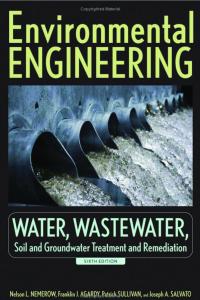
Figure 6. A. Illustration of the seasonal moderator for immigration and emigration, Yseason, for four different latitudes (≥ 63, 56, 45 and 35 °N) and B. The default migration rates for prey and predatory fish (RmigPY and RmigPD, respectively) using data for the Ronneby coastal area (latitude 56 °N)

90


Table 5 gives a compilation of all equations quantifying immigration and emigration. It shows that the basic set-up is applied to all functional groups. Note that CoastWeb does not account for cannibalism (feeding within the functional group). Cannibalism exists in aquatic systems among fish (Menshutkin, 1971), but to gain simplicity, the model calculates net production of fish (and zooplankton and zoobenthos). Table 6 gives all calculated monthly fluxes of predatory fish, i.e., immigration and emigration, initial production (IPR), production (BM/T), fishing and elimination, for the Ronneby coastal area (Table 1). Table 6 and the following four tables give results exemplifying the magnitude of these fluxes. Evidently, uncertainties in major fluxes are more decisive for the predictions than uncertainties in minor fluxes. So, it is important to identify the major fluxes and use algorithms that quantify these as correctly as possible. One can note: The biomass of predatory fish in this coast varies between 2.5 and 4 t wet weight during the year. The initial production is relatively high during summer and fall with a yearly total of 3.2 t/y; the production values are about 3 t/y. Immigration and emigration are significant; immigration 16 t/y and emigration 10 t/y. So, there is a net immigration of predatory fish to this area. The annual fishing of predatory fish under default conditions is 5 t/y. The loss of predatory fish (death, etc.) is 4 t/y. Table 7. gives the corresponding values for prey fish. The biomass of prey fish is about a factor 5 times higher than for predatory fish; the biomass varies between 12 and 20 t during the year. The initial production is 63 t/y and the production about 20 t/y. Immigration is 12 t/y and emigration 25 t/y, which means a significant net outflow of prey fish. Table 6. Calculated monthly and annual values of predatory fish biomass and fluxes of predatory fish in the Ronneby coastal area (southern Baltic Proper) Month Jan Feb Mar Apr May Jun Jul Aug Sep Oct Nov Dec

Biomass (BMPD) (kg ww) 3 811 3 646 3 187 2 647 3 426 3 606 3 828 4 030 4 155 3 977 4 002 3 977 Annual values:

IPRPD (kg ww/m)

ElimPD (kg ww/m)

294 277 240 166 178 229 264 308 329 319 306 304 3 214

365 348 318 260 285 332 347 369 383 381 374 375 4 137

FishingPD (kg ww/m) 128 283 653 1 442 1 010 303 121 91 385 331 139 147 5 033

InmigPD (kg ww/m)

OutmigPD (kg ww/m)

513 622 798 2 096 3 329 2 056 1 422 1 222 1 798 1 060 772 661 16 349

480 432 525 1 100 1 434 1 470 995 869 1 234 846 539 468 10 392

Production (BMPD/TPD) (kg ww/m) 258 246 215 179 231 244 259 272 281 269 270 269 2 993


91

3 906 3 946 4 063 3 907 4 573 5 902 7 147 7 502 6 767 5 912 5 172 4 291 63 088

17 29 43 52 95 150 151 130 102 67 36 14 886

12 18 24 28 56 94 100 84 65 37 21 10 549

1 177 1 107 960 663 713 916 1 056 1 233 1 315 1 278 1 222 1 216 12 856

2 447 2 316 2 136 1 776 1 752 1 911 2 198 2 566 2 738 2 696 2 644 2 569 27 749

287 627 1 460 3 282 2 088 582 256 211 916 783 326 336 11 154

318 341 438 1 782 3 236 1 586 1 041 882 1 241 676 457 379 12 377

1 161 1 252 1 552 2 539 2 533 2 887 2 288 2 179 3 230 2 479 1 673 1 372 25 145

Production (BMPY/TPY) (kg ww/m)

OutmigPY (kg ww/m)

InmigPY (kg ww/m)

FishingPY (kg ww/m)

ElimPY (kg ww/m)

From PY to PD (kg ww/m)

IPRZPPY (kg ww/m)

17 024 16 057 14 516 12 025 12 900 14 338 16 979 19 388 19 366 18 823 18 643 17 845 Annual values:

IPRZHPY (kg ww/m)

Biomass (BMPY) (kg ww)

Jan Feb Mar Apr May Jun Jul Aug Sep Oct Nov Dec

IPRZBPY (kg ww/m)

Month

Table 7. Calculated monthly and annual values of prey fish biomass and fluxes in the Ronneby coastal area

1 727 1 628 1 472 1 220 1 308 1 454 1 722 1 966 1 964 1 909 1 891 1 810 20 071

Zoobenthos is the most dominating and important food for prey fish. The prey fish production from zoobenthos consumption is 63 t/y, compared to 1 t/y from consumption of herbivorous zooplankton and 0.5 t/yr from consumption of predatory zooplankton. The annual fishing of prey fish is 11 t/y. The loss of prey fish (death, etc.) is 28 t/y. Table 8. gives the results for predatory zooplankton. The biomass varies very much during the year, from 120 kg ww during the winter to almost 1.6 t during the summer. The initial production from eating herbivorous zooplankton is over 27 t/yr and the production about 21 t/yr. Immigration is 49 t/y and emigration 40 t/y, i.e., a net inflow from the sea. The elimination is 29 t/y. Table 9 shows the same results for zoobenthos, which feed on benthic algae (430 t/y), macrophytes (24 t/y), but most of all on ―sediments‖ (1000 t/y) since zoobenthos mainly are detrivores. The biomass of zoobenthos varies between 45 and 100 t during the year and is about a factor of 6 higher than the biomass of prey fish. Immigration and emigration are zero (zoobenthos are largely stationary within the given coastal area). The elimination of zoobenthos is about 1000 t/y.

92

Lars Håkanson and Dan Lindgren Table 8. Calculated monthly and annual values of biomass and fluxes for predatory zooplankton in the Ronneby coastal area Month

Jan Feb Mar Apr May Jun Jul Aug Sep Oct Nov Dec

Biomass (BMZP) (kg ww) 117 160 252 340 607 1 159 1 594 1 285 917 681 347 146 Annual values:

IPRZP (kg ww/m)

ElimZP (kg ww/m)

135 150 300 527 933 3 224 6 769 6 676 4 399 2 787 1 051 464 27 415

456 501 790 1 134 1 569 3 309 5 568 5 617 4 182 3 037 1 750 987 28 900

From ZP to JE (kg ww/m) 0 0 0 0 0 0 0 0 0 0 0 0 0

From ZP to PY (kg ww/m) 147 165 259 350 399 814 1 375 1 466 1 222 944 540 306 7 987

InmigZP (kg ww/m) 1 066 1 248 1 926 2 600 3 455 5 994 8 249 7 808 6 376 5 125 3 307 1 983 49 137

OutmigZP (kg ww/m) 626 688 1 084 1 556 2 153 4 542 7 641 7 709 5 739 4 168 2 402 1 355 39 663

Production (BMZP/TZP) (kg ww/m) 323 442 696 940 1 678 3 203 4 405 3 551 2 534 1 882 959 403 21 017

Table 9. Calculated monthly and annual values of biomass and fluxes for zoobenthos in the Ronneby coastal area Month Biomass (BMZB) (kg ww) Jan Feb Mar Apr May Jun Jul Aug Sep Oct Nov Dec

45 501 48 373 53 841 64 705 80 396 100 518 103 515 90 509 77 495 69 738 57 531 47 569 Annual values:

IPRBAZB (kg ww/m) 6 284 10 099 15 137 22 908 49 432 78 805 84 256 68 794 49 825 28 632 15 390 6 157 435 719

IPRsedZB (kg ww/m) 73 156 75 203 76 514 77 983 84 312 91 251 95 216 96 027 94 897 89 079 81 274 73 798 1 008 710

IPRMAZB (kg ww/m) 1 034 1 001 1 069 1 260 1 723 2 510 3 247 3 298 2 876 2 371 1 862 1 280 23 531

From ZB to PY (kg ww/m)

ElimZB (kg ww/m)

24 374 24 720 26 935 33 436 52 251 66 358 75 697 71 336 60 968 40 650 34 077 27 314 538 116

58 168 58 711 60 316 57 851 67 525 86 086 104 025 109 788 99 645 87 189 76 656 63 882 929 844

Production (BMZB/TZB) (kg ww/m) 10 808 11 490 12 789 15 369 19 096 23 876 24 588 21 499 18 407 16 565 13 665 11 299 199 451

These simulations indicate that zoobenthos is an important food for fish in this coastal area and that threats to the production of zoobenthos would be serious to the fish production. Immigration and emigration of fish and zooplankton are important processes. There is generally no jellyfish in the Ronneby coastal area. The next section focuses on jellyfish.

An Outline of the Sub-Model for Jellyfish Jellyfish (JE) can appear in great numbers and are able to consume substantial amounts of mainly zooplankton, which can influence on fish production (Schneider and Behrends, 1994;


93

Brodeur et al., 2002; Purcell, 2003). This makes them an important part of coastal foodwebs and they have been included as a secondary production unit in CoastWeb for areas where the salinity is high enough (the default threshold value in this model is set to 10; Lucas (2001) gave a value of 14 for a common jellyfish, Aurelia aurita). Jellyfish is a predatory zooplankton and could belong to the predatory zooplankton group in the model. However, the medusae-stage, i.e., what we generally mean by jellyfish, is so different compared to other predatory zooplankton concerning size, abundance, etc. that it has been assigned its own group in CoastWeb. Figure 7 illustrates the jellyfish sub-model and Table 10 gives all equations. Although this is a new sub-model, it is built in the same way as all other sub-models. This section will give an outline of this building block. Since jellyfish mainly eat zooplankton (Larson, 1987; Mills, 1995; Hansson, 2006), there is only one food choice between predatory and herbivorous zooplankton. So, the number of first order food choices for jellyfish is NRJE = 2, separated by DCZPZH. Jellyfish are also known to consume ichthyoplankton (fish eggs and larvae; Cowan et al., 1996; Suchman and Brodeur, 2005). However, this is not considered in the model since ichthyoplankton is not included as a functional group. Table 10. Basic differential equation for production and biomass of jellyfish (JE) BMJE(t) IPRZHJE IPRZPJE InmigJE ElimJE OutmigJE FZHJE FZPJE Ychlsea CRJE DCZPZH MERZP RmigJE NJE NBMJE NCRJE SalSW TJE YsalJE Ytemp

= BMJE(t - dt) + (IPRZHJE + IPRZPJE + InmigJE - ElimJE - OutmigJE)·dt = YsalJE· (1- DCZPZH)·FZHJE· MERZP·Ytemp0.5 [initial production of JE from eating ZH] = YsalJE· DCZPZH·FZPJE· MERZP·Ytemp0.5 [initial production of JE from eating ZP] = RmigJE·NBMJEsea [immigration of JE] = BMJE·1.386/TJE [elimination of JE] = RmigJE·BMJE [emigration of JE] = BMJE·CRJE [flux from ZH to JE] = BMJE·CRJE [flux from ZP to JE] = Chlsea/Chlcoast [correction factor for biomasses in the sea and in the coast related to chlorophyll] = (NCRJE+NCRJE·(BMJE/NBMJE-1)) [consumption rate for JE; if NBMJE = 0, then CRJE = 0] = 0.5 [distribution coefficient for JE eating ZP or ZH] = 0.32 [metabolic efficiency ratio for JE eating ZP or ZH] = RmigPY = RmigPD·0.33 [basic migration rates for PY, JE and PD] = 2 [number of first order food choices] = 10·NBMZP = 50·Ychlsea·(1-DCZHZP)·10-6·SMTH((V·38·CTP 0.64),TZP,(V·38·CTP 0.64)) [normal biomass of JE] = NJE/TJE [normal consumption rate for JE] = Surface-water salinity [= 6.5 in the Ronneby coastal area] = 120/30.42 [turnover time for JE in months] = if SalSW < 10 then 0 else 1 [assumed threshold salinity for JE production] = (SWT+0.1)/9 [dimensionless moderator for temperature influences on bioproduction]

94

Lars Håkanson and Dan Lindgren Outline of the sub-model for jellyfish From ZH to JE, FZHJE MERZP

YSWT

T JE

IPR ZHJE

InmigJE

Jellyfish biomass BMJE Elim JE

RmigJE IPR ZPJE

From ZP to JE, FZPJE

OutmigJE CRJE

DCZPZH NCR JE

YsalJE

NJE NBM ZP

NBM JE

SalSW

Figure 7. An outline of the new sub-model for jellyfish

The consumption of biomass from grazing is calculated in kg ww/month. The total consumption is given by FZPJE = BMZP·CRJE. BMZP is the available biomass of predatory zooplankton and CRJE is the actual consumption rate (jellyfish eating its prey): CRJE = (NCRJE+NCRJE·(BMJE/NBMJE-1))

(22)

NCRJE is the normal consumption rate, BMJE is the actual biomass of jellyfish and NBMJE is the normal biomass. This means that the model quantifies changes in the actual consumption of the prey unit related to changes in the biomass of the consumer: more animals in the secondary unit (higher BMJE) means a higher actual consumption rate, CRJE. If the actual biomass of the predator is equal to the normal biomass of the predator, BMJE/NBMJE = 1, and CRJE = NCRJE. If the actual biomass of the predator is twice the normal biomass, then CRJE = 2·NCRJE. So, the model gives a linear increase in consumption with increase in biomass of the secondary unit. Lacking reliable empirical data, it is assumed that NBMJE may be set to be 10 times higher than the normal biomass of predatory zooplankton and depend on salinity. This gives: NBMJE = 10·NBMZP·YsalJE

(23)

By using a boundary condition, NBMJE can never be less than 0. The normal consumption rate, NCRJE, is NCRJE = 2/TJE. TJE is the turnover time of jellyfish (i.e., of the medusae stage). According to Lucas (2001), medusae of the common jellyfish, Aurelia aurita,


95

generally live for 4 to 8 months. In the model, 120 days is used as a default value of turnover time for Jellyfish. The initial production (IPR) of jellyfish (JE) from eating predatory zooplankton (ZP) is given by: IPRJE = YsalJE·DCZPZH·FZPJE·MERZP·Ytemp0.5

(24)

The distribution coefficient, DCZPZH, gives the fraction of predatory zooplankton versus herbivorous zooplankton consumed by jellyfish. The MER-value is the amount of the total consumption (FZPJE) that will increase the biomass of the consumer, here jellyfish. The jellyfish digestion/consumption of its prey is temperature dependent (Martinussen and Båmstedt, 1999). This is accounted for by a dimensionless moderator Ytemp0.5 (Ytemp = ((SWT+0.1)/9); SWT = the SW-temperature in °C). YsalJE is a salinity moderator, which works in the following way: If the SW-salinity (salSW) is lower than 10, then YsalJE = 0 else YsalJE = salSW/10. Jellyfish can in some cases be consumed by fish and turtles (Legović, 1987) and they can also be consumed by other jellyfish (Martinussen and Båmstedt, 1999). However, this is not accounted for in the default set-up of the model. Jellyfish are removed from the coastal system by two processes: elimination, related to the turnover time of jellyfish and emigration. Immigration and emigration of jellyfish are calculated from: FinmigJE = RmigPY·NBMJEsea·YsalJE

(25)

FoutmigJE = RmigPY·BMJE

(26)

The migration rate for jellyfish is set equal to the migration rate for prey fish and the normal biomass of jellyfish in the sea outside the given coastal area is calculated from NBMJEsea = NBMJE·Ychl. The actual biomass of jellyfish in the coastal area, BMJE, is calculated automatically in the model and Ychl is defined by eq. 1. Elimination, i.e. the loss of biomass (ELJE) is given as: ELJE = BMJE·1.386/TJE

(27)

Where 1.386 is the halflife constant (-ln(0.5)/0.5 = (0.693/0.5; see Håkanson and Peters, 1995).

THE ROLE OF MACROPHYTES Macrophyte Cover The sub-model used in LakeWeb to predict the macrophyte cover is shown in eq. 28. MAcovlake = (10.49+1.502·(Sec /Dm)-1.993·(90/(90-Lat))-0. 422·(√Dmax)+0.490·log(A1·10-6))2

(28)

96


In CoastWeb, it has been modified by an energy factor (Yex1) taking into account that coasts are open and affected by wind/wave action from the sea. This moderator quantifies that in coasts, where the wind/wave energy is high and the water exchange fast, it would be more difficult for the roots of the macrophytes to develop which would lower the macrophyte cover (MAcov in % of the coastal area). The macrophyte cover is calculated as: MAcov = MAcovlake· (1/Yex10.75)

(29)

If Ex < 0.003 (lower boundary condition for the exposure; see Figure 1) then Yex1 = 1 else Yex1 = (Ex/0.003)0.25 If Ex > 10 (upper boundary condition for the exposure) then Yex1 = 10 else Yex1 = (Ex/0.003)0.25 So, if the exposure (Ex) is very limited (< 0.003), the equation will calculate the same macrophyte cover as for a lake. If Ex is very high (> 10) for open coasts, (1/Yex10.75) will be 0.18 and the macrophyte cover will be only 18% of the corresponding value for a lake. A typical Ex-value for Baltic coastal areas is about 0.1 (Håkanson, 2006) which gives Yex = 0.52 and a macrophyte cover that is 52% of what would be expected in a lake with the same Secchi depth (Sec in m), the same area above a water depth of one meter (A1 in km2), the same mean depth (Dm in m) and maximum depth (Dmax in m). The macrophyte cover is used to calculate macrophyte production and biomass; the higher the macrophyte cover, the higher the fish biomass (if everything else is constant), since the macrophytes provide a protected environment for small fish (Sogard and Able, 1991). Different macrophyte species prefer different salinities (Boston et al., 1989; King and Garey, 1999) and have different tolerance to changes in salinity (Rout and Shaw, 1998, 2001). A relatively constant salinity is desirable for the macrophytes to abound. Figure 8 shows that the increase in salinity in the middle of the 1990s in Ringkobing Fjord (see Table 1) likely caused the observed reduction in macrophyte cover. There has been a slight change in dominance from sago pondweed Potemogeton pectinatus towards the more salt tolerant ditch grass Ruppia cirrhosa in recent years. This example is included to stress that Coast Web does not include any consideration to the fact that there can be changes in the abundance of single macrophyte species with a higher or lower tolerance to changes in salinity. The overall correspondence between the predicted values for the macrophyte cover during the period when the salinity was lower than 9.5 is good (see Håkanson, 2006), but when the salinity reached a threshold value of 9.5 (Håkanson et al., 2007), there was an initial reduction in macrophytes, which is not captured by the model. This is because when the salinity increases, the Secchi depth will also iincrease, which means that the model will predict an increased macrophyte cover. However, Figure 8 shows that the opposite has happened in Ringkobing Fjord. This indicates that the effect of the changes in salinity on single macrophyte species is even more pronounced than indicated by looking just at the macrophyte cover for the initial period. The actual change should be related to the curve predicted by CoastWeb since these predictions describe what would normally be expected under given conditions related to the factors accounted for in CoastWeb (eq. 28).


97

Figure 8. Illustration of how the mean annual macrophyte cover and the mean annual salinity have varied in Rinkobing Fjord between 1980 and 2004, and how the macrophyte cover is predicted by the modified CoastWeb-model

Macrophytes and Macroalgae and Their Influence on Fish Production Macrophytes and macroalgae constitute a good environment for some species of predatory fish, e.g., for pike to make an ambush (Savino and Stein, 1989). The beds of macrophytes constitute a ―nursery‖ for young fish (Sogard and Able, 1991), which help to sustain a high fish biomass. Macrophytes and macroalgae are generally not important food for most fish (Barnes and Hughes, 1988; except for herbivores), but they provide shelter (Persson and Eklöv, 1995; Duarte, 2000) and can reduce the predation pressure (Nelson and Bonsdorff, 1990; Winfield, 2004), especially on small fish. In LakeWeb, this is handled by a dimensionless moderator, YMA: YMA = (1-0.2·(Maccov/25-1))

(30)

Maccov is the macrophyte cover (%). Macroalgae are expected to play a larger role in saline systems than in lakes for two reasons. Firstly, when the water clarity increases, the depth of the photic zone increases. This increases the production of benthic algae and macrophytes, which can cause a shift from a dominance of pelagic primary production to benthic primary production. Secondly, in marine systems such a shift would likely lead to a higher percentage of large macroalgae compared to smaller benthic algae. These macroalgae will influence the structure of the coastal ecosystem in ways similar to the macrophytes. In LakeWeb, the macrophytes influence the fish production mainly by providing a safe haven for the small fish. This is accounted for by lowering the predation pressure (from man, mammals or birds) on the fish. In CoastWeb, the influence of macroalgae and macrophytes on production and survival of prey and predatory fish is accounted for by a modification of the dimensionless moderator (YMA) in eq. 30. This gives a new moderator YMAcoast, eq. 31, that should reduce the predation pressure on prey and predatory fish in the same manner as YMA does in LakeWeb.

98

Lars Håkanson and Dan Lindgren YMAcoast = YMA/YBAmacro

(31)

YBAmacro is the ratio between the actual biomass of benthic algae in coastal areas and the normal biomass of benthic algae in lakes (YBAmacro = BMBA/NBMBAlake). This ratio reflects the prevalence of macroalgae in coastal areas compared to lakes and is generally higher than 1. In LakeWeb, the loss of prey fish from fishing and predation, is given by a constant default rate. In CoastWeb, the corresponding default rate is modified by two dimensionless moderators meant to make the loss of prey fish from fishing more realistic. The loss of prey fish from fishing is given by FfishPY (in kg ww/month): FfishPY = YMAcoast·BMPY·RfishPY

(32)

BMPY is the biomass of prey fish and RfishPY is the fishing rate of the prey fish. RfishPY is defined as: RfishPY =Ysec·Yseason ·0.5

(33)

0.5 (1/month) is a default fishing rate used in LakeWeb (derived from extensive calibrations), which is affected by two dimensionless moderators that account for influence of Secchi depth (Ysec) and seasonal migration pattern to and from the coastal area (Yseason). If empirical data are available on fishing of prey fish, such data should be used instead of the default fishing rate of 0.5. If the Secchi depth in a corresponding lake (Seclake) is larger than the Secchi depth in the coast (Seccoast = Sec), then Ysec =1 else Ysec = Sec/Seclake. So, if the water clarity in the coast is larger than in a corresponding lake, the predation pressure on prey fish is assumed to be higher than in a lake. This is quantified by this simple dimensionless moderator. Yseason is the dimensionless moderator for seasonal migration (see eq. 19). The loss from all types of predation on predatory fish (FfishPD in kg ww/month) is given in a similar way by: FfishPD = YMAcoast·BMPD·2·RfishPY

(34)

The default assumption is that the rate for fishing and predation is higher for predatory fish than for prey fish based on the fact that large fish are more attractive for professional and recreational fishermen (given by the factor 2). Figure 9 illustrates how the prey fish biomass, the predatory fish biomass and the elimination of prey fish depend on the new algorithm given in eq. 31. In these simulations, the new algorithm was used after month 26, before the algorithm in eq. 30 was used. One should note the effects that the macroalgae would have on the predation of prey fish (Figure 9C). The effect is due to an increase in prey fish biomass, which is compensated for by a significant increase in the food available for predatory fish and hence also in predation pressure of predatory fish on prey fish. The net effect is a relatively small change in prey fish biomass (Figure 9B) and in predatory fish biomass (Figure 9A).


99

Figure 9. Simulations to illustrate the role of macroalgae for the fish production and biomass in coastal areas. In these simulations, the dimensionless moderator expressing how macroalgae influence elimination of prey fish was used from month 26 (the curves ―Accounting for macroalgae‖) compared to a situation when this moderator is not used. Using data from the Ronneby coastal area, S. Sweden, (A) gives the results for predatory fish, (B) for prey fish and (C) for the predation/fishing of prey fish

RESULTS This section presents case-studies to illustrate the potential use of CoastWeb to quantify how three major threats to coastal systems are likely to influence the structure and function of coastal foodwebs and this section will also give results from sensitivity analyses to illustrate how the model works along a latitude/temperature gradient and a salinity gradient. The first case-study focuses on eutrophication, the second on overfishing and the third on toxic contamination.

Eutrophication The idea here is to study how hypothetical stepwise (3-year steps) increases in TP in the sea outside a coast would likely influence the coast. Here, data from the Haverö coastal area are used (Finland; Table 1). The results are presented in Figure 10. The actual (default) TPconcentration in the sea is 24 µg/l, and tests have been done of how values of 0.75·24, 24, 1.5·24 and 2·24 would change modelled values of TP in the coastal water (A), chlorophyll (B), Secchi depth (C), the oxygen saturation in the deep-water zone, O2Sat (D), the normal and actual biomasses of zoobenthos (E), herbivorous zooplankton (F), prey fish (G) and predatory fish (H). Modelled values of TP, chlorophyll, Secchi depth and O2Sat are also

100


compared with empirical data and uncertainty bands for the empirical data. The main results and conclusions of the simulations are: There is generally good correspondence between modelled and empirical data for the TPconcentration (Figure 10A), chlorophyll (Figure 10B), Secchi depth (Figure 10C) and O2Sat (Figure 10D). Note that the empirical chlorophyll value is a mean value for the entire summer period. There is also a close and logical correspondence between the actual and normal biomasses for zoobenthos, herbivorous zooplankton, prey fish and predatory fish. Note that the actual biomasses accounts for seasonal variations and predation more realistically than the normal biomasses, which are basically empirical reference values. The increased hypothetical eutrophication of the sea outside the coastal area will drastically increase TP also in the coast (which is logical because the water retention time in this area is 3-5 days, Persson et al., 1994) (Figure 10E). This leads to higher Chl-values (Figure 10B), reduced Secchi depths (Figure 10C) and lower O2Sat (Figure 10D), which will influence zoobenthos (Figure 10E) living in the sediments more than zooplankton in the more oxygenated surface water (Figure 10F). Since there is much more zoobenthos in the system than zooplankton (about 50 t ww compared to about 3-5 t ww), zoobenthos is an important source of food for omnivorous prey fish and changes in zoobenthos will have clear effects on the prey fish (Figure 10G), and changes in prey fish biomass will in turn influence the predatory fish who feed on prey fish (Figure 10H). The zoobenthos within the accumulation areas (A-areas) will die if O2Sat is lower than 20%, but the oxygenation of the sediments on the erosion and transport areas (ETareas) will maintain a low biomass of zoobenthos in the more shallow parts of the coastal area. To conclude: The increased eutrophication in the sea will imply several changes to the water quality and foodweb characteristics of the studied coastal area. Many of these changes could be expected without a model, but the point here is that they have been quantitatively predicted using a general comprehensive foodweb model which includes a dynamic massbalance model for phosphorus. This modelling accounts for many abiotic and biotic interactions and feedbacks and it is meant to give the ―normal‖ response of the system to the given change in the TP-concentration in the sea. The model accounts for different types of compensatory effects (such as increasing eutrophication leading to a higher primary phytoplankton production, which leads to more suspended particulate matter in the water and a lower Secchi depth, which leads to a smaller depth of the photic zone, which leads to a lower primary phytoplankton production). Such effects are difficult to quantify without a model. As stated, CoastWeb simulates functional groups and hence does not include responses related to single species.


101

Figure 10. Case-study on coastal eutrophication using data from the Haverö coastal area. There are changes in 3-year steps in the TP-concentration in the sea adjacent to the coastal area. The default TPconcentration in the sea is 24 µg l-1 and this value has been set to 0.75·24, 24, 1.5·24 and 2·24 (i.e., 18, 24, 36 and 48 µg l-1) and the consequences calculated for (A) the TP-concentration in the given coastal area, (B) chlorophyll, (C) Secchi depth, (D) oxygen saturation in the deep-water zone (all compared to empirical mean values and inherent uncertainties in the mean values; the chlorophyll mean value is for the summer period) and actual and normal biomasses of (E) zoobenthos (F) herbivorous zooplankton, (G) prey fish and (H) predatory fish. MV: Mean values, SD: Standard deviation

Overfishing Extensive fishing or fishing more than the permitted quota, is, unfortunately, a common practice in most parts of the world and an issue of intensive debate in many countries (Eagle

102


and Thompson Jr., 2003; Hilborn et al., 2003). The idea with this case study is to illustrate how CoastWeb can be used to address this issue. Here, data from the Gävle coastal area (northern Sweden; Table 1) have been used. We will show how changes in fishing would influence the structure of this coastal ecosystem. The scenario is defined in Figure 11A. First, there is a ―normal‖ period of three years, then a period of one year when ten times the normal amount of prey and predatory fish is taken out of the system, followed by a recovery period of two years, then another period of intensive fishing with 20 times the default fishing for a period of two years, followed by a recovery period. Note that this is also a sensitivity analysis since no other changes than fishing have been made. In Figure 11, the consequences for TP-concentration (A), Secchi depth (B), chlorophyll (C) and the actual biomasses with and without this extensive fishing for herbivorous and predatory zooplankton (D, E), zoobenthos (F), prey fish (G) and predatory fish (H) are presented. The main results and conclusions of the simulation are: Also for this coastal area, there is generally a good correspondence between modelled and empirical data for TP (Figure 11A), Secchi depth (Figure 11B) and chlorophyll (Figure 11C). One can also note from these three figures that the changes in fishing in this coastal area would not affect the three water variables very much. There are no clear changes for herbivorous zoolankton (Figure 11D), but increases in the biomass of predatory zooplankton as a response to the lower predatory pressure from a declining biomass of prey fish related to the extensive fishing (Figure 11E and 11G). The lower predation pressure on zoobenthos from a reduced biomass of benthivorous prey fish is evident (Figure 11F). Note that this coastal system will recover quickly. As long as there is fish in the sea outside the coast, immigration of fish will continue, and the system will return to a dynamic steady state, as given by the algorithms for migration in the model. To conclude: The increased fishing will likely only affect the given coastal system marginally and mostly so during the period of the intensive fishing. The immigration of fish from the sea, especially in the springtime, is very large. However, if this kind of fishing were done also in the outside sea, the results would be different. This scenario also shows that it is essential to use as accurate values as possible on immigration and emigration in the model.

Toxic Contamination The final case-study concerns the effects of toxic substances. Our aim is to demonstrate the potential of CoastWeb for making calculations to obtain realistic expectations of the consequences that contaminants can have on the coastal foodweb. We will examine what might happen if a hypothetical contaminant would drastically reduce the biomass of a functional group. Large ecosystem effects should be expected if there are major changes in groups with large biomasses. For that reason, zoobenthos have been selected and data from the Ronneby coastal area have been used. There is also another reason to focus on zoobenthos, related to the fact that many toxic substances show a high affinity for particles in


103

aquatic systems (Håkanson, 1999; Mackay, 2001). This means that high concentrations of such substances may appear in sediments, the habitat for zoobenthos.

Figure 11. Case-study on extensive fishing (or overfishing) using data from the Gävle coastal area. First there is a tenfold increase in the default fishing/predation rate on prey and predatory fish for one year, and then the fishing rate is increased by a factor of 20 for two consecutive years (see Figure A). The consequences of these events are calculated for (A) TP-concentration, (B) Secchi depth and (C) chlorophyll (all compared to empirical data, mean values and uncertainties in the mean values; the chlorophyll mean value is for the summer period). Figures D to H gives a comparison of how this extensive fishing would influence the actual biomasses of (D) herbivorous zooplankton, (E) predatory zooplankton, (F) zoobenthos, (G) prey fish and (H) predatory fish. MV: Mean values, SD: Standard deviation

104


Figure 12. Case-study on toxic contamination using data from the Ronneby coastal area. It is assumed that there is first a contamination that eliminates 90% of the zoobenthos months 7 and 8, then a contamination that kills 99% of the zoobenthos for a whole year, and, finally, total extinction of zoobenthos (see Figure A). The consequences of these events are calculated for the actual and normal biomasses of (B) phytoplankton, (C) benthic algae, (D) bacterioplankton, (E) herbivorous zooplankton, (F) predatory zooplankton, (G) prey fish and (H) predatory fish. MV: Mean values, SD: Standard deviation

Figure 12A presents the scenario. First, 90% of the zoobenthos biomass is reduced (killed by contamination) months 7 and 8, year 4. Then, after a two year recovery period, 99% of the zoobenthos biomass is reduced for an entire year. Finally, after another period of recovery, all zoobenthos are killed. Figure 12 shows how this would influence the actual and normal biomasses of zoobenthos (A), phytoplankton (B), benthic algae (C), bacterioplankton (D), herbivorous zooplankton (E), predatory zooplankton (F), prey fish (G) and predatory fish (H).


105

Initially, there is a good correspondence between actual and normal biomasses also in this area for all the eight functional groups shown in Figure 12. The changes in zoobenthos (Figure 12A) will not affect phytoplankton (Figure 12B), benthic algae (Figure 12C) and bacterioplankton (Figure 12D). Since there is much more zoobenthos in the system than herbivorous and predatory zooplankton (about 100 t ww compared to about 5 and 1 t ww, respectively), zoobenthos is an important food source for omnivorous prey fish and reductions or changes in zoobenthos will have clear effects on prey fish and hence also on predatory fish (compare Figure 12A to Figure 12G and H). To conclude: This case-study shows that a reduction of zoobenthos biomass will have clear effects of fish production and biomass in the given coastal area. This scenario may not be realistic in the sense that nothing but zoobenthos has been affected by the contamination. However, more realistic simulations can be made with the model. The model can, e.g., also be used to simulate non-lethal effects of toxic substances, such as reduced production. The idea here is just to briefly demonstrate its potential.

Sensitivity Analysis – Latitude/Temperature This section first presents a sensitivity analysis along a latitude (temperature) gradient. The latitude for the Gräsmarö coastal area (see Table 1; latitude = 58°N) has been changed in 3-year steps to 40, 50, 58 and 70°N. Results are given in Figure 13 for Secchi depth, TP, O2Sat, chlorophyll (using the general approach in Table 4) and actual and normal biomasses of benthic algae, zoobenthos, prey fish and predatory fish. Figure 13A gives the driving variable, the latitude gradient. The main results and conclusions of the simulation are: The change in latitude will cause clear changes in predicted surface-water temperatures (Figure 13A). There is a good correspondence between modelled and empirical chlorophyll (Figure 13B); the figure gives empirical mean values (MV) and MV plus two standard deviations (SD). There is a good correspondence also between modelled values for sedimentation on accumulation areas and empirical data, as determined from sediment traps (Figure 13C). Figure 14D to H give values of the actual and normal biomasses for phytoplankton, benthic algae, bacterioplankton, zoobenthos and predatory fish. The actual biomasses should give representative values since these values account for predation and several factors that are not included in the calculation of the normal biomasses. In general, however, there is a good correspondence between the two measures indicating that the model works as expected. It is also interesting to compare the biomasses: in this test, the biomass of benthic algae (Figure 13E) is higher than the biomass of bacterioplankton (Figure 13F), which is higher than the biomass of phytoplankton (Figure 13D); the biomass of zoobenthos

106

Lars Håkanson and Dan Lindgren (Figure 13G) is about 20 times higher than the biomass of predatory fish (Figure 13H).

Figure 13. Testing the model along a latitude gradient using data from the Gräsmarö coastal area. The default latitude (58°N) has been changed in 3-year steps by 40, 50, 58 and 70°N and the consequences have been calculated for (A) the surface-water temperature, (B) chlorophyll-a, (C) sedimentation on accumulation areas (as compared to empirical maximum and minimum data from sediment traps), and modelled actual and normal biomasses of (D) phytoplankton, (E) benthic algae, (F) bacterioplankton, (G) zoobenthos and (H) predatory fish. MV: Mean values, SD: Standard deviation


107

Sensitivity Analysis - Salinity This section presents a sensitivity analysis along a salinity gradient. Figure 14 uses data from the Ronneby coastal area (see Table 1). The default salinity inside and outside this area has been increased in 3-year steps from 6.5 to 13, 19.5 and 26 and the consequences calculated for all functional groups and bioindicators while all other factors have been kept constant at the default conditions. Figure 14 gives results for Secchi depth, TP, O2Sat, chlorophyll (using the general approach in Table 4) and actual and normal biomasses of benthic algae, jellyfish, prey fish and predatory fish. Figure 14A gives the driving variable, the salinity gradient. The main results and conclusions are: The increase in salinity will cause a distinct increase in Secchi depth and in water clarity (Figure 14A). There is a good correspondence between modelled and empirical Secchi depths also in this coastal area. Whenever data are available, Figure 14 also gives empirical mean values (MV) and standard deviations for the empirical data (SD) as a measure of the inherent uncertainty in the empirical data. There is a good correspondence between modelled and empirical TP. TP will decrease somewhat along the salinity gradient (Figure 14B). There is also a fine correspondence between modelled and empirical O2Sat, which will decrease with increasing salinity because a high salinity will increase flocculation and sedimentation of suspended particulate matter and particulate phosphoprus. In this open and shallow area, the deep-water turnover time is about 6 days and the deep-water volume is small. This means that the coastal area is well oxygenated (Figure 14C). There is also a relatively good correspondence between modelled and empirical chlorophyll (Figure 14D). Chlorophyll decreases with increasing salinity (see Figure 5) and with lower TP. The biomass of benthic algae (Figure 14E) increases along the salinity gradient because a higher salinity means an increased water clarity and therefore photosynthetic activity. Also the Jellyfish biomass increases (Figure 14F). However, there are no empirical data on biomasses available for comparison. Also the biomass of zoobenthos increases, meaning more food for prey fish and a higher biomass of prey fish along the salinity gradient. More prey fish also means more food for the predatory fish and an increase in predatory fish biomass (Figure 14G and H). The changes in salinity would also influence the migration of fish and the consumption rates since the salinity influences the normal biomasses of both prey and predatory fish. In reality, individual species can be sensitive to changes in salinity and would not survive the big changes in salinity that was used in this example. However, the model does not simulate individual species, but functional groups and a salinity that is non-optimal for one species may be optimal for another species in the same functional group.

108


Figure 14. Testing the CoastWeb-model using data from the Ronneby coastal area along a salinity gradient. The default salinity (6.5) has been increased in 3-year steps by a factor of 1, 2, 3 and 4 and the consequences calculated for (A) Secchi depth, (B) TP-concentration, (C) oxygen saturation in the deepwater zone, (D) chlorophyll-a concentration using the general model (all compared to empirical mean values and inherent uncertainties in the mean values; the chlorophyll mean value is for the summer period) and actual and normal biomasses of (E) benthic algae, (F) jellyfish, (G) prey fish and (H) predatory fish

DISCUSSION AND COMMENTS The overall framework for this modelling is that science and management need practical, operational tools to predict how coastal ecosystems would likely respond to


109

different threats so that the best possible remedial actions can be taken. The model presented in this work in meant as a tool to address such issues. This is exemplified by the case-studies and sensitivity analyses discussed in this paper We have presented a first version of CoastWeb, a coastal foodweb model that simulates ten functional groups and includes a mass-balance model for phosphorus. CoastWeb is an adaptation of a foodweb model for lakes and its underlying structure and main algorithms have been extensively tested. However, this is a first adaptation of the model to coastal conditions and there are several parts that could and should be improved if, and when, better data become available from more coastal areas covering a wide functional domain. At present, the lack of data is most evident for more saline coastal areas. A major deficiency in CoastWeb compared to LakeWeb concerns the empirical models to predict normal biomasses for the functional groups. In this respect, limnology, where good empirical models exist for almost all functional groups, is ahead of coastal ecology. This highlights the importance of getting better data and knowledge on the role of the salinity to predict chlorophyll from phosphorus and/or nitrogen in costal areas. It is also important to seek better knowledge on the processes regulating nitrogen fluxes in marine systems to be able to include a mass-balance model of nitrogen in CoastWeb in the future. In CoastWeb, jellyfish has been introduced as a functional group. The model structure for this group is the same as for all other functional groups. Empirical data have been used for jellyfish model parameterisation, when available. However, in this first version, several estimates have been used that may need to be changed when more and better data become available in the future. Mass occurrence (blooms) of jellyfish also needs to be addressed in future versions of CoastWeb. Due to the high variability that coastal fish show concerning food habits, migratory patterns, etc., it is difficult to develop general algorithms for fish that give good predictions over a wide range of areas. The regional seasonal moderator (Yseason) that handles migration of fish used in this work is only meant as a template and is mainly intended to reflect prevailing conditions in Baltic Sea coastal areas. Similar regional moderators should be developed for other coastal regions. This is especially important since the performed tests show that migration of fish is of major importance for coastal fish biomasses. It is essential to stress that the model simulates functional groups and not individual species. In the presented sensitivity analyses and case-studies, several water variables show good correspondence with existing and available empirical data. The calculated biomasses seem reasonable, but no or few empirical biomasses data have been available to perform independent validations. This is desirable for the future, although it is very hard to get comprehensive, time- and area compatible data on biomasses and abiotic variables from the same area for functional groups of organisms.

ACKNOWLEDGMENTS This work has been carried out within the framework of the Thresholds-project, an integrated EU project (no., 003933-2), and we would like to acknowledge the financial support from EU and the constructive cooperation within the project. Special thanks to prof. Carlos Duarte, the scientific coordinator of the project.

110


APPENDIX: MINOR MODIFICATIONS 1. Salinity is of paramount importance for the number of different species: freshwater species dominate at salinities lower than 5 (psu), brackish water species at salinities from 5 to 20 and saltwater species at higher salinities than 20 (Remane, 1934). The salinity also influences the settling velocity of SPM, and hence water clarity (Secchi depth): the higher the salinity, the greater the aggregation, and the higher the sedimentation (Kranck, 1973, 1979). In CoastMab, this is expressed by a dimensionless moderator for salinity (Ysal) operating on the settling velocity. The effect of salinity is of special importance in estuaries where fresh and saltwater meet and a zone of maximum turbidity occurs (Gebhardt et al., 2005). A new algorithm relating the Secchi depth to SPM and salinity (from Håkanson, 2006) has also been incorporated into CoastWeb. 2. SPM-values are used to calculate the Secchi depth, which in turn is important to predict macrophyte cover and production of benthic algae. In the original CoastMabmodel for total phosphorus (TP) (Håkanson and Eklund, 2007), SPM is calculated by a dynamic SPM-model. For simplicity, and because there is a close relationship between SPM and TP, this version of CoastWeb has omitted the dynamic SPMmodel and uses a regression to predict SPM from dynamically modelled TPconcentrations (Figure 15). It is based on annual data from 51 systems (data from Lindström et al., 1999; Håkanson, 2006) and gives a high coefficient of determination (r2 = 0.895). However, this regression is based on data from systems with salinities lower than 15 so it may provide limited predictive power for systems with higher salinities. y = 1.561x - 1.639; r2 = 0.895; n = 51; p < 0.001 1.75 1.5 1.25

log(SPM) [mg l-1]

1 .75 .5

.25 0

-.25 lake data, salinity 0

-.5 -.75 .6

coastal data, salinity 5-15 .8

1

1.2

1.4

1.6

1.8

2

2.2

2.4

log(TP) [µg l-1] Figure 15. The regression between annual SPM and TP-concentrations based on data from 51 coastal areas and lakes


111

3. The chlorophyll-a concentration (Chl) is important in CoastWeb since Chl is needed to predict phytoplankton biomass. If the aim is to use only CoastWeb, the simplest approach is to use empirical data of Chl. However, if the aim is to study how changes in phosphorus loading affect the foodweb, CoastMab should be linked to CoastWeb. Calculating chlorophyll from nutrients is a fundamental concern in aquatic sciences. Generally, Chl-values are predicted from temperature or light and nutrient concentrations (Dillon and Rigler, 1974; Smith, 1979; Riley and Prepas, 1985; Evans et al., 1996). In this work, regressions relating monthly TP to monthly chlorophyll are used. A local relationship (Håkanson et al., 2007) between chlorophyll and TP has been used for Ringkobing Fjord, Denmark (see Table 4 and Figure 16, with and without a smoothing function SMTH; see Håkanson, 1999). Note that modelled values are not compared to the empirical mean values, but to uncertainty bands calculated as median monthly values ± the uncertainty in the mean empirical value. The regional regression in Table 4 is from Håkanson and Eklund (2007); (SWT+0.1)/20) is the temperature moderator where 20°C is the summer mean temperature for this regression. If no local or regional relationships are available, the general approach in Table 4 may be used. This is an adaptation of a basic regression for lakes [(0.28·CTP)0.96; from OECD (1982)], which is modified by a four moderators. The calcium moderator (YCa) takes into account that systems with Caconcentrations > 10 mg/l are likely to have lower Chl-values relative to TP than systems with lower Ca-concentrations (Håkanson et al., 2005). The morphometry moderator, YDRchl, quantifies how the dynamic ratio (DR = √Area/Dm; Area in km2 and mean depth, Dm, in m) influences the relationship between TP and Chl. Systems with DR > 2.45, are dominated by resuspension events of fine sediments (Håkanson and Jansson, 1983). In such systems, benthic algae may be resuspended and included in the water sample used for the chlorophyll analysis. YDRchl is given by: If DR < 2.45 then YDRchl = 1 else YDRchl = DR/2.45

(35)

The temperature moderator [Ytemp= ((SWT+0.1)/20)] has already been mentioned. The salinity moderator, Ysal, takes into account that the salinity influences the distribution coefficient between dissolved and particulate P in a similar way as calcium: the higher the salinity the lower the slope of the regression line between TP and chlorophyll (Figure 5; Håkanson et al., 2007). The relationship between Chl and phosphorus is also affected by the particulate fraction of phosphorus (PF). In LakeWeb, monthly PF was set to 0.56 as a reference value (Håkanson and Eklund, 2007), but in CoastWeb PF is affected by the biouptake and retention of phosphorus in functional groups, eq. 36. If SWT > 9 °C then PF = 0.56·(MSW + Mshort + Mlong)/MSW else PF = 0.56·MSW/(MSW+ Mshort + Mlong)

(36)

MSW, Mshort, Mlong are the amounts of TP [g] in the surface water, in functional groups with short turnover times and with long turnover times. So, in CoastWeb,

112

Lars Håkanson and Dan Lindgren dynamically modelled TP-concentrations can be used to predict chlorophyll using the best available empirical regressions. 4. The volume of the deep-water (DW) zone, VDW, is not calculated from Awb·(DmaxDwb)/3 (Awb = the area below the theoretical wave base in m2; Dmax = the maximum depth in m; Dwb = the depth of the theoretical wave base in m), as it was in LakeWeb, but from: VDW = Awb·Vd·(Dmax-Dwb)/3

(37)

The previous expression works well for systems where the DW-zone has the form of a cone, but for systems that are more U-shaped with Vd-values higher than 1, the correction using the form factor (Vd = 3·Dm/Dmax) will provide a more realistic estimate of VDW. 5. The moderator, YEh1, is used to express the oxygen stress on zoobenthos in LakeWeb. In CoastWeb, it has been replaced by a more tested approach, which is also used to quantify diffusion of phosphorus from sediments (Håkanson and Eklund, 2007): If O2Sat > 50% then YEh1 = (2-1·(O2Sat/50-1)) else YEh1 = (2-3000·(CTPA/1)·(O2Sat/50-1))

(38)

Figure 16. Modelling chlorophyll in Ringkobing Fjord, from modelled monthly TP-concentrations (actual data and smoothed data) using the CoastMab-model (within CoastWeb) and the regression given in eq. 2, compared to uncertainty bands based on median monthly values ± the uncertainty in the empirical annual mean values (see Håkanson et al., 2007)


113

CTPA is the modelled TP-concentration is accumulation-area (A) sediments. If CTPA is higher than 1 mg/g dw, the dimensionless amplitude value (3000) increases, and hence also the diffusion; if CTPA is lower than 1, the amplitude value decreases. The following smoothing function has also been applied to provide realistic temporal changes in the moderator for zoobenthos: YEh = SMTH(1/YEh1, TZB, 1/YEh1)

(39)

TZB is the turnover time for zoobenthos (Table 2). YEh is never permitted to attain values < 0. 6. The dimensionless moderator expressing how low oxygen saturation in the DW-zone (O2Sat in %) would influence the survival of zoobenthos in areas of erosion and transport (ET-areas) has been modified from YEh10.25 to YEh10.5. This means that a low O2Sat will more clearly reflect lower oxygen conditions also in the surface water. 7. The distribution coefficient regulating the prey fish consumption of either zooplankton or zoobenthos has been changed from 0.5 in LakeWeb to DCZPZB = 0.5·Ysec0.2. For coasts, which generally have a higher water clarity than lakes, the basic DC-value is modified by a Secchi depth moderator (Ysec;, eq. 40), that compares the Secchi depth in the coast Secchicoast with that of a corresponding lake, Secchilake. If Secchilake > Secchicoast then Ysec = 1 else Ysec = Secchicoast/Secchilake

(40)

Which, e.g., gives 0.5·20.2 = 0.57 (a diet of 57% zooplankton and 43% zoobenthos consumed by prey fish) if Ysec is 2. The power (0.2) has been derived by calibration. 8. The moderator used in LakeWeb to reduce the predation pressure in very turbid lakes (Yfish) has been set to 1, since Secchi depths lower than 1 m are rare in coastal areas on a monthly basis (the ecosystem scale). 9. The amount of food (―sediment pool‖, FsedZB in kg ww/month) available for the zoobenthos is not calculated in the same manner as in LakeWeb, but from sedimentation of particulate phosphorus recalculated into sedimentation of organic matter as food for the zoobenthos. This is done accordingly: FsedZB = FAET·(1000/2)·1000·(100/(1-W))·0.67

(41)

FAET is the sedimentation of TP on ET- and A-areas in g dw/month (calculated automatically in CoastMab from eq. 42). FAET is calculated from a function which gives an annual smoothing of the monthly sedimentation on ET-areas and A-areas (FSWET and FDWA in g TP/month): FAET = SMTH((FSWET+FDWA), 12, (FSWET+FDWA))

(42)

From Håkanson (2006) it is assumed that SPM deposited on ET- and A-areas on average has a TP-concentration of 2 mg/g dw. Multiplication with 1000 gives SPM in kg dw/month. W is the water content of SPM (= 100·(g ww-g dw)/g ww) of SPM

114

Lars Håkanson and Dan Lindgren calculated from eq. 43. Multiplication with (100/(1-W)) gives the amount of SPM in kg ww/month. It is also assumed that 2/3 of the deposited SPM is available as food for zoobenthos. W = (1-0.0375·(ET/0.15-1))·75

(43)

When the fraction of ET-areas is 15%, W is 75% which is used as the default water content of ET- and A-sediments in coastal areas (Håkanson et al., 1984). If the fraction of ET-areas (with coarser materials), is higher, the calculated water content of the SPM should be lower, which is given by eq. 43. If ET is 0.9, W is 61%.

REFERENCES Axenrot, T. & Hansson, S. (2004). Seasonal dynamics in pelagic fish abundance in a Baltic Sea coastal area. Estuar. Coast. Shelf Sci., 60, 541-547. Barnes, R. S. K. & Hughes, R. N. (1988). An introduction to marine ecology, 2nd ed. Blackwell Scientific Publications, Oxford, 351. Boston, H. L., Adams, M. S. & Madsen, J. D. (1989). Photosynthetic strategies and productivity in aquatic systems. Aquat. Bot., 34, 27-57. Brodeur, R. D., Sugisaki, H. & Hunt, G. L. Jr., (2002). Increases in jellyfish biomass in the Bering Sea: implications for the ecosystem. Mar. Ecol. Prog. Ser., 233, 89-103. Christensen, V., Walters, C. J. & Pauly, D. (2000). Ecopath with Ecosim: A User‘s Guide. Fisheries Centre, Univ. of British Columbia, Vancouver, 130. Cowan, J. H., Jr, Houde, E. D. & Rose, K. A. (1996). Size-dependent vulnerability of marine fish larvae to predation: an individual-based numerical experiment. ICES J. Mar. Sci., 53, 23-37. Dillon, P. J. & Rigler, F. H. (1974). The phosphorus-chlorophyll relationship in lakes. Limnol. Oceanogr, 19, 767-773. Duarte, C. M. (2000). Marine biodiversity and ecosystem services: an elusive link. J. Exp. Mar. Biol. Ecol., 250, 117-131. Eagle, J. & Thompson Jr., B. H. (2003). Answering Lord Perry‘s question: dissecting regulatory overfishing. Ocean Coast. Manag., 46, 649-679. Evans, M. S., Arts, M. T. & Robarts, R. D. (1996). Algal productivity, algal biomass, and zooplankton biomass in a phosphorus-rich, saline lake: deviations from regression model predictions. Can. J. Fish. Aquat. Sci., 53, 1048-1060. Gebhardt, A. C., Schoster, F., Gaye-Haake, B., Beeskow, B., Rachold, V., Unger, D. & Ittekkot, V. (2005). The turbidity maximum zone of the Yenisei River (Siberia) and its impact on organic and inorganic proxies. Estuar. Coast. Shelf Sci., 65, 61-73. Hansson, L. J. (2006). A method for in situ estimation of prey selectivity and predation rate in large plankton, exemplified with the jellyfish Aurelia aurita (L.). J. Exp. Mar. Biol. Ecol., 328, 113-126. Harvey, C. J., Cox, S. P., Essington, T. E., Hansson, S. & Kitchell, J. F. (2003). An ecosystem model of food web and fisheries interactions in the Baltic Sea. ICES J. Mar. Sci., 60, 939-950.


115

Håkanson, L. (1999). Water pollution - methods and criteria to rank, model and remediate chemical threats to aquatic ecosystems. Backhuys Publishers, Leiden, 299. Håkanson, L. (2000). Modelling radiocesium in lakes and coastal areas - new approaches for ecosystem modelers. A textbook with Internet support. Kluwer Academic Publishers, Dordrecht, 215. Håkanson, L. (2006). Suspended particulate matter in lakes, rivers and marine systems. The Blackburn Press, New Jersey, 331. Håkanson, L., Blenckner, T., Bryhn, A. C. & Hellström, S. S. (2005). The influence of calcium on the chlorophyll-phosphorus relationship and lake Secchi depths. Hydrobiologia, 537, 111-123. Håkanson, L. & Boulion, V. V. (2002). The Lake Foodweb - modelling predation and abiotic/biotic interactions. Backhuys Publishers, Leiden, 344. Håkanson, L., Bryhn, A. C. & Eklund, J. M. (2007). Modelling phosphorus and suspended particulate matter in Ringkobing Fjord in order to understand regime shifts. J. Mar. Syst., 68, 65-90. Håkanson, L. & Eklund, J. M. (2007). A dynamic mass balance model for phosphorus fluxes and concentrations in coastal areas. Ecol. Res., 22, 296-320. Håkanson, L. & Gyllenhammar, A. (2005). Setting fish quotas based on holistic ecosystem modelling including environmental factors and foodweb interactions – a new approach. Aquat. Ecol., 39, 325-351. Håkanson, L. & Jansson, M. (1983). Principles of lake Sedimentology, Springer, Berlin, 316. Håkanson, L. & Karlsson, M. (2004). A dynamic model to predict phosphorus fluxes, concentrations and eutropications effects in Baltic coastal areas. In: M. Karlsson, Predictive modelling – a tool for aquatic environmental management. Thesis, Department of Earth Sciences, Uppsala University, 108. Håkanson, L., Kulinski, I. & Kvarnäs, H. (1984). Vattendynamik och bottendynamik i kustzonen. SNV PM 1905, Solna, 228. (in Swedish). Håkanson, L. & Peters, R. H. (1995). Predictive limnology. Methods for predictive modelling. SPB Academic Publishing, Amsterdam, 464. Hilborn, R., Branch, T. A., Ernst, B., Magnusson, A., Minte-Vera, C. V., Scheuerell, M. D. & Valero, J. L. (2003). State of the Worlds Fisheries. Annu. Rev. Environ. Resour., 28, 359399. King, G. M. & Garey, M. A. (1999). Ferric Iron Reduction by Bacteria Associated with the Roots of Freshwater and Marine Macrophytes. Appl. Environ. Microbiol, 65, 4393-4398. Kranck, K. (1973). Flocculation of suspended sediment in the sea. Nature, 246, 348-350. Kranck, K. (1979). Particle matter grain-size characteristics and flocculation in a partially mixed estuary. Sedimentology, 28, 107-114. Larson, R. J. (1987). Daily ration and predation by medusae and ctenophores in Saanich inlet, B.C., Canada. Neth. J. Sea Res., 21, 35-44. Larsson, S. & Berglund, I. (2005). The effect of temperature on the energetic growth efficiency of Arctic charr (Salvelinus alpinus L.) from four Swedish populations. J. Therm. Biol., 30, 29-36. Legović, T. (1987). A recent increase in Jellyfish populations: A predator-prey model and its implications. Ecol. Model., 38, 243-256. Levinton, J. S. (2001). Marine biology: function, biodiversity, ecology, 2nd Ed. Oxford University Press, New York, USA, 515.

116


indström, M., Håkanson, L., Abrahamsson, O. & Johansson, H. (1999). An empirical model for prediction of lake water suspended matter. Ecol. Model, 121, 185-198. Lucas, C. H. (2001). Reproduction and life history strategies of the common jellyfish, Aurelia aurita, in relation to its ambient environment. Hydrobiologia, 451, 229-246. Mace, P. M. (2001). A new role for MSY in single-species and ecosystem approaches to fisheries stock assessment and management. Fish and Fisheries, 2, 2-32. Mackay, D. (2001). Multimedia Environmental Models. The Fugacity Approach, 2nd ed. Lewis Publishers, Boca Raton, FL, USA, 272. Martinussen, M. B. & Båmstedt, U. (1999). Nutritional ecology of gelatinous planktonic predators. Digestion rate in relation to type and amount of prey. J. Exp. Mar. Biol. Ecol., 232, 61-84. Menshutkin, V. V. (1971). Mathematical modelling of populations and communities of aquatic animals. Leningrad (in Russian). Mills, C. E. (1995). Medusae, siphonophores, and ctenophores as planktivorous predators in changing global ecosystems. ICES J. Mar. Sci., 52, 575-581. Moen, F. E. & Svensen, E. (2004). Marine fish and invertebrates. AquaPress, Essex, 608. Monte, L. (1995). A simple formula to predict approximate initial contamination of lake water following a pulse deposition of radionuclide. Health Phys., 68, 397-400. Monte, L. (1996). Collective models in environmental science. Sci. Total Env., 192, 41-47. Monte, L., Brittain, J. E., Håkanson, L. & Gallego, E. (1999). MOIRA models and methodologies for assessing the effectiveness of countermeasures in complex aquatic systems contaminated by radionuclides. ENEA, RT/AMP, 150. Nelson, W. G. & Bonsdorff, E. (1990). Fish predation and habitat complexity: are complexity thresholds real? J. Exp. Mar. Biol. Ecol., 141, 183-194. OECD. (1982). Eutrophication of waters. Monitoring, assessment and control. OECD, Paris, 154. Persson, J., Håkanson, L. & Pilesjö, P. (1994). Prediction of surface water turnover time in coastal waters using digital bathymetric information. Environmetrics, 5, 433-449. Persson, L. & Eklöv, P. (1995). Prey refuges affecting interactions between piscivorous perch and juvenile perch and roach. Ecology, 76, 70-81. Peters, R. H. (1991). A Critique for Ecology. Cambridge Univ. Press, Cambridge, 366. Pilesjö, P., Persson, J. & Håkanson, L. (1991). Digital sjökortsinformation för beräkningar av kustmorfometriska parametrar och ytvattnets utbytestid. National Swedish Environmental Protection Agency (SNV) Report no. 3916, Solna, Sweden, 76. (in Swedish). Purcell, J. E. (2003). Predation on zooplankton by large jellyfish, Aurelia labiata, Cyanea capillata and Aequorea aequorea, in Prince William Sound, Alaska. Mar. Ecol. Prog. Ser., 246, 137-152. Remane, A. (1934). Die Brackwasserfauna. Verh. Dtsch. Zool. Ges., 36, 34-74. Riley, E. T. & Prepas, E. E. (1985). Comparison of the phosphorus-chlorophyll relationships in mixed and stratified lakes. Can. J. Fish. Aquat. Sci., 42, 831-835. Rout, N. P. & Shaw, B. P. (1998). Salinity tolerance in aquatic macrophytes: probable role of proline, the enzymes involved in its synthesis and C4 type of metabolism. Plant Sci., 136, 121-130. Rout, N. P. & Shaw, B. P. (2001). Salt tolerance in aquatic macrophytes: possible involvement of the antioxidative enzymes. Plant Sci., 160, 415-423.


117

Sandberg, J., Elmgren, R. & Wulff, F. (2000). Carbon flows in Baltic Sea food webs – a reevaluation using a mass balance approach. J. Mar. Syst., 25, 249-260. Savino, J. F. & Stein, R. A. (1989). Behavioural interactions between fish predators and their prey: effects of plant density. Animal Behav, 37, 311-321. Schneider, G. (1989). Estimation of food demands of Aurelia Aurita medusae populations in the Kiel Bight/Western Baltic. Ophelia, 31, 17-27. Schneider, G. & Behrends, G. (1994). Population dynamics and the trophic role of Aurelia aurita medusae in the Kiel Bight and western Baltic. J. Mar. Sci., 51, 359-367. Smith, V. H. (1979). Nutrient dependence of primary productivity in lakes. Limnol. Oceanogr, 24, 1051-1064. Sogard, S. M. & Able, W. (1991). A comparison of eelgrass, sea lettuce macroalgae, and marsh creeks as habitats for epibenthic fishes and decapods. Estuar. Coast. Shelf Sci., 33, 501-519. Suchman, C. L. & Brodeur, R. D. (2005). Abundance and distribution of large medusae in surface waters of the northern California Current. Deep-Sea Res., II 52, 51-72. Vollenweider, R. A. (1968). The scientific basis of lake eutrophication, with particular reference to phosphorus and nitrogen as eutrophication factors. Tech. Rep., DAS/DSI/68.27, OECD, Paris, 159. Wallin, M., Håkanson, L. & Persson, J. (1992). Belastningsmodeller för närsaltutslepp i kustvatten – speciellt fiskodlingars miljöpåverkan. Nordiska ministerrådet, 1992, 502, Copenhagen, 207 (in Swedish). Walters, C. J., Christersen, V. & Pauly, D. (1997). Structuring dynamic models of exploited ecosystems from trophic mass-balance assessments. Rev. Fish Biol. Fish., 7, 139-172. Walters, C. J., Christersen, V., Pauly, D. & Kitchell, J. F. (2000). Representing density dependent consequences of life history strategies in aquatic ecosystems: Ecosim II. Ecosystems, 3, 70-83. Winberg, G. G. 1985). Main features of production process in the Naroch lakes. Ecological system of Naroch lakes. Minsk, 269-284 (in Russian). Winfield, I. J. (2004). Fish in the littoral zone: ecology, threats and management. Limnologica, 34, 124-131.

In: Lagoons: Biology, Management and Environmental Impact ISBN: 978-1-61761-738-6 Editor: Adam G. Friedman, pp. 119-151 © 2011 Nova Science Publishers, Inc.

Chapter 4

FORM AND FUNCTIONING OF MICRO SIZE INTERMITTENT CLOSED OPEN LAKE LAGOONS (ICOLLS) IN NSW, AUSTRALIA

1

W. Maher1, K. M. Mikac2, S. Foster1, D. Spooner1 and D. Williams1

Ecochemistry Laboratory, Institute for Appled Ecolgy, University of Canberra, Bruce, ACT, Australia. 2 Institute for Conservation Biology and Environmental Management, University of Wollongong, Wollongong, NSW, Australia.

ABSTRACT ICOLLs are considered to be one of the most ecologically productive ecosystems on earth. Similar to other coastal water bodies, ICOLLs lie at the interface of marine, freshwater and terrestrial systems and therefore represent highly dynamic transition zones between river/creek catchments and near-shore coastal waters. ICOLLs often act as net sinks of land derived sediments and nutrients; mature systems are believed to act as a source of organic material and nutrients to the adjacent sea. Suzuki et al., (1998) describes ICOLLs as having unique structural and functional characteristics as a consequence of their position in the landscape, thus having large spatial and temporal variability in their environmental and (consequently their dependant) biological variables. The focus for this chapter is micro size ICOLLs, classified as any coastal water body that has: (i) the presence of barrier beach, spit or series of barrier islands that can restrict oceanic exchange; (ii) a surface water area of less than 0.5 km2 (iii) the retention of all or the majority of the water mass within the lagoon during low tide in the adjacent sea; and (iv) the capacity of to remain brackish to fully saline either by percolation through and/or overtopping through inlet/outlet channels.

120

W. Maher, K. M. Mikac, S. Foster et al. ICOLLs can be viewed in a hierarchical manner, with the ocean and catchment influencing other smaller scale processes. Characteristics of the catchment and oceanic regimes influence water quality, tidal regime, stream flow, sediment delivery and seston within an ICOLL. Flow regimes and sediment loads in turn affect ICOLL morphology and sediment composition, such as nutrient status and organic matter composition. Alterations in catchment flow can either increase the residence time of water within an ICOLL increasing the susceptibility to eutrophication or decrease the residence time possibly leading to nutrient limiting conditions. In turn, these attributes determine the biological diversity and functioning of these systems.

1. INTRODUCTION AND DEFINITION Intermittently Closed and Open Lake Lagoons (ICOLLs) are a common feature of the NSW coastline, occupying approximately 92 % of all New South Wales estuarine waters (Williams et al., 1998). ICOLLs are coastal bodies of saline water (Figure 1), either wholly or partially separated from the adjacent sea, by one or more restricted inlets (Bird, 1967a, b, 1994; Mee, 1978). They are characterised as having largely varying salinities e.g. hyposaline to hypersaline (Kjerfve, 1986, 1994; Bamber, 1998), and often as being stagnant and brackish (ie: 5-20ppt) in nature (Ward and Ashley, 1989; Tagliapietra et al., 2009). ICOLLs are considered to be one of the most ecologically productive ecosystems on earth (Boynton et al., 1996). Similar to other coastal water bodies, ICOLLs lie at the interface of marine, freshwater and terrestrial systems and therefore represent highly dynamic transition zones between river/creek catchments and near-shore coastal waters (Edgar and Barrett, 2000). ICOLLs often act as net sinks of land derived sediments and nutrients; mature systems are believed to act as a source of organic material and nutrients to the adjacent sea (Kjerfve and Magill, 1989; Cognetti and Maltagliati, 2000). Suzuki et al., (1998) describes ICOLLs as having unique structural and functional characteristics as a consequence of their position in the landscape, thus having large spatial and temporal variability in their environmental and (consequently their dependant) biological variables. On the south eastern coast of NSW they provide a habitat for commercially important fish stocks (Griffiths, 2001), and are sanctuaries for many migrating demersal nektonic species (e.g. shrimps, crabs, spots, flounders) that depend on shallow lagoonal habitats as nursery areas for early development (Boynton et al., 1996). Of all the systems that are inherent to the coastal environments, ICOLLs have the greatest potential to become eutrophic (Comin and Valiela, 1993; Boynton et al., 1996; Menendez and Comin, 2000). Reduced flushing, shallow waters, and often silt/clay sediment composition all contribute to accelerate eutrophication. NSW coastal lakes are under immense pressure, and almost all have been modified with approximately 60% classified as degraded and in need of comprehensive or significant protection (HRC, 2002). One of the main problems associated with this assessment was the lack of data for micro size ICOLLs along the south coast of NSW, which highlight the requirement for future research priority. To provide the focus for this chapter a micro size ICOLL will be classified as any coastal water body that has:

Form and Functioning of Micro Size Australian Intermittent Closed Open Lake… 121 (i) the presence of barrier beach, spit or series of barrier islands that can restrict oceanic exchange; (ii) a surface water area of less than 0.5 km2 (iii) the retention of all or the majority of the water mass within the lagoon during low tide in the adjacent sea; and (iv) the capacity of to remain brackish to fully saline either by percolation through and/or overtopping through inlet/outlet channels.

Figure 1. Morphology and sediment facies of micro-size ICOLLs. A: Brackish Creeks (Wimbie Creek); B: Broad Basins (Kianga Lake); C: Floodplain brackish creeks (Congo Creek)

122

W. Maher, K. M. Mikac, S. Foster et al.

Figure 2. Hierarchical effects in ICOLLs

ICOLLs can be viewed in a hierarchical manner; with the ocean and catchment influencing other smaller scale processes (see Figure 2). Characteristics of the catchment and oceanic regimes influence water quality, tidal regime, stream flow, sediment delivery and plankton within an ICOLL (Kench 1999; Loneragan and Bunn 1999; Roshanka and Pattiaratchi 1999; Cooper 2001; Roy et al. 2001). Flow regimes and sediment loads in turn affect ICOLL morphology and sediment composition, such as nutrient status and organic matter composition (Harris 2001b). In turn, these attributes determine the biological diversity and functioning of these systems. Alterations in catchment flow can either increase the residence time of water within an ICOLL increasing the susceptibility to eutrophication or decrease the residence time possibly leading to nutrient limiting conditions (Cooper 2001).

2. PHYSICAL FEATURES ICOLLs are located at the transitional zone between rivers and oceans and often act as net sinks of land derived sediment and nutrient inputs (Kennish, 1986; Kjerfve, 1994). ICOLLs may have one or multiple entrances to the sea that are intermittently open or closed to the ocean (Kench, 1999). These shallow systems are often found behind barrier islands and sand spits and are conspicuous physiographic features of continental land margin around the world (Boynton et al., 1996). The movement of sediment into these water bodies is part of an evolutionary process and changes the morphology and bathometry of the ICOLL basin (Kennish, 1986). Accelerated

Form and Functioning of Micro Size Australian Intermittent Closed Open Lake… 123 infilling caused by increased catchment sediment loads can sometimes ‗in fill‘ coastal ICOLLs, although the isolation of the water body from the ocean is the true cause of their demise (Hodgkin, 1998). The different stages of isolation of ICOLLs to the ocean have also been attributed to differences in ICOLL volume and varying catchment discharges (i.e. sporadic or consistent) (Hodgkin, 1998). The location of the ICOLL entrance in relation to the inherent coastal features that shelter them from prevailing wind and ocean waves is also an important physical aspect of ICOLLs (Hodgkin, 1998). The formation of the barrier that restricts oceanic exchange is reliant on shoreline drift of marine sands that accumulate at the entrance of the ICOLL (Kennish, 1986). During high river discharges the barrier can be breached allowing tidal inflow and exchange. Understanding of the ecological and hydrological consequences of these breaches within south eastern Australian ICOLLs are limited (Pollard, 1994; Wiecek and Floyd, 2006; Gale et al., 2007). In Australia, ICOLLs are found where high wave energy, microtides (ie: tidal amplitude 95% in 24 hours) was reached with an acetic acid to H2O2 mole ratio of 3.

CASE STUDIES The oxidizers mentioned above show different effectiveness in treating sediments, according to the pollutants, the sediment and the environmental conditions involved. Experimental tests are recommended to assess site-specific feasibility of chemical oxidation and to select the most appropriate treatment conditions [Huling et al., 2006; Rivas, 2006]. Two case studies are discussed in this chapter, for which chemical oxidation was tested at lab scale on polluted sediments from Porto Marghera (Venice, Italy) and New York/New Jersey Harbor (NY, USA). In the first case, Fenton-like reagents were used to treat total petroleum hydrocarbons (TPHs), PAHs, and PCBs. In the second case, different oxidizers (Fenton-like reagents, chemically activated persulfate, and peroxy-acid) were tested on sediments with high PAH concentrations, also assessing under selected conditions changes in metal leachability and Specific Resistance to Filtration (SRF) of the treated sediments.

MATERIALS AND METHODS Sediments Porto Marghera Sediments Located next to Venice lagoon, Porto Marghera is one of the most important industrial/commercial harbors in Italy. From the 1950s to 1980s, many chemical and petrochemical industries have settled at the site, but after this period, the recognition of human health hazards due to pollution brought to the progressive reduction of industrial activities. In 1993, a protocol was signed by the local authorities and the Italian Environmental Ministry, establishing specific limit values for the sediments dredged in the lagoon. According to this protocol, the final destination of the dredged sediments must take into account pollutant concentrations. In 1998, Porto Marghera was recognized as a National Priority Site (NPS) by the Italian Law n° 426. An official agreement was signed between different public institutions and private companies to remediate the site [Carlon et al., 2005]. The sediments used for this study were dredged in the Northern canal. To ensure the stability of their physical-chemical properties over the duration of the research program (2 years), after dredging the material has been air-dried for 72 hours, sieved to less than 4 mm to remove wood and shells, homogenized, and stored under controlled conditions.

286

Sabrina Saponaro, Alessandro Careghini, Kevin Gardner et al.

The sediment was composed of sand (39  2 % w./w.) and particles 100 μm). Fractions lesser than 100 μm were analyzed by photosedimentation (MicromeriticsR SediGraph 5100 ET). Na-hexametaphosphate has been used as a dispersing agent. The mineralogical analysis of samples was carried out by means of X-ray diffraction (XRD) using a Siemens D-5000 equipment with a scanning speed of 102θ/min and Cu-kα radiation. XRD studies were performed both on randomly oriented samples (total fraction) and clay fraction samples (< 2 µm), the last prepared from cation-saturated, ultrasonic treated suspensions oriented on glass slides. The identification of the clay fraction minerals was carried out on oriented Mg2+-saturated samples with ethylene glycol salvation, and also after

374

F. Ruiz, M. Pozo, M. I. Carretero et al.

heating at 5500C following K+ saturation. When required, carbonates were eliminated using 0.6 N acetic acid. Quantitative estimation of the mineral content was carried out using the intensity factors calculated by Schultz (1964) and Barahona (1974). Results from 65 bulk samples and 41 oriented clay samples are shown in Tables 1 and 2, respectively.

Figure 1. Geographical setting and geomorphology of the Doñana National Park, with location of the cores

Birth, Evolution and Death of a Lagoon: Late Pleistocene to Holocene…

Figure 2. Long Cores. Distribution of facies and mineralogical samples

Figure 3. Short cores. Distribution of facies and mineralogical samples

375

376

F. Ruiz, M. Polzo, M. I. Carretero et al.

In addition, the >63 µm fraction was revised under stereoscopic microscope, in order to effectuate a general revision of the palaeontological record. This revision includes the taxonomical determination and the estimation of both densities and diversities of bivalves, gastropods, ostracods and foraminiferids. In addition, the presence and relative abundance of other groups (scaphopods, barnacles, bryozoans, crabs) have been also detailed.

3.2. Mathematical Procedures A multivariate analysis was applied to determine the mineralogical sample groups based on the percentages computed of the main minerals (quartz, calcite, phyllosilicates, feldspars and dolomite). An initial clustering procedure is applied using a hierarchical agglomerative technique with the application of the Euclidean distance and the Ward linkage. Results are contrasted by discriminant analysis, by determining both the dimensions and variables on which the groups differ. In addition, a stepwise selection procedure was computed and the contribution of each of the predictor variables to the overall discrimination was determined. The error rate estimation was obtained by a final cross-validation method. These statistical techniques were carried out using several subprograms of the Statistical Package for the Social Sciences (SPSS™). Further details of these techniques may be consulted in Dillon and Goldstein (1984).

3.3. Radiocarbon Chronology Two new dates were produced at the Beta Analytic Laboratory (Miami, USA) by radiocarbon analysis of mollusc shell (Figure 6. core CM), whereas the remaining twelve dates were obtained from Ruiz et al. (2004; 2005 a, b) and Pozo et al. (2010). All data were calibrated using CALIB version 5.0.2 (Stuiver and Reimer, 1993) and the Stuiver et al. (1998) calibration dataset. The final results correspond to calibrated ages (ca.) using 2σ intervals, with the reservoir corrections suggested by Soares and Dias (2006 a, b) and Soares (2008) for this area. For the time interval 4500-4000 yr BP, more future results are necessary to determine a mean value to be used with the marine calibration curve (Soares, personal communication). Ages discussed below are expressed as the highest probable age of the 2σ calibrated range (e.g., Van der Kaars et al., 2001). In addition, the calibrated age of the maximum of the Flandrian transgression has been used (Zazo et al., 1994; Figure 6: **) and the sedimentation rates (1.5-2.5 mm/yr) deduced from Spanish Holocene estuarine sequences (Lario et al., 2002; Zazo et al., 2008) for the interval 10,000-7000 yr BP have been applied to core PLN (see Figure 6: ***)

3.4. Palaeogeographical Reconstruction The palaeogeographical evolution of this area has been possible with: a) the inclusion of numerous data obtained by Lario (1996), Zazo et al. (1999) and Yll et al. (2003) in other cores of the Doñana National Park; b) the analysis of several boreholes drilled near the


377

Guadiamar River mouth by Salvany et al. (2001); c) the palaeogeographical interpretation of numerous seismic profiles effectuated in the Cádiz Gulf (Lobo et al., 2001; 2002); and d) previous analyses of short cores (Figure 3) by Ruiz et al. (2004; 2005a).

4. RESULTS AND DISCUSSION 4.1. Facies and Palaeoenvironmental Interpretation Six main facies have been differentiated: Facies FA-1. Laminated silt.This facies occupies the lowest 30 m of core PLN and the upper 32 cm of core GR. It consists mainly of clayey silt (Figure 2: Facies FA-1-a), with up to 65 % of sediments included in the 40 µm-4 µm grain size interval. These sediments show a fine parallel lamination, with alternation of greyish to greenish (colour 6/1; Munsell scale) and blackish (colour 4/1) layers. Some layers of sandy-clayey silt (Facies FA-1-b: sand ~1015 %) are also interbedded within this general pattern. Phyllosilicates (42-73 %) are clearly dominant over calcite (11-21%), quartz (8-13 %) and feldspars (2-27 %) in the clayey-silty layers, whereas quartz increases remarkably (20-40%) in the sandier laminae. The clay mineral contents are very variable (smectites: 25-56 %; illite: 25-56 %; kaolinite: 4-27 %). The microscopical analysis reveals the presence of numerous reddish, oxidized fragments of roots and phanerogams, scarce gyrogonites of characeans (Chara sp., Nitella sp.) and isolated fragments of undifferentiated bivalves. A freshwater ostracod assemblage (Cyprinotus salinus, Cyprideis torosa, Ilyocypris gibba, Cyprideis torosa, Herpetocypris chevreuxi, Cypris bispinosa) is very abundant in core GR, whereas only scarce specimens of the two first species have been found in core PLN. Interpretation. The main features of Facies FA-1-a have been observed in temporary ponds and the surrounding freshwater marshes of the Doñana National Park, with similar ostracod and characean assemblages (Ruiz et al., 1996; Santos et al., 2006). These ponds are very shallow (< 1 m in most cases) and contain alkaline, fresh to oligohaline waters (Serrano and Toja, 1995). Fine laminations will indicate a calm environment with a cyclic sedimentation suggested by the alternating color shades, probably due to alternating dry or wet periods, pulses from small tributaries or the vegetation distribution (Whittecar et al., 2001; Harter and Mitsch, 2003). The almost absence of microfauna in the oldest sediments may be due to the dissolution of the thin carapaces of the freshwater species (e.g., ostracods), a process very usual in similar (paleo-)environments during the oxidation of organic matter (Hoge, 1994; Smith, 1997). The higher grain size of Facies FA-1-b and the absence of faunal remains are attributed to increasing fluvial inputs. Facies FA-2. Greyish silt. This facies is widely represented in almost all cores and is constituted by silt and clay (silt: 55-70 %; clay: 26-43 %) with greyish to greenish colours (colour 5Y 4/2). Up to 70 % of sediment is comprised between 15 and 2 µm (Figure 4), with high percentages of fine and very fine silt. They are massive or show a very tenuous lamination. Phyllosilicates are the main mineral components (24-73 %; mean 48 %), although

378


both quartz (8-34 %; mean 14 %) and calcite (8-35 %; mean 23.3 %) increase in relation to FA-1. Smectites (> 44 % in most cases) are dominant over illite (mean: 37.2%) and kaolinite (11.7 %).

Figure 4. Photosedimentation grain-size analyses of the six facies differentiated, expressed as mean percentages of each grain size interval in each facies. See differences between subfacies in the text

The palaeontological record includes low densities of a high brackish ostracod assemblage (mainly C. torosa, Loxoconcha elliptica, Leptocythere castanea), salt marsh foraminifers (Ammonia tepida, Jadammina macrescens, Haynesina germanica, Trochammina inflata), scarce pulmonate gastropods and undifferentiated fragments of stems and roots. Reworked specimens of planktonic foraminifers, spines of echinoderms, bryozoans and marine or brackish bivalves (Cardium edule, Venerupis decussatus) are frequent.

Birth, Evolution and Death of a Lagoon: Late Pleistocene to Holocene… Table 1. Bulk mineralogy of selected samples SAMPLES CM-9 CM-8 CM-6 CM-5 CM-3 PLN-28 PLN-27 PLN-26 PLN-25 PLN-24 PLN-23 PLN-22 PLN-21 PLN-20 PLN-19 PLN-18 PLN-17 PLN-16 PLN-15 PLN-14 PLN-13 PLN-12 PLN-11 PLN-10 PLN-9 PLN-8 PLN-7 PLN-6 PLN-5 PLN-4 PLN-3 PLN-2 PLN-1 AR2 AR1 BR3 BR2 BR1 CR5 CR4 CR3

Quartz 10 27 44 71 13 13 14 10 16 14 10 12 16 14 20 14 13 18 20 12 8 7 14 17 14 9 34 8 14 11 39 12 13 62 13 4 16 11 75 23 17

Calcite 22 24 20 4 23 28 31 19 26 28 22 12 21 28 20 31 24 24 32 33 23 31 34 28 21 27 8 18 16 11 15 21 32 2 15 40 21 20 21 24 34

Phyllosilicates 62 40 15 3 56 42 33 54 45 43 34 35 51 44 55 32 41 33 35 45 61 49 32 31 24 44 24 67 47 48 28 52 42 30 43 56 54 62 3 46 43

Feldspars 3 3 19 21 2 7 8 3 4 4 24 13 7 5 2 5 15 8 6 4 3 5 8 14 8 8 23 5 5 27 13 11 4 5 2 0 3 0 1 3 1

Dolomite 3 3 2 1 6 7 11 9 2 8 9 24 5 6 3 17 5 14 7 6 5 6 12 8 32 12 11 2 18 3 5 4 9 1 2 0 4 2 0 4 4

Others 0 3 0 0 0 3 3 5 7 3 1 4 0 3 0 1 2 3 0 0 0 2 0 2 1 0 0 0 0 0 0 0 0 0 25 (Gypsum) 0 2 5 0 0 1

379

380


SAMPLES CR2 CR1 DR3 DR2 DR1 FR6 FR5 FR4 FR3 FR2 FR1 GR3 GR2 GR1 HR10 HR9 HR8 HR7 HR6 HR5 HR4 HR3 HR2 HR1

Quartz 20 41 88 75 12 42 45 37 14 36 18 8 11 13 18 10 9 9 11 10 12 13 16 16

Calcite 23 35 1 2 16 25 21 30 35 22 20 14 20 21 21 19 21 20 21 24 25 32 27 19

Table 1. (Continued) Phyllosilicates Feldspars 53 2 20 2 6 5 11 10 67 1 13 8 10 8 12 13 44 4 31 4 53 4 73 3 61 3 58 3 53 3 60 5 61 2 65 2 61 2 58 4 55 4 47 1 49 2 51 9

Dolomite 2 2 0 1 4 12 16 8 3 7 5 2 5 4 3 3 3 2 3 2 2 3 3 3

Others 0 0 0 1 0 0 0 0 0 0 0 0 0 1 2 3 4 2 2 2 2 4 3 2

Interpretation. This facies has intermediate characteristics between FA-1 and FA-3. The microfossil assemblages are characteristic of brackish marsh or the surrounding margins of a brackish lagoon. Tidal flows introduced marine faunas toward the more protected areas of this lagoon. Both mineralogical and palaeontological records are very similar to those observed in the inner areas of perimediterranean lagoons (Carbonel and Pujos, 1982; Montenegro and Pugliese, 1996; Ruiz et al., 2006b). Facies FA-3. Green silt and clay. It consists of greenish clayey silt or silty clay (colour 10YR 5/3), with up to 70 % of sediment (dry weight) comprised between 30 µm and 1 µm and very low sand contents (< 4 %). This facies exhibits a fine parallel lamination, with coarse laminae (5-10 cm thick) well defined and scarce evidence of bioturbation. The bulk mineralogy is dominated by phyllosilicates (32-62 %), reaching usually up to 41 %. Calcite (19-32 %; mean 24 %) and quartz (10-23 %; mean 15.5 %) have more homogeneous distributions than FA-2, although similar mean values. The highest contents of feldspars (1-15 %) and dolomite (2-17 %) were found in core PLN (20-25 m depth).


381

Table 2. Clay mineralogy of selected samples SAMPLES CM-9 CM-3 PLN-26 PLN-25 PLN-21 PLN-17 PLN-14 PLN-12 PLN-11 PLN-6 PLN-4 PLN-2 PLN-1 AR2 AR1 BR3 BR1 CR5 CR4 CR3 CR2 CR1 DR3 DR2 DR1 FR6 FR4 FR1 GR3 GR2 GR1 HR10 HR9 HR8 HR7 HR6 HR5 HR4 HR3 HR2 HR1

Smectites 45 46 30 26 32 31 38 58 44 31 56 25 47 67 54 41 67 35 50 46 56 52 61 29 56 26 35 49 41 28 53 47 42 34 43 57 60 55 57 51 58

Illite 38 42 51 53 48 49 39 31 41 46 25 56 42 31 40 52 29 59 37 50 35 39 37 59 34 60 54 39 51 68 40 43 50 57 49 33 33 36 37 41 36

Kaolinite 17 12 19 21 20 20 23 11 15 23 19 19 11 2 6 7 4 6 13 4 9 9 2 12 10 5 11 12 8 4 7 10 8 9 8 10 7 9 6 8 6

Clay minerals show an interesting contrast between core PLN and the remaining ones. In the upper part of this core, illite is clearly dominant (48-53 %) over smectites (26-32 %), whereas these latter are more abundant (51-67 %) in the inner cores or near the protected, landward side of the Doñana spit.

382


Macrofauna is composed of brackish (mainly Cardium edule) and marine (Venerupis decussatus, Chamelea gallina) bivalves, together with less frequent specimens of marine gastropods (Rissoa, Hinia). Ostracods (2-200 individuals/gram; C. torosa, L. elliptica, L. castanea) and foraminifers (10-1,000 individuals/gram; A. tepida, H. germanica) are frequent to very abundant in these sediments. The reworked marine faunas of ostracodes, planktonic foraminifers, spines of echinoderms, fragments of bryozoans or central diatoms may be locally abundant, composing 20-40 % of the paleontological record. Interpretation. The most representative species of both ostracodes and foraminifers are well represented in the deeper, subtidal areas of brackish lagoons (salinity up to 15-20 0/00), located near a river mouth. In these coastal areas, the tidal renewal is conditioned by the dimensions of outlets that cross the external, elongated sandy spits (Marocco et al., 1996; Samir, 2000; Ruiz et al., 2006a). This marine influence is contrasted by the presence of reworked faunas derived from the adjacent infralittoral zone (Pérez Quintero, 1989; Ruiz et al., 1997). The different clay mineralogy may be explained by the more open location of core PLN within this lagoon, with inputs of illite-rich, silty-clayey sediments from the shelf. In these shallow marine areas of southwestern Spain, illite is dominant over smectites (Gutiérrez-Mas et al., 1997). Facies FA-4. Yellow silt. It is constituted by off-white to pale yellow, sandy-clayey silt (colour 8/2 to 8/3), poorly sorted, with very low to moderate percentages of sand (4-20 %). They present a very tenuous low-angle cross stratification, parallel lamination or absence of patent sedimentary structures. These fine-grained sediments are characterized by moderate to high percentages of quartz (20-44 %) and low to moderate phyllosilicate contents (15-35 %), In addition, calcite exceeds 20 % and feldspars can be significant (~ 20 %) in the upper part of core CM. Smectites and illite show similar proportions (40-50 %). Macrofauna is abundant, with numerous valves and fragments of marine molluscs, including bivalves (C. gallina, V. decussatus, Acanthocardia tuberculata), gastropods (Rissoa spp., Hinia reticulata, Lemintina arenaria) and scaphopods (Dentalium vulgare, D. sexangulum). Benthic marine foraminifers (50-300 individuals/gram; Ammonia beccarii, Quiqueloculina spp., Elphidium crispum) and ostracodes (Palmoconcha turbida, Pontocythere elongata, Urocythereis oblonga) are dominant over brackish species. Fragments of bryozoans, plates of barnacles, claws of crabs, or planktonic foraminifers (Orbulina, Globigerina, Globigerinoides) are also abundant. Interpretation. The most abundant assemblages of molluscs, ostracodes and foraminifers of this facies characterize the shallow areas (< 40 m depth) of the southwestern Spanish shelf (Pérez Quintero, 1989; Ruiz et al., 1997; González-Regalado et al., 2000). These assemblages and some brackish specimens (C. torosa, L. castanea) are usually found in the marine zones of perimediterranean lagoons, very close to the natural or artificial inlets and subjected to moderate to high hydrodynamic gradients (Ruiz et al., 2000; 2006, a; b). Facies FA-5. Bioclastic silt and sand. This facies is the main constituent of several bioclastic ridges located in the margins of recent or former tidal channels (Figure 1: Veta la Arena, Las Nuevas). These sedimentary beds are characterized by a large lateral extension (3-


383

6 km) and a narrow width (20–30 m). Thickness (5-70 cm in most cases) decreases landward, being disposed usually over FA-2 or FA-3. They display an erosive base, with vegetation remains and intraclasts of the underlying sediments in the lower centimetres. In the upper part, bioclasts were disposed in thick laminae (3-5 cm) or present a disorganized disposition, being fragmented in most cases. Texture permits to delimitate two subfacies, with a bimodal grain size distribution and a poor sorting in both cases: Subfacies FA-5-a. Bioclasts are included in a greenish, clayey-silty matrix (colour 5Y 8/3), with moderate sand contents (10-25 %). Phyllosilicates (43-65 %) are clearly dominant over calcite (19-40 %) and quartz (4-18 %). Illite is the main clay mineral (43-68%), with percentages slightly higher than smectites (28-47 %). This subfacies is dominant in Veta la Arena and the northeastern part of Las Nuevas. Subfacies FA-5-b. It is represented in the cores located near the Doñana spit. This subfacies will be transitional to FA-6, with bioclasts included in a greenish to greyish siltysandy matriz (colour 5Y 8/6). The mineralogical composition is very variable, ranking from quartz-rich samples (quartz up to 70 %) to others dominated by phyllosilicates (30-40 %) and calcite (12-31 %). Dolomite can be occasionally important (10-24 %). Illite ranges between 50% and 60% in all samples. This subfacies is well represented in Vetalengua and the southwestern part of Las Nuevas. In this last ridge, grain size seems diminish landward and easternward. In general, these ridges fines upward, passing from basal fine sands to very fine sands with important silty percentages near the top. Molluscs represent an important proportion (10-40 % dry weight) of the sediment. Shell debris and disarticulated bivalve shells of estuarine (mainly Cardium edule) and marine (mainly Acanthocardia tuberculata, Donax vittatus and Spisula solida) are abundant. Gastropods are represented by freshwater (Gyraulus laevis, Melanopsis) and marine (Rissoa, Lemintina, Hinia) specimens. Fragments of barnacles, scaphopods and bryozoans are also frequent. Microfauna is better represented in subfacies FA-5-a, with 50-500 individuals/gram of brackish ostracodes (C. torosa, L. elliptica) and foraminifers (A. tepida, H. germanica), together with marine specimens of both groups (Basslerites berchoni, Carinocythereis whitei, Urocythereis britannica, Ammonia beccarii, Elphidum crispum). Some marine miliolids are also abundant (Triloculina, Quinqueloculina), with a frequent loss or rupture of the last chambers. Brackish ostracodes present a high-energy population structure, with numerous individuals (>70 % in most of samples) belonging to adults or A-1 to A-3 moults. Only scarce specimens of brackish species were observed in the sandier samples of subfacies FA-5-b. Interpretation. These ridges show numerous features that have been described in tsunamigenic deposits (Bryant et al., 1992; Bryant, 2001; Costa et al., 2004; Dawson and Steward, 2007): a) an erosional base; b) presence of intraclasts plant remains near the base; c) finer sediments toward the top; d) finer sediments landward; e) presence of higher sand percentages (near the Doñana spit) in relation to the underlying sediments; f) changes in the clay mineral composition, with a general dominance of illite, probably derived from the adjacent shelf where this clay mineral is dominant (Gutierréz-Más et al., 1997); g) strong changes of fauna in relation to the underlying layers; h) presence of numerous marine species

384


of both macrofauna and microfauna with evidence of reworking; or i) high-energy population structures on ostracodes. Consequently, a tsunamigenic origin has been attributed to these beds. Facies FA-6. Yellow sand. This facies is represented in the uppermost part of the sandy ridges (Carrizosa, Vetalengua) and the dune system of the Doñana spit (core CM). These layers consists of well sorted, fine to very fine sand with intense yellow shades (colour 10Y 8/6). Up to 60 % of sediment presents a grain size comprised between 500 µm and 80 µm. In the upper levels of core CM, this facies exhibits cross stratification, whereas sand is massive in cores AR and DR. Quartz (62-88 %) is dominant over phyllosilicates (3-30 %) and feldspars (5-21 %). Smectites (54-56 %) are the main clay minerals, with minor proportions of illite (34-40 %) and kaolinite (6-10 %). Both macrofauna and microfauna are virtually absent, with exception of some isolated and fragmented remains of the bivalve Corbula gibba. Interpretation. These sediments constitute the dune systems of the Doñana spit. The mineralogical records obtained coincide with those indicated by Flor (1990) and the Spanish Environmental Ministry (2005) in these aeolian beds. The sandy ridges of Carrizosa and Vetalengua show the same textural, mineralogical and faunal features. They occupy the margins of former meanders within the old lagoon system and are disposed at high angles in relation to the Doñana spit. The contact with this sandy bed coincides with the presence of an erosive surface within the dune systems of the spit (Rodríguez Ramírez et al., 1995) and a remarkable slimming of its width. The presence of these sand layers over FA-2 or FA-3 may be indicative of old tsunamis, with a partial rupture or erosion of the spit and the deposit of washover fans in its inner side. In a second episode, these washover fans would be reworked by the tidal fluxes and deposited in the margins of old tidal channels, constituting the sandy ridges of Carrizosa and Vetalengua. Simultaneously or in a later stage, a part of these washover fans would be dismantled and their almost azoic sands were introduced toward the inner areas of the lagoon, being deposited (as FA-5-b) over fluvial levees or marshes. The vertical facies disposition of core DR, with basal bioclastic layers below sandy beds, is very similar to that indicated in some washover fans of the southwestern Spanish coast and southeastern Asia, derived from recent and past tsunamis (Luque, 2002; Hori et al., 2007).

4.2. Statistical Analysis 4.2.1. Cluster groups Cluster analysis permits to separate two main groups (Figure 5, A). Group 1 (52 samples) is characterized by high percentages of phyllosilicates (mean 49.1 %) and calcite (> 23 % in most cases). A more detailed analysis defines three subgroups, with very high phyllosilicate contents (Subgroup 1.1), high to very high percentages of both feldspars and dolomite (Subgroup 1.2) and the highest mean percentages of calcite of all groups or subgroups (Subgroup 1.3). The clay mineral pattern of the two first subgroups is unclear, with variable


385

percentages of smectites (25-67 %) and illite (25-68 %). Smectites are generally dominant over illite or both present similar contents in the third subgroup. Samples (13) of Group 2 consist mainly of quartz (mean 53 %), with phyllosilicates and calcite as secondary constituents. The quartz contents differentiate clearly two subgroups (Subgroup 2.1: mean ~ 40 %; Subgroup 2.2: mean ~ 74 %). Illite is dominant in subgroup 2.1, whereas subgroup 2.2 can be divided between azoic (Figure 5: 2.2.A: smectites: 61-67 %; illite: 31-37%) and bioclastic (2.2.B: smectites: 29-35%; illite ~ 59 %) layers.

4.2.2. Cross-validation In this final step, all samples are included in the same initial cluster, indicating a true separation between the two groups differentiated. In addition, 59 samples (up to 90 %) were included in the same subgroup, whereas the remaining six were relocated in a different subgroup within Group 1 and no changes were observed in Group 2. 4.2.3. Mineralogical Groups Vs Sedimentary Facies A comparison between these two variables permits to observe some remarkable coincidences (Figure 5, B). The `inner´ facies of this coastal palaeoenvironment (FA-1a: freshwater marsh and pond; FA-2: lagoon margin and brackish marsh; FA-3: subtidal lagoon; FA-5a: tsunamigenic, inner layers) are included in Group 1, whereas those related with `external´ inputs (FA-1-b: fluvial; FA-4: marine; FA-5-b: tsunamigenic, externe aeolian layers; and FA-6: aeolian) are more closely related with Group 2. The presence of some samples belonging to FA-5-b within Group 1 would be explained by the palaeotopograhy of the lagoon bottom, probably deeper in the central zone (upper part of core PLN).

4.3. Radiocarbon Datings The total dataset has seventeen datings, with calibrated ages ranking from ~44 ka to 1.4 ka (Figure 6). Additional data have been inferred in core PLN from: a) the lateral correlation with the adjacent, bioclastic ridge of Las Nuevas (Figure 6: *); b) the maximum of the Holocene transgression in this area (Figure 6: **) inferred by Zazo et al. (1994) and Lario et al. (1995); and c) the general sedimentation ratios (1.5-2.5 mm/yr) deduced between 7000 and 10,000 cal BP interval (Figure 6: ***) in different estuaries of the southern Spanish coast (Lario et al., 2002; Zazo et al., 2008).

5. LATE PLEISTOCENE-LATE HOLOCENE EVOLUTION OF THE DOÑANA NATIONAL PARK The comparison of these data with others obtained by different investigation teams in the Doñana National Park and the adjacent areas permits to drawn a tentative palaeogeographical evolution of this zone. Ten phases may be delimitated:

386


Figure 5. A: Cluster analysis of the mineralogical data, B: Comparison between the mineralogical groups and the sedimentary facies


387

Figure 6. Correlation of the cores, with inclusion of the vertical disposition of facies, the mineralogical groups and datings.

Phase 1 (OIS 3) Freshwater marsh (Facies FA-1) characterized the easternmost, inner areas of the Doñana National Park during OIS 3 (Figure 7, a-b), with an increasing hydric availability and a moister climate in relation to OIS 4 (Yll et al., 2003; Zazo et al., 2005). This general scenario is only interrupted by a marine input (> 45 ka) that inundated the inner areas and caused the deposition of Facies FA-4 in core PLN. This event may be related to short-lived warmer episodes of interstadial character (Behre, 1989), ice retreat phases (Duplessy et al., 1988), the final phase of a warm period in southern Europe (Van Andel, 2003), a sea level rise (Yokoyama et al., 2001) or a high-energy event. In the western sector, different aeolian units (~ FA-6) were deposited in the El Abalario area (Zazo et al., 2005). Sea level oscillated between -80 m and -100 m during this period (Siddall et al., 2003). Consequently, the larger part of the adjacent shelf was exposed, with coastal deposits located in the central area of the Cádiz Gulf (Lobo et al., 2002).

5.2. Phase 2 (OIS 2) During the Last Glacial Maximum (Figure 7, c), the eastern part of the Doñana National Park was occupied by alternating freshwater and brackish marshes (FA-1a and FA-2). These inner areas are partly enclosed by aeolian units (Zazo et al., 2005).

388


This phase coincides with the lowest sea level (~ -125 m to -130 m) of the last 100,000 years (Yokoyama et al., 2000). Consequently, the palaeocoastline was located at ~ 40 km to the southwestern of its present-day position (Lobo et al., 2001).

Phase 3 (Early Holocene) Sea level reached -50 + 5 m at 10 ka in the Cádiz Gulf (Hernández-Molina et al., 1994; Lario, 1996), coinciding with a climatic amelioration between 10 ka and 5.4 ka in this area (Santos et al., 2003). In the inner shelf (Figure 7, d), the interpretation of high-resolution seismic profiles has permitted to recognize the presence of an elongate sandy barrier that protected an adjacent broad lagoon. Tidal channels of this lagoon had a NW-SE direction and were partially covered by overwash deposits (Lobo et al., 2001). The northeastern part of this lagoon was delimitated by aeolian systems (Zazo et al., 2005) and marshes (core PLN; Zazo et al., 1999).

Figure 7. Palaeoenvironmental evolution of the Doñana National Park during the last 65 ka. Left column: Late Pleistocene to Early Holocene sea level changes (modified from Siddall et al, 2003). ad: southwestern corner modified from Lobo et al. (2001; 2002). Additional data obtained from Goy et al., (1996), Zazo et al. (1999, 2005), Salvany et al. (2001), and Zazo et al. (2008)


389

Phase 4 (maximum of the Flandrian transgression -6.5 cal ka BP-) In the Cádiz Gulf, river mouths were inundated around 6.5 cal ka (Zazo et al., 1994; Borrego et al., 1999; Dabrio et al., 2000). The Doñana National Park was occupied by an open lagoon (Figure 7, e), partially protected in its westernmost part by aeolian units (Zazo et al., 2008). The bottom sediments were constituted by silty sand with abundant remains of marine faunas (core PLN). After this maximum, the Doñana spit began to grow (Goy et al., 1996), with a progressive limitation of the tidal fluxes. In addition, the Guadiamar River caused the deposition of alluvial terraces at ~6300 yr BP in the northern part of the park (level T2; Salvany et al., 2001).

Phase 5 (6.5-4.6 cal ka BP) The first part of this phase is characterized by the growth of the Doñana spit, with the progressive emersion of the inner side of this incipient barrier (core AR). The bottom sediments of the adjacent, quiet lagoon were composed of clayey silt (FA-3) with variable bioclastic contents (Figure 7, f). Between 5100 and 4800 cal BP (Figure 7, g), a tsunami caused the erosion of this spit and the deposition of aeolian sand (FA-6) over the new salt marsh.

Phase 6 (4.6-3.7 cal ka BP) The central part of the Doñana National Park was still occupied by an open lagoon (cores CR and PLN), whereas the Doñana spit grew toward the southeast. This phase is dominated by the lagoon infilling, with the deposition of phyllosilicate-rich sediments (FA-3) in the lagoon bottom (Figure 7, h).

Phase 7 (3.7-3 cal ka) This area was subjected to arid conditions during this period (Zazo et al., 2008). One or two tsunami-like events (or very strong storms) caused the erosion of the Doñana spit (Figure 7, i) and the deposition of bioclastic, sandy-clayey silt over the lagoon bottom (core CR). In a latter period, new high-energy events induced the emersion of the very shallow, southwestern areas of the lagoon, with the deposits of FA-5 over intertidal sediments (core BR, CR and PLN).

Phase 8 (3-2.2 cal ka) During this phase (Figure 7, j), the southwestern part of the Doñana National area remained emerged (cores AR-BR-CR), whereas the central and southern ones were occupied

390


by a very shallow lagoon (core PLN). The continuous growing of the Doñana spit and the progressive infilling induced the creation of new brackish marshes (cores DR-HR; core ML97, Zazo et al., 1999) or the transition from marine conditions to more restricted scenarios (core CM).

Phase 9 (2.2-1.9 cal ka) Several tsunamis eroded the Doñana spit in the following phase (Figure 7, k), with the creation of small washover fans constituted by aeolian sediments (core DR and CM) and the accumulation of bioclastic ridges over the lagoon borders (core HR). In addition, the subtidal palaeoenvironments of the central part are covered by bioclastic, silty-sandy sediments (core GR). Additional sedimentary evidence of these events include erosive surface in the Doñana spit (Rodríguez Ramírez et al., 1995), washover fans near the Gibraltar Strait (Luque et al., 2002), limestone boulders located at +4 to +15 m asl near Lisbon (Scheffers and Kelletat, 2005) or a turbiditic layer in the SW Portuguese Margin (Vizcaino et al., 2006a). These tsunamis may be assimilated to the historical tsunamis that devastated the southwestern Iberian coasts between 218-209 BC and 60 BC (Campos, 1991).

Phase 10 (1.9 cal ka-Present) The first period of this phase (Figure 7, l: 1900-1600 cal BP) is characterized by an increasing infilling of the lagoon (cores FR, GR and CM), with a progressive transition toward intertidal-supratidal conditions. This tendency was interrupted by a new introduction of marine sediments and, to a lesser extent, aeolian sediments in the southern part of the park (core FR and, probably, CM), owing to new high-energy events. Ages of these phenomena coincide with those of a historical tsunami (382 BC; Campos, 1991). The posterior palaeoenvironmental evolution of the Doñana National Park is marked by the creation of new wetlands with temporary ponds (core GR) and the growing of the Doñana and La Algaida spits, with aeolian sands covering intertidal sediments (core CM). At present, no evidence of the 1755 Lisbon earthquake-induced tsunamis have been found in this area, although some erosive surfaces located in the southeastermost part of the Doñana spit might be originated by this event. These tsunamis settled washover fans near the Gibraltar Strait, imbricated boulders around Lisbon or abyssal tempestites in the SW Portuguese margin (Luque et al., 2001; Scheffers and Kelletat, 2005; Whelan and Kelletat, 2005; Vizcaino et al., 2006b)

6. CONCLUSIONS A Late Pleistocene to Holocene evolution of the Doñana National Park has been proposed, based on the multidisciplinary analysis (texture, colour, geomorphology, paleontology, mineralogy, dating) of sediments present in two drill cores and seven short


391

cores. This study permits to delimitate the geological features of five sedimentary facies deposited in distinctive palaeoenvironments (freshwater and brackish marshes, open lagoon, external lagoon and sandy spit) and a sixth, heterogeneous facies with a tsunamigenic origin. Ten phases have been distinguished since OIS 3, with a general scenario of progressive lagoon infilling conditioned temporary by sea level changes and high-energy events. These events caused the deposition of washover fans and bioclastic ridges over previous marshes or the lagoon bottom. This geological scenario was compared with climatic oscillations and sea level changes.

ACKNOWLEDGMENTS This work was funded by two Spanish DGYCIT Projects (CTM2006-06722 and CGL2006-01412) and three Research Groups of the Andalousia Board (RNM-349, RNM-238 and RNM-293). It is a contribution to IGCP-495 and 526.

REFERENCES Babu, N., Suresh Babu, D. S. & Mohan Das, P. N. (2007). Impact of tsunami on texture and mineralogy of a major placer deposit in southwest coast of India. Env. Geol., 52, 71-80. Barahona, E. (1974). Arcillas de ladrillería de la provincia de Granada: evaluación de algunos ensayos de materias primas. Ph.D. Thesis, Granada University, Granada. Behre, K. E. (1989). Biostratigraphy of the last glacial period in Europe. Quat. Sci. Rev., 8, 25-44. Borrego, J., Morales, J. A. & Pendón, J. G. (1993). Elementos morfodinámicos responsables de la evolución reciente del estuario bajo del río Guadiana (Huelva). Geogaceta, 11, 8689. Borrego, J., Ruiz, F., González-Regalado, M. L., Pendón, J. G. & Morales, J. A. (1999). The Holocene transgression into the estuarine central basin of the Odiel River mouth (Cádiz Gulf, SW Spain): lithology and faunal assemblages. Quat. Sci. Rev., 18, 769-788. Borrego, J., López González, N. & Carro, B. (2004). Geochemical signature as palaeoenvironmental markers in Holocene sediments of the Tinto River estuary (Southwestern Spain). Estuar. Coast. Shelf Sci., 61, 631-641. Bryant, E. A. (2001). Natural Hazards. Cambridge University Press, Hong Kong. Bryant, E. A., Young, R. W. & Price, D. M. (1992). Evidence of tsunami sedimentation on the southeastern coast of Australia. J. Geol., 100, 753-765. Campos, M. L. (1991). Tsunami hazard on the Spanish coasts of the Iberian Peninsula. Sci. Tsunami Haz., 9, 83-90. Carbonel, P. & Pujos, M. (1982). Les variations architecturales des microfaunes du lac du Tunis: relations avec l‘environment. In : P. Lasserre, & H. Postma, (Ed.), Coastal lagoons. Proceedings of the International Symposium on Coastal Lagoons, Bordeaux, France. Oceanologica Acta, 5, 79-85. Carretero, M. I., Ruiz, F., Rodríguez Ramírez, A., Cáceres, L., Rodríguez Vidal, J. & González-Regalado, M. L. (2002). The use of clay minerals and microfossils in

392


palaeoenvironmental reconstructions: the Holocene littoral strand of Las Nuevas (Doñana National Park, SW Spain). Clay Min., 37, 93-103. Chamley, H. (1989). Clay Sedimentology. Springer Verlag, Berlin. Clague, J. J., Bobrowsky, P. T. & Hutchinson, I. (2000). A review of geological records of large tsunamis at Vancouver Island, British Columbia. Quat. Sci. Rev., 19, 849-863. Cisternas, M., Arwater, B. F., Torrejon, F., Hawai, Y., Machuca, G., Lagos, M., Eipert, A., Youlton, C., Salgado, I., Kamataki, T., Shishikura, M., Rajendran, C. P., Malik, J. K., Rizal, Y. & Husni, M. (2005). Predecessors to the giant 1960 Chile earthquake. Nature, 437, 404-407. Costa, P., Leroy, S., Kershaw, S. & Dinis, J. (2004). Detecting store and tsunami deposits in coastal lagoons. Preliminary results from Lagoa de Óbidos (Portugal). Abstracts First Joint Meeting of IGCP 490 and ICSU Environmental catastrophes in Mauritania, the desert and the coast, Atar, Mauritania. Dabrio, C. J., Zazo, C., Lario, J., Goy, J. L., Sierro, F. J., Borja, F., González, J. A. & Flores, J. A. (2000). Depositional history of estuarine infill during the last postglacial transgression (Gulf of Cadiz, southern Spain). Mar. Geol., 162, 381-404. Dawson, A. & Smith, D. (2000). The sedimentology of Middle Holocene tsunami facies in northern Sutherland, Scotland, UK. Mar. Geol, 170, 69-79. Dawson, A. G. & Steward, I. (2007). Tsunami deposits in the geological record. Sed. Geol., 200, 166-183. Dillon, W. R. & Goldstein, M. (1984). Multivariate Analysis and Applications. Wiley, New York. Duplessy, J. C., Shackleton, N. J., Fairbanks, R. G., Labeyrie, L., Oppo, D. & Kallel, N. (1988). Deepwater source variations during the last climatic cycle and their impact on the global deep circulation. Palaeoceanography, 3, 343-360. Flor, G. (1990). Tipología de dunas eólicas. Procesos de erosión, sedimentación costera y evolución litoral de la provincia de Huelva (Golfo de Cádiz occidental, Sur de España). Est. Geol., 46, 99-109. Galbis, R. J. (1932). Catálogo sísmico de la zona comprendida entre los meridianos 58E y 208W de Greenwich y los paralelos 45º y 25º N. Dirección General del Instituto Geográfico, Catastral y de Estadística, Madrid. González-Regalado, M. L., Ruiz, F., Baceta, J. I., Pendón, J. G., Abad, M., HernándezMolina, F. J., Somoza, L. y. & Díaz del Río, V. (2000). Foraminíferos bentónicos actuales de la plataforma continental del norte del Golfo de Cádiz. Geogaceta, 29, 75-79. Goy, J. L., Zazo, C., Dabrio, C. J., Lario, J., Borja, F., Sierro, F. J.& Flores, J. A. (1996). Global and regional factors controlling changes of coastlines in southern Iberia (Spain) during the Holocene. Quat. Sci. Rev., 15, 773-780. Gutiérrez-Mas, J. M., López-Galindo, A. & López-Aguayo, F. (1997). Clay minerals in recent sediments of the continental shelf and the Bay of Cádiz (SW Spain). Clay Min., 32, 507515. Harter, S. K. & Mitsch, W. J. (2003). Patterns of short-term sedimentation in a freshwater created marsh. J. Environm. Qual., 32, 325-334. Hernández-Molina, F. J., Somoza, L., Rey, J. & Pomar, L. (1994). Late Pleistocene-Holocene sediments on the Spanish continental shelves: model for very high resolution sequence stratigraphy. Mar. Geol., 120, 129-174.


393

Hoge, B. E. (1994). The response of wetlands to sea-level rise: Ecological, paleoecologic, and taphonimic models. PhD. Thesis, Rice University, USA. Hori, K., Kuzumoto, R., Hirouchi, D., Umitsu, M., Janjirawuttikul, N. & Patanakanog, B. (2007). Horizontal and vertical variation of 2004 Indian tsunami deposits. An example of two transects along the western coast of Thailand. Mar. Geol. (239). 163-172. Lario, J. (1996). Último y Presente Interglacial en el área de conexión AtlánticoMediterráneo: variaciones del nivel del mar, paleoclima y paleoambientes. Ph. D. Thesis, Universidad Complutense de Madrid, Madrid. Lario, J., Zazo, C., Dabrio, C. J., Somoza, L., Goy, J. L., Bardají, T. & Silva, P. G. (1995). Record of Holocene sediment input on spit bards and deltas of south Spain. J. Coast. Res., Special Issue, 17 (Holocene Cycles: Climate, Sea Levels, and Sedimentation), 241245. Lario, J., Zazo, C., Goy, J. L., Dabrio, C. J., Borja, F., Silva, P. G., Sierro, F. J., González, A., Soler, V. & Yll, E. (2002). Changes in sedimentation trends in SW Iberia Holocene estuaries (Spain). Quat. Int., 93-94, 171-176. Lobo, F. J., Hernández-Molina, F. J., Somoza, L. & Díaz del Río, V. (2001). The sedimentary record of the post-glacial transgression on the Gulf of Cádiz continental shelf. Mar. Geol., 178, 171-195. Lobo, F. J., Hernández-Molina, F. J., Somoza, L., Díaz del Río, V. & Dias, J. A. (2002). Stratigraphic evidence of an Upper Pleistocene TST to HST complex on the Cádiz Gulf continental shelf (southwest Iberian Peninsula). Geo-Mar. Let, 22, 95-107. Luque, L. (2002). Cambios en los paleoambientes costeros del sur de la Península Ibérica (España) durante el Holoceno. PhD Thesis, C.S.I.C.-Universidad Complutense de Madrid. Luque, L., Lario, J., Zazo, C., Goy, J. L., Dabrio, C. J. & Silva, P. G. (2001). Tsunami deposits as palaeoseismic indicators: examples from the Spanish coast. Acta Geol.. Hispan. 3–4, 197-211. Luque, L., Lario, J., Civis, J., Silva, P. G., Zazo, C., Goy, J. L. & Dabrio, C. J. (2002). Sedimentary record of a tsunami during Roman times, Bay of Cadiz, Spain. J. Quat. Sci., 17, 623-631. Mackie, E. A. V., Lloyd, J. M., Leng, M. J., Bentley, M. J. & Arrowsmith, C. (2007). Assessment of δ13C and C/N ratios in bulk organic matter as palaeosalinity indicators in Holocene and Lateglacial isolation basin sediments, northwest Scotlan. J. Quat. Sci., 22, 579-591. Marocco, R., Melis, R., Montenegro, M. E., Pugliese, N., Vio, E. & Lenardon, G. (1996). Holocene evolution of the Caorle barrier lagoon (northern Adriatic Sea, Italy). Riv. Ital. Paleontol. Stratigr, 102, 385-396. Menanteau, L. (1979). Les Marismas du Guadalquivir. Example de transformation d‘un pausage alluvial au cours du Quaternaire récent. Thèse 3er cycle, Université ParisSorbonne. Montenegro, M. E. & Pugliese, N. (19960. Autoecological remarks on the ostracod distribution in the Marano and Grado Lagoons (Northern Adriatic Sea, Italy). Boll. Soc. Paleontol. Ital, 3, 123-132. Pérez Quintero, J. C. (1989). Introducción a los Moluscos onubenses, I: Faunística. Junta de Andalucía, Spain.

394


Pozo, M., Ruiz, F., Carretero, M. I., Rodríguez Vidal, J., Cáceres, L. M. & Abad, M. (2010). Mineralogical assemblages, geochemistry and fossil associations of Pleistocene-Holocene siliciclastic deposits from the southwestern Doñana National Park (SW Spain): a palaeoenvironmental approach. Sedimentary Geology, 225, 1-18. Reicherter, K. (2001). Paleoseismological advances in the Granada Basin (Betic Cordilleras, southern Spain). Acta Geol. Hispan, 36, 267-281. Rodríguez Ramírez, A., Siljeström, P., Clemente, L., Rodríguez Vidal, J. & Moreno, A. (1995). Caracterización de las pautas geomorfológicas de la flecha litoral de Doñana. Rev. Teled, 5, 28-32. Ruiz, F., González-Regalado, M. L., Serrano, L. & Toja, J. (1996). Los ostrácodos de las lagunas temporales del Parque Nacional de Doñana. Aestuaria, 4, 125-140. Ruiz, F., González-Regalado, M. L. & Muñoz, J. M. (1997). Multivariate analysis applied to total and living fauna: seasonal ecology of recent benthic ostracoda off the North Cadiz Gulf Coast (SW Spain). Mar. Micropal, 31, 183-203. Ruiz, F., González-Regalado, M. L., Baceta, J. I., Menegazzo-Vitturi, L., Pistolato, M., Rampazzo, G. y. & Molinaroli, E. (2000). Los ostrácodos actuales de la laguna de Venecia (NE de Italia). Geobios, 33, 447-454. Ruiz, F., Rodríguez-Ramírez, A., Cáceres, L. M., Rodríguez Vidal, J., Carretero, M. I., Clemente, L., Muñoz, J. M., Yañez, C. & Abad, M. (2004). Late Holocene evolution of the southwestern Doñana Nacional Park (Guadalquivir Estuary, SW Spain): a multivariate approach. Palaeogeog., Palaeoclimatol., Palaeoecol, 204, 47-64. Ruiz, F., Rodríguez-Ramírez, A., Cáceres, L. M., Rodríguez Vidal, J., Carretero, M. I., Abad, M., Olías, M. & Pozo, M. (2005a). Evidence of high-energy events in the geological record: Mid-Holocene evolution of the southwestern Doñana National park (SW Spain). Palaeogeog., Palaeoclimatol., Palaeoecol, 229, 212-229. Ruiz, F., Rodríguez-Ramírez, A., Cáceres, L. M., Rodríguez Vidal, J., Carretero, M. I., Abad, M., Olías, M. & Pozo, M. (2005b). Eventos de alta energía durante el Holoceno Medio y reciente en el Parque Nacional de Doñana (SO de España). VI Reunión de Cuaternario Ibérico. Gibraltar, UK. Ruiz, F., Abad, M., Galán, E., González, I., Aguilá, I., Olías, M., Gómez Ariza, J. L. & Cantano, M. (2006a). The present environmental scenario of El Melah Lagoon (NE Tunisia) and its evolution to a future sabkha. J. African Earth Sci., 44, 289-302. Ruiz, F., Abad, M., Olías, M., Galán, E., González, I., Aguilá, E., Hamoumi, N., Pulido, I. & Cantano, M. (2006b). The present environmental scenario of the Nador Lagoon (Morocco). Env. Res., 102, 215-229. Salvany, J. M., Medialvilla, C., Mantecón, R. & Manzano, M. (2001). Geología del Valle del Guadiamar y áreas colindantes. Bol. Geol. y Min. spec. vol., 57-68. Samir, A. M. (2000). The response of benthic foraminifera and ostracods to various pollution sources: a study from two lagoons in Egypt. J. Foram. Res., 30, 83-98. Santos, A., Sousa, A., Fernández, R. & García, P. (2006). Aquatic macrophytes in Doñana protected area (SW Spain): an overview. Limnetica, 25, 71-80. Santos, L., Sánchez-Goñi, M. F., Freitas, M. C. & Andrade, C. (2003). Climatic and environmental changes in the Santo André coastal area (SW Portugal) during the last 15,000 years. In: M. B., Ruiz Zapata, M., Dorado, A., Valdeolmillos, M. A., Gil, T., Bardají, I., Bustamante, & I. Martínez, (Eds.), Quaternary climatic changes and environmental crises in the Mediterranean region. Alcalá de Henares, 175-179.


395

Scheffers, F. & Kelletat, D. (2005). Boulder deposits on the southern Spanish Atlantic coast: possible evidence for the 1755 AD Lisbon Tsunami. Sci.Tsunami Haz., 23, 25-38. Schultz L. G. (1964). Quantitative interpretation of mineral composition from X-ray and chemical data for the Pierre Shale. US Geol. Survey, Prof. Paper, 391C. Seber, G. A. F. (1984). Multivariate Observations. Wiley, New York. Selby, K. A. & Smith, D. E. (2007). Late Devensian and Holocene sea-level changes on the Isle of Skye, Scotland, UK. J. Quat. Sci., 22, 119-139. Serrano, L. & Toja, J. (1995). Limnological description of tour temporary ponds in the Doñaana National Park (SW, Spain). Arch. Hydrobiol, 133, 497-516. Siddall, M., Rohling, E. J., Almogi-Lavin, A., Hemleben, Ch., Meischner, D., Schmelzer, I. & Smeed, D. A. (2003). Sea-level fluctuations during the last glacial cycle. Nature, 423, 853-858. Singarasubramanian, S. R., Mukesh, M. V., Manoharan, K., Murugan, S., Bakkiaraj, D. Meter, A. J. & Seralathan, P. (2006). Sediment characteristics of the M-9 tsunami event between Rameswaram and Thoothukudi, Gula of Mannar, southeast coast of India. Sci. Tsunami Haz., 25, 160-172. Smith, G. I. (1997). Late Quaternary climates and limnology of the Lake Winnebago, Wisconsin, based on ostracodes. J. Paleolimnol, 18, 249-260. Soares, A. M. M. (2008). Radiocarbon dating of marine samples from Gulf of Cádiz. Abstracts Annual Conference IGCP 495, Faro, Portugal, 6-7. Soares, A. M. M. & Dias, J. M. A. (2006a). Coastal upwelling and radiocarbon evidence for temporal fluctuations in ocean reservoir effect off Portugal during the Holocene. Radiocarbon, 48, 45-60. Soares, A. M. M. & Dias, J. M. A. (2006b). Once upon a time… the Azores Front penetrated into the Gulf of Cádiz. Abstracts 5th Symposium on the Iberian Atlantic Margin, 3. Spanish Environmental Ministry, (2005). Proyecto de restauración hidroecológica de la marisma. Doñana, 2005. Stuiver, M. & Reimer, P. J. (1993). Radiocarbon calibration program. Rev. 4.2. Radiocarbon, 35, 215-230. Stuiver, M., Reimer, P. J., Bard, E., Beck, J. W., Burr, G. S., Hughen, K. A., Kromer, B., McCormac, F. G., v.d. Plicht, J. & Spurk, M. (1998). INTCAL98 Radiocarbon age calibration 24,000-0 ca BP. Radiocarbon, 40, 1041-1083. Van Andel, T. H. (2003). Glacial Environments I – The Weichselian Climate in Europe between the end of the OIS-Interglacial and the Last Glacial Maximum. In. T., Van Andel, & W. Davies, (Eds.), Archaeological Results of the Stage 3, The McDonald Institute for Archaeological Research. Cambridge, 10-20. Van der Kaars, S., Penny, D., Tibby, J., Dam, R. A. C. & Suparan, P. (2001). Late Quaternary palaeoecology, palynology and palaeolimnology of a tropical lowland swamp: Rawa Danau, West-Java, Indonesia. Palaeogeog., Palaeoclimatol., Palaeoecol, 171, 185-212. Vanney, J. R. (1970). L’hydrologie du Bas Guadalquivir. Ed. CSIC-Consejo Superior de Investigaciones Científicas-. Madrid. Vilanova, I., Prieto, A. R. & Espinosa, M. (2006). Palaeoenvironmental evolution and sealevel fluctuations along the southeastern Pampa grasslands coast of Argentina during the Holocene. J. Quat. Sci., 21, 227-242. Vizcaino, A., Gràcia, E., Escutia, C., Asioli, A., García-Orellana, J., Lebreiro, S., Cacho, I., Thouveny, N., Larrasoaña, J. C., Diez, S. & Dañobeitia, J. J. (2006a). Characterizing

396


Holocene Paleoseismic Record in the SW Portuguese Margin. Geophys. Res. Abstracts, 8, 08469. Vizcaino, A. Gràcia, E., Pallàs, R., Garcia-Orellana, J., Escutia, C., Casas, D., Willmott, V., Díez, S., Asioli, A. & Doñobeitia, J. (2006b). Sedimentology, physical properties and ages of mass-transported deposits to the Marqués de Pombal, Fault, Southwest Portuguese Margin. Norv. J. Geol, 86, 177-186. Wagner, B., Bennike, O., Klug, M. & Cremer, H. (2007). First indication of Storegga tsunami deposits from East Greenland. J. Quat. Sci., 22, 321-325. Whelan, F. & Kelletat, D. (2005). Boulder deposits on the Southern Spanish Atlantic Coast: Possible evidence for the 1755 AD Lisbon tsunami. Sci. Tsunami Haz., 23, 25-38. Whittecar, G. R., Megonigal, J. P. & Darke, A. K. (2001). Sedimentation patterns within tidal fresh-water marshes, Mattaponi River, Virginia. GSA Annual Meeting, Boston, Session 180, booth 69. Yll, R., Zazo, C., Goy, J. L., Pérez-Obiol, R., Pantaleón-Cano, J., Civis, J., Dabrio, C., González, A., Borja, F., Soler, V., Lario, J., Luque, L., Sierro, F. J., González-Hernández, F. M., Lezine, A. M., Denefle, M. & Roure, J. M. (2003). Quaternary palaeoenvironmental changes in south Spain. In: M. B., Ruiz Zapata, M., Dorado, A., Valdeolmillos, M. A., Gil, T., Bardají, I. Bustamante, & I. Martínez, (Eds.), Quaternary climatic changes and environmental crises in the Mediterranean region. Alcalá de Henares, 201-213. Yokoyama, Y., Tezer, M. E. & Lambeck, K. (2001). Coupled climate and sea-level changes deduced from Huon Peninsula cora terraces of the last ice age. Earth Plan. Sci. Let, 193, 579-587. Zazo, C., Goy, J. L., Hillaire-Marcel, C., Dabrio, C. J., Belloumini, G., Improta, S., Lario, J., Bardají, T. & Silva, P. G. (1994). Holocene sequence of sea-level fluctuations in relation to climatic trends in the Atlantic-Mediterranean linkage coast. J. Coast. Res., 10, 933945. Zazo, C., Dabrio, C. J., González, A., Sierro, F. J., Yll, E. I., Goy, J. L., Luque, L., PantaleónCano, J., Soler, V., Roure, J. M., Hoyos, M. & Borja, F. (1999). The record of the later glacial and interglacial periods in the Guadalquivir marshlands (Mari López drilling, S. W. Spain). Geogaceta, 26, 119-122. Zazo, C., Mercier, N., Silva, P. G., Dabrio, C. J., Goy, J. L., Roquero, E., Soler, V., Borja, F., Lario, J., Polo, D. & Luque, L. (2005). Landscape evolution and geodynamic controls in the Gulf of Cádiz (Huelva coast, Spain) during the Late Quaternary. Geomorphology, 68, 269-290. Zazo, C., Dabrio, C. J., Goy, J. L., Lario, J., Cabero, A., Silva, P. G., Bardají, T., Mercier, N., Borja, F. & Roquero, E. (2008). The coastal archives of the last 15 ka in the AtlanticMediterranean Spanish linkage area: Sea level and climate changes. Quat. Int., 181, 7287.


Chapter 14

THE ALVARADO LAGOON – ENVIRONMENT, IMPACT, AND CONSERVATION

1

Jane L. Guentzel1*, Enrique Portilla-Ochoa2, Alejandro Ortega-Argueta2,3, Blanca E. Cortina-Julio2 and Edward O. Keith 4**

Department of Marine Science, Coastal Carolina University, Conway, SC, USA 2 Investigaciones Biologicas, Universidad Veracruzana, Xalapa, Ver., Mexico 3 Ambiente y Sustentabilidad, Instituto de Ecología, Xalapa, Ver., Mexico 4 Oceanographic Center, Nova Southeastern University, Ft. Lauderdale, FL , USA

ABSTRACT The Alvarado Lagoon System (ALS) in south-central Veracruz State, Mexico, is a mangrove dominated coastal wetland formed by the confluence of the Acula, Blanco, Limon and Papaloapan rivers. The ALS has a maximum width of 4.5 km, a mean surface area of 62 km2, and is connected to the Camaronera Lagoon by a narrow channel and to the Gulf of Mexico (GOM) via a 0.4 km wide sea channel. Water samples were collected during the wet (September 2005) and dry (March 2003 and 2005) seasons. Salinity ranged from 1-25.5 psu and pH was slightly alkaline (7.6-8.6). Levels of total organic carbon (TOC), total mercury (Hg), and total suspended solids (TSS) ranged from 3.9-20.9 mg C/L, 0.92-26.1 ng Hg/L, and 1-39.2 mg TSS/L, respectively. The strong correlation (R2=0.71; P=0.001) between total mercury and TSS in the water column suggests that particulate matter is a carrier phase for mercury within the Alvarado and Camaronera Lagoons. The ALS is one of the most productive estuarine-lagoon systems in the Mexican GOM. Model studies suggest that primary production by sea grasses provides more energy input to the ecosystem than detritus, which is contrary to most other Mexican GOM lagoons and estuaries. In 2004 the ALS was nominated Ramsar site no. 1355 because of its important biodiversity, ecological attributes, and high resource production. *

Corresponding authors: Email: [email protected] [email protected]

**

398

Jane L. Guentzel, Enrique Portilla, Alejandro Ortega-Argueta et al. Over 100 fish species have been collected from the ALS, representing four ecological guilds: marine stenohaline, marine euryhaline, estuarine, and freshwater fishes. These assemblages have not experienced significant changes over the past 40 years, but there has been a recent decline in diversity. Antillean manatees (Trichechus manatus manatus) historically have occurred in the ALS but were reduced in the 1970s and 1980s by hunting and are now considered endangered. The rescue of 6 orphan calves between 1998 and 2000 suggests that manatees are reinhabiting the ALS as a result of conservation measures. Manatees are most commonly sighted in the Alvarado Lagoon, Acula River and adjacent lagoons, and are rarely sighted in the Limon River and adjacent lagoons. To protect the manatees and their habitat an educational program was developed in 1998 and an assessment of their current status and critical habitat in the ALS was conducted. Our manatee conservation efforts were recognized in 2001 when September 7th was officially declared the ―National Day of the Manatee‖ in Mexico. Almost 350 species of birds occur in the ALS, including the Mexican Duck (Anas diazi), which is undergoing a slow but marked decline due to habitat destruction and overhunting. The largest threats to the ALS include unsustainable sugar cane cultivation, cattle-ranching, coastal urban development, oil and gas exploration and exploitation, water pollution by urban waste and agricultural runoff, and increases in port and tourism industries. Despite the establishment of government policy and measures to protect the coastal wetlands of ALS, the identified threats continue to menace the important biodiversity and human wellbeing of the region.

INTRODUCTION The Alvarado Lagoon System (ALS) in south-central Veracruz state (Figure 1), Mexico, is a large mangrove dominated coastal wetland located 70 km southeast of the Port of Veracruz. It has a total area of 2800 km2 of which 258 km2 are covered by water. The Alvarado Lagoon (AL) is a shallow system (average depth 1.5 m) connected to the Camaronera Lagoon by a narrow channel and to the Gulf of Mexico (GOM) via a 0.4 km wide sea channel [Moran-Silva et al., 2005, Cruz-Escalona et al., 2007]. The AL has a maximum width of 4.5 km and a mean surface area of 62 km2. The ALS is mainly formed by the Alvarado, Buen Pais, Camaronera and Tlalixcoyan lagoons, but it is also associated with a great number of smaller aquatic bodies, flood zones, and parts of the Acula, Blanco, Limon and Papaloapan rivers. The Papaloapan River extends through the states of Oaxaca, Puebla and Veracruz and traverses a distance of 445 km, passing through the city of Tlacotalpan and finally emptying into the AL. The Papaloapan drainage basin covers an area of approximately 39,200 km2. The ALS is one of the most productive estuarine-lagoon systems in the Mexican GOM [Cruz-Escalona et al. 2007]. It is characterized by a large diversity of interactions with its adjacent systems, particularly an extensive marsh, which contributes greatly to its biological productivity. Seasonal changes are well pronounced and are mainly influenced by the precipitation-drought regime conditions associated with its ecosystem. The ALS has three separate zones based on physicochemical characteristics; Camaronera Lagoon, Buen Pais Lagoon and the urban zone of Alvarado Lagoon, and the river zone of Alvarado Lagoon [Moran-Silva et al., 2005]. Model studies suggest that primary production by sea grasses provides more energy input to the ecosystem than detritus, which is the opposite of most other Mexican GOM lagoons

The Alvarado Lagoon – Environment, Impact, and Conservation

399

and estuaries. This may be a consequence of relatively rapid flushing (50 x 109 m3 of water each year), a short water exchange time (0.5 days), mangrove deforestation, and overfishing [Cruz-Escalona et al., 2007]. The increase of anthropogenic activities in the surrounding terrestrial areas coupled with limited waste management planning have contributed to both local and regional deterioration of the hydrological characteristics of the ALS [Cruz-Escalona et al., 2007].

Figure 1. Satellite photograph of the Alvarado Lagoon System showing the major lagoons and rivers of the area. Image courtesy of the Consejo de Desarrollo del Papaloapan (CODEPAP, 2003), Xalapa, Ver., Mexico

ENVIRONMENT AND IMPACT Mercury and Other Water Quality Parameters We collected sediment, fish, and unfiltered water samples from the Alvarado Lagoon, Lagoon Camaronera, and the Gulf of Mexico during the wet (September 2005) and dry (March 2003 and 2005) seasons (Table 1). Water column pH values were slightly alkaline (7.6-8.6) and the salinity ranged from 1-25.5 psu. Precipitation amounts for the dry season months of March 2003 and March 2005 were 0.23 cm, and 2.79 cm, respectively, and the wet season month of September 2005 was 272 cm. Salinity in the ALS was inversely correlated with rainfall, with highest levels occurring in the dry season samples (March 2003 and 2005) and lowest levels occurring in the wet season samples (September 2005) (Table 2). Our salinity values are similar to the salinity ranges (1-14 psu) reported for the lagoon during the 2000-2001 wet, dry, and storm seasons [Moran-Silva et al., 2005]. Levels of nitrate (NO3-N mg/L) during the 2000-2001 season ranged from 0.03-0.14 mg N/L [Moran-Silva et al., 2005]. Our values for nitrate (NO3-N mg/L) during the 2003 dry season ranged from 0.73-2.3

400

Jane L. Guentzel, Enrique Portilla, Alejandro Ortega-Argueta et al.

mg NO3-N/L. These values are slightly higher than the 2000-2001 values and may be indicative of increasing anthropogenic stressors within the lagoon system. Estuaries are considered at medium risk for eutrophication when nitrate values range from 0.1-1 mg N/L and high euthrophic risk when the values are greater than 1 mg N/L [Bricker et al., 1999]. It has been noted that nutrient levels within the lagoon can vary seasonally and spatially as a result of river discharge, rainfall, resuspension of sediments, and biological activity [MoranSilva, et al. 2005]. Concentrations of total inorganic carbon (TIC) ranged from 14.4-22.1 mg C/L and did not vary seasonally. Levels of total organic carbon (TOC) ranged from 3.9-20.9 mg C/L, with the highest concentrations observed during the rainy season (Table 2). Total mercury and total suspended solids (TSS) ranged from 0.92-26.1 ng Hg/L and 139.2 mg TSS/L, respectively (Table 2). The strong correlation (R2=0.71; P=0.001) between total mercury and TSS in the water column suggests that particulate matter is a carrier phase for mercury within the Alvarado and Camaronera lagoons. A more comprehensive study of the Alvarado Lagoon, and the Limon, Acula, Blanco, and Papaloapan rivers conducted during the March 2003 and 2005 dry seasons and the September 2005 wet season found that mercury concentrations were significantly correlated with total suspended solids in the water column (R2=0.82; P 100 cm) and variable. During the time of the second half of the trap deployment, the change in the daily tide showed less variability and was generally < 80 cm (Fig. 3). However, the difference between two periods was not significant. Table 1. Top seven species of ice algae and water column phytoplankton observed in the sediment traps in term of cell abundance and cell volume. Species Ice algae Fragilariopsis spp. Achnanthes spp. Odontella aurita Detonula confervacea Navicula spp. Bacterosira fragilis Pleurosigma spp. Water column phytoplankton Thalassiosira spp. Chaetoceros spp. Amphora spp. Dictyocha speculumn Membraneis spp. Alexandrium sp. Campylodiscus sp.

Maximum cell abundance (106 cells m−2 d−1)

Maximum cell volume (109 cell volume m−2 d−1)

101 83.0 13.9 8.88 3.54 5.73 0.143

10.6 25.4 116 20.7 9.83 13.3 33.5

47.0 3.41 1.66 1.50 1.15 0.29 0.29

392 19.8 4.81 3.04 969 3.17 389

Dominant Species of Ice Algae and Water Column Phytoplankton Prior to the complete ice coverage, in the first two sediment traps, Thalassiosira spp. were dominated more than 86 % of water column phytoplankton while Odontella aurita and Achnanthus spp. were dominated more than 60 % of ice algae. During the complete ice coverage, diatoms exclusively dominated the top seven species of the ice algal community with a different descending order between cell density and cell volume (Table 1). Fragilariopsis spp. were most abundant in term of cell density while in term of cell volume Odontella aurita was most abundant and followed by Pleurogima spp., Achnanthes spp.,

Vertical Flux of Ice Algae in a Shallow Lagoon, Hokkaido, Japan

443

Detonula confervacea, Bacterosigma fragilis, Fragilariopsis spp., and Navicula spp. All these diatom species were also found in the bottom 3-cm sea ice core collected on February 15 and 17, 1999. For water column phytoplankton, diatoms, dinoflagellates, and silicoflgellates were dominant groups in the top seven species with a different descending order based on either cell density or cell volume (Table 1). Within a group of diatoms, volumetrically Membraneis spp. and Thalassiosira spp. were dominated consistently throughout the complete ice coverage while Campylodiscus sp. was occurred as the second dominant species only in the tenth sediment trap. For other two groups, Alexandrium sp. was mainly occurred in the last three sediment traps during the complete ice coverage while Dictyocha speculumn were occurred throughout the complete ice coverage. Diatoms and silicoflagellates except for Alexandrium sp. were also observed at < 106 cells m−3 in the water samples collected 1 m below the bottom surface of sea ice on February 15 and 17, 1999.

Temporal Changes in Cell Volume Temporal changes in the total cell volume of ice algae and water column phytoplankton indicated the maximum of 1820 × 109 µm3 m−2 d−1 during the period from March 25 to April 1 (Trap 10) and the minimum of 54 × 109 µm3 m−2 d−1 during the period from March 19 to 25 (Trap 9, Table 2). Total cell volume of ice algae ranged from 148 × 109 µm3 m−2 d−1 during the period from April 1 to 8 (Trap 10) to 22 × 109 µm3 m−2 d−1 during the period from February 19 to 25 (Trap 5, Table 2). Temporal changes in cell volume of ice algae was mainly caused by Odontella aurita which occupied usually more than 50 % of total ice algal cell volume except for Trap 10 (Fig. 4). In Trap 10, Pleurosigma spp. and Achnanthes spp. were more abundant than Odontella aurita. Total cell volume of water column phytoplankton stayed between 250 and 470 × 109 µm3 m−2 d−1 from February 4 to March 11, and thereafter decreased to about 10 × 109µm3 m−2 d−1, and increased to one higher than 700 × 109 µm3 m−2 d−1 (Table 2). Table 2. Cell volume (x 109 µm3 m−2 d−1) and relative abundance (%) of ice algae and water column phytoplankton in Saroma-Ko Lagoon, Hokkaido, Japan. Mean and S.D. indicate annual mean and one standard deviation, respectively. Trap Number Duration

Cell volume Total Ice algae

3 Feb 4 to 11 4 Feb 12 to 18 5 Feb 19 to 25 6 Feb 26 to Mar 4 7 Mar 5 to 11 8 Mar 12 to 18 9 Mar 19 to 25 10 Mar 26 to Apr 1 11 Apr 2 to 8 Mean ± S.D.

470 544 276 527 557 55.5 53.5 1810 791 565 526

122 126 21.6 112 80.1 46.0 38.6 148 100 88.3 44.2

Water column phytoplankton 348 418 254 414 467 9.5 14.7 1660 691 475 494

Relative abundance Ice algae Water column phytoplankton 25.9 74.0 23.2 76.7 7.87 92.1 21.0 78.0 14.6 85.4 82.8 17.2 71.5 28.5 8.19 91.8 12.8 87.2 29.8 70.3 27.7 27.7

444

Yoko Niimura, Hiroaki Saito, and Satoru Taguchi

The cell volume of water column phytoplankton ranged from 1660 × 109 µm3 m−2 d−1 during the period from March 25 to April 1 (Trap 10) to 9.5 × 109 µm3 d−1 during the period from March 12 to 18 (Trap 9, Table 2). The most striking feature was characterized by two major groups; Thalassiosira spp. and Membraneis spp. (Fig. 4). The former group always occurred throughout the observation and dominated at 75 % in Traps 8 and 9 whereas the latter group disappeared from Traps 8 and 9. Although the maximum and minimum total cell numbers collected in the sediment traps showed two magnitudes of order difference, relative abundance of ice algae in the total algae was stayed in a relatively narrow range from 62 % during the period from April 2 to 8 to 83 % during the period from March 12 to 18 (Fig. 5).

Relative abundance of cell volume (%)

100

80

60

40

20

0 3

4

5

6

7

8

9

10

11

Trap numbers Odontella Pleurosigma Achnannthes Detonera Melosira Pinnularia Bacterosira Navicula others

Figure 4. Temporal changes in species composition of ice algae based on cell volume during the period of complete ice coverage.


445

Relative abundance of cell volume (%)

100

80

60

40

20

0 3

4

5

6

7

8

9

10

11

Trap numbers Membraneis spp. Thalassiosira spp. Campylodiscus sp. Amphora spp. Chaetoceros spp. Alexandrium sp. Dictyocha others

Figure 5. Temporal changes in species composition of water column phytoplankton based on cell volume during the period of complete ice coverage.

Relationship between Cell Volume and Chl A and BSi A significant relationship was obtained between total cell volume of ice algal community (× 1010 µm3 m−2 d−1) and water column phytoplankton assemblages and amounts of Chl a or BSi (mg m−2 d−1) in the sediment traps as Y = 8.6 × 10−11 X + 0.30, r2 = 0.9421, p < 0.01 or Y = 8.4 × 10−9 X + 39, r2 = 0.9654, p < 0.01, respectively (Fig. 6).

446


100

Relative abundance (%)

80

60

40

20

0 100

Relative abundance (%)

80

60

40

20

0 3

4

5

6

7

8

9

10

11

Trap numbers Figure 6. Relative abundance of ice algal community and water column phytoplankton based on cell density (upper panel) and cell volume (lower panel) during the period of complete ice coverage.

Vertical Flux of Chl a and BSi A vertical flux of ice algal Chl a or BSi, which were calculated by applying a ratio of ice algal cell volume to total algal volume to total amounts of Chl a or BSi in the sediment traps, ranged from the maximum of 1.4 mg Chl a m−2 d−1 during the period from February 4 to 11


447

(Trap 3) and 127 mg BSi m−2 d−1 during the period from March 26 to April 1 (Trap 10) to the minimum of 0.18 mg Chl a m−2 d−1 and 17 mg BSi m−2 d−1 during the period from February 19 to 25 (Trap 5), respectively (Fig. 7). A significant relationship was obtained between the vertical flux of Chl a and BSi as Y = 12.2 × X + 80.5, r2 = 0.8249, p < 0.01.

Amounts of Chl a in sediment trap

18 16 14 12 10 8 6 4 2 0

Amounts of BSi in sediment trap

1800 1600 1400 1200 1000 800 600 400 200 0 0

5.0x1010

1011

1.5x1011

2.0x1011

Total cell volume in sediment trap Figure 7. Relationship between cell volume of ice algae and other algae and chlorophyll a (upper panel) and BSi (lower panel).

448


1.4

-2

-1

Ice algal Chl a flux (mg Chla m d )

1.6

1.2 1.0 0.8 0.6 0.4 0.2 0.0

120

-2

-1

Ice algal BSi flux (mg BSi m d )

140

100 80 60 40 20 0 3

4

5

6

7

8

9

10

11

Trap numbers Figure 8. Temporal changes in vertical flux of ice algal chlorophyll a (upper panel) and BSi (lower panel) during the period of complete ice coverage.

DISCUSSION It has been one of the most difficult problems to estimate a vertical flux of organic matter in shallow water because resuspension of the organic matter from the bottom is easily occurred by tidal currents and/or riverine inflow. Although the effect of riverine inflow is at the minimum during the ice season in Saroma-Ko Lagoon (Takeuchi 1993), a contribution of water column phytoplankton to the total cell volume in the sediment traps is highly variable


449

due to effect of horizontal transport of water from the Sea of Okhotsk. One of the methods to provide a possible separation of resuspended matter from the newly produced suspended matter is a chemical ratio method introduced by Gasith (1975). The chemical ratio method is only applicable to the present study area if the chemical composition of the material in ice algal layer, sediment trap, and the bottom sediments are significantly different. The eastern basin of SaromaKo Lagoon where the sediment trap array had been deployed was as shallow as 9 m although the western basin was deeper than 20 m. A physical structure of the water column at the present station has been known to have a feature of three layers; the sea ice layer at the top, pycnocline in the first few meters, and high saline deep water (Taguchi et al. 1997a). The sediment trap array was aimed to locate within this high saline water layer in the present study so that they were expected to catch the particles which sediment through the pycnocline. There was also a logistic reason for the deployment depth of sediment trap array at 4 m depth to avoid the damage caused by the ice floe from the Sea of Okhotsk. Because of the shallowness, ice algal cells released into a water column reach rapidly the bottom without any significant changes in the chemical composition as discussed by Michell et al. (1997). Thick layers of ice algal aggregates or mats are usually observed at the bottom by scuba divers under the sea ice (Fujiyoshi, pers. comm.) because ice algal aggregates are formed at a much faster rate than other algae (Riebesell et al. 1991) and a low temperature may slow a rate of degradation. This feature may explain why different chemical composition is unable to obtain among the ice algal layer, the sediment trap, and the bottom sediments. The chemical ratio method may be less applicable to the present unique situation. Identification of ice algae can be employed to follow the sedimentation process in sea ice ecosystems such as the present study area. Since a horizontal transport of water from the Sea of Okhotsk to the water column under the sea ice in Saroma-Ko Lagoon can be occurred by tidal currents, some pelagic water column phytoplankton but less possibility for ice algae from the outside of the present study water can be found in the sediment traps. The sedimentation process of ice algal community under the sea ice in the present study water can be identified by microscopic determination. This can be supported by the following reasons; the ice algae inhabited in the Sea of Okhotsk are most likely sunken out of a water column even they are present in the water column before they are transported to the present water due to a high sinking rate of ice algae (Levanter 2003) and pelagic water column phytoplankton can be distinguished positively from the ice algae inhabited in the sea ice of Saroma-Ko Lagoon. The temporal variability of water column phytoplankton in the sediment traps can be governed by the abundance and the horizontal transportation rate of pelagic winter phytoplankton in the Sea of Okhotsk. The species of ice algae identified in the present study are similar to those observed previously in the similar area (Takahashi 1981). Ice algal cells have been known to remain not suspended in the plankton biomass in the present study area (Michel et al. 1997). Certain ice algal species such as Fragilariopsis species might be able to survive in a water column under the sea ice (Leventer and Dunbar 1987) but the abundance in a water column was low as < 1 × 106 cells m−3 in the present study as observed by Michell et al. (1997). Once they are released into a water column, they reach rapidly the bottom, where they provide a large quantity of high quality food for the cultured scallops and oysters, which have a grazing pressure on ice algal cells (Kurata et al. 1991). Zooplankton community in Saroma-Ko Lagoon mainly consists of microzooplankton, which are too small to feed on ice algal cells

450


(Saito and Hattori 1997). The high sinking speed of released ice algal cells without a significant loss due to zooplankton grazing in a water column also support the direct relationship between the ice algal community and benthos. A significant relationship between the total cell volume of both ice algal and water column phytoplankton and the amounts of balk chlorophyll a or BSi in the sediment trap in the present study may suggest that a portion of vertical flux of Chl a related with ice algal community can be estimated from the bulk materials collected in the sediment traps based on the assumption that a portion of ice algal Chl a or BSi in the bulk Chl a or BSi in the sediment traps is similar to the cell volume ratio in the present study area. This assumption is not necessarily relevant for other waters as discussed by Levanter (2003). Both relationships have a positive intercept on Y-axis which indicates possible bias due to the shrinkage of cell volume and degradation of Chl a and dissolution of silicate. The estimation of cell volume based on the preserved samples could be underestimated by 8 % even for diatoms (Montagnes et al. 1994). It took three months to process the sediment materials so that the latter processes would be possibly occurred even though the samples were kept frozen in a dark condition. Any temporal change in the relative abundance of diatoms in the total phytoplankton could be one of error sources for the cell volume ratio method if their contributions are extremely low. Although the average relative cell volume contribution of diatoms in the total algae was about 30 % in the present study area, as long as the relative cell volume contribution of ice algae is considered, the cell volume ratio method may be less biased by the temporal change in the relative abundance of ice algae in the total algae. A temporal change in the relative abundance of cell volume within ice algal cells may influence the sinking speed of ice algal community (Smayda 1970). However their sinking speed is faster than water column phytoplankton cells due to a tendency to form aggregate (Riebesell et al. 1991), the cell volume ratio method should be able to differentiate ice algal Chl a and BSi from the bulk of Chl a and BSi with a reasonable accuracy. A significant relationship between the estimated vertical flux of Chl a and BSi may also support the reasonable estimation in the present study. The high variability in the vertical flux of Chl a and BSi observed in the present study may indicate that growth condition and their trophic interaction within the ice algal community are highly variable during the ice season. Variability in the growth condition and their interaction can be related with air temperature. Higher than 100 × 109 µm3 m−2 d−1 was usually associated with the air temperature higher than −5 oC except for during the period from March 12 to18 (Trap 8). The least loss of algal cells from the sea ice observed during the period from February 9 to 25 (Trap 5) might be caused by the coldest air temperature in the present study. The coldest air provides a solid structure of the bottom portion of brine and the accumulation of Chl a and BSi in the growing cells within the sea ice are occurred with a decreasing available light. The decrease of light is caused by a steady thickening of sea ice and accumulation of snow on the sea ice and this situation enforces ice algal cells shade adapted (Obata and Taguchi 2009). This trend to shade adaptation is likely further enforced by the consistent appearance of large cells such as Odontella aurita because large diatoms in the ice algal community are subjective to a high package of Chl a per cell (Finkel 2001). When both air and water temperature are suddenly increased as observed during the period of last two trap openings, ice algal cells are easily released into a water column (Nomura et al. 2008) so that they cannot take advantage to remain in the brine to grow rigorously. When the frequent increase of water temperature warmer than −1.6oC is occurred, the sea ice starts melting and eventually disappeared.


451

When the cell ratio method is applied to the trapped materials, which contain sediment materials associated with not only ice algal community but also non-ice algal community, the vertical flux of ice algal community can be estimated as long as the ice coverage is maintained in the present study area. Although a significant relationship between the vertical flux of ice algal Chl a and BSi estimated in the present study does not necessarily support a validity of cell ratio method, the slope between them is within a range of BSi:Chl a ratios observed for nutrient limited and saturate diatoms (Harrison et al. 1977). Although it is difficult to confirm the validity of our estimates of vertical flux, the comparison with the previous studies may suggest that our estimates are within their range (Sasaki and Fukichi 1993; Michell et al. 1997; Taguchi et al. 1997b). The high variability in the vertical flux of Chl a and BSi as indicated by 44-% of coefficient of variation can be related with air temperature as observed in the variability in the ratios discussed above. The increase in the vertical flux during the period from March 26 to April 8 (Trap 10) seems to be accompanied by the increase of air temperature, which subsequently causes the temperature of sea ice to increase. A laboratory experiment shows that a steady increase of water temperature weakens the bottom structure of sea ice and subsequently high salinity brines are dropped out due to the heavy density (Wakatsuchi and Ono 1983). The peak in the vertical flux was also related with significant increase of air temperature and spring wind at the end of the ice season (Meteorological Agency of Japan, 1999). On the scale of days a frequent release of brine has been also observed to be related with highly variable air and sea ice temperature in the present study area (Nomura et al. 2009). The unstable fluctuation of air temperature is directly related with the southern location of SaromaKo Lagoon in the sea ice ecosystem of Northern Hemisphere (Honda et al. 1994). Ice algal community is one of the most important primary producers in the sea ice ecosystem and a portion of those is continuously released into a water column even during the ice growing period as observed in the present study. The species composition of released ice algal community also varies as ice grows as observed under the high latitude sea ice (Ishikawa et al. 2001). The released ice algal community has also the important role being utilized by benthos because the abundance of phytoplankton is low during the duration of ice coverage. The long−term success in the aquaculture of scallops and oysters in the present study area may not be maintained without the supply of organic matters derived from the ice algal community. The ecological significance of the ice algal community in addition to the primary producer in the sea is the supplier of organic matters to the benthos due to a short distance from the sea ice at the surface water to the bottom in shallow, coastal water such as the present study area. In conclusion, the effects of the re−suspension of organic matters in a water column and the lateral transport of phytoplankton assemblages always occurs even during the complete ice coverage and is highly variable; 70 ± 28 % in the present study. Annual supply of ice algal cells, Chl a, and BSi from sea ice were 3.97 x 109 cells m−2, 58 mg Chl a, and 5.5 g BSi m−2 for 65 days of complete ice coverage duration, respectively. If we assume a plant carbon to chlorophyll a ratio of 54 (Taguchi et al. 2004), total amounts of plant carbon released from the sea ice could be about 3.2 g C m−2 per ice season. If about 3-% of organic carbon in total mass flux is assumed in the present study area (unpublished data), the present estimate is similar to those observed in high latitudes as summarized by Levanter (2003). The quality of organic matters related directly with the ice algal community might be highly variable due to the growth condition and trophic interaction which depend on temperature. When a temporal

452


variation of the energy flow is considered in a shallow, coastal water of sea ice ecosystem, the re-suspension and lateral transport of phytoplankton should be considered in relation to air temperature and tide.

ACKNOWLEDGMENTS We thank H. Hattori and his colleague who helped the deployment of the multiple sediment traps in the field. This work would not have been completed without logistic support from Y. Fujiyoshi and N. Kohno. We deeply appreciate K Shirasawa and N. Kohno for providing data. All facilities for sample analysis were provided by Soka University. This work was partly supported by the Institute of Low Temperature Science in Hokkaido University. Critical comment provided by O. Holm-Hansen was extremely constructive and helpful. All assistance provided by the Scripps Institution of Oceanography, University of California, San Diego was greatly appreciated.

REFERENCES Arrigo, KR (2003) Primary production in sea ice. In; Thomas DN, Dieckmann GS (eds) Sea Ice, Blackwell Publ Co. Oxford, pp143−183. Carey AG Jr (1987) Particle flux beneath fast ice in the shallow southwestern Neaufort, Arctic Ocean. Mar Ecol Prog Ser 40: 247257. Cota GF, Prinsenberg S, Bennett EB, Loder JW, Lewis MR, Anning JL, Watson NHF (1987) Nutrient fluxes during extended blooms of Arctic ice alga. J Geophys Res 92: 19511962. Finkel ZV (2001) Light absorption and size−scaling of light−limited growth and photosynthesis in marine diatoms. Limnol Oceanogr 46:86−94. Garrison DL, Buck KR, Fryxell GA (1987) Sea ice algal communities in Antarctica: species asemblages in pack ice and ice edge plank tonic communities. J Phycol 23: 564572. Gasith A (1975) Tripton sedimentation in eutrophic lakes  simple correction for the resuspended matter. Verh Inter Verein Limnol 19:116122. Goldman JC, McCarthy JJ, Peavey DG (1979) Growth rate influence on the chemical composition of phytoplankton in oceanic waters. Nature 279: 210−215. Harrison PJ, Conway HL, Holmes RW, Davis CO (1977) Marine diatoms grown in chemostats under silicate or ammonium limitation. III. Cellular chemical composition and morphology of Chaetocerso debilis, Skeletonema costatum, and Thalassiosira gravid. Mar Biol 43:19-31. Hasle GR (1973) Some marine plankton genera of the diatom family Thalassiosiraceae. Biehfte Nova Hedwigia 45: 149. Hasle GR (1978) The invertedmicroscope method. In. Sournia A (ed) Phytoplankton mannual. UNESCO, Paris, pp 8896. Hasle GR (1990) Arctic plankton diatoms. In. Meddling LK, Priddle J (ed) Polar Marine Diatoms, British Antarctic Survey, Cambridge, pp 5356.


453

Hasle GR, Syvertsen N (1988) Arctic diatoms in the Oslofjord and the Baltic Sea  a Bio and palaeogeographic problems? Proc 10th Inter Dait Symp 285300. Hillebrand H, Durselen CDE, Kirschtel D, Pollingher U, Zohary T (1999) Biovolume calculation of pelagic and benthic microalgae. J Phycol 35: 403−424. Holm-Hansen O, Lorenzen CJ, Holmes RW, Strickland JDH (1965) Fluorometric determination of chlorophyll. J Cons Perm Int Explor Mer 30:315. Honda M, Tachibana M, Wakatsuchi M (1994) The influences of sea ice and wind field on the winter air temperature variation in Hokkaido. Pro NIPR Sym Polar Meteor Glaciol 8: 8194. Horner R (1985) Sea ice biota. CRC Press, Boca Roton. Ishikawa A, Washiyama N, Tanimura A, Fukuchi M (2001) Variation in the diatom community under fast ice near Showa Station, Antarctica, during the austral summer of 1997/98. Pol Biosci 14: 1023. Krammer K, Lange-Bertalot N (1991) Suesswasserflora von Mitteleuropa, Bacillariophyceae 4 Teil. In. Ettl H, Gartner G, Gerloff J, Heyng H, Mollenhauer D, Gustav Fisher Verlag, Stuttgart, 437p. Krembs C, Gradinger R, Spindler M (2002) Implications of brine channel geometry and surface area for the interaction of sympagic organisms in Arctic sea ice. J Exp Mar Biol Ecol 243: 55−80. Kurate, M, Hoshikawa H, Nishihama Y (1991) Feeding rates of Japanese scallop Patiopecten essences in suspended cages in Lagoon Saroma-ko. Sci Rep Hokkaido Fish Exp Stn 37: 3757 (in Japanese). Legendre L, Ackley SF, Dieckmann GS, Gulliksen B, Horner R, Hoshiai T, Melnikov IA, Reeburgh WS, Spindler M, Sullivan CW (1992) Ecology of sea ice biota 2. Global significance. Pol Biol 12: 429444. Levanter A (2003) Particle flux from sea ice in polar waters. In; Thomas DN, Dieckmann GS (eds) Sea Ice, Blackwell Publ Co. Osford, pp.303−332. Lund JWJ, Kipling C, LeCren ED (1958) The inverted microscope method of estimating algal numbers and the statistical basis of estimation by counting. Hydrobiol 11: 143170. Leventer A, Dunber RB (1987) Diatom flux in McMurdo Sound, Antarctica. Mar Micropale 12: 49−64. Medlin L, Priddle J (1990) Polar Marine Diatoms. British Antarctic Survey, Cambridge, 241p. Meteorological Agency of Japan (1999) Annual report of meteorological observation in 1999. Michel C, Legendre L, Taguchi S (1997) Coexistence of microbial sedimentation and water column recycling in a seasonally icecovered ecosystem (SaromaKo Lagoon, Sea of Okhotsk, Japan). J Mar Sys 11: 133148. Michel C, Legendre L, Therriault J-C, Demer S, Vandevelde T (1993) Springtime coupling between ice algal and phytoplankton assmblages in southeastern Hudson Bay, Canadian Arctic. Pol Biol 13: 441449. Montagnes, DJS, Berges JA, Harrison PJ, Taylor FJR (1994) Estimating carbon, nitrogen, protein and chlorophyll a from volume in marine phytoplankton. Limnol Oceanogr 11: 307311.

454


Nagao N, Toda T, Takahashi K, Hamsaki K, Kikuchi T, Taguchi S (2001) High ash content in net−plankton samples from shallow coastal water: Possible source of errors in dry weight measurement of zooplankton biomass. J Oceangr 57: 105−107. Nomura D, Takatsuka T, Ishikawa M, Kawamura T, Shirasawa K, Yoshikawa−Inoue M (2009) Tranpsot of chemical components in sea ice and under−ice water during melting in the seasonally ice−covered Saroma−ko Lagoon, Hokkaido, Japan. Est Coast Shlf Sci 81: 201−209. Obata M, Taguchi S (2009) Photoadaptation of an ice algal community in thin sea ice, Saroma−Ko Lagoon, Hokkaido, Japan. Polar Biol (in press) Paasche E. (1980) Silicon content of five marine plankton diatom species measured with a rapid filter method. Limnol Oceanogr 25: 474480. Poulin M, Cardianal A (1982) Sea ice diatoms from Manitounuk Sound, southeastern Hudson Bay (Quebec, Canada). II. Naviculaceae, genera Navicula. Can J Bot 60: 28252845. Poulin M, Cardinal A (1983) Sea ice diatoms from Manitounuk Sound, southeastern Hudson Bay (Quebec, Canada). III. Cymbellaceae, Entomoneidacea, Gomphonemataceae, and Nitzschaceae. Ca J Bot 61: 107118. Rand J, Mellor M (1985) Icecore augers for shallow depth sampling. CRREL Rept 85: 122. Reesburgh W (1984) Fluxes associated with brine motion in growing sea ice. Pol Biol 3: 2933. Riebesell U, Schloss I, Smetakek V (1991) Aggregation of algae released from melting sea ice: implications for seeding and sedimentation. Pol Biol 11: 239−248. Round, FE, Crawford RM, Mann DG (1990) The diatoms, biology and morphology of the genera. Cambridge Univ, Cambridge, 747p. Sasaki H, Fukuchi F (1993) Production and sedimentation processes in the ice−covered Lake Sarima. Bull Plankt Soc Jap 39: 170−171. Sell DW, Evans MS (1982) A statistical analysis of sub−sampling and evaluation of the Folson plankton splitter. Hydobiol 94: 136141. Sime-Ugando T, Juniper KS, Demers S (1997) Icebrine and plank tonic microheterotrophs from SaromaKo Lagoon, Hokkaido (Japan): Quantitative importance and trophdynamics. J Mar Sys 11: 149161. Smayda TJ (1970) The suspension and sniking of phytoplankton in the sea. Ocenogr Mar Biol Ann Rev 39: 353−414. Smith REH, Harrison WG, Harris LR, Herman A (1990) Vertical fine structure of particulate matter and nutrients in sea ice of the High Arctic. Can J Fish Aquar Sci 47: 13481355. Suzuki R, Ishimaru T (1990) An improved method for the determination of phytoplankton chlorophyll using N, Ndimethylfolmamid. J Oceanogr Soc Jap 46: 190194. Taguchi S, Takahashi M (1993) Summary of the Plankton Colloquim  Ecosystem of Lake Saroma under ice covered condition in winter. Bull Plankt Soc Jap 39: 152154. Taguchi S, Smith REH, Shrasawa K (1997a) Effect of silicate enrichment on ice algae at low salinity in Saroma−Ko Laggon, Hokkaido, Japan. J Mar Syst 11: 45−52. Taguchi S, Saito H, Hattori H, Shirasawa K (1997b) Vertical flux of ice algae during the ice melting and breaking periods in SaromaKo Lagoon, Hokkaido, Japan. Proc NIPR Symp Polar Biol 10: 5665. Tomas CR (1997) Identifying marine phytoplankton. Acd Press, San Diego, 858p.


455

Takahashi E (1981) Floristic study of ice algae from the sea ice of a lagoon, Lake Saroma, Hokkaido. Mem Natl Inst Polar Res Ser E 34: 49−56. Tremblay C, Rounge JA, Legendre L (1989) Grazing and sedimentation of ice algae during and immediately after a bloom at the ice water in Resolute Passage (Canadian High Arctic). J Mar Sys 11: 173189. Vezina AF, Demers S, Laurion I, Sime-Ugndo T, Juniper SK, Devine L (1997) Carbon flows trough the microbial food web of first ice in Resolute Passage (Canadian High Arctic). J Mar Sys 11: 173189. Wakatsuchi M, Ono N (1983) Measurement of salinity and volume of brine excluded from growing sea ice. J Geophys Res 88: 29432851. Weeks WF, Ackley SF (1986) The growth, structure and properties of sea ice. In: Untersteiner N (ed) The Geophysics of Sea Ice, Plenum Press, New York, NATO ASI Ser B:Physics 146: 9−164.


Chapter 17

THE EVALUATION OF SOME LIMNOLOGICAL FEATURES OF THE LAGOON LAKES IN EUROPEAN PART OF TURKEY Belgin Çamur-Elipek and Timur Kırgız Trakya University, Faculty of Science, Department of Biology, Edirne, Turkey

ABSTRACT Lagoons have perfect hydrodynamic perspective and very sensitive structures. First of all, the human activities on lagoons have become a major environmental concern. Any artificial influence to these sensitive areas may cause the destruction of the natural balance of them. Turkish coasts have more than 70 lagoon lakes which are formed on about 60 000 ha. area. European part of Turkey which is also named as ―Turkish Thrace‖ is surrounded by three different seas: The Marmara Sea, The Black Sea, and The Aegean Sea. The region has a lot of lagoon lakes (such as Lakes Mert and Erikli are located on the coasts of The Black Sea in Kırklareli province; Lakes Terkos, Küçükçekmece, and Büyükçekmece are located on the coasts of The Marmara Sea in İstanbul province; and Lakes Gala, Dalyan, Taşaltı, Işık, Vakıf, and Tuzla are located on the coasts of The Aegean Sea in Edirne province) which are formed at different types. Therefore, Turkish Thrace may be considered as a rich area in terms of lagoon lakes. Furthermore, some lakes are important parts of some National Parks in Turkey. In this chapter, some limnological features of some lagoon lakes located in European part of Turkey were evaluated. With this aim, both the results of the previous limnological studies performed by different researchers (by the authors and/or the others) since 1987 in some lagoons in the region and the results of the present data on the lakes which were visited on different dates by the authors at the years 2008 and 2009 for sampling were evaluated. According to the all data (both from the previous studies and from the present study) some physicochemical features, salinity levels, some biological data of the lagoons were gathered in this chapter. Furthermore, rather roughly trophy levels of the lagoons were determined by the available features which are used to determine the trophy level of the lakes. In conclusion, this study aimed to gather all data

458

Belgin Çamur-Elipek and Timur Kırgız on the lagoons in European part of Turkey by making a comparison of their former and present status. Consequently, the results from the previous limnological studies performed in some lagoons in the region (a review); the results from the present data on some features of some lagoons (a research); limnological evaluation on all of the lagoons in the region (an evaluation) were provided in the present chapter. Thus, it was provided the whole limnological documents which have been gathered from the lakes at separate times since 1987.

1. INTRODUCTION Although they have different forming types, lagoons are generally known as aquatic ecosystems which are located on coastal areas of marine environments. There are a lot of factors determining the formation type of a lagoon: the connection type between the mouth of river and marine environment, amounts and types of the sediment which are carried by flow of river or tide zone of marine environments. A lagoon may be formed at mouth of a river (alluvial deposit from river may accumulate at the mouth of the river and settled to water or alluvial deposit from marine environments may accumulate and settled to the mouth of river), at delta of a river basin (wetland area may be formed as a lagoon), or at small bay in marine (alluvial deposit from marine environment may close the bay as a lagoon). Salinity of a lagoon is determined by both water amount from the river and changes of water from sea. The salinity of the lagoons ranges from nearly fresh to hyperhaline waters. Therefore lagoons have saline, brackish, or fresh water and their salinities may change seasonally. Lagoons and its surrounding areas are used both to provide the agricultural products, fisheries and other aquatic activities and also to serve to the tourism sector. Lagoons are very sensitive areas and they are affected by surrounding environments. The physical, chemical, and biological components of the lagoons differ from one other. Therefore, it is very important to keep their sustainable use management. With this aim, we have to learn their hydrobiological structures. Their biological productivities and carrying capacities may change and thus they do not sustain their specific functions. A lot of activities belonging to agricultural, industrial, urban, and tourism surrounding of lagoons may cause deterioration on natural balance of these sensitive areas. These environmental deteriorations can be observed as some changes in their physicochemical features. Lagoons are the most productive areas in the ecosphere. Their productivity amounts are the highest because of nutrients carried by rivers, and fish production is very high in these habitats [1]. Nutrient loadings coming from both intent and extent surrounds, they have a major impact on water quality and ecology. The high nutrient concentrations in the water can be pointed out that the lagoon has eutrophic character [2]. A lagoon can be considered as oligotrophic when it has low levels of nutrient concentrations in the water [2]. Mesotrophic lagoons have medium level of nutrient concentrations in the water [2]. Hydrodynamic parameters can change at each lagoon lake. But it should be monitored its hydrodynamic parameters to know the situation of yesterday, today, and future‘s of the lake. Each lake has its own features. It changes as time passes and therefore it should be monitored periodically.

The Evaluation of Some Limnological Features of the Lagoon Lakes…

459

Flows, salinity, nutrients, temperature, and other physicochemical features of lagoon, and discharges, salinity, and water temperature from the rivers and artificial outlets to a lagoon must be monitored periodically. Some parameters such as water salinity, temperature, light permeability, conductivity may be necessary for some modelling aspects in the lagoon. Furthermore, the other some parameters such as dissolved oxygen, hydrogen sulphide, pH, nutrients, etc. are necessary to identify the trophy level of a lagoon. Biological parameters such as chlorophyll-a, phytoplankton, zooplankton, macrophytes, macrozoobenthos, and Ichthyofauna are also necessary to monitory the trophy level of a lagoon.

2. LAGOON LAKES IN TURKISH THRACE Turkish Thrace (23764 km2) is located in the north-west of Turkey that is geographically part of Europe. This part of Turkey is occupying the south-eastern tip of the Balkan Peninsula. It is surrounded by three different seas: Black Sea in the northeast and by the Sea of Marmara and the Aegean Sea in the south. It includes several lakes that have traditionally sustained Turkish coasts have more than 70 lagoon lakes which are formed different forming types. European part of Turkey which is named as Turkish Thrace has more than 10 lagoons or lagoon type forming lakes. In this chapter it is given the brief summaries on some hydrobiological features of the Turkish Thrace lagoons from the studies which have been performed since 1983 are given. Thus, it is presented a comparative analysis of the lagoon lakes in Turkish Thrace for the future studies.

2.1. General Knowledge on the Lagoons of Turkish Thrace (Location, Origin and Hidrography) A total of 11 lagoon lakes in the European part of Turkey are presented in this chapter (Figure 1). Some of them have freshwater while they had salty water before. The others have water range salty to freshwater characters. Furthermore, some field experiments were carried out in some lagoons in the years 2008 and 2009. Conductivity, pH, and temperature profiles were obtained at several locations in the lagoons. Depth of each studied lake was also measured and the light permeability of the lakes was recorded. The water samples which were sampled from the lagoons were availed by using Ruttner Water Sampler and carried to the laboratory to determine salinity, total hardness, Mg+2, Ca+2 profiles, some nutrients (NO2-N, NO3-N, SO4-2, PO4-3), dissolved oxygen, solid suspended material were measured by classical titrimetric and spectrophotometric methods [3].

460

Belgin Çamur-Elipek and Timur Kırgız

Figure 1. The locations of the lagoon lakes in Turkish Thrace (1:Erikli, 2:Mert, 3:Terkos, 4:Küçükçekmece, 5:Büyükçekmece, 6:Tuzla, 7:Vakıf, 8:Işık, 9:Dalyan, 10:Taşaltı, 11:Gala)

2.1.1. Lake Erikli This lagoon lake is located between 41˚52'55"N, 27˚59'11"E (Demirköy/Kırklareli) by length is about 1-1.5 km (Figure 2). It has 43 ha. (0.43 km2) area and most of this area (36.5 ha) is covered by Phragmites austrialis [4]. Its maximum depth is 1.5-1.8 meters [4, 5]. This lagoon lake is formed by alluvial deposit from Efendi stream. The Black Sea is located on east of the lake. The forest area behind the lake remains under water level when the water level rises after excessive flows from the rivers. This area is named as ―Erikli Longos area‖.

Figure 2. Erikli lagoon lake


461

Table 1. Some physicochemical characters in Erikli Lake (İğneada/Kırklareli) (from Güher [4]) Parameters\Months May. Jun. Jul. Aug. Sep. Water temp.(0C) 19.7 17.7 20.9 13.8 17.46 DO. (mg·L-1) 5.56 8.53 6.56 9.00 8.26 pH 8.19 7.89 8.09 9.33 9.49 Depth (cm) 111.6 113.3 94.33 76.66 60.00 Turbidity(cm) 45.0 43.3 61.0 43.3 48.3 226 300 523 1307 1045 EC (mho·cm-1) Mg (mg·L-1) 26.3 31.0 - 91.9 148.6 Ca (mg·L-1) 66.1 47.4 - 67.6 74.8 T.H. (FS)0 33.8 36.6 - 71.8 98.8 Cl- (mg·L-1) 392 444 - 1771 3001 NO3-N (mg·L-1) - 0.017 0.077 NO2-N (mg·L-1) - 0.012 0.001 Phosphate (mg·L-1) rare 0.2

Oct. 19.0 7.75 9.06 73.3 56.6 1512 206.5 136.2 153.4 3083 0.056 0.001 0.19

Nov. Dec. Jan. Feb. Mar. Apr. 3.6 6.6 5.0 6.3 13.3 22.3 13.34 9.21 9.60 8.54 9.96 7.54 7.80 9.38 7.67 6.66 8.11 7.82 125.0 103.3 111.6 130.0 115.0 123.3 65.0 36.6 81.6 76.6 95.0 115.0 925 485 113 195 476 83 301.1 25.3 39.6 77.2 26.2 35.2 32.0 51.2 68.0 40.2 142.0 26.5 42.0 65.9 31.1 5034 2722 730 1612 383 0.05 0.05 - 0.0002 0.0001 0.37 0.001 0.003 - 0.0006 0.0008 0.015 0.19 0.19 - 0.004 0.007 absent

(DO: Dissolved oxygen; EC: conductivity; T.H.: Total hardness)

2.1.1.1. Some Limnological Characters Of Lake Erikli This lake was studied by Kırgız & Güher [6] and Güher [4] in previous studies to obtain the some physicochemical features. According to the obtained results by Güher [4], dissolved oxygen ranged between 5.56-13.34 mg/L, pH ranged between 6.6-9.4, turbidity (light permeability) ranged between 43-115 cm, conductivity ranged between 83-1512 mho/cm, magnesium ranged between 26-301 mg/L, calcium ranged between 32-136 mg/L, total hardness ranged between 31-153 FS0, chloride ranged between 383-5034 mg/L, nitrate ranged between 0.00018-0.37 mg/L, nitrite ranged between 0.0006-0.015 mg/L, phosphate ranged between 0.00-0.2 mg/L. The results were showed that in Table 1. Also, in the study by Güher [4], it was reported that 268105 zooplanktonik organisms in per m3 at average in the lake. In the study which is performed by Kırgız & Güher [6] in the lake, it was reported that 600 macrozoobenthic individuals in per m2 at average belonging to a total of 11 different taxa [6]. In the studies which were performed in the years 2008 and 2009 in Erikli Lake, it was found that the temperature 25 0C, pH 7.6, biological oxygen demand (BOD) 7.36 mg/L, dissolved oxygen 4 mg/L, light permeability 34 cm, conductivity 1300 S/cm, NO3-N 0.76 mg/L, salinity 7.709 ‰, HCO3 6.5 mg/L, H2S 0.213 mg/L, solid suspended material 0.92 mg/L at average. It was also measured the amounts of NO2-N, carbonate, PO4-2 in the lake during the sampling, but it was not found in any amount. 2.1.2. Lake Mert (Lake Koca) This lagoon lake is located between 41˚52'09"N, 27˚57'57"E (Demirköy/Kırklareli) by length is about 2 km (Figure 3). It has an area of 222 ha. area and a most of part of this area (178 ha.) is covered by Phragmites austrialis [4]. Its maximum depth is 1.5 meters [4]. This lagoon lake is formed by alluvial deposit from Deringeçit stream [4]. It is separated from the Black Sea by a little sand area. It is sometimes related with the Sea when the water level rises. Thus, this area is named as ―Mert (Koca) Longos area‖ when the water level rise and the woodland area remains under the water. Mert and Erikli longos area have been declared as ―National Park of Iğneada Longos Forests‖ since 2007. The Longos forests (flooded forests) cover a large area at Erikli and Mert lakes surroundings.

462


Figure 3. Mert Lagoon Lake

2.1.2.1. Some Limnological Characters Of Lake Mert This lake was studied by Kırgız & Güher [6] and Güher [4] in pervious studies to obtain the some physicochemical features. According to the obtained results by Güher [4], dissolved oxygen ranged between 6.9-13 mg/L, pH ranged between 7.1-9.2, turbidity (light permeability) ranged between 40-110 cm, conductivity ranged between 296-2550 mho/cm, magnesium ranged between 71-903 mg/L, calcium ranged between 53-212 mg/L, total hardness ranged between 56-290 FS0, chloride ranged between 1285-41178 mg/L, nitrate ranged between 0.0002-0.55 mg/L, nitrite ranged between 0.0001-0.03 mg/L, phosphate ranged between 0.00-0.2 mg/L. The results have been showed that in Table 2. Also, in the study by Güher [4], it was reported that 271919 zooplanktonik organisms in per m3 at average in Mert lagoon. In the study which was performed by Kırgız & Güher [6], it was reported that 1624 macrozoobenthic individuals in per m2 at average in the lake. These individuals belong to a total of 10 different taxa [6]. Table 2. Some physicochemical characters in Mert Lake (İğneada/Kırklareli) (from Güher [4]) Parameters \ Months May. Jun. Water temp.(0C) 17.8 19.9 DO. (mg·L-1) 6.9 12.5 pH 8.1 8.7 Depth (cm) 125 113 Turbidity(cm) 60 48 296 900 EC (mho·cm-1) Mg+2 (mg·L-1) 71.8 903.5 Ca (mg·L-1) 53.2 136.4 T.H. (FS)0 56 196.4 Cl- (mg·L-1) 1285 5443 NO3-N (mg·L-1) NO2-N (mg·L-1) Phosphate (mg·L-1) -

Jul. 20.1 9.1 9.2 98 75 1023 -

Aug. Sep. Oct. Nov. Dec. Jan. 15.3 12.7 17.6 4 11.6 10 9.1 9.0 7.1 13.0 9.9 8.7 8.63 8.9 8.34 7.95 7.9 7.8 71 56 73 116 71 86 63 56 66 40 43 75 3525 1985 2550 1125 2235 1350 505.4 493.6 424.2 374 307.7 181.0 186.6 212.4 47.6 121.4 285.3 282.9 290.6 178.3 187.7 8927 10114 10346 6580 41178 0.064 0.073 0.056 0.050 0.050 0.01 0.001 0.001 0.001 0.003 rare 0.20 0.19 0.18 0.19 -


Feb. Mar. Apr. 6.3 13.6 18.3 9.5 9.5 8.1 7.17 8.01 7.89 108 115 100 79 110 100 925 678 586 132.8 274.0 135.4 70.9 116.2 81.3 90.3 171.2 96.6 2769 5536 3193 0.0002 0.0004 0.55 0.0001 0.0009 0.034 0.07 0.005 absent


463

Figure 4. Terkos Lagoon Lake

In the studies which were performed in the years 2008 and 2009 in Mert Lake, it was found that the temperature is 26 0C, pH 8.6, biological oxygen demand (BOD) 7.06 mg/L, dissolved oxygen 3 mg/L, light permeability 103 cm, conductivity 2050 S/cm, salinity 9.55 ‰, HCO3 5 mg/L, H2S 0.426 mg/L, solid suspended material 1.42 mg/L at average. It was also measured the amount of NO3-N, NO2-N, carbonate, PO4-2 in the lake during the sampling, but it was not found.

2.1.3. Lake Terkos (Lake Durusu) This lagoon forming lake has a surface area of 25-32 km2 (Figure 4). It has a maximum depth of 11 meters [7]. Its maximum length is 14 km., and width is 6 km. It is located near the Black Sea coast of Turkey between 40˚19' N, 28˚32' E (Çatalca/İstanbul), and it is one of the six main drinking water reservoirs of the Istanbul metropolitan area, providing 25% of the water demand. The lake is fed by Istranca River so its waters are fresh and its salinity is low, with an average 0.02‰ [7]. Freshwater fish species predominate [8]. The largest river in the drainage area is Istranca River. This lagoon is formed at the end of Quaternary. Firstly, a bay has been formed in the Sea. And then, this bay has been separated from the Sea by alluvial deposit from Istranca River. This lagoon is surrounded by settlements, agricultural areas and by small forests. 2.1.3.1. Some Limnological Characters Of Lake Terkos This lake was studied by Çamur-Elipek [7] in pervious study to obtain the physicochemical features. According to her obtained results, dissolved oxygen ranged between 8.94-11 mg/L, pH ranged between 7.6-8.5, turbidity (light permeability) ranged between 65-204 cm, conductivity ranged between 188-309 mho/cm, magnesium ranged between 3.8-13.7 mg/L, calcium ranged between 41.5-58.1mg/L, total hardness ranged between 12-20 FS0, chloride ranged between 27.5-38.7 mg/L, nitrate ranged between 0.000.61 mg/L. The results were showed that in Table 3. Also, in the study by Çamur-Elipek [7], it was reported that 1278 benthic organisms in per m2 at average. These individuals are belong to a total of 41 different taxa [7]. 2.1.4. Lake Küçükçekmece This lagoon lake is situated at twenty-four kilometers (24 km) southwest away from the center of Istanbul and adjacent to the Marmara Sea (41º00' N-28º43' E) (Figure 5). It has a surface area of 15.22 km2 [9]. The lake is 10 km in length and 6 km in its widest part. The

464


average depth of the lake is approximately 10 meters and the deepest part is 20 meters near the southern edge of the lake [10]. A narrow channel connects it to the Marmara Sea in the southeast and the lake is connected to the Marmara Sea via this channel, but besides sea water, the main water supply comes from fresh underground springs and several small streams [11]. Three stream systems feed the lake: Nakkaşdere, Sazlıdere and Ispartakule [12]. The Sazlıdere stream output into the lake is much less due to the damming of this stream in 1995, which formed Sazlıdere Lake [13]. The lack of fresh water which was comes from the Sazlıdere stream does not affect Küçükçekmece‘s water level due to its connection with the Marmara Sea [13]. Since the discharge of Nakkaşdere stream was stopped and diverted offshore to the Marmara Sea by a new pipeline system in 2005, the lake has been fed by the Ispartakule stream from the northwest, surface runoff from the surrounding areas and by the sea water from the south [13]. Formerly the water of the lake was saline then it turned to fresh water by the river discharges [9]. Although, it is separated from the sea by a set, the lake has brackish water [10].

Figure 5. Küçükçekmece Lagoon Lake

Table 3. Some physicochemical characters in Lake Terkos (Çatalca/İstanbul) (from Çamur-Elipek [7]) Parameters\Months Water temp.(0C) DO. (mg·L-1) pH Depth (cm) Turbidity(cm) EC (mho·cm-1) Mg (mg·L-1) Ca (mg·L-1) T.H. (FS)0 Cl- (mg·L-1) NO3-N (mg·L-1)

Apr. 15.1 10.2 8.04 899 165 244 4.30 42.7 12.4 27.5 0.12

May. 20.3 11.0 8.12 871 156 238 4.11 43.3 12.5 31.9 0.00

Jun. 22.6 10.2 8.09 839 118 283 3.86 44.4 12.7 30.3 0.00

Jul. 25.5 8.94 7.98 814 139 300 4.74 42.7 12.6 30.9 0.61

Aug. 25.3 9.36 8.27 749 113 309 7.06 42.4 13.5 37.5 0.00


Sep. 18.1 10.0 8.32 672 65 229 9.75 41.6 14.4 38.7 0.00

Oct. 12.3 10.7 8.14 834 204 188 6.96 41.5 13.2 36.5 0.04

Nov. 13.1 10.5 8.55 565 141 239 12.9 45.3 16.6 38.0 0.03

Dec. 8.52 11.0 8.39 584 178 260 13.0 58.1 19.9 35.8 0.00

Jan. 8.02 11.0 8.42 612 120 257 13.7 57.8 20.1 37.5 0.00

Feb. 7.3 11.1 7.75 724 136 217 9.87 52.4 17.1 32.4 0.00

Mar. 13.9 9.59 7.64 745 155 243 9.29 56.7 18 35.9 0.13


465

Table 4. Some physicochemical characters in Lake Küçükçekmece (İstanbul) (from Topçuoğlu et al. [11] and Demirci et al. [13]) Parameters / Literatures Salinity (‰) Temperature(°C) Dissolved oxygen (mg/L) pH Secchi depth (m) Nitrate (mg/L) Nitrite(mg/L) Ammonium (mg/L) Phosphate (mg/L) Conductivity (mS) COD (mg/L)

Topçuoğlu et al. (1999) 5.96 (April) -10.20 (October) 6.6 - 25.8 6.30 (in July)-10.80 (in April) 7.00 - 8.36 0.3 - 4.0 0.2 - 1.9 0.002 - 0.136 0.10 - 1.30 0.73 - 6.60 -

Demirci et al. (2006). 5.5 - 21 8.7 0.9 – 9.8 11.4 4.4 - 732

2.1.4.1. Some Limnological Characters Of Lake Küçükçekmece This lake was studied by Topçuoğlu et al. [11] and Demirci et al. [13] in pervious studies to obtain the physicochemical features. According to Topçuoğlu et al [11] dissolved oxygen ranged between 6.3-10.8 mg/L, pH ranged between 7-8.3, turbidity (light permeability) ranged between 30-400 cm, nitrate ranged between 0.2-1.9 mg/L, nitrite ranged between 0.002-0.136 mg/L, phosphate ranged between 0.7-6.6 mg/L, ammonium ranged between 0.11.3 mg/L. Some results were showed that in Table 4. According to Demirci et al [13], the average pH value is 8.7 for the lake (this value is approximately the same as open sea pH, which indicates the intrusion of saline sea water from the southern part into the lake converts it to brackish one), the average high conductivity values (11.4 mS) (is further evidence of the intrusion of sea water), dissolved oxygen (DO) values are between 5.5 and 21 mg/L, phosphate concentrations range between 0.1-9.8 mg/L (are far exceeding and unpolluted surface water), chemical Oxygen Demand (COD) values in the lake show a large value spread (between 4.4 and 732 mg/l), the total coliform values are at average of 563 per 100 ml (too high for either drinking water or recreational waters), turbidity is widespread across the lower levels in the southwest portion and higher near some of the streams (Table 4). 2.1.5. Lake Büyükçekmece This lagoon lake which is located at north of the Marmara Sea coast (41˚04' N, 28˚34' E) of Turkey (Çatalca/İstanbul) is the third largest water resource among the six main reservoirs of a metrapolitan Istanbul, providing 17% water demand [14] (Figure 6). It is 30-35 kilometers to the southwest of Istanbul city center. The lake is formed at the point, where the river Karasudere flows into the Marmara Sea blocked by the sandbank it created. The lake has an area of 28.47 km2, it is 7 km long and 2 km wide, and the deepest section is about 8.6 meters. The lake is fed by Karasu stream. After Büyükçekmece Lake is separated from Marmara Sea by a dam and serve as a reservoir to the city.

466


Figure 6. Büyükçekmece Lagoon Lake

Table 5. Some physicochemical characters in Lake Büyükçekmece (Istanbul) (from Koşal-Şahin [15]) Parameters\Months

DO. (mg·L-1) pH Turbidity(cm) EC (mho·cm-1) T.H. (FS)0 Salinity (‰) NO2-N (mg·L-1) NO3-N (mg·L-1) PO4-3(mg·L-1)

Jun. Jul. Aug. Sep. Oct. Nov. Dec. Jan. Feb. Mar. Apr. May. 9.0 10.2 8.9 9.0 10.0 12.0 11.7 10.8 8.8 9.8 7.8 7.4 7.4 7.8 7.6 8.3 7.7 8.2 6.4 7.4 7.4 7.3 7.0 6.8 132 160 102 80 110 90 120 130 90 70 60 62 446 481 533 503 527 514 472 509 430 467 547 547 12 12 12 12 12 12 13 18 14 13 13 12 0.02 0.02 0.03 0.02 0.03 0.03 0.03 0.03 0.03 0.03 0.03 0.03 1.44 1.54 1.84 0.56 0 0 0 25.34 16.84 26.6 12.54 36.34 0.28 0.88 0.52 1.38 0 0.92 0 0 0.40 0 0 0 20.9 21.0 21.5 17.4 0.18 0 1.9 14.0 18.5 7.4 0.2 82.3


2.1.5.1. Some Limnological Characters Of Lake Büyükçekmece This lake was studied by Koşal-Şahin [15] in pervious study to obtain the physicochemical features. According to her obtained results, dissolved oxygen ranged between 7.4-11.7mg/L, pH ranged between 6.4-8.3, turbidity (light permeability) ranged between 60-132cm, conductivity ranged between 430-547 mho/cm, total hardness ranged between 12-18 FS0, nitrate ranged between 0.0-1.3 mg/L, nitrite ranged between 0.00-36.3 mg/L, phosphate ranged between 0.00-82.3 mg/L, salinity is 0.03‰ at average. The results were showed that in Table 5. 2.1.6. Tuzla (Erikli Salt) Lagoon This lagoon is situated at 40˚37' N, 26˚28' E (Erikli, Enez/Edirne) (Figure 7). It has an area of 2.2 km2, and 2.1 km length, 1.4 km width. Its maximum depth is about 500 cm. It is correlated with the Aegean Sea by a narrow channel. Therefore it has very saline water.


467

Figure 7. Tuzla Lagoon Lake (Erikli Salt Lagoon)

2.1.6.1. Some Limnological Characters Of Tuzla Lagoon Up to now, there has been no study on physicochemical features of Erikli Tuzla lagoon. In this chapter, the first records are provided. It was observed in the studies which were performed in the years 2008 and 2009 in Tuzla lagoon, it the temperature is 18 0C, pH 7.9, dissolved oxygen (DO) 2.1 mg/L, light permeability 30 cm, conductivity 280 mho/cm, NO3N 11.3 mg/L, salinity 12‰, solid suspended material 2.5 mg/L, calcium 330 mg/L, total hardness 295 FS0, PO4-3 0.002 mg/L, sulphate 6.10 mg/L at average. It was also measured the amounts of NO2-N, and Magnesium in the lake during the sampling, but it was not found. 2.1.7. Vakıf Salt Lagoon This lagoon is situated at 40˚36' N, 26˚15' E (Vakıf, Enez/Edirne) (Figure 8). It has an area of 1.5 km2, and length of 2.2 km, width of 1 km. Its maximum depth is 100 cm. It is fed weakly by Balik stream. But, it has salty water.

Figure 8. Vakıf Salt Lagoon Lake

468


2.1.7.1. Some Limnological Characters Of Vakıf Salt Lagoon Up to now, there has been no study on physicochemical features of Vakıf Tuzla lagoon. In this chapter, the first records are provided. It was observed in the studies which were performed in the years 2008 and 2009 in Tuzla lagoon, it the temperature 17 0C, pH 7.8, dissolved oxygen (DO) 2.2 mg/L, light permeability 30 cm, conductivity 270 mho/cm, NO3N 12.39 mg/L, salinity 11‰, solid suspended material 2.93 mg/L, calcium 344 mg/L, total hardness 290 FS0, PO4 0.003 mg/L, sulphate 6.52 mg/L at average. It was also measured the amount of NO2-N, and Magnesium in the lake during the sampling, but it was not found. 2.1.8. Işık (Bücürmene) Lagoon This lagoon is situated at 40˚42' N, 26˚03' E (Enez/Edirne) at the South of Dalyan Lagoon and it has 76 ha. area (about 1 km2) (Figure 9). Its length is 1 km., and width is 1 km. Maximum depth is 2 meters. It is a coastal lagoon. It has haline water. There is marches on its north and east portion. 2.1.8.1. Some Limnological Characters Of Işık Lagoon Up to now, there has been no study on physicochemical features of Işık lagoon. In this chapter, this is the first record that is provided. Some physicochemical features of the lagoon were showed at Table 6. 2.1.9. Dalyan lagoon This lagoon is situated at 40˚42' N, 26˚04' E (Enez/Edirne) (Figure 9). It is formed by aluvyonal flows from Meriç River. It has an area of 3.7 km2, 5 km. length, and 1.7 km. width with maximum 2 meters depth. It is a coastal lagoon and has hyperhaline water. The lake is surrounded by sandy area. It has no macrovegetation on its banks except north-west portion. 2.1.9.1. Some Limnological Characters Of Dalyan Lagoon Up to now, there has been no study on physicochemical features of Dalyan lagoon. In this chapter, the first records are provided. Some physicochemical features of the lagoon were showed at Table 6. 2.1.10. Taşaltı lagoon This lagoon is situated at 40˚42' N, 26˚05' E (Enez/Edirne) in the South of Dalyan Lagoon and it has an area of 70 ha. (about 1 km2) (Figure 9). Its length is 1.2 km., and width is 0.6 km. Maximum depth is 80 cm. It is a coastal lagoon. It has water with medium salty. It is surrounded by marches. Table 6. Some observed features of the Işık, Dalyan, and Taşaltı Lagoons at the years 2008 and 2009 Temp. pH 0 C Dalyan 14 8.3 Işık 13 8.4 Taşaltı 11 7.9

D.O. Ca Mg Sal. T.H. Turb PO4-3 NO2-N NO3-N SO4-2 SSM mg·L- mg·L- mg·L- ‰ (FS)0 cm mg·L- mg·L- mg·L- mg·L- mg·L150 3.4 320 0 7 228 10 0 0.0002 21.58 5.94 1.67 240 5.1 272 0 10 230 70 0 0 3.76 5.69 2.27 230 2.8 496 0 10 284 10 0.05 0.22 4.54 3.52 2.24

EC.

(EC: conductivity; DO: Dissolved oxygen; Sal.: Salinity; T.H.: Total hardness; SSM: Solid suspended material)


469

Figure 9. Işık, Dalyan, and Taşaltı Lagoons

2.1.5.1. Some Limnological Characters Of Taşaltı Lagoon Up to now, there has been no study on physicochemical features of Taşaltı lagoon. In this chapter, this is the first record that is provided. Some physicochemical features of the lagoon were showed at Table 6. 2.1.11. Lake Gala Lake Gala is 5.6 km2 area, its depth changes between 0.4-2.2 meters and sea level is 2 meters (Figure 10). It is formed as alluvial setted lagoon lake by the Meriç River. Therefore, this lake has different forming type from the other lagoons which are located on the coasts of Aegean Sea. During summer, the lake is separeted into two sections because of drying. The bank of the Lake is accompained by macrovegetation consisting of Phragmites australis and Typha sp. There are a lot of agricultural areas (essential rice plant) around the lake [16].

Figure 10. Location of Lake Gala

470

Belgin Çamur-Elipek and Timur Kırgız Table 7. Some physicochemical characters in Lake Gala (Edirne) (from Çamur-Elipek et al. [17]) pH EC. Temp Ch-a DO Depth Turb. Mg Ca TH NO3N NO2N SO3-3 PO4-2

Mar. 8.2 145 14.8 21.9 16.3 199 48 67.8 96.1 52 7.20 0.001 3.80 0.01

Apr. 8.4 143 17.8 15.8 14.4 111 48 41.4 86.0 40 4.04 0.00 3.00 0.01

May 8.7 187 19.3 20.0 17.8 126 56 52.7 81.6 42 1.80 0.00 2.80 0.01

Jun. 8.2 163 26.7 17.8 12.8 164 47 69.9 52.9 42 4.40 0.00 3.20 0.06

Jul. 8.3 270 27.6 16.2 12.9 128 76 78.8 57.7 47 1.19 0.00 3.60 0.03

Aug 8.2 250 25.6 4.8 11.4 131 91 78.0 54.3 46 1.88 0.00 2.50 0.03

Sep. 8.3 310 23.6 26.5 14.9 145 28 98.6 52.1 54 3.32 0.24 3.73 0.03

Oct. 8.4 320 19 20.2 16.3 109 51 88.4 105.8 63 0.00 0.02 4.43 0.06

Nov 8.6 209 8.3 58.3 12.8 121 29 85.7 78.1 55 0.01 0.01 2.53 0.00

Dec 8.5 250 9.1 65.5 8.6 106 24 87.8 69.7 49 0.00 0.00 0.06 0.01

Jan. 8.4 150 6.2 18.9 12.3 156 38 80.5 67.5 50 0.00 0.00 2.58 0.02

(EC: conductivity; DO: Dissolved oxygen; Turb.: turbidity; T.H.: Total hardness)

2.1.11.1. Some Limnological Characters Of Lake Gala This lake was studied by Çamur-Elipek et al. [17] in pervious study to obtain the physicochemical features. According to their obtained results, dissolved oxygen ranged between 8.6-17.8 mg/L, pH ranged between 8.2-8.7, turbidity (light permeability) ranged between 24-91cm, conductivity ranged between 143-320 mho/cm, magnesium ranged between 41.4-98.6 mg/L, calcium ranged between 52.1-96.1 mg/L, total hardness ranged between 40-63 FS0, nitrate ranged between 0.00-7.2 mg/L, nitrite ranged between 0.00-0.24 mg/L, sulphate ranged between 0.06-4.43 mg/L, phosphate ranged between 0.00-0.06 mg/L, Chlorophyll-a ranged between 4.8-65.5 mg/L. The salinity is 0.02 %0 at average in this lake. Some results have been showed that in Table 7. Furthermore, it was reported that zoobenthic organisms were found 1627 individuals in per m2 at average by Çamur-Elipek et al. [17].

2.3. Evaluation As a result of some studies which were performed in the lakes in the previous studies, some of them have showed haline and some of them have showed freshwater characteristics. It is observed that Erikli and Mert Lagoons which are located on Black Sea coasts have coastal lagoon features. Their salinity ranged between brackish to salty water (7.709‰ in Erikli Lagoon, and 9.55‰ in Mert Lagoon). Their vegetation type, shallow, and some physicochemical features showed that these lagoons have eutrophic-mesotrophic characters. Kırgız & Güher [6] also supports our findings. The Lake Terkos has freshwater because of the Istranca River flows. Its salinity is very low, with an average of 0.02‰ [7]. Freshwater fish species predominate [8]. Although, the lake was reported to have oligotrophic characters, in the latest study the lake has been indicated as mesotrophic character [7].


471

Küçükçekmece lagoon has ranged brackish to salty waters between 5.96‰ and 10.20‰ salinity. The lagoon has shown some sign of eutrophication, such as cyanobacterial blooms and deterioration in water quality from late spring to mid-autumn [18]. At present, the lagoon is used only for fishing and for recreational purposes [9]. Some fishing is possible, but unfortunately it has been facing a dangerous pollution in the last 20 years because of the dense human habitat and uncontrolled industrial development [13]. The low Dissolved oxygen (DO) values would indicate areas where some fish species may be under stress. The DO supersaturated surface water (unpolluted water DO is about 8.6 mg/L) is a clear indication of level approaching eutrophication [13]. The Phosphates and Nitrates levels reported are excessive and it assists algal growth in freshwater lakes [13]. Thus, the lake‘s water does not even approach safe drinking water standards and can be regarded as a heavily polluted lake in terms of many parameters like total coliform, turbidity, temperature, phosphate, DO and COD significant amount of toxic chemicals in the stream [13]. Büyükçekmece is fed by Karasu Stream. Therefore, it has ranged freshwater to weak salty water between 0.02‰ and 0.03‰ salinity [15]. The lake has showed eutrophicmesotrophic characters with the high dissolved oxygen, high nutrient levels, and low light permeability. There is some fishing but lately the lake has been endangered by the pollution caused by human settlement and industrial zones. Tuzla and Vakıf Salt lagoons have showed haline character with 12‰ and 11‰ salinities, respectively. The Lagoons Işık, Dalyan, and Taşaltı have also saline water with 10‰, 7‰, and 10‰ salinity, respectively. Lake Gala has freshwater. The forming type of this lake is different from the others which are located on the Aegean Sea coasts in Turkish Thrace. It is estimated that this may explane the differences for some features of the lake from the others. It was also reported eutrophic characters with measured features [17]. Consequently, it was observed that almost all lagoons in Turkish Thrace are under treatments of settlements, industrialization, agricultural and other human activities. Therefore, overloaded nutrient flowing from these areas may affect these sensitive areas negatively.

3. CONCLUSION Lagoons are very sensitive structures and they are affected by surrounding environments. Any artificial influence to these sensitive areas and the activities belonging agricultural, industrial, urban, and tourism surrounding of lagoons may cause to the destruction of the natural balance of them. First of all, the human activities on lagoons have become a major environmental concern. To avoid the deformation of the lagoons, we have to learn their past‘s, today‘s and future‘s balance.

ACKNOWLEDGMENTS We would like to thank B.Öterler, M.Taş, P.Özkahya, and P.Altınoluk (Trakya University) for their help during some field studies.

472


REFERENCES [1] Kocataş, A. (1994). Ekoloji ve Çevre Biyolojisi. Ege Ünversitesi Fen Fakültesi Ders Kitapları Serisi No: 142. İkinci baskı, İzmir. [2] Gamito, S., Gilabert, J., iego, C. M. & Perez-Ruzafa, A. (2005). Effects of changing environmental conditions on lagoon ecology. In: Coastal Lagoons, eds: I. E. Gönenç, & J. P. Wolflin, CRC Press, Boca Raton, London, New York, Washington, D.C. [3] Egemen, Ö. & Sunlu, Ö. (1999). Su Kalitesi (Ders Kitabı), Ege Üniversitesi Su Ürünleri Fakültesi, Yayın no 14, III. Baskı, 153 Sayfa, İzmir. [4] Güher, H. (1996). Mert, Erikli, Hamam ve Pedina (İğneada/Kırklareli) Zooplanktonik Organizmaları (Roıifera, Cladocera, Copepoda) ve Mevsimsel Dağılımları. T. Ü. Fen Bil. Enst. Doktora Tezi. [5] Seçmen, Ö. & Leblebici, E. (1997). Türkiye Sulak Alan Bitkileri ve Bitki Örtüsü. Ege Üniversitesi Fen Fakültesi Yayınları No:158, 870s. Bornova/İzmir. [6] Kırgız, T. & Güher, H. (1994). A study on Benthic macroinvertebrates of Mert and Erikli Lakes (Kırklareli/İğneada). XII. National Biology Congress, 6-8 July 1994, Edirne / Turkiye. [7] Çamur-Elipek, (2003). The Dynamics of Benthic Macroinvertebrates in a Mesotrophic Lake: Terkos, Turkey‖, Acta Biologica Iugoslavica - Serija D: Ekologija, 38(1-2), 3140 . [8] Yüce, R. & Kocakaplan, N. (1999). Terkos (Durusu) Gölü Balıkları ve Balıkçılığı, Maramara Üniversitesi Araştırma Fonu Projesi (1998/17). 1-28. [9] Polge, N., Sukatar, A., Soylu, E., N. & Gönülol, A. (2010). Epipelic Algal Flora in the Küçükçekmece Lagoon. Turkish Journal of Fisheries and Aquatic Sciences, 10, 39-45. [10] Tuncer, M. (1999). Doğal çevre koruma öncelikli bir eylem alanı İstanbul Küçükçekmece Gölü, Gebze İleri teknoloji Enstitüsü, Türkiye’deki çevre kirlenmesi öncelikleri sempozyumu, 18-19 Kasım. [11] Topcuoğlu, S., Güngör, N. & Kirbaşoğlu, Ç. (1999). 'Physical and chemical parameters of brackish water lagoon, Küçükçekmece Lake, in northwestern Turkey', Toxicological & Environmental Chemistry, 69, 1, 101-108. [12] Demirci, A. (2001). Types and distribution of landslides in the Eastern Part of Büyükçekmece Lake by Using GIS, unpublished graduate thesis, Fatih University, İstanbul, Turkey. [13] Demirci, A., Mcadams M., A., Alagha, O. & Karakuyu, M. (2006). The Relatıonshıp Between Land Use Change And Water Qualıty In Küçükçekmece Lake Watershed, 4th GIS days in Turkiye, September 13-16, 2006, Fatih University, İstanbul/Turkiye. [14] Guyer, G. T. & İlhan, E. G. (2010). Assessment of pollution profile in Buyukcekmece Watershed, Turkey. Environmental Monitoring and Assessment. [15] Koşal-Şahin, S. (2005). Büyükçekmece Gölü (İstanbul) Bentik Makroomurgasızlarının Nitel ve Nicel Dağılımları, İstanbul Üniversitesi Fen Bilimleri Enstitüsü, Doktora Tezi, 64. [16] DSİ, (1986). Gala Gölü Limnolojik Araştırma Raporu, T.C. Enerji ve Tabii Kaynaklar Bakanlığı, Ankara, 126. [17] Çamur-Elipek, B., Arslan, N., Kırgız, T., Öterler, B., Güher, H. & Özkan, N. (2010). Analysis of Benthic Macroinvertebrates in Relation to Environmental Variables of Lake


473

Gala, a National Park of Turkey. Turkish Journal of Fisheries and Aquatic Sciences, 10 (2), 235-243. [18] Albay, M., Matthiensen, A. & Codd, G., A. (2005). Occurrence of toxic blue-green algae in the Kucukcekmece lagoon Environ. Toxicol., 20, 277-284. Istanbul, Turkey.

INDEX 2 20th century, 263, 334 21st century, 367, 432

A abatement, 291, 293, 294, 297, 343 abundance data, 232 access, 198, 230, 304, 305, 367, 405, 425, 428, 430, 431 accounting, 173, 419, 421 accumulation areas, 100, 105, 106, 190, 192, 198, 206, 207, 208, 306, 308, 309, 317, 320 acetic acid, 284, 288, 289, 294, 374 acid, vii, xii, xiii, 2, 3, 11, 33, 229, 256, 275, 279, 280, 281, 284, 285, 288, 289, 290, 294, 297, 348, 374 acidic, 281, 291, 297 acidity, 258, 343 ACTH, 14, 15, 27 ADA, 191 adaptation, 28, 109, 111, 366, 423, 431, 433, 450 adaptations, 25 additives, xii, 279, 280 adjustment, 210, 325 adrenocorticotropic hormone, 14 adults, 335, 383, 404, 410, 425 adverse effects, xi, 140, 219 Africa, xi, 43, 46, 47, 64, 146, 176, 180, 219, 226, 242, 245, 261, 262, 263, 271, 272, 276, 359, 360, 369 age, 4, 18, 22, 24, 25, 35, 125, 376, 395, 396, 410, 421, 429 agencies, 365, 410, 427 aggregation, 17, 110, 162, 187, 195, 237 agriculture, 58, 157, 255, 256, 260, 263, 340, 343, 344, 352, 362, 363, 418

air temperature, 128, 227, 439, 440, 441, 450, 451, 452, 453 algae, viii, x, xvi, 73, 76, 77, 79, 80, 84, 85, 86, 91, 97, 98, 104, 105, 106, 107, 108, 110, 111, 129, 134, 135, 136, 143, 144, 160, 185, 201, 206, 215, 237, 262, 263, 304, 305, 311, 319, 330, 334, 337, 341, 342, 344, 345, 348, 404, 435, 436, 437, 438, 439, 442, 443, 444, 447, 449, 450, 454, 455, 473 Algeria, 180, 359, 363, 369 algorithm, 88, 98, 110, 198, 200, 201, 205, 310 ALS, xv, 397, 398, 399, 403, 404, 405, 406, 407, 408, 409, 410, 411, 412 Alvarado Lagoon System (ALS XE "ALS" ), xv, 397, 398 ambient air, 128 ambient air temperature, 128 amine, 19 amines, 19 amino, 8, 11, 282 amino acid, 8, 11 amino acids, 8, 11 amino groups, 8 ammonia, 129, 131, 134, 143 ammonium, 258, 263, 267, 358, 452, 465 amplitude, 49, 113, 123, 342 anoxia, 41, 143, 258, 275, 357 antibody, 10 antigen, 10, 16, 17 antioxidant, 30 apoptosis, 13 aquaculture, xi, xiv, xvii, 57, 58, 223, 249, 250, 260, 261, 262, 269, 276, 333, 338, 340, 341, 349, 431, 436, 451 aquarium, 410 aquatic environment, vii, 1, 2, 3, 13, 15, 20, 21, 24, 33, 37, 41, 115, 267 aquatic habitats, 156, 266 aquatic life, 400

476

Index

aquatic systems, x, xiii, 90, 103, 114, 116, 144, 185, 198, 201, 215, 221, 237, 301, 304, 314, 330, 336, 352, 356 Argentina, 245, 395 aromatic compounds, 32, 282, 283 aromatic hydrocarbons, 7, 23, 67, 281 aromatic rings, 284, 292, 294 aromatics, 291 Asia, 71, 176, 177, 242, 260, 384, 432 Asian countries, 418 aspartate, 8, 34 assessment, viii, xvi, 2, 4, 18, 20, 24, 26, 28, 30, 36, 37, 39, 65, 67, 116, 120, 136, 144, 146, 147, 156, 157, 169, 170, 173, 175, 182, 220, 223, 224, 228, 247, 251, 255, 256, 261, 265, 267, 269, 271, 274, 275, 276, 330, 398, 410, 417, 425, 428 assessment techniques, 175 assessment tools, 157 assets, xvi, 176, 417, 420, 422, 425, 430 assimilation, 275, 331, 360 atmosphere, 40, 134, 201, 250 atmospheric deposition, 201, 262, 343 atmospheric pressure, 405 atoms, 200, 291, 314 authorities, xiv, 285, 351, 352, 353, 363, 364, 365, 409, 410, 412 awareness, xvi, 362, 408, 410, 417, 426, 428, 430

B background information, 370 bacteria, 77, 131, 133, 134, 201, 258, 273, 338, 340, 343, 344, 346 bacterial infection, 21 bacterium, 338 Baltic states, 324 banking, 428 banks, 48, 49, 51, 55, 144, 254, 287, 362, 373, 411, 412, 428, 468 barriers, 15, 16, 255, 335, 367 base, vii, xii, xiv, 2, 3, 11, 30, 33, 65, 112, 173, 190, 191, 192, 193, 194, 199, 200, 204, 206, 207, 254, 266, 280, 281, 305, 306, 307, 308, 309, 310, 314, 318, 321, 352, 360, 365, 366, 370, 371, 383, 432 benefits, xi, 186, 187, 214, 219, 220, 223, 253, 360, 363, 366, 418, 421 benthic invertebrates, 179, 239 benzene, 282, 283 bias, 42, 450 bile, 3, 5, 6, 32 bile duct, 5 bioaccumulation, 3, 37, 403, 413 bioassay, 31 bioavailability, 2, 291

biodegradation, 298 biodiversity, xii, xiv, xv, 42, 114, 115, 144, 154, 157, 160, 166, 169, 175, 177, 178, 182, 220, 221, 249, 250, 258, 260, 265, 274, 333, 334, 345, 365, 368, 370, 397, 404, 412, 421 biogeography, 67, 413 bioindicators, ix, 31, 46, 64, 107, 153, 154, 155, 176, 179, 187, 189, 214, 304, 305, 316 biological activity, 128, 400 biological control, 217, 331 biological processes, 123, 130, 272 biomarkers, 3, 5, 13, 14, 17, 20, 24, 25, 26, 29, 30, 31, 33, 34, 36, 37 biomasses, viii, 73, 76, 82, 83, 85, 93, 99, 100, 101, 102, 103, 104, 105, 106, 107, 108, 109, 252, 258, 327, 357, 367 biomonitoring, 18, 33 bioremediation, 69 biosphere, 252 Biosphere Reserves, 370 biotic, viii, x, xiv, 2, 18, 40, 41, 58, 77, 100, 115, 141, 154, 160, 170, 178, 180, 181, 215, 240, 352, 361, 364, 365 biotic factor, 178, 240 birds, ix, xvi, 97, 153, 154, 155, 156, 157, 160, 161, 162, 166, 167, 169, 170, 171, 172, 173, 178, 179, 180, 181, 182, 183, 222, 239, 240, 265, 358, 359, 360, 362, 368, 398, 409 blood, vii, 2, 3, 4, 9, 10, 11, 12, 14, 16, 18, 22, 31, 35 blood circulation, 9, 14 blood flow, 4 blood monocytes, 16 blood supply, 10 blood vessels, 4, 9, 10 Boat, 426 body size, 246 body weight, 4, 10, 21, 23 bones, 409, 411 boreal forest, 415 Brazil, 33, 34, 43, 47, 49, 51, 64, 65, 67, 70, 151, 178, 242, 274, 276, 368, 370 breakdown, 3, 6, 173, 357 breeding, 4, 18, 144, 173, 181, 239, 338, 341, 358, 361, 405, 411, 423 brevis, 402 Britain, 35, 175, 243 Brittany, 66 buffalo, 361, 362 bulk materials, 450 butyl ether, 282 buyers, 429 by-products, 291, 297, 298

Index

C Ca2+, 12, 13 Cabinet, 268 cadmium, 8, 13, 14, 19, 27, 28, 30, 33, 34, 36, 37, 130, 141, 294 calcium, 12, 32, 111, 115, 461, 462, 463, 467, 468, 470 calibration, xii, 113, 198, 205, 250, 251, 376, 395 Cameroon, 243 campaigns, 158, 256, 408, 410, 412 canals, 258 candidates, viii, 39 capsule, 4, 9 carbohydrate, 24 carbohydrate metabolism, 24 carbon, xv, xvii, 13, 28, 42, 51, 130, 131, 132, 133, 134, 136, 137, 143, 148, 229, 246, 253, 262, 280, 282, 283, 286, 287, 290, 294, 346, 397, 400, 401, 403, 411, 435, 436, 451, 453 carbon dioxide, 280 carbon tetrachloride, 13, 28, 42, 282, 283 carcinogen, 36 Caribbean, 262, 269, 412, 413, 414 case studies, 285 case study, xvi, 64, 66, 68, 102, 146, 149, 157, 277, 330, 417, 419, 420, 430, 433 catabolism, 8, 18 catastrophes, 392 catchment, ix, 120, 122, 123, 124, 125, 126, 129, 130, 131, 140, 141, 146, 148, 149, 150, 177, 190, 198, 227, 276, 305, 308, 358, 363 catchments, ix, xi, 119, 120, 125, 126, 130, 140, 141, 143, 144, 147, 149, 222, 227, 249, 261, 268, 271, 304, 415, 421 catecholamines, 11 catfish, 6, 19, 23, 27, 28, 33, 34, 403 cation, 373 cattle, xvi, 361, 362, 364, 398, 403, 406, 410 causal relationship, 4 CCA, 170 cell biology, 26 cell death, 5, 13 cell division, 19 cell membranes, 13 cellulose, 58, 216 Census, 158, 167, 176, 177 Central Europe, 36 CGL, 174 CH3COOH, 288, 289 Chaetoceros, xvii, 435, 442 chain transfer, 14 challenges, 432

477

changing environment, 56, 472 chemical characteristics, 41, 243, 254 Chemical oxidation, xii, 279, 280, 294, 297 chemical properties, xii, 252, 280, 285, 296 chemicals, 4, 8, 12, 13, 15, 18, 19, 23, 41, 267, 289, 471 Chicago, 245 children, 367, 410, 420, 425, 426, 429 Chile, 392 Chilika Lagoon, xvi, 417, 418, 420, 421, 423, 424, 425, 426, 428, 429, 430 chlorination, 291, 299 chlorine, 22, 291 chlorobenzene, 282, 283 chloroform, 13, 282, 283 chromatograms, 291 chromatography, 299 chromium, 13, 37, 283 CIA, 267 circulation, vii, viii, 9, 14, 39, 40, 43, 46, 49, 51, 55, 56, 68, 147, 162, 392 cirrhosis, 5 cities, 57, 334 City, xiii, 52, 67, 263, 280, 287 clarity, x, 85, 97, 98, 107, 110, 113, 185, 187, 237, 303, 311, 319 classes, 24, 162, 250, 287, 321, 341, 404, 418 classification, xii, 69, 146, 147, 162, 245, 250, 251, 265, 266, 286, 291, 297, 331, 341, 404 clay minerals, 384, 391 cleaning, 60 cleanup, 280 climate, viii, 41, 73, 74, 182, 223, 253, 263, 264, 271, 273, 329, 330, 344, 348, 349, 354, 365, 387, 396, 419, 423, 424, 425, 426, 427, 429, 430, 431, 433 climate change, viii, 73, 74, 273, 329, 330, 349, 365, 396, 419, 429, 431, 433 climates, 395 climatic conditions, 41, 237 closure, 128, 129, 136, 137, 138, 423 clustering, 376 CO2, 257, 346 coal, 287 coastal ecosystems, xi, 74, 108, 160, 217, 249, 260, 262, 266, 267, 331, 334, 335 coastal management, viii, 73, 146, 186, 187, 216 coastal region, 41, 109 coastal zone management, 348, 349 CoastWeb, viii, 73, 74, 76, 77, 78, 82, 84, 85, 87, 88, 90, 93, 96, 99, 100, 102, 109, 110, 111 coefficient of variation, 202, 314, 451 collaboration, 361, 364, 410, 427

478

Index

Colombia, 63, 263 colonization, 69, 224, 225, 240, 241, 243, 247 combined effect, 55, 142, 166, 349 commercial, xiv, 138, 141, 142, 245, 265, 280, 285, 288, 289, 333, 341, 404 communication, 171, 253, 376 compaction, 224 comparative analysis, 145, 166, 459 compatibility, 275 compensatory effect, viii, 73, 100 competition, 136, 145, 340, 404, 425 competitors, 183 compilation, 79, 90, 173, 193, 198, 207, 317, 319, 321, 323 complement, 227, 361, 366, 421 complex interactions, 250 complexity, 9, 15, 41, 46, 62, 74, 116, 201, 250, 349, 365 composition, ix, xi, xii, 26, 33, 60, 120, 122, 127, 128, 136, 137, 138, 141, 142, 143, 144, 147, 149, 155, 157, 159, 161, 174, 200, 217, 219, 222, 224, 240, 244, 254, 270, 274, 275, 280, 286, 314, 331, 359, 372, 383, 395, 439, 444, 445, 449, 451, 452 compounds, vii, xii, 1, 2, 3, 5, 6, 7, 15, 32, 33, 41, 58, 237, 261, 263, 279, 280, 282, 283, 291, 294, 298, 346, 348 comprehension, 61 conceptualization, 420 concordance, 156, 170, 180 conductivity, 158, 229, 459, 461, 462, 463, 464, 465, 466, 467, 468, 470 conference, 269 configuration, xii, 280, 289 confinement, 47, 49, 53, 54, 55, 56, 57, 58, 65, 66, 69, 157, 162, 178, 348 conflict, 176, 362, 363, 426 connective tissue, 4, 9 consciousness, 265 consensus, 27, 131, 426, 429 construction, xiv, 223, 226, 227, 228, 230, 351, 353, 359, 363 consumers, 170, 264, 356 consumption, 78, 79, 80, 82, 91, 93, 94, 95, 107, 113, 186, 199, 261, 282, 284, 290, 341, 345, 356, 370, 403, 404, 406, 411 consumption rates, 107 contact time, 291 contaminant, 2, 3, 13, 15, 18, 20, 21, 24, 26, 102, 142, 294, 297 contaminants, viii, 3, 4, 18, 20, 21, 23, 24, 25, 28, 29, 30, 33, 34, 41, 73, 102, 130, 141, 142, 145, 167, 186, 216, 279, 282, 330, 335, 338 contaminated sites, 19, 21

contaminated soil, 284, 300 contaminated soils, 284 contaminated water, 14, 34 contamination, ix, xii, 2, 3, 6, 7, 9, 17, 19, 21, 23, 35, 53, 66, 73, 74, 75, 99, 104, 105, 116, 141, 142, 146, 147, 275, 280, 296, 343, 409 Continental, 69, 245, 273, 350 control group, 19 control measures, 258 controversial, 20 copper, 8, 13, 14, 19, 26, 32, 33, 34, 130, 141 coral reefs, 262, 270 correlation, xv, 52, 59, 168, 189, 321, 385, 397, 400, 403, 411 correlations, 35, 237, 406, 411 corticosteroids, 27 corticotropin, 14, 29 cortisol, 14, 15, 31, 32 cost, 25, 173, 214, 329, 366 covering, 83, 109, 159, 167, 201, 390 crabs, 120, 376, 382 creosote, 37 crises, 41, 251, 265, 271, 347, 394, 396 Croatia, 43, 71 crop, 217, 331 cross-validation, 376 crude oil, 18, 19, 20 crystals, 436 cultivation, xvi, 398, 406 cultural heritage, 253 cultural tradition, 406 cultural values, xvi, 365, 417 culture, 33, 260, 272, 409, 411, 432 cumulative percentage, 232 cycles, 23, 41, 43, 46, 49, 56, 125, 251, 263, 264, 276, 331, 338, 348 cycling, 7, 132, 133, 143, 147, 148, 149, 215, 253, 270, 344, 345, 347, 356 cyclones, 372, 423, 430 cysteine, 8, 13 cytochrome, 6, 7, 30, 31, 32, 36, 37

D damages, iv, 253, 281, 424, 429 data mining, 329 data set, 229 database, 41, 302 decomposition, 128, 130, 143, 199, 257, 281, 356, 357, 368, 370 decoupling, 241 deduction, 428 defecation, 45 defence, 15, 16, 17, 21, 24, 36

Index deficiency, 58, 109 deficit, 51 deforestation, 130, 141, 143, 151, 399, 403, 404, 406, 423 deformation, 471 degenerate, 18 degradation, viii, 16, 20, 40, 140, 142, 169, 173, 224, 260, 280, 281, 283, 284, 297, 338, 342, 344, 345, 348, 369, 405, 411, 449, 450 degradation process, 169, 345 Delta, 61, 149, 176, 178, 180, 182, 261, 274 demography, 167 denitrification, 131, 134, 144, 201, 358 denitrifying, 134, 148 Denmark, 36, 77, 111, 244, 276, 324, 330, 337 deposition, 12, 19, 116, 130, 149, 201, 221, 224, 230, 262, 283, 343, 359, 372, 387, 389, 391 deposits, 71, 221, 222, 245, 361, 383, 387, 388, 389, 392, 393, 394, 395, 396 depression, 37, 54, 221 desiccation, 260 desorption, xii, 134, 280, 281 destruction, xvi, xvii, 10, 17, 18, 41, 362, 398, 405, 409, 411, 457, 471 detectable, 18 detection, 35, 57, 62, 142, 166, 247, 277 detoxification, vii, 1, 3, 4, 8, 17, 23, 25, 31 developed countries, 174 developing countries, 223, 418, 431 development policy, 432 deviation, xvii, 101, 103, 104, 106, 172, 192, 195, 196, 197, 199, 202, 208, 232, 291, 315, 316, 321, 325, 326, 401, 435, 443 diatom assemblages, 271 diatoms, 136, 256, 267, 341, 382, 436, 442, 450, 451, 452, 453, 454 dichloroethane, 283 diet, 6, 19, 65, 113, 168, 341, 404, 407, 409 differential equations, viii, 73, 74 diffraction, 373 diffusion, viii, x, xiii, 73, 112, 113, 185, 186, 187, 192, 193, 194, 198, 208, 237, 268, 301, 304, 308, 309, 315, 318, 328, 346 digestion, 3, 18, 65, 95, 289, 290 dignity, 424, 428 dioxin, 19, 30, 37 directives, xii, 249, 251, 266 disaster, xvi, 417, 426, 430 discharges, 11, 51, 58, 123, 131, 141, 166, 178, 187, 194, 196, 201, 211, 246, 254, 272, 302, 305, 308, 309, 327, 459, 464 discriminant analysis, 376 discrimination, 18, 25, 229, 376, 425, 426, 429

479

diseases, 18, 21, 28, 261, 265, 425 dispersion, 45, 65, 171, 172 disposition, 383, 384, 387 dissociation, 348 dissolved oxygen, 59, 128, 136, 137, 226, 228, 267, 273, 346, 358, 459, 461, 462, 463, 465, 466, 467, 468, 470, 471 diversification, 58, 61 diversity, vii, ix, xv, 2, 12, 27, 30, 45, 46, 54, 58, 59, 60, 61, 120, 122, 141, 156, 161, 162, 163, 164, 166, 169, 170, 171, 172, 240, 255, 349, 358, 361, 365, 398, 418 DNA, 28 dominance, 43, 46, 48, 52, 59, 96, 97, 146, 162, 240, 251, 256, 383 Doñana National Park, vi, xiv, 371, 372, 373, 385, 387, 388, 389, 390, 394 dosage, 282, 294 drainage, 126, 141, 157, 227, 255, 256, 275, 357, 363, 364, 398, 463 drinking water, 360, 463, 465, 471 drought, 41, 360, 398 drying, 42, 354, 364, 469 dumping, 41, 223, 225, 245, 363 durability, 228 dwarfism, 58

E early warning, viii, 2, 3, 24, 25, 58, 65, 173 ecological indicators, 62, 176, 182, 341 ecological requirements, 42 ecological restoration, 244, 300 ecological roles, 224 ecological systems, 156, 271 ecology, x, 62, 67, 69, 78, 82, 109, 114, 115, 116, 117, 143, 144, 149, 154, 170, 171, 173, 178, 220, 228, 241, 256, 270, 271, 272, 331, 340, 366, 370, 394, 405, 419, 458, 472 economic damage, 253 economic damages, 253 economic development, vii, xiv, 1, 2, 174, 252, 261, 352, 432 economic progress, 431 economic status, xvi, 418 economic systems, 420 economic values, 222, 253, 265, 276 economics, xii, 279 ecosystems, vii, viii, ix, xi, xiii, 1, 2, 20, 39, 40, 57, 58, 74, 108, 117, 119, 120, 140, 143, 156, 160, 169, 173, 174, 182, 220, 249, 250, 251, 252, 253, 256, 257, 260, 262, 264, 265, 266, 267, 269, 331, 333, 334, 335, 338, 348, 403, 411, 419, 421, 449, 458

480

Index

editors, 29, 215, 246, 247, 413, 414 education, 144, 408, 409, 410, 421, 425, 426 educational experience, 425 EEA, 337 effluent, 19, 20, 21, 22, 26, 31, 223, 269 effluents, 22, 26, 36, 51, 58, 59, 262, 264, 268 Egypt, 43, 62, 68, 69, 261, 274, 394 elaboration, 427 electrolyte, vii, 2, 3, 11, 27 electron, xii, 14, 26, 32, 34, 36, 134, 279, 280, 281, 282, 283, 299, 346 e-mail, 351 emigration, 85, 86, 87, 88, 89, 90, 91, 92, 93, 95, 102 emission, 187, 210, 324 employment, 362, 418 employment opportunities, 418 endangered species, 223, 361, 410 endocrine, 4, 11, 14, 35, 37 endocrine system, 35 endothelial cells, 7 energy, xv, xvii, 6, 23, 24, 41, 53, 54, 96, 123, 126, 165, 222, 244, 356, 372, 383, 384, 387, 389, 390, 391, 394, 397, 398, 436, 452 energy input, xv, 397, 398 energy transfer, xvii, 436 enforcement, 365, 409, 411 engineering, 227, 258, 300 England, 62, 70, 150 enlargement, 5, 6, 23 environmental awareness, 426, 428 environmental change, 42, 62, 68, 155, 156, 223, 261, 394 environmental characteristics, 145, 157, 163, 223 environmental conditions, viii, 15, 39, 46, 57, 59, 64, 74, 156, 180, 217, 227, 241, 274, 282, 285, 440, 472 environmental contamination, 9, 17 environmental degradation, 20, 260, 342 environmental effects, 223 environmental factors, xi, xii, 20, 21, 115, 205, 219, 250, 251, 330, 340 environmental impact, iv, vii, xi, 24, 150, 219, 220, 221, 224, 228, 247, 267 environmental influences, 32 environmental management, xi, xiv, 115, 219, 269, 334, 342, 352, 368 environmental protection, 266 Environmental Protection Agency, 116, 175, 182, 217, 223, 243, 299, 300, 331, 332 environmental quality, viii, xii, 3, 29, 40, 41, 59, 250, 251, 338, 344 environmental regulations, 60

environmental stress, viii, 4, 14, 17, 20, 21, 23, 37, 40, 41, 43, 59, 64, 257 environmental stresses, 41 environmental sustainability, 261 environmental variables, 142, 159, 160, 161, 170, 174, 267 enzyme, 6, 7, 23, 30 enzymes, 6, 7, 8, 12, 27, 28, 34, 116 EPA, 155, 175, 182, 215, 223, 227, 280, 289, 290, 299, 300, 400, 403, 415 epithelia, 13, 14 epithelial cells, 7, 12 epithelium, 5 equilibrium, 222, 240, 250 equipment, 226, 362, 373, 424, 426, 430 equity, 365 erosion, 78, 80, 100, 113, 126, 144, 190, 191, 192, 193, 198, 199, 200, 203, 207, 208, 220, 221, 222, 227, 242, 256, 306, 307, 308, 309, 310, 319, 320, 360, 384, 389, 426 erythrocytes, 10, 20, 24 erythropoietin, 12, 32 estrogen, 4 estuarine environments, 56 estuarine systems, ix, 153, 154, 182 ETA, 306 ethanol, 42, 229 ethics, 246 ethylene, 282, 283, 373 ethylene glycol, 373 EU, 109, 156, 157, 214, 266, 329, 337, 338, 341 Europe, 36, 71, 176, 183, 263, 268, 280, 334, 335, 337, 367, 370, 373, 387, 391, 395, 459 European Commission, 251, 257, 261, 270 European Community, 259, 263, 336 European Union, 156, 174, 337, 350 eutrophic, 84, 120, 178, 250, 251, 254, 257, 260, 261, 262, 264, 266, 272, 273, 274, 276, 277, 339, 357, 452, 458, 471 evaporation, vii, viii, 39, 41, 43, 51, 53, 126, 128, 193, 194, 195, 254, 260, 261, 263, 357 evapotranspiration, 227 evidence, xi, 5, 21, 25, 26, 31, 41, 138, 142, 216, 219, 220, 224, 234, 260, 272, 330, 349, 365, 380, 384, 390, 393, 395, 396, 407, 465 evolution, xv, 125, 222, 241, 251, 273, 368, 372, 373, 376, 385, 388, 390, 393, 394, 395, 396 excavations, 361 exchange rate, 226, 423 exclusion, 418 excretion, vii, 2, 3, 6, 12, 29, 30, 260 exercise, 10, 22, 29, 366 experimental condition, 288

Index experimental design, 25, 142 expertise, 25 exploitation, xiv, xvi, 250, 256, 260, 333, 334, 335, 340, 349, 362, 365, 398, 403, 406 explosives, 282 exports, 126, 127 exposure, vii, viii, xvi, 1, 2, 3, 4, 5, 6, 7, 8, 12, 13, 14, 15, 17, 18, 19, 20, 21, 22, 23, 24, 25, 26, 27, 28, 29, 30, 31, 32, 34, 35, 36, 37, 46, 73, 75, 76, 96, 190, 191, 195, 196, 214, 240, 254, 417, 420 expulsion, 10, 436 external influences, 160 extinction, 104 extraction, 244, 245, 290 exudate, 20

F facies, xiv, xv, 121, 371, 372, 373, 375, 377, 378, 380, 382, 384, 385, 386, 387, 391, 392 facilitators, 247 FAI, 59, 60 families, xiv, 136, 337, 352, 354, 404, 421, 425 family members, 430 farmers, 339, 363 farmland, 180 farms, 163, 186, 217, 261, 332, 338 fascia, 64 fat, 5, 6, 409, 411 fauna, vii, xi, xiv, 1, 2, 46, 59, 60, 70, 131, 141, 143, 145, 147, 148, 150, 177, 219, 223, 224, 225, 228, 229, 233, 240, 241, 245, 265, 272, 352, 353, 360, 363, 365, 383, 394 feces, 260, 405 fertilization, 264 fertilizers, 58, 256 fiber, 439 fibers, 58 fidelity, 181, 228, 413 filtration, xiii, 12, 280, 294, 295, 296, 298 financial, 109, 174, 214, 329, 420, 422, 427, 429, 430 financial capital, 429 financial support, 109, 174, 214, 329 fine suspended particles, 190 Finland, vi, xiii, 77, 99, 212, 213, 225, 301, 302, 303, 304, 305, 306, 307, 308, 309, 310, 311, 312, 314, 315, 316, 317, 318, 319, 320, 321, 322, 323, 324, 325, 326, 327, 329, 331, 332 fish liver, 3, 4, 5, 7, 8, 23, 27, 31 fisheries, x, xi, xvi, 114, 116, 140, 149, 154, 171, 176, 220, 222, 243, 244, 245, 249, 250, 261, 335, 341, 369, 417, 418, 419, 420, 423, 424, 425, 426, 427, 428, 429, 430, 431, 432, 458

481

fishing, vii, ix, xiv, xvi, 1, 2, 73, 74, 90, 91, 98, 99, 101, 102, 103, 166, 167, 169, 170, 171, 173, 263, 333, 360, 362, 403, 417, 418, 419, 420, 421, 423, 424, 425, 426, 428, 429, 430, 431, 432, 433, 471 fixation, 201, 202, 217, 314, 324, 358 flocculation, 107, 115, 130, 237 flooding, xiv, 143, 227, 333, 359, 363, 364, 403 floods, 360, 423, 430 flora, vii, xiv, 1, 2, 143, 150, 156, 223, 226, 265, 352, 353, 360, 363, 365 flora and fauna, vii, xiv, 1, 2, 143, 150, 265, 352, 353, 360, 363, 365 flotation, 42 fluctuant, 161 fluctuations, vii, viii, xii, 18, 31, 39, 41, 136, 221, 222, 226, 249, 250, 256, 263, 264, 267, 270, 395, 396, 419, 436 fluid, 222, 273 food chain, 258, 338 food habits, 109 food production, 253 food safety, 338 food web, ix, 114, 117, 134, 153, 154, 155, 162, 170, 172, 173, 179, 180, 181, 182, 260, 264, 271, 277, 348, 349, 357, 360, 455 force, 14, 140, 266, 409 Ford, 365, 368 formaldehyde, 228, 229 formation, 6, 10, 123, 144, 186, 221, 295, 441, 458 formula, 116, 168, 196 fouling, 338, 340, 357 fragments, 48, 51, 377, 378, 382 France, xiii, 39, 47, 53, 57, 60, 64, 66, 67, 71, 177, 242, 245, 264, 265, 271, 272, 280, 333, 334, 335, 337, 338, 339, 342, 350, 351, 359, 361, 369, 370, 391 free radicals, 281 freezing, 437 freshwater species, 9, 22, 110, 360, 377 frost, 41 fungi, 77 fusion, 6

G gasification, 287 general knowledge, xii, 249, 251 genes, 8 genus, 43, 229 geography, 243 geological history, 222 geology, 129, 255, 344 geometry, 124, 453 Georgia, 66, 272

482

Index

Germany, 71, 280, 324, 368 gill, 29, 34 gland, 14 global climate change, 273 global scale, 254 glucose, 11, 33 glycerol, 229 glycogen, 3, 4, 5, 6, 23 glycoproteins, 16 gonads, 9, 24, 340, 404 goods and services, 174, 223, 352, 418 governance, 329, 427 government policy, xvi, 398, 412 governments, 251 grain size, 46, 59, 136, 137, 377, 378, 383, 384 granules, 19 graph, 164 grass, 96, 226 grasses, xv, 143, 397, 398, 407, 409 grasslands, 395 gravity, 201, 328 grazing, 94, 181, 275, 357, 362, 364, 449 Great Britain, 35, 243 Greece, 52, 63, 65, 69, 70, 179, 265 green alga, 263, 473 groundwater, 48, 178, 263, 272, 273, 300, 360 grouping, 141 growth, 12, 16, 17, 18, 26, 31, 35, 58, 63, 115, 129, 131, 135, 143, 144, 189, 206, 216, 250, 256, 257, 260, 262, 263, 274, 275, 339, 344, 345, 346, 348, 389, 419, 423, 424, 426, 450, 451, 452, 455, 471 growth hormone, 17, 31, 35 growth rate, 135, 339, 344, 345, 348 GSA, 396 guidance, 300, 432 guidelines, 130, 144, 365 Guinea, 145, 242 Gulf Coast, 394 Gulf of Finland, vi, xiii, 212, 213, 301, 302, 303, 304, 305, 306, 307, 308, 309, 310, 312, 314, 315, 316, 318, 320, 321, 322, 323, 325, 326, 327, 329, 331 Gulf of Mexico, xv, 150, 262, 338, 397, 398, 399, 400, 401, 411, 413

H habitat quality, 173 harbors, 223, 280, 285 hardness, 459, 461, 462, 463, 464, 466, 467, 468, 470 harmony, xvi, 417, 418 harvesting, 258, 338, 339 hazards, 285, 420, 424, 425, 429, 430

health, viii, 3, 4, 13, 15, 20, 21, 23, 24, 30, 31, 33, 40, 41, 57, 126, 141, 146, 154, 173, 176, 179, 180, 261, 265, 272, 285, 338, 340, 347, 349, 364, 425, 426 health care, 425 health condition, 13, 426 health status, 41, 340 heavy metals, 8, 13, 14, 15, 19, 31, 35, 36, 66, 71, 141, 149, 173, 277, 283, 338 height, 128, 306, 373, 439, 441 hematocrit, 22 hemoglobin, 22 Hepatic lipidosis, 6, 34 hepatic necrosis, 32 hepatic portal system, 10 hepatocytes, 4, 5, 6, 7, 26, 27, 35, 36 hepatotoxicity, 5, 6, 8 hepatotoxins, 7 herbicide, 13, 27 heredity, 418 heterogeneity, 41, 142, 145, 149, 162, 166, 276 heterotrophy, 2725 highlands, 180 Himmerfjärden Bay, v, x, 185, 187, 188, 190, 191, 192, 194, 196, 198, 200, 204, 206, 209, 213, 214 Histopathology, 4, 19, 26, 34 history, 3, 36, 67, 116, 117, 138, 167, 222, 243, 245, 256, 335, 350, 392, 405, 406, 411, 424 Holocene, vi, xv, 63, 69, 71, 221, 371, 372, 376, 385, 388, 390, 391, 392, 393, 394, 395, 396 homeostasis, 3, 11, 15 homes, 409 Hong Kong, 391 horizontal salinity distribution, 41 hormone, 3, 14, 15, 31, 35 hormones, 11, 12, 14 host, 33 hot springs, 361 household income, 425 human activity, 163, 223 human capital, 425 human development, 253 human health, 15, 173, 261, 265, 285, 338 human perception, 265 hunting, xv, 361, 362, 398, 405, 406, 409, 411 hurricanes, 254, 262, 372 husbandry, 411, 412 hyaline, 46, 48, 50 hydrocarbons, xiii, 6, 13, 58, 59, 60, 67, 141, 280, 282, 283, 285 hydrodynamic turnover XE "turnover" time, 43 hydrogen, xii, 131, 143, 144, 279, 281, 282, 284, 285, 288, 289, 290, 294, 459

Index hydrogen peroxide, xii, 279, 281, 282, 284, 285, 288, 289, 290, 294 hydrological conditions, 181, 274 hydrolysis, xii, 280, 281 hydroxide, 271 hydroxyl, 281, 282, 283, 284, 291 hydroxyl groups, 283 hyperplasia, 4, 5, 14, 19 Hypertrophism, 251 hypertrophy, 4, 5, 6, 14 hypotension, 27 hypothalamus, 14 hypothesis, 6, 125, 223 hypoxia, 22, 32, 129, 147, 243

I ICAM, 64 ice algal community, 436, 437, 442, 445, 446, 449, 450, 451, 454 Iceland, 337 ideal, viii, 3, 39, 62, 170 identification, 266, 373, 410, 437, 439 identity, 431 image, 19, 20 image analysis, 19, 20 imbalances, 18 imitation, 136, 149, 215, 216, 217, 262, 263, 330, 331, 452 immigration, 85, 86, 87, 88, 89, 90, 93, 102 immune function, 32 immune response, 10, 15, 16, 17, 21 immune system, 3, 15, 21, 28, 35, 36, 38 immunity, vii, 2, 3, 10, 11, 15, 16, 26, 36 immunocompetent cells, 19 immunoglobulin, 27, 32, 35 immunoglobulins, 10 immunosuppression, 18 impact assessment, 267, 271, 352 Impact Assessment, 223 improvements, 29, 60, 213, 430 in transition, 29, 266, 267, 277 in vitro, 11, 14, 27 in vivo, 19, 26, 27, 33 incidence, 18, 21, 60, 179 income, xvi, 344, 360, 417, 423, 425, 426 incompatibility, 334 independence, 363 India, vi, xvi, 27, 35, 69, 260, 272, 391, 395, 417, 418, 419, 428, 431, 432, 433 indigenous peoples, 403 indirect effect, 136, 429

483

individuals, vii, 1, 2, 42, 136, 141, 168, 173, 242, 340, 365, 382, 383, 403, 404, 411, 412, 461, 462, 463, 470 Indonesia, 260, 272, 395 inducer, 7 induction, 6, 7, 30 industrialization, 423, 471 industrialized countries, 280 industries, xvi, 57, 186, 216, 223, 285, 304, 344, 398, 406, 425, 432 industry, 263, 284, 334, 363, 430, 432 inertia, 366 infection, 3, 15, 16, 18, 21, 32 inferences, 156 infestations, 21 infilling, xv, 123, 143, 228, 372, 390, 391 inflammation, 16, 26 infrastructure, xvi, 126, 143, 363, 404, 417, 424, 426, 430 inland aquatic ecosystems, 155 innate immunity, 15, 26 insecticide, 8, 35 insecurity, 428 institutional change, 419 institutions, 158, 285, 365, 428 integration, 155, 243, 274 integrity, x, 13, 20, 28, 35, 141, 154, 156, 157, 167, 175, 176, 177, 180, 181, 354 interest groups, 364 interface, ix, xiii, 119, 120, 126, 333, 344 interference, 14, 15 Intermittently Closed and Open Lake Lagoons (ICOLLs), 120 internal environment, x, 154, 157, 419 internal processes, 74, 198, 304, 309, 349 intervention, 274, 403 intestine, 14 intoxication, 5 intrinsic value, 222 invertebrates, 2, 116, 134, 136, 148, 156, 162, 179, 224, 226, 239, 246, 350, 357, 369 investment, 21 investments, 186, 324, 344 ion transport, 13 ions, xii, 11, 12, 14, 34, 279, 281, 283 Iowa, 29 IPR, 80, 90, 95 Iran, 265 iron, xii, 17, 18, 131, 134, 255, 271, 279, 281, 282, 283, 290, 291, 297, 298, 299, 347 irradiation, 283 irrigation, 163, 363

484

Index

islands, ix, xi, 119, 121, 122, 159, 164, 172, 219, 222, 230, 239, 240, 255, 421 isolation, 68, 123, 393 isotope, x, 154, 170, 171, 179, 182 Israel, 62, 71 issues, vii, viii, xiii, 1, 2, 11, 12, 19, 34, 40, 43, 109, 157, 172, 174, 216, 304, 333, 348, 423, 430 Italy, xiii, 39, 53, 57, 62, 64, 66, 69, 70, 249, 253, 255, 264, 265, 268, 269, 273, 275, 276, 279, 280, 285, 393 Ivory Coast, 49

J Japan, vi, xvi, 32, 59, 70, 71, 260, 272, 334, 417, 435, 443, 451, 453, 454 Java, 272, 395 jurisdiction, 266, 335 juveniles, 19, 31, 33, 45, 335, 340, 341

K K+, 12, 13, 14, 33, 374 kidney, vii, 1, 3, 9, 10, 11, 12, 13, 14, 17, 22, 24, 28, 30, 31, 32, 33, 34, 35, 36 kidneys, 13, 18 kill, 225, 409 kinetic model, 37 kinetics, 140, 291

L laboratory studies, xii, 7, 279 laboratory tests, 285 Lake Mälaren, 188 lamination, 377, 380, 382 landings, xvi, 417, 423, 426, 432 landscape, ix, xiii, 119, 120, 125, 142, 144, 155, 162, 163, 164, 166, 169, 170, 171, 175, 180, 181, 223, 333, 354, 363, 403 landscapes, 155, 415 languages, 335 larvae, 21, 93, 114, 137, 170, 264, 339 larval stages, 27 Late Pleistocene, vi, xv, 371, 372, 385, 388, 390, 392 Latin America, 266 laws, 409, 411 leaching, 131 lead, 3, 4, 12, 13, 19, 21, 22, 34, 35, 41, 53, 56, 58, 97, 130, 140, 141, 143, 154, 156, 240, 255, 257, 403, 412, 424, 430 leakage, 224, 256 learning, 366 legislation, xiv, 352, 354 lending, 424, 428

lens, 128, 229 lesions, 4, 13, 20, 25, 27 leucocyte, 21 levees, 373, 384 liberation, 8 life cycle, 27, 37, 87, 267, 271, 338, 340, 359 light, 26, 34, 88, 111, 129, 136, 149, 155, 194, 200, 202, 205, 225, 241, 257, 271, 287, 291, 293, 297, 311, 316, 347, 359, 423, 439, 450, 452, 459, 461, 462, 463, 465, 466, 467, 468, 470, 471 light conditions, 202, 205, 311, 316 light scattering, 194 light transmittance, 225 lignin, 58 limestone, 344, 361, 390 lipid metabolism, 3 lipid peroxidation, 6, 26 Lipid peroxidation, 6 lipids, 3, 6, 340 liquid phase, 288, 289, 294, 295 literacy, 421, 425 literacy rates, 425 Lithuania, 266 liver, vii, 1, 3, 4, 5, 6, 7, 8, 9, 17, 18, 19, 21, 23, 24, 26, 27, 28, 29, 30, 31, 32, 34, 35, 36, 37 liver cells, 4 liver damage, 8 liver disease, 26 livestock, 364 loans, 428 local authorities, 285, 410 local community, xiv, 351, 352, 410 local conditions, 56 localization, 32, 254, 259 Louisiana, 19, 31, 225, 243, 246, 269 lying, 260, 335, 363, 420 lymph, 9, 17 lymph node, 9, 17 lymphocytes, 9, 10, 17, 20, 22, 31 lymphoid, 9, 10, 11, 19, 22, 32, 33, 34, 35 lymphoid organs, 9, 19, 32, 34, 35 lymphoid tissue, 9, 10

M macroalgae, 97, 98, 99, 117, 149, 150, 160, 180, 251, 257, 274, 343, 345, 346, 348 macrobenthos, 240, 243, 245, 247 macronutrients, 130 macrophages, 10, 13, 15, 16, 17, 18, 19, 20, 26, 31, 35 magnesium, 461, 462, 463, 470 magnitude, 90, 126, 291, 294, 346, 366 major issues, xiii, 333

Index majority, ix, 119, 121, 127, 297, 337, 409, 411, 418 mammal, 361 mammals, 4, 5, 6, 7, 8, 16, 97, 361 man, 57, 97, 148, 164, 361, 365, 420 mangroves, 67, 135, 260 manipulation, 240, 247 mapping, 56, 165 marches, 468 marginalisation, 354, 366 marine benthos, 245, 246 marine diatom, 452 marine environment, 7, 12, 42, 59, 61, 62, 64, 69, 70, 126, 134, 147, 150, 216, 217, 246, 330, 458 marine environments, 7, 12, 42, 62, 64, 126, 134, 458 marine fish, 36, 45, 114, 222 marine species, 383 marketing, xvi, 417, 421, 424, 426, 428, 430 marrow, 9 marsh, xiv, 41, 64, 66, 67, 69, 70, 117, 177, 360, 362, 363, 364, 369, 371, 378, 380, 385, 387, 389, 392, 398, 407, 409 Maryland, 30 mass XE "mass" -balance model, viii, x, xiii, 73, 74, 75, 76, 78, 100, 109, 185, 186, 193, 198, 214, 216, 301, 303, 304, 308, 309, 315, 330 materials, xvii, 114, 165, 190, 199, 200, 220, 228, 230, 239, 250, 280, 306, 307, 310, 361, 410, 425, 429, 435, 450, 451 matrix, 281, 282, 283, 291, 294, 297, 383 Mauritania, 392 measurement, 173, 201, 454 measurements, 76, 195, 228, 237, 289, 308, 321, 327, 341, 413, 437, 439 meat, 406, 409, 411, 412 median, 19, 83, 111, 112, 192, 195, 196, 199, 204, 208, 313, 315, 321 medical, 425 Mediterranean, v, x, xiii, xiv, 33, 34, 45, 46, 47, 53, 61, 69, 71, 75, 153, 154, 155, 156, 157, 160, 164, 166, 169, 174, 175, 176, 177, 180, 181, 183, 239, 254, 256, 261, 263, 264, 265, 269, 270, 271, 273, 274, 276, 333, 334, 335, 337, 338, 342, 344, 348, 351, 352, 354, 359, 368, 369, 370, 394, 396 Mediterranean climate, 344, 348 Mediterranean countries, 352 melanin, 17 melting, 450, 454 membranes, 13, 241 memory, 370 mercury, xv, 8, 13, 19, 31, 34, 37, 258, 272, 397, 400, 401, 402, 403, 411, 414, 415 Mercury, 13, 35, 399, 400, 401, 402, 413, 415

485

mesoderm, 10 Metabolic, v, 1, 78, 79, 80 metabolic pathways, viii, 2, 25 metabolism, 3, 5, 6, 8, 17, 23, 24, 28, 30, 36, 116, 148, 251, 272, 274 metabolites, 6, 12 metabolized, 7, 58 metabolizing, 27 metal ion, 283 metal ions, 283 metals, x, xiii, 4, 6, 8, 13, 14, 15, 19, 22, 23, 29, 31, 35, 36, 66, 68, 71, 130, 141, 149, 173, 185, 187, 277, 280, 283, 294, 301, 303, 338 meter, xi, 96, 206, 219, 230 methodology, 66, 266, 269, 341 methylene chloride, 282, 283 Mexico, xv, xvi, 150, 175, 176, 245, 246, 247, 262, 275, 338, 397, 398, 399, 400, 401, 403, 404, 405, 409, 410, 411, 412, 413, 414, 415 Mg2+, 12, 373 Miami, 376 microorganism, 16 microorganisms, 16, 49 microscope, 32, 34, 42, 376, 452, 453 microscopy, 439 Middle East, 176 migrants, 361 migration, viii, 73, 76, 82, 86, 87, 88, 89, 93, 95, 98, 102, 107, 109, 245, 255 mineralization, 193, 226, 254, 298, 346 Ministry of Education, 174, 298 mission, 364, 367 missions, x, 185, 186, 189, 211, 212, 213, 413 mitochondria, 5, 13 mitogen, 34 mixing, viii, x, 41, 51, 58, 73, 150, 185, 186, 192, 193, 194, 195, 198, 203, 207, 226, 255, 288, 289, 304, 307, 308, 309, 315, 319 modelling, 74, 75, 77, 78, 79, 80, 82, 100, 108, 115, 116, 144, 145, 158, 215, 268, 269, 271, 273, 276, 330, 331, 343, 365, 459 models, 5, 74, 76, 93, 109, 116, 117, 171, 181, 201, 205, 215, 217, 252, 266, 267, 269, 274, 276, 303, 304, 327, 329, 332, 343, 393 moderators, 98, 109, 111, 199, 202, 311 modifications, 21, 46, 58, 76, 110, 256, 267 moisture, 286, 287, 296, 298 moisture content, 287 molecular biology, 36 molecular oxygen, 281 molecular weight, 285 molecules, 3, 15, 16, 17, 283, 284 morbidity, 173

486

Index

Morocco, 261, 394 morphological abnormalities, 69 morphological variability, 123 morphology, viii, ix, 2, 3, 4, 22, 25, 35, 58, 66, 120, 122, 123, 125, 126, 140, 254, 373, 452, 454 morphometric, 20, 21, 28, 75, 190 mortality, 19, 60, 129, 173, 180, 224, 225, 245, 275, 346, 410 mosaic, 181, 354 mosquitoes, 352 motivation, 225 MSW, 111, 193, 194 mucosa, 9 mucus, 15, 201 multiple factors, 41 multiple regression, 170, 171, 203 multiple regression analyses, 170 multiple regression analysis, 203 multivariate analysis, 376 multivariate statistics, 229

N Na+, 12, 13, 14, 33 NaCl, 438, 439 Namibia, 176 NAS, 403, 414 native species, 143, 223 NATO, 455 natural compound, 283 natural disaster, 429 natural disasters, 429 natural disturbance, 136, 141 natural hazards, 429 natural resources, 260, 366 Navicula, xvii, 435, 442, 443, 454 necrosis, 5, 13, 18, 20, 32 Necrosis, 5 negative consequences, 365 negative effects, 420 negative relation, 170 neglect, 354, 366 nephropathy, 29 net migration, 255 Netherlands, 37, 175, 176, 177, 179, 180, 182, 183, 243, 247, 280, 334 neurotransmitters, 17 neutral, 282 neutrophils, 16, 22, 26 New South Wales, 62, 120, 123, 145, 147, 148, 149, 150, 151, 262 New Zealand, 59, 67, 144, 148 NGOs, 421, 432 Nicaragua, 405, 413

nickel, 13, 283 Nigeria, 55 Nile, 32, 61, 261, 274 nitrates, 264, 267 nitrification, 134 nitrifying bacteria, 133 nitrite, 258, 461, 462, 465, 466, 470 nitrogen, 29, 51, 109, 117, 129, 130, 131, 134, 147, 148, 149, 150, 162, 179, 187, 188, 189, 201, 203, 204, 206, 211, 212, 215, 216, 261, 262, 263, 264, 267, 268, 269, 270, 271, 276, 303, 313, 314, 324, 330, 331, 332, 343, 344, 350, 358, 359, 453 nitrogen compounds, 263 nitrogen fixation, 201 nitrogen gas, 131, 134 N-N, 358 nodes, 9, 17 North Africa, 176, 261, 271, 275, 359, 360 North America, 409, 410, 413 Norway, 28, 62, 280, 337 NPS, 285 nutrient concentrations, x, 82, 111, 129, 131, 134, 135, 136, 143, 186, 187, 211, 214, 257, 264, 274, 277, 304, 307, 314, 458 nutrient enrichment, 181, 257 nutrient transfer, 356, 357 nutrients, ix, x, xii, xiii, 6, 41, 52, 68, 74, 78, 111, 119, 120, 126, 129, 130, 140, 141, 143, 155, 159, 162, 181, 185, 186, 198, 212, 214, 217, 220, 226, 228, 237, 246, 249, 250, 251, 254, 256, 260, 261, 262, 263, 264, 267, 270, 272, 274, 301, 302, 327, 332, 335, 344, 356, 359, 360, 436, 454, 458, 459 nutrition, 36, 46 nutritional imbalance, 18 nutritional status, 4, 25

O obstacles, 425 oceans, 122, 215, 330, 349 ODS, 162 officials, 419 OH, 281, 283, 298, 299, 300 oil, xvi, 18, 19, 20, 32, 58, 60, 66, 68, 69, 398, 406, 429 oil spill, 32, 60, 68, 69 olefins, 282 oocyte, 340 openness, 166, 334 operations, xi, xiii, 219, 226, 228, 231, 237, 241, 242, 280 opportunities, 418 ordinary differential equations, viii, 73, 74 ores, xiv, 371

Index organ, vii, 1, 3, 4, 9, 10, 11, 12, 16, 21, 24, 25, 28 organelles, 5 organic chemicals, 13 organic compounds, xii, 7, 33, 41, 58, 279, 283, 294, 298 organism, vii, 1, 6, 20, 38, 79, 223, 264 organs, vii, viii, 1, 2, 3, 9, 11, 12, 16, 17, 19, 20, 25, 32, 34, 35, 37, 346 osmolality, 12 osmotic pressure, 439 osmotic stress, 261 outreach, 410 overgrazing, 423 overlap, 57, 61, 157, 172, 430 ox, 6, 74, 100, 107, 133, 134, 136, 201, 237, 404 oxidation, xii, 255, 258, 279, 280, 281, 283, 284, 285, 288, 291, 292, 293, 294, 296, 297, 298, 344, 377 oxidative reaction, 281 oxidative stress, 28 oxygen, 13, 41, 43, 46, 54, 58, 59, 99, 101, 108, 112, 113, 128, 133, 134, 136, 137, 144, 186, 187, 199, 201, 203, 204, 206, 209, 210, 226, 228, 237, 240, 267, 269, 273, 281, 328, 344, 345, 346, 356, 358, 459, 461, 462, 463, 464, 465, 466, 467, 468, 470, 471 oxygen consumption, 186, 199 oyster, 222, 260, 272, 338, 339, 341, 348, 349 oysters, xvii, 260, 269, 339, 341, 344, 348, 436, 449, 451 ozone, xii, 279, 281, 282

P Pacific, 68, 338, 432 paints, 340 paleontology, 390 parallel, xi, 49, 219, 221, 254, 335, 377, 380, 382 parasite, 21 parasites, 21, 265 parasitic infection, 18 parenchyma, 3, 4, 5, 9, 10, 11, 16 partial differential equations, 74 participants, 367 pathogens, 17, 21, 338 pathology, 26 pathways, viii, 2, 25, 160, 352 PCBs, 6, 7, 14, 22, 23, 31, 282, 283, 285, 286, 288, 290, 291, 297, 299 peat, 222, 240, 361 peptides, 27 percolation, ix, 119, 121 perfusion, 4, 7 periodicity, 231, 232, 240

487

peripheral blood, 22 peritoneal cavity, 26 permeability, 14, 436, 459, 461, 462, 463, 465, 466, 467, 468, 470, 471 permission, iv, 347 permit, xv, 372, 373 peroxidation, 6, 18, 26 peroxide, xii, 280, 281, 282, 284, 285, 288, 289, 290, 294 personal communication, 376 Perth, 148 pesticide, 14, 20, 32, 41, 179, 256 petroleum, xiii, 22, 32, 280, 282, 283, 285, 299 Petroleum, 299 pH, xii, xv, 29, 41, 46, 57, 128, 131, 135, 136, 148, 228, 237, 256, 257, 267, 276, 279, 280, 281, 282, 283, 284, 286, 287, 288, 289, 290, 291, 294, 295, 299, 348, 397, 399, 401, 459, 461, 462, 463, 464, 465, 466, 467, 468, 470 phagocyte, 16, 36 phagocytosis, 15, 16, 17 phenol, 31 Philadelphia, 28, 298, 368 phosphate, 12, 134, 166, 228, 229, 237, 271, 347, 461, 462, 465, 466, 470, 471 phosphates, 347 phosphorous, 254, 261, 263, 264, 267, 276, 358 photosynthesis, 129, 452 phylum, 41 physical characteristics, 123 physical environment, 224, 252, 424 physical features, 125, 126 physical properties, 246, 396 physical structure, 163, 164, 223, 449 physicochemical characteristics, 43, 398 physico-chemical parameters, 241 physicochemical properties, 170 Physiological, 29, 36 physiology, 6, 12, 17, 22 pituitary gland, 14 plankton, viii, 73, 87, 88, 114, 122, 192, 200, 224, 257, 271, 304, 314, 449, 452, 454 plants, 135, 223, 224, 256, 258, 262, 337, 343, 344, 357, 358, 359, 364, 407, 409, 423 plasma levels, 8 platform, 289 playing, vii, 1, 2 PM, 78, 115, 187, 215, 228, 311, 326 Poland, 324 polar, 453 policy, xiv, xvi, 182, 270, 336, 341, 352, 360, 364, 365, 398, 412, 430, 431, 432 policy makers, 430

488

Index

policymakers, 252 political power, 426 political problems, 261 pollutants, vii, viii, x, xii, xiii, 1, 2, 3, 4, 5, 7, 13, 14, 15, 17, 19, 24, 25, 126, 167, 185, 220, 225, 258, 276, 279, 280, 281, 282, 283, 284, 285, 287, 288, 295, 298, 301, 338, 340, 359, 360, 365 polycarbonate, 439 polychlorinated biphenyl, xiii, 6, 7, 179, 280, 282 polychlorinated biphenyls (PCBs), 6, 7, 282 polycyclic aromatic hydrocarbon, 7, 23, 281 polypeptide, 14 polyunsaturated fat, 6 ponds, 45, 51, 59, 65, 163, 169, 373, 377, 390, 395 pools, 16 population, viii, ix, 2, 3, 7, 15, 20, 23, 24, 27, 37, 42, 66, 146, 153, 155, 156, 160, 173, 181, 188, 226, 252, 256, 334, 337, 344, 354, 359, 361, 368, 383, 384, 406, 408, 410, 418, 419, 421, 424, 425, 426, 430 population densities, 334 population density, 42, 226, 418 population growth, 256, 419, 424 population size, 173 population structure, 368, 383, 384 Portugal, 1, 29, 43, 64, 179, 182, 264, 269, 270, 271, 273, 274, 275, 337, 371, 392, 394, 395 positive correlation, 59, 237 positive feedback, 345 positive interactions, 365 positive relationship, 237 potassium, 281, 283 poverty, 261, 418, 420, 423, 430 poverty reduction, 420 power plants, 223 precipitation, xii, 81, 125, 130, 148, 190, 191, 193, 194, 195, 198, 280, 281, 305, 309, 348, 357, 358, 398, 400 predation, 65, 76, 97, 98, 99, 100, 102, 103, 105, 113, 114, 115, 116, 136, 177, 215, 356 predators, ix, 80, 81, 82, 116, 117, 138, 144, 153, 154, 171, 173, 179, 183, 252, 404 predictability, 241 prediction models, 252 predictor variables, 376 preparation, iv, 172, 410 preservation, 226, 253, 266, 365 prevention, xvi, 417, 426, 430 primary data, 420 Prince William Sound, 116 principles, 87, 214, 432 private banks, 428 probability, 372

producers, 76, 178, 250, 252, 256, 272, 342, 345, 356, 451 productivity rates, 254 profit, 268 project, 109, 214, 223, 224, 227, 228, 229, 230, 231, 232, 239, 240, 247, 261, 266, 300, 329, 337, 344, 427 prolactin, 14, 31 proliferation, 5, 6, 149, 160, 180, 338, 344 proline, 116 protected areas, 157, 177, 380 protection, xiv, 120, 144, 157, 222, 226, 251, 253, 265, 266, 268, 331, 333, 365, 409, 433 protective mechanisms, 36 proteins, 8, 16 proximal tubules, 13, 27 PTFE, 288 public concern, 342 public health, 3, 21 public support, 174 publishing, 71 pulp, 10, 19, 22, 26, 58 purification, 60, 193, 207, 341 pyrite, 347

Q quantification, 201, 266, 267, 277, 349, 368 quantitative estimation, 436 quartz, 376, 377, 378, 380, 382, 383, 385 Quartz, 379, 380, 384 Queensland, 146, 149, 262, 268 quotas, 74, 115, 330

R radiation, 262, 348, 373 radicals, 281, 282, 284 rainfall, 41, 51, 124, 125, 126, 127, 129, 140, 142, 227, 262, 275, 358, 364, 399, 400, 411, 423 raw materials, 361 reactants, 281 reaction rate, 282, 283, 284 reactions, xii, 3, 6, 16, 21, 26, 280, 281, 282, 284, 288, 297 reactive oxygen, 13 reactivity, 21, 282 reagents, xii, xiii, 279, 280, 281, 285, 288, 289, 294, 297 reality, xiv, 40, 107, 324, 351 receptacle, xiv, 333, 335 reception, 361, 362 recession, 220 recognition, xiv, 16, 71, 285, 352, 409, 420

Index recommendations, iv, 189, 366 reconciliation, 261 reconstruction, xiv, 304, 305, 322, 327, 371 recovery, xi, 20, 23, 24, 102, 104, 161, 219, 221, 225, 234, 240, 245, 257, 325, 408, 413, 414, 415 recovery plan, 414 recreation, 167, 223 recreational, vii, 1, 2, 98, 465, 471 recycling, 17, 18, 226, 260, 357, 453 red blood cells, 9, 18, 22 regeneration, 146, 243 regression, 11, 81, 83, 85, 110, 111, 112, 114, 160, 170, 171, 195, 201, 203, 205, 206, 303, 304, 310, 314, 316, 318, 440, 441 regression analysis, 203 regression line, 111, 303, 318, 440, 441 regression model, 114, 171, 304 regulations, xii, xiv, 60, 157, 251, 266, 279, 351, 354, 362 regulatory requirements, xii, 279 rehabilitation, xiv, 173, 351, 354 reintroduction, 411, 412 relevance, xi, 21, 249, 250, 253, 265, 276 remedial actions, 109, 214 remediation, xii, 23, 25, 265, 279, 284, 287, 294, 300 renin, 12, 27 repair, 5, 423, 425 replication, 228 reproduction, 45, 58, 339, 341, 348, 350 requirements, xii, 42, 221, 230, 266, 279, 284, 334, 354 RES, 79 researchers, xii, xvii, 60, 249, 251, 256, 268, 349, 420, 421, 430, 457 reserves, 360 residues, 41, 179 resilience, 250, 420 resistance, xiii, 7, 21, 27, 30, 179, 250, 264, 273, 277, 280, 298, 337, 365 resolution, 332, 388, 392 resource allocation, 426, 433 resource management, xiv, 221, 352, 366, 369, 433 resources, vii, xiv, xvi, 2, 24, 134, 164, 166, 223, 224, 228, 245, 256, 258, 260, 261, 266, 268, 271, 299, 300, 333, 334, 348, 349, 352, 354, 360, 362, 363, 365, 366, 404, 410, 417, 418, 419, 421, 423, 424, 425, 426, 427, 428, 430, 432 restoration, 29, 144, 174, 181, 182, 220, 227, 230, 243, 244, 246, 262, 269, 300, 348, 352, 363, 364, 426 retention rate, 78, 86, 87 reticulum, 5, 6, 18 rights, iv, 360, 424, 426

489

rings, 284, 292, 294 risk, 37, 167, 202, 264, 267, 295, 338, 343, 347, 350, 363, 366, 400, 420, 427 risk assessment, 37 risks, 24, 202, 206, 213, 258, 430 river basins, 146 river systems, 125 root, xvi, 344, 345, 361, 417, 425 root system, 344, 345 roots, 96, 344, 346, 377, 378 routes, 2, 223 routines, 180 rowing, 340 Royal Society, 63, 145, 244 RPR, 35 rules, 429 runoff, xvi, 48, 124, 125, 126, 128, 130, 140, 141, 145, 148, 227, 254, 262, 270, 343, 359, 398, 437, 464 Russia, 266, 324

S safe haven, 97 safety, 338 saline water, 40, 120, 204, 336, 357, 358, 363, 421, 449, 466, 471 salinity levels, xvii, 358, 457 salmon, 5, 22, 26, 32, 35, 36 salt concentration, 347 salts, 283 saltwater, 110, 139, 201, 357, 400 samplings, 421 sanctions, 409 sanctuaries, 120, 223 saturation, 99, 101, 108, 113, 128, 203, 358, 374 scaling, 452 school, 409, 425, 429, 430 schooling, xvi, 417, 425, 426, 429, 430 science, ix, 29, 108, 116, 153, 154, 227, 243, 246, 268, 270, 273, 274, 365, 366, 367, 368, 369 scientific knowledge, 261, 369, 406, 411 scientific papers, 264 scientific publications, 258, 335 scope, 216, 228, 319, 329, 331, 341 sea level, 67, 69, 220, 221, 222, 265, 348, 373, 387, 388, 391, 469 seafood, 403 sea-level, xv, 67, 222, 261, 265, 372, 393, 395, 396 sea-level rise, 222, 261, 393 seasonal changes, 34, 270, 358 seasonal flu, 31, 136 seasonal growth, 346 seasonality, 170

490

Index

secondary data, 420 secrete, 41 secretion, 14, 15, 29, 32 security, 363, 428 sedimentation, viii, x, xiii, 41, 73, 74, 84, 105, 106, 107, 110, 113, 129, 146, 185, 186, 187, 190, 192, 198, 199, 201, 203, 204, 205, 208, 222, 224, 225, 242, 243, 301, 303, 304, 306, 308, 309, 314, 317, 320, 328, 359, 376, 377, 385, 391, 392, 393, 436, 437, 449, 452, 453, 454, 455 seeding, 454 selectivity, 114, 294 semantics, 273 semi-structured interviews, 421 Senegalese sole, 9, 28 senescence, 358 sensitivity, 13, 25, 56, 60, 74, 99, 102, 105, 107, 109, 168, 221, 245, 327, 328, 420 septic tank, 143 serum, 8, 28, 34 services, iv, xiv, 114, 174, 222, 223, 253, 270, 351, 352, 354, 360, 362, 365, 366, 368, 412, 418, 430 settlements, 157, 256, 265, 403, 463, 471 sewage, 20, 21, 31, 51, 58, 59, 129, 141, 143, 188, 189, 217, 264, 358 sex, 23 sexuality, 340 shade, 450 shape, 123, 126, 340 sheep, 361, 362 shellfish, 45, 338, 341, 343 shelter, 97, 123, 159, 345 shoreline, 123, 140, 160, 166, 167, 168, 169, 173, 220, 255, 263, 265 shores, 53, 54, 156, 174, 222, 223, 229, 352, 357, 368 shortage, 363 showing, 9, 10, 48, 50, 163, 314, 321, 340, 344, 399, 425, 438, 441 shrimp, 45, 59, 65, 222, 402, 403, 432 Siberia, 114 signals, ix, 153, 154 signs, 2, 20, 240 silica, 437, 439 silver, 13, 27 simulation, 102, 105, 217, 277, 331 simulations, 92, 98, 99, 100, 105, 202, 206, 209, 212, 213, 274, 313, 316, 323, 325 skin, 9, 15, 405 sludge, 287, 299 smoothing, 84, 88, 111, 113, 157 snakes, 352, 360 SO42-, 346

social benefits, 363 social capital, 422 social development, 363 social infrastructure, xvi, 417, 424, 426, 430 social problems, 261 social relations, xvi, 417 social security, 363 social structure, 418 society, 222, 267, 421 sodium, 281, 283, 288, 289 soil erosion, 222, 256, 426 soil particles, 360 soil pollution, 268 soil type, 403 Solea senegalensis, 9, 28 solid matrix, 281, 282, 283, 291 solid phase, 288, 289 Solomon I, 367 solution, 227, 228, 229, 281, 283, 288, 289, 359, 428, 430, 438, 439 solvents, 282 sorption, xii, 130, 280, 281 South Africa, 145, 149, 176 SPA, 157 Spain, vi, x, xiv, 149, 153, 157, 175, 176, 177, 179, 180, 181, 214, 265, 268, 273, 274, 277, 329, 359, 371, 372, 373, 382, 391, 392, 393, 394, 395, 396 specialists, 168, 410 specialization, 159, 168 species richness, 52, 54, 60, 166, 225, 240, 263 spectrophotometric method, 459 spectrophotometry, 290 sperm, 11 spleen, vii, 1, 3, 9, 10, 16, 17, 18, 19, 20, 21, 22, 24, 29, 31, 32, 33, 36 Spring, 149, 180, 269, 412 SSI, 21, 22, 23, 24 stability, 147, 246, 277, 285, 365 stabilization, 161 stakeholders, xiv, xvi, 352, 354, 362, 365, 418, 426, 427, 429, 430 standard deviation, xvii, 105, 107, 172, 192, 195, 196, 197, 199, 202, 205, 208, 232, 291, 307, 315, 316, 319, 323, 325, 326, 401, 435, 443 starvation, 18, 26 state, xii, 4, 16, 77, 102, 136, 166, 187, 210, 213, 217, 240, 250, 251, 263, 266, 267, 269, 270, 271, 275, 276, 304, 325, 327, 328, 331, 345, 347, 348, 361, 398, 405, 411, 420, 421, 429, 431 states, 144, 173, 277, 324, 337, 341, 398, 421 Statistical Package for the Social Sciences, 376 statistics, 172, 229, 426, 432 steroids, 9

Index stimulant, 15 stomach, 15, 173 storage, 3, 4, 6, 10, 17, 18, 22, 23, 24, 32, 35, 229, 356, 358, 360, 367 storms, 41, 372, 389 stormwater, 130, 141 stratification, 41, 48, 51, 53, 55, 56, 65, 128, 194, 198, 203, 304, 307, 382, 384 stress, viii, 3, 4, 5, 14, 17, 18, 20, 21, 24, 25, 26, 27, 28, 29, 30, 31, 33, 35, 37, 40, 41, 43, 54, 57, 59, 61, 62, 64, 65, 66, 96, 109, 112, 141, 151, 168, 221, 257, 261, 270, 271, 471 stress factors, 14, 37, 168 stressors, ix, 4, 22, 23, 25, 153, 154, 250, 252, 271, 400, 403 structuring, 277 style, 243 subgroups, 384, 385 subsistence, 352, 366, 403, 418 substitutions, 282 substrate, 59, 224, 240, 403 substrates, 59, 241, 255 success rate, 340 succession, 150, 215, 242, 246, 275 sulfate, xi, 12, 19, 220, 228, 229, 234, 237, 241, 275, 346 sulfur, 148, 229, 346, 347 sulphur, 258, 272 Superfund, 27, 285 supplier, 11, 288, 289, 451 suppression, 6, 15, 21 surface area, xv, 47, 51, 53, 123, 124, 125, 130, 195, 255, 397, 398, 437, 441, 453, 463 surface layer, 42, 51, 128 surplus, 12, 162 surrogates, 156 surveillance, 63, 173 survival, xvi, 12, 97, 113, 223, 340, 361, 410, 417, 418, 424 survival rate, 340 susceptibility, ix, 21, 120, 122, 140, 147, 225 suspensions, 373 sustainability, 228, 252, 261, 425, 428 sustainable development, 221, 253, 337, 365 Sweden, 73, 99, 102, 116, 185, 211, 216, 217, 301, 324, 330, 331 swelling, 6, 13 Switzerland, 32, 367 symptoms, 140, 167, 266 syndrome, 166 synthesis, 3, 6, 8, 9, 23, 24, 34, 116, 245, 270 systemic change, 148

491

T Taiwan, 260, 272, 273 tanks, 143, 341, 411, 412 tannins, 129, 134, 135 Tanzania, 151 taphonomy, 62 target, vii, xii, 1, 3, 28, 187, 192, 206, 250, 253, 279, 282, 284, 285, 298, 304, 310, 316, 327 target variables, 187, 192, 206, 304, 316, 327 taxa, ix, 41, 49, 136, 137, 138, 141, 153, 154, 156, 177, 225, 229, 232, 234, 241, 365, 461, 462, 463 taxonomic descriptions, 439 taxonomy, 43 teams, 385 techniques, 3, 13, 76, 162, 164, 172, 173, 175, 223, 258, 267, 376, 409 technologies, 275, 298, 299 technology, 243, 284 tenure, 367 terraces, 389, 396 territorial, 336 testing, 156 tetrachlorodibenzo-p-dioxin, 30, 37 textbook, 115 textbooks, 187 texture, 66, 390, 391 TGF, 17 Thailand, 393, 432 Thalassiosira, xvii, 435, 442, 444, 452 thoughts, 419 threats, xvi, 92, 99, 109, 115, 117, 147, 227, 262, 398, 409, 412, 417, 430 tidal range_ XE "tidal range" _ formula, 196 tides, 49, 204, 222, 254, 345, 405 time frame, 305 time lags, x, 153, 155 time series, ix, 42, 153, 154 tin, 338 tissue, 3, 4, 8, 9, 10, 11, 12, 13, 14, 15, 17, 18, 20, 23, 24, 26, 27, 33, 173, 402 tonic, 452, 454 tourism, xiv, xvi, 156, 157, 176, 222, 256, 262, 333, 334, 352, 398, 406, 458, 471 toxic contamination, viii, 73, 74, 75, 99, 104 toxic effect, vii, 2, 3, 13, 15, 24, 258, 345 toxic gases, 257 toxic substances, 12, 102, 105, 187, 303 toxicity, 5, 6, 7, 8, 15, 19, 28, 30, 37, 225, 291, 295, 298 toxicology, 12, 24, 28, 29, 30, 37 toxin, 5 trace elements, 41, 58, 59, 60, 61, 257

492

Index

tracks, 405 trade, 144, 424, 426, 428 traditions, 361, 406 traits, 36 transaminases, 8, 24 transformation, 352, 358, 359, 393 transgression, xv, 221, 372, 376, 385, 389, 391, 392, 393 transition metal, 283 transition metal ions, 283 transitional coastal waters, 154 transport processes, x, xiii, 78, 185, 186, 189, 190, 201, 206, 214, 215, 222, 245, 301, 316 transportation, 78, 190, 192, 198, 220, 306, 307, 308, 309, 340, 449 transportation XE "transportation" areas, 78, 190, 192, 306, 308 treatment, xii, xiii, 20, 22, 187, 188, 189, 195, 211, 213, 253, 256, 262, 270, 280, 281, 282, 285, 287, 288, 289, 290, 291, 294, 295, 296, 298, 343, 344 triggers, 425 trophic classes, 321 trophic level, viii, 39, 250, 254, 256, 260, 263, 264 trophic state, xii, 77, 217, 250, 263, 267, 270, 276, 331 turbulence, 186, 198, 309 turbulent mixing, 198, 309 Turkey, vi, xvii, 178, 268, 337, 457, 459, 463, 465, 472, 473 turnover, vii, viii, 39, 41, 43, 46, 79, 80, 84, 93, 94, 95, 107, 111, 113, 116, 192, 200, 205, 207, 208, 210, 216, 258, 304, 308, 309, 317, 318, 319, 320, 327, 328, 356, 367

U U.S. Army Corps of Engineers, 300 U.S. Geological Survey, 28 UK, 33, 35, 177, 179, 242, 245, 298, 299, 361, 368, 369, 392, 394, 395, 431, 432 ulcer, 32 ultrastructure, 8, 28, 35, 63 UN, 247, 365, 420 UNESCO, 64, 245, 246, 247, 253, 267, 272, 353, 365, 370, 452 uniform, 142 United, 69, 145, 150, 265, 276, 277, 299, 300, 405, 413 United Kingdom, 145, 150 United Nations, 276, 277 United States, 69, 299, 300, 405, 413 updating, 364 urban, xiv, xvi, 52, 59, 61, 126, 130, 141, 142, 145, 146, 147, 157, 166, 167, 179, 223, 261, 262, 263,

264, 265, 268, 270, 275, 277, 304, 333, 343, 344, 351, 363, 398, 404, 406, 409, 458, 471 urban areas, 52, 142, 304 urban settlement, 157, 265 urbanisation, 130, 140, 143, 148, 334, 344 urbanization, 157, 177, 262, 352, 403 urine, 11, 12 USA, xiii, 32, 35, 38, 66, 115, 116, 246, 247, 266, 275, 279, 280, 285, 287, 289, 298, 299, 300, 368, 370, 376, 393, 397, 413, 414 UV, 283 UV irradiation, 283

V validation, 376, 385 valuation, 23 variables, ix, x, 74, 76, 77, 80, 81, 82, 102, 109, 119, 120, 137, 141, 142, 149, 151, 153, 155, 157, 158, 159, 160, 161, 170, 171, 174, 187, 192, 193, 204, 206, 214, 234, 235, 236, 237, 238, 239, 241, 245, 254, 256, 267, 304, 307, 314, 315, 316, 327, 348, 376, 385 variations, x, xi, 4, 9, 11, 18, 23, 24, 25, 33, 40, 64, 100, 128, 151, 181, 185, 202, 203, 214, 220, 238, 239, 241, 246, 262, 271, 274, 294, 312, 345, 372, 391, 392 vector, 213 vegetation, 69, 135, 143, 168, 179, 222, 256, 270, 356, 357, 358, 362, 364, 377, 383, 403, 404, 411, 470 vein, 4 velocity, 110, 126, 195, 196, 198, 199, 306, 308, 309 vertebrates, 4, 9, 10, 11, 15, 16, 17, 31 vessels, 4, 9, 10, 19, 288, 407 Vietnam, 47 viruses, 338, 341 vision, 432 vitamin E, 6 volatilization, 282 vulnerability, xvi, 3, 114, 168, 417, 419, 420, 422, 425, 430, 431

W waiver, 428 Wales, 62, 71, 120, 123, 145, 147, 148, 149, 150, 151, 262 warning systems, 24 Washington, 29, 32, 69, 182, 276, 298, 300, 414, 472 waste, xiv, xvi, 11, 223, 253, 256, 261, 263, 270, 299, 333, 344, 360, 398, 399, 412 waste management, 399, 412 waste treatment, 253

Index waste water, 256, 270, 344, 360 wastewater, 59, 157, 241, 269, 343, 344, 409 water ecosystems, 166 water policy, 270, 336 water quality, vii, ix, xi, 2, 15, 17, 41, 60, 100, 120, 122, 125, 127, 131, 137, 139, 140, 141, 143, 144, 148, 150, 187, 219, 220, 221, 225, 226, 228, 229, 234, 235, 236, 237, 238, 239, 241, 249, 251, 257, 261, 266, 267, 268, 269, 273, 274, 275, 335, 341, 342, 344, 345, 347, 349, 400, 405, 411, 413, 415, 458, 471 water resources, 261, 363 waterbirds, ix, 153, 154, 155, 156, 160, 161, 162, 163, 165, 166, 170, 171, 173, 176, 177, 178, 180, 181, 182, 240, 359 watershed, xiii, xvi, 145, 146, 157, 166, 173, 177, 269, 277, 333, 335, 342, 343, 344, 349, 418, 419, 426, 427, 428, 430 waterways, 147, 280 wave base, 112, 190, 191, 192, 193, 199, 200, 204, 206, 207, 305, 306, 307, 308, 309, 310, 314, 318, 321 weakness, 55, 175 wealth, viii, 2, 3 web, 114, 162, 170, 173, 177, 180, 181, 182, 250, 260, 264, 267, 269, 271, 277, 348, 349, 357, 360, 410, 455 weight ratio, 4 well-being, xvi, 340, 398, 412 West Africa, xi, 43, 46, 64, 180, 219, 226, 243, 245, 246, 261, 272, 274, 276, 369 West Indies, 242, 244, 413 Western Australia, 137, 147, 148 Western Europe, 337 wetlands, ix, xiii, xiv, xvi, 153, 154, 156, 157, 159, 169, 173, 174, 175, 176, 177, 178, 179, 181, 183,

493

226, 241, 247, 253, 263, 265, 267, 268, 269, 271, 273, 276, 333, 336, 352, 356, 360, 361, 368, 370, 371, 373, 390, 393, 398, 406, 411, 412, 414 wild animals, 226 wilderness, 363 wildlife, vii, 2, 32, 166, 173, 220, 334, 426 wind speeds, 227 woodland, 180, 461 workers, 363 working groups, 336 worldview, 365 worldwide, viii, xi, 39, 45, 47, 156, 220, 249, 250, 255, 258, 259, 265, 266, 268

X X-ray diffraction, 373 X-ray diffraction (XRD), 373 XRD, 373

Y Y-axis, 450 yield, 81, 82, 127, 162, 166, 220, 222, 245, 263, 270, 297 yolk, 5 young people, 430

Z zinc, 8, 14, 33, 34, 37, 130, 141 zooplankton, viii, 73, 76, 77, 83, 85, 86, 87, 90, 91, 92, 93, 94, 95, 99, 100, 101, 102, 103, 104, 105, 113, 114, 116, 162, 200, 254, 256, 262, 270, 272, 274, 275, 304, 319, 450, 454, 459

Lagoons: Biology, Management and Environmental Impact (Environmental Science, Engineering and Technology)

Eutrophication Management and Ecotoxicology (Environmental Science and Engineering Environmental Science)

Nature Conservation (Environmental Science and Engineering Environmental Science)

Sustainability and Environmental Impact of Renewable Energy Sources (Issues in Environmental Science and Technology)

Environmental Forensics (Issues in Environmental Science and Technology)

Global Environmental Change (Issues in Environmental Science and Technology)

Environmental Planning and Management

Principles of Environmental Science and Technology

Industrial Composting: Environmental Engineering and Facilities Management

Handbook of Phytoremediation (Environmental Science, Engineering and Technology)

Fluid Waste Disposal (Environmental Science, Engineering and Technology)

Principles of Environmental Science and Technology

Environmental and Pollution Science

Chemistry for Environmental Engineering and Science

Encyclopedia of Environmental Science and Engineering

Encyclopedia of Environmental Science and Engineering

Environmental Biology

Stakeholder Dialogues in Natural Resources Management (Environmental Science and Engineering Environmental Science)

Air Quality Management (Issues in Environmental Science and Technology)

Statistics for Environmental Science and Management

Statistics for Environmental Science and Management

Statistics for Environmental Science and Management

Environmental Biology

Environmental Biology

Modelling Environmental Dynamics: Advances in Geomatic Solutions (Environmental Science and Engineering Environmental Science)

Environmental Engineering

Environmental Engineering

ENVIRONMENTAL ENGINEERING

Sediment Dynamics and Pollutant Mobility in Rivers: An Interdisciplinary Approach (Environmental Science and Engineering Environmental Science) (Environmental ... and Engineering Environmental Science)

Environmental Engineering

Environmental Engineering

Lagoons: Biology, Management and Environmental Impact (Environmental Science, Engineering and Technology)

Eutrophication Management and Ecotoxicology (Environmental Science and Engineering Environmental Science)

Nature Conservation (Environmental Science and Engineering Environmental Science)

Sustainability and Environmental Impact of Renewable Energy Sources (Issues in Environmental Science and Technology)

Environmental Forensics (Issues in Environmental Science and Technology)

Global Environmental Change (Issues in Environmental Science and Technology)

Environmental Planning and Management

Principles of Environmental Science and Technology

Industrial Composting: Environmental Engineering and Facilities Management

Handbook of Phytoremediation (Environmental Science, Engineering and Technology)

Fluid Waste Disposal (Environmental Science, Engineering and Technology)

Principles of Environmental Science and Technology

Environmental and Pollution Science

Chemistry for Environmental Engineering and Science

Encyclopedia of Environmental Science and Engineering

Encyclopedia of Environmental Science and Engineering

Environmental Biology

Stakeholder Dialogues in Natural Resources Management (Environmental Science and Engineering Environmental Science)

Air Quality Management (Issues in Environmental Science and Technology)

Statistics for Environmental Science and Management

Statistics for Environmental Science and Management

Statistics for Environmental Science and Management

Environmental Biology

Environmental Biology

Modelling Environmental Dynamics: Advances in Geomatic Solutions (Environmental Science and Engineering Environmental Science)

Environmental Engineering

Environmental Engineering

ENVIRONMENTAL ENGINEERING

Sediment Dynamics and Pollutant Mobility in Rivers: An Interdisciplinary Approach (Environmental Science and Engineering Environmental Science) (Environmental ... and Engineering Environmental Science)

Environmental Engineering

Environmental Engineering

Recommend Documents