FOUNDATIONS OF ARTIFICIAL INTELLIGENCE VOLUME 1
Foundations of Artificial Intelligence
VOLUME 1 Series Editors
J. Hendler H. Kitano B. Nebel
ELSEVIER AMSTERDAM-BOSTON-HEIDELBERG-LONDON-NEW YORK-OXFORD PARIS-SAN DIEGO-SAN FRANCISCO-SINGAPORE-SYDNEY-TOKYO
Handbook of Temporal Reasoning in Artificial Intelligence
Edited by
M. Fisher Department of Computer Science University of Liverpool Liverpool, UK
D. Gabbay Department of Computer Science King's College London London, UK
L. Vila Department of Software Technical University of Catalonia Barcelona, Catalonia, Spain
2005 ELSEVIER AMSTERDAM-BOSTON-HEIDELBERG-LONDON-NEW YORK-OXFORD PARIS-SAN DIEGO-SAN FRANCISCO-SINGAPORE-SYDNEY-TOKYO
EISEVIER B.V. Radarweg 29 P.O. Box 211, 1000 A E Amsterdam The Netherlands
ELSEVIER Inc. 525 B Street, Suite 1900 San Diego, CA 921014495 USA
ELSEVIER Ltd The Boulevard. Langfurd Lane Kidlington. Oxford OX5 ICR UK
ELSEVIER Ltd 84 Theobalds Road London WC I X XRR UK
0 2 0 0 5 Elsevier B.V. All rights reserved. This work is protected under copyright by Elwvier H.V.. and the following terms and conditions apply to its Ute: Photocopying Single photocopics of single chapters may be made for personal use as allowed by natlonal copyright laws. Pcrmiss~onof the Publisher and payment of a fee is required for all other photocopying, including multiple or systematic copying. copying for advertising or promotional purposes, resale, and all forms ofdocumcnt delivery. Special rates arc available for educational institutions that wish to make photocopies for non-profit educational classroom use Permissions may be sought directly from Elscviert Rights Ikpartment in Oxford, UK: phone ( 4 4 ) I865 843830, fax (+44)1865 853133. e-mail:
[email protected]. Requests may also he completed on-line via the Elrevier homepage (http://www.elscvier.com/locate/permissions).
In the USA, users may clear permissions and make payment5 through the Copyright Clearance Center, Inc.. 222 Rosewood Drive, Danvers, MA 01923. USA: phone: ( + I ) (978) 7508400, fax: (+I) (978) 7504744, and in the UK through theCopyright Licensing Agency Rapid Clearance Service (CLAKCS), 90 Tottenham Court Road, London W I P OLP, UK; phone: (+44) 20763 1 5555; fax: (+44)20 763 1 5500. Other countries may have a local rcprographic rights agency for payments. Derivative Works Tables of contents may be reproduced for internal circulation, but permitsion ofthe Publisher is required for external resale or distribution of such material. Permission of the Publither is required Ibr all other derivative works. including compilations and translations. Electronic Storage or Usage Permission of the Publisher is required to store or use electronically any material contained in this work. including any chapteror part o f a chapter. Except as outlined above. no part of this work may be reproduccd. stored in a retrieval system or transmitted in any formor by any means, electronic, mechanical, photocopying, recording or otherwise. without prior written permission of the Publisher. Address permissions requests to: Elsevier's Rights Department, at the fax and e-mail addresses noted ahove. Notice No responsibility is assumed by the Publi~herfor any injury andor damage to persons or property as a matter of products liability, negligence or otherwise, or from any use or operation of any methods. products, instructions or ideas contained in the material herein. Because of rapid advances in the medical sciences, in particular, ~ndepcndcntverification of diagnosesand drug dosages should he made.
First edition 2005
Library o f Congress Cataloging in Publication Data
A catalog record is available from the Library of Congress. British Library Cataloguing in Publication Data
A catalogue record is availablc from thc British Lihrary.
ISBN: 0-444-5 1493-7 ISSN (Series): 1574-6526
Q T h e paper used in this puhllcation meets the requirements o f A N S I N I S 0 239.48-1992 (Pcrmancncc of Papcr). Printed in T h e Netherlands.
Contents Preface
1 Formal Theories of Time and Temporal Incidence . Lluis Vila 1.1 Introduction . . . . . . . . . . . . . . . . . . . . . . . . . . . . . . . . . . 1.2 Requirements and Problems . . . . . . . . . . . . . . . . . . . . . . . . . 1.3 Instant-based Theories . . . . . . . . . . . . . . . . . . . . . . . . . . . . 1.4 Period-based Theories . . . . . . . . . . . . . . . . . . . . . . . . . . . . 1.5 Events . . . . . . . . . . . . . . . . . . . . . . . . . . . . . . . . . . . . . 1.6 Analysing the Time Theories . . . . . . . . . . . . . . . . . . . . . . . . . 1.7 Instants and Periods . . . . . . . . . . . . . . . . . . . . . . . . . . . . . . 1.8 Temporal Incidence . . . . . . . . . . . . . . . . . . . . . . . . . . . . . . 1.9 CD . . . . . . . . . . . . . . . . . . . . . . . . . . . . . . . . . . . . . . . 1.10 Revisiting the Issues . . . . . . . . . . . . . . . . . . . . . . . . . . . . . 1.11 Example: Modelling Hybrid Systems . . . . . . . . . . . . . . . . . . . . 1.12 Concluding Remarks . . . . . . . . . . . . . . . . . . . . . . . . . . . . .
Eventualities . Antony Galton 2.1 Introduction . . . . . . . . . . . . . . . . . . . . 2.2 One state in discrete time . . . . . . . . . . . . . 2.3 Systems with finitely-many states in discrete time 2.4 Finite-state systems in continuous time . . . . . . 2.5 Continuous state-spaces . . . . . . . . . . . . . . 2.6 Case study: A game of tennis . . . . . . . . . . .
1
1 3 5 6 11 12 13 17 19 20 22 24
25
. . . . . . . . . . . . . . . . . . . . . . . . . . . . . . . . . . . . . . . . . .
. . . . . . . . . . . . . . . . . . . . . . . . . . . .
..............
3 Time Granularity . JCrGme Euzenat & Angelo Montanari 3.1 Introduction . . . . . . . . . . . . . . . . . . . . . . . . . . . . . . . . . . 3.2 General setting for time granularity . . . . . . . . . . . . . . . . . . . . . . 3.3 The set-theoretic approach . . . . . . . . . . . . . . . . . . . . . . . . . . 3.4 The logical approach . . . . . . . . . . . . . . . . . . . . . . . . . . . . .
25 26 36 45 49 54
59 59 61 68 76
CONTENTS
vi 3.5 3.6 3.7
Qualitative time granularity . . . . . . . . . . . . . . . . . . . . . . . . . . Applications of time granularity . . . . . . . . . . . . . . . . . . . . . . . Related work . . . . . . . . . . . . . . . . . . . . . . . . . . . . . . . . .
4 Modal Varieties of Temporal Logic . Howard Barringer & Dov Gabbay 4.1 Introduction . . . . . . . . . . . . . 4.2 Temporal Structures . . . . . . . . . 4.3 A Minimal Temporal Logic . . . . . 4.4 A Range of Linear Temporal Logics 4.5 Branching Time Temporal Logic . . 4.6 Interval-based Temporal Logic . . . 4.7 Conclusion and Further Reading . .
103 114 117 119
. . . . . . . . . . . . . . . . . . . . . 119 . . . . . . . . . . . . . . . . . . . . . 123 . . . . . . . . . . . . . . . . . . . . . 130 . . . . . . . . . . . . . . . . . . . . .
138
. . . . . . . . . . . . . . . . . . . . . 159 . . . . . . . . . . . . . . . . . . . . . 162 . . . . . . . . . . . . . . . . . . . . . 165
5 Temporal Qualification in Artificial Intelligence 167 . Han Reichgelt & Lluis Vila 5.1 Introduction . . . . . . . . . . . . . . . . . . . . . . . . . . . . . . . . . . 167 5.2 Temporal Modal Logic . . . . . . . . . . . . . . . . . . . . . . . . . . . . 176 5.3 Temporal Arguments . . . . . . . . . . . . . . . . . . . . . . . . . . . . . 178 5.4 Temporal Token Arguments . . . . . . . . . . . . . . . . . . . . . . . . . 183 5.5 Temporal Reification . . . . . . . . . . . . . . . . . . . . . . . . . . . . . 187 5.6 Temporal Token Reification . . . . . . . . . . . . . . . . . . . . . . . . . . 191 5.7 ConcludingRemarks . . . . . . . . . . . . . . . . . . . . . . . . . . . . . 194
6
Computational Complexity of Temporal Constraint Problems . Thomas Drakengren & Peter Jonsson 6.1 Introduction . . . . . . . . . . . . . . . . . . . . . . . . . . . . . . . . . . 6.2 Disjunctive Linear Relations . . . . . . . . . . . . . . . . . . . . . . . . . 6.3 Interval-Interval Relations: Allen's Algebra . . . . . . . . . . . . . . . . . 6.4 Point-Interval Relations: Vilain's Point-Interval Algebra . . . . . . . . . . . . . . . . . . . . . . . . 6.5 Formalisms with Metric Time . . . . . . . . . . . . . . . . . . . . . . . . 6.6 Other Approaches to Temporal Constraint Reasoning . . . . . . . . . . . .
197 197 198 203 209 213 215
7 Indefinite Constraint Databases with Temporal Information: Representational Power and Computational Complexity 219 . Manolis Koubarakis 7.1 Introduction . . . . . . . . . . . . . . . . . . . . . . . . . . . . . . . . . . 219 7.2 Constraint Languages . . . . . . . . . . . . . . . . . . . . . . . . . . . . . 221 7.3 Satisfiability, VariableElimination & Quantifier Elimination . . . . . . . . 225 7.4 The Scheme of Indefinite Constraint Databases . . . . . . . . . . . . . . . 228 7.5 The LATERSystem . . . . . . . . . . . . . . . . . . . . . . . . . . . . . . 234 7.6 Van Beek's Proposal for Querying IA Networks . . . . . . . . . . . . . . . 236 7.7 OtherProposals . . . . . . . . . . . . . . . . . . . . . . . . . . . . . . . . 238
CONTENTS 7.8 7.9
vii
Query Answering in Indefinite Constraint Databases . . . . . . . . . . . . 239 Concluding remarks . . . . . . . . . . . . . . . . . . . . . . . . . . . . . . 245
8 Processing Qualitative Temporal Constraints . Alfonso Gerevini 8.1 Introduction . . . . . . . . . . . . . . . . . . . . . . . . . . . . . . . . . . 8.2 Point Algebra Relations . . . . . . . . . . . . . . . . . . . . . . . . . . . . 8.3 Tractable Interval Algebra Relations . . . . . . . . . . . . . . . . . . . . . 8.4 Intractable Interval Algebra Relations . . . . . . . . . . . . . . . . . . . . 8.5 Concluding Remarks . . . . . . . . . . . . . . . . . . . . . . . . . . . . .
9 Theorem-Provingfor Discrete Temporal Logic . Mark Reynolds & Clare Dixon 9.1 Introduction . . . . . . . . . . . . . . . . . . . . . . . . . . . . . . . . . 9.2 Syntax and Semantics . . . . . . . . . . . . . . . . . . . . . . . . . . . . . 9.3 Axiom Systems and Finite Model Properties . . . . . . . . . . . . . . . . . 9.4 Tableau . . . . . . . . . . . . . . . . . . . . . . . . . . . . . . . . . . . . 9.5 Automata . . . . . . . . . . . . . . . . . . . . . . . . . . . . . . . . . . . 9.6 Resolution . . . . . . . . . . . . . . . . . . . . . . . . . . . . . . . . . . . 9.7 Implementations . . . . . . . . . . . . . . . . . . . . . . . . . . . . . . . 9.8 Concluding Remarks . . . . . . . . . . . . . . . . . . . . . . . . . . . . .
247 247 253 265 269 275
279
. 279
10 Probabilistic Temporal Reasoning . Steve Hanks & David Madigan 10.1 Introduction . . . . . . . . . . . . . . . . . . . . . . . . . . . . . . . . . . 10.2 Deterministic Temporal Reasoning . . . . . . . . . . . . . . . . . . . . . . 10.3 Models for Probabilistic Temporal Reasoning . . . . . . . . . . . . . . . . 10.4 Probabilistic Event Timings and Endogenous Change . . . . . . . . . . . . 10.5 Inference Methods for Probabilistic Temporal Models . . . . . . . . . . . . 10.6 The Frame, Qualification. and Ramification Problems . . . . . . . . . . . . 10.7 ConcludingRemarks . . . . . . . . . . . . . . . . . . . . . . . . . . . . .
280 283 288 295 303 312 313
315 315 316 321 330 334 339 342
11 Temporal Reasoning with iff-Abduction . Marc Denecker & Kristof Van Belleghem 11.1 Introduction . . . . . . . . . . . . . . . . . . . . . . . . . . . . . . . . . . 11.2 The logic used: FOL + Clark Completion = OLP-FOL . . . . . . . . . . . 11.3 Abduction for FOL theories with definitions . . . . . . . . . . . . . . . . . 11.4 A linear time calculus . . . . . . . . . . . . . . . . . . . . . . . . . . . . . 11.5 A constraint solver for TTo . . . . . . . . . . . . . . . . . . . . . . . . . . 11.6 Reasoning on continuous change and resources . . . . . . . . . . . . . . . 11.7 Limitations of iff-abduction . . . . . . . . . . . . . . . . . . . . . . . . . . 11.8 Concluding Remarks . . . . . . . . . . . . . . . . . . . . . . . . . . . . .
...
V~II
CONTENTS
12 Temporal Description Logics . Alessandro Artale & Enrico Franconi 12.1 Introduction . . . . . . . . . . . . . . . . . . . . . . . . . . . . . . . . . . 12.2 Description Logics . . . . . . . . . . . . . . . . . . . . . . . . . . . . . . 12.3 Correspondence with Modal Logics . . . . . . . . . . . . . . . . . . . . . 12.4 Point-based notion of time . . . . . . . . . . . . . . . . . . . . . . . . . . 12.5 Interval-based notion of time . . . . . . . . . . . . . . . . . . . . . . . . . 12.6 Time as Concrete Domain . . . . . . . . . . . . . . . . . . . . . . . . . .
375
13 Logic Programming and Reasoning about Actions . Chitta Baral & Michael Gelfond 13.1 Introduction . . . . . . . . . . . . . . . . . . . . . . . . . . . . . . . . . . 13.2 Logic Programming . . . . . . . . . . . . . . . . . . . . . . . . . . . . . . 13.3 Action Languages: basic notions . . . . . . . . . . . . . . . . . . . . . . . 13.4 Action description language A 0 . . . . . . . . . . . . . . . . . . . . . . . 13.5 Query description language Qo . . . . . . . . . . . . . . . . . . . . . . . . 13.6 Answering queries in C(Ao, Qo) . . . . . . . . . . . . . . . . . . . . . . . 13.7 Query language Ql . . . . . . . . . . . . . . . . . . . . . . . . . . . . . . 13.8 Answering queries in C(Ao. Q1) . . . . . . . . . . . . . . . . . . . . . . . 13.9 Incomplete axioms . . . . . . . . . . . . . . . . . . . . . . . . . . . . . . 13.10Action description language A1 . . . . . . . . . . . . . . . . . . . . . . . 13.11Answering queries in C(A1, Qo) and C ( A l . &I) . . . . . . . . . . . . . . 13.12Planning using model enumeration . . . . . . . . . . . . . . . . . . . . . . 13.13Concluding Remarks . . . . . . . . . . . . . . . . . . . . . . . . . . . . .
389
14 Temporal Databases -Jan Chomicki & David Toman 14.1 Introduction . . . . . . . . . . . . . . . . . . . . . . . . . . . . . . . . . . 14.2 Structure of Time . . . . . . . . . . . . . . . . . . . . . . . . . . . . . . . 14.3 Abstract Data Models and Temporal Databases . . . . . . . . . . . . . . . 14.4 Temporal Database Design . . . . . . . . . . . . . . . . . . . . . . . . . . 14.5 Abstract Temporal Queries . . . . . . . . . . . . . . . . . . . . . . . . . . 14.6 Space-efficient Encoding for Temporal Databases . . . . . . . . . . . . . . 14.7 SQL and Derived Temporal Query Languages . . . . . . . . . . . . . . . . 14.8 Updating Temporal Databases . . . . . . . . . . . . . . . . . . . . . . . . 14.9 Complex Structure of Time . . . . . . . . . . . . . . . . . . . . . . . . . . 14.10Beyond First-order Logic . . . . . . . . . . . . . . . . . . . . . . . . . . . 14.11Beyond the Closed World Assumption . . . . . . . . . . . . . . . . . . . . 14.12Concluding Remarks . . . . . . . . . . . . . . . . . . . . . . . . . . . . .
375 376 380 381 384 386
389 391 395 396 398 400 403 406 409 416 419 420 425
429 429 430 431 437 439 447 453 457 460 461 462 464
CONTENTS 15 Temporal Reasoning in Agent-Based Systems . Michael Fisher & Michael Wooldridge 15.1 Introduction . . . . . . . . . . . . . . . . . 15.2 Logical Preliminaries . . . . . . . . . . . . 15.3 Temporal Aspects of Agent Theories . . . . 15.4 Temporal Agent Specification . . . . . . . 15.5 Executing Temporal Agent Specifications . 15.6 Temporal Agent Verification . . . . . . . . 15.7 Concluding Remarks . . . . . . . . . . . .
ix 469
................. ................. ................. . . . . . . . . . . . . . . . . . ................. . . . . . . . . . . . . . . . . . .................
16 Time in Planning . Maria Fox & Derek Long 16.1 Introduction . . . . . . . . . . . . . . . . . . . . . . . . . . . . . . . . . . 16.2 Classical Planning Background . . . . . . . . . . . . . . . . . . . . . . . . 16.3 Temporal Planning . . . . . . . . . . . . . . . . . . . . . . . . . . . . . . 16.4 Planning and Temporal Reasoning . . . . . . . . . . . . . . . . . . . . . . 16.5 Temporal Ontology . . . . . . . . . . . . . . . . . . . . . . . . . . . . . . 16.6 Causality . . . . . . . . . . . . . . . . . . . . . . . . . . . . . . . . . . . 16.7 Concurrency . . . . . . . . . . . . . . . . . . . . . . . . . . . . . . . . . . 16.8 ContinuousChange . . . . . . . . . . . . . . . . . . . . . . . . . . . . . . 16.9 An Overview of the State of the Art in Temporal Planning . . . . . . . . . 16.10Concluding Remarks . . . . . . . . . . . . . . . . . . . . . . . . . . . . . 17 Time in Automated Legal Reasoning . Lluis Vila & Hajime Yoshino 17.1 Introduction . . . . . . . . . . . . . . . . . . . . . . . . . . . . 17.2 Requirements . . . . . . . . . . . . . . . . . . . . . . . . . . . 17.3 Legal Temporal Representation . . . . . . . . . . . . . . . . . . 17.4 Examples . . . . . . . . . . . . . . . . . . . . . . . . . . . . . 17.5 Concluding Remarks . . . . . . . . . . . . . . . . . . . . . .
469 471 477 479 485 488 494 497 497 498 503 509 512 517 521 529 534 535 537
. . . . . .
537 539 . . . . . . 543 . . . . . . 551 . . . . . . . 556
......
559 18 Temporal Reasoning in Natural Language . Alice ter Meulen 18.1 The Syntactic Categories of Temporal Expressions . . . . . . . . . . . . . 560 18.2 The Composition of Aspectual Classes . . . . . . . . . . . . . . . . . . . . 563 18.3 Inferences with Aspectual Verbs and Adverbs . . . . . . . . . . . . . . . . 567 18.4 Dynamic Semantics of Temporal Reference . . . . . . . . . . . . . . . . . 574 18.5 Situated Inference and Dynamic Temporal Reasoning . . . . . . . . . . . . 580 18.6 Concluding Remarks . . . . . . . . . . . . . . . . . . . . . . . . . . . . . 584 19 Temporal Reasoning in Medicine . Elpida Keravnou & Yuval Shahar 19.1 Introduction . . . . . . . . . . . . . . . . . . . . . . . . . . . . . . . . . . 19.2 Temporal-Data Abstraction . . . . . . . . . . . . . . . . . . . . . . . . . . 19.3 Approaches to Temporal Data Abstraction . . . . . . . . . . . . . . . . . . 19.4 Time-Oriented Monitoring . . . . . . . . . . . . . . . . . . . . . . . . . . 19.5 Time in Clinical Diagnosis . . . . . . . . . . . . . . . . . . . . . . . . . .
587 588 597 605 612 616
CONTENTS
x
19.6 Time-Oriented Guideline-Based Therapy . . . . . . . . . . . . . . . . . . 19.7 Temporal-Data Maintenance: Time-Oriented Medical Databases . . . . . . . . . . . . . . . . . . . . . . . . . . . . . . 19.8 General Ontologies for Temporal Reasoning in Medicine . . . . . . . . . . 19.9 Concluding Remarks . . . . . . . . . . . . . . . . . . . . . . . . . . . . .
20 Time in Qualitative Simulation . Dan Clancy & Benjamin Kuipers 20.1 Time in Basic Qualitative Simulation . . . . . . . . . . . . . . . . . . . . . 20.2 Time Across Region Transitions . . . . . . . . . . . . . . . . . . . . . . . 20.3 Time-Scale Abstraction . . . . . . . . . . . . . . . . . . . . . . . . . . . . 20.4 Using QSIM to Prove Theorems in Temporal Logic . . . . . . . . . . . . . 20.5 Concluding Remarks . . . . . . . . . . . . . . . . . . . . . . . . . . . . . Bibliography
Index
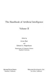
Preface This collection represents the primary reference work for researchers and students working in the area of Temporal Reasoning in Artificial Intelligence. As can be seen from the content, temporal reasoning has a vital role to play in many areas of Artificial Intelligence. Yet, until now, there has been no single volume collecting together the breadth of work in this area. This collection brings together the leading researchers in a range of relevant areas and provides an coherent description of the variety of activity concerning temporal reasoning within the field of Artificial Intelligence. To give readers an indication of what is to come, we provide an initial, simple example. By examining what options are available for modelling time in such an example, we can get a picture of the variety of topics related to temporal reasoning in Artificial Intelligence. Since many of these topics are covered within chapters in this Handbook, this also serves to give an introduction to the subsequent chapters. Consider the labelled graph represented in Figure 1:
Figure 1: Simple graph structure. This is a simple directed graph with nodes el and e2. The edge is labelled by a and P ( a ) and Q(b) represent some contents associated with the nodes. We can think of P and Q as predicates and a and b as individual elements. This can represent many things. The two nodes might represent physical positions, with the 'a' representing movement. Alternatively, el and e2 might represent alternate views of a systems, or mental states of an agent, or relationships. Thus this simple graph might characterise a wide range of situations. In general such a situation is a small part of a bigger structure described by a bigger graph. However, we have simply identified some typical components.
PREFACE
xii
Now add a temporal dimension to this, i.e., assume our graph varies over time. One can think of the graph as, for example, representing web pages, agent actions, or database updates. Thus, the notion of change over time is natural. The arrow simply represents an accessibility relation with a parameter a and with P ( a ) and Q ( b ) relating to node contents. As time proceeds, the contents may change, the accessibility relation may change; in fact, everything may change. Now, if we are to model the dynamic evolution of our graph structure, then there are a number of questions that must be answered. Answers to these will define our formal model and, as we will see below, the possible options available relate closely to the chapters within this collection. Question 1: Whatproperties of time do we need for our application? Formally, we might use (T,~(day, groups1 ( d a y ) ) ) ) ) ) y e a r = groupl2(month) a c a d e m i c y e a r = anchor select
-
group(day,
-
by - i n t e r s e c t i ( b u s i - d a y , select
-
downi(month)
As a matter of fact, these granularities can be generated in a more controlled way. Indeed, the authors distinguish three layers of granularities: L1 containing the bottom granularity and all the granularities obtained by applying group, alter, and s h i f t on granularities of this layer; L2 including L1 and containing all the granularities obtained by applying subset, union, intersection, and difference on granularities of this layer and selections with first
operand belonging to this layer; LB including L2 and containing all the granularities obtained by applying combine on granularities of this layer and anchor - group with the second operand on granularities
of this layer. Granularities of L 1 are full-integer labelled granularities, those of La may not be labelled by all integers, but they contain no gaps within granules. These aspects, as well as the expressiveness of the generated granularities, are investigated in depth in [Bettini et al., 20001.
3.3.5 Constraint solving and query answering Wang et al. [Wang et al., 19951 have proposed an extension of the relational data model which is able to handle granularity. The goal of this work is to take into account possible granularity mismatch in the context of federated databases. An extended temporal model is a relational database in which each tuple is timestamped under some granularity. Formally, it is a set of tables such that each table is a quadruple
J6r6me Euzenat & Angelo Montanari
74
( R ,4, T , g ) such that R is a set of tuples (a relational table), g is a granularity, 4 : N --+ 2 R maps granules to tuples, T : R 2N maps tuples to granules such that Vt E R, t E 4 ( i ) + i E ~ ( tand ) Vi E N,i E ~ ( t+) t E 4 ( i ) . In [Bettini et al., 20001, the authors develop methods for answering queries in database with granularities. The answers are computed with regard to hypotheses tied to the databases. These hypotheses allow the computation of values between two successive timestamps. The missing values can, for instance, be considered constant (persistence) or interpolated with a particular interpolation function. These hypotheses also apply to the computation of values between granularity. --+
The hypotheses (H)provide the way to compute the closure ( D H ) of a particular database (D). Answering a query q against a database with granularities D and hypotheses H consists in answering the query against the closure of the database (DH q). Instead of computing this costly closure, the authors proposes to reduce the database with regard to the hypotheses (i.e., to find the minimal database equivalent to the initial one modulo closure) and to add to the query formulas allowing the computation of the hypotheses. The authors also define quantitative temporal constraint satisfaction problems under granularity whose variables correspond to points and arcs are labelled by an integer interval and a granularity. A pair of points ( t ,t ' ) satisfies a constraint [m,n]g (with m,n E Z and g a granularity) if and only if r g t and f g t' are defined and m 5 1 r g t- f 9 t'l 5 n. These constraints cannot be expressed as a classical TCSP (see Chapter 7). As a matter of fact, if the constraint [0 0] is set on two entities under the hour granularity, two points satisfy it if they are in the same hour. In terms of seconds, the positions should differ from 0 to 3600. However, [0 36001 under the second granularity does not corresponds to the original constraint since it can be satisfied by two points in different hours. The satisfaction problem for granular constraint satisfaction is NP-hard (while STP is polynomial) [Bettini et al., 19961. Indeed the modulo operation involved in the conversions can introduce disjunctive constraints (or non convexity). For instance, next business day is the convex constraint ([I I]),which converted in hours can yield the constraint [l241 v [49 721 which is dependent on the exact day of the week. The authors propose an arc-consistency algorithm complete for consistency checking when the granularities are periodical with regard to some common finer granularity. They also propose an approximate (i.e., incomplete) algorithm by iterating the saturation of the networks of constraints expressed under the same granularity and then converting the new values into the other granularities. The work described above mainly concerns aligned systems of granularity (i.e., systems in which the upward conversion is always defined). This is not always the case, as the weeWmonth example illustrates it. Non-aligned granularity has been considered by several authors. Dyreson and collaborators [Dyreson and Snodgrass, 19941 define comparison operators across granularities and their semantics (this covers the extended comparators of [Wang et al., 19951): comparison between entities of different granularities can be considered under the coarser granularity (here coarser is the same as "groups into" above and thus requires alignment) or the finer one. They define upward and downward conversion operators across comparable granularities and the conversion across non-comparable granularities is carried out by first converting down to the greatest lower bound and then up (assuming the greatest lower bound exists and thus that the structure is a lower semi-lattice): L&, f $, x. Comparisons across granularities (with both semantics) are implemented in terms of the
+
I
3.3. THE SET-THEORETICAPPROACH conversion operators.
3.3.6 Alternative accounts of time granularity The set-theoretic approach has been recently revisited and extended in several directions. In the following, we briefly summarize the most promising ones. An alternative string-based model for time granularities has been proposed by Wijsen [Wijsen, 20001. It models (infinite) granularities as (infinite) words over an alphabet consisting of three symbols, namely, W (filler), 0 (gap), and [ (separator), which are respectively used to denote time points covered by some granule, to denote time points not covered by any granule, and to delimit granules. Wijsen focuses his attention on (infinite) periodical granularities, that is, granularities which are left bounded and, ultimately, periodically groups time points of the underlying temporal domain. Periodical granularities can be identified with ultimately periodic strings, and they can be finitely represented by specifying a (possibly empty) finite prefix and a finite repeating pattern. As an example, the granularity Businessweek W W W W W 0 0 1 W W W W W 0 0 1 . . . can be encoded by the empty prefix E and the repeating pattern W W W W B 0 0 1 . Wijsen shows how to use the string-based model to solve some fundamental problems about granularities, such as the equivalence problem (to establish whether or not two given representations define the same granularity) and the minimization problem (to compute the most compact representation of a granularity). In particular, he provides a straightforward solution to the equivalence problem that takes advantage of a suitable aligned form of strings. Such a form forces separators to occur immediately after an occurrence of W, thus guaranteeing a one-to-one correspondence between granularities and strings. The idea of viewing time granularities as ultimately periodic strings establishes a natural connection with the field of formal languages and automata. An automaton-based approach to time granularity has been proposed by Dal Lago and Montanari in [Dal Lago and Montanari, 20011, and later revisited by Bresolin et al. in [Bresolin et al., 2004; Dal Lago et al., 2003a; Dal Lago et al., 2003bl. The basic idea underlying such an approach is simple: we take an automaton A recognizing a single ultimately periodic word u E ( 0 , W , 4 ) " and we say that A represents the granularity G if and only if u represents G. The resulting framework views granularities as strings generated by a specific class of automata, called Single-String Automata (SSA), thus making it possible to (re)use well-known results from automata theory. In order to compactly encode the redundancies of the temporal structures, SSA are endowed with counters ranging over discrete finite domains (Extended SSA, ESSA for short). Properties of ESSA have been exploited to efficiently solve the equivalence and the granule conversion problems for single time granularities [Dal Lago et al., 2003bl. The relationships between ESSA and Calendar Algebra have been systematically investigated by Dal Lago et al. in [Dal Lago et al., 2003a1, where a number of algorithms that map Calendar Algebra expressions into automaton-based representations of time granularities are given. Such an encoding allows one to reduce problems about Calendar Algebra expressions to equivalent problems for ESSA. More generally, the operational flavor of ESSA suggests an alternative point of view on the role of automaton-based representations: besides a formalism for the direct specification of time granularities, automata can be viewed as a low-level formalism into which high-level time granularity specifications, such as those of Calendar Algebra, can be mapped. This allows one to exploit the benefits of both formalisms, using a high level language to define granularities and their properties in a natural and flexible
76
Jkr6me Euzenat & Angelo Montanan
way, and the automaton-based one to efficiently reason about them. Finally, a generalization of the automaton-based approach from single periodical granularities to (possibly infinite) sets of granularities has been proposed by Bresolin et al. in [Bresolin et al., 20041. To this end, they identify a proper subclass of Biichi automata, called Ultimately Periodic Automata (UPA), that captures regular sets consisting of only ultimately periodic words. UPA allow one to encode single granularities, (possibly infinite) sets of granularities which have the same repeating pattern and different prefixes, and sets of granularities characterized by a finite set of non-equivalent patterns, as well as any possible combination of them. The choice of Propositional Linear Temporal Logic (Propositional LTL) as a logical tool for granularity management has been recently advocated by Combi et al. in [Combi et al., 20041. Time granularities are defined as models of Propositional LTL formulas, where suitable propositional symbols are used to mark the endpoints of granules. In this way, a large set of regular granularities, such as, for instance, repeating patterns that can start at an arbitrary time point, can be captured. Moreover, problems like checking the consistency of a granularity specification or the equivalence of two granularity expressions can be solved in a uniform way by reducing them to the validity problem for Propositional LTL, which is known to be in PSPACE. An extension of Propositional LTL that replaces propositional variables by first-order formulas defining integer constraints, e.g., x = k y, has been proposed by Dernri in [Demri, 20041. The resulting logic, denoted by PLTL""~(P~S~ LTL with integer periodicity constraints), generalizes both the logical framework proposed by Combi et al. and the automaton-based approach of Dal Lago and Montanari, and it allows one to compactly define granularities as periodicity constraints. In particular, the author shows how to reduce the equivalence problem for ESSA to the model checking problem for PLTL'""~(-automata), which turns out to be in PSPACE, as in the case of Propositional LTL. The logical approach to time granularity is systematically analyzed in the next section, where various temporal logics for time granularity are presented.
3.4 The logical approach A first attempt at incorporating time granularity into a logical formalism is outlined in [Corsetti et al., 1991a; Corsetti et al., 1991bl. The proposed logical system for time granularity has two distinctive features. On the one hand, it extends the syntax of temporal logic to allow one to associate different granularities (temporal domains) with different subformulas of a given formula; on the other hand, it provides a set of translation rules to rewrite a subformula associated with a given granularity into a corresponding subformula associated with a finer granularity. In such a way, a model of a formula involving different granularities can be built by first translating everything to the finest granularity and then by interpreting the resulting (flat) formula in the standard way. A major problem with such a method is that there exists no a standard way to define the meaning of a formula when moving from a time granularity to another one. Thus, more information is needed from the user to drive the translation of the (sub)formulas. The main idea is that when we state that a predicate p holds at a given time point x belonging to the temporal domain T, we mean that p holds in a subset of the interval corresponding to x in Such a subset can be the whole interval, a scattered sequence of smaller the finer domain T'. intervals, or even a single time point. For instance, saying that "the light has been switched on at time x,,,", where x,i, belong to the domain of minutes, may correspond to state
3.4. THE LOGICAL APPROACH
77
that a predicate switching~nis true at the minute xmin and exactly at one second of xmin. Instead, saying that an employee works at the day xd generally means that there are several minutes, during the day xd, where the predicate work holds for the employee. These minutes are not necessarily contiguous. Thus, the logical system must provide the user with suitable tools that allow him to qualify the subset of time intervals of the finer temporal domain that correspond to the given time point of the coarser domain. A substantially different approach is proposed in [Ciapessoni et al., 1993; Montanari, 1994; Montanari, 19961, where Montanari et al. show how to extend syntax and semantics of temporal logic to cope with metric temporal properties possibly expressed at different time granularities. The resulting metric and layered temporal logic is described in detail in Subsection 3.4.1. Its distinctive feature is the coexistence of three different operators: a contextual operator, to associate different granularities with different (sub)formulas, a displacement operator, to move within a given granularity, and a projection operator, to move across granularities. An alternative logical framework for time granularity has been developed in the classical logic setting [Montanari, 1996; Montanari and Policriti, 1996; Montanari et al., 19991. It imposes suitable restrictions to languages and structures for time granularity to get decidability. From a technical point of view, it defines various theories of time granularity as suitable extensions of monadic second-order theories of k successors, with k 1. Monadic theories of time granularity are the subject of Subsection 3.4.2. The temporal logic counterparts of the monadic theories of time granularity, called temporalized logics, are briefly presented in Subsection 3.4.3. This way back from the classical logic setting to the temporal logic one passes through an original class of automata, called temporalized automata. A coda about the relationships between logics for time granularity and interval temporal logics concludes the section.
>
3.4.1 A metric and layered temporal logic for time granularity Original metric and layered temporal logics for time granularity have been proposed by Montanari et al. in [Ciapessoni et al., 1993; Montanari, 1994; Montanari, 19961. We introduce these logics in two steps. First, we take into consideration their purely metric fragments in isolation. To do that, we adopt the general two-sorted framework proposed in [Montanari, 1996; Montanari and de Rijke, 19971, where a number of metric temporal logics, having a different expressive power, are defined as suitable combinations of a temporal component and an algebraic one. Successively, we show how flat metric temporal logic can be generalized to a many-layer metric temporal logic, embedding the notion of time granularity [Montanari, 1994; Montanari, 19961. We first identify the main functionalities a logic for time granularity must support and the constraints it must satisfy; then, we axiomatically define metric and layered temporal logic, viewed as the combination of a number of differently-grained (single-layer) metric temporal logics, and we briefly discuss its logical properties. The basic metric component The idea of a logic of positions (topological, or metric, logic) was originally formulated by Rescher and Garson [Rescher and Garson, 1968; Rescher and Urquhart, 19711. In [Rescher
JLr6me Euzenat & Angelo Montanan'
78
and Garson, 19681, the authors define the basic features of the logic and they show how to give it a temporal interpretation. Roughly speaking, metric (temporal) logic extends propositional logic with a parameterized operator A, of positional realization that allows one to constrain the truth value of a proposition at position a. If we interpret the parameter a as a displacement with respect to the current position, which is left implicit, we have that A,q is true at a position x if and only if q is true at a position y at distance a from x. Metric temporal logics can thus be viewed as two-sorted logics having both formulas and parameters; formulas are evaluated at time points while parameters take values in a suitable algebraic structure of temporal displacements. In [Montanari and de Rijke, 19971, Montanari and de Rijke start with a very basic system of metric temporal logic, and they build on it by adding axioms andlor by enriching the underlying structures. In the following, we describe the metric temporal logic of two-sorted frames with a linear temporal order (MTL); we also briefly consider general metric temporal logics allowing quantification over algebraic and temporal variables and free mixing of algebraic and temporal formulas (Q-MTL). The two-sorted temporal language for MTL has two components: the algebraic component and the temporal one. Given a non-empty set A of constants, let T ( A )be the set of terms over A, that is, the smallest set such that A T ( A ) and , if a, P E T ( A )then a + p, -a, 0 E T ( A ) .The first-order (algebraic) component is built up from T ( A )and the predicate symbols = and (REP) where ( $ 1 ~ )denotes substitution of 4 for the variable p; (transfer of identities). (LIFT) t a = P ==+ k V a 4 tt V p 4 +-+
+
Axiom (AxN) is the usual distribution axiom; axiom (AxS) expresses that a displacement a is the converse of a displacement - a ; axioms (AxR), (AxT), and (AxQ) capture reflexivity, transitivity, and quasi-functionality with respect to the third argument, respectively. A suitable adaptation of two truth preserving constructions from standard modal logic to the MTL setting allows one to show there are no MTL formulas that express total connectedness and quasi-functionality with respect to the second argument of the displacement relation [Montanari and de Rijke, 19971. The rules (D-NEC) and (REP) are familiar from modal logic. Finally, the rule (LIFT) allows one to transfer provable algebraic identities from the displacement domain to the temporal one. A derivation in MTL is a sequence of formulas al,. . . , a, such that each ai,with 1 5 i, 5 n, is either an axiom or obtained from 01, . . . , a,-1 by applying one of the derivation a to denote that there is a derivation in MTL that ends in a. rules of MTL. We write kMTL It immediately follows that tMTL a = ,B iff a = P is provable from the axioms of the algebraic component only: whereas we can lift algebraic information from the displacement domain to the temporal domain using the (LIFT) rule, there is no way in which we can import temporal information into the displacement domain. As with consequences, we only consider one-sorted inferences 'Tt 4'.
Theorem 3.4.1. MTL is sound and completefor the class of all transitive, rejexive, totallyconnected, and quasi,functional (in both the second and third argument of their displacement relation) frames.
3.4. THE LOGICALAPPROACH
81
The proof of soundness is trivial. The completeness proof is much more involved [Montanari and de Rijke, 19971. It is accomplished in two steps: first, one proves completeness with respect to totally connected frames via same sort of generated submodel construction; then, a second construction is needed to guarantee quasi-functionality with respect to the second argument. Propositional variants of MTL are studied in [Montanari and de Rijke, 19971. As an example, one natural specialization of MTL is obtained by adding discreteness. As in the case of the ordering, the discreteness of the temporal domain necessarily follows from that of the domain of temporal displacements, which is expressed by the following formula:
Proposition 3.4.1. Let F = (T, D;DIS)be a two-sorted frame based on a discrete ordered Abelian group D. For all i, j 6 T,there exist onlyjnitely many k such that i
>
*This actually presents an alternative way to define the semantics of the fixed point formulae in the case that the function f is monotone.
158
Howard Barringer & Dov Gabbay
and never gets removed by the iteration. On the other hand, the construction of the minimal solution to f starts from the empty set and adds all models satisfying the property that q is true at some future point and p is true up to that point. The model with p true everywhere (from i ) and q never true (from i onwards) is never added. The minimal fixed point formula thus corresponds to p until q and the maximal fixed point formula is the weak version, namely p W q. The examples we've shown so far have no nesting of fixed points. However, our language allows such formulae. Suppose therefore that f ( x ,y ) is monotone in both variables x and y; it can be shown that if x
+ x' then uy.f ( x ,y) * v y . f( x ' ,y)
It follows that a general condition for monotonicity of f ( x ) is that x must occur under an even number of negations. If this is the case for all bound variables of a fixed point formula, then the fixed point does exist. For example, v x .( a A Ow y . ( ~ x AyO) )is defined, x appears under two negations, the innermost being applied direct to x , then another encompassing negation applied to the immediately surrounding v formula. The use of negation applied to bound variables, in such cases, can be avoided by the use of minimal fixed point formulae. The example just given can be rewritten as v x . ( a A O,uy.(x V 0 y ) ) . Indeed, if a formula f has no negation symbols applied to bound variables, then the formula f can also be written without negation applied to bound variables. 7
Decidability The propositional temporal fixed point logic, uTL, over linear discrete frames (W, I 1 . Let P = {u(UTER f ( ~ 1 I 1(21,~ R, W ) E E l . if PAsAT(P) then accept else reject
Algorithm 6.4.4. ( ~ l g - v - S A T ( v ; ~ ) ) input Instance G 1 2 3 4
=
(V, E ) of V-SAT(V;')
if G contains Ithen reject else accept
0
6.5 Formalisms with Metric Time We will now examine known tractable formalisms allowing for metric time, and which are not subsumed by the Horn-DLR framework. By formalisms allowing metric time, we mean formalisms with the ability to express statements such as "X happened at time point 100" or "X happened at least 50 time units before Y". Note that Allen's algebra cannot express this, while the Horn DLRs can. The first example is an extension to the continuous endpoint formulae, and the second is a method for expressing metric time in the sub-algebras S(.),E ( . ) ,S*and E*.
6.5.1 Definitions Definition 6.5.1. (Augmented (continuous) endpoint formula) An augmented (continuous) endpoint formula [Meiri, 19961 is 1. a (continuous) point algebra formula; or 2. a formula of the type z E {[d;, d t ] , . . . , [d;, d:]), whered; , . . . , d;,dt,d; ~ Q a n d d ;
--
+ >
+
>
>
>
7.4. THE? SCHEME OF INDEFINITE CONSTRAINTDATABASES
23 1
In this example the set of rationals Q is our time line. The year 1996 is assumed to start at time 0 and every interval [i,i + 1 ) represents a day (for i E 2 and i 2 0). Time intervals will be represented by their endpoints. They will always be assumed to be of the form [ B ,E ) where B and E are the endpoints. The above database represents the following information: 1. There are three scheduled appointments for treatment of patient Smith. This is represented by three conjuncts within the disjunction dejining the extension of the predicate treatment. 2. Chemotherapy appointments must be scheduled for a single day. Radiation appointments must be scheduled for two consecutive days. This information is represented by constraints w2 = wl 1 , w4 = w3 1 , and ws = ws + 2.
+
+
3. The first chemotherapy appointment for Smith should take place in the jirst three months of 1996 (i.e., days 0-91). This information is represented by the constraints wl 2 0 and w2 5 91. 4. The second chemotherapy appointment for Smith should take place in the second three months of 1996 (i.e., days 92-182). This information is represented by constraints w3 91 and w4 5 182.
>
5. Thejirst chemotherapy appointment for Smith must precede the second by at least two months (60 days). This information is represented by constraint w3 - w2 2 60.
6. The radiation appointment for Smith should follow the second chemotherapy appointment by at least 20 days. Also, it should take place before the end of July (i.e., day 213). This information is represented by constraints ws - w4 2 20 and ws 5 213. Let us now define queries. The concept of query defined here is more expressive than the query languages for temporal constraint networks proposed in [Brusoni et al., 1994; Brusoni et al., 1997; van Beek, 19911, and it is similar to the concept of query in TMM [Schrag et al.. 19921.
Definition 7.4.2. A first order modal query over an indejinite constraint database is an expression of the form Z / D , t/? : O P +(%, t ) where OP is the modal operator 0 or 0, and 4 is a formula of (C U EQ)*. The constraints in formula 4 are only C constraints and & Q constraints. Modal queries will be distinguished in certainty or necessity queries (0) and possibility queries (0).
Example 7.4.4. Thefollowing query refers to the database of Example 7.4.2 and asks "Who was the person who possibly had a conversation with Fred during this person's walk in the park?":
x / D : 0 ( 3 t i ,t2, t s , t 4 / & ) ( w a l k ( x ,t l , t2) A talk(%,Fred, t 3 ,t4) A t l < t 3 A t4 < t 2 )
232
Manolis Koubarakis
Let us observe that each query can only have one modal operator which should be placed in front of a formula of (C u &&)*. Thus we do not have a full-fledged modal query language like the ones in [Levesque, 1984; Lipski, 1979; Reiter, 19881. Such a query language can be beneficial in any application involving indefinite information but we will not consider this issue in this chapter. We now define the concept of an answer to a query.
Definition 7.4.3. Let q be the query Z/D,T/T : o$@, i) over an indejnite constraint database D B . The answer to q is apair (answer(:, f), 0)such that I. answer(^, i) is a formula of the form
where Local, (Z, i) is a conjunction of L constraints in variables 2and EQ constraints in variables.
2. Let V be a variable assignment for variables Z and i. If there exists a model M of D B which agrees with M L u E eon the interpretation of the symbols of C U EQ, and M satisjes @, i) under V then V satisfies answer(:, 8and vice versa. We have chosen the notation (answer(3l,i), 0) to signify that an answer is also a database which consists of a single predicate defined by the formula answer(?E, i?) and the empty constraint store. In other words, no Skolem constant (i.e., no uncertainty) is present in the answer to a modal query. Although our databases may contain uncertainty, we know for sure what is possible and what is certain.
Example 7.4.5. The answer to the query of Example 7.4.4 is (x = M a r y ,
0).
The definition of answer in the case of certainty queries is the same as Definition 7.4.3 with the second condition changed to:
on the interpretation of the 2. Let M be any model of D B which agrees with M L u E Q symbols of C U &&. Let V be a variable assignment for variables Z and i?. I f M satisjies $(Z, 2) under V then V satisfies answer(??,t )and vice versa. Definition 7.4.4. A query is called closed or yeslno f i t does not have any free variables. Queries withfree variables are called open. Example 7.4.6. The query of Example 7.4.4 is open. The following is its corresponding closed query:
By convention, when a query is closed, its answer can be either (true, 0)(which means yes) or (false, 0) (which means no).
Example 7.4.7. The answer to the query of Example 7.4.6 is (true, 0) i.e., yes.
7.4. THE SCHEME OF INDEFINITE CONSTRAINTDATABASES
233
Let us now give some more examples of queries.
Example 7.4.8. Let us consider the database of Example 7.4.3 and the query "Find all appointments for patients that can possibly start at the 92th day of 1996". This query can be expressed as follows: The answer to this query is the following:
( (x = Smith A y
=
Chem2)V ( x = Smith A y
=
Radiation), true )
Example 7.4.9. Thefollowing query refers to the database of Example 7.4.3 and asks "Is it certain that thejrst Chemotherapy appointment for Smith is scheduled to take place in the jrst month of 1996?": : 0 ( 3 t l ,ta/Q)(treatment(Smith,Cheml,t l ,t 2 )A 0
5 t l < t 2 < 31)
The answer to this query is no.
7.4.3 Query Evaluation is Quantifier Elimination Query evaluation over indefinite constraint databases can be viewed as quantifier elimination ) quantifier elimination. This is a consein the theory T h ( M L U s Q )T. h ( M L u E Qadmits quence of the assumption that T h ( M L admits ) quantifier elimination (see beginning of this section) and the fact that T ~ ( M admits E ~ ) quantifier elimination (proved in [Kanellakis et al., 19951). The following theorem is essentially from [Koubarakis, 1997b1.
Theorem 7.4.1. Let DB be the indefinite constraint database
and q be the query y/D, : O4(y,2). The answer to q is (answer@,F), 0) where answer@, Z ) is a disjunction of conjunctions of E Q constraints in variables ?j and C constraints in variables 2 obtained by eliminating quantijiers from the following formula of C=:
In this formula the vector of Skolem constants C has been substituted by a vector of appropriately quantijied variables with the same name (?? is a vector of sorts of C). $ ( y ,%, SLi) is obtained from 4 ( y ,Z ) by substituting every atomic formula with database predicate pi by an equivalent disjunction of conjunctions of C constraints. This equivalent disjunction is obtained by consulting the definition 1%
V Localj (%,t,,J ) = p, ( K ,5)
j=1
of predicate pi in the database DB.
234
Manolis Koubarakis
I f q is a certainty query then answer(y,F ) is obtained by eliminating quantiJiers from the formula
where ConstraintStore(9) and
$(y, 2, i;~)are defined as above.
Example 7.4.10. Using the above theorem, the query of Example 7.4.4 can be answered by eliminating quantiJiers from the formula:
( 3 w l , w 2 , ~w 3 ,d Q ) (wl < w 2 A w l <wg Awg<w2Aw3 <w4A ( 3 t l ,t 2 ,t 3 ,t 4 / & ) ( ( x= Mary A t l = wl A t 2 = w2)A (x = Mary A t3 = w3 A tq = w4)A t l < t3 A t4 < t 2 ) The result of this elimination is the formula x
=
Mary.
Answering queries by the above method is mostly of theoretical interest. For implementations of this scheme more efficient alternatives have to be considered. Let us close this section by pointing out that what we have defined is a database scheme. Given various choices for C (e.g., C = L I N ) , one gets a model of indefinite constraint databases (e.g., the model of indefinite L I N constraint databases). Examples of such instantiations will be seen repeatedly in the forthcoming Sections 7.5, 7.6 and 7.7 where we demonstrate that the proposals of [van Beek, 1991; Brusoni et al., 1994; Brusoni et al., 1995b; Brusoni et al., 1997; Brusoni et al., 1995a; Brusoni et al., 1999; Koubarakis, 1993; Koubarakis, 1994b1 are subsumed by the scheme of indefinite constraint databases.
7.5 The LATERSystem In [Brusoni et al., 1994; Brusoni et al., 1997; Brusoni et al., 1995b1 sets of L A T E Rconstraints are considered as knowledge bases with indefinite temporal knowledge, and are queried in sophisticated ways using a first-order modal query language. This section will show that query answering in the LATER system is really an instance of the scheme of indefinite constraint databases. We will first specify a method for translating a LATER knowledge base K B (i.e., a set of L A T E Rconstraints) to an indejinite L A T E Rconstraint database D B . The translation is done in two steps. First, for each symbolic point or interval I in K B , we introduce a fact happensI ( w I )in EventsAndFacts(DB) where happensr is a new database predicate and wI is a new Skolem constant of appropriate sort. Then, for each constraint c between symbolic intervals I and J in K B , we introduce the same constraint between Skolem constants wl and W J in ConstraintStore(DB). Example 7.5.1. The following is the indejinite L A T E R constraint database which corresponds to the LATER knowledge base of Example 7.2.4.*
'In this and the next section we do not follow Definition 7.4.1 precisely for reasons of clarity and prefer to write sets of conjuncts instead of conjunctions. Also, when it comes to EventsAndFacts(DB),we write positive atomic formulas of first order logic and mean the completions of these formulas [Reiter, 19841.
7.5. THE LATER SYSTEM h a ~ ~ e n ~ ~ n n ~ o r k ( ~ ), ~ n n ~ o r k )
{W
T
~
Since ~ W 1/1/1995 ~ ~ 14~: 15,
W T ~ ~ W B O eTf o~r e W
M
~
~ W~
start(wAn,woTk)At 1/1/1995,
W
W
T
~
Until ~ W 1/1/1995 ~ ~ 18 ~: 30,
W M
~ ~ ~Lasting ~ ~ ~,
A
~
AtW Least ~ 4~ : 40~ hours,
Lasting ~ W 3 ~: 00~hours, ~
end(wAnnwoTk) B e f o r e 1/1/1995 18 : 00 ) ) Now it is easy to translate queries over a LATERknowledge base to first order modal queries over an indefinite L A T E R constraint database. We will consider all types of queries presented in [Brusoni et al., 1994; Brusoni et al., 1995b; Brusoni et al., 19971. 1. WHEN queries. A WHEN query is of the form
WHEN T? where T is a symbolic point or interval in the queried LATERknowledge base. For the case of intervals, the corresponding query in our framework is
and similarly for points.
Example 7.5.2. The query W H E NTomWork ? is translated into : ha~~en~Tom~ork(~)
and has the following answer over the database of Example 7.2.4:
{ W T o m W o r k Since 1/1/1995 14 : 15,
W
T
~
Until ~ W 1/1/1995 ~ ~ 18 ~: 30 ) )
2. MUST queries. A MUST query in its simplest form is
m u s t c ( I ,J ) ? where I , J are symbolic time intervals and c is a temporal constraint in LATER (similarly for points). The corresponding query in our framework is : ~ ( 3 2y /, Z ) ( h a p p e n s r ( x )A ~ ~ P P ~ ~ sAJ c(( xY,Y) ) )
The extension to arbitrary MUST queries is straightforward.
Manolis Koubarakis Example 7.5.3. The query
M U S T overlaps(AnnWork,M a r y W o r k ) ? can be translated into :
(334y / T ) ( h a p p e n s ~ , , ~ ~ ,(kx )A h a ~ ~ e n s ~ ~ ~ ,AwOuerlaps(z, ~ ~ k ( y )Y ) )
The answer to this query over the LATERKB of Example 7.2.4 is
which means NO.
3. MAY queries. The translation is similar to MUST queries but now the modal operator 0 is used. 4. Hypothetical queries. The query language of our framework does not support hypothetical queries. They can be simulated by updating the database with an appropriate set of constraints and then asking a query.
7.6 Van Beek's Proposal for Querying IA Networks In [van Beek, 19911 van Beek went beyond the typical reasoning problems studied for IA networks and considered them as knowledge bases about events that can be queried in more sophisticated ways. This section will show that van Beek's efforts can also be subsumed by our framework. In [van Beek, 19911 an IA knowledge base is a set of Interval Algebra constraints among appropriately named event constants (see Example 7.2.2). We will first specify a method for translating an IA knowledge base K B to an indefinite I A constraint database D B . The translation is done in two steps. First, for each event e in K B , we introduce the facts
in E v e n t s A n d F a c t s ( D B )where event and happens are database predicates and w e is a new Skolem constant of sort T.* Then, for each constraint c between events el and ez in K B , we introduce the same constraint between events we, and we, in ConstraintStore(DB). Example 7.6.1. Thefollowing is the indejinite I A constraint database corresponding to the I A constraints of Example 7.2.2:
( { event(break f a s t ) , event(paper), event(cof f ee), event(walk),
*Let Z be the only sort of language I A
7.6. VANBEEK'S PROPOSAL FOR QUERYINGIA NETWORKS
TheJirst component of the above pair asserts the existence offour events and their times. The second component asserts "all we know" about these times in the form of I A constraints.
It is easy to translate queries over an IA KB to first order modal queries over an indefinite I A constraint database. We will consider all types of queries presented in [van Beek, 19911. 1. Possibility and certainty queries. These are very similar to MAY and MUST queries in LATER.The translation to our framework is also very similar. A certainty (resp. possibility) query is a formula of the form
where O P is (resp. o),and 4 is a quantifier free formula of I A with free variables e l , . . . , en. In our framework the corresponding query is
2. Aggregation questions. An aggregation question is of the form
where E is the set of all events in the KB, OP is the modal operator 0 or a quantifier free first order formula of IA.
and 4 is
The corresponding query in our framework is
Example 7.6.2. Thefollowing IA KB provides information about a patient's visits to the hospital during the period 1990-1991: 1990 meets 1991, visit4 during 1990, visit5 during 1990,
Manolis Koubarakis visit6 during 1991, visit7 during 1991, visit4 before visit5, visit5 before visit6, visit6 before visit7 The aggregation query x : x E V i s i t s A ~ ( during x 1991) where V i s i t s is the set of all events can be translated into the following query in our framework: ) h a p p e n s ( x , t )A O ( X during 1991)) x / V : ( 3 t / Z ) ( e v e n t ( xA Note that calendars are not part of I A . To deal with them we follow our approach for L A T E R : calendar primitives (e.g., years) can be introduced as terms of the language and interpreted accordingly. l f t h e above query is executed over the indejinite I A constraint database which corresponds to KB (it is easy to construct this database as it was done in Example 7.6.1) then it has the following answer: ( { x = v i s i t l , x = uisit7), 0)
7.7 Other Proposals In [Brusoni et al., 1995a; Brusoni et al., 19991 the LATER team extended the relational model of data with the temporal reasoning facilities of LATER.In their proposal, a relational database stores non-temporal information about events and facts which times are constrained by a set of L A T E Rconstraints. Earlier (and independently) similar work had been done by Koubarakis in [Koubarakis, 1993; Koubarakis, 1994b1 where the model of indefinite temporal constraint databases was first defined as an extension of the relational data model. The above data models and query languages are instantiations of the scheme of indefinite constraint databases presented in this chapter. The model of [Brusoni et al., 1995a; Brusoni et al., 19991 is essentially the model of indejinite L A T E R constraint databases. Similarly the model of [Koubarakis, 1993; Koubarakis, 1994b1 is the model of indejinite D I F F constraint databases. The only notable difference is that in this chapter we have developed our framework using first-order logic while Koubarakis, Brusoni, Console, Pernici and Terenziani use the relational data model. Another related effort is of course TMM [Dean and McDermott, 1987; Schrag et al., 19921 that can be seen to be an ancestor of all of the above systems. TMM has a very expressive representation language so it cannot be presented under the umbrella of the proposed scheme. However, if we omit persistence assumptions, projection rules and dependencies from the TMM formalism then the resulting subset is subsumed by indefinite D I F F constraint databases. Now that we have investigated the representational power of the indefinite constraint database scheme in detail, we turn to its computational properties and ask the following
7.8. QUERY ANSWERINGIN INDEFINIE CONSTRAINTDATABASES
239
question: What is the computational complexity of the proposed scheme when constraints encode temporal information? In particular, do we stay within PTIME when the classes of constraints utilised for representing temporal information have satisfiability and variable elimination problems that can be solved in PTIME? These questions are answered in the following section.
7.8 Query Answering in Indefinite Constraint Databases In this section, we study the computational complexity of evaluating possibility and certainty queries over indefinite constraint databases when constraints belong to the temporal languages studied in Section 7.2. The complexity of query evaluation will be measured using the notion of data complexity originally introduced by database theoreticians [Vardi, 19821. When we use data complexity, we measure the complexity of query evaluation as a function of the database size only; the size of the query is consideredfixed. This assumption is reasonable and it has also been made in previous work on querying temporal constraint networks [van Beek, 19911. For the purposes of this chapter the size of the database under the data complexity measure can be defined as the number of symbols of a binary alphabet that are used for its encoding. We already know that evaluating possibility queries over indefinite constraint databases can be NP-hard even when we only have equality and inequality constraints between atomic values [Abiteboul et al., 19911; similarly evaluating certainty queries is co-NP-hard. It is therefore important to seek tractable instances of query evaluation.; The rest of this chapter does not consider equality constraints (from language &Q) as they have been used in the definition of databases (Definition 7.4.1) and queries (Definition 7.4.2). This can be done without loss of generality because they do not change our results in any way. We reach tractable cases of query evaluation by restricting the classes of C constraints, databases and queries we allow. The concepts of query type and database type introduced below allow us to make these distinctions.
7.8.1 Query Types A query type is a tuple of the following form: Q(OpenOrClosed, Modality, FO-Formula-Type, Constraints) The first argument of a query type can take the values Open or Closed and distinguishes between open and closed queries. The argument Modality can be 0 or representing possibility or necessity queries respectively. The third argument FO-Formula-Type can take the values FirstOrder, PositiveExistential or SinglePredicate. The value FirstOrder denotes that the first-order expression part of the query can be an arbitrary first-order formula. Similarly, PositiveExistential denotes that the first order part of the query is a positive existential formula i.e., it is of the form ( 3 ~ / ~ ) 4 where (5) 4 involves only the logical symbols A and V. Finally, SinglePredicate denotes that the query ~ where ( u , E and are vectors of variables, sl, S2 are is of the form u/sl : O P ( 3 i / ~ ~ ) i) vectors of sorts, p is a database predicate symbol and O P is a modal operator.
240
Manolis Koubarakis
The fourth argument Constraints denotes the class of constraints that are used in the query. Definition 7.4.2 allows queries to contain any constraint from the class of L constraints. This section will also consider restricting query constraints to members of any constraint class C such that C is a subclass of the class of C constraints.
7.8.2 Database Types A database type is a tuple of the following form:
D B ( A r i t y ,LocalCondition, ConstraintStore) Argument Arity denotes the maximum arity of the database predicates. It can take values
Monadic, Binary, T e r n a r y , . . . , N-ary (i.e., arbitrary). Argument LocalCondition denotes the constraint class used in the definition of the database predicates. Finally, argument ConstraintStore denotes the class of constraints in the constraint store. Definition 7.4.1 allows the local conditions and the constraint store to contain any constraint from the class of L constraints. This section will also consider restrictions to members of any constraint class C such that C is a subclass of the class of C constraints.
7.8.3 Constraint Classes In the rest of this section we will refer to certain constraint classes which we summarize below for ease of reference. Some of these classes have already been introduced in Section 7.2. Others are defined for the first time. 0
H D L , L I N , I A , S I A , ORD-Horn, P A and C P A defined earlier.
0
U T V P I and U T V P I ~ . A U T V P I constraint is a L I N constraint of the form rtxl
+
-- c or fxl x2 -- c where X I , 2 2 are variables ranging over the rational numbers, c is a rational constant and is 5. The class of U T V P I ~is obtained when is also allowed to be #.
-
-
The following are some examples of U T V P I ~constraints:
U T V P I constraints are a natural extension of D I F F constraints studied in [Dechter et al., 19891. They are also a subclass of T V P I constraints [Shostak, 1981; Jaffar et al., 19941. T V P I is an acronym for linear inequalities with at most Two Variables Per Inequality. In a similar spirit, U T V P I is an acronym for T V P I constraints with Unit coefficients. The class of U T V P I * constraints was first studied in [Koubarakis and Skiadopoulos, 1999; Koubarakis and Skiadopoulos, 20001.
2d-IA and 2d-ORD-Horn. The class 2d-IA is a generalization of I A in two dimensions and it is based on the concept of rectangle in Q2 [Guesgen, 1989; Papadias et al., 1995; Balbiani et al.,
7.8. QUERY ANSWERINGIN INDEFINITE CONSTRAINTDATABASES
24 1
19981. Every rectangle r can be defined by a Ctuple (LT,,L i , U,T,U T )that gives the . relations coordinates of the lower left and upper right comer of r. There are 133 basic in 2d-IA describing all possible configurations of 2 rectangles in Q 2 .
2d-ORD-Horn is the subclass of 2d-IA which includes only these relations R with the property
where
- 4 is a conjunction of ORD-Horn constraints on variables LT, and U,'. - II, is a conjunction of ORD-Horn constraints on variables L', and U,'. The above classes of constraints refer to spatial objects. It is interesting to consider them in this section because some interesting results for these can easily be obtained by the corresponding results for the temporal classes.
L I N E Q . This is the subclass of L I N which contains only linear equalities. 0
0
0
SORD. This is the sub-algebra of P A which contains only the relations {). In other words, SORD is the class of strict order constraints. W O R D .This is the sub-algebra of P A which contains only the relations ( 5 , 2).In other words, W O R Dis the class of weak order constraints. ORD-CON. This is the subclass of LIN which contains only constraints of the form x r where x is a variable, r is a rational constant and is , 5 , or 2 . N
0
0
0
UTVPI-EQ. This is the subclass of U T V P I which contains only equality constraints. RAT-EQUAL.This is the subclass of L I N E Q which contains only equality constraints of the form x = v where x is a variable and v is a variable or a rational constant (ordinary or Skolem). RAT-EQUAL-CON.This is the subclass of RAT-EQUALwhich contains only equality constraints of the form x = a where x is a variable and a is a rational constant (ordinary or Skolem). Among other things, this class is useful for specifying databases of type
D B ( A ,RAT-EQUAL-CON,C ) where A is an arity and C is a constraint class. In databases of this type, predicates are defined by completions (in the sense of [Reiter, 19841) of formulas of the formp(E, Z) where is a vector of rational constants and iiJ is a vector of Skolem constants. For example, the database
Manolis Koubarakis is of type
DB(3-ary, RAT-EQUAL-CON,S O R D ) These databases are typical of the kind of databases encountered in temporal and spatial problems involving indefinite information (where information about non-temporal entities like Mary and Fred of Example 7.4.2 has been abstracted away).
N O N E . This is the class which contains only the trivial constraints true and false. This class is useful for specifying queries with database predicates but no constraints. Also, it is useful for specifying databases of the form
where ConstraintStore(DB) = know nothing about them).
0 (i.e., there might be
Skolem constants but we
Now that we have introduced the constraints classes that we will consider, we are ready to present our results. Proofs are omitted and can be found in [Koubarakis and Skiadopoulos, 20001.
7.8.4
PTIME Problems
The following theorem gives our main PTIME upper bound.
Theorem 7.8.1. The evaluation of ( a ) Q(Closed,0, PositiveExistential, H D L ) queries over D B ( N - a r y ,H D L , H D L ) databases, ( b ) Q(Closed,O,PositiveExistential, L I N E Q ) queries over D B ( N - a r y ,L I N E Q , H D L ) databases,
(c) Q(Open,0, PositiveExistential, U T V P I f )queries over D B ( N - a r y ,U T V P I Z , U T V P I f )databases and ( d ) Q(Open,O , SinglePredzcate, N O N E ) queries over D B ( N - a r y ,U T V P I - E Q u U T V P -I ~ U , , T V P I Z )databases can be performed in PTIME. The above theorem is very interesting. It shows how classes with tractable satisfiability andlor variable elimination problems can be combined with a logical database framework to obtain a much more expressive representational framework where query answering still remains tractable. The reader should notice the restrictions on the queries and databases that enable tractability. Let us now consider databases and queries involving higher-order objects i.e., intervals and rectangles and derive a similar result.
Theorem 7.8.2. The evaluation of
7.8. QUERY ANSWERINGIN INDEFINITE CONSTRAINTDATABASES
243
( a ) Q(Closed,0, PositiveExistential, ORD-Horn) queries over DB(N-ary,ORD-Horn,ORD-Horn) databases, ( b ) Q(Closed,0, PositiveExistential, 2d-ORD-Horn) queries over D B ( N - a r y ,2d-ORD-Horn,2d-ORD-Horn) databases, ( c ) Q(Open, 0, PositiveExistential, S I A )queries over D B ( N - a r y ,S I A ,S I A )databases can be performed in PTIME.
Theorem 7.8.2(b) is an interesting result for rectangle databases with indefinite information over Q 2 . This result can be generalized to Qn if one defines an appropriate algebra nd-ORD-Horn.
7.8.5
Lower Bounds
The theorems of the previous section gave us restrictions on queries, databases and constraint classes that enable us to have tractable query answering problems. We now consider identifying the precise boundary between tractable and intractable query answering problems for indefinite constraint databases with linear constraints. We start our inquiry by considering whether the results of Theorem 7.8.1 can be extended to more expressive classes of queries. * For example, can we allow negation in the queries (equivalently, can we allow arbitrary first order formulas) and still get results like Theorem 7.8.l(a) or 7.8.l(b)? The following theorem shows that the answer to this question is negative.+ Theorem 7.8.3 ([Abiteboul et al., 19911). Let D B C be the set of databases of type
DB(4-ary, RAT-EQUAL-CON,N O N E ) with the additional restriction that every Skolem constant occurs at most once in any member of DBC. Then: 1. There exists a query q E Q(Closed, 0, FirstOrder, R A T - E Q U A L )such that deciding whether q(db) = yes is NP-complete even when db ranges over databases in the set DBC.
2. There exists a query q E Q(Closed, 0, FirstOrder, R A T - E Q U A L )such that deciding whether q(db) = yes is co-NP-complete even when db ranges over databases in the set DBC.
Theorem 7.8.l(a) and (b) together with the above theorem establish a clear separation between tractable and possibly intractable query answering problems. The presence of negation in the query language can easily lead us to computationally hard query evaluation problems (NP-complete or co-NP-complete) even with very simple input databases. Another issue that we would like to consider is whether one can improve Theorem 7.8.l(b) with a class which is more expressive than L I N E Q (for example L I N ) . The following result shows that this is not possible; even the presence of strict order constraints in the query is enough to lead us away from PTIME. "Similar issues arise for Theorem 7.8.2. The results of this section can easily be generalised to this case. t ~ h theorem e has been proved in [Abiteboul er ul., 19911 for equality constraints over any countably infinite domain thus it holds for the domain of rational numbers too.
Manolis Koubarakis
Theorem 7.8.4 ([van der Meyden, 19921). There exists a query in Q(Closed, 0 ,Conjunctive,S O R D ) with co-NP-hard data complexityover D B ( B i n a r y ,R A T - E Q U A L - C O NS, O R D ) databases. Note that for the above theorem to be true, S O R D constraints must be present both in the database and in the query. Otherwise, as Theorems 7.8.5 and 7.8.6 imply, conjunctive query evaluation can be done in PTIME.
Theorem 7.8.5. Evaluating Q(Closed, 0 ,PositiveExistential, N O N E ) queries over D B ( N - a r y ,R A T - E Q U A L - C O NH , DL) databases can be done in PTIME. Theorem 7.8.6. Evaluating Q(Closed,0 ,Conjunctive,L I N ) queries over D B ( N - a r y ,R A T - E Q U A L - C O N N , ONE) databases can be done in PTIME.
A final issue that the careful reader might be wondering about is whether Parts (c) and (d) of Theorem 7.8.1 can be extended. Let us consider Part (c) first. Theorem 7.8.3 shows that we should not expect to stay within PTIME if we move away from positive existential queries. So the only way that this result could be improved is by discovering a class C such that U T V P I ~c C c H D L and V A R - E L I M ( C is ) in PTIME. This is therefore an interesting open problem; its solution will also be very interesting to linear programming researchers [Hochbaum and Naor, 1994; Goldin, 19971. Let us now consider whether we can improve Theorem 7.8.l(d). The following result shows that this is not possible by extending the class of constraints allowed in the definitions of the database predicates so that more than one non U T V P I - E Q constraints are allowed in each conjunction.* Theorem 7.8.7. There exists a query in Q(Closed, 0 ,SinglePredicate, N O N E ) with coNP-hard data complexity over DB(Monadic, R A T - E Q U A L - C O NU W O R D-< 2 S, O R D ) databases. The following theorem complements the previous one by showing that the query answering problem considered in Theorem 7.8.1 (d) becomes co-NP-hard if we slightly extend the class of queries considered (more precisely, if we consider conjunctive queries with two conjuncts that are database predicates and no constraints). *Since our result is negative, it is enough to consider closed queries.
7.9. CONCLUDINGREMARKS
245
Theorem 7.8.8. There exists a query q in Q(Closed,0,Conjunctive,N O N E ) with coNP-hard data complexity over databases in the class
D B(Monadic,RAT-EQUAL-CONU WORD, B < u , . . . , u > - A
< true> VB < false >
where A < u , . . . , u > denotes that u occurs one or more times in A. Here occurrences of u in A and B are replaced with true and false respectively. To ensure the rule is sound each u that is replaced must be in the scope of the same number of 0-operators, and must not be in the scope of any other modal operator in A or B,i.e. they must apply to the same moment in time. The modality rules apply to formulae in the scope of the temporal operators. For example the 0 - r u l e allows any formula O u to be rewritten as u A 0 n u . The induction and is of the form rule deals with the interaction between 0 and w, Ou
+O ( 7 u A
o ( u A y w ) )if
E ~ ( Awu ) .
Informally this means that if w and u cannot both hold at the same time and if w and Ou hold now then there must be a moment in time (now or) in the future when u does not hold and at the next moment in time u holds and w does not. A proof editor has been developed for the propositional system with the 0 , 0 ,and 0operators. Although not fully automatic, such a tool assists the user in the correct application of the proof rules. The resolution system is then extended to allow for the operators W and P also. Completeness is shown relative to a tableau procedure for PLTL derived from that given in [Wolper, 19851 by proving that if a formula l u is found unsatisfiable by the tableau decision procedure then there is a refutation for l u .
9.6.4 Extension to Other Logics PLTL without the Z4 operator A clausal resolution method for a subset of the PLTL temporal operators described in Section 9.2, namely 0 , q and 0 (i.e. excluding U and W), is outlined in [Cavalli and Fariiias del Cerro, 19841. Such logics have been shown to be less expressive than full PLTL [Gabbay et al., 19801. The method described rewrites formulae to a complicated normal form and then applies a series of temporal resolution rules. A formula, F , is said to be in Conjunctive Normal Form (CNF), if it is of the form p=clAc2A
...A c n
*Abadi denotes W , unless (or wruk until), as U .
Mark Reynolds & Clare Dixon
310
where each C j is called a clause and is of the following form.
C,
=
V
L 1 V L 2 V. . . V L , V O D ~ V O D ~. . V .V OD, O A 1 V O A 2V . . . V OA,
Here each Li is a literal preceded by a string of zero or more O-operators, each D, is a disjunction of the same general form as the clauses and each Ai is a conjunction where each conjunct possesses the same general form as the clauses. It is shown that F' the normal form of a formula F is equivalent to F . The translation does not require renaming (as the methods described in Section 9.6.2) and therefore generates no new propositions. Translation into the normal form is carried out by using classical logic equivalences and by applying some temporal logic equivalences such as the distribution of the 0 operator over conjunction or disjunction. The resolution rules are split into three types 1. classical operators
2. temporal operators 3. transformation operators denoted by E l , E 2 , and C 3 (or r )respectively. Resolution rules are of the form that O x and Vy can be resolved if x and y are resolvable and the resolvent will be the resolvent of x and y with a O-operator in front. Classical operations allow classical style resolution to be performed, for example
C 1(p,~ p =) 0 (where 0 denotes the empty set or false) And (p,~ p is) resolvable. The temporal resolution rules allow resolution between formulae in the context of certain operators, for example
C 2 ( E , A F ) = A C i ( E ,F ) (provided that A is one of 0 , 0 ,or 0 ) And if ( E ,F ) is resolvable then ( E, A F ) is resolvable; where C, denotes that an operation of type i is being applied where i = 1 , 2 or 3. A resolution rule (r)is provided that operates on just a single argument to allow resolution within the context of the 0 operator. Here E ( X )denotes that X is a subformula of E.
r ( & ( O ( DA D' A F ) ) ) = & ( O ( C i ( DD') , AF)) And if ( D ,D') is resolvable then E ( O ( ( DA D') A F ) ) is resolvable; The transformation rules allow rewriting of some formulae, to enable the continued application of the resolution rules, for example
There are three rules of inference given where R ( C 1 ,C 2 ) (or R ( C 1 ) )is a resolvent of C1 and C2 ( ( C 1 ) )If . C 1 v C and C2 v C' are clauses then the resolution inference rules are
9.6. RESOLUTION if C1 and C2 are resolvable and
if C1 is resolvable. The following inference rule can also be applied (for E(D V D V F ) a clause) to carry out simplification.
Formulae are refuted by translation to clausal form and repeated application of the inference rules. Resolution only takes place between clauses in the context of certain operators outlined in the resolution rules. It is proved that there is a refutation of a set of clauses using this method if and only if the set of clauses is unsatisfiable. Branching-Time Temporal Logics The method described in Section 9.6.2 has been extended to deal with the branching-time temporal logic CTL [Bolotov and Fisher, 19971. Recall in CTL each temporal operator must be paired with a path operator (i.e. A or E ) so ( Au p ) A (E(pUr ) ) is a formula of CTL but E ( ( Au p ) A (E(pUr ) ) )is not. Due to this the normal form is extended to allow path operators on the right hand side of clauses containing a temporal operator. Hence there become two global 0-clauses and two global 0-clauses one for each path operator. Similarly the external 0-operator surrounding the set of clauses becomes A q . The translation to a E-global clause generates a label or index attached to the clause to indicate the path where this clause holds. The set of step resolution rules are extended to allow for the path operator for example
c
D (CAD)
-
+
+
AO(AVp) AO(Bvlp) AO(AvB)
C D (CAD)
-+
-,
AO(Avp) E O ( B v 7 p ) (2) E O ( A V B ) (i)
where (i) is the label or index. Two E-global clauses may be resolved if the indices match. Similarly the temporal resolution rule is extended. Correctness of the system is shown in relation to the axiom system of CTL. First-Order Temporal Logics This system outlined in Section 9.6.3 has been extended to first-order temporal logic in [Abadi, 1987; Abadi andManna, 19901. The system for 0 ,0 , 0 , W and P is extended for first-order temporal logic (FOTL). Rules for skolemisation are given based on skolemisation in classical logics. Restrictions relating to the use of universal and existential operators in the scope of certain temporal operators to ensure the soundness of skolemisation rules are enforced. The resolution rule is based on that given for PLTL allowing for unification and again restrictions are imposed relating to quantification and ensuring that resolution is performed on formulae that occur in the same moment in time. Notions of completeness are discussed. It is shown that while all effective proof systems for FOTL are incomplete, a slight extension to the resolution system is as powerful as Peano arithmetic.
312
Mark Reynolds & Clare Dixon
A clausal resolution calculus for monodic first-order temporal logic based on that described in Section 9.6.2 is described in [Degtyarev et al., 20031 with associated soundness and completeness results. The calculus is not particularly practical as the resolution rules require the complex combination of clauses. A calculus which is more suitable for implementation for the expanding domain case (i.e. where the domain over which first-order terms can range can increase at each temporal step) is described in [Konev et al., 20031. Here, rather than requiring the maximal combination of clauses, smaller inference steps are carried out, similar to the step resolution inference rules for PLTL described in Section 9.6.2, but extended to the first-order setting.
9.7 Implementations Several theorem provers have been implemented for linear time temporal logics. An early tableau-based theorem prover for PLTL, called DP, was been developed at the University of Manchester [Gough, 19841. The tableau algorithm is of the two phase style, constructing a graph and then performing deletions upon the graph. Also implemented is DPP a tableaubased theorem prover for PLTL with infinite past. Both are implemented in Pascal. The Logics Workbench [Heuerding et al., 1995; Jager et al., 20021, a theorem-proving system for various modal logics available over the Web, has a module for dealing with PLTL. The model function of this module includes a C++ implementation of the one-pass tableau calculus [Schwendimann, 1998a; Schwendimann, 1998131, described previously in Section 9.4. Further, the satisjiability function incorporates a tableau requiring the two phase, construction of a pre-model and then deletion of unfulfilled eventualities (by analysing strongly connected components), style algorithm outlined in Section 9.4. This is described in [Janssen, 19991. The STeP system [Bjorner et al., 19951, based on ideas presented in [Manna and Pnueli, 19951, and providing both model checking and deductive methods for PLTL-like logics, has been used in order to assist the verification of concurrent and reactive systems based on temporal specifications. This contains a tableau decision procedure based on [Kesten et al., 19971. The tableau procedure described in [Kesten et al., 19971 generates the two phase style of tableau with a graph construction phase followed by a phase requiring the detection of a suitable path through the graph from an initial state where all the eventualities that are encountered along the path are satisfied. The algorithm is described for a propositional linear-time logic with finite past but allowing both past and future-time operators. During the graph construction the structure is progressively refined to satisfy the next-time formulae (formulae with 0 as the main operator) of states and the previous-time formulae (formulae with in the previous moment as the main operator) of states. The satisfaction of eventualities is carried out by identifying suitable strongly connected components. The TRP++ system [Hustadt and Konev, 2003; Konev, 20031 is a C++ implementation of the resolution method for PLTL described in Section 9.6.2. Clauses are translated into a ("near propositional") first-order representation where propositions are represented as unary predicates whose argument represents the time at which the predicate holds. That is 0 for initial clauses, the variable, x, for the left hand side of step clauses and the function successor of x, s(x),for the right hand side of step clauses. Initial and step resolution inferences are carried out using ordered resolution. For loop search, a version of the BFS Algorithm [Dixon, 19981 is implemented again based on step resolution following the ideas in [Dixon, 20001.
9.8. CONCLUDINGREMARKS Efficient data structures and indexing of clauses are also used. Some implementations of PLTL decision procedures have been systematically compared in [Hustadt and Schmidt, 2002; Hustadt and Konev, 20021. Both use two classes of formulae which are randomly generated but of particular forms, being dependent on a number of input parameters. The two classes of formulae were chosen with the expectation that the tableaux-based algorithms would outperform the resolution algorithm(s) on one set and vice versa on the other set. Both compare TRP, an earlier Prolog-based (resolution) implementation of TRP++, with the one pass tableau calculus [Schwendimann, 1998a; Schwendimann, 1998b1 implemented as the model function of the PLTL module of the Logics Workbench, Janssen's tableau [Janssen, 19991 implemented in the satisjiability function of the Logics Workbench, and the tableau decision procedure based on [Kesten et al., 19971 found in STeP. The C++ version of the resolution-based theorem prover, TPR++, is also compared with these provers in [Hustadt and Konev, 20021. Results show that, as expected, the resolution based theorem provers TRF'and TRP++,in general, outperform the tableau provers on one of the classes. On the other class one of the tableau provers (the Logic's Workbench model function) outperforms TRP and TRP++ as expected, but contrary to expectation, TRP and TRP++ perform better, in general, than the other two tableau algorithms (on this class).
9.8 Concluding Remarks This chapter has outlined theorem proving methods based on axiomatization, tableaux, automata and resolution. Initially for each method the focus has been on PLTL with a summary of how the basic methods may be extended for other logics. Research effort has been applied into making these approaches more efficient both theoretically and practically. We have also summarised some of the implementations based on these methods. Whilst research into axiomatizations for particular logics will continue we feel that research into each of the other three methods will also thrive. In particular in applying these methods to different logics, the development of more efficient implementations, the discovery of a range of suitable heuristics and strategies, their application to real world problems and incorporation in software tools for use in industry. Indeed, companies are already using tools such as model checkers for example to detect bugs in hardware designs. Rather than one particular method being dominant we expect interest in all methods to continue where one approach may be better in some situations and another in others. For particular tasks where efficiency is crucial we expect the emergence of highly optimised theorem provers to carry out this specific task, in the field of modal logic theorem proving see for example the FaCT system [Horrocks, 19981 a description logics classifier with a highly optirnised tableaux subsumption algorithm.
This Page Intentionally Left Blank
Handbook of Temporal Reasoning in Artificial Intelligence Edited by M. Fisher, D. Gabbay and L. Vila 02005 Elsevier B.V. All rights reserved.
Chapter 10
Probabilistic Temporal Reasoning Steve Hanks & David Madigan Research in probabilistic temporal reasoning is devoted to building models of systems that change stochastically over time. Probabilistic dynamical systems have been studied in Statistics, Operations Research, and the Decision Sciences, though usually not with the emphasis on computational inference models and structured representations that characterizes much work in AI. At the same time, a related body of work in the AI literature has developed probabilistic extensions to the deterministic temporal reasoning representations and algorithms that have been studied actively in AI from the field’s inception. This chapter develops a unifying view of probabilistic temporal reasoning as it has been studied in the optimization, statistical, and AI literatures. It discusses two main bodies of work, which differ on their fundamental views of the problem: 0
as a probabilistic extension to rule-based deterministic temporal reasoning models
0
as a temporal extension to atemporal probabilistic models.
The chapter covers both representational and computational aspects of both approaches.
10.1 Introduction Most systems worth modelling have some aspects of dynamics and some aspects of uncertainty. In many AI contexts, either or both of these aspects have been abstracted away, often because it was thought that probabilistic dynamic models were either impossible to elicit and construct, prohibitively expensive to use computationally, or both. Recent techniques for building structured representations for reasoning under uncertainty have made probabilistic reasoning more tractable, thus opening the door for effective probabilistic temporal reasoning. This chapter surveys various systems, formal and computational, that have aspects of both uncertainty and dynamics. These systems tend to differ widely in how they define and attack the problem. In providing a unified view of probabilistic temporal reasoning systems, we will address three main questions: What is the formal model? That is, how does the system represent system state, change, time, uncertainty? What kinds of change and uncertainty can the system express in principle, and how? What inference questions does the system address?
316
Steve Hanks & David Madigan 0
0
What is the representation? Formal models can be implemented in many ways, and the representation for state, change, and uncertainty will affect the efficiency of inference. What is the algorithm? The formal model defines the inference task, and the representation specifies how the information is stored. How is the representation exploited to answer temporal queries?
10.2 Deterministic Temporal Reasoning Temporal reasoning in the A1 literature addresses the problem of inferring the state of a system at various points in time as it changes in response to events. This work has typically made strong certainty or complete-information assumptions, for example that the system's initial state is known, all events are known, the effects of events are deterministic and known, and any additional information provided about the system's state is complete and accurate. Work in probabilistic temporal reasoning tries to relax some or all of these assumptions, addressing situations where the reasoner has partial information about the state and events, and where subsequent information can be incomplete and noisy. We will begin with a summary of the deterministic problem, based on the Yale Shooting Problem example [Hanks and McDennott, 19871. The problem consists of the following information, tracking the state of a single individual and a single gun 0
The state is described fully by the propositions
- A (the individual is alive) - L (the gun is loaded) - M (the gun has powder marks) 0
The following events can potentially occur:
- shoot: if the gun is loaded, this event makes A false, makes L false, and makes M true
- load: if the gun is not loaded, makes L true, otherwise has no known effects - unload: if the gun is loaded, makes L false, otherwise has no known effects - wait: this event has no known effects The effects of events are often described using logical axioms, which might take the following form for the events listed above:
10.2. DETERMINISTICTEMPORALKEASONllNG
+
where t E is the instant immediately following t*. One can pose inference problems of the following form: given (1) information about the occurrence of events at various points of time, and (2) direct information about the system's state at various point of time, infer the system's state at other points in time. The prediction or projection problem is the special case where the initial state and the nature and timing of events is known, and the system's state after the last event is of interest. In the explanation problem, information is provided about events and about the system's final state, and questions are asked about the system's initial state or more generally about earlier states. Both of these problems are special cases of the general problem of finding truth values for all state variables at all points in time, consistent with the constraints on event behavior--equations (10.1)-(10.3) above-and (partial) information about the system's state at any point in time. This version of the temporal reasoning problem implicitly makes strong assumptions about the timing and duration of events, most notably that events occur instantaneously and affect the world immediately. In making these assumptions we ignore the large body of work on reasoning about durations, delays, and event timing summarized in [Schwalb and Vila, 19981. We adopt this version of the problem because it provides an easy bridge to the extant literature on probabilistic temporal reasoning, most of which makes these same assumptions. Some work has been done on reasoning with incomplete information about the timing and duration of events, which will be discussed below. The original version of the Yale Shooting Problem is a projection problem: 0
Initially (at t l ) A is true, and L is false. The initial state of M is not known.
0
Load occurs at time t l , shoot occurs at t a > (tl + E ) , and wait occurs at t 3 > (ta
0
+
E)
The system's final state is to be predicted, particularly the state of A at some point t 4 > (t3 + t)
A commonly studied explanation problem is to add the information that A was observed true at t 4 , and ask about the state of A or L at various intermediate time points. The technical difficulties associated with this problem are discussed in Section 10.6.1.
Graphical models Suppose it is known what events occur at what times. An event can occur but can fail, if its preconditions are not met. From this information and the event axioms (equations (10.1)-(10.3) above), we can build a graphical model representing the temporal scenario. The graphical model contains a node for each state variable at each relevant point in time-immediately before and immediately after the occurrence of each attempted event-along with a node representing the possibly successful occurrence of each event. Figure 10.1 shows the structure given only the information about event occurrences and the axiomatic information about their preconditions and effects. Each node in this graph can be assigned a truth value. In the case of a proposition node, assigning a value of true simply means that the proposition was true at that time. In the case of an event node, a true value means that the event's precondition was true (the event occurred successfully). 'The semantics of these logics typically model time points either as integers or as reals. The choice is unimportant for the analysis in this chapter. In the case of integer time points, 6 = 1, and in both cases the notation [ti,ti]refers to the closed interval between ti and tj 2 t ,
Steve Hanks & David Madigan
Figure 10.1: A structural graphical model for deterministic temporal reasoning
Figure 10.2: A deterministic model with evidence and inferred truth values
10.2. DETERMINISTIC TEMPORALREASONING
319
In a deterministic setting, information or evidence takes the form of assigning a truth value to a node in the graph as is done with A and L in the initial state in Figure 10.2. At this point the temporal reasoning problem amounts to solving a constraint-satisfaction problem: given restrictions on truth-value assignments imposed by the evidence, by the event axioms, and by persistence assumptions (discussed below), find a consistent truth assignment for every node in the graph. Figure 10.2 shows the same structural model with partial information about the initial state and a consistent assignment of truth values to the nodes. The assignment need not be unique-in the example, the initial value of M was assigned arbitrarily. Arcs in the graph represent dependencies among node values as suggested in the truth tables in Figure 10.1. These describe the effects of events, the effects of not acting, and other dependencies among state variables. There are three types of dependencies (constraints), discussed in turn.
Causal constraints There are two sorts of causal constraints-the arrows linking events and propositions at proximate times-which describe an event's preconditions and its effects. These are equivalent to the event axioms, Equations (10.1)-(10.3). For example, the dependencies linking A and shoot enforce the constraints described in Equation (10.1) describing the event's immediate effects. The fact that there are only two arrows into the node representing A@tz+ E means that the variable's value can be determined (only) from the previous state of A, AQt2, along with information about whether shoot occurred successfully at t2. The truth table for this variable, pictured in Figure 10.1 reflects the implicit assumption that no event other than shoot occurs between t2 and t 2 + E. Persistence constraints The arcs from a proposition at one time point to the same proposition at the next time point were not mentioned explicitly in the problem description. These are called persistence constraints, and are equivalent to logical frame axioms. Persistence constraints enforce the common-sense notion that a proposition will change state only if an event causes it to do so. In the deterministic framework it is difficult to reason about events that might have occurred but were not known to occur, thus the assumption is made that the known events are the only events that occur, and thus no state variable changes truth value over an interval [ti + E , ti+l], regardless of how much time elapses. Thus the truth tables for the persistence constraints always indicate that proposition P is true at ti+l if and only if it was trueat ti + E. There is a second implicit assumption in the diagram, which is that at a time point ti, where an event is known to occur, the known event is the only event that occurs at that instant. Thus A will be false at t2 + E if and only if shoot was successful in making it false, or if it was already false. No event other than shoot can occur at t2 to change A's state. There has been much research in the deterministic temporal reasoning literature on persistence constraints and the frame problem. This work, and its connection to probabilistic temporal reasoning, is discussed in Section 10.6.1. Synchronic constraints Suppose that one observed over time that L was false whenever M was true. It might be convenient to note this observation explicitly in the graph, using an arc from M to L at every time point t. This is called a synchronic constraint, as it constrains the
Steve Hanks & David Madigan
Figure 10.3: Syntactic synchronic constraints represent a definitional relationship between two propositions values of two state variables at the same point in time. The causal and persistence constraints are diachronic constraints, as they relate the values of state variables at different time points. Synchronic constraints are generally not formally necessary. For example, the relationship between M and L might be explained as follows: 1. initially M is always true
2. the only event that makes M true is shoot, which also makes L false 3. the only event that makes L true is load, but load never occurs after shoot occurs. But all of these facts can be represented using diachronic constraints only-the synchronic constraints are redundant, though they might allow certain inferences to be made more efficiently. With redundancy also comes the possibility of contradiction: if an event were ever added that made M true without changing L, or if a load event ever occurred after a shoot, then the causal constraints would contradict the synchronic constraints. Synchronic constraints are often used to represent simple syntactic synonymyor antonymy relationships: two propositions that by dejinition have the same or opposite states, and are included in the ontology simply for convenience. For example, we might introduce a state variable D, which is meant to be true if and only if A is false at the same time. This dependency can be enforced without explicit synchronic arcs in the graph, by ensuring that D and A are initially in opposite states, and that every action that makes A false makes D true, and vice versa. At best this method can be cumbersome, and subject to error. At worst it would be impossible to infer the relationship between A and D without the constraint, for example, if all that is known is that A is false at time t l .
10.3. MODELS FOR PROBABILISTIC7EMPORALREASONING It may therefore be more convenient to represent the synchronic constraint between A and D explicitly. In Figure 10.3, D is given a special status as an antonym for A: its state is determined only by the state of A at the same time point. Causal and persistence axioms are allowed to refer to A directly, but not to D, thus avoiding the potential inconsistency noted above. A is called the primitive variable and D is called the derived variable [Lifschitz, 19871. In most deterministic temporal reasoning literature, synchronic constraints representing simple syntactic relationships are treated specially in this way, and event-induced synchronic constraints are not handled at all, since they add no expressive power to the model and are a possible source of inconsistency.* Synchronic constraints are more common in the probabilistic temporal reasoning literature, and are discussed again in Section 10.4.1.
Summary When the nature and order of events is known, a temporal reasoning problem can be represented as a graph where the nodes represent temporally scoped state variables and events. The arcs represent causal relationships (diachronic or synchronic) between the variables. The graph in Figure 10.1 was constructed from a set of axioms characterizing the domain, and has the following significant features: 0
Causal relationships between variables caused by known events (the causal constraints) are all mediated through the event itself, and are not reflected in synchronic relationships among the state variables. Each state variable "persists" independently: whether or not a variable V changes state in the interval [ti,t j ]never depends on the state of another variable W.
0
Events occur independently: the occurrence or non-occurrence of an event at one time does not affect whether subsequent events occur, though it may affect whether a subsequent event succeeds.
We now turn to various ways in which deterministic models for temporal reasoning can be given a probabilistic semantics which allows reasoning about incomplete information, stochastic events, and noisy observation information.
10.3 Models for Probabilistic Temporal Reasoning We will consider several models for building probabilistic versions of these dynamic scenarios. We begin with models like the one above where events or actions are represented explicitly in the graph, and where the timing of the events is known. We begin by exploring the case where there is uncertainty as to what event occurs at a particular time. As a special case this allows reasoning about an event that might or might not occur. In this section we will consider a simpler version of the example: the only state variables are A and L, the possible events are load, shoot, and wait, events occur at times t l and t2, and the temporal distance between t l and t2 is known with certainty. Figure 10.4 shows the equivalent graphical model. It is identical in structure to the deterministic version, except 'See [Ginsberg and Smith, 19884 for an exception: a formal system that allows synchronic and diachronic constraints to be mixed. They treat the case where blocking an air duct causes a room to become stuffy (a state variable), representing this as a synchronic constraint between blocked and stuffy.
Steve Hanks & David Madigan
Figure 10.4: A probabilistic temporal model recording dependencies between events and states for the additional event node E' (explained below), and the nature of the parameters noted on the figure analogous to the truth tables in Figure 10.1. The main differences between this graph and the graph in Figure 10.1 are In Figure 10.4 there can be uncertainty as to which event occurred, so the event node is a random variable that ranges over all possible event types, whereas in Figure 10.1 the event type was fixed. In Figure 10.4 there are two nodes representing each event, a random variable representing which event occurred, and a second random variable representing that event's effects. Nodes in the graphs are assigned probabilities rather than truth values. The constraints on the arcs represent probabilistic dependencies rather than deterministic dependencies. We will introduce the following uncertainty in the model: Initially (at t l ) ,A is true with probability 0.9 and L is true with probability 0.5 The load event makes L true with probability 0.8. It never causes L to become false, but with probability 0.2 it changes nothing.
1 0.3. MODELS FOR PROBABILISTIC7EMPORALREASONING 0
0
323
If L is true when shoot occurs, then with probability 0.75 A and L both become false, and with probability 0.25 L becomes false but A remains unchanged. If L is false when shoot occurs, then with probability 1 the event changes nothing. L can spontaneously become false, with probability .001, when wait occurs. Although it is known that events occur only at times t l and t2, there is uncertainty as to what event occurs at those times. At time tl, load occurs with probability 0.8 and wait occurs with probability 0.2. At time tz, shoot occurs with probability 0.8, load occurs with probability 0.1, and wait occurs with probability 0.1.
Let P(A@ti) be the probability that state variable A is true at time ti given all available evidence and P(E@ti= e) be the probability that the event occurring at time ti is the event e. The following model parameters are required: Probabilities describing the initial state of A and L: P(A@tl)and P(L@tl) 0
0
Probabilities describing which events occur: P(EQti = e) for each i Probabilities describing the possible effects of an event that has occurred: p(Et@tl = et I E@ti = e) Probabilities describing the immediate effects of the events on the state variables: P(A@ti E I Et@t, = el, AQti) and P(L@ti t / Et@ti = el, L@ti)
+
+
Probabilities describing what happens to the state variables during the time interval [ t l E , tz], an interval during which no event is known to occur: P(A@ti+l I A@ti t) and P(L@ti+l I L@ti E )
+
+
+
10.3.1 Model structure Each arc in the graph represents an explicit quantifiable probabilistic influence between the nodes it connects, for example that the value of Et@tdirectly affects the value of L@t t. The absence of arcs in the graph implies certain probabilistic independencies. For example, information about the state of A@tl provides no additional information about the state of L @ t l . The variables A@tl t and Let1 t are probabilistically dependent, since the value of E'@tl affects both, but become probabilistic&y independent if the value of E@tl is known*. It is again a significant feature of this model that there are no synchronic dependencies in the graph: all correlations between propositions at a single point in time, for example the relationship between A@tl + E and Lotl + t, are caused by prior events. Another significant feature of this model is that there is no way to represent dependencies over the occurrences of events, e.g. that shoot is more likely to occur at t2 provided that load occurred at tit Section 10.4 will discuss the case where the distribution over event occurrences is state dependent.
+
+
+
*These relationships depend on there being no evidence about temporally subsequent nodes in the graph. See [Cowell et ul., 19991, [Pearl, 19881 or [Charniak, 19911 for information about the exact set of independencies implied by this graph structure. t1t is the case, however, that information about what event occurred at t l along with information about what is true at t z t does affect the posterior distribution over the event that occurred at t z .
+
Steve Hanks & David Madigan
10.3.2 Model parameters In the previous section, the inference problem was defined as that of finding an assignment of truth values to every node in the graph, consistent with the explicit constraints. In the probabilistic case the problem is to construct a probability distribution over all nodes in the graph-the state of A and L at t l , t l t, tz, and t2 + E , and the value of E and E' at t l and t2, again consistent with the explicit probabilistic constraints and any available evidence. The question then arises: what probabilistic constraints are necessary to ensure a consistent and unique distribution exists? Fundamental results from the general theory of probabilistic graphical models [Pearl, 19881 guarantee that the following parameters are necessary and sufficient to define a unique probability distribution over the nodes:
+
0
Marginal (unconditional) probabilities for those nodes without parents: P(A@tl) and P(L@t2),and P ( E @ t l = e ) . A conditional probability table for each non-parent node conditioned on all possible values of its immediate parents. For example, the probability that A is true at t l E must be specified for all six combinations of the possible values for E Q t l (load, shoot, wait) and the possible values of A@tl (True, False).
+
We discuss each class of parameters in turn. Initial probabilities Marginal probabilities for P(A@tl) and P(L@tl) are provided under the assumption that the values of these variables are probabilistically independent. Thus it is impossible to state that 85% of the time both A and L will initially be true, but 15% of the time they will both be false. This is due to our assumption that events cause all correlations. If such dependencies need to be represented, an "initial event" can be defined that induces the desired dependency. Events and their effects We reason about the effects of events in three stages: 0
what event occurred
0
what effects did the event have, given that it occurred
0
what is the new state, given those effects
The first is determined by the marginal probability P(E@ti = e). Note the assumption that this distribution is state independent. For the example, we have the following probabilities from the problem statement:
shoot wait
0.0 0.2
0.8 0.1
10.3. MODELS FOR PROBABILISTIC TEMPORAL REASONING
325
The deterministic event representation was based on the idea of a precondition: if the event's precondition was true when it occurred, it was said to have succeeded, and it effected state changes. The effects of an event with a false precondition was not defined or the event was implicitly assumed to have no effects. In the present model, the concept of precondition and success is replaced by a more general notion of an event's effects depending on context (the prevailing state at the time of occurrence). There is no concept of a precondition: an event can occur under any circumstances, but its effects will depend on the context, and must be specified for all contexts. Consider shoot for example, which was described above as having three possible outcomes depending on whether L is true. This event can be viewed as three "sub-events" shoot - 1, shoot - 2, and shoot - 3, each analogous to a deterministic event: Event -A, -L shoot - 3
1.OO
where +A means that the event causes A to be true regardless of its previous state, -A means that the event causes A to be false, and the absence of A in the effects list means that the event leaves A's state unchanged. Thus the event shoot occurs exogenously, but there can still be uncertainty as to which of shoot-1, shoot-2, and shoot-3 occurs, and that uncertainty is context dependent. These are the probabilities p(E1@ti= ei I EQt = e, S Q t ) where S is some subset of the state variables. Once the nature of the sub-event is known, the resulting state SQt + t is determined with certainty by the sub-event's list of effects. In other words, the quantity P(SQt t I E'Qt = el, S Q t ) is deterministic, analogous to the truth tables in Figure 10.1. Therefore the state update is performed according to the following formula:
+
As in the deterministic case it is assumed that E is short enough that no other event occurs in the interval [t,t €1, though probabilistic information about simultaneous events could easily be added to the model.
+
Alternative event models This event model ("probabilistic STRIPS operators" or PSOs) was introduced in [Hanks, 19901, and adopted in the design of the Buridan probabilistic planner [Kushmerick et al., 19951. It is well suited to situations in which events tend to change the state of several variables simultaneously, but suffers from the complexity of specifying events and sub-events, and the fact that the event probabilities are context dependent. An alternative model works directly with context-independent events. The event probability measures only the probability that shoot occurs rather than wait or load, and does not measure the probability that shoot-1 occurs given shoot, for example. This moves the event's context dependence into the arcs governing how state variables change as a result of the event. Figure 10.5 shows two possible models. The leftmost is the PSO model described above, the second is a model that treats events as atomic and context independent. The additional complexity in the second model arises as a result of the fact that shoot tends either to change both A and L simultaneously, or to leave both unchanged. Thus load's state at t t
+
Steve Hanks & David Madigan
Figure 10.5: Alternative graphical models for representing the effects of events depends on its prior state, whether or not shoot occurred, and whether A changed state from true to false (since if it did, load must have changed too). The synchronic arc from A to L is to allow reasoning about whether or not A changed state as a result of the event. There are many different representations for events (see [Boutilier et al., 1995b1 for one alternative). Since most of them are formally equivalent [Littman, 19971, the choice of a particular model would be made for reasons of parsimony or convenience of elicitation. See [Boutilier et al., 19954 for a more extensive comparison of event models.
"Persistence" probabilities The last set of parameters describe the likelihood of state changes between the times events are known to occur. They are P(P@titl / P@ti t) and P(P@ti+l I 7P@ti t), for each state variable P and each event time t i . Again note that these dependencies are isolated to single propositions: knowing the state of L at t i or whether L changes state between t i and t,+l does not affect the likelihood that A changes state in that interval of time. If there was a source of change known to change both simultaneously, it would have to be modeled as an explicit event that might or might not occur during the interval. In the deterministic case these constraints were handled using either a monotonic or nonmonotonic closure axiom: the axiom(s) state that the known events are the only events, thus no proposition changes state between t i E and t i + l . In the probabilistic case the model accounts for the possibility that unknown events can occur during these intervals, thus there should be some likelihood that P changes state during [ t i t, t i + l ] , and furthermore that probability will typically depend at least on the interval's duration. Persistence probabilities are typically specified using survival functions, which express the probability of a state-changing event occurring within an interval [ t ,t 61 [Dean and Kanazawa, 19891. These functions are often used as follows to express the persistence probabilities:
+
+
+
+
+
where cu, /3 > 0, cu measures the rate at which P will "spontaneously" become false and /3
10.3. MODELS FOR PROBABILISTICTEMPORALREASONlNG
Reliabilityof - 0bSe~ation P("L' I L), P('L" I -L)
Figure 10.6: Adding evidence to the probabilistic graphical model measures the rate at which P will "spontaneously" become true. One problem with using this functional form is that it confuses information about a state change with information about the proposition's new state. That is, one might be certain that the proposition will change state at least once during an a long interval, but still might be unsure as to what its eventual state will be, as it might change several times. In some cases the difference is unimportant: knowing that A changes state from true to false implies knowledge about its state at the end of the interval, since the probability of a state change back to true is 0. In contrast, consider the problem of predicting whether or not a pet will be in a particular room. Over a long interval of time it is virtually certain that the pet will leave the room, but it might well return and leave several times over a long interval [t,t + 61,thus certainty about a state change does not amount to certainty about the new state, and the simple survivor function model will be inappropriate for reasoning about situations characterized by large values for 6. This particular form of the survivor function is still appropriate if 6 is small enough that the probability of a second state change in the interval is improbable. In that case, information about the state change is equivalent to information about the new state. In the present model, however, the 6 parameter represents temporal spacing between known events, and is not under our control, thus survivor functions of the above form might not be appropriate. Section 10.3.5 discusses two potential solutions to the problem: instantiating the model at more time points so the maximum 6 makes the survivor model appropriate, and adopting a variant of the survivor model that explicitly differentiates between the probability of state changes and the proposition's state conditioned on the fact that it changed one or more times.
10.3.3 Evidence We have not yet discussed the details of how to incorporate evidence about what facts are true or what events occurred. In the deterministic model, evidence took the form of knowing the value of various propositions at various points in time: the values of various nodes could be constrained to be true or false (see Figure 10.2). Evidence can likewise be placed on nodes in the probabilistic graphical model, with the added feature that information can be uncertain: the relationship between the evidence and the node's value is probabilistic rather than being limited to a deterministic setting of the node's value. Figure 10.6 shows a case where evidence is received about the state of L at time t. As in Figure 10.2, an additional node is used to incorporate evidence into the graph, and the link
328
Steve Hanks & David Madigan
between it and L's actual state quantifies the relationship between the evidence and L's actual state. In this model, the relationship between state and observation is state independent, though this assumption could easily be relaxed. Two parameters are required to quantify this relationship P("L"@t / L o t ) and P("L"@t / 7L@t),where "L" represents the observation that L was true at t , which might or might not reflect its true state at that time. These parameters reflect the probability that the evidence would have been observed assuming that L was true and false, respectively. The value of the "L" node can be set to true-the fact that the observation was made is definitely true-and the propagation algorithms take care of the rest.
10.3.4 Inference We have now discussed all parameters required to complete the model, and note that standard methods for probabilistic inference in graphical models [Pearl, 1988; Dawid, 19921 can be applied, which calculates probabilities for all variables and events at all points in time (i.e. for all nodes in the graph). These algorithms are "bi-directional" in that they consider the effect of forward causation (the effect of evidence on subsequent variables, mediated by the causal rules), and backward explanation (the effect of evidence on prior variables, again mediated by the rules). Using standard algorithms can be computationally expensive, however, and Section 10.5 discusses various methods for performing the inference efficiently.
10.3.5 Constructing the model Most schemes for probabilistic temporal reasoning provide some method for constructing an appropriate network from model fragments representing the causal influences, event probabilities, and persistence probabilities. These pieces can be network fragments [Dean and Kanazawa, 19891, symbolic rules [Hanks and McDermott, 19941, or statements in a logic program database [Ngo et al., 19951. Since the model intersperses possible event occurrences with persistence intervals, the question arises as to which time points should appear explicitly in the graph. Not placing an event node at time t amounts to assigning a probability of zero to the occurrence of an event at that time, which could result in inaccurate predictions. On the other hand, the time required for the inference task grows exponentially with the number of nodes in the worst case [Cooper, 19901 is proportional to the size of the graph, so more nodes means costlier inference. This issue is particularly important when information about the occurrence of events is vague-if at most time points there is some probability that some event might occur. A second consideration in constructing the graph was noted in Section 10.3.2: if survival functions are used for the persistence probabilities, and if there is the possibility of a proposition changing state more than once, then the interval between explicit events must be chosen so the probability of a second state change in the persistence interval is sufficiently small. The most common approach to constructing the graph, [Dean and Kanazawa, 19891 for example, is to instantiate it on a fixed time grid. A fixed time duration dt is chosen, and the model is instantiated at regular time points t l , t l dt, t l 2dt, . . . where t l is the first known time point: the time at which the first known event occurs, where the initial conditions are known, or the earliest time point at which temporal information is desired.
+
+
10.3. MODELS FOR PROBABILISTICTEMPORALREASONING
329
This approach is simple, and if dt is chosen to be sufficiently small, will lead to an accurate predictive model. The problem with this approach is mainly computational: dt must be chosen to satisfy the single-state-change assumptions for the fastest-changing state variable, and the model must be instantiated for all state variables at all time points, not just those temporally close to the occurrence of known events. This can lead to huge graphs containing long intervals of time where most or all of the state variables are extremely unlikely to change values. A projection or explanation algorithm must nonetheless compute probabilities for all events and all state variables at all time points. In cases where there is a good model of when events occur, one might be able to instantiate event nodes only at times where events are likely to occur. The danger is that exponential survivor functions may be inappropriate given the longer interval between event instances. An alternative model [Hanks and McDermott, 19941 instantiates the graph only at times when events are likely to occur, say i t l ,t 2 , .. . , t,), which may be widely separated and irregularly spaced. Then two sets of persistence parameters are provided: The probability that a state variable P will undergo at least one state change in the interval [t,,ti+l].This parameter depends only on lti+l -ti I (the time elapsed between t, and t,+l), and an exponential function is often appropriate. The probability that P will be true at ti+l provided it changed state in the interval
[ti, ti+^].
This model has the advantage of parsimony, and also reflects a common-sense notion that many propositions have a "default" probability we can rely on when our explicit causal model breaks down. So the default probability for A is &if it changes state at all it will be to false, and will remain at false. On the other hand, the pet-prediction problem discussed in Section 10.3.2 is handled properly in that if the pet is assumed to move once, its position is predicted by the default probability, which is duration-independent.
Observation-based instantiation In some situations instantiation of the graph will be dictated by the environment itself. The model developed in [Nicholson and Brady, 19941 is an explicit-event model designed to monitor the location of moving objects. State variables store the objects' predicted position and heading, and the events correspond to reports from the sensors that an object has moved from one region to another. Thus the events indicate rather than initiate change, and are observed asynchronously. In the paper the assumption is made that the probability of a change in position over an interval is independent of the length of the interval, thus obviating the need for reasoning about unpredicted changes across irregularly spaced intervals. Work reported in [Goodwin et al., 19941 is similar in that its events are actually observations of the state rather than change-producing occurrences. The work by Goodwin is oriented toward reasoning about how long propositions tend to persist, and does not involve a predictive model of how and when state variables might change state.
10.3.6 Summary We have now developed a model for temporal reasoning that admits uncertainty about the initial state, about the effects of events, about the reliability of evidence, and about how the system changes due to unmodelled events that might occur over time. Inference methods are available to solve standard prediction and explanation problems.
Steve Hanks & David Madigan
Figure 10.7: In a semi-Markov model the event times are also random variable We now discuss two relaxations to the model: cases in which there is a probabilistic model concerning the timing of events, and cases in which the system's state can influence the nature of subsequent events.
10.4 Probabilistic Event Timings and Endogenous Change The work presented above assumed that although the exact nature of events was uncertain, their timing was known. A common relaxation of this model is to view the system as a semi-Markov process, in which the times at which events occur are also modeled as random variables. The models considered above were simple Markov processes: the system's current state is sufficient to predict (probabilistically) the system's next state, but the transition time is deterministic and instantaneous. A semi-Markov process assumes that both the nature of and the elapsed time to transition are unknown, but can be predicted probabilistically from the current state. Semi-Markov processes are also amenable to graphical representations, though with increased complexity (Figure 10.7). Si is the system's state when the i t h event occurs, Ei is the event that occurs, Ti is the time at which the ithevent occurs, and DTi is the elapsed time between the ithand (i l)st events. In this model (similar to one proposed in [Berzuini et al., 19891), both the time at which the ithevent occurred (Ti) and the transition time of the ithevent @Ti) are represented explicitly, and the current state and the nature of the next event are sufficient to predict its duration. An alternative temporal model that was proposed in [Berzuini et al., 19891 and similarly in [Kanazawa, 19911 changes the interpretation of nodes in the graph. Instead of being random variables of the form P @ t ("P is true at t") with range {true, false), the nodes are taken to be the times at which events occur (random variables that range over the reals), so a node might then represent "the time at which P becomes true." Instantaneous events are represented as a single node in the graph occur ( E ) , and facts (fluents) that hold over an interval of time are represented by instants representing when they begin and cease to be true along with a "range" node representing the interval of time over which they persist. Figure 10.8 shows an example where Q is known to be true at t = 0, event El occurs making Q false and P true, followed by Ez which makes P false. This representation makes it easy to determine whether a particular variable is true at a
+
10.4. PROBABEISTIC EVENT TIMINGSAND ENDOGENOUS CHANGE
33 1
Figure 10.8: The "network of dates" model represents events and states implicitly but the time of occurrence explicitly point in time, but it can be expensive to discover whether combinations of variables are true simultaneously (as must commonly be done in establishing the context needed to predict an event's effects). Also, neither Berzuini nor Kanazawa explain how the framework handles variables that change state several times over the course of a sequence of events, which is the central to the temporal reasoning problems commonly discussed in the literature. The hidden Markov model framework has been successfully applied in contexts such as these. See, for example, [Ghahramani and Jordan, 19961 and [Smyth et al., 19971. There has also been recent work Bayesian analysis of hidden semi-Markov models [Scott, 20021. Endogenous change
Berzuini addresses another problem, which is that the timing of one event can affect whether or not a subsequent event occurs. For example, a pump might or might not bum out (an event) depending on whether or not it first runs dry (another event), which in turn depends on whether a "refill" event occurs before the "runs dry" event. This sort of situation is not handled well by the models developed in Section 10.3, where the basic event probabilities are exogenous and state independent. Berzuini develops a theory whereby one event can inhibit the occurrence of a subsequent "potential" event, an event that might or might not occur. Non-occurrence is handled simply by letting its time of occurrence be infinitely large. Event inhibition is just one aspect of a larger problem, which is that the system's state can affect the occurrence, nature, and timing of subsequent events. This problem is generally called endogenous change, as the system's state can endogenously cause changes whereas in the models discussed above, all change is effected by events that occur exogenously-they are specified externally and their occurrence is not affected by the system's state. The probabilistic model developed in this work can be extended to an endogenouschange model simply by allowing event-occurrence and persistence probabilities to depend on the state as well. The main problem is how to build and instantiate models of this sort: how and when should the model be instantiated to capture changes in state caused by endogenous events?
332
Steve Hanks & David Madigan
It is common to view the system's endogenous change as being driven by a set of interacting processes which eventually will cause a state change [Barahona, 1994; Hanks et al., 19951. Taking an example from the latter source, consider a medical trauma case where the patient has suffered a blow to the head and to the abdominal cavity. These are both exogenous events, but they both initiate endogenous change. The former causes the brain to begin to swell, which if left unchecked will lead to dilated pupils and eventually to loss of consciousness. The latter might cause internal bleeding, which will quickly cause a drop in blood pressure, light headedness, and eventually will also cause loss of consciousness. Administering fluids will tend to slow this process. The next endogenous event might therefore be a change in state of the pupils, or the blood pressure, followed by another endogenous change if consciousness is lost. The fact that two forces lead to loss of consciousness might or might not make it occur sooner. And interventions (exogenous events) could change the nature of the change as well. There are two main problems associated with reasoning about endogenous change: how to build the endogenous model, and how to make predictions efficiently. [Barahona, 19941 introduces model-building techniques based on ideas from qualitative physics, and a simulation technique called interval constraining. In [Hanks et al., 19951 a system is presented where the endogenous model is built by aggregating sub-models for the various forces acting on the system. The inference technique, based on sequential imputation, is discussed in Section 10.5. [Aliferis and Cooper, 19961 develop a formalism called Modifiable Temporal Belief Networks that allows expressing endogenous causal mechanisms through an extension to standard temporal Bayesian networks; they do not discuss inference algorithms.
10.4.1 Implicit event models The models considered to this point have assumed that the source of change in the system, the modeled events, could be predicted or observed, and their effects on the system assessed accurately. This is consistent with the deterministic temporal reasoning literature, and appropriate for most planning and control applications. In contrast, consider a case where observable exogenous interventions are rare, but one is allowed to observe all or part of the system state at various points in time. Medical scenarios are good examples, since exogenous events (interventions) are rare relative to the significant unobserved endogenous events that occur. In this case the explicit-event model may not be adequate to reason about the system, since so little information about the occurrence or effects of events is available. An implicit-event model also depicts the system at various points in time, but there are no intervening causal events to provide the structure for predicting change. One primary difference between explicit- and implicit-event models is the role played by synchronic constraints (probabilistic dependencies among variables at a single point in time). While these dependencies are ubiquitous in real systems, it was unnecessary to represent them explicitly in the explicit-event models developed above, since it was reasonable to assume that all synchronic dependencies were caused by the modelled events. In implicit-event models, the absence of events means that observed synchronic dependencies must be noted explicitly in the model. Figure 10.9 compares an abstract explicit-event model (a) with an implicit-event model (b). In the implicit-event case we see a sequence of static (synchronic) probabilistic models representing the system state at points of observation, connected by some number of
10.4. PROBABLLISTICEVENT TIMINGSAND ENDOGENOUS CHANGE
333
Figure 10.9: Explicit-event and implicit-event models have fundamentally different structure diachronic constraints. Two main questions thus arise: What should the synchronic model look like at various points in time, and in particular should the synchronic model be the same at every time point? What diachronic constraints should be added to connect the static models, and in particular should the pattern of diachronic connections be the same at every time point? The work presented in [Provan, 19931 is an example of how implicit-event models are built. The paper presents a dynamic model for diagnosing acute abdominal pain, which is based primarily on a static model constructed by a domain expert. The static model is duplicated at various time slices, presumably including those in which observations about the patient's state are made. There is no procedure presented for determining which diachronic arcs should be included in the model. The paper points out that models of this sort can be too big to support efficient inference, and presents several techniques for reducing the model's size. As such, it answers neither of the questions posed above. Another example of an implicit-event model is presented in [Dagum and Galper, 19931, designed to predict sleep-apnea episodes. The input in this work is a sequence of 34,000 data points representing a patient's state measured at closely spaced regular time intervals. Each data point consists of four readings: heart rate, chest volume, blood oxygen concentration, and sleep state. The problem is to predict the onset of sleep apnea before it occurs. This problem is an interesting contrast to the explicit-event models studied above, in that no explicit information about events is available and the state information is insufficient to build an effective process model, but large amounts of observational data are available. In this case a k-stage temporal model-both synchronic and diachronic components-is learned from the observational data*, where k is a user-supplied parameter. The value of state variable X i at time t is then predicted by combining the value predicted by the diachronic model with the value predicted by the synchronic model. If r ( X , ) is the set of all synchronic dependencies involving X i and 0 ( X z t )is the set of all diachronic dependencies involving X i , then the value of Xzt is computed according to the formula:
*The paper also alludes to "refining the model with knowledge of cardiovascular and respiratory physiology, during the process of model fitting and diagnostic checking," but does not explain this refinement process.
334
Steve Hanks & David Madigan
where aiZt determines how strongly the new prediction depends on prior information mediated by the diachronic model as opposed to current information mediated by the synchronic model. Although ai is time dependent, the paper does not mention how it might vary over time.
Summary At this point in time there is a stark contrast between temporal reasoning work based on explicit-event versus implicit-event models. The former is mainly concerned with building probabilistic models from more primitive components (rules, model fragments, logical axioms) that represent a causal or functional model of the system. The key issues here are what form the primitives take, and how they are pieced together to produce an accurate and efficient predictive model of the domain. In contrast, the implicit-event work has been oriented more toward providing special-purpose solutions to particular problems, and toward developing techniques to aid a human analyst in constructing these special-purpose models from data. There is less emphasis on causal or process models, and on automated model construction. In the current literature on implicit-event models, there is no generally satisfactory answer to the two questions posed at the beginning of this section-what should the synchronic model look like, and what diachronic constraints are appropriate-particularly regarding how the diachronic part of the model is built.
10.5 Inference Methods for Probabilistic Temporal Models As we mentioned in Section 10.3.4, standard algorithms for probabilistic inference in graphical models apply directly to the kinds of models we have been discussing-see, for example, [Jensen, 20011, [Pearl, 19881, [Cowell et al., 19991, or [Dawid, 19921. However, as modeling progresses temporally, inference becomes increasingly intractable.
10.5.1 Adaptations to standard propagation algorithms A number of authors have described variants on the standard algorithms that take advantage of the temporal nature of the models-key references include [Kjaerulff, 19941, [Provan, 19931, and [Dagum and Galper, 19931. Though these references differ somewhat in their specific implementations, the essential idea is to maintain a model "window" containing a modest number of time slices. Computations in this window are carried out using standard algorithms; as time progresses, the window moves forward, relying on the Markov properties of the model-the past is conditionally independent of the future given the present-to maintain inferential veracity. This windowing idea enables standard algorithms to be applied to infinitely large models. Here we sketch the elements of Kjaerulff's algorithm using a simple example. Figure 10.10 shows a stochastic temporal model with six time slices labeled one to six. Kjaerulff's algorithm decomposes the basic model into zero or more backward smoothing models each focusing on a single time slice, a window model containing one or more time slices, and a forecast model containing zero or more time slices. Figure 10.11 shows a decomposition for our simple example. Note that the forecast model contains not only time slices five and six, but also the vertices from time slice four required to render slices five and six conditionally independent of the remainder of the model. Similarly, the backward smoothing models contain the vertices required to render them conditionally independent of future models.
10.5. INFERENCE METHODS FOR PROBABILISTICTEMPORALMODELS
Figure 10.10: A simple dynamic belief network on a fixed time grid
"Backward Smoothing Models"
"Window Model"
"Forecast Model"
Figure 10.11: The Simple Dynamic Belief Network Decomposed
335
336
Steve Hanks & David Madigan
The algorithm ensures that the window model has absorbed all evidence from previous time slices; inference within the window them uses standard algorithms to further condition on evidence pertaining to the time slices within the window. "Backward smoothing" is a process whereby evidence is passed backwards from the window to the previous time slices using a message passing approach. "Forecasting" is carried out using a Monte Carlo algorithm. Perhaps the most challenging aspect of Kjaerulff's algorithm involves moving the window. This he accomplishes by first expanding the model and the window, and then reducing the window and dispatching some time slices from the window to the backward smoothing model. Thus, window expansion by, say, k new time slices consists of (a) adding k new consecutive time slices to the forecast model, (b) moving the k oldest time slices of the forecast model to the time window, and (c) "compilingn* the newly expanded window. Window reduction involves elimination of vertices from the window and an updating of the remaining probability to reflect evidence from the eliminated variables-see [Kjaerulff, 19941 for details. We note that there are close connections between Kjaerulff's algorithm and the forwards-backwards algorithm used in Hidden Markov Modeling [Smyth et al., 19971. Unfortunately, the computations involved in window expansion and reduction, as well as the computations required within the window can quickly become intractable. Several authors have proposed approximate inference algorithms - see, for example, [Boyen and Koller, 19981 or [Ghahramani and Jordan, 19961. Recently the stochastic simulation approach has attracted considerable attention and we discuss this next.
10.5.2 Stochastic simulation Stochastic simulation methodst for temporal models provide considerable flexibility and apply to very general classes of dynamic models. The state-of-the-art has progressed rapidly in recent years and we refer the reader to [Doucet et al., 20011 for a comprehensive treatment. In what follows, we draw heavily on [Liu and Chen, 19981. [Kanazawa et al., 19951 also provide an overview but less general in scope. We note that while our focus in this Chapter is on probabilistic inference for stochastic temporal models, the methods described here also apply to statistical learning for temporal models, as well as applications such as protein structures simulation, genetics, and combinatorial optimization. We start with a general definition:
Definition 10.5.1. A sequence of evolving probability distributions .rrt (xt),indexed by discrete time t = 0 , 1 , 2 , . . . , is called a probabilistic dynamic system. The state variable xt can evolve in several ways but generally in what we consider xt will increase in dimension over time, i.e., x t + l = ( x t , x t + l ) , where xt+l can be a multidimensional component. [Liu and Chen, 19981 describe three generic tasks in systems such as these: (a) prediction: .rrt ( x ~ +I x~t ) ; (b) updating: .rrt+l(xt)(i.e., updating previous states given new information); and (c) new estimation: .rrt+l(xt+l) (i.e., what we can say about xt+l in the light of new information)? The models described in this Chapter fit into this general framework. More specifically they are State Space Models. Such models comprise two parts: (1) the observation equation, 'The standard Lauritzen-Spiegelhalter algorithm involves "moralization" and triangulation of the DAG to create an undirected hypergraph in which computations take place. This process (which is NP-hard) is often called compilation. t ~ l s known o as Monte Carlo methods.
10.5. INFERENCE METHODS FOR PROBABILISTICTEMPORALMODELS
337
which can be formulated as yt -- f t ( . I x t , 4); and ( 2 ) the state equation, xt -- q , ( / x t - l , 0 ) . The yt are observations and the xt are the observed or unobserved states. Of interest at any time t is the posterior distribution of x t = ( 4 , 0 ,x l , . . . , x t ) . Hence the target distribution at time t is: ~ t ( x t=) ~
( 4Q , ,x i , . . . , xt 1 ~
t
t
)P ( Q , ~ )
s=l
f S ( y sI
XS,
d ) q S ( x s1 xs-1, 0 ) .
These models arise in, for example, signal processing, speech recognition, multi-target tracking problems, computer vision, DNA sequence analysis, and financial stochastic volatility models. Simple Monte Carlo methods for dynamic systems such as these require, for each time t , random samples drawn from nt ( x t ) .Many applications require more general schemes such as importance sampling. Even then, most published methods assume that all of the random draws obtained at time t are discarded when the system evolves from nt to nt+l. Sequential Monte Carlo methods, on the other hand, "re-use" the samples obtained at time t to help construct random samples at time t + 1, and offer considerable computational efficiencies. The basic idea dates back at least to [Hendry and Richard, 19901. See also [Kong et al., 19941 and [Berzuini et al., 19971. Here we reproduce the general formulation of [Liu and Chen, 19981. We begin with a definition:
Definition 10.5.2. A set of random draws and weights ( x i j ) w , i j ) ) j, = 1 , 2 , . . . is said to be properly weighted with respect to n $ lim
m-oo
C g lh ( x ( j ) ) w ( j ) C g l w(3) = E T ( h ( X ) )
for any integrable function h. The basic idea here is that we can come up with very general schemes for sampling xt's and associated weights, so long as the weighted average of these x's is the same as the average of x's drawn from the correct distribution (i.e., T ) . In particular, we do not have to draw the xt's from r t , but instead can draw them from a more convenient distribution, say gt. Liu and Wong's Sequential Importance Sampling (SIS) proceeds as follows: Let St = { x p ) j, = 1, . . . , rn) denote a set of random draws that are properly weighted by the set of weights W t = { w i j ) j, = 1 , . . . , m ) with respect to n t . Let Ht+1 denote the sample space of X t + l , and let gt+l be a trial distribution. Then the SIS procedure consists of recursive applications of the following SIS steps. For j = 1, . . . , m, (A) Draw Xtil (j)
(j)
(xt > ~ t + l ) .
(B) Compute
= zj),
from gt+l(zt+l
I
x p ) ) ; attach it to x?) to form xt+l
=
Steve Hanks & David Madigan It is easy to show that (xgl, u~jj+)~) is a properly weighted sample of 7rt+l. For State Space models with known (4,Q), Liu and Chen suggest the following trial distribution:
with
Hanks et. al. [Hanks et al., 19951 describe a particular implementation of this scheme, called sequential imputation. Other choices of g are possible - see, for example, [Berzuini et al., 19971. [Liu and Chen, 19981 describe various elaborations of the basic scheme including re-sampling steps and Local SIS and go on to describe a generic Monte Carlo algorithm for probabilistic dynamic system. Recent work on these so-called "particle filters" by Gilks and Berzuini [Gilks and Berzuini, 20011 is especially ingenious. In summary, stochastic simulation methods apply to very general classes of models and extend to both learning algorithms as well as probabilistic inference. This flexibility does come at a computational cost however; while SIS is considerably more efficient than nonsequential Monte Carlo methods, the ability of the algorithm to scale to, for example, thousands of variables, remains unclear.
10.5.3 Incremental model construction The techniques discussed above were based on the implicit assumption that a (graphical) model was constructed in full prior to solution. Furthermore, the algorithms computed a probability value for every node in the graph, thus providing information about the state of every system variable at every point in time. For many applications this information is not necessary: all that is needed is the value of a few query variables that are relevant to some prediction or decision-making situation. Work on incremental model construction starts with a compositional representation of the system in the form of rules, model fragments, or other knowledge base, and computes the value of a query expression trying to instantiate only those parts of the network necessary to compute the query probability accurately. In [Ngo et al., 19951, the underlying system representation takes the form of sentences in a temporal probabilistic logic, and constructs a Bayesian network for a particular query. The resulting network, which should include only those parts of the network relevant to the query, can be solved by standard methods or any of the special-purpose algorithms discussed above. In [Hanks and McDermott, 19941the underlying system representation consists of STRIPSlike rules with a probabilistic component (Section 10.3.2). The system takes as input a query formula along with a probability threshold. The algorithm does not compute the exact probability of the query formula; rather it answers whether or not that probability is less than, greater than, or equal to, the threshold. The justification for this approach is that in decision-making or planning situations, the exact value of the query variables is usually unimportant-all that matters is what side of the threshold the probability lies. For example, a decision rule for planning an outing might be to schedule the trip only if the probability of rain is below 20%. The algorithm in [Hanks and McDermott, 19941 works as follows: suppose the query formula is a single state variable P@t, and the input threshold is T . The algorithm computes
10.6. THE FRAME, QUALIFICATION,AND RAMIFICATIONPROBLEMS
339
an estimate of P @ t based on its current set of evidence. (Initially the evidence set is empty, and estimate is the prior for P@t). The estimate is compared to the threshold, and the algorithm computes an answer to the question "what evidence would cause the current estimate of P o t to change with respect to r?" Evidence and rules can be irrelevant for a number of reasons. First, they can be of the wrong sort (positive evidence about P and rules that make P true are both irrelevant if the current estimate is already greater than r). A rule or piece of evidence can also be too tenuous to be interesting, either because it is temporally too remote from the query time point, or because its "noise" factor is too large. In either case, the evidence or rule can be ignored if its effect on the current estimate is weak enough that even if it were considered, it would not change the current estimate from greater than T to less than 7 , or vice versa. Once the relevant evidence has been characterized, a search through the temporal database is initiated. If the search yields no evidence, and the current qualitative estimate is returned. If new evidence is found, the estimate is updated and the process is repeated. There is an aspect of dynamic model construction in [Nicholson and Brady, 19941 as well, though this work differs from the first two in that it constructs the network in response to incoming observation data rather than in response to queries. For work on learning dynamic probabilistic model structure from training data, see, for example, [Friedman et al., 19981, and the references therein.
10.6 The Frame, Qualification, and Ramification Problems No survey of temporal reasoning would be complete without considering the classic frame, qualification, and ramification problems. These problems, generally studied in the deterministic arena, have been central to temporal reasoning research since the problem was first discussed in the A1 literature. Does a probabilistic model provide any leverage in solving these problems?
10.6.1 The frame problem The frame problem [McCarthy and Hayes, 1969; Shanahan, 19871 refers to the need to represent the "common-sense law of inertia," that a variable does not change state unless compelled to do so, say by the occurrence of a causally relevant event. In the shooting scenario discussed in this chapter, common sense says that the L proposition should not change as a result of the wait event occurring, even though there may be no axioms explicitly stating which state variables wait does not change. There is a practical and an epistemological aspect to the problem. As a practical matter, in most theories, most events leave most variables unchanged. Therefore it is unnecessarily inconvenient and expensive to have to state these facts explicitly. And even if the tedium could be engineered away, the user may lack the insight and detailed information about the domain necessary to build a deterministic model-ne where every change and nonchange is accounted for properly and explicitly. A complete and correct event model may be impossible. Probabilistic theories in themselves do not constitute a solution to the practical problem of enumerating frame axioms, but neither do they stand in the way of a solution. Just as deterministic STRIPS operators embody the assumption that all variables not mentioned
340
Steve Hanks & David Madigan
should remain unchanged, structured probabilistic action representations like the probabilistic STRIPS operators discussed in Section 10.3.2 can do the same. The practical side of the frame problem is addressed by choosing appropriately structured representations, irrespective of the model's underlying semantics. See [Boutilier and Goldszmidt, 19961 for an extensive analysis of the role of structured action representation in ameliorating the problem of specifying frame axioms. The epistemological problem acknowledges the fact that information about events and their effects will typically be incomplete. As a result, inferences can be incorrect and might be contradicted by subsequent information that exposes gaps in the reasoner's knowledge. In terms of the frame problem this means that persistence inferences (e.g. that A persists across a wait event or over a period of time where no event is known to occur) should be defeasible: they might need to be retracted if contradicted by subsequent evidence (an observation that A was in fact false). A probabilistic model confronts this problem directly. First, it provides an explicit representation for incomplete information about events and their effects, and separates what is known about the domain (information about event occurrences and their effects) from what is not known (the probabilistic components of the event description, and the probabilistic persistence assumptions). Second, it requires quantibing the extent to which the model is believed complete: noise terms in the event descriptions measure confidence in the ability to predict their effects, event and persistence probabilities measure confidence in the ability to predict the occurrence of events and the extent to which modeled events are sufficient to explain all changes. It is instructive to point out why the Yale Shooting Problem does not arise in the probabilistic model. The problem originally arose in attempting to solve the frame problem using one defeasible rule: prefer scenarios that minimize the number of "unexplained changes. The problem was that there were two scenarios minimal in that regard, one (intuitive) scenario in which load made L true, shoot made A false, and wait left A false, and another (unintuitive) scenario in which load made L true, L spontaneously became false shortly thereafter, and shoot left A true. Since both scenarios involved two state changes, the nonmonotonic logic frameworks were unable to identify the intuitive scenario as preferable to the unintuitive one. Both scenarios are possible under the probabilistic framework, but there is an explicit model parameter measuring the likelihood of L spontaneously changing from true to false, which can be considered relative to the likelihood that shoot causes a state change. If this change is (relatively) unlikely, then the intuitive scenario will be assigned a higher probability. Thus the problem is solved at the expense of having to be explicit and numeric about one's beliefs.
10.6.2 The qualification problem The qualification problem [Shoham and McDermott, 1988; Ginsberg and Smith, 1988b1 involves the practical and epistemological difficulty of verifying the preconditions of events. The most common example involves a rule predicting that tuming the key to the car will cause the car to start, provided there is fuel, spark, oxygen available, no obstruction in the tailpipe, and so on, ad injinitum. The practical problem is that verifying all these preconditions can be expensive; the epistemological problem is that enumerating necessary and sufficient conditions for an event's having a particular effect will generally be impossible.
10.6. THE FRAME, QUALIFICATION,AND RAMIFICATIONPROBLEMS
341
The epistemological part of the qualification problem amounts to admitting that the stated necessary and sufficient conditions might be incomplete. Once again, this problem can be addressed deterministically by allowing the event axioms to be defeasible [Shoham, 19881: "if all of an event's stated preconditions are met, then defeasibly conclude that the event will have its predicted effects." In other words, there is some possibility that there is some unknown precondition that will prevent the event from having its predicted effects. The probabilistic model addresses this possibility in that it requires an explicit numeric account of the likelihood that an event will have its effects, conditioned on the fact that its context (precondition) holds in the world. That is, the event specification describes the likelihood that an effect will not be realized even though the context holds, and also the likelihood that an effect will be realized even though the context does not hold. Although the probabilistic framework does not itself address the "practical" qualification problem (the computational difficulty of verifying the known context), it allows computational schemes that do address the problem. Suppose that the inference task specified how certain a decision maker must be that an event produce a particular effect. In that case, it might be possible to avoid verifying every contextual variable, because one could demonstrate that the effect was suficiently certain even if a particular precondition turned out to be false. This mode of reasoning, which is enabled because the probabilistic framework allows the notion of suficiently certain to be captured explicitly, is discussed in Section 10.5.3 and in more detail in [Hanks and McDermott, 19941.
10.6.3 The ramification problem The ramification problem concerns reasoning about an event's "indirect effects." An example from [Ginsberg and Smith, 1988al is that moving an object on top of a ventilation duct has the immediate effect of obstructing the duct, and in addition has the secondary effect of making the room stuffy. They express this relationship as a synchronic rule of the form "obstructed duct implies stuffy room" which is true at all time points. The technical question is whether formal temporal reasoning frameworks, particularly those that solve the frame and qualification problems nonmonotonically, handle the synchronic constraint properly. For example, if the inference that the vent was blocked was arrived at defeasibly, and if subsequent evidence reveals that the duct was in fact clear, will the (defeasible) inference that the room is stuffy be retracted as well? As we have seen, probabilistic temporal reasoning systems have not addressed the interplay between synchronic and diachronic constraints in any meaningful way, and generally a probabilistic model will use one but not the other. On the other hand, the example above could more properly be handled in a framework that treats the stuffiness as an endogenous change in the model rather than as a synchronic invariant. In that case work on endogenous change models (Section 10.4) would be relevant, though the probabilistic semantics sheds no additional light on the problem. In summary, these classic problems have both epistemological and computational aspects. Probabilistic models address the epistemological issues directly in that they require the modeler to quantify his confidence in the model's coverage of the domain, a concept that can be difficult to capture in a satisfying manner with a nonmonotonic logics. Probabilistic models can exacerbate the computational problems worse in that there are simply more parameters to assess. On the other hand, a numeric model admits approximation
342
Steve Hanks & David Madigan
algorithms and other techniques for providing "accurate enough" answers, which could make inference easier (Section 10.5.3).
10.7 Concluding Remarks We have presented a variety of approaches to building and computing with models of probabilistic dynamical systems. Most of this work adopts one of the following sets of assumptions: 0
(Explicit-event models) A good predictive model of the domain is available and the important causal events are observable or controlled. As a result the events can be included explicitly in the model, the predictive model determines the diachronic dependencies, and synchronic dependencies are rare. The emphasis is on eliciting realistic causal models of the domain, and building the model on demand from smaller fragments. (Implicit-event models) Observational data about the system's state are plentiful, though one cannot count on observing or predicting the causally relevant events, and in many cases a compelling causal model will not be available. The absence of explicit events means that both synchronic and diachronic dependencies are important, and the challenge is determining the network's structure. This is typically viewed as a learning task, and success is measured by how well the model fits the available data rather than whether the model is physically plausible.
The main challenges facing the field at this point involve 0
more expressive models automated model construction
0
integrating explicit- and implicit-event models
0
scaling to larger problems
First, the models studied in this chapter have been propositional. Although it is unlikely that efficient general-purpose algorithms will emerge for systems as powerful as first-order probabilistic temporal logics [Haddawy, 19941, computing with models that allow limited quantification seems possible. Second, several automated model construction techniques were studied in the chapter, but most either assumed known exogenous events, or adopted the time-grid approach to building the model which is likely to be infeasible for large models instantiated over long periods of time. Building parsimonious models on demand, especially in situations where endogenous change is common, is a key challenge for making the technology widely useful. Third, we noted the disparity between explicit- and implicit-event approaches. Clearly no situation will fit either approach perfectly, and a synthesis will again produce more widely applicable systems. Finally, realistic system models may have thousands of state variables evaluated over long intervals of time. The need to make inferences from these models in reasonable time poses severe challenges for current and future probabilistic reasoning algorithms.
Handbook of Temporal Reasoning in Artificial Intelligence Edited by M. Fisher, D. Gabbay and L. Vila 02005 Elsevier B.V. All rights reserved.
Chapter 11
Temporal Reasoning with iff-Abduction Marc Denecker & Kristof Van Belleghem Abduction can be defined as reasoning from observations to causes. In the context of dynamic systems and temporal domains, an important part of the background knowledge consists of causal information. The chapter shows how in the context of event calculus, different reasoning problems in a broad class of temporal reasoning domains can be mapped to abductive reasoning problems. The domains considered may contain different forms of uncertainty, such as uncertainty on the events, the initial state and on effects of nondetenninistic actions. The problems considered include prediction, ambiguous prediction, postdiction, ambiguous postdiction and planning problems. We consider also applications of integrations of abduction and constraint programming for reasoning in continuous change applications and resource planning.
11.1 Introduction Abduction has been proposed as a reasoning paradigm in A1 for fault diagnosis [Charniak and McDermott, 19851, natural language understanding [Charniak and McDermott, 19851, default reasoning [Eshghi and Kowalski, 19891, [Poole, 19881. In the context of logic programming, abductive procedures have been used for planning [Eshghi, 1988a1, [Shanahan, 19891, [Missiaen, 1991a; Missiaen er al., 19951, knowledge assimilation and belief revision [Kakas and Mancarella, 1990a; Kakas et aL, 19921, database updating [Kakas and Mancarella, 1990bl. [Denecker et al., 19921 showed the role of an abductive system for forms of reasoning, different from planning, in the context of temporal domains with uncertainty. The term abduction was introduced by the logician and philosopher C.S. Pierce (18391914) [Peirce, 19551 who defined it as the process of forming a hypothesis that explains given observed phenomena [Pople, 1973; Shanahan, 19891. Often Abduction is defined as “inference to the best explanation” where best refers to the fact that the generated hypothesis is subjected to extra quality conditions such as (a form of) minimality or maximality criterion. There are different views on what an explanation is. One view is that a formula explains an observation iff it logically entails this observation. A more correct view is that an explanation gives a cause for the observation [Josephson and Josephson, 19941. For example, the street is wet may logically entail that it has rained but is not a cause for it and it would be unnatural to define the first as an abductive explanation for the second. Another more illustrative example is cited from [Psillos, 19961: the disease paresis is caused by a latent untreated form of syphilis, although the probability that latent untreated syphilis leads to 343
Marc Denecker & Kristof Van Belleghem
344
paresis is only 25%. Note that the directionalities of logical entailment and causality here are opposite: syphilis is the cause of paresis but does not entail it, while paresis entails syphilis but does not cause it. Yet a doctor can explain paresis by the hypothesis of syphilis while paresis cannot account for an explanation for syphilis. The term abduction has been used to cover hypothetical reasoning in a range of different settings, from human scientific discovery in philosophical treatments of human cognition to formally defined reasoning principles in formal and computational logic. In a formal logic, abduction is often defined as follows. Given a logical theory T representing the expert knowledge and a formula Q representing an observation on the problem domain, an abductive solution is a formula E such that & is satisfiable* w.r.t. 7 and
it holds that+ I
+&
7-
Q
In general, & may be subjected to further restrictions: the aforementioned minimality criteria, but more importantly criteria on the form of the explanation formula. This formal definition implements the logical entailment view on abductive explanations. However, in many applications of abduction in AI, the theory I describes explicit causality information. This is notably the case in model-based diagnosis and in temporal reasoning, where theories describe effects of actions. By restricting the explanation formulas to the predicates describing primitive causes in the domain, an explanation formula which entails an observation gives a cause for the observation. Hence, for this class of theories, the logical entailment view implements the causality view on abductive inference. Abduction is a form of hypothetical reasoning. Making hypotheses makes only sense when there is uncertainty, that is when 7 does not entirely fix the state of affairs of the domain of discourse. Abduction is a versatile and informative way of reasoning on incomplete knowledge and on uncertainty, on knowledge which does not fully describe the state of affairs in the world. In the presence of incomplete information, deduction is the reasoning paradigm to determine whether a statement is true in all possible states of affairs; abduction returns possible states of affairs in which the observation would be true or would be caused. Hence, abduction is strongly related to model generation and satisfiability checking: it is a refinement of these forms of reasoning. By definition, the existence of an abductive answer proves the satisfiability of the observation. But abduction returns more informative answers, in the sense that it describes one, or in general a class of possible states of affairs in which the observation is valid. In the context of temporal reasoning, Eshghi [Eshghi, 1988a1 was the first to use abduction. He used abduction to solve planning problems in the Event Calculus [Kowalski and Sergot, 19861. This approach was further explored by Shanahan [Shanahan, 19891, Missiaen et al. [Missiaen et al., 1992; Missiaen et al., 19951, [Denecker et al., 19921 and [Jung et al., 19961. Planning in the event calculus can be seen as a variant of reasoning from observations to causes. Here, the observation corresponds to the desired final state. The effect rules describing effects of actions provide the causality information. The causes are the actions to be performed to transform the given initial state into a final goal state. In Event Calculus, predicates describe the occurrences of actions and their order (event = occurrence of an action). An abductive explanation for a goal representing the final state is expressed in terms
-
'If E contains free variables, 3 ( E ) should be satisfiable w.r.t. 7 . t o r , more general, if Q and E contain free variables: 7 V(E Q).
1 1.2. THE LOGIC USED: FOL
+ CLARKCOMPLETION = OLP-FOL
345
of these primitive predicates and provides a plan (or possibly a set of plans) to reach the intended final state. In [Denecker et al., 19921, this approach was further refined and extended by showing how abduction could be used also for other forms of reasoning than planning, including (ambiguous) postdiction and ambiguous prediction. This paper also clarified the role of total versus partial order, and showed how to implement a correct partial order planner by extending the abductive solver with a constraint solver CLP(L0) for the theory of total order (or linear order). This chapter aims at presenting the above research results in a simple and unified context. One part of the section is devoted to representing different forms of uncertainty in the context of event calculus and showing how abduction can be used to solve different sorts of tasks in such representations. The tasks that will be considered are (ambiguous) prediction, (ambiguous) postdiction and planning problems. We will consider uncertainty on the following levels: - on the initial state,
- on the order of a known set of events, - on the set of events, - on the effect of (indeterminate) events
A prediction problem is one in which the state at a certain point must be determined given information on the past. A prediction problem is ambiguous if the final state of the system cannot be uniquely determined. An ambiguous prediction problem arises when the initial state is only partially known, or when knowledge about the sequence of actions previous to the state to be predicted is not or only partially available, or when some of these actions have a nondeterministic effect. In a postdiction problem, the problem is to infer some information about the initial state or the events using complete or partial information on the state of affairs at later stages. A postdiction problem is ambiguous if the initial state is not uniquely determined by the final state. In a planning problem, the set of events is unknown and must be derived to transform an initial state into a desired final state. In all these cases, we illustrate how abductive reasoning can help to explore the space of possible evolutions of the world. We consider also applications of integrations of abduction and constraint programming for reasoning in continuous change applications and resource planning. The outline of the chapter is as follows. In Section 11.2 we motivate the choice for first order logic as a representation language. Section 11.3 briefly discusses how to compute abduction. Section 11.4 introduces a simple variant of event calculus, and in several subsections, different kinds of uncertainty are introduced and different applications of abduction are shown. Section 11.5 proposes a partial order planner based on an integration of abduction and a constraint solver for the theory of linear order. Section 11.6 considers applications of an integration of CLP(R) and abduction for reasoning on continuous change and resource planning. Section 11.7 briefly explores the limitations of abductive reasoning.
11.2 The logic used: FOL + Clark Completion = OLP-FOL We will use classical first order logic (FOL) to represent temporal domains. For a long time, FOL was considered to be unsuitable for temporal reasoning. As McCarthy and Hayes pointed out in [McCarthy and Hayes, 19691, the main problem in temporal reasoning is the so-called frame problem: the problem of describing how actions affect certain properties and
346
Marc Denecker & Kristof Van Belleghem
what properties are unaffected by the actions. At the end of the seventies, FOL was believed to be inappropriate for solving the frame problem due to its monotonicity [McCarthy and Hayes, 19691. These problems have been the main motivation for non-monotonic reasoning [McCarthy, 1980; McDermott and Doyle, 1980; Reiter, 1980al. However, in the beginning of the 90-ties, several authors proposed solutions for the frame problem based on Clark completion, also called explanation closure [Schubert, 1990; Reiter, 19911. The principle is simple and well-known. Given a set of implications:
that we think of as an exhaustive enumeration of the cases in which p is true. The completed definition of this predicate is the formula:
A variant of completion is used in Reiter's situation calculus [Reiter, 19911, currently one of the best explored temporal reasoning formalisms. Also temporal reasoning approaches in logic programming as in [Shanahan, 1989; Denecker et al., 1992; Sadri and Kowalski, 19951 can be understood as classical logic approaches using completion. Completion plays a crucial role in the theories that we will consider, both on the declarative level and the reasoning level. The logic theories considered here essentially consist of completed definitions and other first order logic axioms. Completed definitions will be written as sets of implications or rules, in uncompleted form, as in:
Sometimes, when a definition consists of ground atoms, we will write also:
We call such a set of rules a definition. A theory consisting of (completed) definitions and
FOL axioms will be denoted as in:
Unless explicitly mentioned, we always include the Clark Equality Theory (CET) [Clark, 19781 or the unique names axioms [Reiter, 1980bl. Hence, we assume that two different terms represent different objects. We assume the reader to be familiar with syntax and model semantics of classical logic. Some denotational conventions: variables start with a capital; constants and functors with a small letter; free variables in a rule or an axiom are assumed to be universally quantified. Predicates which have a completed definition, will be called defined, otherwise, they are called open. So, in a FOL theory without completed definitions, all predicates are open.
1 1.3. ABDUCTIONFOR FOL THEORLES WlTHDEFINlTIONS
347
Often some further syntactical restrictions will be applied. Define a normal clause p ( t ) + F as one in which F is a conjunction of literals, i.e. of atoms q ( ~or) negated atoms ~ q ( 3 )As . often, the conjunction symbol is denoted by the comma. A normal definition is a set of normal clauses with the same predicate in the head. A normal axiom is a denial of the form +- 1 1 , .., 1, in which li are positive or negative literals; its logical meaning is given by the formula V ( 4 1V .. V ~ 1 ~A normal ) . theory consists of normal definitions (one definition per defined predicate) and normal axioms. Important is that every definition and FOL axiom can be transformed in an equivalent normal one using a simple transformation, the Lloyd-Topor transformation [Lloyd and Topor, 19841. By the denotational convention of representing a definition as a set of rules without explicit completion, normal theories syntactically and semantically correspond to Abductive Logic Programs or Open Logic Programs [Denecker, 19951* under the 2-valued completion semantics of [Console et al., 19911. As a consequence of this, abductive procedures designed in the context of ALP can serve as special purpose abductive reasoners for FOL but tuned to definitions.
11.3 Abduction for FOL theories with definitions The abduction that will be used here is tuned to the presence of completed definitions; we will refer to it as iff-abduction. Given a theory 7 containing definitions and FOL axioms and an observation Q, iff-abduction generates an explanation formula !P for Q consisting !P -+ Q and P is consistent with 7. Essentially only of open predicates such that 7 the computation of this P can be thought of as a process of repeatedly substituting defined atoms in Q by their definition (and possibly dropping disjuncts from the definition) until an explanation formula !P in terms of the open predicates can be derived which entails the observation Q. In case 7 contains FOL axioms, the FOL axioms are reduced simultaneously with the query such that the resulting explanation formula also entails the FOL axioms. This form of abduction related to completed definitions was first extensively described in [Console et al., 19911. It shows strong correspondence with goal regression [Reiter, 19911, a reasoning technique for situation calculus based on rewriting using completed definitions. Though iff-abduction implements the entailment view on abduction (see Section 11.l), it will generate causes for observations when the set of definitions is designed appropriately. Indeed, the design of the definitions may have subtle, extra-logical influence on the abductive reasoning. Consider the following example. We represent the fact that streets are wet iff it rains, and it rains lff there are saturated clouds. Each of these two simple equivalences can be denoted as definitions in two different directions. For example, this information can be represented as the following theories. Both consist of two definitions:
+
[ {
streets-wet
rain
) , {
rain
streets-wet
) , {
saturated-clouds
+-
+ saturated-clouds
) ]
but also as:
[ {
rain
+
+ rain
) ]
*These two terms refer to different knowledge theoretic interpretations of syntactically the same formalism. Whereas ALP is defined as the study of abductive reasoning in logic programs, OLP-FOL is defined as a logic to express definitions and axioms, and as a sub-formalism of FOL with completed definitions. See [Denecker, 19951.
348
Marc Denecker & Kristof Van Belleghem
Both theories are logically equivalent; nevertheless, in both cases iff-abduction will generate different answers for the same queries. For example, the observation streets-wet will be explained by saturated-clouds in the first theory, but by itself as a primitive fact in the second theory. Satisfactory causal abductive explanations will only be generated using theories with definitions where the direction of are lined up with the causal arrow. The above example shows that extra-logical aspects may be involved in the design of definitions. The directionality of the definitions determines the reduction and rewriting process. By designing the definitions along the arrow of causality, iff-abduction will implement the causality view on abduction, although its formal characterisation corresponds to the logical entailment view of abduction. Correct use of iff-abduction imposes a methodological requirement: that rules in the definition follow the direction of causality. Another example shows the distinction between definition rules and logical implications. We represent that one is walking implies that one is alive; to be born causes that one is alive. Obviously, the first implication is not a causal rule, while the second one is. Consider the following theory: alive alive
+c
born walking
Given this theory, two iff-abduction explanations for alive are born and walking. Only the first one is a causal explanation; the second one is not. This leads to a second methodological requirement: non-causal implications should not be added together with causal rules in one definition. A correct representation is:
[ {
alive
+-
born
}
,alive + walking
]
In this example, the solution generated by iff-abduction for alive is born; for walking it is walking A born. These are natural and intended answers. Indeed, what the implication represents is that alive is a necessary precondition for walking; the definition expresses that to be born is the only cause for being alive. Hence, to be born is a necessary (but not sufficient) precondition for being walking* We discuss some restrictions of iff-abduction. First, note that so far we assumed a set of causal rules to be exhaustive. Only if a set of rules provides an exhaustive enumeration of the causes, this set of rules can be correctly interpreted as a definition. Assume that for a certain observable p, only an incomplete set of causes represented by a set of rules p + !PI, ..., p + !Pnis known. Because this set is incomplete and there may be other causes for p, the completion of this set is incorrect. To abductively explain p, we want explanations using each of these rules but also others in which p is caused by some unknown cause. The latter solution will not be obtained if the set of known causes is interpreted as a definition. *Note that in this example, there seems to be a conflict between the causality view and the logical entailment view on abduction. In the second view, the hypothesis walking is a correct explanation for alive, while clearly it is not a cause for it. Iff-abduction is consistent with the causality view and will only generate the explanation born. Though iff-abduction does not generate the explanation walking, it is still consistent with the logical entailment view in the weaker sense that it generates a logically more general solution. Indeed, born is logically more general than walking because the theory entails walking + born; the set of possible states of affairs in which walking is true is a subset of the set of states of affairs in which born is true.
1 1.3. ABDUCTION FOR FOL THEORIES WITHDEFINITIONS
349
There is a simple technique to extend iff-abduction in case of incomplete knowledge on causal effects. One possibility is that one introduces a new symbol, e.g. o p e n p , adds the rule p
+-
openp
to the rule set of p and adds the FOL axiom to the theory. open-p can be thought of as the sub-predicate of p caused by the unknown causes of p. This sort of translation was originally mentioned in [Kakas et al., 19921. Iffabduction will then produce answers using the known causes, but will also generate answers in terms of the unknown causes. Second, answers generated by iff-abduction logically entail the explained observation. Recall the syphilis example of Section 11.1: causal explanations do not necessarily entail the observation. In Section 11.4.3, we will see examples with a similar flavor, involving actions with nondeterministic effects. Also this sort of causal explanation can be easily implemented with iff-abduction. We illustrate it with the example of the introduction. Syphilis possibly causes paresis and it is the only cause. We could think of this situation as that paresis is caused by syphilis in combination with some other unnoticeable primitive cause. For this residual part of the cause, we introduce a new predicate, here simply badduck. With this new concept in mind, the following definition is a correct representation, obeying the methodological requirement for representing causal rules using definitions:
{
paresis
t
untreated-syphilis, bad-luck
)
In the area of Abductive Logic Programming, algorithms have been designed which compute iff-abduction for completed definitions or for sets of rules under stronger semantics such as stable and well-founded semantics. For an overview of these abductive algorithms, we refer to [Denecker and De Schreye, 19981. The most direct implementation of iff-abduction is the algorithm of [Console et al., 19911; it is based on rewriting a formula by substituting the righthand-side of their completed definition for defined atoms until a formula is obtained in which only open predicates occur. There are several problems which makes this algorithm unsuitable for many abductive computations. One is that it is only applicable to non-recursive (sets of) definitions; another one is that this algorithm does not provide integrated consistency checking of the generated answer formula. Improved implementations of iff-abduction are found in SLDNFA [Denecker and De Schreye, 1992; Denecker and De Schreye, 19981 and the iff-procedure [Fung and Kowalski, 19971. Both algorithms can be seen as extensions of the SLDNF-algorithm [Lloyd, 19871 which provides the underlying procedural semantics for most current Prolog systems. Another algorithm which extends abduction with CLP is ACLP [Kakas et al., 20001. More recently, [Kakas et al., 20011 proposed the Asystem, which is an integration of SLDNFA and ACLP. Here we will focus on SLDNFA; below, we describe the answers generated by SLDNFA and its correctness results. In Section 11.3.1, we give a brief overview of the algorithm. The abductive answers that will be considered here have a particular simple form. Given 7 and FOL axioms T, and a query Q to be is a OLP-FOL theory 7 consisting of definitions 2 explained.
Marc Denecker & Kristof Van Belleghem
350
Definition 11.3.1. A ground abductive answer is a pair of a set A of ground atomic dejinitions for all open predicates, possibly containing skolem constants, and a substitution 0 such that:
u A I= Y(Q(Q))? 0
D U A is consistent.
Note that the existence of a ground abductive answer proves the consistency of 3(Q). In many cases, the open predicates capture the essential, primitive features of the problem domain. These concepts are the features in terms of which the others can be defined. As a consequence, the set A, which gives an exhaustive enumeration of all primitive open predicates, can be considered as a simple description of a scenario in which the observation would be true. Computations of SLDNFA or of the iff-procedure return possibly complex explanation formulas* in a normal form, out of which an answer in the form of a ground atomic answer can be straightforwardly extracted. The correctness theorem states a slightly weaker result than required in Definition 11.3.1: in general it cannot be proven that D U A is consistent w.r.t. 2-valued semantics; however, V U A is consistent w.r.t. to a 3-valued completion semantics. Inconsistency of (sets of) definitions is due to negative cyclic dependencies. An obvious example is the definition { p +-- l p } . From a theoretical point of view, abductive reasoners used for reasoning in 2-valued logics should perform consistency checking of the definitions. Whereas iff-abduction through rewriting using definitions only accesses and expands definitions relevant for the explanandum, consistency checking of a theory including many definitions requires that also irrelevant definitions are processed. This can be very costly. Fortunately, this general consistency checking is unnecessary in many cases. Indeed, for a broad class of definitions, consistency is known to hold+. For example, this is the case with hierarchical and acyclic rule sets [Apt, 19901. Also the definitions used in the temporal theories considered in the following sections, have the consistency property. The following definition formalises the consistency property.
Definition 11.3.2. Given is a theory D consisting of dejinitions, J a class of interpretations of the function symbols and the open predicates. 7 is iff-dejinitional w . ~ t .J ifffor each J E J,there exists a unique model M of D that coincides with J on the function and open symbols. Theorem 11.3.1. Let 2)be an acyclic set of dejinitions [Apt, 19901, J the class of Herbrand interpretations of the function symbols and the open predicates. V e f is iff-dejnitional w . ~ t . J.
This theorem is proven in [Apt, 199011.
-
3(P)w.r.t. 3-valued completion V(P Q) and V *These formulas P satisfy the property that V semantics. t1n certain applications of logic programming (often under stable semantics), negative cyclic dependencies are explicitly exploited to represent integrity constraints. For such applications, reasoners are needed that do perform consistency checking of the definitions. i[Apt, 19901 proves that the 2-valued completion of a acyclic logic program has a unique Herbrand model.
35 1
1 1.3. ABDUCTIONFOR FOL THEORIES WITHDEFINITIONS
Theorem 11.3.2. Let 7 = V U T be a theory, V a set of dejinitions which is iff-dejinitional w.rt. to a class J'of interpretations of open and function symbols. Let ( 8 ,A ) be an SLDNFAanswer generated for a query Q. If there exists a model of A among J' then ( 8 ,A ) is a correct ground abductive answer for Q w.rt. 7. Prooj The correctness theorem of SLDNFA states that*:
It suffices to prove that 2)U A is consistent. But this is trivial, since there is a model of A among J' and this model can be extended to a unique model of V ,since V is iff-definitional W t J' 0 Whereas the role of abduction is to search for one or for a class of possible state of affairs of the problem domain which satisfy a certain property, the role of deduction is show that all possible states of affairs satisfy a given property. An important property of SLDNFA and iff-procedure is that they have the duality property. Given a theory 7 and a query Q to be explained, they satisfy the following property: Definition 11.3.3. Iffailure occurs injinite time then it holds that 7
V(7Q).
This duality property is at the same time a completeness result for iff-abduction. The duality property is important: it implies that these algorithms can be used not only for abduction but also for deduction tuned to iff-definitions. If the abductive reasoner fails finitely on the query -Q, then this is a proof for Q t . In the applications below, this duality property will be exploited for theorem-proving. Note that we view these abductive procedures as special purpose reasoners to reason on FOL theories with completed definitions. So, we avoid all epistemological problems concerning the role of LP and ALP in knowledge representation, on the nature of negation as failure and more of these.
11.3.1 An algorithm for iff-abduction The SLDNFA procedure is an abductive procedure for normal theories$. We will call the conjunctions in PG a positive goal, a normal axiom in NG a negative goal. Both positive and negative goals may have -possibly shared- free variables. SLDNFA also maintains a store of abduced open atoms. The algorithm tries to reduce goals in PG to the empty goal and tries to build a finitely failed tree for the goals in NG. Initially, NG contains all normal FOL axioms, and 734 contains the initial query. At each step in the computation, one goal and a literal in it is selected and a corresponding computation step is performed. Below we sketch the steps: *In [Denecker and De Schreye, 19981, these two results are proven for 3-valued semantics. However, because a 2-valued model of the completion is also a model in 3-valued completion, these results hold also for 2-valued completion. t ~ h o u g hdeduction in FOL is semi-decidable, SLDNFA and the iff-procedure are not complete for deduction. t ~ e c a lthat l these consist of normal axioms and one definition per defined predicate consisting of normal rules.
352 0
0
0
Marc Denecker & Kristof Van Belleghem When an open atom A is selected in a positive goal A A Q, A is stored in the set A and Q is substituted for A A Q in PG. When a defined atom A is selected in a positive query A A Q, then one of the rules H +- B defining the predicate of A is selected, the most general unifier 0 of A and H is computed, and A A Q is replaced by B(B A Q ) in PS. Also, because 0 may bind free variables, 0 is applied on all formulas involved in P S , NG and A. When a negative literal 7 A is selected in a positive goal 1 A A Q, the latter goal is replaced by Q in PG and +- A added to NG. Analogously, when a negative literal 1 A is selected* in a negative goal V X .t A , Q , then the computation proceeds nondeterministically by either deleting the negative goal and adding A to PS, or substituting V ~ . for Q the negative goal V x . A, Q in NG. +-
0
Assume a defined atom A is selected in a negative goal v X . +- A , Q. In that case, all resolvents of V Z . t A, Q and all rules H t B of the definition of A are computed and are added to N S . However, in these resolution steps, the free variables of the negative goal on one hand and the universal variables of the negative goal and the variables of the rules on the other hand must be treated differently. We illustrate this with a simple example. Consider the definition:
and the execution of the query l p ( f ( X ,a ) ) ,where X is a free variables. Below, the selected atom at each step is underlined. Only the modified sets PG,NG and A at each step are given. Initially N S and A are empty.
To solve the negative goal + p(f ( X ,a ) ) ,the terms f ( X ,a ) and f ( g ( Z ) V , )must be unified. Note that if we make the default assumption that V Z . t X = g ( Z ) ,then the unification fails and therefore ~ pf ( X ,a ) ) succeeds. So, this assumption V Z . X = g ( Z ) yields a solution. But in general, X may appear in other goals; to succeed these goals, it may be necessary to unify X with other terms at a later stage. Assume that due to some unification, X is assigned a term g(t). In that case, we must retract the default assumption and investigate the new negative goal + q(t,a ) . Otherwise, if all other goals have been solved, we can conclude the SLDNFA-refutation as a whole by returning V 2 . X # g ( Z ) as a constraint on the generated solution. As we will show, adding these constraints explicitly may be avoided by substituting a new skolem constant for the variable X .
+-
SLDNFA obtains this behavior as follows. First the unification algorithm is executed on the equality f ( X ,a ) ) = f ( g ( Z ) V , ) ,producing { V = a, X = g ( Z ) ) .The part with universally quantified variables { V = a ) is applied as in normal resolution. The part with the free variables { X = g ( Z ) )which contains the negation of the default * - A may be selected only when A contains no universally bound variables. Otherwise, the computation terminates in error. This error state is called,floundering negation.
11.3. ABDUCTIONFOR FOL THEORIES WlTHDEFINITIONS
353
assumption, is added as a residual atom to the resolvent and the resulting resolvent V Z . t X = g ( Z ) ,q ( Z ,a ) is added to NG. The selection of the entire goal can be delayed as long as no value is assigned to X . When such an assignment occurs and for example the term g ( t ) is assigned to X , then the goal t g ( t ) = g ( Z ) ,q ( Z ,a ) reduces to the negative goal +- q(t,a ) which then needs further investigation. Otherwise, no further refutation is needed. Finally consider the case that an open atom A is selected in a negative goal V X . + A, Q . We must compute the failure tree obtained by resolving A with all abduced atoms in A. The main problem is that the final A may not be totally known when the goal is selected. We illustrate the problem with an example. Consider the program with open predicate r :
Below, an SLDNFA refutation for the query r ( a ) A ~ q is given.
PG
{ r ( a ) -9) A = {r(a)) P G = { } , NG={+-') NG = {+ r(X), Y P ( X ) )
I T
= =
(3,
Abduction Switch to NG Negative resolution Selection of abducible atom
If r was a defined predicate then at this point we should resolve the selected goal with each clause of the definition of r. Instead, we are computing a definition for r in A. Therefore, the atom r ( X ) must be resolved with all facts already abduced or to be abduced about r. The problem now is that the set { r ( a ) )is incomplete: indeed, it is easy to see that the resolution of the goal with r ( a ) will ultimately lead to the abduction of r(b). Hence, the failure tree cannot be computed completely at this point of the computation. SLDNFA interleaves the computation of this failure tree with the construction of A. This can be implemented by storing the tuple ( ( V X .t A, Q ) , D ) where D is the set of abduced atoms which have already been resolved with A. Below, the set of these tuples is denoted NAG. We illustrate this strategy on the example. At the current point in the computation, NAG is empty and the only abduced fact that can be resolved with the selected goal is r ( a ) . The tuple ( ( V X .t r ( X ) ,l p ( X ) ) {, r ( a ) ) )is saved in NAG and the resolvent + l p ( a ) is added to NG:
Due to the abduction of r(b),another branch starting from the goal in NAG has to be explored:
Marc Denecker & Kristof Van Belleghem
At this point, a solution is obtained: all positive goals are reduced to the empty goal, the set of negative goals is empty and with respect to A, a complete failure tree has been constructed for the negative goal in NAG. In general, the computation may end when the set PG is empty, each negative goal in NG contains an irreducible equality atom X = t with X a free variable, and for each tuple ((YY. A, Q), D) in NAG, D contains all abduced atoms of A that unify with A. A ground abductive answer can be straightforwardly derived from such an answer, by substituting all free variables by skolem constants, and mapping A to a set of definitions for all open predicates.
-
11.4 A linear time calculus Kowalski and Sergot proposed the original event calculus (EC) [Kowalski and Sergot, 19861 as a formalism for reasoning about events with duration, about properties initiated and terminated by these events and maximal time periods during which these properties hold*. Most subsequent developments of the EC used a simplified variant of the original EC based on time points instead of time periods. This simplified event calculus EC was applied to problems such as database updates [Kowalski, 19921, planning [Eshghi, 1988a; Missiaen et al., 19951, explanation and hypothetical reasoning [Shanahan, 1989; Provetti, 19961, modeling temporal databases [Van Belleghem et al., 19941, air traffic management [Sripada et al., 19941, protocol specification [Denecker et al., 19961. Here, we will use the Event Calculus as defined in [Shanahan, 19871. In this event calculus, the ontological primitive is the time point rather than the event. The basic predicates of the language of the calculus are listed below. The language includes sorts for time points, fluents, actions and for other domain dependent objects: 0
happens(a, t): an action a occurs at time t.
0
tl
< t2: time point t l precedes time point t2.
holds(p, t): the fluent p holds at time t . 0
clipped(e,p, t): the fluent p is terminated during the interval ]e, t [.
0
clipped(p, t): the fluent p is terminated before t.
0
poss(a, t): the action preconditions of action a hold at time t.
0
initially(p): p is true initially.
'The original event calculus included rules e + F which derived the existence of an event e previous to some observed fact F caused by e. Such rules do not match the causality arrow. As a consequence, abductive reasoning in the form described here is quite useless because it would explain certain events in terms of facts caused by them.
11.4. A LINEAR TIME CALCULUS
355
initiates(a,p, t): an action a at time t is a cause for the fluentp to become true* t e r m i n a t e s ( a , ~t): , an action a at time t is a cause for p to become false+. incompatible(al, a:!, t): actions a l , a2 cannot occur simultaneously at time t
Definition 11.4.1. A state formula in time variable T is any formula 9 in which T is the only variable of sort time and each occurrence of T in 9 is free and occurs in an atom holds(p, T )with p aJluent term. The EC theories considered here consist of the following parts:
I,,,: this is the law of inertia and consists of the following definition for the predicate holds1
fro : a theory expressing that < is a strict linear or total order on the time points. The axioms express antisymmetry, transitivity and linearity:
The original EC and many proposals using variants of the EC require implicitly or explicitly that time is a partial order but the linearity requirement is absent. In Section 1 1.4.2, we argue that a number of anomalies reported in [Denecker et al., 19921 and in [Missiaen et al., 19951 in the context of planning in Event Calculus are solved by adding this theory§. *Note that p may be already true at time t. t p may be false at time t . t ~ r a n s f o n n i nthese ~ rules to normal form using the Lloyd-Topor transformation would introduce two new predicates clipped12 and clipped13 :
S ~ o t that e the axioms of TToare satisfied in approaches such as [Shanahan, 19871 in which time is isomorphic with the natural numbers or real numbers. As a consequence, in these approaches, the anomalies discussed in Section 11.4.2 do not appear.
356
Def
Marc Denecker & Kristof Van Belleghem : this theory consists of definitions for initiates and terminates. They consists of effect rules of the form:
p a fluent term, a an action term. 9, p and a may share where 9 is a state formula in T, variables. These rules describe initiating and terminating effects of actions. As usual in temporal reasoning, we assume that these rules exhaustively describe the effects of the actions on the fluents; under this assumption, the completion of the rule sets of the predicates initiates and terminates hold.
;Tpre: the action precondition theory consists of the action precondition axiom A,,, which expresses that poss(A,T)is a necessary precondition for an action A to happen at time T :
and a definition V,,,,of the predicate poss consisting of rules of the form:
with a an action term, 9 a state formula in T . a and 9 may share free variables. We assume that this set of rules exhaustively enumerates the situations in which an action may occur.
7&,: the state constraint theory consists of axioms of the form:
where @[TIis a state formula in each time point.
T.They express that the property 9 is satisfied at
I,,,,: the concurrency theory consists of the axiom A,,,,: t
happens(A1,T), happens(A2,T), incompatible(A1,A z ,T)
and a definition Dincompatible consisting of rules
where 9 is a state formula in T. Unless stated otherwise, we exclude concurrent actions entirely for simplicity reasons by defining incompatible as follows:
11.4. A LINEAR TIME CALCULUS
In,,:
357
the theory describing the narrative. This theory is a possibly incomplete description of the initial state, of a number of events (action occurrences) and their order and of a number of other user defined predicates. I,,, does not contain predicates holds, clipped, initiates, terminates, poss, incompatible. This theory may consists of definitions and of FOL axioms, depending on whether complete knowledge is available or not.
We illustrate the domain dependent axioms in the case of the Turkey Shooting problem [Hanks and McDermott, 19871: initiates(load, loaded, E ) + ) terminates(shoot, alive, E ) +- holds(alive, E ) terminates(shoot, loaded, E ) t ' poss(load, T ) t poss(wait, T ) + poss(shoot, T ) t '
In the case of the YTS, complete knowledge is available on initial state and events. I,,, consists of three definitions*:
{
initially (alive) t
happens
=
{
}
happens(load, t o ) ,happens(wait, t l ) ,happens(shoot, t z )
A
< = { to 0. I interprets happens as follows:
This interpretation of happens can be extended to a model of the EC in the following way. At time 0 , off holds. In the interval 10, on holds. In the interval ] i ] ,off holds. In the subsequent intervals, o n and off alternate. At the interval [ I , m[,both o n and off are false. Indeed, for any time t 2 1, it holds that between each time point 1 - with a switch initiating on, and t , there is an intermediate €11 - t [ with a switch terminating on. Likewise, for any time t 2 1, time point 1 - 1 n+ 1 it holds that between any time 1 - initiating off and time t , a switch action happens at 1which terminates o f f . By the definition of holds, both o n and off must be false*.
i],
k,
&
i,
A
'Formally, the interpretations of holds, initiates and terminates in this model are as follows: A
holdsr=
{holds(off,O)}U {holds(on,t)13 0 < n E IN : 1 {holds(off,t)130< n E I N : 1 A
initiatesr=
t where a is no more a L i v i n g B e i n g . The operator universal future, Ot, is the dual of O+. Given a time point t , the concept O+C denotes the set of individuals which are of kind C at every time v > t. With this operator, the definition of a mortal can be refined by saying that from a certain future time, u > t , helshe will never be alive again: Mortal
LivingBeing n O + ~ + l ~ i v i n g ~ e i n g
This definition is still incomplete since does not tell anything about the time between t when the mortal is alive - and v - when a mortal dies. At each time w with t < w < u, a mortal can be dead or alive. For this purpose the binary operator until, U , can be used. At time t , the concept C U D denotes all those individuals which are of kind D at some time u > t and which are of kind C for all times w with t < w < v. Thus, a mortal can be redefined as a living being who is alive until he dies:
382
Alessandro Artale & Enrico Franconi
= LivingBeing n (LivingBeing U (TLivingBeing n -LivingBeing))
Mortal Of
More formally, complex temporal concepts can be expressed using the following syntax Definition 12.4.1. The tense-logical extension of a concept language C,called Cus,is the least set containing all concepts, roles and formula of C, such that C U D , C S D are R1S R2 are concepts of LuS i f C and D are concepts of CuS,and such that R1U R2, roles of Lus If R1 and Ra are roles of Lus. If 4 and 4 are formula of Lus then so are +,4 A 4 , 4 U $ , 4 S 4. The sublanguage of Cus without temporal roles is called C,,. The Cus semantics naturally extends with time the standard non-temporal semantics of C [Baader and Ohlbach, 1995; Wolter and Zakharyaschev, 1998a1. A temporal structure 7 = (P, t)AM,v~~A'dw.(t<wOthen(M,u-1)
iff
3 v ~ N . ( u < v )and ( M , v ) and Vw E {u, . . . , v - l ) . ( M , w )
iff
3v E N . ( v < u) and ( M , v ) +$J and V w € { v + l , . . . , u - l ) . ( M , w )
F#I kq5
Figure 15.1: Semantics of PML
+'
As usual, we use the satisfaction relation ' to give the truth value of a formula in a model M, at a particular moment in time u. This relation is inductively defined for well-formed formulae of PML in Fig. 15.1. Note that these rules only define the semantics of the basic propositional and temporal connectives; the remainder are introduced as abbreviations (we omit the propositional connectives, as these are standard):
Note that the 'start ' operator is particularly useful in that it can only ever be satisfied at the first moment in time. We will see below that this plays an important role in the definition of our normal form for PML [Fisher, 1997al.
Example Formulae Before proceeding, we present some simple examples of PML formulae. (Note that we use ground predicates as synonyms for propositions.) First, the following formula expresses the fact that, "while METATEMis not currently famous, it will be at some time in the future": 7
METATEM) A AT EM) A 0famous (METATEM)
The second example expresses the fact that 'sometime in the past, PROLOG was famous':
476
Michael Fisher & Michael Wooldridge
We might want to state that "if PROLOG is famous then, at some time in the future, it will cease to be famous" (i.e., that fame is not permanent):
The final example expresses a statement that frequently occurs in human negotiation, namely "we are not friends until you apologise":
f r i e n d s ( m e , y o u ) ) U apologise(you).
(7
An advantage of using temporal logic for specifying the behaviour of an individual agent is that it provides the core elements for representing dynamic behaviour, in particular: a description of behaviour at the current moment; 0
a description of transitions that might occur between current and next moments;
0
a description of situations that will occur at some (unspecified) moment in the future.
While we use arbitrary PML formulae to specify agent behaviour, it is often useful to translate such formulae into a normal form. The normal form we use is called Separated Normal Form (SNF) as it separates past-time from present and future-time formulae. It has been used to provide the basis for clausal proof methods [Fisher, 1991; Fisher et al., 20011 and execution methods [Barringer et al., 1996; Fisher and Ghidini, 19991, and can be defined as follows [Fisher, 1997al. Formulae in SNF are
where each 'Pi
+ Pi'
(called a rule) is constructed as follows. r
start
V l b
(an initial rule)
b= 1
(a sometime rule) a=l
Note, here, that each k,, lb, or 1 is a literal, and that the majority of operators from PML have been "translated away". This normal form provides a simple and intuitive description of what is true at the beginning of execution (via initial rules), what must be true during any execution step (via step rules), and what constraints exist on future execution states (via sometime rules). To illustrate this, we below provide a few simple examples of properties that might be represented directly as SNF rules. Specifying initial conditions:
start
+ sad
15.3. TEMPORALASPECTS OF AGENT THEORIES
Defining transitions between states:
(sad A l r i c h )
+
Introducing new eventualities (goals): (lresigned A sad) sad Introducing permanent properties: lottery-win + comes lottery-win + Orich lottery-win + O x x + Orich x + Ox
0
Osad
+ +
Ofamous Ohappy
rich which, in SNF, be-
where x is a new proposition symbol.
15.3 Temporal Aspects of Agent Theories Agent-based systems are a growing area in both industry and academia [Wooldridge and Jennings, 19951. In particular, the characterisation of complex distributed components as intelligent or rational agents allows the system designer to analyse applications at a much higher level of abstraction. In order to reason about such agents, a number of theories of rational agency have been developed, such as the BDI [Rao and Georgeff, 19911 and KARO [van Linder et al., 19961 frameworks. These frameworks are usually represented as combined temporal and modal logics, allowing the representation of agent's behaviour directly in terms of mental attitudes [Bratman, 19901. In addition to their use in agent theories, where the basic representation of agency and rationality is explored, these logics form the basis for agent-based formal methods. The leading agent theories and formal methods generally share similar logical properties. In particular, the logics used have: an informational component, such as being able to represent an agent's beliefs or knowledge, a dynamic component, allowing the representation of dynamic activity, and, a motivational component, often representing the agents desires, intentions or goals. These aspects are typically represented as follows:
Information - modal logic of belief (KD45) or knowledge (S5); Dynamism - temporal or dynamic logic; Motivation
-
modal logic of intention (KD) or desire (KD).
Thus, the predominant approaches use relevant combinations. For example: Moore [I9901 combines propositional dynamic logic and a modal logic of knowledge (S5); the BDI framework [Rao and Georgeff, 1991; Rao and Georgeff, 19951 uses linear or branching temporal logic, together with modal logics of belief (KD45), desire (KD), and intention (KD); Halpern et al. [Fagin et al., 19961 use linear and branching-time temporal logics combined with a multi-modal (S.5) logic of knowledge; and the KARO framework [van Linder et al., 1996; Meyer et al., 19991 uses propositional dynamic logic, together with modal logics of belief (KD45) and wishes (KD). One of the most influential approaches to developing a theory
478
Michael Fisher & Michael Wooldridge
of rational agency was that of Cohen-Levesque [Cohen and Levesque, 19901. Their formal framework combined KD45 belief modalities and a K desire modality in a linear temporal logic framework (rather similar to PML as described above). They also incorporated a framework for representing action, by using action expressions interpreted over linear temporal histories. (Possible worlds in the Cohen-Levesque framework were in fact linear temporal histories.) This foundational framework was used to define a logic of intention (in the sense of "intending to perform some action"), and was extremely influential in the multi-agent systems community, as a formal framework within which to capture theories of agency. While it may seem peculiar to characterise software components in terms of mental notions such as belief and desire, this follows a well known approach termed the intentional stance [Bratman, 19901. Attributing such mental notions to agents provides us with a convenient and familiar way of describing, explaining, and predicting the behaviour of these systems. Thus, the intentional stance simply represents an abstraction mechanism for representing agent behaviour. Next we will examine the formal logical background for such representations, namely combinations of multi-modal and temporal logics.
15.3.1 Modal and Temporal Combinations Now that we have looked at (multi-) modal and temporal logics separately, the key element in logical agent theories is the combination of these logics. For example, a multi-modal logic, on its own, can be used to describe the 'mental state' of the agent, for example using knowledge and belief. However, we usually wish to characterise the evolution and change of this state over time - this is where temporal logic comes in. Hence, we typically use combinations of modal and temporal logics [Bennett et al., 2002bl. We first consider two examples showing how such combinations can be generally useful. Note that, since we are dealing with both knowledge and belief, we revert to the Bi and K j notation rather than the ( k ) and [ l ] notation in order to make the distinction explicit. Security in Multi-Agent Systems Temporal logics of knowledge can be used to represent the information that each distributed component is aware of, for example [K,, Kyo,key(me) A Km,send(me, you, m s g ) ] + OK,,,contents(msg)
" i f 1 know that you know my public key, and I know that I have sent you a message, then at some moment in the future you will know the contents of that message"
Autonomous Agent Analysis
Kpilot Elengine. working(engine)A Bpilotbroken(lef t-engine)
I+
Oshutdown(1ef t-engine)
" i f the pilot knows that there is at least one engine working, and believes that the left engine is broken, then the pilot will shut down the left engine next"
15.4. TEMPORALAGENT SPECIFICATION
479
As explained above, the behaviour of an agent may be specified in terms of its beliefs, desires and intentions. Thus, we are able to use combinations of modal and temporal logics to specify a range of rational agent descriptions. BDI Example B,,OD,,,attack(you,
me)
+ I,,Oattack(me,
you)
"$1 believe that you desire to attack me, then I intend to attack you at the next moment in time"
Alternatively, using just belief and time: B,,OB,,,attack(you,me)
+ B,,Oattack(me,
you)
As we can see, the combination of (multi-) modal and temporal logics is very powerful. The complexity of such logics is determined in large part by the extent of interactions between the temporal and modal components of the logic. As a general rule, the fewer interactions, the simpler the resulting system from a technical and computational standpoint. However, once we model multi-agent scenarios, we tend to introduce many axioms incorporating interactions, for example in a temporal logic of knowledge [Fagin et al., 19961
(synchrony+) perfect recall:
KiOp
(synchrony+) no learning:
0K i p
+ 0K i p + K,Op
Unfortunately, many of these combinations, incorporating either temporal or dynamic logic, become too complex (highly undecidable) to use in practical situations [Halpem and Moses, 19921. Thus, much current research activity centres around developing simpler combinations of logics that can express many of the properties that may be expressed in more complex combinations, yet are simpler to mechanise. For example, some of our work in this area has involved developing a simpler logical basis for BDI-like agents [Fisher, 1997b; Fisher and Ghidini, 20021; see Section 15.5.4.
15.4 Temporal Agent Specification In this section, we consider some example multi-agent systems, and present descriptions of the behaviour of agents in terms of temporal formulae. (In Section 15.6, we consider the formal verification of certain properties for these example systems.) For simplicity, we provide these specifications in the notation of Concurrent METATEM,which is basically the SNF described earlier, together with some operational information required for the execution described in Section 15.5.
480
Michael Fisher & Michael Wooldridge
15.4.1 Aside: Concurrent METATEMNotation The basic computational components of Concurrent METATEMare autonomous entities, executing independently, and having complete control over their own internal behaviour. There are two elements to each such agent: its interface dejinition and its internal dejinition. The definition of which messages an agent recognises, together with a definition of the messages that an agent may itself produce, is provided by the interface dejinition. The interface definition for an agent, for example 'car', may be defined in the following way
car(go, stop, t u r n )[fuel, overheat] : Here, { g o , stop, t u r n ) is the set of messages the agent recognises (the 'in' list), while the agent itself is able to produce the messages {fuel, overheat), (i.e., the 'out' list). Both sets correspond to predicates that occur within the internal dejinition of the agent, which is provided as a set of SNF rules describing the behaviour of the agent. (We will consider the execution mechanism in more detail in Section 15.5.) We now consider three example agent systems (derivedfrom those in [Fisher and Wooldridge, 19971) and outline their temporal specifications.
15.4.2 Specification: Resource Controller The first example system we consider is defined in Figure 15.2, and represents a very simple 'resource controller' system. This system consists of three agents: 'rp', which is a 'resource producer' that guarantees to (eventually) give a resource to any agent that asks for it, but will only allocate one resource at a time; ' r c l ' , which continually asks for a resource for itself; and 'rc2', which asks for a resource if it sees rcl asking for a resource, but has not asked for one itself in the previous cycle. (Note that we will consider the properties that we might wish to verify of this system in Section 15.6.2.)
rp(ask1, ask2)[givel,give21 : 1. a s k l =+ Ogiuel; 2. ask2 + Ogive2; 3. true + 0 ( l g i v e l V l g i v e 2 ) ; 4. start + ~ g i v e l ; 5. start =+ l g i v e 2 . rcl ( g i v e l )[ a s k l ] : 1. start + a s k l ; 2. a s k l =+ O a s k l . r c 2 ( a s k l , give2) [ask21 : 1. ( a s k l & ~ a s k 2=+ ) Oask2. Figure 15.2: A Simple Resource Controller System
15.4. TEMPORAL AGENT SPECLFICATION
48 1
15.4.3 Specification: An Abstract Distributed Problem Solving System A common form of multi-agent system is based upon the idea of cooperative distributed problem solving [Smith, 19801. Here, we consider a simple abstract distributed problem solving system, in which a single agent, called executive,broadcasts a problem to a group of problem solvers. Some of these problem solvers can solve the problem completely, and some will reply with a solution. We define such a system in Figure 15.3. Here, solvera executive(solution1)[probleml , solvedl] : 1. start =+ Oprobleml; 2. solutionl =+ O s o l v e d l .
-
solverb(probleml)[solution2]: 1. probleml =+ Osolutionl.
solverc(problem1) [solutionl] : 1. vrobleml + Osolutionl.
Figure 15.3: A Distributed Problem Solving System can solve a different problem from the one executive poses, while solverb can solve the desired problem, but does not announce this fact (as solutionl is not in the 'out' list for solverb); solverc can solve the problem posed by executive, and will eventually reply with the solution. (Again, we will verify some properties of the above system in Section 15.6.2.)
15.4.4 Specification: The Contract Net Finally, we look at a more complex multi-agent system in more detail. This system contains a group of agents cooperating via a contract net-like protocol. Throughout, we assume familiarity with the contract net protocol [Smith, 19801 and, to simplify the description, we allow temporal rules to have constraints about the present in both the antecedent and consequent. We also utilise first-order notation where appropriate. In the Contract Net protocol, a manager agent announces a particular task (or set of tasks) that it requires to be completed. The other agents in the system each have a specific set of capabilities and can, based upon these, bid for the contract to undertake all, or part of, a particular task. We first describe the notions of tasks and capabilities that are used throughout this specification. These will be represented by internal predicates, i.e., the value of these predicates are local to the particular agent in which they occur. Internal Predicates An individual capability is simply represented as a constant. For example, if an agent is able to move, speak and jump, the capabilities of the agent would be represented by the
Michael Fisher & Michael Wooldridge
482 Predicate announce ( T a s k ) bid(Task,Bidder) award(Task, Awardee) completed(Task,B y , Result)
Meaning announces that a particular task is available for bids a bid for a particular task awards the contract for a particular task signals the completion of a particular task
Table 15.1: Message Predicates capabilities predicate within the agent's definition: capabilities(Agent, [Move,Speak, J u m p ] )
A task is represented simply as the function task applied to certain arguments: t a s k ( N a m e ,Description, Requirements, Originator)
where Name is the name of the task; Description is the general description of the task (we will not provide any further details regarding this); Requirements is the list of capabilities required of an agent for it to be able to carry out the task; Originator is the agent who announced the task.
In particular, we will define the predicates competent, busy, bidded, and most-preferable as follows. (We assume that each agent awarding contracts has an internal selection procedure which is characterised by the predicate preferable.) capabilities(A,C a p ) A (Cap n Req # 0) + (-completed(T, self,R ) )S award(T, self) + (-award(T, A ) )S announce(T) A bid(T,X ) + -3Y . preferable(Y, X ) A bidded(T,Y ) H
competent(A,t a s k ( T ,D , Req, 0 ) ) busy (self) bidded(T,X ) most-preferable(T,X )
Note that 'self' refers to the identity of the agent in which the predicates occur.
Messages In addition to the above internal predicates, the system utilises a set of basic message predicates, which are summarised in Table 15.1. In general, the interface to an individual agent within this system is defined as agent(announce, bid, award, completed)[announce, bid, award, completed].
15.4. TEMPORALAGENT SPECIFICATION
483
Thus, every agent is capable of being both a manager and a contractor. If we wish to introduce agent types for manager and contractor, then we might define their interfaces as follows:
manager(bid, completed)[announce, award] contractor(announce, award) [bid,completed] In the remainder of this section, we outline the formulae rules that can be used to describe the behaviour of a simple agent taking part in our system (adapted from [Fisher and Wooldridge, 19971). The behaviours of the agent will be split into categories relating to task announcement, bidding, the award of contracts, and the completion of contracts.
Task Announcement Initially, a prospective manager agent just announces its first task, using the following rule.
start
+ announce(task(task-name,t a s k d e s c , t a s k r e q , self))
(Al)
If an agent has been contracted to carry out a task, yet is unable to complete it, then it must sub-contract part of the task. The rule used in this case utilises 'split', a predicate that splits a task appropriately, given the agent's capabilities (i.e., a task is split into two tasks, the first of which the agent is able to complete, the second of which it must attempt to subcontract).
a w a r d ( t a s k ( N ,D , Reg, O ) ,self) A capabilities(~elf, Cap) A (Reg - Cap # 0)
s p l i t ( t a s k ( N ,D , Reg, 0 ) T , I ,T2) A announce(T2) A 03R.result(T1, R ) ('42)
Bidding The first rule in the bidding process states that an agent should only define apossible task as one that has been announced (and not yet awarded) and which the agent has the capabilities to undertake (at least partially).
( ( l a w a r d ( T ,A ) )S announce(T) A competent(A,T ) )
possible(A, T ) ( B l )
Given this rule, another basic property of bidding agents is that they should not bid for tasks that are not possible.
~ p o s s i b l e ( s e lT f , ) =+ l b i d ( T ,self)
(B2)
We can then add a variety of rules depending upon the behaviour required for the agent. For example, the following rules can be used in order to ensure that each agent only bids for one task at a time. possible(~elf, T ) + 3 Y . bid(Y,self) (B3)
( b i d ( X ,self) A bid(Y,self))+ ( X = Y )
(B4)
484
Michael Fisher & Michael Wooldridge
The following rule is needed if we restrict the agent's behaviour so it cannot bid while it is actively undertaking a task. busy(self)
+
~ b i d ( Xself) ,
(B5)
Finally, if we require that an agent is able to bid for every task, at any time, we might replace rules ( B 3 ) ,( B 4 ) ,and ( B 5 )by the following rule. possible(self,T ) 3 bid(T,self)
(B6)
Awarding Contracts Given that a manager agent has announced a task then, after a certain time, it must decide which bidding agent to award the contract to. To achieve this, we may simply use the following rule. (bidded(T,X ) A most-preferable(T, Y ) )
+
O a w a r d ( T ,Y )
(w1)
Thus, the choice amongst those agents that have made bids for the contract is made by consulting the manager's internal list of preferences.
Task Completion There are two rules relating to the completion of a task, the first for tasks solely carried out within the agent, the second for tasks that were partially sub-contracted. (-completed(T, self,X ) )S award(T, self) A .result(T, R)
+ completed(T,self,R )
( l c o m p l e t e d ( T ,self,X ) )S award(T, self) A @ split(T, T1,T 2 ) A @ r e s u l t ( T 1 ,R 1 ) A @ completed(T2,B y , R 2 )
+ completed(T,self,R l u R 2 )
(Cl)
(c2) These are a little complex and utilise the past-time temporal operators '0' ("at the last moment in time"), ' @ ' ("at some moment in the past") and ' S ' ("since"). In the first case, once the agent has produced a result (and this task has not previously been completed), the completion of the task is announced, while in the second case completion is only announced once the agent has completed its portion of the task and the sub-contractor reports completion of the remainder. (Note that we simplify the composition of results just as their union.) This, more complex specification indicates the type of multi-agent system that may be represented using a temporal notation. Again, we might wish to verify that certain properties hold of this specification - it is this issue that we consider in Section 15.6.2.
15.5. EXECUTING TEMPORALAGENT SPECIFICATIONS
15.5 Executing Temporal Agent Specifications One interesting idea that has been explored in the multi-agent systems arena is that of directly executing agent specifications, expressed in the kinds of languages we have discussed above. Of those languages with an explicitly temporal component, perhaps the best known is METATEM[Barringer et al., 1995; Barringer et al., 19961. This provides a mechanism for directly executing the temporal logic given earlier (specifically in the form of SNF) in order to animate each agent's behaviour. In the following subsections we will provide an introduction to basic temporal execution, through METATEMand Concurrent METATEM(the multi-agent version [Fisher, 19931), and outline how the execution of temporal formulae has been extended to the direct execution of combined modal and temporal formulae.
15.5.1 Overview of Concurrent METATEM We have seen earlier that Concurrent METATEMhas a syntax for representing agent interfaces and internal rules. We next give a brief overview of the basic approach to execution. The Concurrent METATEMlanguage represents the behaviour of an agent as a directly executable temporal formula. Temporal logic provides a declarative means of specifying agent behaviour, which can not only represent the dynamic aspects of an execution, but also contains a mechanism for representing and manipulating the goals of the system. The concurrent operational model of Concurrent METATEMis both general purpose and intuitively appealing, being similar to approaches used both in Distributed Operating Systems [Birman, 19911 and Distributed Artificial Intelligence [Maruichi et al., 19911. While the internal execution of each agent can be achieved in a variety of languages, these can be seen as implementations of the abstract specification of the agent provided by the temporal formula. However, since temporal logic represents a powerful, high-level notation, we choose to animate the agent, at least for prototyping purposes if not for full implementation, by directly executing the temporal formula [Fisher, 1996bl. The logic we execute is exactly that defined in Section 15.2.2.
15.5.2 Executing Agent Descriptions Given that the internal behaviour of an agent is described by a set of rules, then we utilise the imperative future [Barringer et al., 19961 approach in order to execute these rules. This applies rules of the above form at every moment in time, using information about the history of the agent in order to constrain its future execution. Thus, as the aim of execution is to produce a model for a formula, a forward-chaining process is employed. The underlying (sequential) METATEMlanguage exactly follows this approach. Execution of such a specification, p, is taken to mean constructing a model, M, for cp, i.e., constructing a model M such that M k ,, p. In our case, the execution of an agent's specification is carried out by, at each moment in time, checking the antecedants of its rules and collecting together present and future-time constraints. A choice among these constraints is then made and execution continues to the next state. Thus, this approach utilises a form of forward chaining. The operator used to represent basic temporal indeterminacy within the language is the sometime operator, '0'. When a formula such as Op is executed, the system must try to
486
Michael Fisher & Michael Wooldridge
ensure that p eventually becomes true. As such eventualities might not be able to be satisfied immediately, we must keep a record of the unsatisfied eventualities, attempting them again as execution proceeds [Fisher and Owens, 19921. In METATEM,execution is allowed to backtrack if a contradiction is found. However, in Concurrent METATEMbacktracking is not allowed past the output of a message to the agent's environment (see below). Thus, the agent has effectively committed its execution after a message is output.
Single Agent Example As an example of a simple set of rules which might be part of an agent's description, consider the following. (Note that these rules are not meant to form a meaningful program - they are only given for illustrative purposes.) car(go, stop, t u r n ) [ f uel, overheat] : start go (moving A go)
+ moving + Omoving + 0(overheat V f u e l )
Looking at these program rules, we see that moving is false at the beginning of time and whenever go is true in the last moment in time (for example, if a go message has just been received), a commitment to eventually make moving true is given. Similarly, whenever both go and moving are true in the last moment in time, then either overheat or fuel will be made true. As with standard logic languages, the execution of disjunctions may involve a process of backtracking. Eventualities (such as Omoving) can be seen as goals that the agent attempts to satisfy as soon as it can. During execution of an individual agent, if a component predicate (i.e., a predicate in the 'out' list) is satisfied, this has the side-effect of broadcasting the value of that proposition to all other agents. If a particular message (in the 'in' list) is received, a corresponding environment proposition is made true in the agent's execution. Although the use of only broadcast message-passing may seem restrictive, not only can standard point-to-point message-passing be simulated by adding an extra 'destination' argument to each message, but also the use of broadcast message-passing as the communication mechanism gives the language the ability to define more adaptable and flexible systems [Fisher, 1994; Borg et al., 1983; Birman, 1991; Maruichi et al., 19911. The default behaviour for a message is that if it is broadcast, then it will eventually be received at all possible receivers. Also note that, by default, the order of messages is not preserved. Finally, not only are agents autonomous, having control over which (and how many) messages to send and receive, but they can form groups within the agent space. Groups are dynamic, open and first-class, and this natural structuring mechanism and has a variety of diverse applications [Fisher and Kakoudakis, 1999; Fisher et al., 20031.
15.5.3 Multi-Agent Example In this section, we provide a simple example of a multi-agent system, represented in PML, that can be executed using Concurrent METATEM.This example considers competition between three agents (representing academics) to secure funding from a funder agent. In order to secure funding, the agents must send apply messages. These are processed by the funder and appropriate grant messages are then sent out.
15.5. EXECUTING TEMPORALAGENT SPECIFICATIONS
Figure 15.4: Competing Academics Example The behaviour of the agents involved is presented in Figure 15.4, and is described below. Note that we, for clarity, have used the first order (over a finite domain) version of the language. profl wants to apply at every cycle in order to maximise the chances of achieving a grant. This is achieved because in the agent's first rule, start is satisfied at the beginning of time, and so an apply message is broadcast then, thus ensuring that apply(prof1) is satisfied in the next moment, thus firing rule 2, and so on. 0
0
p r o p needs to be spurred into applying by seeing that profl has applied. Thus, the agent's one rule is triggered when an appropriate apply is seen. prof3 only thinks about applying when it sees that profl has achieved some funding. Again its single rule is activated once a grant(prof1) message has been received. Finally, the funder will accept apply messages and promises to grant to each applicant at some point in the future (first rule). However,funder will only grant to at most one applicant at a time (second rule).
Thus, such agent descriptions can be executed, as can those given in Section 15.4.
15.5.4 Extending with Belief While we have described the execution of temporal specifications of agents, it is natural also to consider the execution of combined temporal and modal descriptions. In particular, we would like to execute agent specifications given in the above temporal logics of belief. This can be achieved, but can be quite complex, and so practical limits were put on the amount of reasoning about belief that could occur. This is not only intended to improve efficiency, but is also meant to characterise resource-boubded agents, and such a system, based on multi-context belief logics, was described in [Fisher and Ghidini, 19991. This approach has, over recent years, been extended with other modalities, notably ability. Together with ability and belief, a simple (and weak) motivational attitude is often
488
Michael Fisher & Michael Wooldridge
required. Thus, in [Fisher and Ghidini, 20021, the combination of belief and eventuality was characterised as such a motivation, and termed conjidence. Here, [i]Op being true implies that agent i belives that eventually p will become true, i.e. i is conjident in cp. The key aspect here is that an agent may be confident in something, even if that agent does not know how to make it happen -the agent can be confident in other agents making it true. Such an attitude allows us to reason about team building activities [Fisher et al., 20031 as well as individual agent behaviour. Rather than give further details on this approach, we just note a key axiom of such a system comprising ability, belief and confidence, namely
meaning that, if an agent (i) is confident in p occurring, and is able to achieve cp, then p will really happen at some time in the future.
15.6 Temporal Agent Verification Next, we consider the verification of agent specifications which, in addition to being useful for checking the properties of agents, is also required in order to support the types of proof obligations generated during agent refinement. The verification of the temporal properties of individual agents can be carried out in a number of ways and we will consider three of these, namely temporal proof, proof in a temporal logic of belief and model checking.
15.6.1 Agent Verification via Temporal Proof Given temporal specifications of the behaviour of each agent, then we can (in some cases) put these together to provide a temporal formula characterising the whole system; this is exactly the approach used in [Fisher, 1996al. However, once we consider asynchronously executing agents, the semantics is given as a formula in the Temporal Logic of the Reals (TLR) [Barringer et al., 19861, which is a temporal logic based upon the Real, rather than Natural, numbers. The density of this Real Number model is useful in representing the asynchronous nature of each agent's execution. Fortunately, decision problems in this logic can be reduced back to a problem in our discrete, linear temporal logic [Kesten et al., 19941. Thus, in order to verify a property of our agent specification, we simply need a decision procedure for the discrete, linear, propositional temporal logic. In our case, we use clausal temporal resolution [Fisher, 1991; Fisher et al., 20011. Here, in order to prove the validity of a temporal formula, say cp, we negate the formula, giving l p , translate it into a set of SNF rules, and attempt to derive a contradiction using specific resolution rules. Recall that SNF comprises three different types of rule: initial rules, step rules and sometime rules. The resolution method we have developed ensures that 1. initial resolution occurs between initial rules,
2. step resolution occurs between step rules, and, 3. temporal resolution occurs between one sometime rule and a set of step rules.
15.6. TEMPORALAGENT VERFICATION The three varieties of resolution operation that act upon SNF rules are simply INITIAL RESOLUTION:
start start start
=+ +
+
AV1 B V -1 AVB
Note that the temporal resolution operation is actually applied to a set of step rules that together characterise D + 0 -1 (this formula itself is not in SNF) and that the resolvent produced from this operation must still be translated into SNF. Rather than go through this resolution method in detail, we direct the reader to [Fisher et al., 20011.
15.6.2 Agent Verification via Proof in a Temporal Logic of Belief A different approach to characterising the information that each agent has is to represent this information in terms of the agent's beliefs [Wooldridge., 19921. Thus, for example, if p is satisfied in agent agl's computation, then we can assert that agl believes p. By extending our basic temporal logic with a multi-modal KD45 dimension representing belief, we can again represent this as [agllp, i.e., that agent agl believes p. Importantly, the truth of, for example, [agllp is distinct from that of [agzlp. Such a temporal logic of belief can be used to axiomatize certain properties of Concurrent METATEMsystems. SENDING MESSAGES:
t [ZIP+ O P ( P is one of i's component propositions)
RECEIVING MESSAGES:
t P + OO[i]P ( P is one of i's environment propositions)
RULEAVAILABILITY: SYNCHRONISED START:
t [ilstart + [i]R t start + [ilstart
(R is one of i's rules)
Using the axiomatization of Concurrent METATEM(partially) given above, we can attempt to prove properties of, for example, the Concurrent METATEMsystem presented in Section 15.5.3. Some examples of the types of properties we can prove include: 1. prof 1 believes that it will apply infinitely often; 2. the f under is fair - if prof 1 applies infinitely often, it will be successful infinitely often;
490
Michael Fisher & Michael Wooldridge
3. prof 1 believes that it will be successful infinitely often (from (1) and (2)); 4. prof 3 believes that it will apply at some moment in the future (from (3)). For more detailed proofs relating to this form of system, see [Fisher and Wooldridge, 19971. We will now consider several more examples derived from the specifications provided in Section 15.4. In the proofs that follow, we use the notation {S) k q3 to represent the statement "system S satisjies property #'. Also, since most of the proof steps involve applications of the Modus Ponens inference rule, we will omit reference to this rule. Again, in these cases, the clausal resolution method can be extended to combinations of modal and temporal logics. There are a variety of resolution rules characterising the specific properties of the modal extension used [Dixon et al., 19981. In addition, in [Hustadt et al., 20001, a translation approach is used for the modal dimensions, whereby modal formulae are translated to classical first-order logic [Ohlbach, 19931 and classical resolution is carried out.
Verification: Resource Controller We begin by proving some properties of the simple resource controller outlined in Section 15.4.2. This multi-agent system, which we shall refer to as S1, consists of three agents: a resource producer (rp), and two resource consumers (rcl and 7x2). The first property we prove is that the agent r c l , once it has commenced execution, satisfies the commitment a s k l on every cycle.
Lemma 15.6.1.
{Sl) t start
+
n[rcl]askl.
(The proof of this lemma is given in [Fisher and Wooldridge, 19971; we shall also omit all other proofs from this section.) Using this result, it is not difficult to establish that the message a s k l is then sent infinitely often.
Lemma 15.6.2.
{Sl) t D O a s k l .
Similarly, we can show that any agent that is listening for a s k l messages, in particular rp, will receive them infinitely often.
Lemma 15.6.3.
{Sl) t start
+
UO[rp]askl.
Now, since we know that a s k l is one of rp's environment predicates, then we can show that once both r p and r c l have started, the resource will be given to r c l infinitely often.
Lemma 15.6.4.
{Sl) t start
+
DOgivel.
Similar properties can be shown for rc2. Note, however, that we require knowledge about rcl's behaviour in order to reason about rc2's behaviour.
Lemma 15.6.5.
{Sl) t start
+
00[rp]ask2.
Given this, we can derive the following result.
Lemma 15.6.6.
{ S l ) t start
+
OOgive2.
Finally, we can show the desired behaviour of the system:
Theorem 15.6.1.
{Sl) t start
+
( 0 0 g i v e l & OOgive2).
15.6. TEMPORALAGENT VERIFICATION solverd(problem1,solutionl.2)[solutionl] : 1. (solutionl.2 & @ probleml) + Osolutionl.
Figure 15.5: Refined Problem Solving Agents
Verification: Abstract Distributed Problem Solving System We now consider properties of the simple distributed problem-solving system presented in Section 15.4.3. If we call this system S2, then we can prove the following. (S2) t- start =+ Osolutionl.
Lemma 15.6.7.
We can then use this result to prove that the system solves the required problem:
Theorem 15.6.2.
(S2) t- start
+ Osolvedl.
We briefly consider a refinement of the above system where solverc is replaced by two agents who together can solve probleml, but cannot manage this individually. These agents, called solverd and solvere can be defined in Figure 15.5. Thus, when solverd receives the problem, it cannot do anything until it has heard from solvere. When solvere receives the problem, it broadcasts the fact that it can solve part of the problem (i.e., it broadcasts solutionl.2). When solverd sees this, it knows it can solve the other part of the problem and broadcasts the whole solution. Thus, given these new agents we can prove the following (the system is now called S3).
Theorem 15.6.3.
(S3) t start =+ Osolvedl.
Verification: Contract Net We now give an outline of how selected properties of the simple Contract Net system presented in Section 15.4.4 may be established. Throughout, we will refer to this system as S4 and we will utilise first-order notation for succinctness.
Theorem 15.6.4. Ifat least one agent bids for a task, then the contract will eventually be awarded to one of the bidders. As this is a global property of the system, not restricted to a particular agent, then it can be represented logically as follows. (S4) t- VT . 3 A . (bid(T,A )
+ 3B
Oaward(T,B ) )
In order to prove this statement, we start with the assumption that an agent a has a task t for which it bids: [a]bid(t, a )
Michael Fisher & Michael Wooldridge
492
Now, from the axioms governing communication between agents, we know that, if a particular predicate is a component predicate then it will eventually be broadcast (i.e., SENDING MESSAGESaxiom given earlier). This, together with the above, ensures that
Now, we know that, once broadcast, such a message will eventually reach all agents who wish to receive messages of this form (from RECEIVING MESSAGESaxiom). Thus, we can deduce that
where m is the manager agent for this particular task. Similarly, we can derive
bid(t,a ) J O[m]bidded(t, a). By the definition of contract allocation given by axiom (Wl), we know that for some bidding agent p (the 'most preferable'), then the manager will eventually award the contract top:
Using this, together with (CNl), above, and additional axioms concerning the system, we can derive
Finally, as this information is broadcast, we can derive the global statement that, given [a]bid(t,a ) , 3 B . Oaward(t, B ) thus establishing the theorem.
Theorem 15.6.5. Agents do not bid for tasks that they cannot contribute to. In logical terms, this is simply (S4) F 'dT . 'dA . ( a n n o u n c e ( T ) & l c o m p e t e n t ( A ,T ) ) J l b i d ( T ,A ) If we know that, for some task t and agent a , where the task t has been announced, yet the agent a is not competent to perform the task, then we know by rule ( B l )that
[a]lpossible(a,t ) . Then, by rule ( B 2 ) ,we can derive the fact that agent a will not bid for the task, i.e.,
[ a ] l b i d ( ta, ) . Theorem 15.6.6. Agents do not bid unless they believe there has been a task announcement.
15.6. Z E W O R A LAGENT VERIFICATION Again, this can be formalised as
In order to prove this statement, we simply show that for there to have been a bid, a particular agent a must have considered the task, t , possible: [a]possible(t,a )
and, for this to occur, then by ( B l ) [a]( l a w a r d ( t , B ) )S announce(t)
which in turn implies [a]@ announce ( t ).
As announce is an environment predicate for agent a then it must be the case that the appropriate message was broadcast at some time in the past:
Theorem 15.6.7. Managers award the contract for a particular task to at most one agent. This can be simply represented by award(T, A )
award(T, B )
+
( A= B ) .
The proof of this follows simply from ( W l )which states that the 'most preferable' bidder is chosen. The definition of 'most preferable' in turn utilises the linear ordering provided by the preferable predicate.
Using a Temporal Logic of Knowledge An alternative, but related, approach to the representation of information within distinct agents is to use the abstraction of knowledge, rather than belief. Thus, by extending our temporal logic with a multi-modal S5 logic, rather than the multi-modal KD45 logic used to characterise belief, we produce a temporal logic of knowledge [Fagin et al., 1996; Dixon et al., 19981. In [Wooldridge, 19961, such a logic is used to give a knowledge-theoretic semantics to the types of Concurrent METATEMsystems we are considering here.
15.6.3 Verification by Model Checking For systems where finite-state models (or abstractions) are available, then model-checking is often used [Holzmann, 19971. There are many scenarios in which model-checking techniques may be appropriate [Halpern and Vardi, 19911 and, indeed, model checking techniques have been developed for carrying out agent verification. In this section, we give a brief review of some of this work. Model checking was originally introduced as a technique for verifying that finite state systems satisfy their specifications [Clarke et al., 19861. The basic idea is that a state transition graph for a finite state system S can be interpreted as a model M s for a temporal
494
Michael Fisher & Michael Wooldridge
logic: nodes in the graph correspond to instantaneous states of the system, and arcs in the graph to the execution of individual program instructions. Checking that a system S satisfies a particular property $ (where 4 is expressed as a formula of temporal logic) then $, where is the satisfacamounts to checking that $ is valid in S , i.e., that M s tion relation of the logic used to express the requirements $. The problem of checking $ is the model checking problem [Clarke et al., 19991. What makes model that M s checking so appealing as a practical approach to automated verification is that it is ostensibly 'cheaper', computationally speaking, than the corresponding proof problem for the logic. For example, the model checking problem for the well-known branching time temporal logic CTL can be solved in time O(IM1 . 1$1), where IMI and 1$1 denote the size of the model and the size of the formula to be checked in this model respectively [Emerson, 1990; Clarke et al., 19991. A number of industrial strength verification tools have been developed within the model checking community, of which the two best known are SPIN (a model checker for a linear temporal logic which is essentially PML) [Holzmann, 1997; Holzmann, 20031, and SMV (a model checker for CTL) [Clarke et al., 19991. Within the multi-agent systems community, model checking has begun to arouse considerable interest as an approach to automated verification. As we noted above, Halpern and Vardi set out a manifesto for model checking knowledge properties of systems [Halpern and Vardi, 19911, although they did not describe any implemented system to do this. Rao and Georgeff [Rao and Georgeff, 19931 described model checking algorithms for their BeliefDesire-Intention family of logics [Rao and Georgeff, 19931. Benerecetti and colleagues described a more general approach to model checlung temporal modal specifications of systems [Benerecetti et al., 19981. Wooldridge and colleagues [Wooldridge et al., 20021 implemented a simple BDI agent programming system called MABLE on top of the SPIN model checker. Using MABLE, it became possible to model check simple temporaVdynamic/BDI properties of MABLE systems. The approach was based on a translation of the agent programming language into PROMELA, the model specification language of the SPIN model checker, and used fairly simple reduction of BDI modalities to predicates over data structures in the generated PROMELA model. In parallel work, Bordini and colleagues investigated a similar approach to model checking BDI properties of rational agent programming languages, and in particular, the AgentSpeak programming language [Bordini et al., 2003~1.In this work, two approaches to the verification of rational agent programs were developed [Bordini et al., 2003a; Bordini et al., 2003bl. Both involved viewing rational agents as being implementeddescribed in AgentSpeak and both utilised model checking in order to carry out the verification. The first translated AgentSpeak programs into PROMELA and then applied SPIN [Holzmann, 20031 to verify this translated agent code; the second translated AgentSpeak into Java and utilised the work at NASA on model checking Java using Java Pathfinder 2 [Visser et al., 20001.
+
+
+
15.7 Concluding Remarks Multi-agent systems can be viewed as a novel way of thinking about distributed, concurrent systems, where control is itself distributed over the nodes in the system, and where the component nodes must therefore cooperate and dynamically coordinate their activities in order to achieve there design objectives. In some cases, the component agents will be designed
15.7. CONCLUDINGREMARKS by different organisations, with competing or conflicting objectives, and in such cases, the ability of agents to reach agreements comes to the fore. Although there are obvious benefits to such a distributed control regime, there are also problems. In particular, it becomes much harder to predict and explain the behaviour of such systems. As a consequence, pragmatic techniques for the verification of such systems becomes extremely important. In this chapter, we have explored some of the issues involved in the use of temporal logic to reason about - and particularly, verify - such systems. We hope to have demonstrated that temporal logic is a natural and elegant framework within which to express the dynamics of multi-agent systems, and temporal logics combined with modal operators for representing the 'mental states' of such agents - their information and aspirations - seems to be a natural and abstract way of capturing what is known about their state. From a logical point of view, multi-agent systems present many challenges. In particular, the need for combinations of temporal and modal aspects, for practical associated theorem proving and model checking tools, as well as (potentially) mechanisms for the refinement and execution of such logics, poses a number of interesting and well-motivated research problems for both the logic and agent communities.
This Page Intentionally Left Blank
Handbook of Temporal Reasoning in Artificial Intelligence Edited by M. Fisher, D. Gabbay and L. Vila 02005 Elsevier B.V. All rights reserved.
Chapter 16
Time in Planning Maria Fox & Derek Long In this chapter we proceed to examine the role that time can play in the planning problem, how time has been introduced into planning models and algorithms and planners that have handled temporal planning problems in a variety of ways.
16.1 Introduction The classical A1 Planning problem is defined as follows: given a description of a set of possible actions, an initial state and a goal condition, find an ordered collection of actions whose execution (in the given order) will lead from the initial state to a state in which the goal condition is satisfied. It is natural to suppose that this problem is intimately bound up with temporal projection, since the actions will execute in time and the coordination of those activities is clearly the heart of the planning problem. However, for most of its history planning research has been almost exclusively concerned with the logical, or relative, structure of the relationship between the activities in a plan, rather than with the metric temporal structure. That is, planning has been concerned with the ordering of activities typically into a total order - in such a way that the logical executability of the plan is guaranteed. In contrast, research in scheduling has been far more concerned with how activities should be arranged in time, both relative to one another and also relative to absolute time lines. The concerns of planning research and those of scheduling research are different. Classically, planning is concerned with what activities should be performed whilst scheduling is concerned with when and with what resources identified activities should be performed. This distinction is somewhat simplified for the purposes of this discussion, but it essentially characterises the classical situation. Importantly, the situation is now changing - the integration of temporal scheduling with planning has been tackled by several researchers [Cesta and Oddi, 1995; Ghallab and Laruelle, 1994; MuscettoIa, 1994; vere, 1983; Kvarnstron et al., 2000; Bacchus and Ady, 20011, and is increasingly a central concern of many researchers in planning. In this chapter we will consider temporal planning in terms of the following four issues: the choice of temporal ontology, causality, the management of concurrency and continuous change. These issues have received considerable treatment in the temporal reasoning, reasoning about action and change and planning communities. However, the ways in which they have been treated vary, with different emphases being given to different issues within
497
49 8 (
Maria Fox & Derek Long
:action load :parameters (?o - object ?t - truck ?loc - location) :precondition (and (at ?t ?lot) (at ?o ?lot)) :effect (and (not (at ?o ?lot)) (in ?o ?t)))
Figure 16.1: Simple example of an action schema written in
PDDL.
The action has three parameters, the variables denoted syntactically by the prefix '?', with types given following hyphens. The pre- and post-conditions are written using propositions, with predicates and their arguments enclosed together in brackets.
the three communities. We begin by introducing the four issues and explaining why they are important in planning. We then consider each issue in detail by describing how modem planning algorithms address the issue and resolve the problems that arise. We briefly synthesise a view of the current state of the art in temporal planning and conclude the chapter by identifying some of the open issues that remain for the management of temporal domains in planning.
16.2 Classical Planning Background A classical planning problem is represented by providing a set of action schemas, or operators, that can be applied by composition to a given initial state in order to produce a desired goal condition. In a propositional planning problem a finite collection of action instances can be constructed from the schema set by instantiating the variables in the schemas in all possible ways (subject to type constraints). Classical planning makes a number of simplifying assumptions: actions have instantaneous effects and time is relative; actions always have their expected outcomes; the world state is always fully known by the planner and the number of objects in any state is finite. Under these assumptions a plan is a partially (perhaps totally) ordered collection of actions which, when applied to the initial state in any order consistent with the specified partial order, produces a state satisfying the goal condition. Action schemas are described in terms of their logical preconditions, which must be true in the state of application of any instance, and their postconditions enabling a planner to predict the effects of applying action instances to world states. For historical reasons the formal language in which action schemas are described usually has a Lisp-based or modal logic-based syntax. The current standard language for describing sets of action schemas for use by a planner is the PDDL family of Planning Domain Description Languages, originated by Drew McDermott in 1998. Figure 16.1 shows an example of a simple object-loading action expressed in PDDL.
Definition 16.2.1. A (Classical) State is ajinite set of ground atomic propositions. Definition 16.2.2. A Classical Planning Problem is a Ctuple ( A ,0 ,I , G ) where A is a set of action schemas, 0 is a jinite set of domain objects, I is an initial state and G is a conjunction of ground atomic proposition. The propositions in I and G are formed from predicates applied to objects drawn from 0. Action schemas are grounded by instantiating variables with objects drawn from 0. Ground actions are triples (Pre, Add,Del) where each element is a set of ground atomic propositions.
16.2. CLASSICALPLANNINGBACKGROUND
499
Action instances are functions from State to State, dejined as follows. Given an action a and a state s:
if
Pre, E s then a ( S ) = ( s \ Del,)
U Add,
In classical planning preconditions are evaluated in a state under the closed world assumption. A common form for describing postconditions relies on the well-known STRIPS assumption, that all atomic propositions in the state are completely unaffected by the application of an action unless the action postconditions explicitly indicate otherwise. The STRIPS assumption provides a simple solution to the frame problem when states are described as sets of atomic propositions. The classical planning assumption is that states can be described atomically but this is not a general view of the modelling of change. Although simplifying, this assumption is surprisingly expressive [Nebel, 20001 and continues to pose many challenges for automated plan generation. Broadly three algorithmic approaches to classical planning can be characterised. These are: state-space search; plan-space search and plan graph search. These approaches can arise in different guises (for example there are different search strategies that can be exploited within these approaches, and the nodes in the search spaces can be structurally different depending on approaches taken to representation, abstraction and other aspects of the modelling and reasoning problems). For the purposes of this chapter we restrict our attention to some of the exemplars of these approaches which have most heavily influenced the development of the field. One of the most influential early contributions to planning was made by the seminal work of Fikes and Nilsson [Fikes and Nilsson, 19711 on the STanford Research Institute Problem Solver (STRIPS).The STRIPS system searches in a space consisting of partially developed, totally ordered plans. Each node contains the sequence of actions forming the plan so far (the plan head), the goals remaining to be achieved and the state resulting from application of the plan head to the initial state. The search heuristically prefers nodes with fewest outstanding goals and this can be managed within a variety of best-first or A* style searches. The STRIPS strategy is hampered by the fact that decomposing the problem, by tackling each sub-goal as it arises as if it were independent of other components of the problem, sometimes results in poor quality plans. The so-called Sussman's anomaly [Sussman, 19901 demonstrated that the STRIPS search space does not even contain optimal solutions to nondecomposable problems and that it therefore constitutes a fundamentally limited model of the dynamics of the problem domain. This observation led to the development of partial orderplanning, an approach which delays commitment to the ordering of activities, the choice of objects to play specific roles in the developing plan, the choice of actions to apply and so on. Search takes place in a space of partial plans, with the plan development operations corresponding to ordering choices, action selections and variable bindings. When commitments are made they are enforced by means of causal links [Penberthy and Weld, 19921. By delaying commitments until they are forced it is possible to integrate non-decomposable elements of a problem in order to produce optimal solutions. Nonlin [Tate, 19771, Noah [Sacerdoti, 19751 and TWEAK [Chapman, 19871all demonstrated the ability to solve Sussman's anomaly optimally. Partial order planning remained a key research focus within the field for many years, but it has never been possible to demonstrate the performance advantages that it was expected would result from least-commitment search. Although, in principle, least comrnitment search entails less backtracking over poor choices, in practice the search space is too
500
Maria Fox & Derek Long
large to search effectively without very powerful heuristic guidance. The lack of informative heuristics means that such planners tend to be severely limited in terms of the size and complexity of the problems they could solve. This situation might change as more research focusses on identifying informative heuristics for partial order planners [Younes and Simmons, 2003; Nguyen and Kambhampati, 20011. In 1994, Blum and Furst [Blum and Furst, 19951 produced the Graphplan system. This system had a dramatic effect on the planning community, producing vastly improved behaviour compared to the then current technology. It has subsequently been the foundation of several other planning systems and remains a powerful and influential tool in many current systems. Graphplan constructs a data structure, called a plan graph, consisting of alternating layers of facts and actions. Each fact layer contains all of the facts that are reachable from the initial state in as many steps as there are action layers between the initial state and that fact layer. Each action layer contains all of the actions that are applicable at the corresponding point in the plan. A vertex within an action layer represents an action all the preconditions of which are available in the preceding fact layer. Fact vertices are linked by edges to the actions that achieve them and actions are linked by edges to the precondition facts that they require. In addition to showing which facts are, in principle, achievable and at what stage in a plan they might be made true, the graph also records an important additional detail: where pairs of facts in the same layer are mutually exclusive and where pairs of actions in the same layer are mutually exclusive each of these conditions is recorded using an edge linking the affected pairs. The plan graph is an extremely efficient representation of the reachability relation on the underlying domain description, which can be constructed in time polynomial in the domain size. A plan is found by searching in the plan graph for a sub-graph in which the goal facts are all included in a single fact layer, pairwise non-mutex, and for each fact included in the sub-graph there is an achieving action included (unless it is in the initial layer, which represents the initial state) and for each action included all of its preconditions are included. Since most interesting problems involve higher order mutual exclusion relationships, which are not visible in the plan graph, Graphplan usually fails to find a plan in the initial plan graph. In the original Graphplan algorithm search was conducted using an iterated depthfirst search interleaved with extension of the plan graph. Search was conducted backwards from the goal facts, which guarantees to find the shortest concurrent plan (if a plan exists). Graphplan can produce plans very quickly when the initial plan graph does not need to be iteratively extended very far. However, this search approach has proved expensive for some problems and other search strategies have been explored [Gerevini and Serina, 2002; Baioletti et al., 2000; Kautz and Selman, 19951. The Graphplan search process can be expensive because of the need to recompute information on each iteration and to maintain, at each graph layer, records of unachievable goal sets in order to avoid needless recomputation of failing searches. The planning field has therefore moved away from the basic Graphplan approach, but has taken advantage of several of its key contributions. First, Graphplan showed that, even for quite large problem instances, it is computationally reasonable to render the domain description in a propositional form before embarking on the planning process. Surprising though it seems this has become a standard strategy in the field. Secondly, the construction of the initial plan graph provides an efficient means of obtaining apparently promising heuristics for use in other search strategies. In particular, plan graph based heuristic computations have become im-
1 6.2. CLASSICALPLANNINGBACKGROUND
501
portant for modem planning systems based on partial order search and forward state-space search. The UNPOP system of McDermott [McDermott, 19961 and the HSP system of Geffner and Bonet [Bonet et al., 1997; Bonet and Geffner, 19971 are state-space searching planners demonstrating the power of searching forward, from the initial state to a goal state, using a search strategy guided by a relaxed distance estimate. To estimate the distance between a state and a goal state a very simple, yet very effective, measurement is made: the number of actions required to achieve all the outstanding goals if the destructive effects of those actions are ignored. Achieving goals using actions whose destructive effects are ignored is called relaxed planning. The measure of outstanding work is simply the size of a relaxed plan to achieve the goals. Unfortunately, finding an optimal relaxed plan is, perhaps surprisingly, technically as hard as finding a real plan [Bylander, 19941. Fortunately, however, it is relatively easy to find arbitrary relaxed plans, and even to find "good" relaxed plans. The work inspired by McDermott and Geffner and Bonet uses efficient techniques to construct good relaxed plans which are treated as reasonably accurate measures of the work required to complete a plan if a given choice of action is pursued. One of the most efficient planners based on this approach is the FF system developed by Hoffmann [Hoffmann and Nebel, 20001. This planner uses a relaxed plan graph (built using actions with their destructive effects ignored) and an efficient plan graph search to find good relaxed plans. Neither the heuristic exploited by HSP nor the plan graph based heuristic of FF is admissible. HSP constructs a measure of distance which assumes independence, or decomposability, of the problem so does not take advantage of positive interactions between plan steps. FF relies on extraction of a relaxed plan from a relaxed plan graph, and there is no guarantee that the plan extracted will be the shortest one available. It seems that the heuristic used by FF might be more informative because the empirical picture suggests that FF performs slightly better, in general, than HSP [Bacchus, 20011. There have been many planners developed on these foundations, exploiting alternative search strategies and a variety of optirnisations. Although forward state-space search does not seem likely to provide a useful basis for temporal extensions, because the plans produced are sequential and temporal plans must almost certainly involve concurrency, partial order planning and Graphplan-based approaches have provided important foundations for the development of temporal planning research. As can be seen from the strategies described above, the view of change common to classical planning is based on the simple state transition model depicted in Figure 16.2. The passage of time involved in accessing a goal state from an initial state is interpreted in terms of the length of a trace within the state transition system between the two states, subject to the fact that commutative transitions can be seen as being applicable in any order and hence, in principle at least, concurrently. Such a view takes a simplified approach to concurrency and causality. The opportunity for concurrency is seen as likely to be present whenever two actions are commutative, and causality is seen simply in terms of the directions of the state transition arrows. Modelling the way in which the world changes when an action is applied presents many complex problems, concerned with causality, temporal projection, qualification, and so on, addressed over several decades by the reasoning about action community [Shanahan, 1999; Gelfond et al., 1991; Giunchiglia and Lifschitz, 1998; Lifschitz, 1997; McCain and Turner, 19971. A duality exists between actions and states, as identified by Lansky [Lansky, 19861. This duality allows actions (or events, in Lansky's terms) to be seen as state changing functions, so that the view of change is entirely state-
Maria Fox & Derek Long
rs5
A l : S1
--)
A2: S2
--)
S3
A3: S2
--)
S4
A4: S2
--)
S5
etc
'Y
\
All
S2
-
Figure 16.2: The Classical State-transition View of Planning
Figure 16.3: The Histories View of Change: States are explained in terms of the histories of events that produce them.
oriented and, dually, states to be seen as records of the activity that has occurred so far in the world history. Under the first interpretation, depicted in Figure 16.2, world states are seen as snapshots in time separated by action applications. Under the second, depicted in Figure 16.3, states are seen as evolving continuously, with different evolutions linked by instantaneous moments of change. An alternative view of state change during the passage of time was presented by Pednault [Pednault, 1986a1. Following McDermott [McDermott, 19821 Pednault proposed that states are chronicles recording all that has been true, is true and will be true in the world. Actions cause transitions between chronicles so that acting on one part of the world can cause the evolution of other parts of the world to change. This view is intuitively appealing as it accounts for the way in which the world changes of its own accord in response to, and alongside, changes made by an executive agent. The distinction between the two models is important from the point of view of understanding the semantics of action underlying modem planning approaches.
16.3. TEMPORAL PLANNING
16.3 Temporal Planning In order to discuss the way the planning field has developed towards handling domains with explicit temporal properties it is necessary to say precisely what we mean by a temporal planning problem. In fact there are many different ways in which explicit time might be modelled and there are different interpretations of what is meant by a temporal plan. For the purposes of this chapter we will define two temporal planning problems that have received broad treatment in the field. These problems, which are extensions of the classical planning problem defined in Definition 16.2.2, are Temporally Extended Actions (TEA)and Temporally Extended Goals (TEG).TEAis the classical planning problem extended with the notion of activities taking time to have their expected effects. An additional factor is that plan quality can be measured in terms of the total time taken to achieve the specified goals, thereby encouraging concurrent activity where this can be achieved. The initial and goal state specifications remain unaffected but the construction of a plan must now take into account the additional complexity of the correct handling of concurrent action. Our definitions are intended to characterise the temporal planning problems that have received most attention in the field. They are not intended to prescribe how temporal planning should be formulated and, indeed, several of the planners discussed in this paper use alternative (although broadly equivalent) definitions. Proposals for the representation of temporal planning domains (many with accounts of reasoning with these representations) have been made by several authors, such as [Sandewall, 1994; Giunchiglia and Lifschitz, 1998; Cesta and Oddi, 1995; Vidal and Ghallab, 1996; Trinquart and Ghallab, 2001; Muscettola, 1994; Fox and Long, 2003; Bacchus and Kabanza, 19981.
Definition 16.3.1. A Metric Temporal State is a triple ( t ,S, v) where t is the time at which the metric temporal state starts to hold, S is a classical state and v is a valuation assigning real values to the metric Jluents of a planning problem. Definition 16.3.2. A Temporally Extended Actions Problem is a 5-tuple (A, 0 ,I , G, f ) where A is a set of temporal action schemas, 0 is a jinite set of domain objects, I is an initial Temporal Metric State and G is a propositional formula. The function f is a mapping from ground temporal actions (GTA)and Metric Temporal States (MTS)to times (to be interpreted as the durations of the corresponding ground temporal actions when executed from the corresponding metric temporal state). Temporal action schemas are grounded by instantiation of their variables using objects drawn from 0. Thus: Ground temporal actions are functions from metric temporal states (the state in which they arejrst applied) to an effectfunction. Thus, the ground temporal action, a, applied to metric temporal state m , yields the effectfunction: a ( m ) = g : MTS x [0,f ( a , m ) ]+ MTS
The effectfunction describes the state transition induced by the temporal action at each time point during its application. The definition given here is not explicit about the form of the effect function. This is because it is possible for an effect function to have discrete effects at some finite set of points during its period of execution and continuous effects throughout the duration of its execution.
504
Maria Fox & Derek Long
Modern planners are able to deal with different variants of this problem and there remains considerable variation between their current approaches. We define TEG to be TEA extended with temporally constrained goals. We do not provide a formal definition of TEG because the more the classical framework is extended the more variation exists between the approaches taken by different planners, and between the forms of the problem that can be successfully addressed. An informal specification of the TEG problem suffices for our purposes. The important extension is that goals are no longer properties of states but of trajectories, or even sets of trajectories, through metric temporal state spaces. For example, a goal specification might require a certain fact to be maintained over a specified interval or achieved by a specified deadline. The ability to express temporally extended goals brings planning closer to automated verification since safety and maintenance goals, quantified goals and other complex logical formulae can be expressed, corresponding to the representation of safety and liveness requirements in concurrent systems. Languages exist for the modelling of temporally constrained properties [Pnueli, 1977; Clarke and Emerson, 1981b; Moszkowski, 19851 and these have been extended and modified for use by planning systems [Bacchus and Kabanza, 1998; Cimatti et al., 1998b; Ghallab and Laruelle, 19941. In addition some planning systems have addressed more complex temporal planning problems (for example, temporally extended initial states allow predictable exogenous events to be expressed). However, TEA was the main form of temporal planning problem explored in the 3rd International Planning Competition [Long and Fox, 2003b1 and considerable progress has been made towards efficient solution of the TEAproblem. Although TEA is subsumed by TEG many researchers have considered only TEA so it makes sense to consider TEA in its own right. Within the framework of TEAand TEG it is necessary to decide how the temporal aspects of a problem domain should be modelled. This issue returns to the question of whether the model is action-centric or object-centric, since the passage of time needs to be associated with either actions or objects states (or possibly both). In fact, this decision can be made in terms of representation of temporal domains and properties in a way separate from whether the planner performs state transitions, or constructs histories, in the development of a plan. For example, TLplan [Bacchus and Kabanza, 20001 constructs plans using a state-transition approach but it uses a modal interval based language to describe the necessary and desirable properties of the trajectories that the planner constructs [Bacchus and Kabanza, 19981. The distinction between the state-transition view of change and the histories view nevertheless emerges in different planning systems. H s T s [Muscettola, 19941 and ASPEN [Rabideau et al., 19991 organise activities along timelines, one timeline for each active object in the developing plan. Timelines account for the states of individual objects over the lifetime of the plan by maintaining non-intersecting intervals associated with particular states of the objects. To have a complete account of the trajectory of a specific object the union of the intervals must cover the entire timeline. This approach exemplifies the histories view of change, since timelines describe how the states of objects evolve over time and they do not emphasise the role of action in the development of a plan. Indeed, the distinction between action and state is seen to be irrelevant to the timeline based approach [Muscettola, 1994; Ghallab, 19961. Maintaining timelines correctly necessitates the specification of all of the interval constraints necessary to ensure correct axiomatisation of the behaviours of the objects. For example, for a particular vehicle to be moving over a specific interval of time it is necessary to specify that that same vehicle is stationary at the time points defining the limits of the
16.3. TEMPORAL PLANNING
loader1 truck1
loading 0
I
I I
I
$t start
I
I
moving I
in iruckl I
I
driving truck 1
loader2
1
at end
I I I
I I I I
unloading truckl
Figure 16.4: An example of a partially developed timeline-based plan. The figure shows timelines for five domain objects, with some intervals showing the activity of the corresponding object at certain times within the respective timeline. The dotted arrows indicate temporal constraints between intervals on different timelines.
period in which it is moving. In HSTS this is achieved by defining interval relationships in the style of Allen's interval algebra [Allen, 19841 in which a moving interval is met by and meets two stationary intervals. Defining a temporal planning domain involves defining all of the necessary interval relationships that axiomatise the domain behaviour. In DDL, the language of HSTS, these are called compatibilities. Figure 16.4 gives a simple example of the representation of a partial timeline-based plan. Using the timelines approach it is straightforward to constrain state changes to occur at specific times on a timeline, and then rely on constraint propagation to determine whether the timeline remains consistent as other activities are scheduled on it. This makes it possible to handle some TEG problems without the introduction of further reasoning mechanisms. An alternative approach is to structure the developing plan around the notion of a partially ordered task network [Sacerdoti, 1975; Tate, 19771 and to use temporal constraint reasoning techniques to ensure temporal validity of the network at each stage of its development. This approach, which includes the causal-link based approaches of IxTeT [Ghallab and Laruelle, 19941, Deviser [Vere, 19831 and VHPoP [Younes and Simmons, 20031, takes a state transition view in which the planner builds up a partially ordered collection of states through which the active objects will pass. These states are compound representations of domain configurations and are produced by action applications to prior states. Various forms of action representation have been used in temporal planners of this nature. For example, IxTeT uses a reified logic description of the conditions that must prevail at the start or end of an action, over its entire period of execution or, in principle, over sub-intervals. The period of execution is defined as part of the action description. In this language it is possible to express that events will occur at specific points during the execution of such actions. A temporal network is needed to ensure the temporal validity of a partial plan constructed from these action descriptions. IxTeT and Deviser are capable of handling subsets of TEG, whilst VHPOP is a TEA planner. Other approaches, whilst not based on task networks or partial ordering, share the statetransition view of change. For example, TLplan [Bacchus and Kabanza, 20001, TALplan-
506
Maria Fox & Derek Long
ner [Kvarnstron et al., 20001, all Graphplan-based planners [Smith and Weld, 1999; Garrido et al., 2002; Long and Fox, 2003al and forward search planners [Haslum and Geffner, 2001; Do and Kambhampati, 20011 are based fundamentally on this view. This approach relies on interpreting the domain description in an action-centred way but the decision concerning whether time passes during action application or within states can still be made independently. For example, McDermott [McDermott, 20031 attaches the passage of time to states, during which processes modifying metric quantities can be active, and makes action applications instantaneous. His language reflects this choice by specifying actions as if they were instantaneous in the STRIPS sense. Time is attached to states during planning as the temporal requirements of active processes become established. Alternatively it is possible to attach temporal durations to actions in the syntax of the language but to interpret such actions as encapsulating periods of time within states, as in LPGP [Long and Fox, 2003a1, which uses the durative action syntax of p ~ D L 2 . 1 .Indeed, the idea of a durative action has become almost standard for the representation of temporal domains for the research-based core of the planning community. We now describe several approaches that have been taken to the modelling of durative action and then we focus on temporal planning using this form of modelling for the remainder of the chapter.
16.3.1 Modelling Durative Actions The first form of durative actions used in planning extended the classical action representation simply by the addition of a numeric duration. This form, shown in Figure 16.5 part (a), was first introduced by Smith and Weld [Smith and Weld, 19991 and used in the TGP planner. It was then widely used by the part of the classical planning community concerned with extensions to temporal planning [Haslum and Geffner, 2001; Garrido et al., 20021. This extension affects the semantics of action in certain ways. Preconditions must be maintained invariant over the duration of an action, since no syntactic distinction is made between those conditions needed only to initiate the action and those that must remain true over the entire period of its execution. Effects are asserted at the end of the period of execution and undefined during the action interval. This is a highly simplified form of durative action supporting only a restricted amount of concurrency. In effect, actions can overlap only if they do not interact in any way. The form depicted in Figure 16.5 part (b) comprises an official extension to the PDDL domain description language used by the planning community since the release of the language [McDermott, 20001 in 1998. This form, described in detail in Fox and Long [Fox and Long, 20031, was used in the 3rd International Planning Competition which was primarily concerned with the ability of modem planning technology to reason with temporal domain descriptions. This form still constitutes a simplified model of time - it was necessary to avoid being over-ambitious given the state of the art in planning prior to the competition and there remain many interesting extensions to investigate. In this form a basic distinction is made between preconditions and invariant conditions, thereby supporting the possibility for greater exploitation of concurrency. In addition, a distinction was made between the effects that become true as soon as an action is initiated (for example, the level of water in a tank becomes non-zero as soon as a water source into it is turned on) and those that become true at the end of the durative interval. Finally, the conditions necessary for successful termination of the action are distinguished from preconditions and invariant conditions. An example of such a termination condition is that an executive
16.3. TEMPORAL.PLANNING
C
--------------
Preconditions
Preconditions
Duration
--------------
C
Invariants
Effects
Termination conditions
- -- -- -- - -- -- - - - - - - - .
Duration
)
-------------------.
Start effects
End effects
Figure 16.5: Two Durative Action Representations. The form in part (a) is the durative action construct of TGP. The action is a black box with the preconditions and effects inaccessible during the iterval of its execution. The form in part (b) was defined for, and used, in the 3rd International Planning Competition. The action is not black-boxed: access is available to both conditions and effects throughout the duration. must be present to turn off the water source when the tank contains sufficient water. The executive does not need to be present throughout the filling action however, thereby allowing concurrent activity to occur. Clearly this form of durative action could be extended to allow effects to be asserted at other points during the interval of an action. For example, perhaps the effect of the water in the tank reaching a certain temperature occurs two minutes into the filling period. The languages of IxTeT and SAPA enable the representation of intermediate effects but the formal semantics and computational properties of such representations have not been made clear. P D D L 1~ does . not support the explicit modelling of such effects, instead taking the view that judicious modelling can avoid the need to make reference to many time points within an action interval, and thereby simplifying both semantics and the practical issues of reasoning. The advantages and limitations of the competition form of durative action are described in [Fox and Long, 20031. The durative action forms shown in Figure 16.5 emphasise the representation of discretised change. It is in fact possible to use form (b) in the figure to model continuous change, by allowing the representation of time-dependent functions of those values in a way similar to that proposed by Pednault [Pednault, 1986a1. Figure 16.7 depicts how continuous change can be modelled using durative actions with these features. In fact, extensions to support time dependent functions of continuous values were provided amongst the PDDL extensions made for use in the competition, but the competition problems did not exploit them. Nevertheless, they are discussed in detail in [Fox and Long, 20031. Such actions wrap up the effects of continuous change into temporal packages that abstract much of what is really happening in order to simplify both representation and reasoning. A better approach might be to explicitly separate the points of initiation and termination of processes, modelling the behaviour of the processes independently and distinguishing between the different ways in which active processes can terminate (by the deliberate action of the planner, for example,
Maria Fox & Derek Long
Figure 16.6: The Hybrid View of Change. Dotted lines are events executed by the world, solid lines are actions under the control of the planner. Cycles on states are processes causing numeric change. These are labelled with the derivative describing how the numeric value (in this case, level of water in the bath) changes. The figure shows that a filling process can be terminated either by an action to turn off the tap or by the event of the bath flooding.
or by the intended or unintended intervention of the world). Fox and Long introduced an extended form of PDDL, called PDDL+,supporting the representation of actions, processes and events [Fox and Long, 2002a; Fox and Long, 2002b1, and the language used by McDermott's OPTOP planner [McDermott, 20031 was strongly influenced by its features. The semantics of PDDL+,which is given by means of a mapping to hybrid automata theory [Henzinger, 19961, demonstrates that PDDL+has the power to support the modelling of complex mixed discrete-continuous situations. Figure 16.6 shows how the integration of actions, processes and events can achieve the classical notion of state transition. Similar modelling power can be obtained in other ways, for example, using the event calculus [Kowalski and Sergot, 19861, but these are less well-integrated with the classical planning heritage. An alternative approach to the modelling of durative action is to consider the execution of actions to be instantaneous, but to associate actions with effects that are delayed in time and to hide the underlying processes that achieves those effects. TLplan adopts this approach [Bacchus and Ady, 20011. The notion of a delayed effect might appear as a temporal equivalent to "effect at a distance", with a similarly uneasy relationship to commonly accepted physical laws. However, it is possible to see the delayed effect as the observed consequence of a process triggered by the action, with the process itself having no discernible effect at the level of abstraction of the model prior to the delayed effect. Provided that the delayed effect can be seen as an inevitable consequence of the process triggered by the initial action, this view is both consistent and intuitively reasonable. This observation emphasises the fact that planning domain models are intended to allow planners to reason about the effects of the actions they select between in the construction of a plan, which is not necessarily the same as providing a model of the physical world within which the actions will be executed. A model can be abstracted in many ways that simplify the reasoning that the planner must perform to construct a plan and the abstraction of details of a process that cannot be
16.4. PLANNING AND TEMPORAL REASONING
instant effects
Final effects
Figure 16.7: Representing time-dependent change in a durative action framework. The value v is a continuously changing numeric quantity, with a value v(0) at the point of initiation of the durative action. The value of v is changed according to the function f and its value at any time t during the execution of the action is given by f(t).
affected by the planner during its execution is only one such possibility. Although more sophisticated languages exist for planning, as can be observed by consideration of the languages of OPTOP, IxTeT and TLplan and of PDDL+,few planners yet exist that are capable of planning with them. The current state of the art is considered in Section 16.9. Following the 3rd International Planning Competition considerable progress has been made with the solution of the TEA problem, using the language depicted in Figure 16.5 part (b), and many challenges remain to be addressed by the community.
16.4 Planning and Temporal Reasoning Four issues within the temporal reasoning community have been of particular significance in the development of temporal planning. These are: the selection of a temporal ontology; causality; the problems of modelling and reasoning about concurrency and the management of continuous change. Because of the importance of these issues in the effective exploitation of temporal planning domain models this chapter will focus on the ways in which they have been addressed in modem temporal planning approaches. We begin by giving a brief introduction to the aspects of these issues that are central to planning, then we consider in more detail how they arise, and are resolved, in algorithms designed to solve the TEA and TEG planning problems.
Maria Fox & Derek Long
16.4.1 Temporal Ontology Temporal reasoning systems all share the need to capture a model of the progression of time. The ontological primitives from which the representations of time are built vary between systems. A fundamental ontological decision concerns whether time should be modelled as interval-based or point-based. Time is most conveniently thought of as passing in intervals, while change, particularly logical change, appears to be located at points. Both intervalbased [Allen, 19841 and point-based [McCarthy and Hayes, 19691 approaches to the modelling of change have been adopted in different planning systems and there are also systems that combine both interval and point-based ontologies in different components of the reasoning mechanisms [Ghallab and Laruelle, 1994; Muscettola, 19941. A related question is whether time itself is considered to be continuous or discrete. Planning is directly concerned with change brought about by actions, so it is naturally concerned with the way in which the actions fit into the ontological structure of time. One of the questions that is directly affected by the ontological choice is how change is captured at an instant of activity: this question has been referred to as the divided instant problem [van Benthem, 19831. In considering the ontological commitments made within certain planning architectures we also consider how temporal extent is managed. In a state-based model it is common to consider that states are instants of time and that time passes between the states, meaning that actions have temporal extent. Conversely, it is possible to consider the state-transitions as instantaneous and states to have temporal extent. We examine how these alternative views are manifest in particular planning systems and also how they affect the consequent reasoning with time and change.
16.4.2 Causality Causality is a central issue in temporal reasoning. Causality is the relationship that holds between events or actions and the changes that necessarily follow them. It is a temporal relationship, since cause precedes effect. It is also a relationship that depends on levels of abstraction in models that capture it, since causes can be expressed at many different levels of granularity. Causal relations can attempt to model physical relationships derived from Newtonian physical models, or they can be abstracted to capture far less direct causal links, replacing chains of physical links with single relationships. For example, in typical models of the so-called Yale Shooting Problem [Hanks and McDermott, 19861 there is a physical causal relationship stating that pulling the trigger of a gun will cause it to fire (if the gun is loaded and functioning correctly). Causal relationships of this kind allow indirect causal relations to be inferred, such as that pulling the trigger of a gun causes the death of the person at whom the gun is aimed. Modelling and inferring these causal relationships is highly complex because of factors such as ramification and uniqueness of causal explanations. In temporal reasoning it is often a primary objective to identify causes for observed events in order to generate explanations for observed situations. In planning, matters are typically simplified by making the assumption that the only causes of change are the actions that are selected for execution by the planner. Furthermore, the task of a planner is to construct a plan that achieves the goals, exploiting the causal relationships between action execution and change, rather than to construct explanations (although there are some parallels between these activities). The restricted objectives of temporal reasoning in a planning context simplify many of the issues surrounding causality. Nevertheless, causal behaviour
16.4. PLANNINGAND TEMPORALREASONING
511
underlies planning domain models and decisions about causal relationships can, therefore, affect the structure of planning problems and, as a consequence, planning algorithms. In Section 16.6 we discuss the specific ways in which causality has been addressed in planning research.
16.4.3 Concurrency Planning is concerned with the organisation of activity: temporal planning is further concerned with how the activity is organised in time. For the temporal planning problem to be interestingly different from the classical planning problem of identifying a totally ordered sequence of actions to achieve a goal, it is necessary that there be opportunity for a planner to exploit the passage of time efficiently. This requires that there be a basis for concurrency. Concurrency complicates models of action and change because they require a representation of the possible interactions, both positive and negative, between concurrent actions. Planners are forced to reason about how actions might affect potentially parallel activities in order to construct sound plans. Planning activities that must be performed within a deadline can only be performed successfully if there is an adequate model of concurrency allowing activities to be executed in parallel. An issue that arises in the context of concurrency is the question of synchronisation and what assumptions are made in different planning systems about how actions or states can be organised to overlap and to synchronise with one another. An example of a problem that is linked to this question is Gelfond's soup bowl problem [Gelfond et al., 19911 in which, to successfully raise a bowl of soup without spilling the contents, both sides must be lifted together. To model this problem as intended it must be possible to capture the interaction between the two actions of lifting (one on each side of the bowl) and the synchronisation of those actions. Different planning systems have approached the problem of concurrency in different ways and we will discuss how the various approaches represent compromises between tractable reasoning about planning problems and restrictions on the modelling and problem representations that the planners can use.
16.4.4 Continuous change Temporal reasoning is tied to reasoning about change. Change can be instantaneous but it can also be more closely associated with the flow of time. In particular, when processes are executing over time, the changes that are wrought by the processes will also evolve over time. This includes processes that are caused by physical effects such as the action of forces and conservation of momentum. In traditional physical models it is usual to treat changes such as these using parameters whose values are described by continuous functions of time. In temporal logical models continuous change can be abstracted into discrete changes associated with specific points of time, or with intervals during which a changing value is undefined. Several temporal reasoning frameworks began with consideration of discrete change and, later, were extended to handle continuous change. For example, in [Shanahan, 19901 Shanahan extends the event calculus of Kowalski and Sergot [Kowalski and Sergot, 19861 to enable the modelling of continuous change. Continuous change becomes an issue when the way that actions can affect states can be numeric as well as logical. If all change is logical the flow of time can be discretised around
512
Maria Fox & Derek Long
action effects. In this way a situation involving continuous change can be modelled as a discretised sequence of effects. For example: the situation in which a ball is dropped from the roof of a tower, and can be seen from each of the floors in the building as it passes their windows, can be modelled discretely in terms of the dropping of the ball and the fact of the visibility of the ball at each of the windows at successive points in time. In languages in which numeric change can be modelled the situation is complicated by the need to correctly model the way that numeric quantities change over time. When multiple concurrent actions can affect the same numeric quantities this can lead to arbitrarily complex models of time. There has been a recent growth of interest in planning with continuous change although these issues have been considered in the reasoning about action community for some time.
16.5 Temporal Ontology The representation of time has been associated with an important dichotomy between ontological foundations in intervals [Allen, 19841or in points [McCarthy and Hayes, 19691. This dichotomy affects planning as much as other uses of time. The state-transition semantics that is commonly used in planning lends itself to the use of a point-based ontology. However, the exploitation of concurrent activity, the management of extended activities or processes, of windows of opportunity and of periods of constrained activity all fit more readily with an interval-based ontology. As we have discussed, both ontological bases have been explored in planning while the question of whether states are points between which actions occur over time or whether actions are instantaneous transitions between states that have duration has not been given an unequivocal answer in the planning community. It is possible to be agnostic about whether states or actions have duration because classical planning assumes that the only source of change in the world is the execution of actions selected by the planner and that all change initiated by an action is completed prior to the initiation of a new action. This combination of assumptions means that the passage of time is not important in classical planning, but only the ordering of events within it.
16.5.1 Changing Fluents and the Divided Instant Problem Although classical planning is not particularly concerned with whether states or actions have duration, there is one detail of the interface between states and actions that has to be resolved in giving a semantics to the execution of plans. The detail arises from the fact that the preconditions of an action must be tested in a state that strictly precedes the state in which the effects become apparent, since the effects can be, indeed usually are, inconsistent with the preconditions. If actions are considered instantaneous then there is a question over the precise truth status of propositions affected by an action at the point of action execution. The issue is not particularly problematic when plans are seen as totally ordered sequences of actions, since the precise status of propositions at the point of application of actions is not required for reasoning about what actions may follow one another - it only affects the possibility of concurrent action. Matters are not resolved by adopting the alternative view that actions have duration with states being instantaneous, since the truth values of propositions affected by the actions are then undefined during the interval of their execution. The divided instant problem [van Benthem, 19831 is the problem of determining what happens
16.5. TEMPORAL ONTOLOGY State
Action
State
Effect: Delete p; add q
Constraint
Figure 16.8: The question of truth during action execution. at the instant of application of an action in a model in which actions are instantaneous. We generalise the problem in the following discussion to the question of what happens when an action is executed, whether the change it provokes is instantaneous or associated with a duration. It should be noted that an action with duration can still have instantaneous effects on the state at distinct points during its execution (typically the start and end points). We are concerned in the following with the way that change itself is brought about, rather than the possible linking of coordinated changes into a single action structure. Essentially, the question is what happens to a fluent (atomic) propositional variable as it changes? There are four possibilities:
1. A propositional variable always has a defined truth value. It is common to achieve this on a real time line by simply ensuring that adjacent intervals over which a proposition takes different truth values always meet with one interval being open and one being closed. Whether intervals are always half-open on the left or on the right is simply a matter of convention. It is natural, in this view, to consider state with duration and actions as instantaneous, so that change occurs at the instants on the closed boundary of the intervals. 2. A propositional variable does not have an associated truth value while undergoing change. This resolution makes no assumptions about whether change has associated duration or whether states have duration.
3. A propositional variable always has a specific truth value during change (either true or false). This approach has the virtue of simplicity, but does not have a particularly strong claim to intuitive appeal.
4. A propositional variable is considered to be both true and false during change. Although this approach offers support for concurrent activity, by allowing any constraint on the truth value of a proposition to be satisfied, it allows inconsistent constraints to be satisfied and can therefore be rejected as a plausible option. In practice, one of the first two solutions is always adopted. To better understand the impact of this question on planning, consider the following problem, illustrated in Figure 16.8. An action, A, is applied in a state, So,in which proposition p holds. It has the effect of making p false and q true, which is apparent in the following state, S1. Suppose that a constraint is to be maintained that p V q be true across a period
Maria Fox & Derek Long
Figure 16.9: A resolution to the question of truth during action execution. p and q true in disjoint abutting intervals, meeting at the point of application of A. In case
(a) the interval is half open on the right, while in (b) it is half open on the left.
containing the application of A. The question is whether the condition is met. Notice that there is no commitment to whether states or actions have duration in this problem. Consider the impact of the four possible choices offered above: 1. In this case, at each instant in time the proposition p V q is true, since the truth value is defined for each of p and q at each time point. The situation will be one or other of those shown in Figure 16.9. This is the approach adopted in LPGP [Long and Fox, 2003al and Sapa [Do and Kambhampati, 20011, for example. The semantics of the PDDL language are also based on this approach, using intervals that are half open on the right [Fox and Long, 20031. 2. Using this approach, the status of p and q is unknown at the time when A is applied. Therefore, the constraint must be considered broken and the action cannot be part of a valid plan that has to maintain the constraint over the interval in which the action is being considered. This approach is used in TGP [Smith and Weld, 19991 and TP4 [Haslum and Geffner, 20011, for example. 3. With this possibility both p and q will have the same truth value when A is applied. Since this value can be selected arbitrarily (in defining the semantics of change), p V q might be either true or false. However, if p is the proposition dooropen and q is doorClosed, for example, then it is also reasonable to add a constraint ~p v y q . In this case, one or other of the constraints will certainly be false across the interval including execution of A. This example shows that this solution can still lead to intuitively plausible concurrent effects being prevented despite propositional variables being defined throughout the plan.
16.5.2 Relative time In classical planning models, time is treated as relative. That is, the only temporal structuring in a plan, and in reasoning about a plan, is in the ordering between actions. This is most clearly emphasised by the issues that dominated planning research in the late 1980s and early 1990s, when classical planning was mainly characterised by the exploration of
16.5. TEMPORAL ONTOLOGY
5 15
partial plan spaces, in planners such as TWEAK [Chapman, 19871, UCPOP [Penberthy and Weld, 19921 and SNLP [McAllester and Rosenblitt, 19911. Partial plans include a collection of actions representing the activity thus far determined to be part of a possible plan and a set of temporal constraints on those actions. The temporal constraints used in a partial plan are all of the form A < B where A and B are time points corresponding to the application of actions. The efficient management of ordering constraints in a partial order planner depends on being able to add new constraints, to query the collection of constraints in order to determine whether a given pair of actions is already ordered (possibly by an ordering implied by the transitivity of the explicit constraints) and to remove constraints during backtracking. There is a significant challenge in implementing an efficient constraint handler that allows all of these tasks to be managed at low cost. Gerevini and Schubert produced TimeGraph in two successive versions [Gerevini et al., 1995; Gerevini and Schubert, 1995a1, capable of handling both ordering constraints and also separation constraints of the form A # B. Fox and Long produced Tempman [Fox and Long, 19961 which manages only ordering constraints. Each of these systems makes compromises between the relative costs of constraint addition, constraint retraction and constraint querying that make performance dependent on the context of use. Importantly, in both of these systems, and in other temporal constraint managers implemented for partial order planners, the constraints are all relative, rather than absolute: the duration between time points is not considered important. In a partial planner, a finished plan can contain a partial order on the set of actions it contains. The interpretation of the partial order can be seen as supporting possible concurrency between the actions that are required to fall between two points in a plan, but are not themselves ordered. In fact, more strictly it means that the actions in the collection can be executed in any order and lead to a state that will allow both completion of the plan and successful achievement of the goals. This need not mean that the unordered actions can be expected to lead to the same state regardless of the order of their execution and, if they do not, it is even less reasonable to suppose that they can be executed concurrently. Even if the actions commute, it is not clear that it is reasonable to suppose they can be executed concurrently, particularly because there is no indication (in classical planning problems) of whether the actions have duration and, if so, whether they are all of equal duration. Classical linear planners [Fikes and Nilsson, 1971; Russell and Norvig, 19951 rely on the simple fact that a total ordering on the points at which actions are applied can be trivially embedded into a time line. Again, the duration between actions is not considered. The construction of a plan involves building a collection of activities whose organisation satisfies certain constraints. These constraints include temporal constraints that govern the necessary separation or ordering of certain elements of the collection. These constraints can be expressed using either interval or point-based models. However, some constraints that can be represented as binary constraints on intervals cannot be expressed as binary constraints on points. For example, the constraint that two intervals, A and B, must not overlap is represented as a disjunction of the form:
Aend < Bstart
V
Bend < Astart
which cannot be captured using a conjunction of binary constraints on the four time points representing the end-points of the two intervals.
Maria Fox & Derek Long
16.5.3 Metric time The role of time in planning becomes far more significant once metric time is introduced. With metric time it is possible to associate specific durations with actions, to set deadlines or windows of opportunity. The problems associated with relative time have still to be resolved in a metric time framework, but new problems are introduced. In particular, durations become explicit, so it is necessary to decide what the durations attach to: actions or states. Further, explicit temporal extents make it more important to confront the issue of concurrency in order to best exploit the measured temporal resources available to a planner. In contrast to the simple ordering constraints required for relative time, metric time requires more powerful constraint management. Most metric time constraint handlers are built around the foundations laid by Dechter, Meiri and Pearl [Dechter et al., 19911. For example, IxTeT uses extensions of temporal constraint networks [Ghallab and Laruelle, 19941. One of the earliest planners to consider the use of metric time was Deviser [Vere, 19831, which was developed from NONLIN [Tate, 19771. In Deviser, metric constraints on the times at which actions could be applied and deadlines for the achievements of goals were both expressible and the planner could construct plans respecting metric temporal constraints on the interactions between actions. Cesta and Oddi [Cesta and Oddi, 19961 have explored various developments of temporal constraint network algorithms to achieve efficient implementation for planning and Galipienso and Sanchis [Galipienso and Sanchis, 20021 and and Tsamardinos and Pollack [Tsamardinos and Pollack, 20031 consider extensions to manage disjunctive temporal constraints efficiently, which is a particularly valuable expressive element for plan construction as was observed above, since constraints preventing overlap of intervals translate into disjunctive constraints on time points. HSTS [Muscettola, 19941 also relies on a temporal constraint manager. The classic algorithms for handling simple temporal networks (STPs) [Dechter et al., 19911 make use of the possibility to view temporal constraints as graphs. The edges of the graph represent ordering constraints and the edges can be weighted to reflect duration bounds. In this representation, negatively weighted cycles imply inconsistency in the constraints. Variants of Bellman-Ford algorithms can be used to efficiently propagate information through a graph as constraints are added, checking for negative cycles and allowing efficient determination of implied constraints. In systems that use continuous real-valued time it is possible to make use of linear constraint solvers to handle temporal constraints. In particular, constraints dictated by the relative placement of actions with durations on a timeline can be approached in this way [Long and Fox, 2003al. An alternative timeline that is often used is a discretised line based on integers. The advantage of this approach is that it is possible to advance time to a next value after considering activity at any given time point. The next modality can be interpreted in a continuous time framework by taking it to mean the state following the next logical change, regardless of the time at which this occurs [Bacchus and Kabanza, 19981. In planning problems in which no events can occur other than the actions dictated by the planner and no continuous change is modelled, plans are finite structures and therefore change can occur at only a finite number of time points during its execution. This makes it possible to embed the execution of the plan into the integer-valued discrete time line without any loss of expressiveness.
16.6. CAUSALITY
16.6 Causality Giunchiglia and Lifschitz [Giunchiglia and Lifschitz, 19981 describe two types of causal law: static and dynamic. Static laws are of the form: caused
F
if
G
and dynamic laws are of the form: caused
F
if
G after
H
In both cases, F and G arefluents (propositions the truth values of which can change), and H can be an action identifier. Of these laws the second is fundamental to planning whilst the first is much less commonly exploited. Static causality describes the ramifications of change and can be modelled by the addition to planning problem descriptions of axioms describing the indirect effects of actions. Axioms of this kind are not heavily used because reasoning about action interactions is complicated by the presence of indirect effects. A critical issue for planning is the tractability of domain models. A continuing challenge for the field is to find ways of expressing complex relationships without sacrificing the prospect of finding plans in practice. In classical planning all effects of actions are explicitly identified with the actions that produce them, often resulting in tractable models. The overriding concern with the tractability of the reasoning problem has necessitated a trade-off of philosophical expressiveness for practical efficiency. Although static causality has tended not to be explored in depth, dynamic causality, in which a fact is caused after some action has taken place, is fundamental because it describes the effects of applying actions to world states. The notion of fluents having default values has not been considered in detail in planning, although it is an important factor in providing causal explanations for observed situations. For example, Giunchiglia and Lifschitz's spring-loaded door cannot be captured in a classical planning formulation. When a door is spring loaded it becomes closed without the planning agent carrying out any action to achieve that effect. Indeed, opening the door causes it to be closed after a certain amount of time has elapsed. The underlying causal model cannot be expressed in classical planning terms but can be expressed once time is introduced and actions can be executed concurrently. For example, the action of going through a door, from room A to room B, can have the precondition that the door be closed, and that the agent is in room A, and the immediate effect that it is open and that the agent is in room B. After a specified amount of time has elapsed the action has the effect that the door is once again closed. This example helps to emphasise the importance of the link between causality and time. Planners all exploit the implicit causal relationship between the execution of actions and the realisation of their effects. In fact, the causal link between actions and their effects is typically a great simplification and, although planners can reason with planning domain models as though the actions are the causes of the changes that they describe, domain models are often not intended to be causal models. The constraints of the representational framework available for construction of planning domain models can make it very difficult to identify the causal structure underlying a planning domain. For example, consider the simple Briefcase Problem [Pednault, 19891, in which a briefcase is currently at the office, together with some other items such as a book. The actions available to the planner are to load items into and unload them from the briefcase and to carry the briefcase between locations. One way to
Maria Fox & Derek Long (:action load :parameters (?o - object ?b briefcase ?loc - location) :precondition (and (at ?o ?lot) (at ?b ?lot)) :effect (and (not (at ?o ?lot)) (in ?o ?b))) -
(
:action carry location) :parameters (?b briefcase ?from ?to :precondition (at ?b ?from) :effect (and (not (at ?b ?from)) (at ?b ?to))) -
-
(:action unload :parameters (?o - object ?b - briefcase ?loc :precondition (and (at ?b ?loc) (in ?o ?b)) :effect (and (not (in ?o ?b)) (at ?o ?lot)) )
-
location)
Figure 16.10: An encoding of Pednault's briefcase problem using purely STRIPS actions. represent this problem without using quantified effects is shown in Figure 16.10. As can be seen, this model suggests that if a plan is constructed to move a book from the office to home by loading the book into the briefcase, carrying the briefcase home and then unloading the book, it will appear to be the action of unloading that causes the book to be at home. It would be reasonable to argue that it is actually the act of carrying home the briefcase, containing the book, that causes the book to be at home. A model using quantified effects (Figure 16.11) can make this causal relationship more explicit, but a planner can adequately reason with the first model, generating a sensible plan to get the book home, despite the fact that the model is not a causal model. More generally, in planning domain descriptions actions are used to maintain a consistent model of the state of the world and achieving this can involve effects that are concerned more with managing the machinery of the model within the constraints of the domain modelling framework than they are with reflecting causal features of the domain that is being modelled. Gazen and Knoblock [Gazen and Knoblock, 19971 have shown that various features of richer expressive models (that can allow apparently more accurate causal models) can be compiled into simpler STRIPSmodels by utilising encoding techniques. Such techniques create models in which the causal structure is very much diluted. As we have shown, planning domain descriptions are constructed in order for planners to reason about the construction of plans, rather than to reason about explicit causal relationships. The distinction between a causal model and a planning domain model arises in other ways. For example, in planners that make use of advice supplied alongside the domain model, such as TLPlan [Bacchus and Kabanza, 20001, SHOP [Nau et al., 19991, S I P E ~[Wilkins, 19881 and 0-Plan [Drabble and Tate, 19941, the advice typically constrains a planner to choose particular actions to achieve certain goals because these are considered, by the human advisor, to be the better choices. Clearly such advice is not causal and restricts a planner in order to prevent use of actions that might cause a particular effect but would not be sensible choices in the construction of a plan. It is possible to separate advice from the action model of a planning domain, but most systems that use advice do not attempt to clearly distinguish a causal model from the advice that is encoded. As discussed above, in research into reasoning about action and change it has been common to distinguish dynamic and static causal rules. Planning systems have generally not been built to respect this distinction, but some systems, such as UCPOP [Penberthy and Weld, 19921, make use of domain axioms that are distinct from actions. The role of domain axioms
16.6. CAUSALITY (:action load :parameters (?o - object ?b - briefcase ?loc :precondition (and (at ?o ?lot) (at ?b ?lot) (not (in ?o ?b))) :effect (in ?o ?b))
-
location)
(:action carry :parameters (?b - briefcase ?from ?to - location) :precondition (at ?b ?from) :effect (and (not (at ?b ?from)) (at ?b ?to) (forall (?o - object) (when (in ?o ?b) (and (not (at ?o ?from)) (at ?o ?to)) ) ) ) ) (:actionunload :parameters (?o object ?b :precondition (in ?o ?b) :effect (not (in ?o ?b)) ) -
-
briefcase)
Figure 16.11: An encoding of Pednault's briefcase problem using actions with negative preconditions and quantified, conditional effects. is usually to allow fluent propositions that are indirectly affected by different actions to be correctly managed without complicated conditional effects. Examples of situations in which axioms might be used are in modelling the flow of electricity around a circuit [ThiCbaux et al., 19961 or of fluid around a network of pipes [Aylett et al., 19981. In circuits the act of closing a switch might cause flow around parts of the circuit. However, to determine which parts of a circuit are affected requires knowledge of which switches are currently open or closed and how the circuit is connected. To correctly update the model to reflect which parts of the circuit are made live by closing a switch can be achieved with conditional effects, but only by making the conditional effects tie very closely to the specific circuit for which the action is to be used. Using domain axioms, the liveness condition can be modelled as an implied effect of the status of a collection of switches. In this way, the action of opening or closing a switch can describe just the direct effect on the switch itself, while its causal effects on the liveness of the circuit can be captured through the use of the domain axioms that will support inference of the circuit status from the fluent propositions recording the states of the switches. The use of domain axioms can be compiled into action encodings, as shown by Gazen and Knoblock [Gazen and Knoblock, 19971 and Garagnani [Garagnani, 20001, but models using axioms reflect more of the causal structure of the domain. This picture is complicated by concurrency, as we discuss in Section 16.7.4.
16.6.1 Exogenous events Many planning systems assume that the only changes that can occur in the world are caused by the actions selected by the planner. In real problem domains this assumption is too simple. In practice, events occur in the world outside the direct control of the planner. There are at least two ways in which this can happen: events can occur regardless of the activities planned by and subsequently executed on behalf of a planner, such as sunrise and sunset, and events
520
Maria Fox & Derek Long
can be indirectly influenced by the actions of a planner, such as a ball hitting the ground after its planned release. Events that lie outside the control of the planner can include predictable events and also unpredictable events, perhaps representing the effects of actions made by other agents. Exogenous events are relevant to the question of causality because they break the usual assumption in planning that all causal structure is, at least implicitly, determined by the relationship between the planners selection of actions and the effects of those actions: events are produced by causal relationships that are either outside the control of the planner or are directed through chains of causation that lead from actions to the ultimate triggering of events. Planning with unpredictable events is difficult, because the nature of planning is to attempt to predict the evolution of the world and to control it, while unpredictable events undermine the ability to control. There are various strategies available for managing this problem. One option is to build conformant plans. These are plans that will execute regardless of what events the world generates, within certain limits. Conformant planning has been explored, for example, using a model-checking approach to planning in the CMBP system, by Cimatti and Roveri [Cimatti and Roveri, 1999; Cimatti and Roveri, 20001 and in a planningas-satisfiability system, C-Plan, by Castellini, Giunchiglia and Tacchella [Castellini et al., 20011. An alternative strategy is to construct contingent plans that attempt to exploit probabilistic predictions of the evolution of the world and to construct plans with contingent branches that can be used to handle different outcomes in the world. A Graphplan-based approach to contingent planning has been explored in the SGP system by Weld, Anderson and Smith [Weld et al., 19981, while Drabble, in the Excalibur system [Drabble, 19931, and Blythe, in the Weaver system [Blythe, 19951, have also considered the treatment of unpredictable exogenous events using probabilistic models. Where events are predictable planning is able to proceed in a more traditional manner, predicting the evolution of the world as it unfolds according to the actions of the planner. The fact that some actions can lead to further events, as for example in Thielscher's circuit problem [Thielscher, 19971, can be represented using only actions at the cost of a distortion in the model of the causal structure of the domain. Events can be seen as similar to actions, except that they happen without the planner making a choice to add them to the plan. This can be represented by adding the actions to a partial plan structure before the planning begins or else by forcing the planner to select actions through the introduction of artificial preconditions into other activities, preventing the planner from making any progress at all without initiating the event-simulating actions. This approach subverts the causal structure, as with other encoding techniques discussed above, but allows a planner to handle exogenous events with relatively little modification.
16.6.2 Causality and Non-determinism There has been a considerable body of work exploring non-deterministic effects in planning [Cimatti and Roveri, 1999; Cimatti and Roveri, 2000; Bertoli et al., 2001; Blythe, 1999; Bonet and Geffner, 2000; Majercik and Littman, 1999; Boutilier et al., 1999; Onder and Pollack, 1999; Rintannen, 1999; Bresina et al., 20021. An example of an action with nondeterministic effects is tossing a coin, where the outcome is known to lie in the finite set {heads,tails), but could be either value. The structure of plans for domains with actions such as these, and even the nature of planning itself, is not universally agreed upon. It is clear that a model using non-deterministic behaviour is often the consequence of an unwillingness
16.7. CONCURRENCY
or inability to supply causal explanations or causal models of the underlying behaviour. For example, one might, in principle, be able to describe the behaviour of a spinning coin in terms of the physical forces, distribution of mass and so on that govern its trajectory, but the precise details of too many of the elements that affect the tossing of a coin are simply unavailable to allow precise modelling supporting prediction of the outcome. A different form of non-determinism, particularly relevant in temporal planning, is nondeterministic duration: actions might have durations that are modelled by probability distributions. HSTS and IXTET [Vidal and Ghallab, 19961 model the durations of intervals with end points themselves represented as intervals of uncertainty. The interpretation of uncertainty over interval end points can be as flexibility for the executive to exploit during plan execution, or else as uncertainty that the planner must allow for in building robust plans. In the former case, the intention would be to capture the fact that an executive can occasionally execute an action in less time by speeding up, or in more time by slowing down. For example, the action of driving to work might normally take fifteen minutes, but it could be stretched to twenty or twenty-five minutes by driving at a leisurely pace, or decreased to twelve or even ten minutes by driving as fast as possible. In the case where variability represents uncertainty that the planner must allow for in a plan, the action duration varies out of the control of the executive. For example, when driving to work through heavy traffic the duration of the drive action is dependent on the traffic load. There is clearly scope to represent both kinds of uncertainty in domain models, but this remains an open area of research.
16.7 Concurrency Concurrency becomes an important issue for planning when actions are associated with duration or when goals are temporally constrained. Sometimes the ability to perform actions in parallel determines solvability of a problem, sometimes only the quality of the solution found is affected. However, the semantics of concurrent activity are more complex than when actions are linearly ordered.
16.7.1 Concurrency and Mutual Exclusion One of the first issues that must be resolved in handling concurrent activity is to determine when concurrent activities are possible and which activities interfere or interact with one another. Interference means that the activities cannot be executed concurrently, while interaction can lead to effects that are not implied by any of the individual actions alone. Using the simplified durative action model depicted in Figure 16.5 part (a) a strong mutual exclusion definition is needed to ensure plan validity. In TGP [Smith and Weld, 19991 actions cannot be allowed to overlap in a plan if there is any conflict between their preconditions, postconditions, or between their pre- and postconditions. For example, if an action, A, deletes the effect of another action, B, A cannot overlap with B even if its end point is later (or earlier) than the end point of B. The reason is that B is seen as a durative interval over which some process producing the effect is active, and A is seen as a durative interval over which another process, that undermines that same effect, is active. Plans in which mutually exclusive processes like this overlap are deemed invalid. Sapa [Do and Kambhampati, 20011 is also based on the view that there are processes hidden in the durative intervals of actions that are responsible for producing effects at the end points. The resulting mutual exclusion
Maria Fox & Derek Long Actions. A
Plan: 5
I QS
Initial conditions: empty
Goal:
RS .
Figure 16.12: A, B and C are durative actions with durations 5 , 4 and 2 respectively. A plan is required to achieve the goals R and S from an empty initial state. Since C and
A have empty preconditions they can be immediately applied concurrently. B can be applied as soon as its precondition, T, is available, resulting in a plan that achieves the goal condition after 6.1 units of time. This plan uses a separation of one tenth of a unit of time between actions B and C to avoid interactions between their end points. The need for such a separation is discussed further in Section 16.7.2. TGP would not consider this plan to be valid because of the (assumed) conflicting underlying processes producing R and S.
definition is conservative, in that some intuitively valid forms of concurrency are prohibited. Figure 16.12 depicts an example of a situation in which a plan is deemed invalid according to the mutual exclusion definition of TGP, even though in fact it appears to be a valid concurrent plan. Using the extended durative action model of Figure 16.5 part (b) it is possible to exploit more concurrency by distinguishing between those conditions and effects that are in the process of being maintained or produced throughout the interval of the action, and those that are instantaneous or temporary. Taking the example in Figure 16.12 it can be observed that, if Q is an initial effect of B instead of a final effect, and is not maintained as an invariant condition throughout the durative interval, there is no conflict between the hidden processes of A and B and the plan in Figure 16.12 can be considered valid. Thus, distinguishing between the different roles that conditions and effects can play in the definition of an action can support the exploitation of greater concurrency than is possible if these different roles are confounded by too simple a representation. A semantics that allows actions to be applied concurrently by considering actions to initiate instantaneous change, but associating invariant conditions with the intervals over which actions execute, offers scope for far more concurrency, as this example illustrates. Nevertheless, there remains a question about precisely what activity can be concurrent at the instant of change. That is, which actions can actually be applied simultaneously, and how this is interpreted. The question of which instantaneous actions can be executed simultaneously was also considered by Blum and Furst [Blum and Furst, 19951 in the development of Graphplan. This is because Graphplan allows actions to appear active in the same layer of the plan graph in a valid plan, implying that these actions can be executed simultaneously. In Graphplan, actions can be active in the same layer of the plan graph if they do not interfere - that is, if the delete effects of one action do not intersect with either the preconditions or positive post-
16.7. CONCURRENCY conditions of the other. This definition of mutual exclusivity of actions is actually important as much for the construction of plans in Graphplan as it is for the definition of concurrency, and it appears to be more of a matter of post hoc rationalisation than one of principle that non-mutex actions are argued to be executable in parallel. However, the idea behind the definition of mutex actions and its relationship to concurrency is important and bears striking similarity to the mechanism by which shared-memory accesses are managed in operating systems, through the use of read and write locks. If one considers actions analogous to separate processes in a multi-processing operating system and fluents as variables in sharedmemory, then an action precondition demands read-access to all of the fluents it refers to, while action postconditions demand write-access to all of the fluents they refer to. Then, as in shared-memory systems, a fluent can support multiple simultaneous read-accesses, but a write-access prevents any other process from accessing the fluent. An action can, of course, refer to the same fluent in both its pre- and postconditions, just as a single process can read and then write to shared-memory, because its own memory accesses are sequenced. In the context of simultaneous action execution in planning, this interpretation is slightly more conservative than the Graphplan definition of mutual exclusion, since it implies that an action that refers to a fluent in a postcondition will require a write-lock for the fluent even if it does not actually change it. Similarly, two actions that are both attempting to modify a fluent in the same way are mutually exclusive under the shared-memory semantics, but not under the Graphplan definition. The shared-memory semantics has the advantage of accounting for mutual exclusion in a much wider set of cases than the Graphplan definition and a long heritage of use in concurrent programming. P D D L 1~ .[Fox and Long, 20031 adopts the shared-memory semantics under the name of the No Moving Targets rule.
16.7.2 Synchronisation and Simultaneity It should be noted that, in the plan depicted in Figure 16.12, the actions C and B do not exactly abut but are separated by a small interval of time. The reason for this is that C achieves a precondition for B, which makes the two activities mutually exclusive under the shared-memory semantics, requiring their separation. Another interpretation of the need for separation in this case is that there is a causal relationship between the end point of C and the start point of B. These two end points cannot, therefore, occur precisely simultaneously because causal relationships imply temporal ordering. Furthermore, precise synchronicity is impossible to achieve in reality, and the validity of a plan should not appear to rely on it being achievable, or on it being possible to ensure that the order in which the two end points actually occur will preserve the necessary causal relationship. In fact this is controversial since the planning community has classically ignored the synchronicity issue and allowed achievement and consumption of conditions to occur at the same time in the plan. For example, TGP [Smith and Weld, 19991 allows the plan in which a vehicle moves from X to Y and then from Y to Z to start the second move action at the precise instant at which the first move action terminates. The question of how such a plan might be executed is often answered [Smith and Weld, 1999; Bacchus and Ady, 2001; McDermott, 20031 by saying that in fact the actions associated with the same point in time can be sequenced if causally necessary at the point of execution. That is, multiple actions can be executed simultaneously and yet in sequence. This device ensures that no attempt is made to move from Y to Z before Y has actually been reached. Although in this simplistic example the solution appears to work, because there is no possibility of leaving Y before it
Maria Fox & Derek Long
Figure 16.13: Thielscher's circuit: at different levels of abstraction the example demonstrates the problems of synchronization, concurrency, continuous change and causality. has been reached, more complex situations can arise in which the executive might proceed with an attempt to execute a step in a plan an instant before the point at which a condition vital for the success of the action has been achieved. Indeed, if the action to leave Y is time-stamped in the plan, rather than given relative to the action moving from X to Y, then a literal interpretation of the plan by an executive could still lead to an attempt to execute the second move before the first is completed. Relying on execution-time ordering makes it impossible to confirm the validity of a plan prior to its execution, since there is no guarantee that all causally necessary sequencing will be achievable at execution time if it was ignored at plan construction time. To enable tractable automatic validation of plans it is necessary to resolve this question in a pragmatic way. One such way is to require plans to separate coinciding end points by a non-zero amount of time as in the example in Figure 16.12. As mentioned, the community has not agreed that this is the most appropriate solution to the problem and it is, at the time of writing, a question under some discussion. In modelling physical situations in which concurrency and synchronisation are important it is sometimes possible to abstract the level of the model so that these issues can effectively be ignored. This depends on whether the true physical behaviour of the system must be modelled for reasoning purposes, or whether it is sufficient to restrict the model to having only a high level view of the problem. An example of a problem where granularity is important is Thielscher's circuit problem [Thielscher, 19971, illustrated in Figure 16.13. Modelled coarsely this example supports a simple level of causal reasoning: closing switch 1 both creates and breaks a circuit, effectively simultaneously. The presence of the relay means that it cannot be inferred that the lamp is alight after switch 1 has been closed. Modelling this situation coarsely is problematic because activities which are actually sequenced (the relay does not become active until switch 1 is closed) have to be treated as though they are simultaneous. The fact that the closure of switch 1 causes the relay to close, thereby breaking the circuit so that the lamp does not light, cannot be modelled without viewing events at an extremely fine level of granularity. Two events cannot be both simultaneous and causally related, therefore at an abstract level the real underlying causal structure of the system is lost. The two activities are treated as though they are in fact concurrent and in this way concurrency provides a way of abstracting from the details of the precise timing of events. At a lower level of granularity more complex interactions occur, the modelling of which involves precise timing, synchronicity and continuous change. Closing switch 1, when switch 3 is closed, causes the relay to activate, opening switch 2. The consequence is that,
16.7. CONCURRENCY despite the initial creation of a circuit for the lamp by the closure of switch 1, the lamp does not light because the circuit is broken by the opening of switch 2. The precise timing of these events is, in reality, dependent on the time it takes for the magnetic flux in the relay switch to achieve sufficient force to drag switch 2 open, the potential of the cell (and its ability to support arcing across switch 2 as it opens) and the time it takes to heat the filament of the lamp to incandescence. In practice, it is unlikely that the lamp will achieve any appearance of lighting before the circuit is broken and, for most reasoning purposes, an appropriate level of abstraction might be to ignore all of these low level physical processes and concentrate on the coarse level at which the lamp appears simply to fail to light up. This example leads to a difficulty in the argument that causal relations cannot be modelled using simultaneous actions, since it seems that it is necessary to model the effects of closing switch 1 on the lamp and on the relay either using simultaneous events or by providing a model at a very fine granularity that accounts for cumbersome levels of detail in the underlying physical system. There are various resolutions of this problem. Firstly, only the action of closing switch 1 is initiated by the executive under the direction of the planner - the subsequent effects are actually events. Therefore, the argument that no executive could actually measure time precisely enough to synchronise simultaneous actions is not challenged: the world can react as precisely as required. The causality argument is more difficult to address - in fact, there is a causal relationship between the closure of switch 1 and the opening of the relay and this does take a non-zero amount of time to trigger. If we choose to abstract the model to a level of granularity at which the non-zero time is treated as actually zero, by putting the event of the relay opening at the same time as the switch closing, then we are simplifying the causal model. To do this can lead to temporal paradoxes: if we nest together a very large number of relays then a model in which the reaction of a relay to the flow of current is instantaneous will suggest that all the relays open simultaneously, yet the number of relays can be made large enough that the cumulative time lag can become large enough to impact on interactions with the circuit. Despite this potential for paradox, it is often the case that we want to construct abstracted models without having to explicitly model all of the details of underlying physical processes. To work with the shared-memory semantics of mutual exclusion it is then necessary to combine the effects of the entire sequence of action and events into one atomic unit. This can be achieved by using a conditional effect, so that the action of closing switch 1 has an effect of opening switch 2, provided switch 3 is closed, and of lighting the lamp if switch 3 is open. This is not really problematic, since the abstraction is obviously intended to avoid the planner attempting to interact with the circuit at a finer grained level of activity than this model would allow. The alternative, which offers the advantage of separating the events and actions into a decomposed model, is to adopt the sequenced simultaneous activities proposed by McDermott [McDermott, 20001 and by Bacchus [Bacchus and Ady, 20011. An adaptation of their approach could allow events to be sequenced, but not actions, respecting the argument that an executive cannot synchronise actions to be both simultaneous and sequenced. It is interesting to compare the issues discussed in this section with research into timed hybrid automata [Henzinger, 19961. Timed hybrid automata have been proposed as models of mixed discrete-continuous real-time systems, used in model-based verification systems such as HYTECH [Henzinger et al., 19951. These systems also model logical change as instantaneous and attach duration to states. The passage of time allows continuous effects to change the values of metric fluents, while the system remains in the same logical state of the underlying finite automaton. In these systems, it is possible for a cascade of transitions to
526
Maria Fox & Derek Long
occur without any time passing, since state transitions are instantaneous. Since transitions can be forced by conditions governing occupation of states, these models can also represent events triggered by actions, all occurring simultaneously and yet in sequence. The question of the robustness of trajectories in time hybrid automata, given the inherent limitations of executives in accurately measuring time, has also been observed by Henzinger and his colleagues [Gupta et al., 19971, leading to the definition of robust trajectories. A robust trajectory is an accepting trajectory for which there is a finite non-zero interval of possible oscillations in the assignments of times to the transitions in the trajectory such that all the trajectories so defined are also accepting trajectories. This idea has practical difficulties associated with tractable verification, but is a semantically attractive treatment of the problem of inaccurate measurement of time.
16.7.3 Planning with Concurrent Actions Various strategies have been explored for planning with concurrency. Graphplan has proved to be a convenient framework for exploiting concurrency. TGP [Smith and Weld, 19991 uses an extension of Graphplan, in which the plan graph is generalised to allow propositions and actions to be introduced at the earliest times at which they could be activated. Mutex relations are generalise to capture a the more complex exclusions over intervals that can arise between actions, between propositions and, because of the introduction of temporal duration, between actions and propositions. As has already been discussed, the conservative model of interaction used in TGP reduces its scope for exploiting concurrency. LPG [Gerevini and Serina, 20021 uses local search to replace the original Graphplan search. In its temporal extension, LPG handles concurrency by retaining the Graphplan model, so that all actions are activated in successive layers. When the actions are durative, LPG propagates the durations through the graph in order to determine the earliest point at which facts can be achieved. Plans are constructed using the standard plan graph structure but then times are allocated to actions to respect the ordering constraints imposed by the layers of the graph, mutual exclusion relations and the earliest achievement times of propositions and actions. This approach gives remarkably efficient makespans, with good use of concurrency, at least in current benchmark problems. The definition of mutual exclusion is extended, in LPG,so that, in certain cases, actions that interfere only at their end points can be carefully overlapped allowing concurrency to be exploited in the plan structure that would be prevented if the conservative TGP model were used. A different interpretation of the plan graph structure, from that used in either TGP or LPG, is exploited in the LPGP [Long and Fox, 2003al planning system. In LPGP action layers are considered to represent simultaneous and instantaneous transitions. Duration is attached to the intervening fact layers, corresponding to periods of persistent state. Linear constraints are used to ensure that the fact layers that separate the instantaneous transitions representing the end points of a durative action (which will be activated in separate action layers) have the necessary duration. This approach leads to a very natural embedding of the plan graph structure into a real time-line with concurrency being represented by the parallel active actions in layers of the graph. Alternative approaches, not based on a Graphplan foundation, exist to the management of concurrency. The timelines approach of HSTS [Muscettola, 19941provides a natural way of handling concurrent activity. Because each object is assigned its own timeline, on which the state of that object is uniquely recorded, concurrency arises as a consequence of the
16.7. CONCURRENCY
527
parallel timelines for the different objects. The compatibilities that are used to describe the constraints on the relationships between intervals (called tokens) for each object can constrain the relationship between the tokens for one object and concurrent tokens for other objects, in order to ensure that interaction between objects is properly represented. As a consequence, concurrent activity is not only naturally represented, but is inherent within the representation of the primitive level of activity. In temporal partial order planning, IxTeT [Vidal and Ghallab, 19961 and VHPOP [Younes and Simmons, 20031 use temporal constraint networks to allow concurrent activity, imposing constraints on the end points of actions. The solutions of STPS [Dechter et al., 19911describing the relative and absolute positions of end points of the actions leads to the emergence of concurrency where actions overlap. Although a forward search planning strategy constructs inherently sequential plans it is possible to achieve a concurrent plan by means of post-processing of the sequential plan structure. MIPS [Edelkamp and Helmert, 20001, a forward search planner exploiting a relaxed distance heuristic, uses this approach. To exploit concurrency, plans are post-processed to lift a partial order from the totally ordered plan structure, and then a scheduling algorithm based on critical path analysis is used to embed the partial order in the real time line, exploiting concurrency. The problem of lifting a partial order from a total order in order to allow rescheduling of actions has been considered in the context of other total order planners, such as Prodigy [Veloso et al., 19951. The problem of finding an optimal partial order is combinatorially hard [Veloso et al., 19901, but heuristically straightforward, using a simple greedy algorithm to identify candidate causal relationships between actions in the totally ordered plan and the preconditions required by later actions. Concurrency can also be exploited within a hierarchical decomposition approach to planning. SHOP [Nau et al., 19991 is a hierarchical task network (HTN) planner, in which the domain representation is carefully crafted to support the modelling of actions as decomposable structures, where the most abstract components represent pre-compiled plans for the achievement of the goals they support. Time could be introduced in different ways in this framework, but a recent approach [Nau et al., 20031 is to attach durations to actions as costs and to attempt to minimise cost of plans. This approach is complicated by the fact that concurrent actions do not combine costs additively so, in this version of SHOP, a special technique is employed to count costs using a maximum value across parallel actions. This approach is interesting, although possibly somewhat limited, because concurrency and, indeed, time itself, is not represented explicitly. Instead, the costs are abstract values that are attached to the actions and interpreted as durations indirectly. Sapa [Do and Kambhampati, 20011 and TLplan [Bacchus and Kabanza, 20001 both exploit the notion of delayed effect, with timed effects occurring as time advances according to the pending event queue. Concurrent activity in both of these systems is handled by embedding all activity, including pending events, into an absolute timeline at the outset. This simplifies the problems of reasoning about concurrency and supports the solution of many temporal planning problems. However, embedding is not a very general approach and has limited utility for the solution of complex problems in which it is not possible to predict in advance exactly where on the timeline events will occur.
Maria Fox & Derek Long ( durativc-action lift-left pllrarnelers () duration (= ''duration lifting-time)
condition (at slan (left-dawn)) effect (and (at stan (not (left-down))) (at s l m (left-up)) (at end (when (and (left-up) (right-down) (not (spilt))) (spilt)))) ( durative-action lift-right pirrarnetert () duration (= 'Wur~lionlifting-time)
I,,
Lih left starts - left aide up
I,
Lift righl starts - right side up
conditlon (at start (right-down)) effect (and (at start (no1 (right-down))) (at start (right-up)) (at end (when (and (right-up) (left-down) (not (spill))) (wilt))))
t 2 Lift left enda - lefi and right h t h up. so nu spill I Lift right ends left and right h t h up, so no >pill
-
Figure 16.14: Modelling Gelfond's soup bowl problem using durative actions.
16.7.4 Interacting Concurrent Effects In Gelfond's soup bowl problem [Gelfond et al., 19911, concurrent actions can interact to generate effects that are not the effects of any of the actions individually. Both sides of a soup bowl must be lifted concurrently to raise the bowl without spilling the soup). In planning systems such interactions have not been explored very widely: the treatment of interference (negative interaction) between concurrent actions remains a lively area of debate and is simpler to manage than the exploitation of positive interactions. A simple treatment is to actions with conditional effects [Pednault, 19891, but care must be taken over how this approach interacts with decisions about the interference between concurrent actions. For example, an action to lift a side of a soup bowl might be modelled using the conditional effect stating that the contents of the bowl will be spilled unless the other side is also lifted. The shared-memory semantics would prevent two lifting actions from being applied simultaneously since both actions need read and write access to the states of both sides of the bowl. Using a semantics based on sequential activation of actions does not resolve this problem, since the first action applied would cause the soup to spill, even though the second action is intended to be applied simultaneously. There are are at least two possible resolutions to the modelling problem. One approach is to remove the interactions from the operators so that each lifting action refers only to the state of the side that it affects. To ensure correctness of the domain description it is then necessary to supply a domain axiom to specify that the soup spills if only one side of the bowl is lifted. A plan to lift the bowl without spilling the soup would need to exploit the two lifting actions concurrently. This example demonstrates that the ability to express domain axioms (or causal rules) in a language that supports concurrency can result in greater expressive power than when axioms are added to languages which restrict its exploitation (by means of a strong mutual exclusion relation, for example). A second approach is to abstract the two lifting actions into one which avoids the issue but results in a less flexible model and requires the domain designer to anticipate the ways in which lifting might combine with other actions. When durative actions are used the problem can be resolved without domain axioms while maintaining the shared-memory semantics for simultaneous actions. This is achieved by making the lifting action, for a single side of the bowl, have an initial effect that
16.8. CONTINUOUS CHANGE
529
that side of the bowl is lifted and then a final conditional effect that the soup spills if only one side is lifted at the end of the durative interval. This duration is selected to coincide with the time it takes for the bowl to tip to the critical point. Figure 16.14 illustrates this solution. Note that the two lift actions cannot be synchronised exactly with one another because the shared-memory semantics rules that the end points of the two actions interfere. It is interesting to observe that this solution depends on the physically accurate temporal separation of the initiation of the lifting and the ultimate spilling of the soup.
16.8 Continuous Change Modelling the passage of time makes it possible to consider a more complex relationship between change and time than has been traditional in planning: change that occurs continuously over a period of time. In many planning domains, continuous change can be abstracted into discrete changes at specific time points. In fact, if only propositional models are constructed then continuous change must always be abstracted in this way. Once domains encoding~can exploit real-valued metric quantities then it is possible to describe continuous change using functions parameterised by time. We will refer to a continuous change directed by the passage of time as a process. The idea of planning with processes has been explored in several planning systems. Some important questions arise in handling continuous change in temporal planning domains. First among these is whether it is really necessary to model it, or whether abstractions into discrete change are, in fact, adequate. Secondly, we consider the question of how continuous change is modelled and, thirdly, how it is incorporated into the planning process. Finally, there is a question over the treatment of more complex continuous change, including interacting processes.
16.8.1 The Need for Explicit Models of Continuous Change If interaction between actions and processes is modulated to occur at specific points then it is possible to abstract process effects into sequences of discrete actions or events. For example, the problem of the falling ball passing in front of a sequence of windows of a high building during its fall can be modelled in this way, with a chain of events corresponding to the ball passing in front of each window in turn. If actions can be freely inserted into time to interact with processes at any point then this model is inadequate. An example of a situation in which this matters is the problem of the rechargeable planetary rover, drawn from [Fox and Long, 2002bl. In this problem a rover must draw on its finite, but rechargeable, power supply to move to a site of an experiment. Recharging is conducted once the rover is exposed to the sun (using solar arrays). The rover begins with insufficient power to reach the site and carry out the sampling experiment on the rock it finds there, so must recharge as part of the plan. However, matters are complicated by the fact that the experiment must be completed before the rock is too hot - it heats under the influence of the sun, following sunrise. Depending on the precise values of the parameters in this problem - the charge consumed by moving and by sampling the rock, the recharge rate, the charge capacity of the rover and the time available before the rock overheats - a planner might be able to sequence movement, recharging and sampling. If the deadline or power capacity is too constrained to allow this the planner must recharge concurrently with moving or sampling, or both. The difficulty that this introduces is
Maria Fox & Derek Long Sunrise
Sample too hot to undyse
0
Move lo tar@
I
warm up jnstrurnent
I
Analyre sample
I
Figure 16.15: A plan with energy management by a planetary rover. that the construction of a correct plan can require access to the current charge level at points during the movement action or sampling action, both of which are responsible for decreasing the charge continuously, in order to ensure that the invariant condition of recharging, that the charge never exceeds the capacity, is met throughout the plan and that the invariant condition of movement and sampling themselves, that the charge never reaches zero, is met throughout their execution. Figure 16.15 illustrates the concurrent activities of the rover that could allow it to achieve the goal in one version of the problem, together with the energy profile of the rover over the duration of the plan. Shanahan's water tanks [Shanahan, 19901 have similar upper and lower bound conditions that must be respected by concurrent increasing and decreasing continuous processes. A model that gives no access to the continuously changing parameters while they are being affected by an active process prevents concurrent activity that affects the same value. In particular, the rover problem cannot be solved if the deadline and charge capacity are too constrained to allow sequential movement, recharge and sampling.
16.8.2 Modelling Continuous Change Various researchers have considered the problem of modelling continuous change. Pednault [Pednault, 1986a1 proposes explicit description of the functions that govern the continuous change of metric parameters, attached to actions that effect instantaneous change to initiate the processes. However, his approach is not easy to use in describing interacting continuous processes. For example, if water is filling a tank at a constant rate and then an additional water source is added to increase the rate of filling then the action initiating the second process must combine the effects of the two water sources. This means that the second action cannot be described simply in terms of its direct effect on the world -to increase
16.8. CONTINUOUSCHANGE
53 1
the rate of flow into the tank -but with reference to the effects of other actions that have already affected the rate of change of the parameter. Shanahan [Shanahan, 19901 also uses this approach, with the consequence that processes are modelled as stopping and then restarting with new trajectories as each interacting action is applied. In Zeno [Penberthy and Weld, 19941, actions have effects that are described in terms of derivatives. This approach makes it easier to describe interacting processes, but complicates the management of processes by making it necessary to solve differential equations. The complication has not deterred other authors from taking this approach: McDermott takes this approach in his process planner [McDermott, 20031. In P D D L ~1. [Fox and Long, 20031 processes are encapsulated as continuous effects associated with durative actions (although an extended representation in which processes are explicitly modelled separately from the actions that initiate them is proposed in PDDL+ [Fox and Long, 2002al). An example of a problem using continuous effects can be seen in Figure 16.16. The special symbol #t is used to represent the continuously changing time parameter within the context of each separate action, measuring time from the initiation of the respective durative actions. This formalism allows processes to interact in complex ways, beginning with actions that initiate continuous acceleration of processes by causing continuous change to affect the parameter representing the rate of change in another active process. Sapa [Do and Kambhampati, 20011 makes use of the P D D L ~ formalism .~ to describe continuous processes.
16.8.3 Planning with Continuous Processes Planning with continuous processes is still at an early stage. Zeno [Penberthy and Weld, 1994; Penberthy, 19931 is a partial order planner that handles processes by building constraint sets from the expressions that describe the trajectories of the continuous change. The logical structure of the plan drives the plan construction process, with choices being made for development of the partial plan and then the metric constraints that these imply being propagated into the metric constraint set, Once constraints become linear, a linear constraint solver is used to confirm solvability. This interleaving of logical and metric constraint handling is a common approach in treating problems that require mixed discrete and continuous constraint sets. Its chief drawback is that metric constraints are hard to manage in general and this can mean that significant effort is devoted to the development of partial plans in which the metric constraints are actually not solvable, but for which the metric constraint solvers are not sophisticated enough to determine that this is the case. Sapa [Do and Kambhampati, 20011 uses a forward heuristic search and can manage continuous change in a limited sense. It can evaluate the projection of certain kinds of continuous change at choice points in the development of a plan, allowing some interaction between preconditions of actions and the continuous change described by other actions. However, the progression of time in Sapa is limited to the end points of actions, so Sapa cannot currently support the extension of plans by the introduction of actions at arbitrary times when continuously changing parameters would support their preconditions. A more sophisticated use of forward heuristic search with processes is in McDermott's recent extension of OPTOP [McDermott, 20031. This planner uses projections of processes to determine when conditions will allow introduction of potentially beneficial actions into a plan. It is currently restricted to managing linear change. The problem of carrying out forward heuristic search in the context of processes is that the finite range of possible actions that can be used to leave a state
Maria Fox & Derek Long
Durative actions
(:durative-actiongenerate :parameters (?g) :duration ( = ?duration 100) :condition (over all ( > (fuel-level ?g) 0)) :effect (and (decrease (fuel-level ?g) ( * #t 1)) (at end (generator-ran)))) (:durative-actionrefuel :parameters (?g ?b) :duration ( = ?duration ( /
(fuel-level ?b) (refuel-rate ?g)
:condition (and (at start (not (refueling ?g))) (over all ( < = (fuel-level ?g) (capacity ?g))) :effect (and (at start (refueling ?g)) (decrease (fuel-level ?b) ( * #t (refuel-rate ?g) (increase (fuel-level ?g) ( * #t (refuel-rate ?g) (at end (not (refueling ?g))))) Problem
(:objects generator barrell barrel2) (:init ( = (fuel-level generator) 61) ( = (refuel-rategenerator) 2) ( = (capacity generator) 61) ( = (fuel-levelbarrell) 20) ( = (fuel-levelbarrel2) 20)) (:goal (generator-ran)) Possible plan
1: (generate generator) [I001 50: (refuel generator barrell) [lo] 70: (refuel generator barrel2) [lo]
Figure 16.16: Encoding in P D D L ~ of . ~ a problem involving a generator with a constrained fuel supply using durative actions and a possible plan for the problem.
16.8. CONTINUOUSCHANGE
533
in propositional planning problems extends to an infinite range when one of the choices is to simply wait for some period while processes evolve. Sapa manages this problem by restricting the choice to those time points corresponding to the end points of durative actions that are already being executed, but OPTOP does not restrict the duration of processes by encapsulating them within durative actions, so cannot exploit this possibility. Instead, potentially useful actions are identified under the assumption that processes can evolve to support their preconditions and then projection is used to confirm whether and for how long processes must evolve in order to meet the necessary conditions.
16.8.4 Interacting with Continuous Processes The introduction of continuous processes into the planning problem represents a considerable complication, even over a model that includes temporal features and supports concurrency. It is an area of active research and the community has not yet agreed on matters of representation, let alone semantics. A practical role for the development of semantics is its embodiment in a system for plan verification. Tools for automatic plan verification are intimately tied to the languages for planning domain modelling, and therefore their availability tends to be linked to how widespread is the adoption of a particular problem formalism. The development of plan verification tools for P D D L ~1 .is reasonably advanced, offering validation of temporal plans including those using continuous effects [Howey and Long, 20021. The problems that must be resolved in verifying plans with continuous change are, to some extent, a reflection of the problems that must be resolved in constructing those plans. The key problems that must be confronted include managing the interactions between multiple concurrent continuous effects and between continuous effects and invariants over intervals. Continuous processes can interact in complex ways, because it is possible for one continuous change to modify a fluent that governs the rate of change of another process. For example, a process can accelerate the change induced by a second process. Handling these interactions leads to the need to solve systems of simultaneous differential equations describing the processes. Managing invariants over intervals that include continuous effects is complicated because checking metric invariants, such as whether a metric fluent lies within certain bounds throughout an interval, reduces to the problem of finding zeros of functions describing change within the intervals of invariants. Both of these problems imply, in general, the use of numerical methods and approximation in implementation, which re-emphasise the practical difficulties in synchronisation, precise measurement of time and robustness of plans to temporal uncertainty. With systems such as HYTECH [Henzinger et al., 19951 and Uppaal [Yi et al., 19971, the model-checking community has explored the use of automatic verification techniques in real-time mixed discrete-continuous systems. Simplifying assumptions are typically made to make the systems tractable, such as the restriction of rates of change to integer constants. The question of robustness to imprecision in the measurement of time has also been considered in this context [Gupta et al., 19971.
534
Maria Fox & Derek Long
Figure 16.17: Results for problems in a SimpleTime domain, showing (a) speed and (b) quality.
16.9 An Overview of the State of the Art in Temporal Planning In this section we present a summary of the performances, with respect to three different kinds of temporal problems, of the planners participating in the 3rd International Planning Competition. This presentation gives some insights into the state of the art in temporal planning at the time of writing. It should be taken as suggestive, rather than conclusive, because it does not take into account the capabilities of planners that did not participate in the competition. In the 3rd International Competition, which took place in 2002, a collection of problems called Simple Time, were posed and were successfully handled by most of the participating planners. These problems correspond to the TEA subset in which there are no metric fluents and the duration of each temporal action is independent of the state in which it is applied. A further subset, called Time, dropped this restriction and required the durations of actions to be computed from other state information. The most complex class of problems, called Complex, dropped both restrictions, requiring the management of computed durations and metric fluents. None of the competition problems involved continuous change - all change was modelled in terms of step functions occurring at the start or end-points of actions. Figure 16.17 part (a) shows how the participating planning systems performed in terms of speed on a collection of Simple Time problems. Part (b) shows their relative performance in terms of quality measured using a given objective function. The objective is always to minimize the function, so low quality values are good. Figure 16.18 parts (a) and (b) present speed and quality respectively, for problems in the Time collection. Finally, Figure 16.19 demonstrates the behaviour of the planners on Complex problems. The performances depicted in these figures are discussed in detail in [Long and Fox, 2003b1, for any readers interested in gaining a deeper understanding of the nature of the domains and problems used. It can be seen from all of the figures presented here that three planners consistently emerge as the best performers, in terms of both time and quality. These planners differ from the other competitors in making use of additional domain knowledge not presented as part of the official domain descriptions provided for the competitors. They constitute the so-
16.1 0. CONCLUDINGREMARKS
535
Figure 16.18: Results for problems in a Time domain, showing (a) speed and (b) quality. called hand-coded planners, and are distinguished in [Long and Fox, 2003bl from the fully automated competitors. For the purposes of this discussion they are presented alongside the fully automated planners. We are not concerned here with how planners are able to address the problems posed, but only with what kinds of problems can be tackled by current planning technology. It can be observed that the problems in Time and Complexpose significant challenges, in particular to the fully automated planners. The planning community is currently engaged in understanding and overcoming these challenges.
16.10 Concluding Remarks Research in the planning community, in particular in the management of metric time and resources, has tended to be driven by the pragmatic requirement to produce plans at a given level of abstraction for a given family of domains. The issues we have examined in this chapter are all central to our understanding of the interactions between actions, planning and execution and the physical processes planners seek to control, yet many of them have been ignored by planning research. Until very recently the modelling languages used within planning have not had the expressive power to enable the representation of temporal relations, continuous change, concurrency or causality. Modem languages still do not directly address the challenges of accurate causal modelling. On the other hand, sophisticated plan generation algorithms exist that are capable of generating complex plans within rather impoverished models of change. In recent years the planning community has tended to be driven by the desire to build systems that solve problems (even problems that do not bear much relation to the real world) rather than by the desire to formulate a deep understanding of what actions and plans mean or to be able to reason with models that correctly represent reality. Comprehending the philosophical implications of action and change has been seen as the domain of the knowledge representation community rather than as squarely in the domain of planning. The sequence of International Planning Competitions has encouraged this development because it places an emphasis on the efficiency of planners rather than on the philosophical validity of domain models.
536
Maria Fox & Derek Long
Figure 16.19: Results for problems in a Complex domain, showing (a) speed and (b) quality. Despite this, the competition series has played a very important role in pushing forward the development of planning systems and building the basis for the scientific development of the field. The issues emphasised at each competition, and the nature of the participating planners, indicate the changing priorities of the research field and give insights into the state of the art of implemented planning systems. The setup and results of the competition are discussed in depth in [Long and Fox, 2003b; Fox and Long, 20031. It can be seen that the handling of simple metric constraints is now well advanced and sophisticated techniques can be used to construct plans that satisfy these constraints. These advances are aided by the development of algorithms for solving specific constraint satisfaction problems such as simple temporal networks. As far as can be observed from the competition data the management of complex metric constraints is less well advanced in the planning community and, according to this admittedly restricted view of the state of the art, the problems associated with continuous change, exogenous events and many of the more sophisticated elements of TEG have not yet been comprehensively tackled by the research community. As we have emphasised throughout this chapter, the planning community has always followed a broad agenda containing several different, though closely related, directions of research. In particular there are many alternative definitions of the temporal planning problem, of what constitutes a valid temporal plan, of how the consequences of action should be modelled and inferred and of the distinction between state and action. Despite this variability the community is focussing on broadly similar temporal planning concerns: exploiting concurrency, managing continuous change and anticipating and responding to exogenous events. Whilst this work has tended to be driven by pragmatic concerns - the desire to build practical planning systems capable of producing adequate plans efficiently - there is an increasingly pressing overlap between the concerns of planning research and the wider concerns of the temporal reasoning and reasoning about action and change communities. The planning community is working to converge on an agreement about the modelling of a first stage the issues that arise in temporal and metric planning and P D D L 1~ represents . of convergence. If the community can agree on a shared language, which can be used as a basis for developing extended expressive power, the pragmatic concerns of the planning community can continue to be ever more closely reconciled with the knowledge representation issues discussed in this paper.
Handbook of Temporal Reasoning in Artificial Intelligence Edited by M. Fisher, D. Gabbay and L. Vila 02005 Elsevier B.V. All rights reserved.
Chapter 17
Time in Automated Legal Reasoning Lluis Vila & Hajime Yoshino Despite the ubiquity of time and temporal references in legal texts, their formalization has often been either disregarded or addressed in an ad hoc manner. In this chapter we address this issue from the standpoint of the research done on temporal representation and reasoning in AI. We identify the temporal requirements of legal domains and propose a temporal representation framework for legal reasoning which is independent of (i) the underlying representation language and (ii) the specific legal reasoning application. The approach is currently being used in a rule-based language for an application in commercial law*.
17.1 Introduction Automated legal reasoning systems require a proper formalization of time and temporal information [Sergot, 1995; McCarty, 19951. Quoting L. Thorne McCarty [McCarty, 19951:
“. ..time and action are both ubiquitous in legal domains. . . .
”
Notions related to time are found in major legal areas such as labor law (e.g. the time conditions to compute benefit periods), commercial law (e.g. the time of the information used to establish the validity of agreements or to calculate damagest EBlumsohn, 19911), criminal law (e.g. the temporal information known about the various elements involved in the analysis of a criminal case) and patent law (e.g. the time constraints formulated in regulations for applying for patents). Moreover, many procedural codes associated with these statutes usually require the management of timetables based on some temporal representation. We elaborate on two representative examples. The first example is taken from the United Nations Conventionfor International Sale of Goods (CISG)[Yoshino, 1994bl.
Example 17.1.1. (CISG) Article 15: An offer becomes effective when it reaches the offeree. An offeer; even if it is irrevocable, may be withdrawn if the withdrawal reaches the offeree before or at the same time as the offex ‘This chapter is an updated version of the paper “Time in Automated Legal Reasoning” by L. Vila and H.
Yoshino,previously published in the journal h w , Coiiiputers und ArtijEciul Intelligence /Inforimtion and Cominunicutions Technology D w . Speciul Issue on Time and Evidence, 7(3) 1998. tThis can either be before the tort, at the tort time, before the trial, until the damages have been paid or even
after that.
537
Lluis Vila & Hajime Yoshino This article contains various temporal aspects that are common in legal texts. We find denotations for events that happen at a certain time (e.g. "reach"), objects that have a certain lifetime (e.g. "offer", "withdrawal"), properties that change over time (e.g. "an offer is effective") and temporal relations (e.g. "before or at the same time"). We borrow our second example from [Poulin et al., 19921. Example 17.1.2. The next two articles belong to the Canadian Unemployment Insurance Law: Section 9(1) [. . . ] A benefit period begins on the Sunday of the week in which ( a ) the interruption of earnings occurs, or ( b )the initial claim for benefit is made, whichever the latel: Section 7(1) [. . . ] the qualibing period of an insured person is the shorter of ( a ) the period of fifty-two weeks that immediately precedes the commencement of a benefit period under subsection 9(1), and ( 6 ) the period that begins on the commencement date of an immediately preceding benefit period and ends with the end of the week preceding the commencement of a benefit period under subsection 9(1). In addition to denotations of temporal events (e.g. "interruption of earnings", "claim for benefits"), we find references to temporal units such as "qualification period and "benefit period", and temporal relations such as "begins", "ends", "period of fifty-two weeks", "the period that precedes", "the period that immediately precedes" and a rich variety of temporal operators such as "the shorter o f . . .", "the Sunday of the week.. .", "the later o f . . .". The present work belongs to the tradition of formalizing law using logic. Despite the prominent presence of temporal references in legal texts, temporal representation and reasoning is an issue that legal reasoning projects have often either disregarded or addressed in an ad hoc manner. This is a surprising situation given the prolific research activity in temporal reasoning in A1 during the past 20 years (as shown by this volume). This may be due to the fact that, quoting Marek Sergot [Sergot, 19951, "it looks like a huge topic". Another reason could be the utilization of techniques traditionally disconnected from legal reasoning such as constraint satisfaction. Our goal here is to provide a representation framework well-suited to formalizing the temporal aspects of law in its different areas. We build upon results from the research area of temporal reasoning in AI. We proceed by first identifying the requirements of the legal reasoning domain (Section 17.2). Then we review related work done in computational legal reasoning (Section 17.2.4). After that we present a systematic discussion of temporal reasoning issue and analyze how it can be best addressed according to requirements identified in Section 17.3. This leads to a general framework called LTR. We show the adequacy of our proposal by revisiting the examples above. The contribution of this chapter is twofold: (i) as a reference for analyzing the temporal representation in existing legal reasoning systems, and (ii) as the foundation in building the "temporal component" of a legal reasoning application. Temporal representation and reasoning is a very broad area and covering everything would be too ambitious for a single chapter, even if its focus is on a particular application area. The following issues are beyond the scope of this chapter: (i) periodic occurrences, (ii) handling time associated with legal provisions, and (iii) non-monotonic temporal reasoning.
17.2. REQUIREMENTS
539
Terminology. Before going ahead we define a few terms common in the temporal reasoning literature used throughout this chapter. By temporal expression we mean an expression whose denotation is naturally associated with a specific time. In the above examples, "offer is effective" and "interruption of earnings" are temporal expressions. We shall distinguish betweenguents when they are expressions that describe the state of affairs in a given domain ("offer is effective"), and events when they represent occurrences that may change that state ("interruption of earnings")'. A temporal proposition is a logical proposition representing a temporal expression and the temporal qualification method is the set of syntactical, semantical and ontological decisions made to to abscribe time to temporal propositions. It usually involves a number of meta-predicates such as Holds and Occurs that are called temporal incidence predicates (TIPS). Figure 17.1 presents a scheme of the various temporal qualification methods proposed in the literature. By temporal relation we mean a relation whose Add-argument(time)
Temporal Arguments
I
Reify-into(token)
eEfective(o,a.b, . . . , tl. t21
Classical Logic Atomic Formula
Reify-into(type)
+ Add_arguments(time)
efEective(o,a,b, . . . )
I'
Token Reification
holdsieffectivelo,a,b,.. ,tl,t2))
Temporal Reification holdsieffective(o,a,b,.. ) , t l , t Z )
Add_argument(token)
I
Token Arguments e f f e c t ~ v e ( o . a , b , ... , ttl) ,holds(ttl),begin(ttl)=tl,end(ttl)st2
First-order Logir
----~~-~~~~~~................................-------------
Modal Lo@
I
Modal Temporal Logics
Figure 17.1: Temporal qualification methods in AI.
arguments are all temporal, and by temporal function a function whose range is temporal+. By time ontology the classes and structure of the objects (whether they are points or intervals) that time is made of. Time theory refers to the properties of this structure whereas temporal incidence theory are the properties holding between the various temporal occurrences of a given temporal expression. The reader is referred to previous chapters in this volume for detailed description of these concepts (specially in the foundations part).
17.2 Requirements In this section we identify the requirements of a temporal representation language for formalizing law. The analysis is done at the two main general levels: notational eficiency, which comprises issues such as expressiveness, modularity, readability, conciseness, flexibility, . . . and computational eficiency. Finally, we explain the issues that have not been considered in this work. "'Offer" can be modeled as an event, if we refer to the offer object, or as a fluent if we refer to the "existence of the offer". AS opposed to a function whose interpretation is time-dependent.
Lluis Vila & Hajime Yoshino
540
17.2.1 Notational Efficiency Requirements Nested Temporal References. A nested temporal reference is a temporal expression that includes a reference to another temporal expression. Nested temporal references abound in legal texts. Let us consider a piece from Example 17.1.1: "An offer, even if it is irrevocable, may be withdrawn if the withdrawal reaches the offeree before or at the same time as the offer."
PROPOSITIONS
,
,
,
,
a
tl
t2
t3
t4
t5
>
TIME
Figure 17.2: Nested temporal reference example. The "reach" event makes reference to a "withdrawal" of an "offer" of a "contract", all these being temporal objects with their own associated times of occurrence (see Figure 17.2). In addition, some implicit constraints may hold among these various times. For example, the "reach event cannot happen outside the lifetime interval of the offer.
Temporal Operators. Legal texts with temporal references often involve a (sometimes large) number of temporal operators. Example 17.1.2, for instance, involves a function that returns "the shorter of" two periods or a functions that returns the "the latest of" two dates. Precise and Indefinite Temporal Relations. In addition to exact times and dates (e.g. 3: 15pm, October 2nd 1996), many different classes of "less precise" temporal relations appear in legal texts. The following are some examples: ". . . before or at the same time as . . . ", ". . . during . . . ", ". . . contains or overlaps . . . ", ". . . immediately precedes . . .", ". . . in a few days . . .", ". . . between 2 or 3 days . . .", ". . . either 2 or 3 days i f . . . or between 1 and 2 weeks i f . . .". These relations are called indejnite since they represent a set (interpreted as a disjunction) of possible times. When the set is not convex we talk about non-convex or disjunctive relations. Indefinite relations are often present in the description of legal cases (e.g. ". . . a few days later the message was dispatched", "the transaction took a couple of weeks", "between 9:00 and 10:OO the suspect was seen at . . . "). Several Temporal Levels. Some legal applications require distinguishing between different levels of temporal information [Sergot, 19951. A common distinction (often made in database systems [Tansel et al., 19931) is real time (in databases called valid time) vs. belief time (i.e. transaction time). Modularity. Since legal domains usually involve knowledge related to various notions such as evidence, belief, intention, obligation, permission and uncertainty, modularity is
17.2. REQUIREMENTS a central issue. A desirable feature for a temporal representation is that it allows for an orthogonal combination with other knowledge modalities.
17.2.2 Computational Efficiency Requirements The ability to efficiently encode and process temporal relations may have a high impact on the performance of the overall procedure from both points of view: space and time. The size of the temporal representation is polynomial in the number of temporal propositions and the number of possible temporal relations which, in turn, depends on the model of time adopted (bounded, denseldiscrete, etc.). The time performance of answering temporal queries can be strongly influenced by the class of temporal relations supported. The checking consistency of a set of temporal constraints can at best be linear in the number of relations, but if the indefiniteness of temporal relations is non-convex it is unlikely that the problem is tractable [Vilain et al., 1990; Dechter et al., 19911. In most legal scenarios the ratio number of temporal relations vs. number of temporal propositions is relatively low and the amount of non-convex indefiniteness is small. However, some cases are found in specific domains (such as in some criminal cases) or some tasks (e.g. legal planning) where multiple temporal possibilities need to be taken into consideration. In both, easy and hard cases, the capability of efficiently answering queries about temporal relations is an important issue. In the easy case because the number of temporal propositions involved in legal scenarios may be large. In the hard case because the potential dramatic performance degradation due to the combinatorial nature of non-convex relations.
17.2.3 Issues not Addressed Periodic Occurrences. Although not very common, some legal norms and cases require the expression of periodic events such as "pay X once every month" or "get a supply twice a week from 1/1/95 to 1/1/96". This is an issue of current research [Morris et al., 1997; Wetprasit et al., 19961 that we shall not address here. The Time of Law. Law changes over time. New norms are introduced and some existing ones are derogated over time. A proper account of these changes is obviously important to correctly interpret the law [Bulygin, 1982; Chemilieu-Gendrau, 19871. This is a fairly open issue in automated legal reasoning which could be handled by means of a temporal representation that associates time with objects more complex than atomic propositions such as rules or contexts. Our investigation here is restricted to time associated to atomic propositions. Non-monotonic Temporal Reasoning. Rescinding agreements, withdrawing decisions, handling retro-active provisions*, . . . all require non-monotonic reasoning capabilities. It can be considered a "temporal" issue since non-monotonic assumptions and inference rules can be formulated using the underlying temporal language. Moreover, there is a non-monotonic reasoning that is specificly temporal: the one that concerns assumptions about temporal relations. For instance, we may want to assume that a fluent holds over time as long as it is consistent with the rest of the information. This matter is beyond the scope of this chapter. 'Retro-active effects are also related to the issue of law change.
Lluis Vila & Hajime Yoshino
17.2.4 Related Work In legal reasoning systems, time is usually represented like any other attribute. Some systems are provided with an ad hoc temporal representation which may range from a few built-in functions to a whole temporal subsystem. Gardner [Gardner, 19871, for instance, proposes a system for analysis of contract formation which includes a temporal component. The ontology is composed of time points and time intervals. A distinction is made between events and states (i.e. fluents). Time is treated as another argument. All the arguments are expressed through a proposition identifier, time among them, therefore the temporal qualification method here is a sort of token arguments method. Some relevant features, however, are less developed due to the bias towards the specific application: the time unit is fixed to days, only a few point-to-point relations are considered (some temporal relations such as "follows" or "immediately" are mentioned but not supported), and issues such as temporal constraints and temporal incidence are not considered at all. KRIP-2 [Nitta et al., 19881 is a system for legal management and reasoning in patent law whose language supports temporal representation. The ontology is also based on instants and periods, and includes both convex metric and qualitative interval temporal constraints. Events are qualified with time by using the form event(ld, class, conditions, time)
Although Id looks like a token symbol, it is not used for temporal qualification since time is also an argument. These temporal representation approaches turn out to be adequate for the purposes of the system they are defined in. However, as a general approach to temporal representation in law they lack of some of the following: (i) an explicit identification of requirements from legal domains, (ii) a consideration of the results in temporal reasoning in AI, and (iii) a rational decision on each of the issues involved in a temporal representation framework. In previous sections we have already gone over (i) and (ii). In the next section we go over (iii) but, before that, we analyze two pieces of work that do take care of these three issues. The first is the event calculus (EC) [Kowalski and Sergot, 19861, a temporal database management framework specified in PROLOG. Although not specifically intended for legal reasoning, EC has been used in several legal formalizations [Sergot, 1988; Bench-Capon et al., 19881. According to the above features, EC is described as follows:
1 I I
I
Event Calculus
Time Ontology
I
Units: Instant, period I Relations: {) Time Theory I Not defined Temooral Constraints II Not defined Temporal Qualification I For fluents: Temporal reification I For events: Tokenarguments Temporal Incidence Theory I TIPS: {holds, holds-at ) I Axioms: holds homogeneity IJnderlying language I PROLOG
1 I
I
The second is presented in the context of the Chomexpert system [Mackaay et al., 1990; Poulin et al., 19921, an application on the Canadian Unemployment Insurance Law. The
1 7.3. LEGAL 7EMPORALREPRESENTATION
543
features of the temporal representation language, called EXPERTiT, are summarized as follows:
Time Ontology Time Theory Temporal Constraints Temporal Qualification Temporal Incidence Theory
I
Underlying language
I
I
I
EXPERTIT Units: Instant, Period Relations: Qualitative point, qualitative interval, Qualitative point-interval, absolute dates Not defined Point and Interval Algebras Unaw metric (absolute dates) Temporal reificntion TIPS: {holds-on,occurs-at) Axioms: Not defined PROLOG
Although both works start from an analysis of temporal representation requirements, none of them identifies nested temporal references, multiple time levels and modularity as relevant issues to address. This is the reason why some of the decisions made on the temporal features are not the most well-suited for formalizing legal texts. Both proposals (in EC only for fluents) use temporal reification as the temporal qualification method. In the next section we give a number of reasons to prefer the token arguments approach. Both use PROLOG as underlying language. A shortcoming of languages purely based on logic (logic programming among them) is their inefficiency in handling constraints. Proof-driven inference procedures turn out to perform poorly in constraint processing. The integration of a constraint specialist seems the natural way to overcome this problem. EC does not provide any "machinery" for processing temporal constraints. Although the period primitive is part of the time ontology, period relations and interval algebra constraints (a la Allen) are not supported. EXPERTiT processes qualitative constraints using Allen's path-consistency propagation algorithm [Poulin et al., 19921, but no type of metric constraints is supported. Our approach here is based on integrating temporal constraints and the appropriate temporal qualification method into a logic-based language.
17.3 Legal Temporal Representation In this section we analyze each temporal reasoning issue bearing in mind the requirements identified in Section 17.2.
17.3.1 Time Ontology: Instants, Periods and Durations as Dates Time Units. Most temporal expressions in legal domains are associated with a period of time (e.g. "an offer being effective" in Example 17.1.1, or the "qualifying" and "benefit" periods in Example 17.1.2). Moreover, these expressions are often related by period relations such as "a period of validity of an offer happens during its period of existence" or "the qualifying period immediately precedes the benefit period". Hence, it is natural to include the period as a time primitive. Do we also need instants? A brief analysis of legal texts yields several cases where the notion of instant appears:
544
Lluis Vila & Hajime Yoshino
1. The endpoints of the periods above are naturally associated with instants such as the moment where "the offer becomes effective" or the time as of which "the contract is no longer valid". 2. Some events such as "the offer reaches the offeree" are viewed as instantaneous. These are called instantaneous events.
3. Norms often involve conditions about the state of a certain fluent at a certain instant. For example, "If.. .and the offer is not withdrawn at the moment when it reaches the offeree and . . . then . . . ". Notice that, even if the "reach" event is modeled as durable, the condition may still refer to the instant at the end of that period. 4. Whenever metric temporal relations are involved, they are often stated as constraints between instants, (e.g. "a document sent by mail reaches its destination between 3 and 5 days later").
Besides instants and periods, since legal domains involve numeric relations the duration unit is also needed. In practice, time in legal domains is expressed in clocWcalendar units. Accordingly we define our instant, period and duration constants in terms of dates, where a date is defined as an indexed sequence of values for clock/calendar units: date
::=
[second
I ]
[minute ] [hourh][dayd][weekw][monthm][yeary]
For example, 0 0 ' ' 1 5 ' 2 l h 2 d l O m 9 6 y , 0 0 ' ' l 5 ' 2 l h , 2 l h 2 d l O m 9 6 y , 1Ow96y, 9 6 y are well-formed dates. Some convenient shorthands are clock times (e.g. 0 0 : 1 5 : 2 1 ) and calendar dates (e.g. 2 / 10 / 9 6 ) . Dates are used as both instant and duration constants. Period constants are defined as ordered pairs of dates. We use the conventional notation ()/[I to specify openlclosed intervals. In addition, a set of indexed symbolic constants ( i l, i 2 , . . .p l ,p2 , . . . ) is included for each unit to express times not associated to any specific temporal proposition.
Granularity. The adequate time granularity may vary from one legal context to another, yet the basic structure of time and the properties of temporal constraints do not change. We address this issue by allowing the user to select the appropriate granularity. Date constants will be interpreted as either an instant or a period according to what is specified by the directive G r a n u l a r i t y ( ) which takes a clocldcalendar unit as its only argument. The issues of combining various granularities or dynamically changing from one granularity to another are not addressed.
Primitive Time Units. Our proposal is based on the following primitive temporal relations: the 3 qualitative point relations 4 , = and +, the 5 qualitative point-interval relations B e f o r e , B e g i n , E, End, after , the 13 qualitative interval relations,
17.3. LEGAL,TEMPORALREPRESENTATION
A
Before B
B After A
K
A
B Metby A
A Meets B
-A
A
Overlaps
B
B Overlappedby A
B
A
A
Starts B
B
B Startedby A
A
D
A During B
B Contains A
A Finishes B
B Finishedby A
A Equal B
B Equal A
B
B A A
B
and the duration relations = and E used to express unary constraints only*, for example
Binary duration constraints are an issue of current research [Navarrete and Marin, 1997a1.
Primitive Functions. We define a set of logical functions between temporal units. Some of them are just the functional version of a temporal relation above: Begin, End : period H instant H period [ 1 , ( ) [ ) , ( 1 : instant x instant Duration : period H duration Besides, a set of interpreted+ temporal functions is required in practice. These functions are not involved in the term unification process but they are computed at inference time. This set includes functions such as the following: 0
Date arithmetics, e.g. + : date x date
0
Date predicates, e.g. i s h o l i d a y : date
0
Date operations, e.g. n e x t h o l i d a y : date
0
Date transformations, e.g. week-of : date
0
Date set operations, e.g. n t h , l a t e s t , shorter-of : date-set H date
H
date H
{tfl H
H
day
week
A list of them is given in [Vila and Yoshino, 19961.
Time Theory. Provided with the set of dates as our underlying model of time, the only structural property of time that demands a specific discussion here is the denseldiscrete one. Dense models are required in domains where continuous change needs to be modeled such as qualitative physics. This is not the case of legal domains where the relevant changes are (viewed as) discrete (e.g. "signing a contract", "receiving an offer", "interruption of earnings", . . .) and the dates set has a basic, indivisible granularity. Therefore we adopt a discrete model of time which has two consequences. At the ontological level, we add *Although the relations are binary, only one of the arguments will be a duration variable. t~nterpretedfunctions are also referred as Built-in functions or operators.
Lluis Vila & Hajime Yoshino
546
two instant relations that are exclusive of discrete models: P r e v i o u s , N e x t : instant x instant*. At the axiomatics level, we take a discrete time theory. It is based on Z'P [Vila, 19941, a simple instant-period theory that accepts both discrete and dense models, plus a few discreteness axioms.
The "Immediate" Relation. Immediate is a difficult temporal term to characterize because its meaning may vary from one context to another. It may mean "in a few seconds" or "in a few hours". Even in a fixed context, it may not have a precise interpretation. Our proposal is based on regarding immediate as a qualitative relation somewhere between P r e v i o u s ( N e x t ) and +(+).This loose connection is formally specified by the following axioms over instants:
Iml Imz Ims Im4
+ +
i I m m e d i a t e after z' i' i i ~ m m e d i a t e ~oerfe i' + i 4 i' i P r e v i o u s i' + z I m m e d i a t e B e f o r e i' i N e x t i' i I m m e d i a t e after z'
+
When I m m e d i a t e is adjoined to period relations, it is interpreted as one of the following two: 1. The period relation Meet s(Met b y ) . 2. The first (last) of the set of periods that follow (precede) the current period. The appropriate choice will depend on the context. It is left to the responsibility of the language user. We formalize some instances of immediate relations in the examples below.
17.3.2 Temporal Constraints Given the indefiniteness of temporal relations in some legal domainst and the fact that existing temporal constraint algorithms scale down well in general, our framework includes almost all kinds temporal constraints: Qualitative constraints between instants (e.g.begin(tt1) 5 b e g i n ( t t 2 ) ) Metric constraints over instants (e.g. b e g i n ( t t 2 ) - b e g i n ( t t l ) E { [ 2 d , 3 d ] [ l w , 2 w ] ) ) Qualitative constraints between periods (e.g. p e r i o d ( t t 3 ) C o n t a i n s O v e r l a p s p e r i o d ( t t 2 ) ) Qualitative constraints between an instant and a period
*These
relations
will
also
be
used
in
their
functional
form
as
time
operators
(e.g.
begin(ttl)=Next (end(tt2)) ) .
t ~ l t h o u in ~ hmost legal applications only some specific classes of temporal constraints are involved, different applications require different types of constraints. Moreover, a few domains (such as labor law) where the temporal issue is paramount and data may be imprecise, involve all kinds of temporal constraints.
17.3. LEGAL.TEMPORAL.REPRESENTATION 0
Unary metric constraints over durations (e.g. d u r a t i o n ( P I ) =52w)
Besides representing indefinite temporal relations, temporal constraints can be used to maintain a partial representation over time. Consider, for instance, a fluent f that is holding now. Unless we have specific information, it may cease holding any time as of the current time. It can be expressed by a constraint similar to e n d ( f ) E [now, fcm] . Temporal constraints are either unary or binary and in both cases the syntax has the form time-term temporal-relation time-term
where the types of the time terms agree with the signature of the temporal relation. In unary constraints, one of the time terms is always ground. The formal syntax of the constraints is given in [Vila and Yoshino, 19961. Temporal constraints are processed by representing them in a constraint network and applying the available efficient techniques for processing different classes of constraints: qualitative point [Ghallab and Mounir Alaoui, 1989; van Beek, 1992; Gerevini and Schubert, 1995a; Delgrande and Gupta, 19961, qualitative interval [van Beek, 19921 and metric point [Dechter et al., 1991; Schwalb and Dechter, 19971. Also some progress has been achieved in combining metric-point and interval algebra constraints [Meiri, 1991; Kautz and Ladkin, 19911. This currently is an area of active research and forthcoming results can be straitforwardly integrated within our framework.
17.3.3 Temporal Qualification: Token Arguments Since nested temporal references are pervasive in legal domains, temporal qualification methods based on tokens are more adequate. Among the two token-based methods proposed in the literature, token arguments is better suited to our needs here as we shall see in a moment. In token arguments, something like an offer of the contract c from a to b is formali z e d a s o f f e r ( c , a , b , . . . , t t l ) w h e r e t t l isaconstantsymbolofthenewtokensort*. We call these atomic formula token atoms. To improve readability we emphasize the role of the token argument with some syntactic sugar: instead of o f f e r ( c , a , b, . . . , t t 1) (where t t 1is a token term) we shall write ttl
:
offer(c,a,b,
. . .)
A set of functions, called token temporal functionst, that map tokens to their relevant times is defined. For example, b e g i n ( t t 1) denotes the initial instant of the token denoted by t t 1 and p e r i o d ( t t 1) its period. TIPS are used to express that the temporal proposition is true at its associated time(s) as discussed below in Section 17.3.4. The token arguments method has several advantages: 1. Token symbols can be directly used as an argument of other predicates. In the above example, t t 1can be used in d i s p a t c h ( t t 1 , a , b , . . . ) to express that the offer t t 1 is dispatched from a to b. "The idea behind token arguments is similar to the Compound Predicate Formula approach [Yoshino, 1994a1 when applied to temporal pieces of information. TO be distiguished from the temporal functions in Section 17.3.1 with similar names but different signature.
548
Lluis Vila & Hajime Yoshino
2. Different levels of time are supported by diversifying the token temporal functions. For instance, we may have b e g i n - v ( t t 1) to refer to valid time and b e g i n - t ( t t l ) to refer to transaction time. At the implementation level, a different temporal constraint network instance is maintained for each time level. 3. Token symbols can be used as the link to other knowledge modalities. For instance, in a multiple agents domain, the degree of belief of a proposition p ( . . . ) by an agent a canberepresentedbybelief ( a , t t l ) where t t l i s a t o k e n f r o m t t l : p ( . . . ) . Deontic modalities can be represented by predicates (such as 0 for obligation and P for permission) that take a token as an argument. Furthermore, we can distinguish between the time where the deontic relation holds and the time of the object in the relation. For example, consider that a legal person a is obligated to offer a contract c to b. We represent the offer by t t 1: o f f e r ( c , a , b , . . . ) , its relevant instants by b e g i n ( t t 1 ) and e n d ( t t l ) , the obligation by t t 2 : 0 ( a , t t l ) and the beginning and end instants of the obligation by b e g i n ( t t 2 ) and e n d ( t t 2 ) . To increase notation conciseness we define syntactic sugar that allows omitting token symbols whenever they are not strictly necessary (i.e. whenever there are no references to them). There are two cases. In the first case two or more token atoms are collapsed into one. For instance, the facts ttl:
tt2: tt3:
offer(c,a,b, ...) withdrawal (ttl) reach(tt2,b)
in a rule that does not contain other references to t t 2 , can be rewritten as ttl:
tt3:
offer(c,a,b, ...) reach(withdrawal(ttl),b)
The second case is related with temporal incidence expressions and is explained in the next subsection.
17.3.4 Temporal Incidence In the temporal token arguments method, TIPS take a token as their sole argument. We introduce the TIP ~ o l d to s express holding of fluents (e.g. H o l d s ( t t l ) ) and O c c u r s to express occurrence of events. We call these atomic formulas incidence atoms.
Holds Incidence. There is a common agreement in the literature about the homogeneity of holding of fluents [McDermott, 1982; Allen, 1984; Shoham, 19871. Although we agree with that, that is not the meaning that we want for our H o l d s predicate. Instead we take a quite different approach: the convention that we call token holds maximality: A fluent token denotes a maximal piece of time where that fluent is true. A consequence of this convention is the following Event Calculus axiom: "Any two periods associated with the same fluent are either identical or disjoint."
17.3. LEGAL TEMPORAL REPRESENTATION
549
In practice, one is interested in knowing whether the current token database entails that a certain fluent is true at a certain time. To this purpose we define the following two additional TIPS:
Holds-on(juent , period) Holds-at (juent , instant) Notice that these are neither syntactic sugar of the above nor temporal reification TIPS, but they are new TIPS with the following existential quantification meaning. Given a fluentf, a period p and an instant i :
Holds-onCf,p) = 3TT ( T T ~HO~~S(TT)A A p ~ u r i n gstarts ~inishes~ q u a period(TT)) l Holds-at(f, i) = 3TT ( T T ~Holds(TT) A A i E period(TT)) where TT is a variable of thejuent token sort. Occurs Incidence. There is no common agreement on the characterization of the occurrence of events [Allen, 1984; Shoham, 1987; Galton, 19911. As a matter of fact, no evidence on the need for any specific theory of events is found in practice. Occurs is used to express the actual occurrence of an event or an action and, thus, to allow describing events whose occurrence is unknown (e.g. to express the possibility or the obligation for that event to occur). Some syntactic sugar for incidence expressions is defined to omit token symbols. The expression
TT:become-effective(. . . ) Occurs (TT) instant (TT)= I will be written as
Occurs (become-effective (
. . . ) ,I )
The formal syntax for incidence atoms is given in [Vila and Yoshino, 19961.
17.3.5 Underlying Language Our proposal is independent of the underlying language, as long as it is a many-sorted language. The sorts set must include our three temporal sorts, (namely instants, periods and durations), and the two tokens sorts (namely fluent and event tokens). In this section we address a few additional relevant features: Negation. Negation of token and incidence atoms will be handled by the standard mechanism of the underlying language. Negation of temporal constraints is less problematic since temporal constraints exhibit the following nice property:
550
Lluis Vila & Hajime Yoshino
Proposition 17.3.1. In a constraint language that does not restrict non-convex constraints,
-
any negated constraint can be expressed as an equivalent non-negated constraint form.
> and conditional type to represent the atelic event of her explaining. This conversion is supported by a natural constraint requiring the start of any event to be part of the event itself, whether it be ateliclhole or teliclplug. Aspectual verbs and ordinal 'adverbs typically trigger such constraints. Now the DAT may be updated by a plug representing her saying that her homework was not done yet, dependent on her explaining to John that he better leave. The exact relation between the content of what she says, i.e. that her homework is not done yet, and the fact that this plug is dependent on the hole, representing her doing her homework, is not further analyzed here. Obviously it supports the interpretation allowing gaps to occur, for her getting up to answer the doorbell and talking to John is temporally include in the event of her doing her homework. This concludes the construction of the DAT for the simple text in (27), which obviously cannot be a very natural end of the whole story. The DAT structure resulting from the interpretation of the text is now used in drawing further conclusions from it. This is discussed in more detail in the next section.
18.5 Situated Inference and Dynamic Temporal Reasoning Constructing DATs models the processing of a natural language text, allowing for revision of the construction, if local inconsistency or presupposition accommodation requires it. Since the support relation between event-structures and DATs is persistent, the information represented at an earlier stage of construction of a DAT should always be retrievable, although the nodes may not remain directly accessible from any later node. The way the represented information may be reported in natural language conclusions depends on the DAT and its current node, as well as the relation between it and the node labelled with the descriptive information used in the conclusion. Generally, once a premise is used in growing a node, it does not automatically constitute a situated entailment at any later node. The information received is interpreted as an instruction to construct a DAT, but an inference from a DAT reports what results after executing the instruction. A given DAT may incorporate new information not only by growing new nodes, but also by plugging up holes or opening plugs. The interpretation process defines a non-monotonic update relation between DATs, because a DAT need not be preserved as a substructure of the DAT it grows into. Tracing back into the history of the construction, one should always be able to retrieve any earlier stage of the interpretation. Reasoning with DATs is situated, as the current node must support the sticker which represents the conclusion. Conclusions are always stative and hence get represented as stickers, for they draw upon the DAT but cannot affect it in any way other than adding a sticker to the node which is current when the inference is made. Since different DATs may be constructed
18.5. SITUATEDINFERENCE AND DYNAMICTEMPORALREASONING
581
for the same sequence of premises, based on variation in judgments of the compatibility of predicates, different conclusions may be drawn from the same story. Stickers, representing stative conclusions, may be imported to a node according to the Sticker Portability rules in (28), informally stated. If a state holds, it must hold during any temporal part of it. This is reminiscent of the homogeneity condition or downwards monotonicity of interval semantics*. So the first portability condition of stickers (28.1) allows for any sticker to be copied onto dependent nodes. We already discussed the rightward portability of stickers representing perfect tense descriptions of states, resulting from an event that caused them (28.2). If an event is described with a progressive clause, we infer that its starting point must be past, and its end must be later, but we cannot always locate these nodes as such in the DAT. So the corresponding inference rule must require that it is possible to update the given DAT with a corresponding start node to its left. This rule does not actually introduce such a node, unless tliere is no DAT structure to the left at all yet. For this purpose, the directed modalities are used in (28.3), quantifying over possible updates. Left directed modalities quantify either existentially (weak) or universally (strong) over updates of the DAT to the left, i.e. past, of the current node; right directed modalities idem over DAT structure to its right, i.e. future. From a perfect tense description we infer that the event, that caused this state, must be over now. Hence it must be located somewhere to its left (28.4). Similarly, a node representing an event should allow for the introduction of the corresponding perfect sticker, describing its resulting state, on any node to its right (28.5). Finally, since dependence between nodes models spatio-temporal inclusion, a node n which is dependent upon another node n' may carry a progressive sticker corresponding to the label at n' (28.6). Although the portability constraints in (28) by no means exhaust all the valid inferences on DATs, at least they capture a few core intuitions of how the DAT structure may guide our reasoning in time about time. (28): Portability constraints for stickers 1. Any sticker may be copied to any dependent node. 2. A PERF sticker may be copied onto any right sister node. 3. A PROG sticker imports a left-directed weak modal START and a right-directed weak modality for END of that label at that node. 4. A PERF sticker imports a left-directed weak modal with that label at that node. 5. Any label may be copied onto a right sister as PERF sticker of that label 6. A label may be imported as PROG sticker of that label on any dependent node. Although stickers are static and hence do not affect a DAT structurally, they are not in the sense of traditional propositional logic genuine propositions. The main difference is that ordinary propositions are void of aspectual and perspectival content. They simply are functions from worlds to truth-values, and obey the usual laws of first-order propositional logic. In DATs even stative information in premises is used as an instruction to update the DAT with a sticker, which may spread to other nodes. Stickers are supported in event structures, and they do not refer to events, but rather describe states. If propositions denote truth-values, events must then be reduced to sets of moments within the interval during which that event *Cf. [Dowty, 19791 for linguistic applications of interval semantics.
582
Alice ter Meulen
takes place. In DAT semantics events are primitive, and moments may be defined as maximally pairwise overlapping sets of events. Stickers obviously do a lot more work in this dynamic semantics than simple propositions were ever meant to do in plain vanilla propositional logic. A text consisting only of stative information with no incompatibilities in the descriptive content would not create much of a DAT, since all stickers would label the root node. In assessing the advantages of situated reasoning over traditional notions of logical consequence, it may be useful to compare the DAT reasoning to the DRT definition in [Kamp and Reyle, 1996, p. 3051. (29): Definition 18.5.1 (DRT Definition of logical consequence). A DRS K' is a logical consequence of DRS K z f f any verifying embedding of the conditions in K can be extended to a verifying embedding of the conditions in K'. ' Dejinition. Let K, K' be pure (. . . ) DRSs. Thus K' is a logical consequence of K ( K k K') iff the following condition holds: Suppose M is a model and f is a function from U k U F r ( K ) U F r ( K f )into U M , such that M kf K. Then there is a function g > U K , f such that M kg K'. A DRS is pure if and only if all reference markers used in the conditions are also declared at that level or at a super-ordinate one. The DRT analysis of tense and aspect makes essential use of reference markers for reference times, which also occur in K', the conclusion DRS. In this sense the conclusions may be related to the current reference time, although they need not be in this sense temporally situated. The definition of situated inference makes use of the DAT structure and its unique current node, at which the sticker corresponding to the conclusion must be supported. The premises are first used to construct the DAT, and they describe the episode which constitutes the image of any embedding function of this DAT into the event structures. Given its current node, the conclusion sticker must be portable to that current node using any of the eight rules in (28). This means that on the semantic side the image of the current node, flc), under any embedding supports that sticker, if indeed the argument is a valid one, cf. (30). (30): DAT situated inference her Meulen, 19951 Given a DAT D for the premises T I . .. T,, with c as current node, then T is a situated inference from the premises, written T I ,. . . ,T, t- T , when c supports T for any verifying embedding of that DAT into a possible event-structure E.
Definition 18.5.2 (Situated entailment). Let D be a DAT for the premises T I ,. . . , T , and let c be its current node, then T I ,. . . ,T, k T i@ for all eventstructures E and all embeddingsf of D into E, i f T l ,. . . , T, describesflD), then f ( c ) is of type T. DAT logic predicts the following situated entailments, which would not be logical entailments in DRT. In SDRT they could be characterized as possible default inferences, which requires the not unproblematic specification of 'normal courses of events' [Lascarides and Asher, 19931. From (31) in DAT logic (32a) and (32b) are situated entailments, but they are not logical consequences from the DRS for (31), given in (33). (31): Jane patrolled the neighborhood (hole). She noticed a car parked in an alley (plug). She gave it a ticket (plug).
18.5. SITUATEDLhFERENCE AND DYNAMICTEMPORALREASONING
583
The situated inference from (31) to (32a) requires more details of adverbial restriction than we have accounted for so far. But it is clear that in any case the when-clause in (32a) must refer to the right terminal node, which is also the current node. The progressive main clause in the conclusion (32a) is represented as a sticker, which can be imported on the current node by rule (28.6) from its parent node. (32a): Jane was patrolling the neighborhood, when she ticketed the car. The rule (28.3) supports the situated inference (32b) from (31). (32b): Jane may end patrolling the neighborhood, after she has ticketed the car in the alley. The right directed modal, obviously corresponding to an epistemic modal may, is imported onto the current node, using the progressive sticker introduced in (32a). In (33) a somewhat simplified DRS is presented for the discourse in (31). The reference markers for the temporal reference points are t and t', which represent the temporal progression in a precedence ordering. Atelic event descriptions are treated in DRT as states, represented by a reference marker s which always includes the reference time, whereas telic event descriptions are represented by event reference markers e and e', which always are included in the reference time, set to be t and t' respectively. (33): DRSfor (31) xystzetlwe'rO x = jane patrol (s, x, y) neighborhood (y) s includes t t = rO t precedes now notice (e, x, z) car. . . (z) t includes e t precedes t' t'=rO t' precedes now give (e, x, z, w) z=y ticket (w) t' includes e' No temporal relation obtains in the DRS (33) between the patrolling state s and the ticketing event e, although their respective reference times are ordered as they should be and they both precede the speech time now. To develop an account of the inference in (32a) DRT would need to appeal to extra-logical properties, which are not structurally represented. In DATs such properties are as it were 'hard wired' into the structural properties of the trees, which may be repaired or revised, if information requiring such is received.
Alice ter Meulen
584
Some logical properties of situated entailment in DAT could usefully be considered structural rules in DAT logic. A complete set of structural rules has not yet been determined, together with a proof of the completeness and soundness of situated inference. These structural rules may be viewed as approximating the remnant of propositional logic in DAT logic, as it specifies how stickers may be manipulated. Alternatively, these structural rules may be viewed as text-manipulation constraints, governing how a text may be altered while preserving its situated inferences. Only stickers of the same kind may be reversed in order if they are adjacent (PERM). One may add only a compatible sticker between two sentences or at their end (MON). If B is a situated inference from a perfect sticker A, then B is also a situated inference from a perfect sticker Z which has A as a situated inference (CUT). The last property may prove to be useful in characterizing adequacy of automated text summarization techniques. PERM
X , A , B , Yt C
MON
X , Y I- A
X , Y t A
X , B , Y tA
X,Y,BtA
CUT
only when A, B are stickers of the same kind
only when B is a sticker
X , A , Y I -B Z t A X , Z , Y I- B
only when Z and A are PERF stickers
These three meta-logical properties show how DAT logic may be applied in natural language processing systems, which could be useful and an empirically significant gain over the more classical temporal logics with full evaluation procedures, which built in no such temporal reasoning structure relying on textual cohesion. The requisite proofs of the interaction between DAT construction and embedding functions into event-structures, constrained by the sticker portability conditions, still need to be provided*.
18.6 Concluding Remarks This chapter has reviewed some logical properties of temporal reasoning in ordinary English, based on the content of adverbs, auxiliary and lexical verbs, on aspectual class and some general insights into the effects the order of presentation of the premises may have on the conclusions we draw. Obviously, there are still other syntactic categories in English which may contain expressions that carry temporal information, such as the adjectives earlier, later, and subsequent, or the nouns day, month, second, hour etc. A comprehensive and fully integrated account of temporal reasoning has not yet been provided for any natural language. It would be interesting to compare different languages to see how much variation exists in the way temporal dynamics is expressed and utilized in temporal reasoning, based on what must ultimately be an universal underlying logical system. The logical issues in such linguistic research are rich and clearly worth exploring for logicians. *See also [ter Meulen, 20031 for further exposition of the DAT system and its logic.
18.6. CONCLUDINGREMARKS
The DAT system described in the chapter constitutes a simple and straightforward relational dynamic logic, which could be implemented in computational environments to enhance their user interface. It could be especially worthwhile to employ such implementations in temporal data bases, with question-answer dialogue interface. In the current state of the art systems, to my knowledge, no temporal questions regarding precedence and inclusion of described events can be answered, unless each clause is explicitly marked with a time and date. The fact that such explicit dating is clearly not needed in natural language information exchanges again shows how efficient and economical our reasoning in our own language is, advantages that should be simulated rather than avoided in computational systems with human user interfaces.
This Page Intentionally Left Blank
Handbook of Temporal Reasoning in Artificial Intelligence Edited by M. Fisher, D. Gabbay and L. Vila 02005 Elsevier B.V. All rights reserved.
Chapter 19
Temporal Reasoning in Medicine Elpida Keravnou & Yuval Shahar This chapter aims to give a comprehensiveand critical review of current approaches to temporal reasoning in medical applications, and to suggest future research directions. The chapter begins by presenting the relevant time representation and temporal reasoning requirements. Temporal-data abstraction constitutes a central requirement that presently receives much and justifiable attention. The role of this process is especially crucial in the context of time-oriented clinical monitoring and databases. General A1 theories of time do not fully address the identified requirements for medical reasoning and key aspects of mismatch with three well-known general theories of time are pointed out. Temporal data abstraction is then further elaborated. An exposition on the different types of temporal data abstraction is followed by a discussion on various approaches to temporal data abstraction, relating that important task to the tasks of knowledge discovery, summarization of on-line medical records, time-oriented monitoring, exploration of time-oriented clinical data, clinical-guideline-based care, and assessment of the quality of medical care. The modeling of time in medical diagnosis and guideline-basedtherapy is presented next. A central relation in medical diagnosis is the causal relation, while the predominant reasoning paradigm is that of abductive reasoning. The discussion regarding time-oriented medical diagnosis focuses on the temporal semantics of causaIity and the integration of temporal and abductive reasoning. The discussion on time-oriented guideline-based therapy focuses on the temporal semantics of clinical guidelines and protocols and the kind of automated support required for guideline-based care. As will be seen, both the diagnostic and therapeutic tasks require a mediator to time-oriented clinical data that can respond to temporal queries regarding both raw data and derived concepts. Electronic patient records and databases of such records are obligatory components of any modem hospital information system; cIinicians can do without automated decision support for diagnosis and therapy, but they cannot do without a database of patient records. Time is an intrinsic characteristic of patient data, in particular, chronic patients data; thus, research in time-oriented medical databases is an important component of the overall research in temporal reasoning in medicine. The discussion on the summarization approaches of on-line medical records, presented under temporal data abstraction, gives insights into specific temporal models for the particular clinical databases. In addition, more general considerations about temporal medical databases are presented. In particular the relevant research issues under investigation are listed. 587
588
Elpida Keravnou & Yuval Shahar
Finally, two general time ontologies, proposed by the authors, which cover most of the tasks discussed, are overviewed in more detail. These are Shahar's ontology for knowledgebased temporal-data abstraction, and Keravnou's time-object ontology for medical tasks. The chapter concludes by summarizing what has been done and suggesting issues that need further exploration.
19.1 Introduction Medical tasks, such as diagnosis and therapy, are by nature complex and not easily amenable to formal approaches. The philosophical question "Is medicine science or art?'is frequently posed to show that expert clinicians often reach correct decisions on the basis of intuition and hindsight rather than scientific facts [Van Bemmel, 19961. Medical knowledge is inherently uncertain and incomplete. Likewise patient data are often ridden with uncertainty and imprecision, showing serious gaps. In addition, they are often too voluminous and at a level of detail that would prevent direct reasoning by a human mind. Effective computer-based support to the performance of medical tasks poses many challenges. Thus, it is not surprising that A1 researchers were intrigued with the automation of medical problem solving from the early days of AI. The technology of expert systems is largely founded on attempts to automate medical expert diagnostic reasoning. A well-known example is the Stanford Heuristic Programming Project, which resulted, among other outcomes, in the MYCIN family of rulebased medical and other expert systems [Buchanan and Shortliffe, 19841. Physicians and other care providers are required to perform various tasks that require extensive reasoning about time-oriented patient data, such as diagnose the cause of a problem, predict its development, prescribe treatment, monitor the progress of a patient and overall manage a patient. Similarly, they often need to retrospectively analyze large amounts of time-oriented clinical data for quality assessment or research purposes. A care provider's decision should be as informed as possible. In the present age of information explosion, which everyone experiences with the advent of information communication technologies in general, and the Web in particular, the only viable means for handling large amounts of information are computer-based. The work of all care providers can benefit substantially from computer-based support. In the early days, the biggest challenge was the modeling of knowledge for the purpose of supporting tasks such as diagnosis, therapy, and monitoring. To a certain extent, this is still a challenge. But the information explosion has brought a drastic change in focus from knowledge-intensive to data-intensive applications [Horn, 20011 and from systems that advise to systems that inform [Rector, 20011. The major challenge is no longer the deployment of knowledge for diagnostic or other purposes but the intelligent exploitation of data. The exploitation of medical data, whether they refer to clinical or demographic data, is extremely valuable and multifaceted. For starters, such an analysis can yield significant new knowledge, e.g. guidelines and protocols for the treatment of acute and chronic disorders, by summarizing all available evidence in the particular field, an approach currently referred to as evidence-based medicine; it also can provide accurate predictors for critical risk groups based on "low-cost" information, etc. Secondly, it aims to provide means for the intelligent comprehension of individual patients' data, whether such data are riddled with gaps, or are voluminous and heterogeneous in nature. Such data comprehension closes the gap (or conceptual distance) between the raw patient data and the medical knowledge to be applied for reaching the appropriate decisions for the patient in question.
In spite of the shift in focus from knowledge-intensive to data-intensive approaches, the ultimate objective is still the same, namely to aid care providers reach the best possible decisions for any patient, to help them see through the consequences of their decisions/actions and if necessary to take rectifying actions as timely as possibly. The change in focus has given a new dimension of significance to clinical databases and in particular to the intelligent management and comprehension of the data represented within them. Several researchers had recognized such issues as important from the early days, but widespread recognition of the necessity to exploit medical data is a relatively recent development. Methods for abstraction, query and display of time-oriented data, lie at the heart of this research. Such methods are of relevance to all of the medical tasks mentioned above. That is why these three tasks (in particular, temporal abstraction) feature very prominently in this chapter. The various medical tasks are also discussed to a greater or lesser extent. Time considerations arise in all cases. Only in very simple applications, it would be justifiable to abstract time away. For example, in diagnostic tasks, abstracting time away would mean that dynamic situations are converted to static (snap-shot) situations, where neither the evolution of disorders, nor patient states can be modeled. The rest of this introductory section addresses, in general, time representation and temporal reasoning requirements for medical domains, elaborating further in the case of timeoriented medical databases. The general requirements are compared against the provisions of three well-known general theories of time. Through this comparison we do not intend in any way to demean the significant contributions of these theories, which have paved the way for the development of the temporal field in AT, but rather to pinpoint the specific temporal needs of medical applications. For example, temporal-data abstraction is a key process for medical problems. None of the general theories examined, at least in its basic form, gives the necessary provisions for adequately supporting such a process. The rest of the chapter is organized as follows. Sections 19.2 and 19.3 are concerned with temporal-data abstraction. More specifically, Section 19.2 categorizes data abstractions, and Section 19.3 presents a number of specific approaches to temporal-data abstraction. Some of these approaches have been used in the context of knowledge discovery and others for summarization of on-line medical records. Sections 19.4-19.6 discuss time representation and temporal reasoning in the context of the medical tasks of monitoring, clinical diagnosis and guideline-based therapy, respectively. In these sections the particular issues are largely presented through representative approaches proposed in the literature. The aim here is neither to give an exhaustive presentation of all relevant approaches, nor to present the temporal aspects of the selected approaches in fine technical detail. Rather, the aim is to show what the issues are and how they have been addressed in particular cases. These cases were selected so as to include both earlier as well as more recent approaches. Section 19.7 discusses temporal medical databases. Section 19.8 overviews Shahar's general ontology for temporal data abstraction and Keravnou's general ontology for medical tasks. The chapter concludes in Section 19.9, which also provides a brief summary and discussion of what has been done in temporal reasoning in medicine and what remains to be done.
19.1.1 Time Representation Requirements Time representation requirements for medical applications are many and varied because time manifests in different ways in expressions of medical knowledge and patient information. There are two issues here: how to model time per se, and how to model time-varying situa-
590
Elpida Keravnou & Yuval Shahar
tions or occurrences. Real time is infinite and dense. Modeling time as a dense or discrete number line, a model often adopted in temporal databases and other applications, may not provide the appropriate abstraction for medical applications. A richer model providing a multidimensional structure to time, through a number of interrelated, conceptual, temporal contexts, and multiple granularities, is often required. A dynamic situation (either abstract or actual) is defined through a collection of occurrences and their explicit or implicit dependencies or interactions. An occurrence describes a happening in some temporal context, where the word happening is used in a broad sense. Many representation issues apply to occurrences, such as the following: 0
0
0
0
Absolute versus relative timelines: The existence of some occurrence can be expressed in absolute terms, relative to some fixed time point, by specifying its initiation and termination (e.g., using calendar-based time). Similarly, it can be expressed relative to the existence of other occurrences (e.g., birth, start of chemotherapy). Absolute and relative vagueness, duration, and incompleteness: An occurrence is associated with absolute vagueness if its initiation and/or termination cannot be precisely specified in a given temporal context; precision is relative to the particular temporal context. Absolute vagueness may be expressed in terms of quantitative constraints on the initiation, termination, or extent of the occurrence, e.g. the earliest possible and latest possible time for its initiation or termination, or the minimum and maximum for its duration. An occurrence is associated with relative vagueness if its temporal relation with other occurrences is not precisely known but can only be expressed as a disjunction of primitive relations (e.g., the vomiting occurred before or during the diarrhea period). Incompleteness in the specification of occurrences is thus a common phenomenon. Point and interval occurrences: An occurrence may be considered a point occurrence in some temporal context if its duration is less than the time unit, if any, associated with the particular temporal context. A point occurrence may be treated as an instantaneous and hence as a non-decomposable occurrence in the given temporal context. Thus an occurrence may be considered an interval occurrence in some temporal context if its duration is at least equal to the time unit associated with the particular temporal context. Interval occurrences can be further divided into convex and non-convex occurrences. The former indicates that the unfolding of the occurrence during the interval of its existence is characterized with some form of activity throughout that interval. The latter indicates that there could be periods of inactivity during the interval defining the lifetime of the occurrence. Compound occurrences: Two or more repeated instantiations of some type of occurrence, usually (but not necessarily! ) in a regular fashion, may need to be collectively represented as a periodic occurrence. An abstract periodic occurrence consists of the occurrence type and the 'algorithm' governing the repetition. A specific periodic occurrence is the collation of the relevant, individual, occurrences. A temporal trend, or simply trend, is an important kind of interval occurrence. A trend describes a change, the direction of change, and the rate of change that takes place in the given interval of time. An example of a trend describing both direction and rate could be "blood pressure, increasing quickly." A trend is usually derived from a collection of occurrences
19.1. INTRODUCTION
591
at a lower level. A temporal pattern, or simply a pattern, is a compound occurrence, consisting of a number of simpler occurrences (and their relations). There are different kinds of patterns. A sequence of meeting trends is a commonly used kind of pattern. A periodic occurrence is another example of pattern. A set of relative occurrences, or a set of causally related occurrences, could form patterns. A compound occurrence can in fact be expressed at multiple levels of abstraction. Abstraction and refinement are therefore important structural relations between occurrences. Through refinement an occurrence can be decomposed into component occurrences and through abstraction component occurrences can be contained into a compound occurrence. 0
Causality and other temporal constraints: Causality is a central relation between occurrences. Changes are explained through causal relations. Time is intrinsically related to causality. The temporal principle underlying causality is that an effect cannot precede its cause. Causally unrelated occurrences can also be temporally constrained, as already mentioned. For example, a periodic occurrence could be governed by the constraint that the distance between successive occurrences should be 4 hours.
19.1.2 Temporal Reasoning Requirements Important (generic) functionalities for a medical temporal reasoner include the following: 0
0
0
0
Mapping the existence of occurrences across temporal contexts, if multiple temporal contexts are supported and more than one such context is meaningful to some occurrence. Determining bounds for absolute existences. The initiation and termination points of absolute existences are usually expressed in (qualitative) terms which need to be translated into upper and lower bounds for the actual points within the relevant temporal context. Consistency detection and clipping of uncertainty. If the inferences drawn from a collection of occurrences are to be valid the occurrences must be mutually consistent. Inconsistency arises when there are overlapping occurrences that assert mutually exclusive propositions. The inconsistency can be resolved if the boundaries of the implicated occurrences can be moved so that the overlapping is eliminated. In fact the identification of such clashes usually results in narrowing the bounds for the initiationltermination of the relevant occurrences. More generally, inconsistency arises when the (disjunctive) temporal constraints relating a given set of occurrences cannot be mutually satisfied. A conflict is detected when all the possible temporal relationships between a pair of temporal entities are refuted. Temporal constraint propagation, minimization of disjunctive constraints (i.e. reducing the uncertainty), detection and resolution of conflicts are necessary functionalities, as in many other non-medical applications. Deriving new occurrences from other occurrences. There are different types of derivation. A predominant type is temporal data abstraction, which is described separately in Section 19.2. Other types include decomposition derivations (the potential components of compound occurrences are inferred), causal derivations (potential antecedent
Elpida Keravnou & Yuval Shahar occurrences, consequent occurrences, or causal links between occurrences are derived), etc. 0
Deriving temporal relations between occurrences. Often the temporal relations that hold between occurrences are significant for the given problem solving. Thus if the temporal relation between a pair of occurrences is not explicitly given, it would need to be inferred. Deriving the truth status of queried occurrences. This functionality brings together many of the other functionalities. A (hypothesized) occurrence, of any degree of complexity, e.g. periodic, trend, compound, etc, is queried against a set of occurrences (and temporal contexts) that are assumed to be true. The queried occurrence is derived as true (it can be logically deduced from the assumed occurrences), false (it is counter-indicated by the assumed occurrences), or unknown (possibly true or possibly false).
0
Deriving the state of the world at a particular time. The previous functionality starts with a specific set of assumed occurrences and a specific queried occurrence. It is considered a necessary functionality because often problem solvers seek to establish specific information. Alternatively though, in an investigative/explorative mode, the problem solver may need to be informed about what is considered to be true at some specific time. The query may be expressed relative to another specific point in time which defaults to now, e.g. at time point t, what was/is/will be believed to be true during some specified period p ? This functionality may be used to compose the set of assumed occurrences for queries of the previous type.
19.1.3 Further Requirements for Time-Oriented Medical Databases In addition to reasoning about time-oriented medical data, it is also necessary to manage these data. As shown in Section 19.7, this involves explicit representation of several aspects of the data, such as the time in which the data were acquired (i.e., when the measurements were valid) and the time at which the data were recorded in the database (the transaction time). Databases in medical information systems need to be able to answer such queries for clinical, research, and legal purposes. An example is, "When Dr. Jones prescribed penicillin on January 14 1997, did she know at that time that the patient had an allergic reaction to penicillin that happened on January 5 1997?'. The answer to that question depends on when the information that was valid during January 5 1997 (its valid time) was actually recorded (i.e., its transaction time) in the patient's medical record. Furthermore, as was previously mentioned, there are often inherent uncertainties in timeoriented clinical data; the patient might report a headache that occurred "3 or 4 days ago", lasting "5 to 7 hours". It is important to be able to represent these uncertainties explicitly. Finally, supporting multiple clinical applications (e.g., diagnosis, application of guidelinebased care, quality assessment, research, administration) requires the ability to answer timeoriented queries about the patient's medical record at various levels of abstraction, even though the patient's database might include only raw data. Thus, a temporal mediation sewice, or a temporal mediator, as advocated by several researchers [Nguyen et al., 1999; O'Connor et al., 2002; Boaz and Shahar, 20031 is needed. A temporal mediator combines the functionality of temporal reasoning (in particular, temporal abstraction) with the capability
19.1. INTRODUCTION
593
for temporal maintenance (in particular, storage, query, update, and retrieval of time-oriented data). The mediator should perform its function in a manner transparent to user applications.
19.1.4 The Insufficiency of three Well-Known General Theories of Time for Medical Tasks Three well-known general theories of time, that are justifiably credited for the sparking of widespread interest in time representation and temporal reasoning in the A1 community are Allen's interval-based temporal logic [Allen, 19841, Kowalski and Sergot's event calculus [Kowalski and Sergot, 19861 and Dean and McDermott's time map manager [Dean and McDermott, 19871. None of these general theories of time was developed with the purpose of supporting knowledge-based problem solving, let alone medical problem solving. Hence it comes as no surprise that in their basic form, none of these adequately supports the identified requirements for medical temporal reasoning discussed above (Table 19.1). The approaches do provide a useful model of time and temporal predicates, but, in the context of medical tasks, insufficient support to the semantics of the entities represented by these predicates. As a matter of fact, various extensions of Allen's logic and the event calculus have been applied to medical problems with lesser or greater success; some of these approaches are mentioned in the sequel. Such attempts resulted in revealing the rather limited expressivity of these theories with respect to medical problems. Their widespread adoption is in fact attributed to their relative simplicity. However, their lack of structuredness both with respect to a model of time as well as a model of occurrences, but more importantly their very limited support for the critical process of temporal data abstraction, renders their applicability in the context of medical problems at large, non viable. Below we quote some of the criticisms of the event calculus that was expressed by Chittaro and Dojat [Chittaro and Dojat, 19971 in their attempt to apply this general theory of time to patient monitoring. In the event calculus a change in a property is the effect of an event. In real-life a symptom may be selflimiting where no event is required to terminate its existence. The designers went around this problem by introducing so-called 'ghost' events. Another limitation encountered was that only instantaneous causality could be expressed. So delayed effects or effects of a limited persistence could not be expressed. The limited support for temporal data abstraction, the lack of multiple granularities as well as the lack of any vagueness in the expression of event occurrences, are also pointed out as issues of concern regarding the expressivity of the event calculus with respect to the realities of medical problems. To illustrate further the points of criticism raised, we try to represent some medical knowledge in terms of these general theories. The medical knowledge in question describes (in a simplified form) the skeletal dysplasia disorder SEDC (skeletal dysplasia is a generalized abnormality of the skeleton). This knowledge is given below: "SEDC presents from birth and can be lethal. It persists throughout the lifetime of the patient. People suffering from SEDC exhibit the following: short stature, due to short limbs, from birth; mild platyspondyly from birth; absence of the ossification of knee epiphyses at birth; bilateral severe coax-vara from birth, worsening with age; scoliosis, worsening with age; wide triradiate cartilage up to about the age of 11 years; pear-shaped vertebral-bodies under the age of 15 years; variable-size vertebral-bodies up to the age of I year; and retarded ossijication of the cervical spine, epiphyses, and pubic bones."
Elpida Keravnou & Yuval Shahar
594
I
I Allen's Algebra
multiple conceptual temporal contexts mu1tide eranularities I ahsolute time I relative time
I I
Time-Interval I Kowalski & Sergot's - 1 Dean & McDermott's Time-Token Manager Even Calculus
N
N
N N S
N S
I
N
I
I I
I
N N S P
I I
I Key: N does Not support; P supports Partly; S Supports. I Table 19.1: Evaluation of General Theories of Time Against Medical Temporal Requirements.
The text given in italic font refers to time, directly or indirectly. The temporal primitive of Allen's interval-based logic is the time interval and eight basic relations (plus the inverses for seven of these) are defined between time intervals. The other primitives of the logic are properties (static entities), processes and events (dynamic entities), which are respectively associated with predicates holds, occurring and occur: holds(p,T )
(Vt i n ( t ,T ) + holds(p,t ) )
occur ring(^, t ) + 3' i n ( t l ,t ) A occuring(p,t') occur(e,t ) A i n ( t l ,t ) + ioccur(e,t ' )
The logic covers two forms of causality, event and agentive causality. Allen's logic is a relative theory of time, where time is structured as a dense time line. In order to represent the SEDC knowledge in terms of Allen's logic we need to decide which of the entities correspond to events, which to properties, and which to processes. The relevant generic events are easily identifiable. These are: birth(P), agelyr(P), agellyrs(P), agel5yrs(P) and death(P) which mark the birth, the becoming of 1 year of age, etc of some patient P. Deciding whether to model SEDC and its manifestations as properties or processes is not immediately apparent. In the following representation the distinction into processes and properties is decided on a rather ad hoc basis:
o c c u r r i n g ( S E D C ( P ) ,I ) + occur(birth(P),B ) A ocmr(age1y r ( P ) , 0 )A o c c u r ( a g e l l y r s ( P ) ,E ) A occur(age15yrs(P), F ) A occur(death(P),D ) A started-by(1, B ) A finished-by(1, D ) A holds(stature(P, short), I ) A holds(ossif ication(P, knee-epiphyses,absent), B ) A occurring(scoliosis(P, worsening), I ) A holds(triradiate_cartilage(P, w i d e ) ,W ) A started_by(W,B ) A finished_by(W,E ) A s t a r t e d b y ( F 1 ,B ) A occurring(coxa-vara(P, bilateralsevere, worsening), I ) A holds(vertebralhodies(P, pearshaped), F ' ) A holds(vertebralbodies(P,variable-size), V )A startedby ( V ,B ) A f inished-by ( V ,0 )A be f o r e ( F 1 ,F ) A occurring(ossi fication(P, cervical-spine, poor), I ) A occurring(ossi fication(P, epiphyses, retarded), I ) A occurring(ossi f ication(P, pubic-bones, retarded), I ) .
In this formalization, a relative representation has been forced on absolute occurrences. The specified events are not consequences of the occurrence of SEDC; their role is to demarcate the relevant intervals. For this (disorder) representation to be viable, the implication should either be temporally screened against the particular patient in order to remove future or non-applicable consequences, or simply such happenings should be assumed to be true by default. A particular limitation of any relative theory of time is inability to adequately model the derivation of temporal trends, or the derivation of delays or prematurity with respect to the unfolding of some process, since the notion of temporal distance which is inherently relevant to both types of derivation is foreign to such theories of time. A statement about a trend, delay, prematurity, etc is a kind of summary statement for a collection of happenings over a period of time. Another limitation of relative theories of time is inability to model absolute vagueness. In the above representation the widening of the triradiate cartilage is expected to hold exactly up to the occurrence of the event "becoming 11 years of age" and also it is not possible to delineate a margin for the termination of the property "pear-shaped vertebral bodies"; instead its termination is expressed in a relative way by saying that this happens before the event "becoming 15 years of age" happens, which does not capture the intuitive meaning of the given manifestation. The temporal primitive of Kowalski and Sergot's event calculus is the event. Events are instantaneous happenings which initiate and terminate periods over which properties hold. A property does not hold at the time of the event that initiates it, but does hold at the time of the event that terminates it. Default persistence of properties is modeled through negationas-failure. Causality is not directly modeled, although a rather restricted notion of causality is implied, e.g. an event happening at time t causes the initiation of some property at time (t+l) andor causes the termination of some (other) property at time t. The calculus can be applied both under a dense or a discrete model of time. The event calculus representation of the SEDC knowledge consists of a number of clauses like the following:
Elpida Keravnou & Yuval Shahar
holds-at(ossi f ication(P, knee-epiphyses), T ) + act(E,birth(P))A happens(E)A t i m e ( E ,T ) A holds-at(SEDC(P),T ) . initiates(E,stature(P, short)) + act(E,birth(P))A happens(E) A time(E,T ) holds-at(SEDC(P),T ) . terminates(E, stature(P, short)) + act(E,death(P)) happens(E)A t i m e ( E ,T )A holds-at(SEDC(P),T ) . initiates(E,coxa-vara(P, bilateral-severe, worsening)) + act(E, birth(P) A happens(E)A t i m e ( E ,T )A holds-at(SEDC(P),T ) terminates(E,vertebral-bodies(P, pear-shaped)) + act(E,agel5yrs(P) A happens(E) A t i m e ( E ,T )A holds-at(SEDC(P),T ) . Many of the criticisms discussed above with respect to Allen's logic apply to the event calculus as well. Properties in event calculus are analogous to Allen's properties. They are essentially 'static' entities. Evolving situations such as temporal trends, or retardation in the execution of some process, or more generally continuous change, cannot be adequately modeled within pure event calculus. For example, the above clause concerning coxa-vara talks about some worsening being initiated, and also, based on the various axioms of the event calculus, it can be inferred that the worsening holds at every instant of time. What is initiated is "bilateral severe coxa-vara" while the worsening of this condition is a kind of meta-level inference on the continuous progression of this condition. Furthermore, absolute vagueness is not addressed, and as with Allen's logic, the SEDC knowledge is not represented as an integral entity but as a sparse collection of 'independent' happenings. The temporal primitive of Dean and McDermott's time map manager is the point (instant). The other temporal entity is the time-token that is defined to be an interval together with a (fact or event) type. A time-token is a static entity. It cannot be structurally analyzed and it cannot be involved in causal interactions. A collection of time-tokens forms a time map. This is a graph in which nodes denote instants of time associated with the beginning and ending of events and arcs describe relations between pairs of instants. This ontology can be applied both under a dense or a discrete model of time. Below we represent part of the SEDC knowledge as a time map. The granularity used is years and the reference point (denoted as *ref *) is birth. The first argument of the time-token predicate is the (fact or event) type and the second is the interval. Predicate e l t expresses margins (bounds) for the beginnings and endings of intervals, with respect to *ref *. ((time-token (SEDC present) I ) ) ((time-token
(coxa-vara bilateral-severe) C) )
((time-token (coxa-vara worsening)
C r ) )
((time-token (ossification epiphyses retarded) E ) ) ((time-token (triradiate-cartilage wide) W)) ((time-token (vertebral-bodies pear-shaped) V ) )
19.2. TEMPORAL-DATAABSTRACTION
.
. . . . . . . .
((elt (distance (begin C ) *ref*) 0 0 ) ) ((elt (distance (end C) *ref*) *pos-in£* *pos-inf*)) ((elt (distance (begin C ) *re£*) ? ? ((elt (distance (end C ' ) ((elt (distance (begin W distance (end W)
*ref*) ?
?))
*ref*) 0 0) ref*) 10 11)
distance (begin V) *ref*) 0 0 ) ) distance (end V) *ref*) ? 1 4 ) ) distance (begin E) *ref*) ? ? ) ) ((elt (distance (end E ) *ref*)
? ?))
Again the SEDC process per se and its manifestations are represented as independent occurrences. The expression of absolute temporal vagueness is supported (see instances of predicate elt above), but no mechanism for translating qualitative expressions of vagueness into the relevant bounds based on temporal semantics of properties is provided. In the above representation "up to about the age of 11 years" is translated, in an ad hoc way, to the margin (10 11) while for "under the age of 15 years" it is not easy to see what the earliest termination ought to be. The points raised above regarding the representation of trends, process retardations, etc., apply here as well. Again this is because the types associated with the tokens capture either instantaneous events, or static, downward hereditary, properties. Thus, the important reasoning process of temporal data abstraction is not supported by any of the three general theories of time considered.
19.2 Temporal-Data Abstraction Medical knowledge-based systems involve the application of medical knowledge to patient specific data with the goal of reaching diagnoses or prognoses, deciding the best therapy regime for the patient, or monitoring the effectiveness of some ongoing therapy and if necessary applying rectification actions. Medical knowledge, like any kind of knowledge, is expressed in as general a form as possible, say in terms of associations or rules, causal models of pathophysiological states, behavior (evolution) models of disease processes, patient management protocols and guidelines, etc. Data on a specific patient, on the other hand, comprise numeric measurements of various parameters (such as blood pressure, body temperature, etc.) at different points in time. The record of a patient gives the history of the
598
Elpida Keravnou & Yuval Shahar
patient (past operations and other treatments), results of laboratory and physical examinations as well as the patient's own symptomatic recollections. To perform any kind of medical problem solving, patient data have to be 'matched' against medical knowledge. For example, a forward-driven rule is activated if its antecedent can be unified against patient information; similarly, a patient management protocol is activated if its underlying preconditions can be unified against patient information, etc. The difficulty encountered here is that often the abstraction gap between the highly specific, raw patient data, and the highly abstract medical knowledge does not permit any direct unification between data and knowledge. The process of data abstraction aims to close this gap; in other words, it aims to bring the raw patient data to the level of medical knowledge in order to permit the derivation of diagnostic, prognostic or therapeutic conclusions. Hence data abstraction can be seen as an auxiliary process that aids the problem solving process per se. However it is a critical auxiliary process since the success of some medical knowledge-based system can depend on it; data abstraction involves low level processing, but this processing could be of a more 'intelligent' and computationally demanding nature, than that of the higher level reasoning process. The significance of a data abstraction process in the context of a knowledge-based system was first perceived by Clancey in his seminal proposal on heuristic classification [Clancey, 19851. In Clancey's work, data abstraction is used as the stepping stone towards the activation of nodes on a solution hierarchy. Such nodes, especially at the high levels of the hierarchy, are associated with triggers, where a trigger is a conjunction of observable items of information. In heuristic classification, data abstraction is applied in an event-driven fashion with the aim of mapping raw case data to the level of abstraction used in the expression of triggers, in order to enable the activation of triggers (i.e. their unification against data). Obviously, a knowledge-based system that does not possess any data abstraction capabilities would require its user to express the case data at the level of abstraction corresponding to its knowledge. Such a system puts the onus on the user to perform the data abstraction process. This approach has limitations. Firstly the user, often a non-specialist himself, is burdened with the task of not only observing, measuring, and reporting data, but also of interpreting such data for the special needs of the particular problem solving. Secondly, manual abstraction is prone to errors and inconsistencies even for domains where it can be considered 'doable'. There are, however, many domains where the sheer amount of raw data renders such a thing practically impossible. In short, the usefulness of a medical knowledgebased system that does not possess data abstraction capabilities is substantially reduced. For instance, in clinical domains, a final diagnosis is not always the main goal. What is often needed is a coherent intermediate-level interpretation of the relationships between data and events, and among data, especially when the overall context (e.g., a major diagnosis) is known. The goal is then to abstract the clinical data, which often is acquired or recorded as time-stamped measurements, into higher-level concepts, which often hold over time periods. These concepts should be useful for one or more tasks (e.g., planning of therapy or summarization of a patient's record). Thus, the goal is often to create, from time-stamped input data, interval-based temporal abstractions, such as "bone-marrow toxicity grade 2 or more for 3 weeks in the context of administration of a prednisone/azathioprine protocol for treating patients who have chronic graft-versus-host disease, and complication of bone-marrow transplantation" and more complex patterns, involving several intervals (Figure 19.1).
19.2. TEMPORAL-DATAABS7RACTION
19.2.1 n p e s of Data Abstraction The purpose of data abstraction, in the context of medical problem solving, is therefore the intelligent interpretation of the raw data on some patient, so that the derived abstract data are at the level of abstraction corresponding to the given body of knowledge. Abstract data are useful since they can be unified against knowledge. There are different types of data abstraction. Some are rather simple and others quite complicated. The types discussed below are more for illustration; they are not meant to provide an exhaustive classification. This is due to the rather open-ended nature of data abstraction and the multitude of ways basic types can be combined to yield complex types. The common feature of all these types, even the very simple ones, is that their derivation is knowledge-driven; hence data abstraction is itself a knowledge-based process. The use of knowledge in the derivation of abstractions is the feature that distinguishes data abstraction from statistical data analysis, e.g. the derivation of trends through time-series analysis. Data abstraction is knowledge-based and heuristic while statistical analysis is 'syntactic' and algorithmic.
+ - - - - - - - --I - - PAZ protocol
Granulocyte counts
Platelet
. . . .
150K
0
50
100
200
A
i"" 400
Time (days)
Figure 19.1: Temporal abstraction of platelet and granulocyte values during administration of a prednisone/azathioprine (PAZ) clinical protocol for treating patients who have chronic graft-versus-host disease (CGVHD). The time line starts with a bone-marrow-transplantation ( B M T ) external event. The platelet- and granulocyte-count parameters and the PAZ and B M T external events (interventions) are typical inputs. The abstraction and context intervals are typically part of the output. o= platelet counts; dashed line with bars = event; A = granulocyte counts;
M [ n ] = myelotoxicity (bone-marrow-toxicity) grade n; full line with bars = closed abstraction interval; striped arrow = open context interval;
Elpida Keravnou & Yuval Shahar
600
Before listing the types of data abstraction it is necessary to say a few words about the nature of raw patient data. Their highly specific form has already been stressed. In addition they can be noisy and inconsistent. For some domains, e.g. intensive care monitoring, the data are voluminous, while for other domains they are grossly incomplete, e.g. for medical domains dealing with skeletal abnormalities. Different medical parameters can have very different sampling frequencies and hence different time units (granularities) arise. Thus for some parameter there could be too much and very specific data, while for another parameter only very few and far between recordings. In either case, data abstraction tries to ferret out the useful (abstract) information, safeguarding against the possibility of noise; in the first case it tries to eliminate the detail while in the second case to fill the gaps, two orthogonal aims. Since noise is an unavoidable phenomenon a viable data abstraction process should perform some kind of data validation and verification which also makes use of knowledge [Horn et al., 19971. Simple types of data abstraction are atemporal and often involve a single datum, which is mapped to a more abstract concept. The knowledge underlying such abstractions often comprises concept taxonomies or concept associations. Examples of simple data abstractions are: 0
0
Qualitative abstraction, where a numeric expression is mapped to a qualitative expression, e.g. "a temperature of 41 degrees C" is abstracted to "high fever". Such abstractions are based on simple associational knowledge such as