This content was uploaded by our users and we assume good faith they have the permission to share this book. If you own the copyright to this book and it is wrongfully on our website, we offer a simple DMCA procedure to remove your content from our site. Start by pressing the button below!
\ /\
\
'i>
a::
\
\
/
\
20 U
0
/
\
0
1
.---." " ....
- - --
2 Frequency (kHz)
/ /
\ \
,, """
3
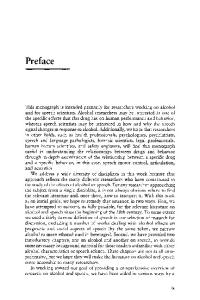
Figure 3.11 Cross-sections of spectra from the middle of English vowels of a male speaker, showing formants as spectral peaks.
variations in energy. Spectrograms portray only spectral amplitude, ignoring phase information, following the assumption that phase is relatively unimportant for many speech applications. While analog spectrograms have a dynamic range (from white to black) of only about )2 dB, the digitally produced spectrograms in this book have a greater range. Spectrograms are used primarily to examine formant center frequencies. If more detailed information is needed about the spectrum (e.g., resonance bandwidths, relative amplitudes of resonances, depths of spectral nulls), individual spectral cross-sections (displays of amplitude vs frequency) must be analyzed (Figure 3.11). Despite these limitations, spectrograms furnish much information relevant to acoustic phonetics: the durations of acoustic segments, whether speech is periodic, and the detailed motion of formants, As will be explained in Chapter 6, wideband spectrograms employ 300 Hz bandpass filters with response times of a few ms, which yield good time resolution (for accurate durational measurements) but smoothed spectra. Smoothing speech energy over 300 Hz produces good formant displays of dark bands, where the center frequency of each resonance is assumed to be in the middle of the band (provided that the skirts of a resonance are approximately symmetric).
3.4.2 Vowels Vowels (including diphthongs) are voiced (except when whispered), are the phonemes with the greatest intensity, and range in duration from 50 to 400 ms in normal speech. Like all sounds excited solely by a periodic glottal source, vowel energy is primarily concentrated below 1 kHz and falls off at about -6 dB/oct with frequency. Many relevant acoustic aspects of vowels can be seen in Figure 3.12, which shows brief portions of waveforms for five English vowels. The signals are quasi-periodic due to repeated excitations of the vocal tract by vocal fold closures. Thus, vowels have line spectra with frequency spacing of FOHz (i.e,
58
Chapter 3 •
Speech Production and Acoustic Phonetics
Iii Time
leI Time
10.1 (1)
'0
.E Q.. e -
:·
1 Time (5)
1.5
Figure 3.20 Spectrograms of English stops and nasals in vocalic context: /mi.unu.iti.utu.idi.udu/.
high F3. Discontinuities appear in formant slopes when the tongue tip makes or breaks contact with the alveolar ridge.
3.4.5 Nasals The waveforms of nasal consonants (called murmurs) resemble those of vowels (Figure 3.17b) but are significantly weaker because of sound attenuation in the nasal cavity. For its volume, the nasal cavity has a large surface area, which increases heat conduction and viscous losses so that formant bandwidths are generally wider than for other sonorants. Owing to the long pharyngeal + nasal tract (about 20 em, vs a 17 em pharyngeal + oral tract), formants occur about every 850 Hz instead of every 1 kHz. F 1 near 250 Hz dominates the spectrum, F2 is very weak, and F3 near 2200 Hz has the second-highest formant peak (Figure 3. 18c-e). A spectral zero, whose frequency is inversely proportional to the length of the oral cavity behind the constriction, occurs in the 750-1250 Hz region for [in], in the 1450-2200 Hz region for [u], and above 3 kHz for /111 [81]. Since humans have relatively poor perceptual resolution for spectral nulls, discrimination of place of articulation for nasals is also cued by formant transitions in adjacent sounds (Figures 3.1ge and 3.20). Spectral jumps in both formant amplitudes and frequencies coincide with the occlusion and opening of the oral tract for nasals. The velum often lowers during a vowel preceding a nasal consonant, which causes nasalization of the vowel (Figures 3.1ge and 3.20) (less often the nasalization continues into an ensuing vowel, if the oral tract opens before the velum closes). Vowel nasalization primarily affects spectra in the F 1 region: an additional nasal resonance appears near F I and the oral first formant weakens and shifts upward in frequency [82]; there is also less energy above 2 kHz [45].
Section 3.4
•
Acoustic Phonetics
65
3.4.6 Fricatives As obstruents, fricatives and stops have waveforms (Figure 3.17c-j) very different from sonorants: aperiodic, much less intense, and usually with most energy at high frequencies (Figure 3.18f-n). The reduced energy is due to a major vocal tract constriction, where airflow is (relatively inefficiently) converted into noise much weaker than glottal pulses. The obstruents of English and many other languages may be either voiced or unvoiced. Since acoustic properties can vary significantly depending on voicing, unvoiced and voiced fricatives are discussed separately. Unlike sonorants, in which the entire vocal tract is excited, unvoiced fricatives have a noise source that primarily excites the portion of the vocal tract anterior to the constriction, which results in a lack of energy at low frequencies. Unvoiced fricatives have a highpass spectrum, with a cutoff frequency approximately inversely proportional to the length of the front cavity. Thus the palatal fricatives are most intense, with energy above about 2.5 kHz; they have a large front cavity, since the constriction is a 10-12 mm wide groove behind the posterior border of the alveolar ridge [83]. With a groove 6-8 rom wide and further forward, the alveolar fricatives lack significant energy below about 3.2 kHz and are less intense. The labial and dental fricatives are very weak, with little energy below 8 kHz, due to a very small front cavity. The glottal fricative Ihl also has low intensity since the whisper noise source of the glottis is usually weaker than noise from oral tract constrictions, but energy appears at all formants since the full vocal tract is excited; in general, Ihl is a whispered version of the ensuing vowel. Voiced fricatives have a double acoustic source, periodic glottal pulses and the usual frication noise generated at the vocal tract constriction. The nonstrident voiced fricatives [v I and I blare almost periodic, with few noise components, and resemble weak versions of a glide such as IwI. The fricatives [z] and 13/, on the other hand, usually have significant noise energy at high frequencies typical of lsi and I f I, respectively. In addition, they exhibit a voice bar (very-low-frequency formant) near 150 Hz and sometimes have weak periodic energy in the low formants typical of sonorants. The spectra of unvoiced fricatives are rarely characterized in terms of formants because low frequencies are not excited and the excited upper resonances have broad bandwidths. Since the glottal pulses of voiced fricatives may excite all resonances of the vocal tract, however, formants can characterize voiced fricatives.
3.4.7 Stops (Plosives) Unlike other sounds, which can be described largely in terms of steady-state spectra, stops are transient phonemes and thus are acoustically complex (Figures 3.17i, j, 3.20 and 3.21). The closure portion of a stop renders the speech either silent (for most stops) or having a simple voice bar with energy confined to the first few harmonics (for some voiced stops). When present, the voice bar is due to radiation of periodic glottal pulses through the walls of the vocal tract; the throat and cheeks heavily attenuate all but the lowest frequencies. The release of the vocal tract occlusion creates a brief (a few ms) explosion of noise, which excites all frequencies, but primarily those of a fricative having the same place of articulation. After the initial burst, turbulent noise generation (frication) continues at the opening constriction for 10-40 ms, exciting high-frequency resonances, as the vocal tract moves toward a position for the ensuing sonorant. Unvoiced stops average longer frication than do voiced ones (35 vs 20 ms) [84]. In voiced stops, vocal fold vibration either continues throughout the entire stop or starts immediately after the burst. The vocal folds are more
66
Chapter 3 •
......... N :I: 4 ~ ........
apu
Speech Production and Acoustic Phonetics
uta
~
u
e 2
CJ
= c:r
4)
LI.
°0
0.5
1
1.5
Time (5)
...--.. N
%
4
~
~
>.
u c
2
CP
= tT
~
'- 00 u.
0.5
1
1.5
Time (5)
Figure 3.21 Spectrograms of the six English stops in vocalic context: / upc.ctn.nkn.cba.adc.agc.'.
widely separated during the closure for unvoiced stops and begin to adduct only near the time of release. Before the vocal folds begin to vibrate, a condition suitable for whisper usually occurs at the narrowing glottis. In such aspirated stops, the whisper source excites the resonances of the vocal tract, which are moving toward positions for the ensuing sonorant for about 30 ms after the frication period [84]. Unaspirated stops have little periodic energy at low frequency in the first 20 ms after stop release. Voiced stops in English are not aspirated, nor are stops after fricatives in initial consonant clusters. Other languages permit the independent specification of aspiration and voicing, thus creating four classes of stops. Stops are identified on spectrograms as sounds with very little intensity (at most a voice bar) for 20-120 ms during occlusion, often followed by a brief noise burst. Stops at the end of a syllable are often unreleased, in that little burst is apparent, due to a relaxation in lung pressure or a glottal stop, which reduces oral pressure behind the stop occlusion. Stops can be very brief between two vowels. Alveolar stops, in particular, may become flaps in which the tongue tip retains contact with the palate for only 10-40 ms. The shortest flaps occur between low vowels, where rapid ballistic motion is more feasible than between high vowels (due to the longer distance the tongue tip moves with low vowels) [58]. The burst release of alveolar stops is broadband, with energy primarily above 2 kHz. The peak for It/ is usually near 3.9 kHz, but it drops to 3.3 kHz before rounded or retroflex vowels; peaks for Idl are about 365 Hz lower than for [t], The different allophones of /kl lead to radically different burst spectra: a compact peak at about 2.7 kHz for /kl before a front vowel and a lower-frequency peak with a secondary peak above 3 kHz before a back vowel (the lower peak averages 1.8 kHz before unrounded vowels and 1.2 kHz before rounded vowels) [84]. Alveolar and velar bursts average about 16 dB weaker than ensuing vowels, while labial bursts are the weakest (28 dB less than vowels). The acoustics of affricates resemble that of stop + fricative sequences [61].
Section 3.4
•
Acoustic Phonetics
67
3.4.8 Variants of Normal Speech Common variants of normal speech are whisper, shout, and song. In whispered speech, the glottal periodic source for voiced speech is replaced by glottal frication (aspiration). Unvoiced obstruents are unaffected, but sonorants become unvoiced and decrease substantially in amplitude so that fricatives are louder than whispered vowels. At the other extreme of speech intensity is shouted voice, typically 18-28 dB louder than normal voice [85]. Both extremes suffer from decreased intelligibility, but for different reasons. In whisper, voiced and unvoiced obstruents are often confused. In shouting, the distinctions between many phonemes are sacrificed to increase amplitude so that the voice can be heard at a distance. Speakers often raise their voice intensity, without shouting, in inverse proportion to the distance from listeners (to compensate for the inverse square law of sound power radiating from the lips); FO level also goes up (but not FO range) and vowels lengthen [86,87]. Speakers also increase duration and intensity (among other factors) when faced with a noisy environment (the Lombard effect) [88,89]. Vowels, especially open vowels, dominate shouted speech in terms of duration. It is much easier to raise intensity for vowels than for obstruents, so shouting emphasizes vowels. Physiologically, the vocal tract tends to be more open for shouted than for normal voice, which raises FI and general amplitude but alters the speech spectra. The main difference, however, occurs at the glottis, where increased subglottal pressure raises amplitude, and altered vocal fold tension reduces the duration of the open phase in vocal fold vibration (similar glottal changes occur in emotional or stressed speech [90]). The resulting sharper glottal air puffs resemble square pulses rather than the normal rounded shape and thus have more high-frequency energy. FO also rises considerably, and formants tend to neutralize, deforming the vowel triangle [85]. Fundamentally, singing differs from normal voice mostly in intonation: (a) durations are modified to accomplish various rhythms, usually extending vowels (as in shouting) rather than consonants, and (b) FO is held fixed for musical intervals corresponding to different notes, rather than allowed to vary continuously as in speech. However, singing is often correlated with increased intensity (e.g., in opera), and singers can modify their articulations to have up to 12 dB more intensity via a fourfold increase in airflow with the same lung pressure [13.91]. One such change is a lowered larynx in vowels, which appears to add a singing forman! (also called vocal ring) at about 2.8 kHz, boosting energy by about 20 dB in the F3-F4 range, which is usually weak in normal voice [92]. This "formant" is actually a clustering of existing formants (F3-F5), and appears to relate to the narrow epilarynx tube (vocal tract right above the glottis). This tube is about 3 em long and 0.5 crrr' in area (vs 3 crrr' in the pharynx); being about ~ the length of the vocal tract, its quarter-wavelength resonance (see below) is about 3 kHz. Like the mouthpiece of a brass musical instrument, it matches a high glottal impedance to the lower impedance of the wider pharynx [93]. As we will see in Chapter 10, the style of speech significantly affects accuracy rates in automatic speech recognition. Spontaneous and conversational speech is the most difficult to recognize, due to its often faster rate, high use of words familiar to the listener, and frequent disfluencies. The latter include pauses at unexpected locations (e.g., within words), repetitions of portions of words, and filled pauses (e.g., "uhh" or "umm") [94]. At the other extreme, "hyperarticulate" or "clear" speech may be used when talking to computers or foreigners, on the assumption that such listeners cannot handle normal speech; such speech is slower with more pauses and fewer disfluencies [95].
68
Chapter 3 •
Speech Production and Acoustic Phonetics
Lastly, other human vocalizations include coughs and laughs. While not strictly speech, their analysis is relevant, especially in the context of speech recognition applications, where it would be useful to distinguish pertinent, linguistic sounds from other human sounds. Laughter usually consists of a series of 200-230 ms bursts of a breathy neutral vowel, often at higher FO than normal speech [96]. Coughs are irregular, brief: broadband noise bursts.
3.5 ACOUSTIC THEORY OF SPEECH PRODUCTION This section gives mathematical details for acoustic and electrical models of speech production that are suitable for many speech applications. Since more readers are familiar with electrical circuits than acoustics, electrical analogs of the vocal tract will be analyzed. Such analog models are further developed into digital circuits suitable for simulation by computer.
3.5.1 Acoustics of the Excitation Source In modeling speech, the effects of the excitation source and the vocal tract are often considered independently. While the source and tract interact acoustically, their interdependence causes only secondary effects. Thus this chapter generally assumes independence. (Some recent literature examines in more detail these interactions, e.g., influences on formants due to the subglottal regions, and on glottal flow due to supraglottal load, which is raised by oral constrictions [2]). In sonorant production, quasi-periodic pulses of air excite the vocal tract, which acts as a filter to shape the speech spectrum. Unvoiced sounds result from a noise source exciting the vocal tract forward of the source. In both cases, a speech signal s(t) can be modeled as the convolution of an excitation signal e(t) and an impulse response characterizing the vocal tract v(t). Since convolution of two signals corresponds to multiplication of their spectra, the output speech spectrum 8(0) is the product of the excitation spectrum £(0) and the frequency response V(O) of the vocal tract. This section models e(t) and £(0) for different types of excitation. Unvoiced excitation, either frication at a constriction or explosion at a stop release, is usually modeled as random noise with an approximately Gaussian amplitude distribution and a flat spectrum over most frequencies of interest. The flat range is about 2-3 octaves, centered on a frequency of U j(5A 3/ 2 ) (which equals typically 1kHz), where A is the area of constriction generating the noise and U is its volume velocity [17]. White noise, limited to the bandwidth of speech, is a reasonable model; in this case, 1£(0)1 has no effect on 18(0)1. The phase of £(0) is rarely analyzed because (a) spectral amplitude is much more important than phase for speech perception, and (b) simple models for random (unvoiced) e(t) suffice for good quality in speech synthesis. More research has been done on voiced than on unvoiced excitation because the naturalness of synthetic speech is crucially related to accurate modeling of voiced speech. It is difficult to obtain precise measurements of glottal pressure or volume velocity waveforms. Photography using mirrors at the back of the throat has shown how the glottal area behaves during voicing, but glottal airflow is not always proportional to glottal area because acoustic impedance varies during the voicing cycle (e.g., airflow follows the third power of glottal area
Section 3.5 •
69
Acoustic Theory of Speech Production
for small areas [62]). Two methods to measure glottal signals employ inverse filtering or a reflection/ess tube attached to the mouth. In inverse filtering, an estimate 1V(Q)I is made of 1V(Q)I, using the observed IS(Q)I and knowledge of articulatory acoustics. The excitation estimate then is simply
1£(0)1 = 1~(n)1 .
(3.1 )
IV(Q)I
A problem here is that errors are often made in estimating I V(Q)I, and this estimate is often adjusted to yield a smooth e(t), following preconceived notions of how glottal pulses should appear [97]. An alternative method extends the vocal tract with a long uniform tube attached to the mouth, which effectively flattens IV(Q)I by preventing acoustic reflections that would otherwise cause resonances. The spectrum of the output of the long tube should be I£(Q)I if the coupling at the mouth is tight and the entire system (vocal tract + tube) can be modeled as a long, uniform, hard-walled passageway. Since the vocal tract cross-sectional area is not uniform, however, certain distortions enter into I£(Q)I, especially for narrowly constricted vocal tract shapes [98]. The glottal volume velocity e(t) of voiced speech is periodic and roughly resembles a half-rectified sine wave (Figure 3.22). From a value of zero when the glottis is closed, e(t) gradually increases as the vocal folds separate. The closing phase is more rapid than the opening phase (thus the glottal pulse is skewed to the right) due to the Bernoulliforce, which adducts the vocal folds. A discontinuity in the slope of e(t) at closure causes the major excitation of the vocal tract; i.e., a sudden increase in Is(t)1 (Figure 3.12) every glottal period occurs about 0.5 ms after glottal closure (sound travels from glottis to lips in 0.5 ms). The duty cycle or open quotient (ratio of open phase-both opening and closing portions-to full period) varies from about 0.4 in low-FO shouts and pressed voice to above 0.7 in breathy, lowamplitude voices. To analyze voiced excitation spectrally, assume that one period of e(t) is a glottal pulse g(t). Periodic e(t) results in a line spectrum IE(Q)I because (a) e(t) can be modeled by the convolution of a uniform impulse train ;(t) with one pulse g(t), and (b) 1£(0)1 is thus the product of a uniform impulse train I/(Q)I in frequency and IG(Q)I. Since e(t) and thus ;(t) are periodic with period T = I/FO, both I/(Q)I and I£(Q)I are line spectra with FOHz spacing between lines. The relatively smooth function g(t) leads to a lowpass IG(Q)I, with a cutoff frequency near 500 Hz and a falloff of about - 12 dB / oct. Increased vocal effort for loud voices decreases the duty cycle of e(t), causing more abrupt glottal closure, hence a less smooth g(t) and more high-frequency energy in IG(Q)I.
o
A
A+B
T
T+A
2T
Figure 3.22 Simplfied glottal waveforms during a voiced sound.
Chapter 3 •
70
Speech Production and Acoustic Phonetics
3.5.2 Acoustics of the Vocal Tract Except for a falloff with frequency, the amplitudes of the spectral lines in IS(Q)I for voiced speech are determined primarily by the vocal tract transfer function I V(Q)I. A later section calculates IV(Q) I for a number of simplified models of the vocal tract. This section uses a general model to analyze vocal tract acoustics heuristically in terms of resonances and antiresonances. In its simplest model, speech production involves a zero-viscosity gas (air) passing through a 17 em long, hard-walled acoustic tube of uniform cross-sectional area A, closed at the glottal end and open at the lips. In practice, such modeling assumptions must be qualified: (a) vocal tract length varies among speakers (about 13 em for women, and 10 ern for 8-year-old children) and even within a speaker's speech (protruding the lips or lowering the larynx extends the vocal tract); (b) the walls of the vocal tract yield, introducing vibration losses; (c) air has some viscosity, causing friction and thermal losses; (d) area A varies substantially along the length of the vocal tract, even for relatively neutral phonemes; (e) while glottal area is small relative to typical A values, the glottal end of the vocal tract is truly closed only during glottal stops and during the closed phases of voicing; (f) for many sounds, lip rounding or closure narrows the acoustic tube at the lips. The effects of each of these qualifications will be examined in tum, but we ignore them for now.
3.5.2.1 Basic acoustics ofsound propagation. Sound waves are created by vibration, either of the vocal folds or other vocal tract articulators or of random motion of air particles. The waves are propagated through the air via a chain reaction of vibrating air particles from the sound source to the destination of a listener's ear. The production and propagation of sound follow the laws of physics, including conservation of mass, momentum, and energy. The laws of thermodynamics and fluid mechanics also apply to an air medium, which is compressible and has low viscosity. In free space, sound travels away from a source in a spherical wave whose radius increases with time. When sound meets a barrier, diffractions and reflections occur, changing the sound direction (variations in air temperature and wind speed also affect the direction of travel). At most speech frequencies of interest (e.g., below 4 kHz), however, sound waves in the vocal tract propagate in only one dimension, along the axis of the vocal tract. Such planar propagation occurs only for frequencies whose wavelengths A are large compared to the diameter of the vocal tract; e.g., for energy at 4 kHz,
A.
= elf = 340m/s = 8.5 ern, 4000/s
(3.2)
which exceeds an average 2 em vocal tract diameter. (The speed of sound e is given for air at sea level and room temperature; it increases at about 0.6 mls per °C [99], and is much higher in liquids and solids.) Due to its mathematical simplicity, planar propagation is assumed in this book, even though it is less valid at high frequencies and for parts of the vocal tract with large width. The initial discussion also assumes that the vocal tract is a hard-walled, lossless tube, temporarily ignoring losses due to viscosity, heat conduction, and vibrating walls.
Section 3.5 •
71
Acoustic Theory of Speech Production
Linear wave motion in the vocal tract follows the law of continuity and Newton's law (force equals mass times acceleration), respectively:
1 Bp
.
--+dlVV==O 2
p
(3.3)
at
pe
av
at + grad p == 0
(3.4)
where p is sound pressure, v is the vector velocity of an air particle in the vocal tract (a threedimensional vector describes 3D air space), and p is the density of air in the tube (about 1.2 mg/crrr') [98]. In the case of one-dimensional airflow in the vocal tract, it is more convenient to examine the velocity of a volume of air u than its particle velocity v:
u == Av,
(3.5)
where A is the cross-sectional area of the vocal tract. In general, A, U, v, and p are all functions of both time t and distance x from the glottis (x == 0) to the lips (x = /) (e.g., I = 17 ern), Using volume velocity u(x,t) and area A(x,t) to represent v under the planar assumption, Equations (3.3) and (3.4) reduce to au
I a(pA)
aA
- ax - -- pe -2- at + at '
(3.6)
Bp a(ujA) --==p--.
(3.7)
at
ax
For simple notation, the dependence on both x and t is implicit. While closed-form solutions to Equations (3.6) and (3.7) are possible only for very simple configurations, numerical solutions are possible by specifying A(x,t) and boundary conditions at the lips (for the speech output) and at the sound source (e.g., the glottis).
3.5.2.2 Acoustics of a uniform lossless tube. Analysis is simplified considerably by letting A be fixed in both time and space, which leads to a model of a steady vowel close to jaj. Other steady sounds require more complex A(x) functions, which are described later as concatenations of tube sections with uniform cross-sectional area. The analysis for a single long uniform tube applies to shorter tube sections as well. The tube is assumed straight, although actual vocal tracts gradually bend 90°, which shift resonant frequencies about 2-8 0/ 0 [100]. With A constant, Equations (3.6) and (3.7) reduce to au
A ap
ax == pe 2 at
and
_ ap
_!: au
ax -
A
at·
(3.8)
To obtain an understanding of the spectral behavior of a uniform tube, assume now that the glottal end of the tube is excited by a sinusoidal volume velocity source uG(t) and that pressure is zero at the lip end. Using complex exponentials to represent sinusoids, we have (3.9)
p(/, t)
=0
72
Chapter 3 •
Speech Production and Acoustic Phonetics
where 0 is the radian frequency of the source and V G is its amplitude. Since Equations (3.8) are linear, they have solutions of the form p(x, t) = P(x, O)e i nt (3.10) u(x, t) = U(x,O)e i n t, where P and U represent complex spectral amplitudes that vary with time and position in the tube. Substituting Equations (3.10) into equations (3.8) yields ordinary differential equations dU - dx = YP
dP - dx =ZU,
and
(3.11)
where Z = jOp1A and Y = jnA 1pc? are the distributed acoustic impedance and admittance, respectively, of the tube. Equations (3.11) have solutions of the form P(x, 0) = at eYx + a2e-Yx, (3.12) where the propagation constant y is
y=
m
(3.13)
=jQlc
in the lossless case (losses add real components to Z and ~ causing a complex y). Applying boundary conditions (Equations (3.9» to determine the coefficients a., we have the steadystate solutions for p and u in a tube excited by a glottal source: (x, t) P
=Z J
0
sin(Q(l- x)/c) U (Q)ei Q 1 cos(Qllc) G
= cos(n(/- x)/c) ( ) U x, t cos(nllc)
IT
VG
(n).Jnt ~~ e
(3.14)
,
where Zo = pcfA is called the characteristic impedance of the tube. Equations (3.14) note the sinusoidal relationship of pressure and volume velocity in an acoustic tube, where one is 90 0 out of phase with respect to the other. The volume velocity at the lips is ui], t)
= U(/. Q)e'
"nt
UG(Q)t!OJ = cos(QI/c) .
(3.15)
The vocal tract transfer function, relating lip and glottal volume velocity, is thus
vQ
_ U(/, Q) _ 1 ( ) - UG(Q) - cos(QI/c)
(3.16)
The denominator is zero at formant frequencies F; = n;/(21t), where Q;/Ic = (2i - 1)(1t/2) { F; = (2i - l)c/(4l)
fori= 1,2,3, ....
(3.17)
If I = 17 em, V(Q) becomes infinite at F; = 500, 1500, 2500, 3500, ... Hz, which indicates vocal tract resonances every 1 kHz starting at 500 Hz. For a vocal tract with a length l other than 17 em, these F; values must be scaled by 17/1. Linear scaling of formants for shorter vocal tracts of nonuniform area is only approximately valid because the pharynx tends to be disproportionately small as length decreases in smaller people [101,102]. Similar analysis using Laplace transforms instead of Fourier transforms shows that V(s) has an infinite number of poles equally spaced on the jn axis of the complex s plane, a pair of
Section 3.5 •
73
Acoustic Theory of Speech Production
~ F2
~ F3
Figure 3.23 Spatial distribution of volume velocity at frequencies of the first four resonances of an ideal vocal tract having uniform cross-sectional area. Places of maximum volume velocity are noted in a schematic of the vocal tract.
poles for each resonance at s, = ±j21tF;. Since a fixed acoustic tube is a linear time-invariant system, it is fully characterized by its frequency response V(O). The spectrum 8(0) of the tube output is thus VG(O)V(n), for arbitrary excitation V G as well as for the simple sinusoidal example of Equations (3.9). A tube closed at one end and open at the other resembles an organ pipe and is called a quarter-wavelength resonator. The frequencies at which the tube resonates are those where sound waves traveling up and down the tube reflect and coincide at the ends of the tube. As an alternative to the lengthy derivation above, vocal tract resonances can be heuristically computed using only boundary conditions and the phase relationship of pressure and volume velocity. Formant frequencies match boundary conditions on pressure P (relative to outside atmospheric pressure) and net volume velocity V: a closed end of the tube forces U = 0, whereas P ~ 0 at an open end. P is 90° out of phase with U, much as voltage and current are at quadrature in transmission lines or in inductors and capacitors. Given the boundary conditions and the 90° phase shift, resonance occurs at frequencies F;, i = 1, 2, 3, ... , where IVI is maximum at the open end of the vocal tract and IPI is maximum at the closed end. Such frequencies have wavelengths A; where vocal tract length I is an odd multiple of a quarter-wavelength (Figure 3.23): I = (A;/4)(2; - 1),
for i = 1,2,3, ... ,
(3.18)
which leads to Equation (3.17).
3.5.2.3 Resonances in nonuniform tubes. A uniform acoustic tube is a reasonable vocal tract model only for a schwa vowel. To determine formant frequencies for other sounds, more complex models must be employed. One approach that yields good models for many sounds follows perturbation theory. If the uniform tube is modified to have a constriction with
74
Chapter 3 •
Speech Production and Acoustic Phonetics
slightly reduced diameter over a short length of the tube, the resonances perturb from their original positions. The degree of formant change is correlated with the length and narrowness of the constriction. Consider a resonance F; with maxima in U and P at alternating locations along the tube. If the tube is constricted where U is maximum, F, falls; if P is maximum there, F, rises. In particular, a constriction in the front half of the vocal tract (i.e., between lips and velum) lowers FI, and a constriction at the lips lowers all formants, The effects on formants above Fl of constrictions not at the lips are complex due to the rapid spatial alternation of P and U maxima as frequency increases. This phenomenon derives from simple circuit theory. The relationships of volume velocity U (acoustical analog of electrical current l) and pressure P (analog of voltage V) can be described in tenns of impedances Z, involving resistance, inductance, and capacitance. As we will see later, modeling an acoustic tube by discrete elements (e.g., simple resistors, capacitors, and inductors) has severe drawbacks. A distributed model of impedances, as for a transmission line, is more appropriate for an acoustic tube. The mass of air in a tube has an inertance opposing acceleration, and the compressibility of its volume exhibits a compliance. The inertance and compliance are modeled electrically as inductance and capacitance, respectively. The local distributed (per unit length) inductance L for a section of tube with area A is p / A, while the corresponding capacitance C Following transmission line theory [1031 the characteristic impedance is is A /
pe-.
Zo = JL/C = pcfA,
(3.19)
If A is a function of distance x along the tube, then wide and narrow sections of the tube will have large values of C and L, respectively. In passive circuits such as the vocal tract, an increase in either inductance or capacitance lowers all resonant frequencies (e.g., the resonance ofa simple LC circuit is (2n~)-1), but in varying degrees depending on the distribution of potential and kinetic energy. Perturbing a uniform tube with a slight constriction reduces A at one point along the tube. If at that place, for a given resonance Fi, U is large without the constriction, kinetic energy dominates and the change in L has a greater effect on F; than do changes in C. Similarly, for those places where P is large, potential energy dominates and changes in C dominate F; movement. Since reducing A raises L and lowers C, F; increases if the constriction occurs where P is large and decreases where U is large [80]. Calculating the amount of formant change is left to a later section, but certain vocal tract configurations facilitate acoustic analysis. If the vocal tract can be modeled by two or three sections of tube (each with uniform area) and if the areas of adjacent sections are quite different, the individual tube sections are only loosely coupled acoustically, and resonances can be associated with individual cavities. Except for certain extreme vowels (e.g., /i,o.,u/), most vowels are not well represented by tube sections with abrupt boundaries; consonants, however, often use narrow vocal tract constrictions that cause A(x) to change abruptly with x at constriction boundaries. Thus, resonant frequencies for most consonants and some vowels can be quickly estimated by identifying resonances of individual cavities, which avoids the mathematical complexities of acoustic interaction between cavities.
3.5.2.4 Vowel modeling. The vowel /0,/ can be roughly modeled by a narrow tube (representing the pharynx) opening abruptly into a wide tube (oral cavity) (Figure 3.24a). Assuming for simplicity that each tube has a length of 8.5 cm, each would produce the same set of resonances at odd multiples of 1 kHz. Each tube is a quarter-wavelength resonator, since each back end is relatively closed and each front end is relatively open. At the boundary
Section 3.5 •
75
Acoustic Theory of Speech Production
lc 4--ll~
(c)
(b)
Figure 3.24 Two- and three-tube models for the vocal tract. In the two-tube case, the first tube section of area A I and length II may be viewed as modeling the pharyngeal cavity, while the second section of area A 2 and length 12 models the oral cavity. The first two models represent the vowels: (a) In/ and (b) [i], The three-tube model (c) has a narrow section corresponding to the constriction for a consonant. (After Stevens [104].)
between the tube sections, the narrow back tube opens up, whereas the wide front tube finds its area abruptly reduced. If the change in areas is sufficiently abrupt, the acoustic coupling between cavities is small and the interaction between cavity resonances is slight. Since each tube is half the length of the vocal tract, formants occur at twice the frequencies noted earlier for the single uniform tube. Due to actual acoustic coupling, formants do not approach each other by less than about 200 Hz; thus F 1 and F2 for / a/ are not both at 1000 Hz, but rather Fl = 900, F2 = 1100, F3 = 2900, and F4 = 3100. Deviations from actual observed values represent modeling inaccuracies (e.g., a simple two-tube model is only a rough approximation to I a/; nonetheless, this model gives reasonably accurate results and is easy to interpret physically. The respective model for Iii has a wide back tube constricting abruptly to a narrow front tube (Figure 3.24b). In this case, the back tube is modeled as closed at both ends (the narrow openings into the glottis and the front tube are small compared to the area of the back tube), and the front tube has open ends. These tubes are half-wavelength resonators because their boundary conditions are symmetrical: a tube closed at both ends requires U minima at its ends for resonance, whereas a tube open at both ends requires P minima at its ends. In both cases, the conditions are satisfied by tube lengths I that are multiples of half a resonance wavelength i.,.: 1_;
/ =-i 2
and
c
F; = ~ I",
ci
= 2/'
for i
= 1, 2, 3, ....
(3.20)
Thus, for Iii, both tubes have resonances at multiples of 2 kHz (again, in practice the formants of one tube are slightly below predicted values and those of the other are above,
76
Chapter 3 •
Speech Production and Acoustic Phonetics
when the tubes have identical predicted resonances). Besides the formants of Equation (3.20), another resonance at very low frequency occurs for vocal tract models containing a large tube (e.g., the back cavity) closed at both ends. This corresponds to Fl, which decreases from a value of 500 Hz in a one-tube model as a constriction is made in the forward half of the vocal tract. In the limiting case of a tube actually closed at both ends, F1 approaches a zerofrequency (infinite-wavelength) resonance, where the boundary conditions of minimal U at both ends are satisfied. In practice, F1 goes no lower than about 150 Hz, but many consonants and high vowels approach such Fl values. Back rounded vowels (e.g., /o,u/) can be modeled as having two closed tubes with a constricted tube between them; in such cases both F1 and F2 are relatively low.
3.5.2.5 Consonant modeling. A three-tube model appropriate for many consonants (Figure 3.24c) employs relatively wide back and front tubes, with a narrow central tube to model a vocal tract constriction. The back and central tubes are half-wavelength resonators (one closed at both ends, the other open at both ends), whereas the front tube is a quarterwavelength resonator. Thus, three sets of resonances F; can be defined: ci ci c(2i - 1) 21b ' 21e ' 41[
for i = 1, 2, 3, ... ,
(3.21 )
where Ib , Ie' ~ are the lengths of the back, central, and front tubes. Figure 3.25 shows how the front and back cavity resonances vary as a function of the position of the constriction, assuming a typical consonant constriction length Ie of 3 em, The resonances of the
,/'
F2~'"
----- ------
'F~
10
12
14
Length of back cavity (cm) Figure 3.25 Formant frequencies as a function of the length of the back tube in the model of Figure 3.24(c), using 16cm as the overall length of the three tubes and 3 cm as the constriction length. The dashed lines show the lowest two front cavity resonances, the solid lines the lowest four back cavity resonances. Dotted lines show the effect of a small amount of coupling between tubes, which prevents coinciding formant frequencies. The arrows at right note the formants (F2, F3, F4) of an unconstricted 16 cm long tube. (After Stevens [104] 1972 Human Communication: A. Unified View, E. David and P Denes (eds), reproduced with permission of McGraw-Hill Book Co.)
Section 3.5 •
Acoustic Theory of Speech Production
77
constriction occur at multiples of 5333 Hz and can be ignored in many applications that use speech of 4 or 5 kHz bandwidth. Labial consonants have virtually no front cavity, and thus all formants of interest are associated with the long back tube, yielding values lower than those for a single uniform open tube. A model for alveolar consonants might use a 10 em back tube and a 3 ern front tube; Figure 3.25 suggests that such consonants should have a back cavity resonance near 1.7 kHz for F2 and a front cavity resonance for F3 around 2.8 kHz. Alveolars are indeed characterized by relatively high F3 compared with average F3 values for vowels. Velar constrictions are more subject to coarticulation than labials or alveolars, but an 8.5 em back tube and a 4.5 ern front tube is a good model that leads to close values for F2 and F3 near 2 kHz. The dominant acoustic characteristic of velars is indeed a concentration of energy in the F2-F3 region around 2 kHz. If the velar has a relatively forward articulation (e.g., if it is adjacent to a forward vowel), F2 is a back cavity resonance and F3 is affiliated with the front cavity. The opposite occurs if the velar constricts farther back along the palate, e.g., when the velar is near a back vowel. A similar effect occurs between F3 and F4 for alveolar and palatal fricatives: lsi and I I might have 11 em and IOcm back tubes, respectively, which lead to a front cavity resonance of F3 for I I but of a higher formant for is]. The distinction between front and back tube resonance affiliation is important for obstruent consonants because speech energy is dominated by front cavity resonances. Frication noise generated just anterior to an obstruent constriction primarily excites the cavities in front of the constriction. Posterior cavities are usually acoustically decoupled from the noise source, until the constriction widens, at which point the noise ceases. Alveolars and front velars have dominant energy in F3, while F2 is prominent for back velars. Labial consonants with no front cavity to excite simply have low energy. In stop + vowel production, the stop release is marked by a noise burst that excites primarily the front cavities, giving rise to different spectral content for different stops. A velar constriction provides a long front cavity, with a low resonance near 2 kHz (F2 or F3). Alveolar resonances are higher (F4 and F5) due to shorter front cavities. The spectrum of a labial burst is relatively flat and weak since there is essentially no front cavity to excite.
J
J
3.5.2.6 Resonances and antiresonances. Postponing technical details, we can heuristically estimate the frequencies of antiresonances (zeros) in fricatives using simple acoustic tube models. When a sound source has only one acoustic path to the output (the mouth), the vocal tract frequency response has only resonances (poles) and no zeros. For nasals and obstruents, however, multiple acoustic paths cause zeros in the transfer function. In the case of fricatives, noise generated at a constriction outlet may propagate into the constriction as well as toward the mouth. At frequencies where the impedance looking into the constriction is infinite, no energy flows toward the mouth, and thus the output speech has antiresonances. A similar situation might be thought to occur at the glottis, i.e., sound energy could enter the lungs as well as the vocal tract. However, the glottal source is viewed as a volume velocity source, whereas frication noise is better modeled as a pressure source [62, but cf 105]. Zeros in voiced speech due to a glottal source are not considered part of the vocal tract response. Frication noise sources, on the other hand, have flat spectra with no apparent zeros. As a pressure source, the noise can be modeled in series with impedances due to the constriction and the front cavity. At those frequencies where the constriction impedance is infinite, no air flows and the output speech has no energy. This circuit analog holds for pole estimation as well. At the boundary between tubes of a two-tube model of the vocal tract, the impedance Zb looking back into the posterior tube is
78
Chapter 3 •
Speech Production and Acoustic Phonetics
in parallel with Zf looking forward into the front tube. In such a parallel network, resonances occur at frequencies where (3.22) For a tube closed or open at both ends, Z = 0 at frequencies where tube length is an even multiple of a quarter-wavelength; for a tube closed at one end and open at the other, Z = 0 where tube length is an odd multiple. If, on the other hand, tube length is an odd multiple in the first case or an even multiple in the second, then Z = 00. (Mathematical justification for these observations is given later.) When the boundary between tube sections is not abrupt enough to view the end of a section as fully open or closed, Z takes on intermediate values, and resonances cannot be associated with a single tube (as Equation (3.22) suggests). A simple two-tube model with abrupt section boundaries is valid for many fricatives, with a narrow back tube modeling the constriction and a wide front tube for the mouth cavity. The large pharyngeal cavity is ignored in such models because it is essentially decoupled acoustically from the frication excitation by the abrupt boundary between such a cavity and the constriction. The resonances of the pharyngeal cavity are canceled by its antiresonances in such cases. Thus, fricatives have resonances at frequencies where l.r is an odd multiple of a quarter-wavelength or Ie is a multiple of a half-wavelength. Conversely, zeros occur where Ie is an odd multiple of a quarter-wavelength. If alveolar fricatives /s,z/ are modeled with a 2.5 cm constriction and a 1 em front cavity, a zero appears at 3.4 kHz and poles at 6.8 and 8.6 kHz, with the two lowest frequencies being due to the constriction [106]. Palatal fricatives present a longer Ie and thus lower values for the first pole-zero pair, whereas dental and labial fricatives have very short Ie and i.r, leading to very high pole and zero locations. Fricatives have little energy below the frequency of their first zero and have energy peaks near the first pole frequency. Thus, in the frequency range of primary interest below 5 kHz, fricative energy is only at high frequencies, with more energy for the strident fricatives, having longer constrictions and longer front cavities.
3.5.3 Transmission Line Analog of the Vocal Tract Some insight can be gained into the spectral behavior of an acoustic tube by modeling it as a uniform lossless transmission line (T-line). Equations (3.8) (the acoustic wave equations)
R/2
~
L/2
(b) Figure 3.26 Two-port electrical network to model a length of uniform acoustic tube or transmission line: (a) "black box" showing input and output currents and voltages; (b) equivalent T-sectiontwo-port network; (c) realization of network with discrete components, which is valid if I is sufficiently small.
R/2 (e)
Section 3.5 •
79
Acoustic Theory of Speech Production
have a direct parallel with the behavior of voltage v(x,t) and current i(x,t) in a uniform lossless transmission line [103]: and
av
ai
ax
at'
(3.23)
--=L-
with the following analogies: current-volume velocity, voltage-pressure, line capacitance Cacoustic capacitance AIpc?, and line inductance L-acoustic inductance pIA. (As above, all inductances and capacitances are distributed, i.e., per unit length of tube or transmission line.) The acoustic impedance pc I A is analogous to Zo, the characteristic impedance of a transmission line. Using only basic properties ofT lines, we can easily calculate the frequency response of vocal tract models involving more than one acoustic tube in terms of T-line impedances. Consider a T-line section of length 1 as a two-port network, with voltages VI at the input and V2 at the output and current II into the T line and 12 out (Figure 3.26a). As a passive network, (3.24)
and
where ZII and Z22 are the input and output impedances of the T line, respectively, and Zl2 and Z21 are cross-impedances. By symmetry, ZI2
= -Z21
ZII
and
= -Z22
(3.25)
(the minus signs are due to the definition of /2 as flowing out of the T line and II into it). If /2 is set to zero by leaving the output port as an open circuit, ZII can be identified as the input impedance of an open-circuited T line [103]: ZII = Zo coth(yl),
(3.26)
where Zo and ~' are from Equations (3.19) and (3.13). If V2 is set to zero by making the output port a short circuit, Equations (3.24) give /2 /2 Z21 =-Z22-=ZII-' II II VI
(3.27)
= [Zo coth(yl)]I} + Z12 I 2 ·
In addition, VI can also be described via the input impedance ofa short-circuited T line [103]: (3.28) Thus Z21
(3.29)
= Zo csch(yl).
Under the assumption of zero pressure at the lips (Equation (3.9» and using Equation (3.13), we obtain the tube transfer function for current (or volume velocity): /2
J; =
V2 VI
Z21 = ZI.
=
Zo csch(yl) Zo coth(I'l)
1
1
= cosh(y/) =
cos(n/le)·
(3.30)
Thus, the same result for a lossless model of the vocal tract is obtained through T-line (Equation (3.30» or acoustic analysis (Equation (3.16». It is often convenient in circuit theory to model a symmetric network as a T section. The impedances of Figure 3.26(b) can be easily determined from Equations (3.25), (3.29) and (3.26) and simple circuit theory to be
Za = Zo tanh(~'/12)
and
Zb = Zo csch(y/).
(3.31)
80
Chapter 3 •
Speech Production and Acoustic Phonetics
If I is sufficiently small, the hyperbolic tangent and cosecant functions of Equation (3.31) can be approximated by the first terms in their power series expansions, e.g., tanh(x) = x -
x3
as
3" + 15 - ... ~ x,
if Ixl = lyl121
«
1.
(3.32)
Discrete components can thus replace the complex impedances in Equation (3.31):
1 yl Zb ~ Zo = I(G
and
+JOC).
(3.33)
The last steps of equation (3.33) simply assign values Rand G to the real parts of functions of y and 2o, and L and C to their imaginary parts, for the general case of a T line with loss. The earlier definition of y in Equation (3.13) assumed a lossless case, for which G and R would be zero. R represents viscous loss, which is proportional to the square of air velocity, while G represents thermal loss, proportional to the square of pressure; both Rand G also have components related to the mechanical losses of vibrating vocal tract walls [62]. The usual interpretation of R and L as resistors and inductors in series and of G and C as resistors and capacitors in parallel reduces Figure 3.26(b) to that of Figure 3.26(c) when I is small enough. The model using such discrete components in place of the usual distributed model is valid only if Iyll « 1. Assuming a frequency F in a loss less system,
Iy/l
= nile =
2nFlle« 1.
(3.34)
To model frequencies F below 4 kHz, I must be much less than 1.4 em. Thus an analog model of a 17 cm vocal tract using discrete components would require well over 20 T sections to accurately represent frequencies up to 4 kHz. A more practical analog representation would model each of the four resonances below 4 kHz separately, perhaps with an RLC network. The T-section model has the advantage of a close relationship to vocal tract shape (each impedance Za and Zb for a short section of the vocal tract model would be specified by its local crosssectional area), but building such a model is impractical. Indeed, all analog models are of little practical use because they are difficult to modify in real time, which is necessary to simulate time-varying speech. Models practical for speech simulation are discussed later.
3.5.3.1 Two-tube model: An earlier heuristic analysis for two-tube vocal tract models was limited to configurations with very abrupt tube-section boundaries and decoupled acoustic cavities. Equations (3.24}-(3.33) permit a resonance analysis of a general twotube model in which concatenated sections are modeled by T-line networks. A two-tube model can be viewed as a network in which two circuits are in parallel at the juncture between the two sections. At the juncture, the impedance 2 1 looking back into the first tube and Z2 looking up into the second tube serve to model the effects of the two circuits. The poles of a general circuit with N parallel components are those frequencies where their admittances add to zero: N
N
1
LYj=Lz.=O. ;=1 ;=1
(3.35)
I
A circuit of only two parallel components can also be viewed as a series circuit, where poles occur at frequencies for which impedances add to zero. With either approach, the poles of a two-tube model satisfy (3.36)
Section 3.5 •
81
Acoustic Theory of Speech Production
Since the glottal opening is usually much smaller than AI' the first tube (modeling the pharyngeal cavity) is assumed closed at the glottal end. In T-line analogs, an open circuit (zero current) models the closed end of an acoustic tube (zero volume velocity). Defining Zo; as the characteristic impedance of tube section i (Zo; = pcIA;), Equation (3.26) gives (3.37) where p = 01c in the loss less case. For unrounded phonemes, the mouth termination of the second tube is considered to be open, and the opening is modeled by a T-line short circuit. Thus, Equation (3.28) yields
22
= Z02 tanh(yI2 ) = j Z02 tan(p I 2 ) '
(3.38)
Combining Equations (3.36)-(3.38) gives
Al
cot({31 1) = -
A2
(3.39)
tan(pI 2 ) '
Models for several sounds (e.g., Ii, la/ ,3/) allow I) solution of Equation (3.39) in terms of formants F;: for i
= 12, which facilitates
= 1, 2, 3, ....
an explicit
(3.40)
More general cases have easy graphical solutions at those frequencies for which plots of the tangent and cotangent curves of Equation (3.39) intersect (Figure 3.27). There are intersections every I kHz on average (most easily seen in Figures 3.27c and d). For a model in which I} ~ 12 (e.g., Figure 3.27c), both curves have periods of about 2 kHz. For lal, A 2 » A I and pairs of resonances occur near odd multiples of 1 kHz; Iii conversely has pairs of resonances near even multiples of 1 kHz.
3.5.3.2 Three-tube model for nasals. The resonances for the three-tube model of Figure 3.24(c) are not as easily determined as for the two-tube case because two tube junctions must be considered. One approach, valid for a general model of N tube sections, determines the transfer function of NT-section circuits in series and then solves for the roots of its denominator [62]. For more insight, however, consider the three-tube model of Figure 3.28, which applies to nasal sounds. Since the nasal tube joins the rest of the vocal tract at the velum, the entire system can be modeled as three tubes (pharyngeal, nasal, and oral) joined at one point, with circuits for the three in parallel. The poles of such a model are specified by Equation (3.35) (using the notation of Figure 3.28): I
1
1
-+-+-=0,
z, z; z,
(3.41 )
where Zp = -jZop cot(Plp), Zm = -jZom cot(Plm), and Z; = jZon tan(pl n ) . The mouth and pharyngeal tubes have closed acoustic terminations, while the nasal tube is open. Its graphical solution is complex because of the interaction of three curves, but the dimensional similarity of the pharynx and nasal tubes allows a simplification. If Ip = In = 10.5 em, each of l/Zp and 1/ Z; has periods of about 1.6 kHz and the function 1/ Zp + 1/ Z; has infinite values about every 800 Hz. The mouth tube for nasal consonants is often significantly shorter than the other tubes (e.g., 3-7 em), A plot of the slowly varying -1 IZm vs the more rapid l/Zp + l/Zn
82
Chapter 3 •
Speech Production and Acoustic Phonetics
em2 A2 =1 cm2 1]=8 em 12 =1 em
A,=8
(a)
~
A, = ! em2 A 2 =7 cm2 /1 =1 em 12 =7 em (c)
4
~
j'l---.. . . . . . . .
ICII::__
FI-F3=750. I250,2700 HZ-4 ' - _......__._.....-...._ A,=6em 2A 2 =6cm 2
I lal
.............
.......L-_..-.IL.-_
__'
4
IJ=6em 12 =6cm
(d)
--+---~...=:iI
:
_~+------..~----II--- ~--+-
......_ - - I
.......
~
\
FI-F3= 500.1500,2500 Hz -4
o
3
1 2 Frequency (kHz)
Figure 3.27 Two-tube approximations to vowels /i,lE,o.,a/ and graphical solutions to their formant frequencies using Equation (3.39). The solid lines are the tangent curves, the dashed lines the cotangent curves; the vertical dashes note where the curves attain infinite values. (After Flanagan [62].)
~
=4,sq. em.
,
..
1~12.5
....
~-----_
em.
--UN
Ap =5 sq. em. \ \ \
, ~=6
I
I P =8.5 em.
I
sq. em.
.I1
~
IM=6.5'
rc-- - - - - - - - -".. - - -
cr· '-1
Figure 3.28 Three-tube vocal tract model for nasal consonants. Typical cross-sectional area and length values are noted for the pharyngeal, nasal and mouth (oral) cavities. The glottal source is modeled by a piston. Output volume velocity U" emerges from the nostrils. (After Flanagan [62].)
Section 3.5 •
Acoustic Theory of Speech Production
83
would note intersections roughly every 800 Hz, with additional intersections every period of
-l/Zm· Nasal consonants are characterized by (a) formants every 800 Hz (due to the longer pharynx + nasal tube than the normal pharynx + mouth tube), (b) wider formant bandwidths, and (c) zeros in the spectrum [107]. When airflow from the lungs reaches the velum junction, it divides according to the impedances looking into the mouth and nasal tubes. Spectral zeros occur at frequencies where Zm = 0, which results in no airflow into the nasal tube and thus no nasal speech output. Solving Zm = -j2om cot(21tF;lmlc) = 0 for F; yields zeros at odd multiples of c/4lm . The mouth tube for Im/ is about 7 ern, which gives zeros at 1.2, 3.6, 6.0, ... kHz. Shorter tubes for Inl and tn). about 5 and 3 ern, respectively, mean fewer zeros below 5 kHz: only one each at 1.7 and 2.8 kHz, respectively. Besides the poles due to the pharynx and nasal cavities, which occur every 800 Hz, nasal spectra have pole-zero pairs due to the mouth cavity; i.e., each zero is close in frequency to a mouth cavity pole. Nasalized vowels are much stronger than nasal consonants because virtually all airflow passes through the relatively unconstricted oral cavity, which reduces the role of the lossy nasal cavity. In terms of the three-tube model, the major difference between nasalized vowels and consonants is that the mouth cavity has an open termination, Thus Zm should be replaced by jZom tan(fJl m) in Equation (3.41). The major difference in pole positions between oral vowels and their nasalized counterparts is a shift in Fl and an additional nasal formant near F I [82]. Since much more sound exits the mouth than the nose in nasalized vowels, the nasal cavity is viewed as an acoustic side branch specifying zero frequencies (other small side branches off the vocal tract near the glottis, called piriform fossa, add spectral zeros near 4-5 kHz and slightly reduce lower formants [93,108]). The fixed nature of the nasal cavity suggests that zeros should not vary significantly for different nasalized vowels and should be found at frequencies F; where
Z; =jZon tan(21tFilnl c) = 0,
(3.42)
i.e., at odd multiples of about 1.7 kHz. The transition from an oral vowel to a nasal consonant (and vice versa) may involve an intermediate nasalized vowel sound, as the velum lowers before (or raises after) oral closure. As the velum lowers, nasal pole-zero pairs are created with the nasal tract as a side resonator. When the mouth cavity closes, these pairs disappear and other pole-zero pairs due to the mouth cavity appear. The process reverses for the release of a nasal consonant.
3.5.3.3 Three-tube model for fricatives. Unlike the previously modeled sonorants, virtually all obstruents have an excitation source in the oral cavity. From the noise source, sound waves at most frequencies flow out the mouth as speech, but some are trapped in cavities behind the source (via spectral zeros) and thus are not present in the speech output. This situation does not arise for sonorants, because the glottis closes at the primary excitation, forcing one-way airflow during the closed phase of voicing. While the poles of a transfer function for a system such as the vocal tract are independent of the location or type of excitation source, zeros are highly dependent on the source. In most unvoiced fricatives, the first few resonances (due to the back cavities) of the vocal tract have their spectral effects canceled by zeros. The three-tube model of Figure 3.24(c) is appropriate for many fricatives. The noise excitation is usually modeled as a pressure source at the juncture of the constriction and the front tube (Figure 3.29). For lsi, typical model parameters would be Ie = 2.5 cm, A c = 0.2 crrr'. and A h = At = 7 em", Due to the large AhlA e ratio, the back cavity is
84
Chapter 3 •
Constriction
Mouth cavity
10.2 cm 2
t:=~======::::.Source
--+--2.5
cm-----
Speech Production and Acoustic Phonetics
Noise sou rce Cavities behind source
7 cm 2
Cavities in front of source
(a)
(b)
Figure 3.29 Production models for fricatives: (a) a simplified model of the vocal tract for lsi; (b) an equivalent circuit representation. (After Heinz and Stevens [106] and Flanagan (62].)
effectively decoupled from the noise source and can be ignored. From Equations (3.19), (3.28), and (3.36), the poles of the remaining two-tube system occur where pc
Ze + Zf = j - tan(Qlelc) Ae
pc
+ jA-
tan(Q~/c) =
O.
(3.43)
f
Since Af » A e, poles occur near frequencies where Ze = 0 (half-wavelength resonances of the constriction) and where Zf is very large (quarter-wavelength resonance of the front tube). Zeros occur in the output speech spectrum where the impedance Z; of the constriction is infinite because no airflow circulates at those frequencies in a series network such as that of Figure 3.29(b). Z; = }ZOe tan(2nFile/c) becomes infinite at odd multiples of c/(4Ie) (i.e., when Ie is quarter-wavelength). For a 2.5 cm constriction, the first zero is at 3.4 kHz. As discussed earlier, palatal fricatives have longer values for Ie and If' resulting in lowerfrequency zeros and poles, whereas If,()1 have much higher zeros and poles. When the front tube is very short, its spectral effects can be ignored at most frequencies
of interest. A two-tube version of Figure 3.24(c) ignoring the front tube permits investigation of the effects of the large cavity behind the constriction, especially during transitions to and from the fricative, where the back cavity is not fully decoupled acoustically. Most lowfrequency poles are due to the back tube and occur near frequencies where cot(f31b) = 00 (half-wavelength resonances at multiples of 1360 Hz for Ib = 12.5 em), but poles also appear near fre.quencies where cot(fJle ) = 00 (half-wavelength resonances at multiples of6800 Hz for Ie = 2.5 em). The zeros can be shown [62] to solve (3.44) Since Ab » Ae and Ib » Ie' most zeros occur where tan(fJlb ) = 0 and effectively cancel out the corresponding poles of the back cavity. The uncanceled zeros occur where tan(f3le ) = 00, i.e., Ie is an odd multiple of quarter-wavelength (e.g., 3.4 kHz in the example). For some sounds (e.g., If/), the noise source is close to the junction between the back tube and the constriction [62]. Using the same two-tube model as above, the poles do not change, but the zeros can be shown to occur where (3.45)
Section 3.5 •
Acoustic Theory of Speech Production
85
i.e., where Ih is a multiple of half-wavelength. Again, the back cavity poles are canceled by zeros. 3.5.3.4 Four-tube vowel model: While a few vowels can be roughly approximated with only two tubes, others require at least three tubes due to a tongue constriction between the pharyngeal and oral cavities. Lip rounding can require a fourth short tube to model the lips (Figure 3.30). If the constriction length /2 is kept fixed at 5 ern (the middle six points), F2 falls and Fl rises as the back length /1 decreases. Note the similarity of Figures 3.30 and 3.25. In general, modeling accuracy improves as more (and shorter) tubes are employed, but complexity also increases with the number of tubes (Figure 3.31). Models of 2-4 tubes do not produce the spectra of natural sounds with great accuracy, but they have the advantage of insight into articulatory-acoustic relationships.
..X" (a) ...11
[1
(b)
4
N
3
~ >u
2
:t e cu
~
g-
cu
LA:
1
Length of back tube. II Constrictio coordinate•
x .I
r
0 15
14
12
10
8
6
17.5 16.5 14.5 12.5 10.5 8.5
4
2
0
0
6.5
4.5
2.5
.5
0
0
-1.5 -2.5
Length of front tube. I 3
0
0
0
0
2
4
6
8
10
12
14
15
Length of tongue, /2
0
1
3
5
5
5
5
5
5
3
1
0
Figure 3.30 Four-tube vocal tract model for vowels and their first three formants: (a) model in which the first three areas are fixed at A I = A 3 = 8 cm 2 and A 2 = 0.65 em 2 and the lip length /4 is fixed at I em; (b) curves 1, 2, 3, and 4 represent mouth areas of 4, 2, 0.65, and 0.16 cm 2 , respectively. The horizontal axis varies the lengths of the first three tubes. (After Fant [109] and Flanagan [62].)
86
Chapter 3 •
2 O~----.......,;;;;~-
~2
E
~
0....--------
... 2 QI 1a..J-----... 1 01--------~2
(a)
U
~
...
i.~---
01--------
;2
;;
A
.! 0 1 - - - - - - - - ~2 QI
:2 =
'- 0..-------:J
:a 0..-------~2
U Ot---------
2
u
00 5 10 15 20 Distance from glottis (em)
(b)
Speech Production and Acoustic Phonetics
II I I I I I I I I I I I I I II I I II II I o
I I1
2
I3
Formant frequency (kHz)
Figure 3.31 (a) The graphs show typical area functions for nine vowels, specifying the radius of consecutive! em long cylindrical sections of the vocal tract model; (b) corresponding measured formant frequencies. (After Stevens et al. [110].)
3.5.4 Effects of Losses in the Vocal Tract Under the assumptions of a hard-walled tube containing a zero-viscosity gas, there are no losses in the vocal tract. Resonances and antiresonances have zero bandwidth (i.e., poles and zeros on the jn-axis of the s plane or on the unit circle of the z plane), and electrical circuit models have no resistive components. In practice, however, losses are introduced at each step of the speech production process. When the glottis is open, a varying glottal impedance affects the spectrum of the glottal source. As air flows up the vocal tract, yielding walls react to pressure variations and vibrate, primarily at low frequencies due to the massive size of the walls. Viscous friction between the air and the walls, as well as heat conduction through the walls, causes energy loss. Big losses occur during nasals due to the large, yielding surface area of the nasal cavity. Finally, sound radiation at the lips adds significant energy loss. Viscous, thermal, and radiation losses occur primarily at high frequencies, since radiation losses are proportional to F 2 and the other two losses increase with P [62,111]. For the basic acoustic equations, terms would be added to Equation (3.6) to account for the volume velocity shunted by wall motion and to Equation (3.7) to account for viscous pressure drop [98]. Viewing losses in terms of formant bandwidths (which are proportional to the distance of the poles from the unit circle in the z plane), wall vibration is significant only below 2 kHz and dominates (along with glottal damping) the bandwidth of Fl. Radiation losses dominate formant bandwidths above 2 kHz. Friction and thermal losses can be neglected below 3-4 kHz, except for nasals.
Section 3.5 • Acoustic Theory of Speech Production
87
3.5.5 Radiation at the Lips Up to now, we have ignored lip radiation and assumed that sound pressure at the lips was zero (e.g., an electrical short circuit or an open termination for an acoustic tube). In practice, the lips are more accurately modeled as an opening in a spherical baffle representing the head [112], where a lip impedance ZL(n) describes the relationship of lip volume velocity UL(O) and pressure PL(Q): (3.46) ZL(n) can be modeled as a parallel RL (resistor-inductor) circuit, which acts as a highpass
filter with a cutoff frequency near 6 kHz. The L reactance models the effective mass of vibrating air at the lips. Thus ZL behaves like a differentiator: very small at low frequencies and growing at 6 dB / oct over frequencies of interest. A similar radiation effect occurs for nasal consonants, where sound radiates out the nostrils. The combination of vocal tract resonances (Equation (3.30» and losses (including radiation) produces the typical vocal tract transfer function of Figure 3.32. Actual speech spectra also include the effects of excitation.
3.5.6 Model of Glottal Excitation During the closed phase of voiced excitation, the vocal folds are shut, and the model of an electrical open circuit or a tube with a closed termination is accurate. Maximal glottal area during voicing is sufficiently small compared with the pharyngeal area to justify use of the same model even during the open phase for high frequencies. At low frequencies, however, a better model employs a glottal volume velocity source with a parallel glottal impedance ZG(Q), which is the ratio of the transglottal pressure head to the mass flow rate of air (24). ZG(Q) acts as a series RL circuit, whose impedance increases at 6 dB/oct above a certain break frequency. As with yielding vocal tract walls, ZG(Q) has its primary effects on the lowest formants, broadening their bandwidths. zG(n) is not a fixed impedance but oscillates with the vocal folds. This is most visible in the decay rate of a vowel waveform, which is dominated by the bandwidth of FI (and F2, if Fl and F2 are close). The main vocal tract excitation occurs at vocal fold closure, after which ZG(Q) is infinite and the FI bandwidth is
o -30
-60 4
1
5
Frequency (kHz) Figure 3.32 Frequency response for a uniform vocal tract relating lip pressure to glottal volume velocity.
88
Chapter 3 •
Speech Production and Acoustic Phonetics
small; when the vocal folds open, zG(n) decreases, widening F1, and the speech wave oscillations damp out more rapidly than when the vocal folds are closed [Ill]. Most speech models assume that the vocal tract and glottal source can be manipulated independently and have separate acoustic effects. For frequencies near F 1, however, the vocal tract impedance is comparable to the high glottal impedance, and significant source-tract interaction occurs [62]. Furthermore, sounds with a narrow vocal tract constriction produce a pressure drop at the constriction sufficient to affect the glottal source. The load of the vocal tract impedance skews glottal pulses away from a symmetric waveform and toward a more rapid closing phase [113]. Accurate modeling of vocal fold behavior may lead to improved quality in speech synthesis [114, 115]. For most sounds and frequencies, however, sourcetract independence is a good approximation that permits independent analyses of the glottal and supraglottal systems.
3.5.7 Quantal Theory of Speech Production The relationship between speech spectra and the vocal tract shapes that produce them is highly nonlinear. Large articulatory movements sometimes cause small acoustic effects, and other small movements yield large changes in formants. One theory of speech production [1 16] holds that sounds have evolved to take advantage of articulatory positions that can vary to a degree without causing large acoustic variations; e.g., spectra for the vowels /i,al correlate well with simple two-tube models, for which small changes in tube length have little effect on formant locations. Evidence for this quantal theory comes from both speech production and perception [68]. Changes in the manner of articulation often relate to the narrowness of a vocal tract constriction, while place of articulation relates to the position of the constriction along the vocal tract. Since changes in manner have larger acoustic effects than do changes in place, evidence that vertical tongue positioning is more accurate than horizontal location [117] supports the quanta I theory. The point vowels /i,a/, governed by one constriction, exhibit acoustic stability (i.e., steady formants) over a relatively wide range of constriction positions, while the acoustics is still highly sensitive to the degree of constriction, although motor commands show a quantaI (nonlinear) relationship with the degree [118]. The latter is not evident for lui, which exploits two constrictions (lips and pharynx) to control the formant patterns. Revisions of this theory of speech production (theory ofenhancement) hypothesize that: (1) distinctive features represent well the sounds of languages (with groups of such features simultaneously forming phoneme segments), (2) the acoustic manifestations ofa subset called primary features are more salient, and (3) features with varying degrees of strength can enhance each other [54].
3.6 PRACTICAL VOCAL TRACT MODELS FOR SPEECH ANALYSIS AND SYNTHESIS Analog speech production models employing electrical circuits or T lines are useful for understanding the behavior of airflow and pressure in the vocal tract and for predicting spectral resonances and antiresonances. For automatically generating speech, however, these models are too cumbersome, and digital models are invariably employed. One type of practical model is based directly on vocal tract shape, while another derives from the time and spectral behavior of the output speech signal and is only indirectly based on articulation. We examine the articulatory model first and the terminal-analog model later.
Section 3.6 •
Practical Vocal Tract Models for Speech Analysis and Synthesis
89
3.6.1 Articulatory Model A digital articulatory model of the vocal tract is an extension of earlier lossless multitube models, e.g., the two- and three-tube models that facilitated resonance analysis. For simplicity, the effects of vibration, friction, and thermal losses are included only in the glottal and lip termination models. Consider a model of N lossless cylinders of lengths I, and crosssectional areas Ai concatenated in series, where i runs from I at the glottal end to N at the lips (Figure 3.33). N is typically 8-12, which allows more accurate articulatory representation than is possible with only 2-3 tubes. For some sounds, however, even 1.4 cm sections (as with N == 12) are not short enough to yield accurate models. Earlier, we interpreted the basic laws of acoustics spectrally and established models relating vocal tract shape to the impedances of uniform tube sections or T lines. Whether heuristically relating tube or T line lengths to resonance wavelengths or explicitly solving for resonances in complex impedance relationships of vocal tract transfer functions, the spectral approach gave little insight into the time-domain behavior of sound waves. The most common digital model for the vocal tract, however, is based on time signal relationships.
3.6.1.1 Traveling waves. Returning to the basic acoustic laws for a time-domain interpretation, recall that Equations (3.8) hold for a loss less uniform acoustic tube and thus are followed in each of the N tube sections for the current model. To find the volume velocity ui(x, t) in the ith tube, combine Equations (3.8) into a second-degree equation:
cY-U
ax
2
I cYu == c 2 2 '
(3.47)
at
which has a solution of the form Ui(x, t)
== ui(t -
x/c) - uj(t
+ xf c),
(3.48)
where x is measured from the glottal end of each tube (0 ~ x ~ Ii). The pressure Pi(X, t) has a similar solution, which can be expressed in terms of Equation (3.48) as Pi(X, t)
pc
== -[ui(t - xlc) + uj(t + x/c)]. Ai
(3.49)
The functions ui(t - x/c) and uj(t + xl c) represent traveling waves of volume velocity moving up and down the ith tube (to the right and left in Figure 3.33), respectively.
Figure 3.33 Model of the vocal tract using a concatenation of four loss less cylindrical acoustic tubes, each of length l, and uniform cross-section area Ai.
--=:J C------I...-/4 ----. -11~134-/2-'
GLOTTIS
LIPS
90
Chapter 3 •
Speech Production and Acoustic Phonetics
Boundary conditions between sections are due to physical conservation principles, which specify continuity in both time and space for both p;(x, t) and u;(x, t). At the boundary between sections i and i + I, (3.50) where 't; = l;/c is the time for a sound wave to propagate through the ith section. The left side of Equation (3.50) is the net volume velocity u;(l;, t) at the left edge of the boundary, while the right side corresponds to u;+l (0, t) at the right edge. The parallel result for pressure is PAc [ui(t -
't;)
PC
+ uj(t + 't;)] = A
;
;+1
[U~l (t) + uH-l (t)].
(3.51)
In an analogy to T lines, when a traveling wave in a uniform tube meets a discontinuity in area, part of the wave propagates to the next section and part is reflected back. Propagation is 1000/0 only if the impedance of the next section matches that of the current section, i.e., if the sectional areas are the same or if the tube is terminated in a load impedance identical to the characteristic impedance of the present tube. This relationship is clarified by solving Equations (3.50) and (3.51) for the outgoing waves in tenns of the incident waves: Ut.I (t)
uj(t +
't;)
= {3;ui(t -
Ti) + riuH-1 (t)
= -r;ut(t - r;)
+ 80 dB) in sounds more complex than tones [38]. A small minority of fibers (about 9%) [39] have dynamic ranges greater than 60 dB, which could help explain the wide range of perceived sounds, but a more likely interpretation is that the timing patterns, as well as the average number, of firings affect perceived loudness [40-42]. 4.2.5.1 Timing of neural firings. The properties of a nerve fiber are often measured using histograms of spikes, in response to many click and tone stimuli over long durations. These displays show the number of firings at specific time delays with respect to each other or to the sound stimulus: post-stimulus histograms record the delay relative to the initiation of the stimulus, period histograms show the delay relative to the (sometimes arbitrarily defined) "start" of each period in a periodic stimulus, and interval histograms display the times between successive firings (Figure 4.7). These histograms have shown that firings tend to be synchronized with displacements of the basilar membrane in a certain direction. When the 8M vibrates sinusoidally with sufficient amplitude, a nerve fiber tends to fire on synchronous half-cycles of the movement at the point where the fiber is attached. Histograms of the times of the spikes (synchronized to the period of the sound stimulus) closely resemble half-wave rectified versions of the 8M movement near the neuron (Figure 4.8). There also appears to be a form of automatic gain control (with an approximate response time of 20 ms), by which loud and soft stimuli yield very similar timing histograms; i.e., higher probability of neural firing at peaks in the sound waveform, relatively independent of its amplitude. In response to input clicks, preferred firing times are well modeled by a delay plus a multiple of the inverse of the fiber's CF. The delay (up to 3 ms at the BM apex) is well
118
Chapter 4 •
(c)
(b
12
(a)
408 Hz
e .5 o ~
850 Hz
72/5
~ 60
1000 Hz 182/5
179/5
....
~
5
'o
(e
(d) .!12 ~
z
60
o Figure 4.7
~
III
II II
2000 Hz
234/5
10
10
15
20
(f)
1500 Hz
E
Hearing
2300 Hz
178/5
15 20 5 1 Duration of interval (ms)
83/s
o
5
1
Interval histograms of a fiber with a 1.6 kHz CF. The average response rate in spikes/s is indicated for six different 1 s tone burst excitations (at 80 dB). (After Rose et a/. [43].)
20
70 dB
,c:!
~ tlOO
2'0
1 ms Figure 4.8
Time
~
Period histograms of a fiber activated by a low-frequency tone. Each plot is fitted with a sinusoid corresponding to the stimulus frequency, with varying amplitude but fixed phase. The bin width or horizontal (time) resolution in this figure is coarse compared with that of Figure 4.7. (After Rose et a/. [43].)
modeled by the propagation time for a traveling wave from the stapes to the hair cell in question. Several firings in response to one click are possible, depending on the click's intensity. With tone stimuli, the spikes tend to occur at intervals of multiples of the period of the input tone. In each case, there is some time jitter (usually less than 1 ms) in the actual firing times; i.e., the intervals between firings are not perfect multiples of the BM period. Each neuron normally fires just prior to maximal membrane displacement. Neurons have a latency period of 1-3 ms in which, having once fired, a neuron cannot fire again, no matter how intense the stimulus. Thus at low frequencies of BM motion (e.g.,
Section 4.3 •
Sound Perception
119
below 1 kHz), a neuron could fire on each half-cycle of a sinusoidal vibration, and the spikes would be time-synchronized (phase-locked) to a tonal sound input. At higher frequencies, the latency period is too long to allow such synchronous firings, although a set of adjacent neurons would exhibit an average synchronous pattern. Above about 4-5 kHz, phase locking disappears due to the smearing in time caused by jitter, which becomes comparable in range to the fundamental period. With an input of two sinusoids, phase locking in a fiber may occur with one or both tones, depending on their relative intensities and how close their frequencies are to the fiber's CF [5l
4.2.6 Adaptation An auditory neuron can fire at rates up to 1000/s for short periods of time in response to a sudden loud stimulus, but if the sound remains, the neuron adapts slowly and decreases its firing rate by about half (exponentially with a time constant r of about 40 ms, relatively independent of signal level). Most of the decay occurs in the first 15-20 ms after stimulus onset (especially at high stimulus intensities) [44, 45]. When the stimulus is removed, the firing rate falls to near zero and then exponentially increases back to the spontaneous rate characteristic of the neuron (the recovery time constant is about 2.S!, and is larger for neurons with lower spontaneous rates [46]). This behavior can be explained in terms of depletion and regeneration of the chemical transmitter substance in the hair cells associated with the neuron. Adaptation is more pronounced and has a more complex form for neurons higher in the auditory nervous system than for those in the cochlea. Such adaptation suggests that the brain may interpret sound intensities and some spectral information from changes in firing patterns rather than from steady-state patterns. There may be two classes of auditory neurons: one that responds primarily to steady-state sounds and another that fires more often when the stimulus is of rapidly changing frequency. This sensitivity of the latter class to change in frequency persists over a wider range of sound intensities than is the case for the steady-state neurons. Indeed, the sensitivity is more pronounced near normal sound levels such as in speech (physiological levels) than at levels near the hearing threshold. This contrasts with steadystate neurons, which often have saturated firing rates at physiological levels. Neurons in the cochlear nucleus and at higher levels exhibit recoding of the cochlear firings, in that they often respond in a complex fashion with respect to the sound stimulus, e.g., responding only to the start or end of a stimulus [5].
4.3 SOUND PERCEPTION The primary questions in sound perception [5, 47] concern what sounds are perceptible, what a person hears, and how different sound components affect or interfere with one another. Whether a sound can be heard depends on its intensity and spectrum; we discuss perceptibility in terms of hearing thresholds. What a person hears in response to a sound is a more complicated question, and we will initially limit our discussion to how a sound's structure relates to its perceived pitch. Finally, we address the complex question of masking or interference. The behavior of the ear in response to simple tones is relatively straightforward, but most sounds are dynamic and have many spectral components. The cochlear processes of basilar membrane vibration and neural firings are highly nonlinear, with the result that perception of sound energy at one frequency is dependent on the distribution of sound energy at other frequencies as well as on the time course of energy before and after the sound.
120
Chapter 4 •
Hearing
4.3.1 Auditory Psychophysics Auditory psychophysics is concerned with the resolving power of audition. Basic sounds such as tones and clicks are often used as acoustic stimuli. How well listeners can discriminate the timing and frequencies of such sounds is likely relevant to speech perception. However, experiments using stimuli closer to speech (than clicks and tones) lead to a more direct correspondence between the acoustic aspects of a speech signal and how it is perceived. Asked to discriminate two similar sounds resembling speech, listeners may utilize linguistic knowledge, attempting to label the stimuli as different linguistically (e.g., as representing different phonemes). Alternatively, they may simply listen for some salient difference in timing or spectral content. Listeners are much better at discriminating two sounds than at labeling them; e.g., they can distinguish tones near 100 Hz to within 1 Hz accuracy, but cannot consistently group such tones into fine categories such as 100, 101, 102, ... Hz. A typical listener, in ordering a set often tones at 1 Hz intervals from 100 to 109 Hz, must listen to them in pairs, each time deciding which is higher.
4.3.2 Thresholds The ear is capable of hearing sounds over a wide frequency range, from about 16 Hz to 18 kHz. (This range of about 10 octaves is much larger than that for vision-about 0.7 oct, from infrared to ultraviolet.) Sounds of frequency below 1 kHz or above 5 kHz require significantly more energy to be heard than those in the 1-5 kHz range (Figure 4.9). The intensity of a sound is measured in terms of sound pressure level (SPL) in units of decibels (dB). The reference level for SPL is an intensity of 10- 16 W/cm2 (0.0002 dyn/crrr' or ubar of pressure) at a frequency of 1 kHz, which corresponds to 0 dB. At the extreme frequencies of the audible range, sounds can be perceived only over a narrow amplitude range, whereas at the frequencies where the ear is most sensitive (1-5 kHz), sounds are detectable over a range of more than 100 dB (which slightly exceeds the 90 dB range for vision). The minimum intensity at which sounds can be perceived is called the auditory or hearing threshold, which rises sharply with decreasing frequency below 1kHz and with increasing frequency above 5 kHz. This spectral bandpass effect is due both to the filtering action of the outer and middle ear and also to the smaller number of hair cells toward extreme CFs. Loud sounds can actually be felt in the ear, which leads to two other thresholds: of feeling (the intensity at which a sound is felt) and of pain (intensity causing pain). These upper thresholds are much less variable with frequency than the auditory threshold is; e.g., the pain threshold is near 120-140 dB for all frequencies in the auditory range, whereas the auditory threshold varies over a 100 dB range. Speech normally occupies only a portion of the range between the thresholds of hearing and pain (known as the auditory field). With frequencies ranging from 100Hz up to perhaps 8 kHz, speech has amplitudes between 30 and 90 dB (measured at a distance of 1 m from the lips). Since speech has dynamic intensity, we can define a slowly varying speech level that reflects the peak SPL over periods of the order of a second. Speech perception is optimal when peak amplitudes are in the 60-70 dB range. The auditory threshold remains almost constant across most speech frequencies; e.g., between 700 and 7000 Hz the hearing threshold stays within ±3 dB of 0 dB. While the threshold increases substantially above 7 kHz, speech energy at such high frequencies is significantly present only for fricatives and has little effect on either speech intelligibility or naturalness. The threshold is more relevant for frequencies below 700 Hz, which is the region of the first formant as well as the fundamental frequency and its most intense harmonics. At
Section 4.3 •
121
Sound Perception
Feeling
12
--r-r--------I ., "T" T T -, - r - -
10
I
.........
I 1
I
•
•
.,
-,-,- r ., - r -
CO
"C
T I
"'-'
>,
~
9V; C OJ
,iJj
..:
60
40
Hearing
20 O+----+---+----IIo-----+--.;~..:.-~..:.-...;..-~'--_+_-.....
20
50
100
200
2 00 5000
10000
Frequency (Hz) Figure 4.9
The areas of speech perception inside the limits of overall hearing. The partition grid corresponds to the auditory differential limen (Section 4.4) of pitch and loudness under the influence of wideband noise. The lowest curve is also known as an audiogram and can vary by up to 20 dB in individual listeners of normal hearing. (After Winckel 1968 Acoustical foundations of phonetics, B. Malmberg (ed) in Manual of Phonetics, Amsterdam: NorthHolland [48].)
an average F1 of 500 Hz, the hearing threshold is elevated by about 10 dB compared to the F2-F3 regions. A typical FO at 100 Hz needs almost 40 dB more intensity to be heard than harmonics at higher frequencies. For vowel sounds at physiological levels (those typical of speech), all the harmonics are normally audible (but not equally loud) up through F4, with harmonics between formants at higher frequencies sometimes falling below audibility. However, as speech amplitude is reduced, e.g., in quiet speech, it is likely that the fundamental and its first few harmonics are lost perceptually. These frequencies are not crucial to intelligibility since, for example, speech is understood over the telephone network, which severely attenuates frequencies below 300 Hz. While irrelevant for intelligibility, frequencies below 300 Hz contribute to naturalness, and their lack is one aspect of the quality limitations of telephone speech. The hearing threshold concerns the detectability of steady tones. If the sound duration is less than 0.3 s, the threshold is elevated since overall energy becomes important for perceiving short stimuli. For wideband noise, sounds under 0.3 s, the threshold increases about 3 dB for
122
Chapter 4 •
Hearing
each halving of duration [47]. In tones with changing frequency (tone glides) and very short duration (50 ms), the hearing threshold can be higher by up to 5 dB for falling than for rising tones [49, 50]. This can be relevant for transition sounds in speech, where most spectral movement at phoneme boundaries occurs over durations of less than 50 ms. It is difficult to extrapolate the audibility of speech sounds from these tone thresholds because hearing is a nonlinear process; the detectability of a sound consisting of many spectral components is not a simple function of the detectability of its components.
4.3.3 Just-Noticeable Differences (JNDs) Most psychophysical experiments use sounds that differ along one or more acoustic dimensions (e.g., intensity or FO) but are otherwise identical. Listeners are asked whether two successive sounds are identical (AX procedure: does X sound the same as A?), or are presented with three sounds and asked which of two of the sounds resembles most the third (ABX or AXB procedure: does X sound closest to A or B?). The first technique is most common and yields a plot of percentage "different" responses as a function of the acoustic difference. If the acoustic dimension varied is perceptually relevant, the plot typically goes from a low percentage ("same") to a high percentage ("different") monotonically as the acoustic difference increases. The acoustic value at which 75% of responses are "different" is normally selected as the just-noticeable difference (JND) or difference limen. In the second procedure (ABX or AXB), X is the same as either A or B, and the number of correct identifications increases as the difference between A and B increases; the point where subjects correctly identify 75% of the stimuli is the JND. An alternative procedure, which tends to yield smaller JND values, asks listeners to adjust some parameter of a sound to resemble a reference sound; the standard deviation of selected parameter values provides the JND [51]. JNDs are relevant for both speech perception and coding: JNDs measure the resolving power of the ear and the limits of audition, and suggest how precisely speech parameters need to be quantized for transmission. Due to the frequency variation in auditory thresholds, the perceptual loudness of a sound is specified via its relative intensity above the threshold. A sound's loudness is often defined in terms of how intense a reference I kHz tone must be, to be heard as equally loud as the sound. Loudness units are called phons and are identical to dB for tones near 1 kHz. At speech frequencies, equal-loudness contours parallel the hearing threshold curve (Figure 4.9). At low frequencies, however, 1 dB can have the effect of two phons (Figure 4.10). The JND for loudness is essentially constant at about 0.5-1.0 dB for noise bursts, but varies for tones: ranging from 0.3 dB in optimal conditions (e.g., a 60 dB tone at 1 kHz) to more than 1 dB at low intensities; they also increase with frequency at low levels [52]. Greater JNDs are found at very high intensities [53] or with durations less than 250 ms [47]. Sounds of equal intensity increase in loudness with duration up to about 200 ms. Another measure of loudness is the sone, by which a doubling of loudness is equivalent to an intensity increase of about IOdB. Below 1 kHz, two equally intense tones must differ by about 1-3 Hz to be distinguished in frequency. At higher frequencies, the JND is progressively larger (e.g., at 8 kHz, it is 100 Hz) [47, 55]. The JND increases substantially if the sound is weak or brief, i.e., less than 20 dB above threshold or shorter than 100 ms. Over the entire auditory field, there are about 1600 distinguishable frequencies and 350 such intensities, leading to about 300,000 tones of different combinations of frequency and intensity that can be distinguished by listeners in pairwise tests [48, 56]. People in general cannot, however, identify so many tones in isolation;
Section
~.3
•
Sound Perception
123
14
(ij
>
---~ 100
10
Phons 80
~ QJ ~
~ 60
CJ ~
Q.
-c
40
40
c
5
20
20
~'---
C/)
o
Minimum audible field
-,/ - - - - - - - - - - __ ;' /
-21 ......-~....--+---....---+--+-----+------+-~ .02 .05 0.1 0.2 0.5 1.0 5.0 20.0 Frequency (kHz) Figure 4.10
Equal-loudness contours as a function of tone frequency. (After Robinson and Dadson [54].)
they must be heard in successive pairs. (Those few who possess "absolute pitch," and thus have the musical ability to name tones without context, do not appear to have smaller JNDs [57J.) The figures above are valid for sounds lasting more than 100-200 ms; the ear is less sensitive with shorter sounds. For example, there are 850 distinguishable frequency levels for tones of more than 250 ms, but only 120 levels for 10 ms tones. Similarly, the number of discriminable intensities is halved as duration decreases to 10 ms. Other sounds are less precisely perceived than tones; e.g., for narrowband noise bursts, only 132 frequency steps and 120 intensities can be distinguished, which represents only 5% of the number of distinguishable tones.
4.3.4 Pitch Perception Distinguishing two tones (or other periodic sounds) is usually done through pitch, the perception of the "basic" frequency of a sound. Pitch is usually affiliated with periodic sounds, and most closely corresponds to the fundamental rate of sound vibration; it is however much more complicated than a simple acoustic: perceptual mapping of FO: pitch. A sound is said to have a certain pitch if it can be reliably matched to a tone by adjusting the tonal frequency (usually using a 40 dB sine) [58]. Sounds lacking periodicity can be said to differ in timbre [59], e.g., /s/ has brighter timbre than / J/ because /s/ has most energy at higher frequencies; timbre reflects a sound's spectral envelope. Information relevant to a sound's perception can be obtained from the rates and timing of neural firings at different locations along the basilar membrane. A sound's loudness may be perceived in proportion to the overall rate of neural firings, but spectral perception is more complex. The timing or volley theory holds that low frequencies, e.g., those corresponding to the first harmonics of the fundamental frequency (FO) in speech, are perceived in terms of time-synchronous neural firings from the 8M apex. The place theory, on the other hand,
124
Chapter 4 •
Hearing
suggests that, especially for higher frequencies such as those in the formants of speech, spectral information is decoded via the 8M locations of the neurons that fire most [6]. Thus there are two types of pitch: the "normal" pitch corresponding to the inverse of the fundamental period of the sound (FO), and a "spectral" (or place) pitch corresponding to timbre (e.g., /ul with its low-frequency concentration of energy sounds lower in spectral pitch than does Iii). The normal pitch is also called residue or virtual pitch since it is perceived even when the FO component is absent [60]. For example, in speech over the telephone, the fundamental and harmonics below 300 Hz are absent, yet a pitch corresponding to an FO of 100 Hz would be detected by the presence of higher harmonics separated by 100 Hz each. Virtual pitch can be regarded as the perceived repetition frequency of a periodic sound and is apparently determined by the positions of about the eight lowest harmonics [61, 62]. The harmonics in the Fl region are especially important for pitch perception. Even though pitch is most naturally associated with temporal repetition, pitch perception seems to follow spectral measures (e.g., harmonics) more closely than changes in the time signal; in particular, changes in the phases of harmonics do not affect pitch but change waveform structure [63]. When speech is simulated with one sinusoid per formant ("sinusoidal speech," with three tones centered at three formant frequencies), unnatural speech results, but pitch usually follows the tone at the F1 frequency [64]. Phase is less important than other perceptual factors, but listeners can distinguish a phase shift of 2-4° in one harmonic of a complex tone when phases are set to zero (but not when randomized) [65]. Some sound stimuli give conflicting pitch cues. For example, short clicks of alternating polarity every 5 ms have an FO of 100 Hz but a pulse rate of 200 pulses/so The BM displacement resolves each pulse in time at its basal, high-frequency end, and associated neurons fire in cycles of200/s [8]. However, the apical end vibrates sinusoidally near 100 Hz, leading to time-synchronous neural firings there at FO. When there are sufficient timesynchronous firings at the base (usually the case for FO above 100 Hz), they dominate the perception of pitch. At lower rates, even the apical end of the 8M resolves the pulses in time, and the perceived pitch corresponds to the pulse rate, not FO. The same results occur with complex waveforms whose phase is inverted every half-period, which suggests that neural time patterns are insensitive to phase inversions in low-frequency stimuli [66]. Such ambiguous pitch seems to arise mostly when a stimulus has a small number of high-frequency harmonics within a critical band (see below), leading to unresolved harmonics (i.e., ones interacting within a single auditory filter) [60, 67]. Indeed, the FO JND increases with the frequency of the lowest harmonic in such sounds. The place theory is supported by the varying frequency sensitivity with displacement along the BM and by the tonotopic organization of neurons in the auditory pathway to the brain. The maximal vibration of a specific BM location in response to a tone could be signaled to the brain by a pathway "labeled" cognitively with the tone frequency. The timing theory instead presumes that the central nervous system can convert timing patterns into pitch. This theory is limited to low and middle physiological frequencies because the synchronization of spikes to tonal inputs disappears above 4-5 kHz (due to latency effects), whereas the place theory cannot explain the high pitch resolution of the ear to low frequencies. It is likely that both processes operate in parallel, with one or the other dominant depending on the frequency and type of sound [68]. One theory holds that spectral selectivity in the cochlea serves to separate broadband sounds into a number of channels, within which temporal analyses are performed [69]. Another recent model uses inhibitory gating neurons [70].
Section 4.3 •
Sound Perception
125
4.3.5 Masking An important aspect of hearing is the phenomenon of masking, by which the perception of one sound is obscured by the presence of another. Specifically, the presence of one sound raises the hearing threshold for another sound, for sounds heard either simultaneously or with a short intervening delay. Simultaneous sounds cause frequency masking, where a lowerfrequency sound generally masks a higher-frequency one (such masking can be directly related to speech recognition in low-frequency noise [71]). Sounds delayed with respect to one another can cause temporal masking of one or both sounds. Masking is the major nonlinear phenomenon that prevents treating the perception of speech sounds as a summation of responses to their tone and bandlimited noise components. In some speech coding applications, quantization noise that arises in the coding process can be distributed across frequencies to take advantage of masking effects, such that the noise may be masked by high speech energy in the fonnant regions. Masking involving tones (e.g., harmonics in speech) and noise is thus especially relevant. Classic masking experiments show the effect of one tone on another as a function of the frequency separation between them [61, 72]. With a stimulus consisting of two tones above the threshold of hearing, a listener tends to hear only the lower-frequency tone in certain conditions. If one tone is fixed at 1200 Hz and 80 dB, a second tone below 800 Hz can be heard as low as 12 dB. However, when that second tone is within 100 Hz of 1200 Hz, it needs at least 50 dB to be heard. This masking effect remains for higher frequencies as well: at least 40 dB is required for the second tone (up to 4 kHz) to be perceptible. In general, low frequencies tend to mask higher frequencies, with the largest effects near harmonics of the low-frequency masker. Masking effects are usually described with functions of a masked threshold (the energy a masked signal needs to be heard) or the amount ofmasking (the additional energy needed to hear the signal in the presence of the masker) as a function of signal frequency (Figure 4.11 ). Such psychophysical tuning curves are obtained using simple perceptual experiments and provide analogs to the tuning curves of auditory fibers [73]. The actual inhibition of neural firings caused by a masker can be displayed via suppression areas superimposed on tuning curves (usually just outside the curve's skirts), which indicate the amplitude required, as a function of frequency, for a tone to act as a suppressor. The mechanism for such suppression may be saturation [74]. When tones are used as both signal and masker, the analysis is complicated by beats and combination tones, which can change masked thresholds by more than 10 dB near the frequencies of the difference tones; e.g., in response to tones at fi and h Hz (ji e
U
ell
= CT
~
2 : : : : :.:: :: : : . ••••••
.:.. ~.~. • • ••••••• . ..••• p •••••
K
.. ..®
. W rM :::
..... "::.:::::'" ::::::::::::::::::"/# ~.~:::
1
~.~.~.~
...
~
~
·.:·2t:.:.~~!~:~S:~~S~f·. : : : :. •1
.................... • • • • M •••••• .................... ~
o
•
••••• •••••• •••••
e
•
• • • • • • • • • • • • • • • • • • • e •••••••••••••••••
a
o
u
Figure S.S Listeners' identification as /p,t,k/ in response to synthetic CV stimuli of a noise burst followed by a steady two-formant vowel. The vertical axis indicates burst frequency, while different vowels are displayed horizontally. In each column, the two bars note the positions of Fl and F2. The size of the symbol (circles for [t], slanted lines for /k/, dots for Ip/) indicates the relative number of listener responses. (After Cooper et al. [8].)
transition dominates place perception; i.e., if the VC and CV transitions provide conflicting place cues, listeners perceive place according to the CV transition [89]. Finally, although the primary cues to place are spectral, VOT and amplitude also playa role. When F2 and F3 transitions give ambiguous cues in synthetic CV stimuli, VOT duration can distinguish labial from alveolar stops [90]. Changes in spectrum amplitude at high frequencies (F4 and higher formants) can reliably separate labial and alveolar stops: when high-frequency amplitude is lower at stop release than in the ensuing vowel, labials are perceived [91]. In general, more intense release bursts lead to perception of alveolars rather than labials [92].
5.5.2.2 Static onset vs dynamic spectral transitions. Certain aspects of spectral patterns of releases in voiced stops appear to distinguish place of articulation. The concentration or spread of energy (diffuse vs compact) and whether the main spectra) trend is rising, flat, or falling with frequency have been suggested as crucial spectral cues [22, 23, 93]. Manipulating burst spectra and initial formant frequencies in synthetic CV stimuli led to unambiguous place identification when the onset spectrum was either diffuse-falling (/b/), diffuse-rising (/d/), or compact (/g/) (see Figure 3.38). Stimuli with spectra not fitting any of the three categories yielded equivocal responses from listeners. When the stimuli were
Section 5.5 •
157
Consonant Perception
truncated to 10-46 ms versions of the original CV syllables (starting at stop release), place identification was good, even when the noise burst was eliminated and when the second and higher formants held steady. Thus the gross properties of the spectrum during the initial 10-20 ms of a stop consonant provide important cues to place perception. When the initial spectrum is ambiguous (e.g., diffuse but flat), listeners apparently utilize formant transitions to distinguish place. Such transitions temporally link the primary place cues in the stop release to the slowly varying vowel spectrum, with no abrupt spectral discontinuities after the stop release. In this view, the formant patterns act as secondary cues, which are invoked when the primary cues of the release spectrum are ambiguous. The performance of this model was evaluated by comparing listeners' judgments of place in isolated CV syllables with the model's predictions based on the initial CV spectra. The model achieved 85% accuracy for CV syllables, but only 760/0 for yes; furthermore, nasal consonants performed more poorly. One problem with this model is that the proposed templates involve fixed loci, which is at variance with earlier experiments [7]. The templates emphasize static acoustic features rather than dynamic ones, and much other evidence points to the relevance of spectral changes [94]. Dynamic aspects of the CVover the initial 40 ms are likely crucial for stop perception [95]. For example, velar stops are poorly identified (730/0) on a basis of only the first 20 ms of natural CV stimuli, and when stimuli contain cues conflicting between onset spectra and formant transitions, listeners apparently rely more on the dynamic cues [96]. The relevant cues may not reside in the formant transitions per se, but in other timedependent spectral features, e.g., VOT, spectral tilt, presence of mid-frequency spectral peaks, abruptness of energy onset at high frequencies, and onset of a prominent low-frequency peak [97]. Labial and alveolar/ dental stops can be distinguished by a metric involving relative change in energy at high and low frequencies between burst and voice onset: the labials show equal or less change at low frequencies than at high frequencies [98]. Formant transitions, however, seem to be the most important cues for stop place perception [99], e.g., locus equations (straight-line regression fits to critical points in formant transitions) [100].
5.5.2.3 Interaction of cues. Perception of place of articulation and other consonant features are interdependent. In synthetic voiced stops and nasals, place can be reliably cued by F2-F3 transitions, but the boundaries on formant continua between labials and alveolars are not the same for stops as for nasals [101]. The same holds for voiced stops and weak voiced fricatives [102]. Such interactions between place and manner perception appear to occur at the phonetic (and not auditory) level since place boundary shifts can occur with identical acoustic stimuli perceived differently as to manner (due to ambiguous manner cues) [103]. One possibility to explain the shift in the case of stops and fricatives is that slightly different places of articulation are involved: Ibl is a bilabial with an extreme forward place of articulation and I dl has a constriction farther to the rear than either IfI or I (}I, which have intermediate constriction points. Thus the perceptual boundary along an acoustic continuum of F2 and F3 'is likely to be different for stops and fricatives. Coarticulation appears to affect perception in various ways. Normally the distinction between lsi and / f I follows the steady-state frication energy: energy at lower-frequency cues If/. (Since these fricatives differ only in the place feature, discriminating between the two is done by place perception.) Formant transitions to and from the fricative provide secondary cues, due to the coarticulation of the fricative with adjacent phonemes. When a fricative with spectrum ambiguous between lsi and I f I is followed by a rounded vowel or an unrounded vowel, listeners tend to hear lsi or I I, respectively [104]. The effect occurs with synthetic
J
158
Chapter 5 •
Speech Perception
stimuli and also when naturally spoken phonemes are concatenated with synthetic ones. Similar perceptual shifts along stop continua occur when a stop ambiguous between ItI and Ikl is preceded by either Is/ or I JI [105] and when a stop ambiguous between Idl and Igl is preceded by III or [t I [106]. These effects exhibit a form ofperceptual compensation for the presumed coarticulation that occurs in natural speech production. For example, in the context of a rounded vowel, natural fricative spectra are shifted lower, and listeners expect to hear lower-frequency energy in a fricative adjacent to a rounded vowel; thus they shift their perceptual boundary so as to hear lsi with more low-frequency energy than occurs next to an unrounded vowel. The fricative-vowel effect shrinks in proportion to the temporal separation between frication offset and ensuing vowel onset and also varies with the presumed sex of the synthetic voice, both of which imply that listeners use tacit knowledge of speech production during speech perception. These phenomena could be due to auditory contrast or nonsimultaneous masking, but a phonetic interpretation is more likely, in which the listener integrates disparate acoustic cues (frication noise and formant transitions) in phoneme identification.
5.5.3 Perception of Voicing in Obstruents The linguistic feature voiced is used to distinguish the voiced class of obstruents
Ib,d,g,v,o,z,31 from the unvoiced class Ip,t,k,f,o,s,fl. For obstruents, voiced does not simply mean "having vocal cord vibration." Phonemic perception of the voiced/unvoiced distinction in stops and fricatives is correlated with a diverse set of acoustic properties. Fricatives provide the simpler case, with voicing usually perceived when the speech signal is periodic during the steady portion of the fricative. If vocal cord vibration produces enough energy at the fundamental and low harmonics (the voice bar on spectrograms), voiced fricatives are heard, at least for syllable-initial fricatives. Voicing perception in syllable-final fricatives (which have weaker periodicity) involves multiple cues; e.g., the duration of frication affects its voicing perception: shorter fricatives tend to be heard as voiced, and vice versa [107]. 5.5.3.1 Syllable-final obstruents. One voicing cue for both stops and fricatives in syllable-final position is the duration of the preceding vowel. Given that many syllable-final "voiced" obstruents have little vocal cord vibration, the primary cues may be durational: voicing is perceived more often when the prior vowel is long and has a higher durational proportion of formant steady state to final formant transition [108]. The ratio of vowel duration to consonant duration in ves has also been proposed to distinguish final consonant voicing since final voiced obstruents tend to be shorter than unvoiced counterparts; however, the data favor consonant and vowel durations as independent voicing cues [109]. It is not the physical duration of a preceding vowel that determines consonant voicing, but rather its perceived length; e.g., equal-duration vowels are perceived to be longer when FO varies rather than remains monotonic [110]. Thus, with VC durations ambiguous as to consonant voicing, voiced identifications increase with FO variation during a synthesized vowel [111]. Because FO patterns do not vary consistently before voiced and unvoiced stops, caution must be used in generalizing this last result (and others) to natural speech. English stop voicing perception is complex, in part because most voiced stops consist primarily of silence during the closure interval, with the voice bar much less in evidence than in other languages. Therefore, the obvious cue of vocal cord vibration is less available to distinguish stop voicing. However, even in other languages where voiced stops are truly "voiced" (vocal cord vibration throughout the oral closure), the situation remains far from
Section 5.5 •
Consonant Perception
159
simple. In French vowel-l-stop sequences, the duration of the closure, the duration and intensity of voicing, and the intensity of the release burst, as well as the preceding vowel duration, all affect voicing perception [1 12]. While most English voiced stops show little periodic structure, in VC contexts the glottal vibration in the vowel usually continues into the initial part of a voiced stop, whereas voicing terminates abruptly with oral tract closure in unvoiced stops. This difference in voice offset timing appears to be a primary cue to voicing perception in final English stops [I 13]. When a naturally produced syllable ending in a voiced stop has enough "voicing" removed (by substituting silence for periods of the speech signal) around the VC boundary, the corresponding unvoiced stop is heard. Since removing glottal periods from the vowel effectively lowers the durational V: C ratio, such an effect cannot be due to the primary cue of duration noted above. Rather, acoustic analyses of the stimuli reveal that unvoiced stops tend to be heard with high F I offset frequencies and short amplitude-decay times, suggesting rate of voicing offset as the crucial cue.
5.5.3.2 Syllable-initial stops. Voicing in syllable-initial stops involves interactions between temporal factors (VaT and the timing of the Fl transition) and spectral aspects (intensity and shape of the FI transition). It has been argued [114] that the diverse acoustic cues available for voicing perception in stops are all due to laryngeal timing with respect to the oral tract closure and that the listener integrates the varied acoustic cues into one voicing decision, based on the implicit knowledge that they arise from a common articulatory source .. The primary cue seems to be VaT: a rapid voicing onset after stop release leads to voiced stop perception, while a long VaT cues an unvoiced stop. Along a continuum of VOT, the voicedunvoiced boundary is near 30 ms, with shifts of about 5-10 ms lower or higher for labial or velar stops, respectively [101]. Thus perception appears to compensate for production: in natural speech, VOT decreases with the advancement of place of articulation, and in perception longer VOTs are needed to hear an unvoiced stop as the constriction moves farther back. A secondary cue to initial stop voicing is the value of F I at voicing onset [115]: lower values cue voiced stops. This again follows speech production since F 1 rises in CV transitions as the oral cavity opens from stop constriction to vowel articulation. Thus, F 1 rises during the aspiration period and is higher at voicing onset after longer VOTs. The duration and extent of the F 1 transition significantly affect stop voicing perception [116], whereas the behavior of the higher formants has little effect. Natural stop--vowel sequences do not always have a clear boundary between the end of aspiration and the onset of voicing (e.g., voicing often starts in F 1 while higher formants still have aperiodic structure). Confining periodic energy to the fundamental for the first 30 ms of voicing has little effect on perceived stop voicing, but more voiced stops are heard if voicing starts simultaneously in all formants (rather than just in F 1) [117]. A third cue to stop voicing is aspiration intensity. The perceptual salience of vaT may not reside in duration but in integration of aspiration energy. Listeners may utilize VOT differences as voicing cues, not in terms of timing judgments but rather via detection of presence vs absence of aperiodic aspiration [33]. Many psychoacoustic experiments note the salience of energy integrated over time; e.g., equally loud stimuli can trade duration for amplitude, with integrated energy being the perceptually relevant parameter. Thus, listeners may judge a stop to be unvoiced if they hear enough aspiration after stop release rather than using direct temporal cues.
160
Chapter 5 •
Speech Perception
Finally, when the primary acoustic cues to voicing are ambiguous, spectra and FO can affect voicing perception in CV sequences [90]. Recall that, when an obstruent is released into a vowel, FO starts relatively high if the consonant is unvoiced, and low if voiced. When VOT is ambiguous as to voicing in synthetic stimuli, rising FO at stop release cues stop voicing, and falling FO signals an unvoiced stop [118]. However, the FO cue is easily overridden by VOT in normal circumstances. The secondary voicing cues trade with VOT; e.g., changes in FI onset values can shift the voiced-unvoiced boundary along a VOT continuum. Before open vowels, a 1 Hz change in F 1 onset is perceptually equivalent to a 0.11 ms change in VOT [119]. Similarly, a VOT decrease of 0.43 ms is equivalent to a 1dB increase in aspiration intensity [120]. This sensory integration of spectral and temporal cues to make phonetic decisions does not appear to be restricted to speech sounds [121].
5.6 DURATION AS A PHONEMIC CUE Hearing utterances of syllables in isolation, listeners can distinguish phonemes with very short stimuli. If normal isolated vowels are cut back so that only the first few periods are presented, listeners can identify (above chance levels) tongue advancement and height features based on the first 10 ms alone, but they need 30 ms to distinguish the tense-lax feature [122]. The stop place of articulation in CVs can be identified based on the first 10 ms after release, but the voicing feature requires about 22 ms (voicing in velar stops requires the longest duration, 29 ms). It appears that longer portions of the stimuli are needed to discriminate certain phonemes, namely those whose distinguishing features involve timing as well as spectra: duration is crucial for the tense-lax vowel distinction and voicing in stops (VOT), but tongue advancement (place of articulation) and height can be specified by the spectra of the first 10 ms. Trading relationships may exist in durational perception at other levels [123].
5.6.1 Manner Cues Unlike some languages (e.g., Swedish and Japanese), English does not use duration directly as a phonemic cue, in the sense that phonemes differ only by duration and not spectrally. Nonetheless, with synthetic speech, duration alone can cause phonemic distinctions, which suggests that duration can be a secondary phonemic cue utilized when a primary cue is ambiguous; e.g., in the word rabid, the fbi closure duration is normally short; if the closure is artificially prolonged, rapid is heard. The tendency for unvoiced sounds to be longer than voiced sounds apparently affects perception. Since the stop follows the stressed vowel here, VOT is a reduced voicing cue, being short in both voiced and unvoiced cases. Thus, the cues for voicing may be found in the durational balance between the stop and the preceding vowel [124]. Similarly, when enough silence is added after lsi in slit, it sounds like split. In normal /spf clusters, the /p/ release is weak; thus the lack of a burst (in the extended version of s_lit) is insufficient to deter the perception of a stop. Normally a short, silent interval (about 10 ms) intervenes between the cessation of frication in a fricative+sonorant cluster and the onset of voicing. When this duration exceeds about 70 ms, the listener apparently decides that the interval is too long for a transition between phonemes and must itself be a stop phoneme. Silence duration interacts in a trading relation with spectral cues in signaling the presence of a
Section 5.6 •
Duration as a Phonemic Cue
161
stop here. The amount of duration necessary to hear a stop is greater if the formant transitions are more appropriate for slit than for split (conflicting cues) [125]. Stop duration also trades with (a) burst amplitude and duration in say-stay continua (e.g., stay is heard with a very short stop closure if the stop release burst is strong enough) [126] and (b) glottal pulsing in the perception of voicing in stops [127].
5.6.2 Place Cues An apparent secondary cue for place perception in stop consonants in stressed ev contexts is the duration of VOT. Due to coarticulation, labial stops have the shortest VOTs, while velar stops have the longest, with bigger differences (of about 40 ms) occurring in unvoiced stops. Labial stops permit tongue movement in anticipation of the ensuing vowel, which allows more rapid voicing onset since the vocal tract attains a proper vowel configuration more rapidly than for alveolars or velars. The velars have the longest VOTs, presumably because the tongue body moves slowly (compared to the tongue tip, used in alveolars) and because the tongue body usually must move for an ensuing vowel. Place perception in stops is affected not only by the duration ofVOT but also by closure duration in some cases. Stop closures tend to be longer for labials than for alveolars or velars, and the listener's tacit knowledge of this production fact appears to affect perception: longer stops are biased toward labial perception [92]. As another example, if a silence interval of 100-200 ms occurs between two synthetic vowels and formant transitions are ambiguous as to place, listeners tend to hear two separate stops (i.e., VeeV) [128]. If the initial ve transition specifies one stop, an ambiguous CV transition is perceived as a different stop, presumably because the listener expects two different stop consonants with a silence interval of sufficient duration between two vowels. If the silence interval is short (~25 ms), the CV transition dominates in place perception of one stop [129]. If the silence is greater than 200 ms, a pause instead tends to be perceived.
5.6.3 Speaking Rate Effects In virtually all situations where duration can function as a phonemic cue, its effect is relative to speaking rate [10, 130]. Segment durations both before and after a given phoneme affect that phoneme's recognition when duration is a critical identification cue [131]. For example, with an acoustic continuum Ibal- Iwal where the duration of the initial formant transitions cues the manner of articulation, longer transitions are needed to hear Iwal as the syllable is lengthened [132]. As syllable duration is increased from 80 to 300 ms, the Ibl - IwI boundary increases from transitions of 28 ms to 44 ms. Listeners apparently judge the abruptness of the transition in relation to speaking rate or syllable duration, assuming slower average transitions with slower speaking rates. The effect is nonlinear, most likely because duration is not the only cue to phonemic identity and because rate changes do not affect all speech events equally. The effect also appears to be local; i.e., the durations of adjacent phonemes have much more perceptual effect than phonemes more distant [133]. Finally, the effect tends to shrink under conditions closely approximating natural speech [134]. Coarticulation and formant undershoot are dependent on timing, with the percentage of time that vowels have steady-state formants decreasing as speaking rate increases. Listeners apparently compensate for coarticulation in interpreting different formant patterns in eve contexts (with different consonants) as the same vowel. They also seem to compensate for speaking rate since identical syllables preceded by syllables spoken at different rates cause
162
Chapter 5 •
Speech Perception
varying vowel perception [135, 136]. In hearing a syllable excised from a sentence, listeners assume the syllable was spoken in isolation with relatively long duration and little presumed formant undershoot, and thus they tend to misidentify the vowel. If the syllable is placed in a context where the speaking rate is different from the original utterance, listeners interpret the inserted syllable accordingly, judging the vowel duration and amount of formant undershoot in proportion to what would normally occur at the new speaking rate. Since duration is a secondary cue to vowel perception (i.e., some vowels with ambiguous formant cues are heard as tense if long and lax if short [136]), it is not clear whether listeners normalize vowel perception based on anticipated duration or formant undershoot. Similar speaking rate effects occur in consonant perception. If the closure duration of /p/ in topic is lengthened, listeners hear top pick, but the boundary threshold is a function of the contextual speaking rate. At faster rates, a given rendition is more likely heard as top pick [137]. Similar results occur for slit-split [133]. The VOT boundary for voicing perception in stop-l-vowel syllables can be shifted by up to 20 ms through manipulations of speaking rate [138]; similar effects occur with the duration of the burst release [139]. Voicing perception is most affected by the durations of the immediately adjacent context of the stop and can be cued equally through the steady-state durations of neighboring vowels or the durations of consonant transitions [138]. Furthermore, the effect of preceding context decreases as a function of the duration of any silence gap that occurs just prior to the stop. Finally, the phonemic effect of speaking rate is primarily due to the articulation rate (syllables per second) rather than the proportion of time spent in pauses, even though both factors contribute to the overall perception of speaking rate [132]. Compensations for speaking rate are not always straightforward. The distinction between fricative and affricate (e.g., shop, chop) is cued by the duration of frication, the duration of any preceding silence, and onset characteristics of the noise [32]. A normal trading relationship is found between the duration of silence and frication: long frication tends to cue a fricative, while long silence cues an affricate [140]. When contextual speaking rate is varied, however, more silence is needed to hear the affricate at faster rates. One possible explanation is that, as speaking rate changes, frication duration normally changes more than silence duration, and the listener perceptually compensates for the overall effect of rate and also uses inherent knowledge of which acoustic segments vary more or less with rate changes. Silence duration may be perceived differently when cueing a manner distinction rather than a voicing distinction.
5.7 INTONATION: PERCEPTION OF PROSODY Thus far this chapter has concentrated on how listeners perceive and discriminate individual sounds. Another important aspect of speech perception concerns prosody, whose domain of variation extends beyond the phoneme into units of syllables, words, phrases, and sentences. The perception of rhythm, intonation, and stress patterns helps the listener understand the speech message by pointing out important words and by cueing logical breaks in the flow of an utterance. The basic functions of prosody are to segment and to highlight. Cues in rhythm and intonation patterns notify the listener of major syntactic boundaries, which help one to mentally process speech units smaller than the entire sentence. The alternation of stressed and unstressed syllables identifies the words that the speaker considers important to understand the speech message and also helps in word comprehension (via placement of lexical stress). Besides segmenting utterances, prosody signals other aspects of syntactic structure. In many languages, a question requesting a yes/no answer from a listener ends with an
Section 5.7 •
Intonation: Perception of Prosody
163
intonation rise. There are usually cues in the choice of words or word order that also signal that the utterance is a question (e.g., subject-verb inversion: "Has Joe studied?"). However, sometimes the only cue lies in the intonation (e.g., "Joe has studied?"). Intonation can also signal whether (a) a clause is main or subordinate, (b) a word functions as a vocative or an appositive, (c) the utterance (or a list of words) is finished. While prosody usually helps a listener segment utterances perceptually, it can also serve as a continuity guide in noisy environments. This prosodic continuity function is very useful when there are several competing voices and the listener attempts to follow a specific voice. Experiments with two equal-amplitude voices have shown that listeners use intonation continuity and separation of pitch to follow one voice [141]. Even if two voices are presented binaurally through earphones and periodically switched between ears, listeners find it easiest to concentrate on one voice if its FO range differs from the other voice and if the FO contour is reasonably smooth (especially at the times when the voices switch between ears). Aspects of phase also seem to playa role in identifying simultaneous vowels [59]. Prosody also provides cues to the state of the speaker; attitudes and emotions are primarily signaled through intonation. FO and amplitude patterns vary with emotions [142], emotions often raise FO and amplitude levels and their variability [143, 144], increased FO range sounds more "benevolent" [145], and emotions (e.g., anger, sorrow, and fear) cause changes in FO., timing, articulation precision, average speech spectrum, and waveform regularity of successive pitch periods [146, 147]. Prosody is so important to normal speech perception that communication can occur even with severely distorted segmentals [148]: if speech is spectrally rotated so that highfrequency energy appears at low frequency and vice versa, segmental information is effectively destroyed. Nonetheless, subjects can converse under such conditions by exploiting the preserved aspects of FO, duration, and amplitude.
5.7.1 Stress: Lexical and Sentential There are two levels of stress in speech: lexical (word) stress, and sentential (phrase) stress. At the word level, one syllable in each word is inherently marked to receive stress, but only certain of these syllables in each utterance (i.e., those in words with sentential stress) actually receive prosodic variations that perceptually cue stress. In many languages, one syllable in each polysyllabic word pronounced in isolation receives more emphasis than the others; this syllable is considered to be lexically stressed (e.g., "computer"). (For long words, there may also be another stressed syllable with secondary stress.) The correct lexical stress pattern is as important to the identification of a spoken word as the use of the proper sequence of phonemes. A speaker with a foreign accent often misplaces lexical stress, which may make words with the same sequence of phonemes sound entirely alien to native listeners. In some languages, lexical stress is completely predictable; e.g., every word in French is stressed on its final syllable. Other languages have tendencies toward stress on a certain syllable position (e.g., the first syllable in English) but have no fixed pattern in general. When spoken as an isolated "word" or in a simple list of words, each lexically stressed syllable has the acoustic cues leading to stress perception. However, in normal utterances the speaker selects a subset of words to highlight and does not stress the others (whose lexically stressed syllables then are prosodically very similar to the non-lexically stressed syllables). Typically, the speaker stresses words that provide nel'V information to the listener, in the sense that the listener must pay most attention to words least likely to be anticipated from prior conversational context. When speakers attempt to make a contrast with some prior concept,
164
Chapter 5 •
Speech Perception
they stress the relevant words, sometimes to the extent of stressing syllables normally considered not lexically stressed (e.g., "I said involve, not revolve!").
5.7.2 Acoustic Correlates of Stress Stress perception follows the perceived attributes of pitch, loudness, length, and articulation precision. For each of these four perceptual features there is a corresponding acoustic correlate: FO, amplitude, duration, and vowel timbre, respectively. Vowel timbre (or spectrum) is not always included as a suprasegmental since it directly relates to segmental or phoneme perception, but it has an indirect effect on stress perception (e.g., stress tends to raise energy more at higher frequencies [149]). The mapping between physical acoustics and perceived prosody is neither linear nor one-to-one among the four features; e.g., variations in FO are the most direct cause of pitch perception, but amplitude and duration also affect pitch. In vowels, spectral content has a slight pitch effect: at the same FO and intensity, low vowels yield about 2% higher pitch than high vowels [150]. Pitch varies monotonically with FO, but the mapping is closer to logarithmic than linear [151]; similar comments hold for length and loudness. FO is often reported in Hz (linear scale) or tones (logarithmic; 12 semitones = 1 tone = an octave), but a more accurate measure is the ERE-rate scale (e.g., syllables tend to be heard as equally prominent with FO movements that are equivalent on this scale [152]). In comparing two phonemically identical syllables, one is heard as more stressed than the other if it has higher amplitude, longer duration, higher or more varied FO, and/or formants farther away from average values. While one usually thinks of stress as binary (i.e., a syllable is stressed or unstressed), stress is actually a relative feature along a continuum. Listeners can discriminate many levels of stress, in the sense that they can order a set of several syllables from least to most stressed, by making repeated pairwise comparisons. On isolated presentation, however, listeners seem unable to consistently group syllables into more than three stress classes (i.e., unstressed, weakly stressed, and strongly stressed). Stress cannot be heard on a time scale smaller than that of the syllable (e.g., one cannot stress only a vowel or a consonant, but rather the entire syllable containing a vowel and its adjacent consonants). Nonetheless, the vowel likely contributes most to stress perception since it generally occupies the largest durational part of the syllable, forms the loudest component, and is voiced (thus having pitch). During a syllable, there are many ways to vary FO, duration, and amplitude, thereby leading to a complex relationship between stress and its acoustic correlates. Which of the correlates is most important for stress and how they trade in cases of conflicting cues are questions of interest. English has certain words that are identical phonemically but that function as different parts of speech depending on which syllable is stressed (e.g., "export," noun; "export," verb). (This follows a trend toward nouns having their first syllable lexically stressed and verbs their last.) Experiments with synthetic speech can control all aspects other than FO, amplitude, and duration in exploring how stress is related to these acoustic features [153-156]. Other studies examine natural speech for noun-verb pairs [157, 158], nonsense CVCV words [159], sentences [160, 161], and even paragraphs [162]. Due to the diversity of experiments, it is difficult to compare results, but the consensus is that FO is most important for stress in English, that duration is secondary, and that amplitude ranks third. (Vowel timbre has rarely been systematically tested as a stress correlate, other than to note that F 1 and F2 in vowels tend toward their average values-the middle of the vowel triangle-as the vowels become less stressed [158].) This ranking was determined by testing the strength of each cue in the
Section 5.7 •
Intonation: Perception of Prosody
165
presence of conflicting cues (e.g., export was heard as a noun when the first syllable had high FO, even though the second syllable was long and loud). Typically, FO, duration, and amplitude are measured from both noun and verb versions of the words, and then each parameter is allowed to vary over its range between the two cases. The test cases in other languages are, of course, different, but for languages that admit syllables of varying stress, the acoustic correlates are quite similar to those for English [151]. FO change, rather than high FO [159], is a more likely indicator of stress across languages, especially in cases like Danish, in which a stressed syllable immediately follows an FO fall [163]. Upward obtrusions in FO are heard as more stressed than downward movements [155]. English listeners tend to hear utterance-initial syllables more often as stressed, probably due to an implicit FO rise at the start of each utterance [164]. One problem with measuring the relationship between FO and stress is the many possibilities for FO contours during a syllable. While each phone in a syllable has only a single duration, FO in naturally spoken phones is not limited to a simple average value, but can have patterns as complex as rise+fall+rise (each with a different range) within a single vowel. In comparing syllables with level FO patterns, the one with the higher FO is perceived as more stressed, but changing FO usually invokes more stress perception than flat FO, even when the average FO over the syllable is lower than the flat FO contour. A FO rise early in a syllable cues stress better than a late rise [165]. Another difficulty in these experiments involves the inherent values for FO, amplitude, and duration, which vary phonemically as well as with the position of a phoneme in the utterance. Each phoneme has its own inherent average duration and intensity. Vowels have more amplitude and duration than consonants; low vowels have more intensity than high vowels; nonstrident fricatives are weaker than strident fricatives, etc. Thus in synthesizing a word like export, one cannot give each phoneme the same duration and amplitude without rendering the speech unnatural; e.g., vowels such as lal and Iii can sound equally loud even though their intensities are quite different [166]. FO also varies phonemically in stressed syllables: high vowels have higher FO than low vowels (by about 5-10 Hz), and in CV contexts FO in the vowel starts higher if the consonant is unvoiced than if it is voiced. Phoneme position is important for FO, duration, and amplitude. The tendency for FO to fall gradually throughout an utterance spoken in isolation (the case for most prosodic experiments) affects perception [167]. Syllable-initial consonants tend to be longer than syllable-final consonants [168]. Amplitude tends to fall ofT during the final syllable of an utterance [169], which can especially affect short utterances (e.g., two-syllable words). A technique called reiterant speech can eliminate much of the phonemic variation in the analysis of intonation [170]. A speaker thinks of a sentence and pronounces it with its proper intonation while replacing all syllables with repetitions of one syllable, e.g., Im':J.I. Instead of pronouncing a sentence like "Mary had a little lamb," the speaker says "Marna rna rna mama rna," with the rhythm and stress of the original sentence. This enables the analysis of FO, duration, and amplitude, based on stress and syntactic phenomena, without the interference of phonemic effects [171]. A major (and risky) assumption here is that prosody is unaffected when pronouncing one sentence while thinking of another, however closely related they may be.
5.7.3 Perception of Syntactic Features As the domain of analysis increases from syllables and words to phrases and sentences, the perceptual effects of prosody shift from the highlighting effects of stress to syntactic
166
Chapter 5 • Speech Perception
features. The primary function of prosody in these larger linguistic units lies in aiding the listener to segment the utterance into small phrasal groups, which simplifies mental processing and ultimate comprehension. Monotonic speech (i.e., lacking FO variation) without pauses usually contains enough segmental information so a listener can understand the message, but it is fatiguing to listen to. Since the objective of speech communication is to facilitate the transfer of information from speaker to listener, the speaker usually varies rhythm and intonation to help the listener identify major syntactic structures.
5.7.3.1 Segmentation. In normal sentential utterances, the speaker develops a rhythm of stressed and unstressed syllables. Certain languages (e.g., English and German) have been called stressed-timed because stressed syllables tend to occur at regular time intervals. Other languages (e.g., French and Japanese) are syllable-timed because each syllable tends to have equal duration. In both cases, the phenomenon is more perceptual than acoustical since physical measurements of duration vary considerably from the proposed isochronies [172]. The production regularity may exist not at the acoustic level but at the articulatory level, in terms of muscle commands for stressed syllables coming at regular intervals [27]. Nonetheless, there are acoustic differences between the two types of languages: stress-timed languages significantly reduce the durations of unstressed syllables compared to stressed ones, while syllable-timed languages do so to a much lesser extent. The rhythm, whether stress-timed or syllable-timed, is often interrupted at major syntactic boundaries, as well as when the speaker hesitates. In many languages the speaking rate (measured in phonemes/s) slows down just prior to a major syntax break, whether or not a pause occurs at the break [I 73]. Prepausal lengthening of the last one or two syllables in a syntactic group is usually greater if a pause actually follows, but the lengthening itself is often sufficient to signal a break in rhythm to a listener. In English, major syntactic boundaries are usually cued by FO as well. At sentence-internal boundaries, FO often rises briefly on the syllable immediately prior to the break. Such short rises (on the order of 10-30 Hz for a typical male voice) are called continuation rises [174, 175] because they signal the listener that the sentence has not finished and that the speaker does not wish to be interrupted. Finally, most languages vary FO, duration, and amplitude at the end of an utterance. The last few syllables typically are lengthened relative to the rest of the utterance, and the last few phonemes frequently have diminishing amplitude. FO usually falls, often sharply, at the end of most sentences, to the lowest value in the entire utterance. The depth of the FO fall is often correlated with the perception of finality. Exceptions occur when the speaker is ready to say something else and, in the case of yes/no questions, where FO instead rises rapidly on the last word in the sentence, often to the highest level in the utterance. In perceptual experiments with synthetic speech, listeners associate low and falling FO with declarative statements, high and rising FO with yes/no questions, and level terminal FO with talking to oneself (when speaker and listener are the same, the need for intonational syntax cues diminishes!) [176, 177].
5. 7.3.2 Resolving syntactic ambiguity. One common paradigm to establish some relationships between syntax and intonation concerns syntactically ambiguous sentences, having words phonemically identical yet with different meanings depending on intonation. Examples are "The good flies quickly passed/past" (isflies a noun or a verb?) and "They fed her dog biscuits" (did she or her dog eat?). Such situations are usually resolved by conversational context, but these sentences provide a viable method to evaluate the
Section 5.7 •
Intonation: Perception of Prosody
167
segmentation effects of intonation. Inherently ambiguous coordinate constructions also have been investigated, e.g., "Sam and Joe or Bob went" (did one or two people go?) and "A plus B times C" (which comes first: multiplication or addition?). Since English allows many words to act as both adjective and noun, many three-word phrases can also be ambiguous (e.g., "light house keeper"). In all these cases, the ambiguity can be resolved through segmentation; placement of a perceptual break through intonation suffices [178]. A break located before or after flies or dog will decide whether good flies and dog biscuits are syntactic units; likewise for Joe. B, and house in the examples above. The assumptions are that normal rhythm and intonation act to group words into logical phrasal units and that interruptions in the prosody will override the default groupings, forcing perceived boundaries at intonation junctures. FO, duration, and amplitude each serves as a boundary marker in this fashion [179]. Duration is the most reliable cue [180, 181], in the form of pauses and prepausal lengthening, which often occur at major syntactic breaks. Insertion of 150 ms pauses is sufficient to shift the perception from one syntactic interpretation to another. From a rhythmic point of view, an English utterance consists of similar-duration feet, which are the intervals between the successive onsets of stressed vowels. When a foot containing a potential boundary is lengthened (whether by pause insertion, prepausal lengthening, or lengthening of other phonemes) in ambiguous sentences, listeners tend to hear a break [182]. Amplitude is a less reliable boundary cue. Its use as a boundary cue appears related to stress: part of a natural juncture cue is often an increase in stress on the last word prior to the break. This word normally has longer duration and larger FO movement, which raise its stress. Amplitude tends to rise a few decibels just prior to a major syntactic break and then drop down a few decibels right after the break. However, when FO and duration cues are neutral or in conflict with this amplitude cue, boundary perception is weak. Ambiguities concerning word boundary placement are less consistently marked and nlake less use of FO movement than other syntactic cases. For example, a name vs an airn or gray tie vs great eye are phonemically identical but can be resolved through intonation juncture cues [183]. Duration again seems to be the primary cue, with longer (and stronger) consonants at potential word boundaries suggesting that the consonant follows the boundary, and vice versa. Spectral differences can also be prominent here: word boundaries appear to affect formant transitions in complex fashion. In the latter example pair above, how strongly the /t/ is released is a strong cue to the word boundary since word-final plosives are often unreleased. Sometimes syntactic ambiguity can be resolved using stress alone. In sentences of the fonn "John likes Mary more than Bill," Bill can act as either the subject of a deleted phrase (44Bill likes Mary") or the object (44 John likes Bill "), The interpretation can be shifted by stressing John or Mary, respectively [184]. Listeners tend to hear a parallel structure and assume that the deleted words were unstressed; e.g., if John is stressed, listeners assume that John and Bill are from parallel positions in successive clauses (subjects) and that Mary acts as the object of both clauses and has been deleted in the second clause since it is repeated
information, Since the syntactic effects of intonation occur over relatively broad speech domains, it has been difficult to construct simple controlled perceptual experiments. The few tests that have been done have varied widely in technique. Usually only duration is varied, by inserting pauses or linearly expanding phoneme durations on either side of a possible syntactic boundary. Since FO and amplitude variations involve contours over time, they are typically replaced as whole patterns, using a vocoder. The effects of stress have been readily examined
168
Chapter 5 • Speech Perception
using two-syllable utterances, but the effects of syntax usually require longer sentences. Given the multiplicity of patterns available for FO, duration, and intensity over long sentences, much research remains to be done in understanding the relationships of syntax and intonation.
5.7.4 Perceptually Relevant Pitch Movements Because of the complex relationship between FO and linguistics, FO has been virtually ignored in speech recognition systems, and most speech synthesizers have at best rudimentary FO variations such as the declination line and obtrusions for stressed syllables. A major problem has been to determine what is perceptually relevant in the FO contour, i.e., to separate the linguistic aspects of FO movement from free variation having no perceptual effect on intelligibility or naturalness. For example, FO contours can be smoothed (via lowpass filtering) to a large extent without perceptual effect [185]. Only gross FO movements (e.g., large rises and falls) appear to be important perceptually, with listeners more sensitive to rises than falls [186]. Perception of the slope of an FO contour may also be important since listeners can detect changes in slope as small as 12 Hz/s in synthetic vowels [187]. Pitch perception is most influenced by FO during high-amplitude portions of an utterance (i.e., during the vowels), and FO variations during consonants (which are often irregular) appear to be mostly disregarded [188]. FO interruptions due to unvoiced consonants do not seem to have much effect on pitch perception: similar intonation is perceived whether FO moves continuously through a voiced consonant or jumps during an unvoiced consonant [175]. Some Dutch researchers have attempted to model the infinite number of FO contours by concatenations of short FO patterns taken from a set of about 12 prototypes [175]. They found that large FO movements are not perceived in certain contexts and suggest that listeners interpret intonation in terms of recognizable patterns or perceptual units. The declination effect appears to be important, even though most listeners are not conscious of declining pitch. The actual FO contour can apparently be replaced without perceptual effect by a standard declination line with superimposed sharp rises and falls. FO rises early in a syllable or falls late in a syllable correlated with perceived stress on the syllable, while late rises and early falls were heard as unstressed. A hat pattern can describe many syntactic phrases, in which FO rises early on the first stressed syllable in a phrase, then declines slowly at a high level, and finally falls to a low level late in the last stressed syllable of the phrase.
5.8 OTHER ASPECTS OF SPEECH PERCEPTION (t) This chapter has discussed the major psychoacoustic aspects of phoneme and intonation perception as well as general models of speech perception. This last section describes additional topics that have not received as intense research attention.
5.8.1 Adaptation Studies Speech perception is often analyzed in terms of thresholds, in which sounds with an acoustic aspect on one side of a physical boundary are perceived as being in one category while sounds on the other side are perceived differently. Such boundaries can be shifted temporarily by selective adaptation. A sound is repeatedly played to a listener; this adapting stimulus usually has some characteristics of the sounds whose threshold is being examined. For example, plosive voicing in English /ta/ - Ida/ can be cued by VaT, with a threshold near 30 ms. If a listener hears many repetitions of [ta] and then some stimuli along a
Section 5.8 •
Other Aspects of Speech Perception (;)
169
It':1.1 - Id:xl continuum, the perceptual boundary typically shifts toward the adapting stimulus (e.g., the person will hear Ida.1 more often due to the contrast with the adapting stimulus). Such a phenomenon is usually explained in terms of a fatiguing of linguistic feature detectors in the brain (see [24, 189] for opposing viewpoints, however). Selective adaptation must involve central, rather than peripheral, auditory processing because it occurs with adapting and test stimuli presented to different ears. Perceptual biases similar to those caused by selective adaptation are also found in anchor experiments, in which an anchor stimulus is heard more often than others, causing listeners to shift their normal perceptual frame of reference [190]. Clearly, listeners make perceptual judgments based on contextual contrasts in speech (e.g., accuracy in discriminating sounds in a foreign language depends on whether such sounds are contrastive in one's native language [191]). 5.8.2 Dichotic Studies The auditory nerves for each ear are connected contralaterally to the opposite side of the brain. The right ear and left brain hemisphere perceive many speech sounds more accurately than the left ear. However, specialized speech processors are not exclusively found in the left hemisphere, nor is the right ear advantage a simple phenomenon restricted to speech. If speech in only one ear is masked by noise, the other ear compensates to keep intelligibility high. Individual listeners show large variations in this phenomenon for a given sound, but groups of listeners on average demonstrate consistent patterns across several sounds [192]. Ear advantage is not affected by speech vs nonspeech, the overall duration of sequential sounds, or the presence of formant transitions. Rather, the bandwidth and complexity (in terms of the number of dynamic auditory dimensions) of the sounds, as well as the rate of change within the sound, affect ear advantage. Some studies have used dichotic presentation of speechlike stimuli to explore different levels of speech perception. Since some auditory processing occurs in each ear, while some happens only at higher levels (after the auditory nerves from each ear merge), and since phonetic processing probably occurs only in the brain, splitting apart speech sounds into separate stimuli in different ears is a viable technique for examining the hierarchy of sound perception. For example, how formant transitions in different ears merge into one perceptual speech image is in debate [193].
5.8.3 Phase Effects The ear appears to be relatively insensitive to phase variations in the sound stimulus, as long as group delay variations are less than a few milliseconds [194]. Randomizing the phase angles in a short-time Fourier transform of speech has less perceptual effect than changing its amplitude spectrum. In particular, time-invariant linear phase transformations of an acoustic signal entering the inner ear cannot be heard. Many speech synthesizers take advantage of this phenomenon by using a simple excitation source whose harmonics all have zero phase. However, while time-invariant phase distortion is relatively unimportant perceptually, timevarying phase affects the naturalness of a speech signal [195], as evidenced by the lower quality of most synthetic speech. When synthetic vowel-like stimuli with identical formants and harmonics but differing via phase in the time waveform are matched with natural vowels, different phonemes may be perceived if the formants are ambiguous between the two vowels [196]. Similarly, formant
170
Chapter 5 •
Speech Perception
frequency glides typical of jejj and luw j (diphthongization) can be heard, without actual formant movement, when time structure is varied [197].
5.8.4 Word and Syllable Effects That linguistic context and the effects of coarticulation are important in speech perception is evident from tests where words excised from normal conversations are played in isolation to listeners: only about half the words are identified without the supporting context [198]. (About 1 s of continuous speech is necessary to avoid perceptual degradation.) Listeners hear "what they want to hear" in cases where linguistic context does not assist perception [199]. Sentences in a noisy background are more easily understood if they make syntactic and semantic sense; thus adjacent words help identification of words in sentences [200, 201]. When certain phonemes in an utterance are replaced by noise bursts of corresponding amplitude and duration, listeners are unable to locate the timing of the noise intrusion and do not perceive that a phoneme is missing [202, 203]. Similarly, intelligibility of speech passed through two narrowband filters at widely spaced frequencies is good [204]. Such phonemic restoration [205] suggests that one can use context to "hear" phonemes not actually present, suppressing actual auditory input information. When listeners are asked to indicate when they hear a specific phoneme, they react more quickly to target phonemes in words easily predicted from context. English, with its stressed syllables approximately rhythmically spaced, permits faster reaction times in stressed syllables than in unstressed ones, but only in sentences where the stressed syllables can be predicted from context [206]. Listeners are likely to focus their attention at rhythmic intervals on these anticipated stressed words, thus permitting a cyclic degree of attention, which is less perceptually demanding than constant attention to all words [207]. One theory proposes that words are perceived one at a time, with the recognition of each word locating the onset of the next one in the speech stream [208]. Shadowing experiments are cited in which subjects try to repeat what they hear as quickly as possible. Typical running delays of 270-800 ms suggest that listeners treat syllables or words as processing units [209]. These experiments support the perceptual importance of the start of the word, if one notes that mispronunciations are perceived more easily at the beginning than later in a word and that reaction times are faster to mispronunciations in later syllables within a word. Further evidence for syllables as perceptual units is found in reaction-time experiments where listeners respond more quickly to syllable than to phoneme targets, implying that phonemes are identified only after their syllable is recognized. Finally, speech alternated rapidly between ears over headphones may be disruptive to perception when switching occurs near the syllabic rate [210]. Although syllables and words appear to be important perceptual units, we most likely understand speech not word by word, but rather in phrasal units that exploit stress and prosodic structure [211].
5.8.5 Perception of Distorted Speech Speech can be distorted in many ways, leading to loss of speech quality (in terms of lower intelligibility or naturalness, increased annoyance [212], or vocal roughness [213]). It was noted earlier that adding noise, bandpass filtering, or clipping the signal reduces the intelligibility of speech; Chapter 7 will examine the perception of speech under digital coding distortions. Degradations from noise or echos seem to be mostly due to less evident temporal envelope modulations, but distorted fine structure is also a factor [214]. Decreased perception
Section 5.9 •
Conclusion
171
due to loss of spectral detail (found in practice in some echoic or noise situations) has been explored by smearing formants: averaging across 250 Hz (as in wideband spectrograms) has little effect, but smearing across 700-2000 Hz is equivalent to a 13-16 dB loss [215]. Similarly, smearing that simulates a significant expansion of auditory filters primarily affects perception only in noise [216]. Normal conversation has a level around 60 dB, but increases by about 20 dB in shouted voice, where perceptual accuracy decreases. In a quiet background, intelligibility of isolated shouted words can decrease up to 13% [217]. The decrease reaches about 30% in noisy environments; noise must be lowered 10-15 dB for shouts to achieve the same intelligibility for normal voice. Most errors concern obstruent consonants that are relatively weak in shouts because shouting raises the amplitude of voiced sounds more than unvoiced sounds.
5.8.6 Speech Perception by the Handicapped In evaluating the speech perception process, this chapter has assumed that the listener has normal hearing. If instead a listener has a hearing impairment, e.g., some loss of reception of certain frequencies of sound, then devices such as hearing aids may assist speech perception. (Gradual elevation of the speech reception threshold is normal in the aging process, up to I dB/yr [36].) When there is some auditory reception in the 300-3000 Hz range, a simple amplifier with gain matching the hearing loss suffices (although masking by the amplified sounds may cause side effects). If, however, some frequency range is entirely absent, aids may shift relevant speech energy to other frequencies within the remaining range of hearing [218]. This latter approach is not always successful since the user must adapt to new, unnatural sounds and learn to understand them as replacing normal perceived speech. For the fully deaf, lipreading can be a method of receiving partial information about speech. Phoneme distinctions that rely on front-rear tongue position (e.g., velar-alveolar consonants, front vs rear vowels) are not easily discerned this way, however. Alternatively (and exclusively for the blind-deaf), tactile aids can transform speech into a three-dimensional display that can be felt [219]. Normally, a simple spectral display indicates the amount of speech energy within a small number of frequency bands, similar to a wideband spectrogram with a raised surface showing amplitude. A pitch detector may also be integrated into the display. Such spectral and prosodic information can also be displayed visually for the sighted deaf [220]. Finally, if adjacent to the talker, a blind-deaf person can feel the talker's face to obtain information such as lip and jaw movement, airflow, and laryngeal vibration [221 ].
5.9 CONCLUSION While the basic aspects of speech psychoacoustics are well understood, many details remain to be explored for a complete model of speech perception. One indication of the state of our knowledge is the quality of synthetic speech generated by rule, which is usually intelligible but far from natural. Perception research has often been based on knowledge of human speech production and resulting formant models of synthesis. These models lead to a good understanding of first-order effects (i.e., primary acoustic cues to perception) but often leave secondary factors vague. Thus, much research into perception currently is investigating areas where production models are inadequate. In particular, the search for invariant cues to phoneme perception is active for voicing and place of articulation features. Since production models of coarticulation (and context effects in general) are less well advanced than models of
Chapter 5 •
172
Speech Perception
isolated phone production, much perceptual research continues for the effects of context. Contextual effects beyond the syllable especially are still poorly understood; thus considerable research remains unfinished in the prosodic area, where intonation acts over long time spans. Compared to prosody, the relatively good understanding of phoneme perception reflects the fact that most phonemic cues are local (i.e., confined to a short section of the speech signal).
PROBLEMS P5.1. Speech over telephone lines is limited to the 300-3300 Hz frequency band. What phonemes are distorted most? Explain, giving examples of confusions that would be expected among words over the telephone. P5.2. Explain the difference between categorical and continuous perception. Give an example using stop consonants, describing a typical experiment and its results. P5.3. Consider filtering speech with a bandpass filter, eliminating all energy below X Hz and above Y Hz. (a) What is the smallest range of frequencies (X, Y Hz) that would allow all English phonemes to be distinguished? Explain. (b) If X = 1kHz and Y = 2 kHz, explain which phonemes would be most confused with one another. P5.4. (a) Which phonemes are most easily confused with Ib/? Explain. (b) If a two-formant synthetic vowel with F1 = 600 Hz and F2 = 1300 Hz is preceded by a short burst of noise, at what frequency should the noise be located to hear IbI, I d/, and I g/, respectively? (c) In natural speech, which acoustic features enable a listener to discriminate among /bI, Id/, and Ig/? P5.5. Models of speech perception vary in many ways: (a) What acoustic aspects of speech are considered most important? (b) How does timing affect the perception of phonemes? (c) Is the speech production process necessarily involved in perception? P5.6. List acoustic cues useful for distinguishing voicing in prevocalic stops. P5.7. Why is place perception less reliable than manner perception?
Speech Analysis
6.1 INTRODUCTION Earlier chapters examined the production and perception of natural speech, and described speech-signal properties important for communication. Most applications of speech processing (e.g., coding, synthesis, recognition) exploit these properties to accomplish their tasks. This chapter describes how to extract such properties or features from a speech signal s(n)-a process called speech analysis. This involves a transformation of s(n) into another signal, a set of signals, or a set of parameters, with the objective of simplification and data reduction. The relevant information in speech for different applications can often be expressed very compactly; e.g., a lOs utterance (requiring 640,000 bits in basic coding format) typically contains about 120 seconds and 20-30 words (codable as text in a few hundred bits). In speech analysis, we wish to extract features directly pertinent for different applications, while suppressing redundant aspects of the speech. The original signal may approach optimality from the point of view of human perception, but it has much repetitive data when processed by computer; eliminating such redundancy aids accuracy in computer applications and makes phonetic interpretation simpler. We concentrate here on methods that apply to several applications; those that are particular to only one will be examined in later chapters. For speech storage or recognition, eliminating redundant and irrelevant aspects of the speech waveform simplifies data manipulation. An efficient representation for speech recognition would be a set of parameters which is consistent across speakers, yielding similar values for the same phonemes uttered by various speakers, while exhibiting reliable variation for different phonemes. For speech synthesis, the continuity of parameter values in time is important to reconstruct a smooth speech signal; independent evaluation of parameters frameby-frame is inadequate. Synthetic speech must replicate perceptually crucial properties of natural speech, but need not follow aspects of the original speech that are due to free variation. This chapter investigates methods of speech analysis, both in the time domain (operating directly on the speech waveform) and in the frequency domain (after a spectral transformation of the speech). We want to obtain a more useful representation of the speech signal in terrns of parameters that contain relevant information in an efficient format, Section 6.2 describes the tradeoff's involved in analyzing speech as a time-varying signal. Analyzers 173
174
Chapter 6 • Speech Analysis
periodically examine a limited time range (window) of speech. The choice of duration and shape for the window reflects a compromise in time and frequency resolution. Accurate time resolution is useful for segmenting speech signals (e.g., locating phone boundaries) and for determining periods in voiced speech, whereas good frequency resolution helps to identify different sounds. Section 6.3 deals with time-domain analysis, and Section 6.4 with spectral analysis. The former requires relatively little calculation but is limited to simple speech measures, e.g., energy and periodicity, while spectral analysis takes more effort but characterizes sounds more usefully. Simple parameters can partition phones into manner-of-articulation classes, but discriminating place of articulation requires spectral measures. We distinguish speech parameters that are obtained by simple mathematical rules but have relatively low information content (e.g., Fourier coefficients) andfeatures that require error-prone methods but yield more compact speech representations (e.g., formants, FO). Many speech analyzers extract only parameters, thus avoiding controversial decisions (e.g., deciding whether a frame of speech is voiced or not). Linear predictive analysis does both: the major effort is to obtain a set of about 10 parameters to represent the spectral envelope of a speech signal, but a voicing (feature) decision is usually necessary as well. Section 6.5 is devoted to the analysis methods of linear predictive coding (LPC), a very important technique in many speech applications. The standard model of speech production (a source exciting a vocal tract filter) is implicit in many analysis methods, including LPC. Section 6.6 describes another method to separate these two aspects of a speech signal, and Section 6.7 treats yet other spectral estimation methods. The excitation is often analyzed in terms of periodicity (Section 6.8) and amplitude, while variations in the speech spectrum are assumed to derive from vocal tract variations. Finally, Section 6.9 examines how continuous speech parameters can be derived from (sometimes noisy) raw data. The analysis technique in this chapter can be implemented digitally, either with software (programs) or special-purpose hardware (microprocessors and chips). Analog processing techniques, using electronic circuitry, can perform most of the tasks, but digital approaches are prevalent because of flexibility and low cost. Analog circuitry requires specific equipment, rewiring, and calibration for each new application, while digital techniques may be implemented and easily modified on general-purpose computers. Analyses may exceed real time (where processing time does not exceed speech duration) on various computers, but advances in VLSI and continued research into more efficient algorithms will render more analyses feasible without computational delay.
6.2 SHORT-TIME SPEECH ANALYSIS Speech is dynamic or time-varying: some variation is under speaker control, but much is random; e.g., a vowel is not truly periodic, due to small variations (from period to period) in the vocal cord vibration and vocal tract shape. Such variations are not under the active control of the speaker and need not be replicated for intelligibility in speech coding, but they make speech sound more natural. Aspects of the speech signal directly under speaker control (e.g., amplitude, voicing, FO, and vocal tract shape) and methods to extract related parameters from the speech signal are of primary interest here. During slow speech, the vocal tract shape and type of excitation may not alter for durations up to 200 ms. Mostly, however, they change more rapidly since phoneme durations average about 80 ms. Coarticulation and changing FO can render each pitch period different
Section 6.2 •
175
Short-Time Speech Analysis
from its neighbor. Nonetheless, speech analysis usually assumes that the signal properties change relatively slowly with time. This allows examination of a short-time window of speech to extract parameters presumed to remain fixed for the duration of the window. Most techniques yield parameters averaged over the course of the time window. Thus, to model dynamic parameters, we must divide the signal into successive windows or analysis frames, so that the parameters can be calculated often enough to follow relevant changes (e.g., due to dynamic vocal tract configurations). Slowly changing formants in long vowels may allow windows as large as 100 ms without obscuring the desired parameters via averaging, but rapid events (e.g., stop releases) require short windows of about 5-10 ms to avoid averaging spectral transitions with steadier spectra of adjacent sounds.
6.2.1 Windowing Windowing is multiplication of a speech signal s(n) by a window w(n), which yields a set of speech samples x(n) weighted by the shape of the window. w(n) may have infinite duration, but most practical windows have finite length to simplify computation. By shifting lv(n), we examine any part of s(n) through the movable window (Figure 6.1). Many applications prefer some speech averaging, to yield an output parameter contour (vs time) that represents some slowly varying physiological aspects of vocal tract movements. The amount of the desired smoothing leads to a choice of window size trading off three factors: (I) It'(n) short enough that the speech properties of interest change little within the window, (2) u'(n) long enough to allow calculating the desired parameters (e.g., if additive noise is present, longer windows can average out some of the random noise), (3) successive windows not so short as to omit sections of s(n) as an analysis is periodically repeated. The last condition reflects more on the frame rate (number of times per second that speech analysis is performed, advancing the window periodically in time) than on window size. Normally, the frame rate is about twice the inverse of the w(n) duration, so that successive windows overlap (e.g., by 50%), which is important in the common case that w(n) has a shape that de-emphasizes speech samples near its edges (see Section 6.4). The size and shape of lv(n) depend on their effects in speech anlaysis. Typically w(n) is smooth, because its values determine the weighting of s(n) and a priori all samples are equally relevant. Except at its edges, w(n) rarely has sudden changes; in particular, windows
s(n) w(2N-n)
w(3N-n)
w(4N-n)
\/A\\/A\ \/A\ \
/
~
\
/
\
\ \
Figure 6.1 Speech signal s(n) with three superimposed windows, offset from the time origin by 2N. 3N, and 4N samples. (An atypical asymmetric window is used for illustration.)
176
Chapter 6 • Speech Analysis
rarely contain zero- or negative-valued points since they would correspond to unutilized or phase-reversed input samples. The simplest common window has a rectangular shape r(n): w(n)
= r(n) = {~
for 0 ~ n ~ N - 1 otherwise.
(6.1)
This choice provides equal weight for all samples, and just limits the analysis range to N consecutive samples. Many applications trade off window duration and shape, using larger windows than strictly allowed by stationarity constraints but then compensating by emphasizing the middle of the window (Figure 6.2); e.g., if speech is quasi-stationary over 10 ms, a 20 ms window can weight the middle 10 ms more heavily than the first and last 5 ms. Weighting the middle samples more than the edge relates to the effect that window shape has on the output speech parameters. When w(n) is shifted to analyze successive frames of s(n), large changes in output parameters can arise when using r(n); e.g., a simple energy measure obtained by summing s2(n) in a rectangular window could have large fluctuations as w(n) shifts to include or exclude large amplitudes at the beginning of each pitch period. If we wish to detect pitch periods, such variation would be desired, but more often the parameters of interest are properties of vocal tract shape, which usually vary slowly over several pitch periods. A common alternative to Equation (6.1) is the Hamming window, a raised cosine pulse:
= h(n) =
w(n)
I~.54 - 0.46COS(:n:1)
for 0
~
n
~
N- 1
(6.2)
otherwise.
or the very similar Hanning window. Tapering the edges of w(n) allows its periodic shifting (at the frame rate) along s(n) without having effects on the speech parameters due to pitch period boundaries.
6.2.2 Spectra of Windows: Wide- and Narrow-band Spectrograms While a window has obvious limiting effects in the time domain, its effects on speech spectra are also important. Due to its slowly varying waveform, w(n) has a frequency response of a lowpass filter (Figure 6.3). As example windows, the smooth Hamming h(n) concentrates more energy at low frequencies than does r(n), which has abrupt edges. This
- - - - - - - - : //
1
· H ammlng
~r:1
I
/~ " v/~ ~/ Blackman
,
~,-
- - -- - - - I
/ ~/ ..... ~ ~ , / Bartlett "
~
Rectangular
'~, , ~ , "
I ~'~aiser
~ /' " " ~~- ,,' H · """" , ,,,:'..,,..---.anmng '"
"
0.5
I I I I
I I I
'
1.0
Figure 6.2 Common time windows, with durations normalized to unity.
Section 6.2 •
177
Short-Time Speech Analysis
0
m~
~-2
(a)
=
.~
a.
E-5 ca: tID
.J2
(b)
-7
m-
o.i»
0.411"
o.
11"
W
0
~
~-2
=
.~
Q.
E-5
300 Hz) (Figure 6.4). Narrowband spectrograms, on the other hand, use a window with a 45 Hz bandwidth and thus a duration of about 20 ms. This allows a resolution of individual harmonics (since FO > 45 Hz) (Figure 6.4) but smooths the signal in time over a few pitch periods. The latter spectral displays are good for FO estimation, while wideband representations are better for viewing vocal tract parameters, which can change rapidly and do not need fine frequency resolution.
Section 6.3 •
Time-Domain Parameters
179
For windowing of voiced speech, a rectangular window with a duration of one pitch period (and centered on the period) produces an output spectrum close to that of the vocal tract impulse response, to the extent that each pitch period corresponds to such an impulse response. (This works best for low-FO voices, where the pitch period is long enough to permit the signal to decay to low amplitude before the next vocal cord closure.) Unfortunately, it is often difficult to reliably locate pitch periods for such pitch-synchronous analysis, and system complexity increases if window size must change dynamically with FO. Furthermore, since most pitch periods are indeed shorter than the vocal tract impulse response, a one-period window truncates, resulting in spectral degradation. For simplicity, most speech analyses use a fixed window size of longer duration, e.g., 25 ms. Problems of edge effects are reduced with longer windows; if the window is shifted in time without regard for pitch periods in the common pitch-asynchronous analysis, the more periods under the window the less the effects of including/excluding the large-amplitude beginning of any individual period. Windows well exceeding 25 ms smooth rapid spectral changes (relevant in most applications) too much. For FO estimation, however, windows must typically contain at least two pitch periods; so pitch analysis uses a long window--often 30-50 ms. Recent attempts to address the drawbacks of a fixed window size include more advanced frequency transforms (e.g., wavelets-see below), as well as simpler modifications to the basic OFT approach (e.g., the 'modulation spectrogram' [1], which emphasizes slowly varying speech changes around 4 Hz, corresponding to approximate syllable rates, at the expense of showing less rapid detail).
6.3 TIME-DOMAIN PARAMETERS Analyzing speech in the time domain has the advantage of simplicity in calculation and physical interpretation. Several speech features relevant for coding and recognition occur in temporal analysis, e.g., energy (or amplitude), voicing, and FO. Energy can be used to segment speech in automatic recognition systems, and must be replicated in synthesizing speech; accurate voicing and FO estimation are crucial for many speech coders. Other time features, e.g., zero-crossing rate and autocorrelation, provide inexpensive spectral detail
without formal spectral techniques.
6.3.1 Signal Analysis in the Time Domain Time-domain analysis transforms a speech signal into a set of parameter signals, which usually vary much more slowly in time than the original signal. This allows more efficient storage or manipulation of relevant speech parameters than with the original signal; e.g., speech is usually sampled at 6000-10,000 samplesjs (to preserve bandwidth up to 3-5 kHz), and thus a typical 100 ms vowel needs up to 1000 samples for accurate representation. The information in a vowel relevant to most speech applications can be represented much more efficiently: energy, FO, and formants usually change slowly during a vowel. A parameter signal at 40-100 samples/s suffices in most cases (although 200 samplesjs could be needed to accurately track rapid changes such as stop bursts). Thus, converting a speech waveform into a set of parameters can decrease sampling rates by two orders of magnitude. Capturing the relevant aspects of speech, however, requires several parameters sampled at the lower rate.
180
Chapter 6 •
Speech Analysis
While time-domain parameters alone are rarely adequate for most applications, a combined total of 5-15 time- and frequency-domain parameters often suffice. Most short-time processing techniques (in both time and frequency) produce parameter signals of the form 00
Q(n) =
E
T[s(m)]w(n - m).
(6.4)
m=-oo
The speech signal s(n) undergoes a (possibly nonlinear) transformation T, is weighted by the window w(n), and is summed to yield Q(n) at the original sampling rate, which represents some speech property (corresponding to T) averaged over the window duration. Q(n) corresponds to a convolution of T[s(n)] with w(n). To the extent that w(n) represents a lowpass filter, Q(n) is a smoothed version of T[s(n)]. Since Q(n) is the output of a lowpass filter (the window) in most cases, its bandwidth matches that of w(n). For efficient manipulation and storage, Q(n) may be decimated by a factor equal to the ratio of the original sampled speech bandwidth and that of the window; e.g., a 20 ms window with an approximate bandwidth of 50 Hz allows sampling of Q(n) at 100 samples/s (100: 1 decimation if the original rate was 10,000 samples/s). As in most decimation operations, it is unnecessary to calculate the entire Q(n) signal; for the example above, Q(n) need be calculated only every 10 ms, shifting the analysis window 10 ms each time. For any signal Q(n), this eliminates much (mostly redundant) information in the original signal. The remaining information is in an efficient form for many speech applications. In addition to the common rectangular and Hamming windows, the Bartlett, Blackman, Hann, Parzen, or Kaiser windows [2, 3] are used to smooth aspects of speech signals, offering good approximations to lowpass filters while limiting window duration (see Figure 6.2). Most windows have finite-duration impulse responses (FIR) to strictly limit the analysis time range, to allow a discrete Fourier transform (OFT) of the windowed speech and to preserve phase. An infinite-duration impulse response (IIR) filter is also practical if its z transform is a rational function; e.g., a simple IIR filter with one pole at z = a yields a recursion: Q(n) = aQ(n - I)
+ T[s(n)].
(6.5)
IIR windows typically need less computation than FIR windows, but Q(n) must be calculated at the original (high) sampling rate before decimating. (In real-time applications, a speech measure may be required at every sample instant anyway). FIR filters, having no recursive feedback, permit calculation of Q(n) only for the desired samples at the low decimated rate. Most FIR windows of N samples are symmetric in time; thus w(n) has linear phase with a fixed delay of (N - 1)/2 samples. IIR filters do not permit simple delay compensation.
6.3.2 Short-Time Average Energy and Magnitude Q(n) corresponds to short-time energy or amplitude if T in Equation (6.4) is a squaring or absolute magnitude operation, respectively (Figure 6.5). Energy emphasizes high amplitudes (since the signal is squared in calculating Q(n», while the amplitude or magnitude measure avoids such emphasis and is simpler to calculate (e.g., with fixed-point arithmetic, where the dynamic range must be limited to avoid overflow). Such measures can help segment speech into smaller phonetic units, e.g., approximately corresponding to syllables or phonemes. The large variation in amplitude between voiced and unvoiced speech, as well as smaller variations between phonemes with different manners of articulation, permit segmentations based on energy Q(n) in automatic recognition systems. For isolated word recognition,
Section 6.3 •
181
Time-Domain Parameters
x(k) (a)
..
5 ms (b)
n
n-N
Window lenlth=5 ms
A 560
t!\
"'nmo
Time (ms)
Window length=20 ms
A 560
/\. Window length=40 ms
-1'"'6.6 5 0
0) is known as an autoregressive moving average (ARMA) model. We assume here the AR model. If speech s(n) is filtered by an inverse or predictor filter (the inverse of an all-pole H(z» A(z) = I -
LP
ak z
-k
,
(6.18)
k=1
the output e(n) is called an error or residual signal: p
e(n)
== s(n) - L
Qks(n - k).
(6.19)
k=l
The unit sample response for A(z) has only p + 1 samples and comes directly from the set of LPC coefficients: a(O) = 1, a(n) == -an for n == 1,2, ... ,p. To the extent that H(z) adequately models the vocal tract system response, E(z) ~ U(z). Since speech production cannot be fully modeled by a p-pole filter H(z), there are differences between e(n) and the presumed impulse train u(n) for voiced speech (Figures 6.11 and 6.12). If s(n) has been recorded without phase distortion [26] and if the inverse filtering is done carefully (e.g., pitchsynchronously), an estimate of the actual glottal waveform can be obtained after appropriate lowpass filtering of e(n) (to simulate the smooth shape of the glottal puff of air) [27, 28].
6.5.2 Least-squares Autocorrelation Method Two approaches are often used to obtain a set of LPC coefficients ak characterizing an all-pole H(z) model of the speech spectrum. The classical least-squares method chooses ak to minimize the mean energy in the error signal over a frame of speech data, while the lattice
194
Chapter 6 •
Speech Analysis
~
"g
:s
.~
C.
E
18 ms, although typical ranges are smaller, e.g., about 6 ms for adult males. The rate of FO change is limited; in a voiced section of speech, FO usually changes slowly with time, rarely by more than an octave over 100 ms. Before applying such continuity constraints, one must find reliable pitch periods within each voiced section since FO can change greatly during unvoiced speech (i.e., the resumption of voicing after a silence or obstruent can have FO very different from that at the end of the previous voiced section). Most FO estimation difficulties occur at voiced-unvoiced boundaries, where continuity constraints are less useful and where pitch periods are often irregular. Other problems are due to sudden amplitude and formant changes that may occur at phone boundaries. To aid peakpicking and other methods, the input speech is normally lowpass-filtered in a preprocessing stage to retain only Fl (e.g., the 0-900Hz range). This removes the influence of other formants (which confound FO estimation) while still retaining enough strong harmonics to yield a "cleaner" signal for peak-picking. One approach chooses candidates for epochs with a variable-amplitude threshold: since all periods exceed 2 ms, the threshold remains high for 2 ms after each estimated epoch, ignoring all signal excursions right after the start of a period, and then the threshold decays exponentially at a rate typical of pitch periods [97]. A more direct approach filters out all speech energy except the fundamental harmonic and then detects zero crossings (which occur twice every period for a sinusoid such as the fundamental). A major difficulty is determining the cutoff for the lowpass filter: high enough to allow one harmonic from a high-FO voice yet low enough to reject the second harmonic of a low-FO voice. Secondly, many applications use bandpass-filtered speech (e.g., telephone speech, which eliminates the 0-300 Hz range), and the fundamental harmonic is often not present. One solution to this latter problem is to reconstruct the fundamental from higher harmonics via a nonlinear distortion, e.g., passing speech through a rectifier, which generates energy at all harmonics. FO estimation in the time domain has two advantages: efficient calculation, and specification of times for the pitch epochs. The latter is useful when pitch periods must be manipulated (e.g., for pitch synchronous analysis, or to reconstruct the glottal waveform) [27]. FO values alone suffice for many analysis applications, e.g., vocoders. However, systems that vary speaking rate (speeding or slowing, depending on preferred listening rates) often delete or duplicate pitch periods, splicing at epoch times to minimize waveform discontinuities. Knowledge of period locations is crucial here, as well as for types of speech synthesis and coding which concatenate periods. Spectral FO estimators do not provide such information, but normally yield more reliable FO estimates.
6.8.2 Short-Time Spectral Techniques The second class of FO estimators operates on a block (short-time frame) of speech samples, transforming them spectrally to enhance the periodicity information in the signal. Periodicity appears as peaks in the spectrum at the fundamental and its harmonics. While peaks in the time signal are often due to formant (especially F 1) interaction with the glottal
220
Chapter 6 •
Speech Analysis
excitation, spectral peaks are usually easier to relate to FO. In these systems, one can view the spectral transformation as a preprocessor and a spectral peak detector as the basic FO estimator; a postprocessor then examines estimates from successive frames to correct obvious errors. These errors could be major, e.g., FO doubling or halving, which result from confusing FO with its first harmonic. Doubling tends to occur when the energy level in the fundamental is weak compared to adjacent harmonics. (FO halving is more common in time-domain methods, when two periods are mistaken as one.) Since FO cannot physically change one octave during a frame (typically 10-30 ms), a postprocessor applies continuity constraints to smooth any estimates out of line with the neighboring FO contour. Fine FO errors of a few hertz are more difficult to deal with than coarse, major errors (e.g., doubling) and tend to arise when analysis frames are too short (not containing enough information to specify FO accurately) or too long (ifFO changes rapidly within the frame). Since many systems evaluate FO independently for each frame, fairly simple postprocessing can often significantly improve performance [26]. These examples illustrate the tradeoffs in choosing frame length. As in other windowing applications, the best speech parameters are obtained if the signal is stationary during the frame. Thus the frame must be short, a few pitch periods at most, since FO may change rapidly. Abrupt spectral changes at phone boundaries can also affect spectral FO estimators. The frame must nonetheless contain at least two periods to provide periodicity information. The precision of FO measurement is proportional to the number of samples in the analysis frame; thus short frames inherently are more vulnerable to fine pitch errors. The single FO estimate from each analyzed frame provides an average FO value for that frame. One complication in FO estimation is caused by phase distortion (found in many transmission media, e.g., telephony) and by phase differences among harmonics. Since speech spectral phase has a shift of 180 near each formant, the harmonics in the 200-900 Hz range of F 1 have phase differences that complicate the waveform and can obscure periodicity for time-domain FO estimators. One solution is to eliminate phase effects by peak-picking, not directly on the filtered speech signal, but on its short-time autocorrelation lj>(k) [98]. Recall that l/J(k) is the inverse Fourier transform of the energy spectrum (i.e., IX(e}W)1 2 ) and thus sets the phase of each squared harmonic to zero. Although a time-domain signal, lj>(k) cannot locate pitch epochs because of phase loss in the short-time analysis. Since FO estimation, and not faithful reproduction of the power spectrum, is the objective here, the speech signal is often distorted during preprocessing before autocorrelation to reduce calculation and to enhance periodicity parameters. Center clipping s(n) (Figure 6.20), in which low-amplitude samples are set to zero and the magnitude of high-amplitude samples is reduced, is sometimes used to improve FO estimation [99]. (Such clipping may, however, hurt FO detection in noisy speech [100].) A variable clipping threshold, typically 30% of the maximum Is(n)l, must be used to adapt to different speech intensities. Infinite peak clipping, which reduces s(n) to a zero-crossing signal, also yields good FOestimation through autocorrelation and significantly reduces calculation, since all multiplications involve only zeros and ones. As an alternative to clipping, the signal can be raised to a high power (while preserving the algebraic sign of each speech sample) in order to highlight peaks in s(n). Estimating FO directly by trying to locate the fundamental spectral peak is often unreliable because the speech signal may have been bandpass filtered (e.g., in the telephone network) or the fundamental may have low energy if Fl is high. The harmonic structure (spectral peaks at multiples of FO) is a more reliable indicator of FO; the frequency of the greatest common divisor of the harmonics provides a good FO estimate. Female speech, with its widely spaced harmonics, often yields more reliable FO estimates than male speech (sometimes female speech is so dominated by one harmonic as to appear almost sinusoidal). 0
Section 6.8 •
FO ("Pitch
QJ ~
.;
Q.
E
C[
H )
221
Estimation
Input speech
Ama x +Clip 0 -Clip
A
min
Time (ms) Center-clipped speech
Figure 6.20 An example showing how center clipping affects two pitch periods. (After Sondhi [99] ,r: IEEE.)
One approach measures the separation of adjacent harmonics; an alternative is to compress the spectrum by integer factors (i.e., compress the frequency scale by factors of two, three, four, etc.): a sum of these spectra has its strongest peak at FO due to reinforcement of harmonics shifted down [26, 101]. Another variation is the harmonic-sieve FO estimator. Rather than shift the speech spectrum, a spectral "sieve" with equally spaced holes is aligned with the spectrum; the frequency spacing at which the most harmonics line up with holes of the sieve is considered to be FO. One implementation [102] processes narrowband DFT spectra to simulate the ear's frequency and temporal resolution in identifying harmonics. Maximum-likelihood methods provide another FO estimator, which behaves especially well for noisy speech [103]. One way to determine the period of s(n) in background noise is to add a delayed version, s(n - D), to the original. When D = l/FO, s(n) + sin - D) is strong, while the noise (out of phase due to the delay) tends to cancel. Finally, a recent FO
estimator with good results (especially for noisy speech) is based on auditory models [104]. Spectral FO detectors give more accurate estimates than time-domain methods but require about 10 times more calculation due to the spectral transformation. The transformation focuses information about speech periodicity in ways that time-domain analysis cannot. Assuming that voicing determination is part of FO detection, the performance of different systems can be rated objectively in terms of four types of errors: gross FO errors (e.g., doubling), fine FO errors, mistaking a voiced speech frame for unvoiced, and vice versa. No algorithm is superior in all four categories [93]. Alternatively, the detectors can be evaluated perceptually by using them in speech vocoders that represent excitation in terms of FO and voicing decisions. No one type of objective FO error correlates well with the subjective quality of coded speech, but voiced-to-unvoiced errors appear to be the most objectionable since they lead to harsh, noisy sounds where periodic sounds are expected [105]. While subjective and objective measures of FO performance are not well correlated, there does not seem to be a large range of variation in coded speech quality using different major FO algorithms. A good choice is probably the computationally simple AMDF (see Section 6.3), which ranks high in subjective tests, both for speech coders that crucially rely on voicing decisions and for those more concerned with FO errors [100].
222
Chapter 6 •
Speech Analysis
6.9 ROBUST ANALYSIS A speech signal contains information from multiple sources: speaker, recording environment, and transmission channel. We are usually interested in extracting information about what is being said (for speech coding or recognition) or who is saying it (for speaker recognition). Most analysis methods, however, cannot easily distinguish the desired speaker signal from the unwanted effects of background noise, competing speakers, and the channel. Many analysis methods degrade as noise increases (e.g., LPC; FO estimation [98]). Chapter 8 will examine ways to enhance speech signals and Chapter 10 will deal with recognition of noisy signals. Here we briefly discuss some analysis methods to suppress undesired components in speech signals. Some of the "noise" in speech concerns variability on the speaker's part and must be handled on a stochastic basis, examining much "training" speech to obtain reliable models of speakers' voices (see Chapter 10). Distortions due to the communication channel and recording medium usually vary slowly compared to the dynamics of speech. Background noise (e.g., clicks, pops), on the other hand, often varies more rapidly than vocal tract movements. Suppressing spectral components of a speech signal that vary more quickly or slowing than the desired speech can improve the quality of speech analysis. Often a mean spectrum or cepstrum is subtracted from that of each speech frame (e.g., blind deconvolution), to eliminate channel effects. The mean may require a long-term average for efficiency, which is difficult for real-time applications. Alternatively, the mean is estimated from a prior section of the input signal thought to be silent; this requires a speech detector and assumes that pauses occur regularly in the speech signal. If the channel changes with time, the mean must be updated periodically. The RASTA (RelAtive SpecTrAl) method of speech processing has been successfully applied to enhancement and recognition. It bandpasses spectral parameter signals to eliminate steady or slowly varying components (including environmental effects and speaker characteristics) and rapid noise events. The bandpass range is typically I-10Hz, with a sharp zero at OHz and a time constant of about 160ms [57, 106]. Events changing more slowly than once a second (e.g., most channel effects) are thus eliminated by the highpass filtering. The lowpass cutoff is more gradual, smoothing parameter tracks over about 40 ms, to preserve most phonetic events, while suppressing impulse noise. When speech is degraded by convolutional noise, the J-RASTA method replaces the logarithm operation with Yj = 10g(I + JX;), where j is a critical band index, J depends on the noise level, and X and Yare the input and output [106]. Another recent analysis method with application to speech recognition is the dynamic cepstrum [107], which does a two-dimensional (time-frequency) smoothing to incorporate a forward masking, enhance rapid formant transitions, and suppress slowly varying properties (e.g., channel effects; speaker.. dependent global spectral shape). Thus it is similar to RASTA in emphasizing spectral change, but unlike RASTA also includes time-frequency interaction and does not completely eliminate static spectral components. There are other recent timefrequency analysis methods (with application to coding and recognition) [108, 109].
6.10 REDUCTION OF INFORMATION In both coding and recognition applications, a major objective of speech analysis is to efficiently represent information in the signal while retaining parameters enough to recon..
Section 6.10 •
Reduction of Information
223
struct or identify the speech. In coding we wish to reduce the storage or transmission rate of speech while maximizing the quality of reconstructed speech in terms of intelligibility, naturalness, and speaker identifiability. Thus an economical representation of the crucial aspects of the speech signal is paramount. In recognitioin systems, the storage question is secondary to recognition accuracy. Nonetheless, recognizers perform faster when the network information or stored templates occupy less memory. Furthermore, small, efficient templates often yield better results, e.g., templates of sampled speech waveforms require much storage but give much worse accuracy than spectral templates. In analysis, eliminating redundant information in the speech signal is important. Whether information is superfluous depends on the application: speaker-dependent aspects of speech are clearly relevant for speaker identification, but those aspects are often superfluous for identification of the textual message in automatic speech recognition. It is not always clear which speech aspects can be sacrificed. Acceptable speech can be synthesized with rates under 600 bit/s (100 times lower than that for a simple digital representation). However, as bit rate is reduced, distortion is gradually introduced into the reconstructed speech; e.g., signal aspects relating to speaker identity tend to be lost at low storage rates. Synthesis models emphasize spectral and timing aspects of speech that preserve intelligibility, often at the expense of naturalness.
6.10.1 Taking Advantage of Gradual Vocal Tract Motion Viewing speech as a sequence of phones linked via intonation patterns, most speech analysis attempts to extract parameters related to the spectral and timing patterns that distinguish individual phonemes. Speech is often transformed into a set of parameter signals that are closely related to movements of the vocal tract articulators. These signals may follow one particular articulator (e.g., the FO "parameter" follows vocal cord vibration) or may result from several articulators acting together; e.g., the output from a bandpass filter or a DFT spectral sample relates to formant position and amplitude, which in tum are specified by the overall vocal tract configuration. The vocal tract moves slowly compared to most speech sampling rates; e.g., typical phonetic events last more than 50 ms (although some, like stop bursts, are shorter), while speech may be sampled every 0.1 ms. Thus, speech parameters usually vary slowly and allow decimation; e.g., the short-time DFT (examined at a fixed frequency) is a time signal of bandwidth equal to that of the window used in the spectral analysis. Without loss of information, it may be decimated to a rate of twice the window's bandwidth; e.g., for wideband spectra, the 300 Hz window allows 600 samples/so Since window bandwidth is not strictly limited in practical applications, small amounts of distortion are introduced in the decimation. For the vast majority of speech samples, events are slowly varying. Rapid spectral changes are limited to stop onsets and releases or to phone boundaries involving a change in manner of articulation (i.e., when speech switches among the classes of fricatives, nasals, sonorants, and silence). In terms of the total number of analysis frames at a typical 10 ms update rate, only a very small fraction involve sudden changes. Thus, it is inefficient to output spectral parameters at rates up to 600 samples/so Practical coding and recognition algorithms use parameters at about 25-200 samples/s, depending on the application. This sacrifices accuracy during rapid spectral changes; performance is not greatly degraded (e.g., smoothing rapid changes may not be perceptually noticeable in the reconstructed speech), while parameter storage is greatly reduced.
Chapter 6 •
224
Speech Analysis
6.10.2 Smoothing: Linear and Nonlinear To be able to subsample parameter signals at rates as low as 25/s, the signals should first be lowpass filtered to obey the Nyquist rate. In some cases, an analysis produces an appropriate signal for decimation (e.g., one can choose the window bandwidth in the shorttime OFT to match the desired parameter sampling rate Ps ) . Occasionally, however, a slowly varying parameter is interrupted by rapid fluctuations. In yet other situations, small fine temporal variation may be superimposed on a slowly varying base pattern. Assuming that the slowly varying contour is the desired component for storage, transmission, or further analysis, smoothing is necessary so that subsampling does not give spurious results. The basic approach is linear lowpass filtering to eliminate energy in the parameter signal above half the desired Ps . This has the advantage of smoothing rapid parameter transitions, e.g., which can be of use in phone segmentation for speech recognizers. If the parameter is simply to be subsampled at a fixed rate, then linear filtering may be best. However, other ways to represent parameter signals in a reduced-data format are often more successful with nonlinear smoothing. Linear filtering is particularly inappropriate for FO patterns, in which FO is traditionally considered to be zero during unvoiced sections of speech. Voiced-unvoiced transitions are abrupt, and linear smoothing yields poor FO values. Linear filters are also suboptimal for signals with discrete values (e.g., unlike continuous parameters such as energy, discrete parameters classify speech into one of a finite set of states, such as phonemes).
Original
40
~ °0 en
250
E ~40
500 Time (ms)
750 Linear smoothed with 7-point Hamming window
GI
.e
.....
GI
",
ee C -u; en
0
~OO t
250
500
750
N
40
7-Point median smoothed
Figure 6.21 Example of smoothing applied to a zero-erossing parameter signal.
Section 6.11 •
Summary
225
Another difficulty with linear filtering is its behavior when mistakes occur in parameter extraction. Formant and FO estimators are notorious for producing erroneous isolated estimates or outliers, deviating from the rest of the parameter contour. Such mistakes should be corrected in postprocessing, but some errors may persist in the output. Linear filters give equal weight to all signal samples, propagating the effect of a mistake into adjacent parts of the smoothed output parameter contour. One alternative to linear filtering is median smoothing [110], which preserves sharp signal discontinuities while eliminating fine irregularities and outliers. Most smoothers operate on a finite time window of the input signal, but linear smoothers linearly combine the windowed samples to produce the smoothed output sample, whereas median smoothing chooses a single value from among the window samples. In each set of windowed data, the samples are ordered in amplitude without regard to timing within the window. The output sample is the median, i.e., the «N + I )/2)nd of N ordered samples (for odd N). Sudden discontinuities are preserved because no averaging occurs. Up to (N - 1)/2 outlier samples, above or below the main contour, do not affect the output (Figure 6.21). Median smoothers do well in eliminating outliers and in global smoothing, but do not provide very smooth outputs when dealing with noisy signals. Thus they are often combined with elementary linear smoothers to yield a compromise smoothed output, with sharp transitions better preserved than with only linear filtering and with a smoother output signal than would be possible with only median smoothing.
6.11 SUMMARY This chapter presented an introduction to speech analysis methods, from the viewpoint of transforming the speech signal into a set of parameters that more economically represent its pertinent information. Time-domain analysis yields simple speech parameters, especially suitable for energy and segmentation, whereas spectral analysis provides the more common approach to an efficient representation of speech information. Since most speech applications use LPC and/or cepstral parameters, let us finish with a summary of the most common steps in speech analysis. After A/D conversion to s(n) with typically 16 bits/sample at F s samples/s, preemphasis (Equation (6.15» may be applied (e.g., x(n) = s(n) - O.95s(n - 1». The x(n) samples are then buffered into frames of N samples at a time (e.g., 25 ms units, overlapped and updated every IOrns) and multiplied by a Hamming window) (Equation (6.2». For each weighted frame, an autocorrelation matrix is calculated, and then the LPC reflection coefficients are computed (Equation (6.24». At this point, most coders have the required spectral parameters for their synthesis filters. For speech recognition, the cepstral coefficients require more computation. They can be obtained directly from the LP parameters, but this way does not include the popular mel-scale mapping. For that, we instead use an FFT on the speech frame (skipping LP analysis), getting X(k) (Eq. (6.14», then the take the log-magnitude log X(k), multiply by the critical-band triangular filters (Eq. (6.63», and take the inverse FFT (Eq. (2.17». The low-order 10-16 parameters are the static mel-scale cepstral coefficients, from which the delta parameters are simply differenced values between two neighboring frames. These cepstral parameters are often weighted by a raised-sine pulse (to de-emphasize low-order values that may relate to channel conditions, as well as high-order values that correspond to less relevant fine spectral detail-see Chapter 10).
Chapter 6 • Speech Analysis
226
PROBLEMS P6.1.
Consider time windows for speech analysis. (a) What are the advantages and disadvantages of short and long windows? (b) To what type of filter should the spectrum of a window correspond? (c) Explain how the bandwidth of an analysis window affects spectrographic estimation of formants and FO. (d) How is placement of a window on the speech signal important?
P6.2.
Consider a pitch detection scheme that lowpass filters the speech to 900 Hz and then calculates an autocorrelation function. (a) Why is the speech first lowpass filtered? (b) How is the autocorrelation function used to generate a pitch estimate? (c) How is an LPC residual useful to find pitch? Consider a steady vowel with formants at 500, 1500, 2500, ... Hz, lowpass filtered to 4000 Hz, and then sampled at the Nyquist rate. (a) Draw a detailed block diagram of a system to generate a good version of this (already sampled) signal at 10,000 sample/s, (b) Within the range Iwl < 'It, at which "digital" frequencies Wk would the formants be for the 10,000 sample/s signal? "Time windowing" is a basic operation in speech analysis. (a) Explain how the durations of the window affects the output of the analysis for the discrete Fourier transform (e.g., spectrograms). (b) Instead of multiplying speech by a window, we may convolve the two signals. How is this useful? What features should the window have? A simple FIR filter has one tap (with multiplier coefficient a). (a) For what values of a does the filter act as a simple time window for speech analysis? Explain. (b) Is this window useful for wideband or narrowband spectrograms? (c) What advantages would there be to use a longer time window? One measure of a speech signal is its zero-crossing rate. What information about the speech spectrum is available from this measure? Specifically, what information concerning formants and manner of articulation can be found in the zero-crossing rate? A vowel has formants at 500, 1500,2,500, ... Hz, etc., and FO = 200 Hz. (a) Which harmonic has the highest amplitude? Explain. (b) Suppose the time waveform of the vowel is sharply lowpass filtered so that no energy remains above 4 kHz. Then the waveform is sampled at 6000 sample/s, If the speech is played back now through a digital-to-analog (D/ A) converter, how would the signal be different from that before the sampling? Have the formants changed? Explain. (c) Suppose instead that the waveform had been properly sampled at the Nyquist rate. Describe in detail a way to change the sampling rate to 6000 sarnple/s without corrupting the signal. Consider x(n) = sin(wn), where w is a fixed frequency, and suppose x(n) is input to a 3level center clipper whose output is
P6.3.
P6.4.
P6.5.
P6.6.
P6.7.
P6.8.
yen) =
I~
-1
for x(n) > C, for Ix(n)1 ~ C, for x(n) < -c.
(a) Sketch y(n) for C = 0.5 and C = -J3/2. (b) Sketch the autocorrelation function cjJ(k) for the two waveforms in part (a).
Problems
227
(c) How would a simple pitch detector determine an FO estimate of x(n) based on ¢(k) in part (b)? P6.9.
With all-pole LPC analysis: (a) How many poles are needed in the synthesizer to model well speech of 3 kHz bandwidth? (b) Why does the analysis window have to be larger when the analysis is done without a pitch detector?
P6.10. In LPC analysis, we can vary the order p of the model (p = number of poles), the length M of the analysis frame window, and the time L between parameter updates. (a) If N = 2 with LPC coefficients at and a2, explain how the coefficients would vary for different speech sounds (e.g., a vowel and a fricative). (b) Explain the criteria for choosing the window size M; what are the advantages and disadvantages of using a large M? (c) Explain the criteria for choosing the update interval L. (d) For which set of phonemes is the LPC residual error signal large? P6.1 I. Explain the advantages and disadvantages of using wavelets for speech analysis, instead of a Fourier transform. P6.12. How can pre-emphasis help speech analysis?
Speech Enhancement
8.1 INTRODUCTION People use speech to communicate messages. When speaker and listener are near each other in a quiet environment, communication is generally easy and accurate. However, at a distance or in a noisy background, the listener's ability to understand suffers. Speech can also be sent electrically; the conversion media (microphone, loudspeaker, earphones), as well as the transmission media (telephone, radio), typically introduce distortions, yielding a noisy speech signal. Such degradation can lower the intelligibility and/or quality of speech. This chapter examines speech enhancement (SE), i.e., ways that a speech signal, subject to certain degradations (e.g., additive noise, interfering talkers, bandlimiting), can be processed to increase its intelligibility (the likelihood of being correctly understood) and/or its quality (naturalness and freedom from distortion, as well as ease for listening) (Figure 8.1). Enhancement of degraded speech is useful in aircraft, mobile, military and commercial communication, and in aids for the handicapped. Applications include speech over noisy transmission channels (e.g., cellular telephony, pagers) and speech produced in noisy environments (e.g., in vehicles or telephone booths). The objectives of SE vary widely: Other speakers
Desired speaker
to----3-.t
Background noise
Communication channel
Enhancement process
Listener
Transmission noise
Figure 8.1 Block diagram noting common sources of speech degradation.
323
324
Chapter 8 •
Speech Enhancement
reduction of noise level, increased intelligibility, reduction of auditory fatigue, etc. For communication systems, two general objectives depend on the nature of the noise, and often on the signal-to-noise ratio (SNR) of the distorted speech. With medium-to-high SNR (e.g., > 5 dB), reducing the noise level can produce a subjectively natural speech signal at a receiver (e.g., over a telephone line) or can obtain reliable transmission (e.g., in a tandem vocoder application). For low SNR, the objective could be to decrease the noise level, while retaining or increasing the intelligibility and reducing the fatigue caused by heavy noise (e.g., motor or street noise). The following are often important: (1) the need to detect intervals in a noisy signal where speech is absent (in order to estimate aspects of the noise alone), (2) the difficulty of enhancing weak, unvoiced speech, (3) the difficulty of reducing nonstationary interfering noise, (4) the frequent need to function in real-time, and (5) reducing computation. SE can be used to improve speech signals: (1) for human listening, (2) as a pre- or post-processor in speech coding systems, or (3) as a pre-processor for speech recognizers. The methods can vary depending on the application; for human listening, SE should aim for high quality as well as intelligibility, whereas quality (per se) is largely irrelevant if the enhanced speech serves as input to a recognizer. For coders or recognizers, speech could actually be "enhanced" in such a way as to sound worse, as long as the analysis process eventually yields a high-quality output; i.e., if the "enhanced" input allows more efficient parameter estimation in a coder (or higher accuracy in a recognizer), it serves its overall purpose [1]. For example, pre-emphasizing the speech (to balance relative amplitudes across frequency) in anticipation of broadband channel noise (which may distort many frequencies) does not enhance the speech as such, but allows easier noise removal later (via de-emphasis). As with synthesizers or low-rate coders, SE often requires costly subjective tests to evaluate performance (i.e., neither quality nor intelligibility can be measured well mathematically), although measuring the effect of SE in recognition of noisy speech is much easier (see Chapter 10). Either objective measures or listening tests can help establish termination criteria in iterative SE methods, where the output speech is refined over several iterations, following a steepest gradient method. Most SE techniques improve speech "quality" (naturalness and ease of listening) without increasing intelligibility; indeed, some reduce intelligibility [2]. SNR, as an easily computed objective measure of success, is often reported; it reflects quality, not intelligibility. There are many more applications for systems that increase intelligibility than for those that only improve quality. Aspects of quality are of course important in reproducing music and song, and high speech quality is a worthwhile general objective. However, when speech is subject to distortions, it is usually more important to render it intelligible than merely more pleasing.
8.2 BACKGROUND Considerable research recently has examined ways to enhance speech [3,4], mostly related to speech distorted by background noise (occurring at the source or in transmission)-both wideband (and usually stationary) noise and (less often) narrowband noise, clicks, and other nonstationary interferences. Most cases assume noise whose pertinent features change slowly (i.e., locally stationary over analysis frames of interest), so that it can be characterized in terms of mean and variance (i.e., second-order statistics), either during nonspeech intervals of the input signal [5] or via a second microphone receiving little speech input.
Section 8.3 •
Nature of Interfering Sounds
325
Except when inputs from multiple microphones are available, it has been very difficult for SE systems to improve intelligibility. Thus most SE methods raise quality, while minimizing any loss in intelligibility. As Chapter 5 noted, certain aspects of speech are more perceptually important than others. The auditory system is more sensitive to the presence than absence of energy, and tends to ignore many aspects of phase. Thus speech coding and enhancement algorithms often focus on accurate modeling of peaks in the speech amplitude spectrum, rather than on phase relationships or on energy at weaker frequencies. Voiced speech, with its high amplitude and concentration of energy at low frequency, is more perceptually important than unvoiced speech for preserving quality. Hence, SE usually emphasizes improving the periodic portions of speech. Good representation of spectral amplitudes at harmonic frequencies and especially in the first three formant regions is paramount for high speech quality. Weaker,unvoiced energy is important for intelligibility, but obstruents are often the first to be lost in noise and the most difficult to recover. Some perceptual studies claim that such sounds are less important than strong voiced sounds (e.g., replacing the former by noise of corresponding levels causes little decrease in intelligibility [6]). In general, however, for good intelligibility, sections of speech (both voiced and unvoiced) undergoing spectral transitions (which correspond to vocal tract movements) are very important. SE often attempts to take advantage of knowledge beyond simple estimates of SNR in different frequency bands. Some systems combine SE and automatic speech recognition (ASR), and adapt the SE methods to the estimated phonetic segments produced by the ASR component. Since ASR of noisy speech is often less reliable, simpler ASR of broad phonetic classes is more robust, yet allows improved SE [7]. In certain applications (e.g., enhancing emergency calls and black-box recordings), estimates of the corresponding text (based on human listening) can assist SE [8]. Finally, SE is sometimes used to improve the speech of handicapped speakers [9].
8.3 NATURE OF INTERFERING SOUNDS Different types of interference may need different suppression techniques. Noise may be continuous, impulsive, or periodic, and its amplitude may vary across frequency (occupying broad or narrow spectral ranges); e.g., background or transmission noise is often continuous and broadband (sometimes modeled as "white noise"-uncorrelated time samples, with a flat spectrum). Other distortions may be abrupt and strong, but of very brief duration (e.g., radio static, fading). Hum noise from machinery or from AC power lines may be continuous, but present only at a few frequencies. Noise which is not additive (e.g., multiplicative or convolutional) can be handled by applying a logarithmic transformation to the noisy signal, either in the time domain (for multiplicative noise) or in the frequency domain (for convolutional noise), which converts the distortion to an additive one (allowing basic SE methods to be applied). Interfering speakers present a different problem for SEe When people hear several sound sources, they can often direct their attention to one specific source and perceptually exclude others. This "cocktail party effect" is facilitated by the stereo reception via a listener's two ears [10,1 1]. In binaural sound reception, the waves arriving at each ear are slightly different (e.g., in time delays and amplitudes); one can often localize the position of the source and attend to that source, suppressing perception of other sounds. (How the brain suppresses such interference, however, is poorly understood.) Monaural listening (e.g., via a telephone handset) has no directional cues, and the listener must rely on the desired sound
Chapter 8 • Speech Enhancement
326
source being stronger (or having major energy at different frequencies) than competing sources. When a desired source can be monitored by several microphones, techniques can exploit the distance between microphones [10,12]. However, most practical SE applications involve monaural listening, with input from one microphone. (Directional and head-mounted noise-cancelling microphones can often minimize the effects of echo and background noise.) The speech of interfering speakers occupies the same overall frequency range as that of a desired speaker, but such voiced speech usually has FO and harmonics at different frequencies (Figure 8.2). Thus some SE methods attempt to identify the strong frequencies either of the desired speaker or of the unwanted source, and to separate their spectral components to the extent that the components do not overlap. Interfering music has properties similar to speech, allowing the possibility of its suppression via similar methods (except that some musical chords have more than one FO, thus spreading energy to more frequencies than speech does).
cu
"'C
=
.~
Q.
E
0 cu ....
.
.~
~v;o
Intraspeaker
01
100
01
100
Distortion
60
O.
.- 0
cu
cu ....
....faC
be
.~.~
.. cu u cu
~.!!!
.~
~v;o
e,
01
100 Speaker number
100
1.5
Speaker number (b)
(a)
1.5
0
Speaker number
C
o1
1
0
OC
Intraspeaker
\Interspeaker
c,
Speaker number
1.
Intraspeaker
cu u cu
~.~
Distortion
(e)
Figure 11.5 Distortion measures during recognition with l-digit tests for codebooks of 8 entries (top row) and 32 entries (bottom row). (a) The average distance or distortion when coding each of the 100 speakers' test data with that speaker's codebook ("intraspeaker") and all the other codebooks ("interspeaker"). (b) The respective standard deviations of the distortions. (c) Histograms of the distortions, where the likelihood of error is indicated by the overlap of the two curves. (After Soong et al. [27] IEEE.)
·r
smaller reference memory than word templates in the DTW approach. For example, in the first study described above, 400 LPC vectors covering all speakers are stored, and each speaker needs storage of only 40 indexes. The second study requires 64 vectors per speaker. The third, multistage study needs the most storage, about 400 vectors per speaker (10 digits x 8 entries/codebook x about 5 stages/word), which is comparable with the storage for DTW (25--40 frames/word x 10 digits). A comparison of VQ and HMM methods for ASV /1 noted that HMMs were superior
except when few data are available, and that HMMs with continuous distributions outperformed discrete HMMs [16, 31]. Within the HMMs, the state transitions provided little information for TI applications.
11.3.6 Similarity and Distance Measures To match templates or calculate VQ distortions, the same distance measures tend to be used for both speech and speaker recognition [32]. For LPC coefficients, the Itakura distances described in Chapter 10 are common. When other parameters and features are involved, Euclidean and Mahalanobis distances have often yielded good results. Other measures such as correlations [20] and city-block distances are sometimes used but may give inferior results. Recall that the Mahalanobis distance between two M-dimensional vectors x and y is
d(x, y)
= J(X - y{w-I(x -
y).
(11.1)
446
Chapter 11 •
Speaker Recognition
The W matrix allows different weighting for the M vector parameters depending on their utility in yielding small distances for vectors from the same speaker. (The process of choosing the parameters is the subject of a later section.) The off-diagonal matrix elements represent correlations between parameters, while the diagonal elements represent the intraspeaker parameter variances (variability within one speaker's speech). This distance has origins in statistical decision theory; each utterance may be viewed as a point in M-dimensional space and the utterances for each speaker describe a multivariate probability density function in that space. Assuming ASI among equally likely speakers, Bayes' rule specifies choosing the speaker whose density is most likely to have generated the test utterance. Points of equal Mahalanobis distance from y form a hyperellipsoid centered at y, whose principal axes and lengths are the eigenvectors and eigenvalues, respectively, of W- 1 [14]. Because of the difficulty of estimating density functions from a limited amount of training data [33], most recognizers assume a parametric form of density such as a Gaussian, which can be simply and fully described by a mean vector J.l and a covariance matrix W. Since many speech parameters used in ASI/V have unimodal distributions resembling Gaussians, the assumption is reasonable. (It will be noted later how W may be used to help select parameters to use for ASI/~) The density of a feature vector x for speaker i would be (11.2) where IWil is the determinant of Wi. Most systems use a fixed W matrix averaged over all speakers, instead of individual Wi because (a) it is difficult to obtain accurate estimates for Wi from the limited training data of individual speakers, (b) using one W matrix saves memory, and (c) Wi matrices are similar for different speakers. While recognition accuracy may increase in some systems by using individual Wi when examining each speaker's density [19], the improvement must be weighed against increased memory and computation. Given a test vector x for ASI, speaker j is selected if for all speakers i =I j.
(11.3 )
Applying a (monotonic) logarithm transformation and eliminating terms constant across speakers (i.e., a common IWI), Equations (11.2) and (11.3) reduce to minimizing the Mahalanobis distance of Equation (11.1), using J.li in place of y. The simpler Euclidean distance, which sets W = I trades optimal recognition accuracy for fewer calculations, and is popular for recognizing speakers [3]. The Euclidean distance is optimal only if the M parameters are mutually independent and have equal variances (i.e., contribute equally to the distance measure). One advantage of the Mahalanobis distance is its invariance to nonsingular linear transformations such as the Fourier transform [10]. Suitable transformations (i.e., rotation and scaling) of the M dimensions can render the parameters orthogonal, allowing the use of a Euclidean distance without loss of optimality. Since orthogonalizing typical speech parameters usually requires more calculations than is saved with the Euclidean distance, the Mahalanobis distance is preferred for most ASI/~ Another distance measure used for ASV is the Bhattacharyya distance [34, 35]. For two speakers i and j, modeled by feature distributions whose means are Jl; and /lj and whose covariance matrices are W; and Wj , this distance has two terms:
Section 11.3 •
Recognition Techniques
447
The first term depends only on the W matrices (i.e., the average shape of the distributions), while the second resembles a Mahalanobis distance [36].
11.3.7 Cepstral Analysis Among transformations of LPC parameters (e.g., reflection coefficients, log-area ratios), the cepstral representation appears to be superior for ASI/V [17) Besides being invariant to fixed spectral distortions from recording and transmission (e.g., telephone) environments, cepstral coefficients yield high recognition accuracy. Excellent results have been demonstrated through template matching patterns of I8-dimensional cepstral vectors [37]. As an example, the process shown in Figure 11.6 inputs all-voiced sentences of 6-7 short words and calculates ten cepstral coefficients every 10 ms via LPC. (Performance was similar whether the cepstra were calculated directly with Fourier transforms or with LPC, but the LPC method was twice as fast.) The mean value for each coefficient over time is subtracted from each coefficient function (cepstral mean subtraction-eMS), which yields a signal that minimizes environmental and intraspeaker effects. The coefficients in each 90 ms section of the utterance are then expanded into orthogonal polynomials so that each coefficient is represented by the slope of its function, in addition to the coefficient itself. An I8-element feature vector for each 10 ms frame consists of the 10 cepstral coefficients plus 8 of the 10 polynomial coefficients (inclusion of the extra 8 coefficients cuts error rates by two-thirds). This study found a weighted city-block distance to be sufficient for good performance, although other studies prefer the more complex measures noted above. Cepstra based on LPC and LSPs, combined with a Bhattacharyya distance, are also useful [36]. Transitional information, in the form of delta coefficients over a 50-100 ms window, usually increase accuracy, especially in cases of channel mismatch between testing and training [28]. CMS, like RASTA processing [38], eliminates very slowly varying signal aspects, on the assumption that channel behavior is such (except for portable telephones). It removes not only convolutional channel effects, but also some speaker-dependent aspects, and does not help with additive channel noise and nonlinearities. Long-term average subtraction is inappropriate for short utterances, where much speaker-dependent information would be removed [23]. ACW (adaptive component weighting) of the cepstrum emphasizes formant structure, while attenuating broad-bandwidth spectral components of speech [39, 40]. ACW resembles pre-emphasis in that it increases the amplitude of weak resonances. Pre-emphasis changes the slope of the spectral envelope, on the assumption that most speech has spectra falling off with frequency. ACW, on the other hand, makes no such assumptions, and adjusts the level of each resonance to be roughly equal. By emphasizing formant peaks, other frequency ranges contribute less to the speaker identification decisions.
11.3.8 Orthogonal LPC Parameters (t) In the search to isolate speaker-dependent features from speech parameters that also carry segmental information, LPC coefficients are frequently examined because they are convenient to calculate and usually model speech spectra well. Besides the standard ASI/V methods utilizing direct LPC coefficients or cepstral features, another LPC transformation known as orthogonal linear prediction has demonstrated some success [41, 42]. Orthogonal transformations are usually intended to concentrate information from a set of p parameters into a smaller set by rotating and scaling p-dimensional space so that the revised parameters
448
Chapter II •
Speaker Recognition
Reference template
Threshold
Figure 11.6 Block diagram of a TO recognizer using orthogonal polynomials based on tenth-order LPC cepstra. (After Furui [37] © IEEE.)
become independent and most of the variance (i.e., information) rests in a low-order subset of the revised parameters. Except for the increase in computation, such an approach can be useful for speech coding or recognition. For ASI/~ however, it was proposed that, while the low-order high-variance orthogonal LPC coefficients would reflect phonemic information, the high-order low-variance ones might contain cues dependent on speakers and on the recording environment [41]. Using 12th-order LPC on 4kHz speech, the variances of the last seven orthogonal coefficients were very small compared with those of the first five, indicating that the latter reflected segmental information (e.g., voicing and the first three formants) that varied throughout an utterance, whereas the high-order coefficients contained information that did not change during the utterance. Since the latter parameters were different between speakers uttering the same sentence, they proved useful for ASI/V
Section 11.3 •
449
Recognition Techniques
The procedure was as follows [41]. Given a sequence of J LPC vectors x of p coefficients each from an utterance of J frames, fonn a p x p covariance matrix R whose elements are ( 11.4) where X; is the average value for the ith LPC coefficient over the J frames. The variances or eigenvalues i.; of the orthogonal parameters