This content was uploaded by our users and we assume good faith they have the permission to share this book. If you own the copyright to this book and it is wrongfully on our website, we offer a simple DMCA procedure to remove your content from our site. Start by pressing the button below!
r)^^>nPL(»ni—1 ON ON ON ON ON ON ON
z
i « i t i i i i . . i « t . . i . . . . i t . . . i . . . . i . i . « i . . . . i
(b)
170 9 169.6
170.2
170 (c)
(^)
169.2
^^ 20.5
2 0.7A 20.74
21
169
20
TCM-d76.2 73 0
100.4
•i»ii«i.i..i....i.ii.i.«i«i.^i.i.»..i»...i..«.i....i..»
100
80
60
5/ppm
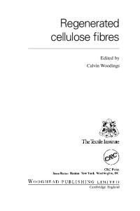
Figure 2.3.19 ID NMR spectra of CTAfTCM-d system: (a) ^H NMR; (b, c, d) ^H noise decoupled ^^C NMR; (b) carbonyl carbon region; (c) glucopyranose carbon region; (d) acetyl carbon region.'^
1
K ^
'
i E i
s^'^a
I
5^6 i r "•*
\ kL A . r a w J p* %
T rv ^ r-i
I I I
5 (^H)
Q. Q.
I I I
^
4 8/ppm
Figure 2.3.20 Schematic COSY spectrum of CTA/TCM-J (glucopyranose region). Filled and unfilled marks denote cross peaks and diapeaks, respectively.^^
2.3 DETERMINATION OF SUBSTITUENT GROUP
100
49
6/ppm
O^c)
^
Figure 2.3.21 Stacked plot for C-H COSY spectrum of CTA/TCM-j/^ a solvent (TCM-d) peak at 77 ppm is extraordinarily large and overlaps some of the CTA peaks, making further analysis on CTA spectrum impossible. In contrast, in the 2D spectrum, no peak of TCM-d, in which C-H coupling does not exist, is observed. Figure 2.3.22 shows a schematic C - H COSY 2D-spectrum constructed from Figure 2.3.21 and its cross section for the CTA/TCM-J system. In the figure, the projection of spectrum on the ^^C (horizontal) axis and the ^H (longitudinal) axis are also shown. Carbon peaks can be assigned based on assignment of proton peaks, using the C - H correlations shown in Figure 2.3.22 from the lower magnetic field to Ci, C4, C3, C5, C2, and C^ However, here C3 and C5 overlap and are inseparable. Figure 2.3.23 shows cross section spectra of long-range C-H COSY spectrum between the acetyl methyl proton and the acetyl carbonyl carbon in CTA/TCM-J. Three correlation peaks in these figures are peaks, originating from long-range scalar coupling of the carbonyl carbon of acetyl group and acetyl methyl proton. If we denote carbonyl carbon peaks from the lower magnetic field as a, b, and c, then the acetyl methyl proton peaks are assigned to a, c, and b.
o.S
I
fi
-X, 100 (13C)
80 6/ppm
60
Figure 2.3.22 Schematic C-H COSY spectrum of CTA/TCM-J (glucopyranose region).^^
2.
50
CHARACTERIZATION OF CELLULOSE DERIVATIVES
OH)
-1
I
I
I
I I
I
I
I
I
L
170 (^^C)
_L_L
169 6/ppm
Figure 2.3.23 Cross sections of long-range C-H COSY spectrum of CTA/TCM-d (acetyl carbonyl carbon region)." These relationships are in excellent agreement with the correlation obtained by the long-range selective spin decoupling method by Kowsaka et al}^ Using these results together with the assignment of the acetyl methyl proton peak chemically speculated by Goodlett et al.,^ carbonyl carbon peaks can be assigned from the lower magnetic field to Cg, C3, and C2, respectively. It is also expected that if long-range scalar coupling between the glucopyranose skeleton proton and carbonyl carbon could be observed, then carbonyl carbon peaks at C2, C3, and Cg positions could occur. However, a possible long-range coupling constant between the proton attached to glucopyranose carbon and carbonyl carbon (i.e. H^ proton and carbonyl carbon at C^ position) is actually too small to detect. In addition, in long-range C - H COSY measurements, the S/N ratio is significantly low due to the rapid transverse relaxation of magnetization of nuclei in CTA molecules. For this reason, we could not observe this kind of coupling for this polymer system. Similarly, we measured long-range COSY of protons in order to determine the correlation between the ring proton and the acetyl methyl proton, but failed due to the low S/N ratio. In the future, it may become possible to make a long-range measurement by (1) ^^C enrichment, (2) decrease in internal viscosity by lowering the polymer molecular weight, (3) 2D NMR by high magnetic field NMR apparatus, and (4) using other advanced 2D NMR techniques such as correlation spectroscopy via long-range coupling (COLOC).^^ From COSY and C - H COSY for the CTPJDMSO-de system, the almost comparable peak assignment was obtained for the CTAIDMSO-d^ system in the same manner as was carried out for CTA/TCM-J. Figure 2.3.24 shows a stacked plot of long-range C - H COSY (carbonyl carbon peak region) for CTPJDMSO-d^ system. The figure confirms the correlation between carbonyl carbons and acetyl methyl protons obtained by the long-range selective spin decoupling method by Kowsaka et al.^
2.3 DETERMINATION OF SUBSTITUENT GROUP
51
Figure 2.3.24 Stacked plot for long-range C-H COSY spectrum of CTA/TCM-J (acetyl carbonyl carbon region)/^ In summary, the reliability of peak assignment of ^H and ^^C NMR spectra for cellulose and its triacetate was undoubtedly strengthened by the use of 2D NMR. We demonstrated that overlapping peaks in ID NMR, whose existence could only be speculated from their intensity, were experimentally verified often from the splitting of peaks on 2D spectrum. With the use of 2D NMR, more complete and reliable calculations may be possible for almost all peaks in NMR spectra of not fully substituted cellulose derivatives with ((F)) ranging from 0.5 to 2.5, for which peak assignment was unfortunately impossible by ID spectrum alone due to the coexistence of various kinds of glucopyranose units (i.e. unsubstituted, mono-, di-, and trisubstituted units; see Section 2.4). 2.3.3
Sodium cellulose sulfate^^
As an extension of the previous sections, an attempt is made to evaluate ((/^)) as well as ((F)) for sulfate groups in sodium CS (NaCS) by ^H and ^^C NMR methods.^^ Experiments Purified cotton lint was hydrolyzed with 1.0 mol aq. sulfuric acid at 60 °C for 6 h to give a cellulose sample having a viscosity-average molecular weight, My = 0.9 X 10"^. NaCS was synthesized by reacting cellulose with sulfur trioxides dimethylformamide (DMF) complex at 10 °C according to the method proposed by Schweiger.^^ This was followed by the addition of sodium hydroxide. NaCS thus prepared was redissolved in water to give a solution of 5 g d l ~ \ dialyzed with purified water until the electroconductivity of the dialysate became below 1 X 10"^ £L~^ cm~\ and dried in vacuo. The NaCS sample had a viscosity average molecular weight. My = 15 X 10^, which was determined by putting the limiting viscosity number [ri\{= 544) in a 0.5 mol aq. NaCl solution at 25 °C into the Mark-Houwink-Sakurada equation: [r/] = 7.91 X 10"^ M^^^,^^ ((F)) was determined by chemical analysis^^ (method of gravimetric analysis by converting sulfuric group into barium sulfate following decomposition of NaCS with hydrochloric acid), and was found to be 1.96. The ^H and ^^C NMR spectra (100 MHz) of the NaCS solution in deuterium oxide (D2O) were obtained by a JOEL FX 100 Pulse-Fourier Transform NMR spectrometer at 37 °C.
52
2.
CHARACTERIZATION OF CELLULOSE DERIVATIVES
R = SOgNa
Figure 2.3.25 Possible conformation of glucopyranose units in sodium CS (((F)) = 2.0). Numbers denote positions of carbon atoms to which a nonsubstituted hydroxyl groups are attached, constituting the glucopyranose units.'^ Numbers in circles denote positions of carbon atoms, to which substituted hydroxyl groups are attached.'^ Figure 2.3.25 demonstrates all three differently sulfonated anhydroglucose units of NaCS with ((F)) = 2.00. Figure 2.3.26 shows ^^C NMR spectrum in D2O. Carbons at the C2-C5 positions yield complicated peak signals at 7 0 - 8 0 ppm, from which neither ((/2)) nor ((/3)) could be directly estimated. C^ carbon gave three peaks at 63.4, 61.2, and 60.8 ppm. Since the deshielding effect due to sulfate groups is expected to be almost equivalent to that of the acetyl group, the peak at 63.4 ppm could be attributed to the Ce carbon bearing the sulfate group. The peak signal at 60.8 ppm is considered a result of the unsubstituted C^ carbon. The peak at 61.2 ppm may be assigned to either Dionow
60ppm Figure 2.3.26 '^C NMR spectrum of NaCS (((F)) = 1.96) in deuterium oxide. Numbers and symbols are the same as described in Figure 2.3.25.^^
2.3 DETERMINATION OF SUBSTITUENT GROUP
53
the unsubstituted €5 carbon (Hypothesis A) or the C^ carbon bearing free sulfate group (-OSO3H) (Hypothesis B). The ((/6)) value differs in regard to the assignment of the 61.2 ppm peak signal, which was found to be 0.34 for Hypothesis A and 0.44 for Hypothesis B from the area under peaks. In Table 2.3.3, the chemical shift and assignment of the peaks of ^^C NMR spectrum are presented. Three peaks at 103.1, 102.7, and 99.4 ppm are assigned to the Ci carbon, which was employed by Wu"^ for estimating ((/2)) and ((/3)) of the nitrate group. However, in this case, these peaks cannot be used for estimating ((/2)) and ((/3)) due to insufficient knowledge about the shielding effect of sulfate groups in the C2 and C3 positions. Of course, the integrated intensity of the Ci carbon region was nearly equal to that of the C^ carbon region. Figure 2.3.27 shows the corresponding ^H NMR spectrum of NaCS solution in D2O. OH groups from NaCS were all converted into OD groups. Peak assignment was performed by a mutual comparison of peak areas and a comparison of the spectrum with that of cellulose acetate. ^^ The proton signal at the C3 position, which was sulfated, appears at the lowest magnetic field strength (4.97 ppm). A side band from HOD may be included in Peaks 3 and 1. In Table 2.3.3, the chemical shifts, assignments, and intensities of the peaks are shown together. Thus, ((/2)), ((/3)), and ((/6)) can be accurately evaluated from ^H NMR spectrum alone within an accuracy of ±0.030, 0.035, and 0.012, respectively, by the following equations. « / 2 » = ^
(2-3.2)
«/3» = 4 ^
(2.3.3)
«/6» = ^
(2.3.4)
Table 2.3.3 Chemical shift and assignment of the peaks in ^^C NMR spectrum of sodium CS^^ ((F)) by chemical analysis 1.96
Chemical shift/ppm Ci
C2-C5
Ce
103.1, 102.7, 99.3
79.2, 78.0 75.6, 74.7, 73.6, 73.2
63.4, 61.2, 60.8
54
2.
CHARACTERIZATION OF CELLULOSE DERIVATIVES I HOD 3,4,6
Figure 2.3.27 ^H NMR spectrum of NaCS (((F)) -- L96) in deuterium oxide. symbols are the same as described in Figure 2.3.25.
Numbers and
where Z^, I2,13, I^^ /s, and 4 are the integrated peak intensities at 4.97, 4.83, 4.56, 4.39, 4 . 0 - 3 . 5 , and 3.42 ppm, respectively. Equation (2.3.4) was derived assuming that the proton directly attached to the substituted €5 position is not contaminated in the integrated peak intensity I^. The validity of this assumption is confirmed by 7/3
(2.3.5)
= 1.00
Putting the data from Table 2.3.4 into eqs. (2.3.2)-(2.3.4) gives ((/2)) = 1.00, {{f^}} = 0.61, and {{f^,}) = 0.34. The latter value (0.34) is in good agreement with that (0.34) evaluated with Hypothesis A. This confirms the validity of the assignments proposed for the ^^C NMR spectrum. In addition, from the ((/^)) data by ^H NMR, we obtain ((F)) = 1.95, which agrees well with that of the chemical analysis. Table 2.3.4 Chemical shift, assignment, integrated peak intensity, and ((/^)) of ^H NMR spectrum for sodium cellulose sulfate in deuterium oxide'^ Chemical shift Assignment 8 (ppm)
m) Chemical analysis
1.96
Peak intensity ((/^))
'HNMR
1.95
4.97 4.83 4.56 4.39 4.0-3.5 3.42
H3 Proton^ H2 Proton^ Hi Proton H6 Proton^ H3, H6, H4 protons H5 Proton
/i = 16.2 12 = 26.7 13 = 26.7 14 = 18.0 /5 = 720 /i = 26.7
"Signal of protons attached to C/, (A: = 2, 3, and 6) position bearing a sulfategroup.
0.61 1.00 0.34(0.34)^^C NMR
55
2.3 DETERMINATION OF SUBSTITUENT GROUP
The Ci proton signals in ^H NMR spectra possibly overlap with the proton signals of the Ce position bearing sulfate group. This makes the evaluation of ((/6)) by ^H NMR analysis difficult. Even in this case, ((/^)) can be determined by the following procedure. (1) determination of ((F)) by chemical analysis (2) determination of ((/2)) and ((/3)) using eqs. (2.3.2) and (2.3.3) (3) determination of ((/g)) by «/6» = m
- («/2» + «/3»)
(2.3.6)
The reactivity of hydroxyl groups at the C2, C3, and C^ positions of cellulose with the SO3-DMF complex decreased in the following order: C2 > C3 > Ce- If the hydrolysis reactions of NaCS are assumed to be the reverse of the order mentioned above, then the hydrolysis of the substituent at C2 is the lowest. This clearly contradicts the fact that the reactivity of 0-acetyl groups in C A with hydrochloric acid, previously evaluated, is of the order: C2 > C3 > €5. This means that the reactivity of hydroxyl or substituents of cellulose or its derivatives cannot be primarily predicted according to the position alone. 2.3.4 CA whose acetyl groups are located only at Ce position (i.e. 6-O-acetyl cellulose or CA with ((fg)) ^ 0 and ((fz)) = ((fs)) = Of^ It is not sufficient to characterize CA in terms of ((F)), ((/^)), and ^fimJ) in order to establish the correlations between the molecular structure and their physical and physiological properties. Generally, any CA prepared by conventional methods has wide
HCA01
HCA02
J
J
J
HCA03
-^'
HCA04
J
HCA05
J\- j _
A
-^^-^
I i A
_l
I
L_ J
L
170169 102 80 76 72 64 60
ppm 2120
Figure 2.3.28 ^^C NMR spectra of 6-O-acetyl cellulose in DMSO-^.
2.
56
CHARACTERIZATION OF CELLULOSE DERIVATIVES
variation with ((A)). If CA, whose acetyl group is located at specific carbon position alone, is available, then the polymer is expected to contribute significantly to establishment of structure-properties relationships. Recently, Yasuda and Kamide 21 synthesized 6-0-acetyl cellulose by homogeneous acetylation and subsequent homo geneous deacetylation or their repetition. 6-0-acetyl
cellulose
Step 1: Cellulose was acetylated at 30 °C in dimethylacetoamide (DMAc)/LiCl mixture (92 and 8 wt/wt) using pyridine and acetic anhydride^^ to give CA whose distribution of acetyl group is {(fe)) » ((A)) - ((/s)). Step 2: CA thus prepared was deacetylated at 30 °C in DMSO using 80 wt% aq. solution of hydrazine monohydrate. The detailed reaction conditions were carefully chosen so as to yield CA whose acetyl groups are preferentially located only at the C^ position (i.e. W) ^ 0, ((/2)) = {{/,)} = 0).
I
I
•
•
I
•
•
•
I
'
•
•
•
•
170
—I—I—I—I—I—I—I—I—I—I—I—I—I
170
I
'
I
•
• — I —
169
I
I
I—I—I—I—
169
Figure 2.3.29 ^ "^C NMR spectra of the carbonyl carbon of CA (a) two-step method ((F)) = 2.46, (b) two-step method ((F)) = 0.54, (c) 6-O-acetyl cellulose ((F)) •- 0.62, (d) 2,3-O-acetyl cellulose
2.3
DETERMINATION OF SUBSTITUENT GROUP
57
Table 2.3.5 ((A)) of CA samples, prepared by homogenous acetylation and subsequent homogenous deacetylation and, if necessary, the repetition of these for adequate time (n) Sample code
HCAOl HCA02 HCA03 HCA04 HCA05
n
1 1 2 2 3
((/s))
((/2))
Average
((/6))
A
B
A
B
A
B
C
0.0 0.0 0.0 0.0 0.0
0.0 0.0 0.0 0.0 0.0
0.0 0.0 0.0 0.0 0.0
0.0 0.0 0.0 0.0 0.0
0.28 0.35 0.42 0.53 0.62
0.27 0.33 0.42 0.51 0.62
0.30 0.37 0.42 0.52 0.62
0.28 0.35 0.42 0.52 0.62
A, carbonyl carbon; B, skeletal carbon; C, methyl carbon. Steps 1 and 2 were repeated in order to prepare CA with relatively higher ((F)). Figure 2.3.28 shows ^^C NMR spectra of CA samples, whose acetyl groups are located only at the Ce position in DMS0-J6- The peaks at ca. 170, 6 0 - 1 0 5 , and 2 0 p p m are assigned to the carbonyl carbon,^^ the skeleton carbon, ^^ and the methyl carbon of acetyl group,^^ respectively. Figure 2.3.29 shows ^^C NMR spectra of the carbonyl carbon of several CA samples in DMS0-J6. Kowsaka et al. gave a very detailed assignment of this region as shown in Table 2.3.6 Peak assignments in ^^C NMR spectra of cellulose acetate, in which all acetyl groups are located at C^ position Peak number
Peak position d ppm (in DMSO)
Assignment
1 2 3 4 5 6 7 8 9 10 11 12 13 14 15 16 17 18 19 20
170.04 170.00 102.69 102.47 102.13 79.95 79.44 75.05 74.98 74.92 74.82 74.56 74.19 73.20 73.11 72.86 72.03 63.15 60.56 20.42
Acetylcarbonyl(/ooo-/ooi, /ooi -/ooo) Acetylcarbonyl(/ooi -/ooi) Ci (/ooo-fooo^/ooo-Zooi or/oo 1-/000) Ci (/000-/001 or/oo 1-/000) Ci (/oo 1-/001) C4 (/ooo -/ooo^ /ooo -/oo 1»/oo 1 -/ooo) C4 (/oo 1-/001) C5 (/ooo) C3 C3
C3 (/ooo or/ooo-/ooo) C3 C3 (/oo 1-/001)
C2 (/ooo-/ooo) C2 C2 (/oo 1-/001)
C5 (/ooi) C6 (/ooi)
C6 (/ooo) Acetylmethyl
58
2.
PV
DMAc/LiCI
tritylchloride /pyridine cellulose
CHARACTERIZATION OF CELLULOSE DERIVATIVES
, ^ S ^ ^ ^
Py^'^'"®
/ i ^ o - ^ o ^'=®*''= ^ o X ^ ^ anhydride 6-0-tritylcellulose
Figure 2.3.30
_. V^^_.
dichloro -methane
^ r , / ^ o - T o MUL HCLgas gas °^ir^,.^ 2,3-0-acetyl6-0-tritylcellulose
pn OAc
OAc
2,3-O-acetylcellulose
Schema of synthesis of 2,3-0-acetyl cellulose; *1: see Ref. 24; *2: see Ref. 25.
Figure 2.3.29a and b. The peak of Figure 2.3.29c is quite sharp, although it contains a shoulder (see also Figure 2.3.28). The CA sample in Figure 2.3.29d apparently has ((/6)) = 0. Analysis on the carbonyl carbon peaks (peaks 1 and 2 in Figure 2.3.28) and skeleton carbon peaks (peaks 18 and 19 in Figure 2.3.28) allows us to estimate ((/^)) (k = 2, 3, and 6). The results are summarized in Table 2.3.5. Inspection of Table 2.3.5 leads us to the conclusion that CA samples synthesized by homogeneous acetylation and subsequent homogeneous deacetylation (i.e. two homogeneous steps) have, without exception, ((/2)) = ((/3)) = 0. In addition to these methods, ((/6)) can be determined from the acetyl methyl carbon peak (Peak 20; Yasuda and Kamide,^^ as included in Table 2.3.5). Three methods gave almost the same ((/6)) within ± 0 to ± 0.02. CA, whose acetyl groups are solely located on C^ position, is very helpful to reinforce the assignment of ^^C NMR spectra of CA. Table 2.3.6 collates the peak assignments. 2,3-0-acetyl
cellulose (CA whose acetyl groups are not located at
exposition)
2,3-0-acetyl cellulose was synthesized via 6-O-tritylcellulose and 2,3-di-0-acetyl-6-0tritylcellulose from cellulose. A scheme of the synthesis is shown in Figure 2.3.30. ^^C NMR spectra of carbonyl carbon of this sample (CA with (^f^)) = 0) is included in Figure 2.3.29d). REFERENCES
1. 2. 3. 4. 5. 6. 7. 8. 9. 10. 11. 12. 13. 14.
TS Gardner and CB Purves, /. Am. Chem. Soc, 1942, 64, 1539. CJ Malm, JJ Tanghe and BC Laird, /. Am. Chem. Soc, 1950, 72, 2674. W Goodlett, JT Dougherty and HW Patton, J. Polym. Sci. A-1, 1971, 9, 155. TK Wu, Macromolecules, 1980, 13, 74. See, for example, K Kamide and K Okajima. Polym. J., 1981, 13, 127. N Shiraishi, T Katayama and T Yokota, Cell. Chem. TechnoL, 1978, 12, 429. T Miyamoto, Y Sato, T Shibata, H Inagaki and M Tanahashi, J. Polym. Sci. Polym., Chem., Ed., 1984, 22, 2363. K Kowsaka, K Okajima and K Kamide, Polym. J., 1986, 18, 843. K Kamide and M Saito, Eur. Polym. J., 1984, 20, 903. K Kamide, K Okajima, K Kowsaka and T Matsui, Polym. J., 1987, 19, 1405. K Kowsaka, K Okajima and K Kamide, Polym. J., 1988, 20, 1091. D Gagnaire, D Mancier and M Vincendon, J. Polym. Sci. Polym. Chem. Ed., 1980, 18, 13. K Kamide, K Kowsaka and K Okajima, Polym. J., 1987, 19, 231. R Nardin and M Vincendon, Macromolecules, 1986, 19, 2452.
2.4
MOLAR FRACTION OF EIGHT KINDS OF GLUCOPYRANOSE UNITS
59
15. See, for example, E Breitmeier and W Voelter, ^^C NMR Spectroscopy, 3rd Edn., Verlag Chemie, Weinheim, New York, 1986. 16. K Kamide and K Okajima, Polym. /., 1981, 13, 163. 17. FG Schweiger, Carbohydr. Res., 1942, 21, 219. 18. K Kishino, T Kawai, T Nose, M Saito and K Kamide, Eur. Polym. /., 1981, 17, 623. 19. H Friebolin, G Keilich and E Siefert, Angew. Chem. Int. Ed., 1969, 8, 766. 20. K Kamide and M Saito, Macromol. Symp., 1994, 83, 233. 21. K Yasuda and K Kamide, unpublished results. 22. See, for example, T Miyamoto, Y Sato, T Shibata, M Tanahashi and H Inagaki, /. Polym. ScL, Polym. Chem. Ed., 1985, 23, 1373. 23. K Kowsaka, K Okajima and K Kamide, Polym. J., 1988, 20, 827. 24. S Takahashi, T Fujimoto, BM Barua and T Miyamoto, /. Polym. ScL, A. Polym. Chem., 36, 952. 25. T Kondo and DG Gray, Carbohydr. Res., 1991, 220, 173.
2.4
MOLAR FRACTION OF EIGHT KINDS OF UNSUBSTITUTED AND PARTIALLY OR FULLY SUBSTITUTED GLUCOPYRANOSE UNITS (((f,^„)))^
When we see the possible substituted glucopyranose units of cellulose derivatives, there are eight kinds of unsubstituted and partially or fully substituted glucopyranose units
^H20RQ
R=-C0CH3
0
RO ^'^'^ MDHgOR
trisubstituted J^20R
/^^ORQ
^°V^ "°V^° - \ ^ ° 2 3— «fl10>>
©
2,6—
©
^^HgOR
^wCHsOR
Ho\x^V^O ®, O ^ 2— «f^00>>
RoV^^>>^0 ® OH o— «fOio»
HO,^/^^0 ® OH
3,6— «f011>> ; disubstituted
® --^^SORQ HoV'^Tsi^O @ OH b— «f001''> ; monosubstituted
unsubstituted
«fooo>> Figure 2.4.1 Substituted and unsubstituted glucopyranose units in CA molecules^: ^fimJ} represents molecular fraction of the units.
60
2. CHARACTERIZATION OF CELLULOSE DERIVATIVES
as shown in Figure 2.4.1. These are single trisubstituted, three disubstituted, three monosubstituted, and one unsubstituted glucopyranose units. Molar fractions of these glucopyranose units ((//^„)), defined in detail below, are an effective measure of the distribution of the substituent group within a glucopyranose unit, enabling us to judge whether the reaction is homogeneous or not. In addition, an accurate evaluation of these fractions is important in order to understand, on a molecular basis, the solubility of cellulose derivatives against various solvents and the physiological properties. Since the 1950s, the separation and quantitative determination of tri-, di-, monosubstituted, and unsubstituted glucopyranose units have been exclusively performed by applying distillation and chromatographic techniques to chemically decomposed cellulose derivatives, particularly sodium cellulose xanthate.^ However, the decomposition of CD molecules into glucose units is extremely difficult without desubstituting reactions, in spite of the numerous attempts to prevent such reactions. In fact, experimental results reported about ((//,„„» of cellulose xanthate differ depending on the researchers who carried them out. However, the conversion of the xanthate group into a more stable form involves very complicated chemical reactions.^ Methods have been proposed by Wu,^ and Clark and Stephenson^ for estimating molar fractions of 2,3,6-tri-, 2,6-di-, 3,6-di-, and 6-mono substituted glucopyranose units of cellulose nitrates, whose C^ position was fully substituted (i.e. ((/g)) = 1) from their ^^C NMR spectra. However, their methods cannot be applied to CN whose hydroxyl group at the C^ position is not fully substituted. 2.4.1
Cellulose acetate^
This section assigns all peaks in the carbonyl carbon region of ^^C NMR spectra of CA and provides a firm basis for estimating ((/^)) and molar fractions of eight kinds of glucopyranose units of CA by NMR alone. Sample preparation A CTA whole polymer with ((/^)) = 2.92 (sample code CA-0) and nine incompletely substituted CA samples, prepared by acid hydrolysis of sample CA-0 in acetic acid (sample code CA-1 to CA-9), were used. The procedures are described in detail elsewhere.^'^ Table 2.4.1 collects the average molecular weight M^ of sample code CA-0 and -1, determined by light scattering in DMAc, and the viscosity average molecular weight My of sample code CA-2 to CA-7, determined from the limiting viscosity number in DMAc solution.^"^ NMR measurement Proton noise decoupled ^^C NMR (^^C{^H} NMR) spectra of these CA solutions in deuterated dimethylsulfoxide (DMSO-Je) were recorded on an FX-200 FT-NMR spectrometer (JEOL, Japan) at a resonance frequency of 50.18 MHz at 90 °C. The detailed operating conditions were almost the same as those reported in Section 2.4.2. TMS was the internal reference. Integrated peak intensity was determined from an
2.4 MOLAR FRACTION OF EIGHT KINDS OF GLUCOPYRANOSE UNITS
61
Table 2.4.1 Degree of substitution, weight, and viscosity average molecular weight and peak chemical shift in carbonyl region of CAs^ Sample code
m
Mw,
CA-0
2.92
2.32^
169.94
CA-1
2.46
1.05^
CA-2
1.75
0.82^
CA-3
1.23
0.80^
CA-4
1.06
0.64^
170.02, 169.95, 169.82 170.04, 169.97, 169.83 170.06, 170.00, 169.97, (169.85) 170.04, 169.96, 169.87
CA-5
0.95
0.47^
170.00, 168.87
CA-6
0.77
0.36^
170.04, (168.88)
CA-7
0.69
0.33^
CA-8
0.54
—
CA-9
0.43
170.04, 169.88, (168.89) 170.02, 169.97, (169.90) 170.04, (169.99), 169.90, 169.78
Chemical shift/ppm (±0.02 ppm)
(Mv)/10^
'
169.40, (169.17), 169.11 169.41, 169.11 169.43, 169.17, 169.14, 169.11 (169.61), 169.45, 169.21, 169.16 169.58, 169.46, 169.34, 169.22, 169.10 169.61, 169.48, 169.36, 169.22 169.59, 169.47, 169.36, 169.18 169.61, 169.46, 169.34 169.59, (169.43), 169.34, 169.09 169.61, 169.34, (169.10)
168.93, 168.78 168.91, 168.78, 168.73 168.93, 168.80 168.92, 168.79, (168.72) 168.92, 168.77 168.93, 168.87 168.93, 168.75 168.93, (168.71) 168.92, 168.79 168.94
""Mw, from light scattering. ^Mv, from [ry] in DMAC at 25 °C. integral curve. ((F)) was evaluated from the integrated intensity ratio of peaks in acetyl methyl carbon region (20-22 ppm) and peaks in Ci carbon region (91-105 ppm). The second column of Table 2.4.1 show^s the ((F)) of these CA samples. Figure 2.4.2a-j shovv^s the carbonyl carbon region of ^^C{ ^H} NMR spectra of samples CA-0 to 9 in DMSO-(i6. These spectra were recorded at a spectral width of 1 kHz (4096 data points) in order to attain high digital resolution. The chemical shift from TMS as an internal reference was determined from the spectra obtained independently at a spectral width of 10 kHz (8192 data points). The digital resolution of these spectra was estimated to be approximately 0.01 ppm and the relative error of chemical shifts was less than 0.02 ppm. In the spectrum of sample code CA-0 (((F)) = 2.92) in Figure 2.4.2a, three main peaks were observed, as reported in a previous paper,^ originating from trisubstituted glucopyranose unit, and these peaks are assigned, from the lower magnetic field, to three carbonyl carbons at C^, C3, and C2 positions, respectively. In the same spectrum, small peaks or shoulders, observed at 169.4,169.2, and 168.9 ppm (as denoted by arrows in the figure), may possibly have originated from disubstituted glucopyranose units. In the spectrum of sample CA-9 (((F)) = 0.43) in Figure 2.4.2J, three peaks (170.0, 169.6, and 168.9 ppm) due to three monosubstituted glucopyranose units, are observed. In addition, a group of small peaks (as denoted by arrows in the figure), considered to
62
2. CHARACTERIZATION OF CELLULOSE DERIVATIVES
(a) (b) (c) (d) (e) 1 . .
J\
ij
Li . ^A^-^v.
JU\A. S^ . A>{v Ay^V 170
(f) yV^w-wA.
'!lJ}y^}^
^JiUwJL. 170
169 ^/ppm
d> d> d>
O
^
ON
d d
O
d d o (^ d d
I
O '
(O (D d> d>
o
o
o en ^ vo o o o o
—
m o CO o (N d> d>
o o o o
2)
(2.4.16)
«/ioi» = Ai
(for cellulose acetate with «F)) < 2)
(2.4.17)
«/oii» = h+h=h+h+r9 «/ioo» = hi
(for cellulose acetate with {{F}) < 2)
(2.4.18) (2.4.19)
«/oio)) = /6
(2.4.20)
«/ooi» = /i
(2.4.21)
The peaks in ^ ^ C { ' H } N M R spectra of CA samples (except for CA-0) are quite broad indeed and overlap significantly, as shown in Figure 2.4.2. Thus, an accurate evaluation of ((/ten)) for CA is quite difficult.
68
2. CHARACTERIZATION OF CELLULOSE DERIVATIVES
Since for the sample code CA-8 peaks 6, 11, and 12 are separately observed without overlapping with other peaks, ((/oio)), ((/loo))? ^^^ ((/loi)) for the sample can be evaluated using the /„ data of these peaks (Table 2.4.3) from eqs. (2.4.17), (2.4.19), and (2.4.20), respectively. The fraction ((/no)) for the sample can also be determined from eq. (2.4.14) using data on /13 + /14 in Table 2.4.3 and assuming ((/m)) = 0, because (1) Peaks 13 and 14 overlap with each other, but not with other peaks, enabling an estimate of/13 H- 114 and (2) ((F)) for this sample is low (0.54). ((/on)) for the sample can also be evaluated using data on /y + /g + Ig from eq. (2.4.18), in the same manner. In addition, for this CA sample. Peak 1 significantly overlaps with Peaks 2, 3, 4, and 5. Thus, ((/ooi)) cannot be simply estimated from eq. (2.4.21) using /1 data. An alternative way of estimating ((/ooi)) is given by the equation: ((/ooi)) = f^Ij - ((/loi)) - ((/oil)) - ((/ill))
(2.4.22)
A combination of eqs. (2.4.5) and (2.4.10) leads to eq. (2.4.22). Neglecting ((/m)) in eq. (2.4.22) for sample CA-8, ((/ooi)) can be estimated roughly from ((/loi)) and ((/on)) data previously determined by eqs. (2.4.16) and (2.4.18). Equation (2.4.6) can be rearranged as follows: = 1 -(> + + ()+>
^V^'^^o
"^SS'^^o
H O ^ k f ' ' ^ ' > \ ^ 0 RoXf-^^^iv^O (3)
OR
2«f-IOo» ®Qi_i OH
^^^V^^iS^ ^f
^^
0)
OH
3«f010>^
3,6«^011>^ ; disubstituted
-^S^^^^o HoX^-^^^I^O OH
6«^001>> ; monosubstituted
; unsubstituted
Figure 2.4.4 Substituted and unsubstituted glucopyranose units in NaCS molecules: ^^ UmJ) represents molar fraction of the units.
72
2.
CHARACTERIZATION OF CELLULOSE DERIVATIVES
J_L
I
I I I
5/ppm
Figure 2.4.5 ^^C{^H} NMR spectra of NaCS samples in D2O solution using WEFY technique: (a) sample DS-1; (b) sample DSH-1; (c) sample HBH-l/^ might be due to a shorter pulse interval, applied for WEFT here, than the most adequate pulse interval ('null point') and the resonance is assigned to HDO proton. The peak appearing at 3.36 ppm in Figure 2.4.5c is responsible for methanol, which is introduced as a contaminant during the preparation of NaCS, and this peak was ignored in further analysis. For DS-1, ^H peaks are observed in the chemical shift (8) range of 3.6-5.0 ppm. On the other hand, for DSH-1 and HBH^-1, ^H peaks are observed in the chemical shift range of 3.3-4.7 ppm. Taking the estimated reading error of 8 (0.02 ppm) into account, 10 ^H peaks were detected besides the HDO peak. The 8 values of all the peaks detected for each NaCS sample are listed in Table 2.4.6. The peaks appearing around 4.4 and 4.6 ppm in Figure 2.4.5b and c are triplet peaks split by vicinal coupling. Therefore, the 8 values at the central peaks are employed in the table. Note that, judging from the number of peaks observed and their 8 values, the sample DSH-1 is similar to that reported for NaCS with ((F)) = 1.96, synthesized by Kamide and Okajima.^^ Figure 2.4.6 shows the ^^C{^H} NMR spectra of DS-1 (a), DSH-1 (b), and HBH'-l (c). The spectra of DSH-1 and HBH^-1 are similar to each other, except for nine small sharp peaks, marked by arrows in Figure 2.4.6c, which probably originated from
2.4
MOLAR FRACTION OF EIGHT KINDS OF GLUCOPYRANOSE UNITS
73
Table 2.4.6 Chemical shifts 8 of proton peaks of NaCS sample in D20^^ Peak no.
8 (ppm) DS-1
1 2 3 4 5 6 7 8 9 10 11
DSH-1
HBH'-l
4.58 4.43 4.32
4.57 4.42 4.30
4.02 3.96 3.85 3.68 3.38
4.02 3.96 3.84 3.67
4.93 4.70 4.41 4.28 4.18 3.84 3.66 3.39
contaminants such as cellulosic oligomers produced as a by-product during synthesis of HBH^-1. Sixteen peaks in total were observed and their 8 values are indicated in Table 2.4.7. Table 2.4.8 gives the chemical shifts and peak assignments of ^H and ^^C NMR peaks for cellulose/NaOD at 20 °C, which was cited from Figures 2.3.16 and 2.3.18. Here, the assignments for the ^^C peaks at 81.8 and 78.2 ppm are made with reference to Nardin and Vincendon's study/^ which was carried out for the cellulose/dimethyl
5/ppm
Figure 2.4.6 ^^C{^H} NMR spectra of NaCS samples in D2O solution:^^ (a) sample DS-1; (b) sample DSH-1; (c) sample HBH'-l.
74
2.
CHARACTERIZATION OF CELLULOSE DERIVATIVES Table 2.4.7
Chemical shifts 8 of proton peaks of NaCS sample in D20^^ Peak no.
8 (ppm) DS-1
1 2 3 4 5 6 7 8
104.8 103.4 102.9 84.5 82.4
81.2
Peak no. DSH-1 104.8 104.6 7 7
84.3 7 81.7 81.3
8 (ppm) DSH-1
HBH'-l
DS-1
104.8 104.6 7 7
_
80.6
80.1 77.5 (76.8*) 75.8 75.5 (74.3?) 69.2
-
-
77.5 76.8 75.8 75.5 (74.3?) 69.2 63.0
77.5 76.8 75.8 75.5 (74.3?) 69.2 63.0
7 81.7 81.3
9 10 11 12 13 14 15 16
-
HBH'-l 80.6
?, not clearly detected; -, not detected; *, included in peak 11; (74.37), detected but not clear to arise from AHG units polymer. acetamide/lithium chloride system. A comparison of Tables 2.4.6 and 2.4.7 with Table 2.4.8 shows that DSH-1 and HBH^-1 have NMR peaks at almost the same positions as those observed for cellulose, but DS-1 has numerous peaks besides those observed for cellulose. This suggests that DS-1 is highly substituted. Figure 2.4.7 shows the contour plot of ^H COSY (power spectrum) of DS-1 with a projection on the horizontal axis. The projection spectrum shown in Figure 2.4.7 apparently has a higher resolution compared with the spectrum shown in Figure 2.4.5a, but a small peak (peak 10) at 3.66 ppm is suppressed. This might be due to the application of a trapezoidal window function to the observed free induction decay signal before Fourier transformation on the COSY measurement. The peaks, observed at 4.92 (doublet), 4.68 (triplet), 4.42 (triplet?), 4.14 (triplet), and 3.88 ppm (doublet) on the projection correspond to Numbers 1,2,4,6, and 9 peaks in Table 2.4.6, respectively. The peak at 4.92 ppm shows Table 2.4.8 Proton and carbon chemical shifts 8 of cellulose in aq. NaOD collected from Figures 4 and 6 in Ref. 16 Observing nucleus 'H
"C
8 (ppm) 4.49 3.95 3.80 3.57 3.29 106.7 81.8 78.2 76.8 63.5
Assignment Hi H6 H6
Hg, H4, H5 H2 Ci C4
C3,C5 C2
Ce
2.4 MOLAR FRACTION OF EIGHT KINDS OF GLUCOPYRANOSE UNITS
75
Figure 2.4.7 Homogate decouple proton COSY spectrum of NaCS (sample DA-1)/^ only one cross peak in the contour plot in Figure 2.4.7 and is attributed to Hi proton. The appearance of the cross peak at 4.42 ppm, shown as H1-H2 in Figure 2.4.7, enables us to attribute this peak to H2 proton. In a similar manner, H3, H4, H5 proton peaks can be assigned and the final assignments attained, excluding HDD proton peak region, are given on the projection spectrum, that is. Hi, H3, H2, H4, and H5 proton peaks from the lower magnetic field. Figure 2.4.8 shows the contour plot of CH-COSY (power spectrum) for DS-1 with projection spectra on the horizontal (^^C) and longitudinal (^H) axes. Six peaks, observed at 103.5, 81.2, 80.1, 77.5, 76.0, and 69.6 ppm on the ^^C projection spectrum, correspond to Numbers 3, 8, 10 (and 9), 11, 13 (and 14), and 15 peaks, respectively, in Table 2.4.7. The peaks assigned in Figure 2.4.7 are also observed in the ^H projection spectrum.
I I I I I I I I I 1.1 I 11 I I I I r r I I I I I I I 11 I I I I I I I I I I M I
100
^, 5/ppm
80
Figure 2.4.8 CH-COSY spectrum of NaCS (sample DS-1).^
76
2. CHARACTERIZATION OF CELLULOSE DERIVATIVES
The contour plot revealed that the ^^C peak at 103.5 ppm was correlated with the ^H peak at 4.93 ppm, assigning this ^^C peak to Ci carbon. In the same manner, three ^^C peaks at 81.2, 77.5, and 76.0 ppm were assigned to C3, C4, and C5 carbons, respectively. The ^H peak at 4.42 ppm (H2 proton) is correlated with two ^^C peaks at 80.1 and 69.6 ppm and, therefore, the peak at 4.42 ppm is expected to be an overlapping peak of H2 proton and another proton. The ^^C peak at 69.6 ppm is assigned to C^ carbon because the €5 carbon peak is, without exception, observed in the highest magnetic field in the spectra of cellulose,^^ cellulose acetate,^^ CN,"^ and CX.^ This leads to the conclusion that the ^H peak at 4.42 ppm originates from H2 and H6 (and H^) protons. Note that there are two magnetically nonequivalent H6 protons, H6 and H^. The difference between 8 values of ^H and ^^C peaks for DS-1 (cf. Figures 2.4.7 and 2.4.8) and those for cellulose (cf. Table 2.4.8) are summarized as follows: (1) the peaks due to H2, H3, and H6 protons for DS-1 appear in the lower magnetic field by 0.6-1.1 ppm than those of cellulose, (2) C2, C3, and C6 carbon peaks for DS-1 substantially shifted to a lower magnetic field (3.0-6.0 ppm), compared with the corresponding carbon peaks for cellulose, (3) hardly any of the 8 values of ^H and ^^C peaks for DS-1 coincide with those of cellulose. These facts suggest that almost all NMR peaks for DS-1 should appear as a result of the almost complete substitution of three hydroxyl groups at C2, C3, and C^ positions. Therefore, almost all peaks observed in Figures 2.4.7 and 2.4.8 originate mainly from the trisubstituted AHG unit although there are some peaks (84.0, 82.4, and 75.2 ppm) without a detectable cross peak on the CH-COSY spectra. Figure 2.4.9 shows ^H COSY of HBH^-1. The spectrum is quite similar to that for cellulose/NaOD system,^^ suggesting that ((F)) of this polymer is very low. The following assignments are easily made Hi, 4.57 ppm; H6, 3.99 ppm (doublet); H6, 3.84 ppm; (H3, H4, H5), 3.67 ppm; H2, 3.38 ppm. Besides these peaks, there remain three unassigned
/ ix Figure 2.4.9 Homogate decoupled proton COSY spectrum of NaCS (sample HMH^-1)
12
2.4 MOLAR FRACTION OF EIGHT KINDS OF GLUCOPYRANOSE UNITS
77
peaks at 5.22, 4.4, and 4.3 ppm, and the full assignment is not possible by ^H COSY alone. Figure 2.4.10 shows CH-COSY of HBH'-l. On the basis of ^H peak assignment given in Figure 2.4.9, the following ^^C peak assignment is made: 104.8 ppm, Cf, 75.8 ppm, C2; 63.0 ppm, C6. Three ^^C peaks (81.3, 77.5, and 76.8 ppm) are correlated with a (H3, H4, H5) proton peak (3.67 ppm) and then, these ^^C peaks should be assigned to either C3, C4 or C5 carbons. Although these three peaks are cannot be assigned completely only from Figure 2.4.10, the peak at 81.3 ppm can be attributed to C4 carbon from the assignment in Table 2.4.7. The remaining two peaks at 77.5 and 76.8 ppm were assigned to C5 and C3, respectively, with reference to Nardin and Vincendon's assignment^^ carried out for cellulose/dimethylacetamide/lithium chloride system and to Gagnaire et aUs assignment^^ on low molecular weight cellulose in dimethyl sulfoxide. Since 8 values of ^H and ^^C peaks assigned above for HBH^-1 are confirmed to be almost the same as those for cellulose, almost all these peaks should originate from unsubstituted AHG units. Inspection of two cross peaks (see Figure 2.4.10) indicates that the ^^C peak at 69.2 ppm is due to 6-mono-substituted AHG unit because there are no cross peaks due to substituted C2-H2 and substituted C3-H3 in the dotted circle region, as shown in Figure 2.4.10, and because the total DS of HBH^-1 is quite low. The peaks at 81.7 and 80.6 are correlated with ^H peak around 3.67 ppm and therefore attributable to either C3, C4 or C5 carbon. The peak at 75.5 ppm is correlated with ^H peak around 3.84 ppm. 2D NMR spectra shown in Figures 2.4.7-2.4.10 enables us to assign the following peaks: (1) all ^^C and ^H peaks for 2,3,6-trisubstituted AHG unit (Ci, 103.4 ppm; C2, 80.1 ppm; C3, 81.3 ppm; C4, 77.5 ppm; C5, 75.8 (75.5) ppm; Ce, 69.2 ppm; Hi, 4.93 ppm; H2, 4.42 ppm; H3, 4.70 ppm; H4, 4.18 ppm; H5, 3.84 ppm; H6, 4.42 ppm); (2) all ^^C and ^H peaks for unsubstituted AHG unit (Ci, 104.8 ppm; C2, 75.8 (75.5) ppm; C3,76.8 ppm; C4, 81.3 ppm; C5, 77.5 ppm; Ce, 63.0 ppm; Hi, 4.58 ppm; H2, 3.39 ppm; H3, 3.67 ppm; H4, 3.67 ppm; H5, 3.67 ppm; H6, 3.96 and 3.84 ppm). Table 2.4.9 gives the observed 8 values of ^H peaks for the 2,3,6-trisubstituted AHG unit and unsubstituted AHG unit. Denoting the carbon atom directly attached to the proton in question as the neighboring carbon to CQ, as C/3, and the next neighboring
E Q.
X
cM'
6*6 96
I I I I I I I I I I I I I I I I I I I I I I I I I I I I I I I I I I I I I I I I I I I I
100
5/ppm
70
Figure 2.4.10 CH-COSY spectrum of (sample HBH-1).^^
78
2. CHARACTERIZATION OF CELLULOSE DERIVATIVES Table 2.4.9 Observed and calculated proton chemical shifts of AHG units in NACS^^
AHG unit
2,3,6-Trisub. 2,3-Disub. 2,6-Disub. 3,6-Disub. 2-Monosub. 3-Monosub. 6-Monosub. Unsub. Unsub.
8 (ppm)
Remarks
Hi
H.
H3
H4
H5
H6
4.93 4.93 4.93 4.53 4.93 4.53 4.53 4.53 4.57
4.41 4.41 4.01 3.81 4.01 3.81 3.41 3.41 3.38
4.70 4.70 4.10 4.30 4.10 4.30 3.70 3.70 3.67
4.18 4.18 3.78 4.18 3.78 4.18 3.78 3.78 3.67
3.84 3.44 3.84 3.84 3.44 3.44 3.84 3.44 3.67
4.41 3.81 4.41 4.41 3.81 3.81 4.41 3.81 3.84, 3.96
Observed Calculated Calculated Calculated Calculated Calculated Calculated Calculated Observed
Here, AH« = 0.6 ppm, AH^ = 0.4 ppm, AH^ = 0.0 ppm are assumed. H^ = H^^, + (AH^ + AH^); k= 1-6. Hj,^^ means standard value (trisubstituted AHG unit) of H^. carbon as C^, we define the magnetic influence on the proton in question as shift factor AH^, AH^, AH^,... when the hydroxyl groups attached to C^, C^, C^,... carbons are substituted, respectively. The shift factors can be estimated from the observed 8 values in Table 2.4.9 and using these estimated shift factors we can calculate 8 values for ^H protons belonging to other AHG units. Since 8 values of Hi and H4 protons for the trisubstituted AHG unit are larger than those for the unsubstituted one by 0.36 and 0.51 ppm, respectively, the following relationships are expected to hold: 0.36 = AH^ 4- AH^ + AH^ 0.51 = AH^ + 2AH^
(for HO (for H4)
(2.4.24) (2.4.25)
Similar analysis of H2 and H3 protons gives the following relationships: 1.03 = AH^ + AH^ + AH^
(for H2)
(2.4.26)
1.03 = AH^ + AH^ + AH^
(for H3)
(2.4.27)
Provided that the long range effects as expressed by AH^, AHg, AHg, and AH^ are assumed to be 0, AH^g = 0.36-0.51 ppm and AH^, — 0.52-0.67 ppm are estimated from the above equations. If we take AH^, = 0.6 and AH^ = 0.4, the 8 values for H1-H6 protons belonging to any other AHG units can be calculated and the values thus calculated are listed in Table 2.4.9. Here, the observed 8 values for 2,3,6-trisubstituted AHG unit were used as standards because the 8 values were precisely determined with an unquestionable peak assignment. The calculated 8 values for the unsubstituted AHG unit are in good agreement with those observed except for H5 proton. This disagreement may be explained by conformational change around C5-C6 linkage, which is expected to depend on ((F)) or ((/^)). The chemical shifts of the ring protons for cellulose derivatives are expected to depend on changes in the magnetic environment, conformation, and solvation state due to the introduction of substituents. Nevertheless,
2.4 MOLAR FRACTION OF EIGHT KINDS OF GLUCOPYRANOSE UNITS
79
the relatively simple assumption introduced here proved to be adequate to predict the d values of the protons belonging to AHG units. Table 2.4.10 compiles the assignments of the 11 proton peaks observed for NaCS/D20 systems in Table 2.4.6 based on the results in Table 2.4.9. In the table, the symbol Hk {Imn) is employed to express the carbon position A: (= 2, 3, and 6), to which the proton in question is attached, and to denote one of eight AHG units by (Imn). The definition of (Imn) is the same as Imn used for ^fimn))' Table 2.4.10 indicates that the peak at the lowest magnetic field (4.93 ppm) is exclusively assigned to the Hi proton when the hydroxyl group attached to C2 position is substituted. Thus, the peak intensity of this proton peak (h.93) is proportional to ((/i)). That is, ((/2)) is given by the following equation:
ifil! = lhm/Yj
(2-4.28)
Here, ^ 7 is the integrated proton peak intensity of NaCS. Kamide and Okajima^^ erroneously assigned this peak (at 8 — 4.93 ppm) to H3 proton, and employed this peak to estimate ((/s))- This means that the {(/a)) values estimated by Kamide and Okajima,^^'^^ (Table I of Ref. 15, Table II of Ref. 13) should be corrected as ((/2». The peak at 4.7 ppm, which was assigned as H2 by Kamide and Okajima,^^ now proves to correspond to two H3 protons of 2,3,6-trisubstituted AHG unit and 2,3-disubstituted AHG unit. Therefore, the peak intensity of this peak ( 4 7) should be proportional to (((/3)) - ((/on)) - ((/oio))) but not to ((/2)). The value («(/3)) - ((/on)) - «/oio))) (hereafter defined as ((/3)y) can be approximated to ((73)) only when ((F)) is sufficiently high. Of course, their experimentally important finding that anticoagulant activity x-, ^s determined by the method according to the Commentary of Japanese Pharmacopoeia,^^ is almost linearly governed by «/2)) + «/3)) for the NaCS with ((F)) > 2 and keeps its validity even now. From Table 2.4.10, it is obvious that ^H NMR analysis, except for aforementioned two peaks (4.93 Table 2.4.10 Assignments of proton peaks of NaCS/D20 systems ^^ Peak no.
b (ppm)
Assignment
1 2 3 4 5 6 7 8 9
4.93 4.70 4.58 4.42 4.30 4.18 4.02 3.96 3.84
10
3.67
11
3.39
Hi (111), Hi (101), Hi (110), Hi (100) H 3 ( l l l ) , H3(110) Hi (Oil), Hi (001), Hi (010), Hi (000) H2 (111), H2 (110), H6 (111), H6 (101), H6 (Oil), H6' (001) H3(011), H3(010), H6(001) H3 (101), H3 (100), H4 (111) H4 (Oil), H4 (010), H4 (110) H2 (101), H2 (100) He' (110), YLi (100), He' (010), Y^i (000) H2 (Oil), H2 (010), H5 (111), H5 (101), H5 (Oil), H5 (001), He (110), He (100), He (010), He (000) H3 (001), H3 (000), H4 (101) H4 (100), H4 (001), H4 (000), H5 (110), H5 (100), H5 (010) H5 (000) H2 (001), H2 (000)
H^(/mn) means H^ (fc = 1-6) proton attached to corresponding C^ carbon position in one of eight AHG units denoted by Imn. / = 1 or 0 denotes that a hydroxyl group attached to C2 position is substituted or not, m and n indicated the corresponding values at the C3 and Cg positions, respectively.
80
2. CHARACTERIZATION OF CELLULOSE DERIVATIVES
and 4.70 ppm), does not provide a reliable way for estimation of ((/^)) owing to heavy peak overlapping. Three additional ^^C shift factors AC«, AC^, and AC^, which were defined in analogy with AHa, AH^, and AH^, were also estimated by trial and error to minimize the difference between the calculated and observed 8 values and ACQ,, AC^, and AC^ were determined as 6.1 ppm, — 1.4 ppm and 0.1 ppm, respectively. Here, 12,000 combinations of AC«(6.0-8.0ppm), AC^(-3.0 to 0.0 ppm), and AC^(0.0-2.0 ppm) with 0.10 ppm interval were examined, and experimental 8 values observed for ^^C nuclei in unsubstituted AHG unit were used as standards. The values of AH^, and AH^ determined here He well in the ranges found for CMC,^^ cellulose acetate,^^ and CN^ (AC^, = 8-10 ppm and AC^ = — 7 - 0 ppm). The validity of this analysis can be confirmed if we note the excellent agreement between the observed and calculated values of the carbon chemical shifts of the trisubstituted AHG unit as shown in Table 2.4.11. Comparison of Table 2.4.11 with Table 2.4.7 also ascertains the wide applicability of our analytical procedure. However, the calculated C4 value for trisubstituted AHG unit (C4 (111)) proved to largely deviate from the observed value. Considering the conformational specificity around C4-O-C1 when the C3 position is substituted, the calculated values for C4 (111) (observed), C4 (010), C4 (Oil), and C4 (110) AHG units are given in parenthesis in Table 2.4.11 using the observed values for trisubstituted AHG units as standard (AC« = 6.1 ppm, AC^ = -\2 ppm, and AC^ = 1.0 ppm). The peak assignment for the observed 16 ^^C peaks shown in Table 2.4.7 was made as follows: (1) adopt the peak assignment described before irrespective of the calculated 8 values (Table 2.4.11), (2) for other ^^C peaks, find the possible ^H cross peaks for each ^^C peak by referring the results in Figures 2.4.8 and 2.4.10 and Table 2.4.10, (3) assign the possible AHG units expressed as C^ (Imn) to each ^^C peak, (4) compare the observed with the calculated (Table 2.4.11) 8 values and assign the AHG units having the lowest difference to the observed values considering the Table 2.4.11 Observed and calculated carbon chemical shifts of AHG units in NaCS
AHG unit
2,3,6-Trisub. 2,3,6-Trisub. 2,3-Disub. 2,6-Disub. 3,6-Disub. 2-Monosub. 3-Monosub. 6-Monosub. Unsub.
8 (ppm)
Remarks
c,
C2
C3
C4
103.4 103.3 103.3 103.2 104.7 103.2 104.7 104.6 104.6
80.1 80.2 80.2 81.6 74.1 81.9 74.1 75.5 75.5
81.3 81.5 81.5 75.4 82.9 75.4 82.9 76.8 76.8
77.5 80.1 80.0 81.5 80.0 81.4 79.9 81.4 81.3
(77.5) (76.5) (78.7) (75.5)
C5
C6
75.8 76.2 77.6 76.1 76.2 77.5 77.6 76.1 77.5
69.2 69.1 63.0 69.1 69.1 63.0 63.0 69.1 63.0
Observed Calculated Calculated Calculated Calculated Calculated Calculated Calculated Observed
Here, AC« = 6.1 ppm, AC^ = - 1.4 ppm, and AC^ = 0.1 ppm are assumed. C^. = C^.^, + (AC„ + AC^ + AC^); k= 1-6. C^Q means standard value (unsubstituted AHG unit) of Ck. The value in parenthesis is the calculated one using the observed value for trisubstituted AHG unit as the standard.
2.4
MOLAR FRACTION OF EIGHT KINDS OF GLUCOPYRANOSE UNITS
81
Table 2.4.12 Assignments of carbon peaks of NaCS/D20 system^^ Peak no.
8 (ppm)
Assignment
1 2 3 4 5 6 7 8 9 10 11 12 13 14
104.8 104.6 103.4 102.9 84.4 82.4 81.7 81.3 80.6 80.1 77.5 76.8 75.8 75.5 (74.3) 69.2 63.0
Ci(OlO), Ci(Oll) Ci(OOO), Ci(OOl) Ci(llO), C i ( l l l ) Ci(lOO), Ci(lOl) CsCOlO), C3(011) C2(101), C2(100) C4(001), C4(100) CsCllO), C3(lll), C4(000) C4(101)? C2(110), C2(lll) CsCOOO), C5(010), CsClOO), CsCllO), €4(111) CsCOOO), CsCOOl), €4(011), €4(110) CsCOOl), C5(101), €5(011), €5(111) C2(000), C2(001), €3(101), CsClOO), €4(010) C2(010), C2(011) C6(001), C6(011), C6(101), €5(111) C6(000), C6(010), C6(100), €5(110)
15 16
C},(lmn) means Ci,(k = 1-6) carbon in one of eight AHG units denoted by Imn. / = 1 or 0 denotes whether a hydroxyl group attached C2 position is substituted or not. m and n indicate the corresponding values at the C3 and Ce positions, respectively.
rough assignment made in (3) and the order of 8 values. The results are summarized in Table 2.4.12. Here, for C4 (010), C4 (110), and C4 (Oil) AHG units the calculated 8 values in parenthesis were employed. From Table 2.4.12 it is concluded that the peak at 63.0 ppm originates from four AHG units (2,3-di-, 2-mono-, 3-mono-, and unsubstituted), of which €5 position is not substituted. The NaCS samples (DS-1 and DS-2), which do not show this peak in their ^^C NMR spectra, can be regarded to be constituted of only four other AHG units (6-mono-, 3,6-di-, 2,6-di- and 2,3,6-tri-). The three peaks (84.4, 82.5, and 81.3 ppm) observed in DS-1, as collected in Table 2.4.7, are attributable to C3 carbon in 3,6-di-substituted AHG unit, to C2 carbon in 2,6-disubstituted AHG unit and to C3 carbon in 2,3,6-trisubstituted AHG unit, respectively. Therefore, ((/oii)),((/ioi))5 and ((/m)) for this polymer are readily elucidated from the ratios of the corresponding peak intensities to the total peak intensity for C2-C5 carbon peaks. Furthermore, for this polymer, ((/ooi)) can be determined through use of the following relation: «/oii» + «/ioi)) + «/iii» + «/ooi)) = 1
(2.4.29)
The results of ^^C NMR analysis proposed here on DS-1 and DS-2 are summarized in Table 2.4.13. Using the values of ((//^„)) obtained thus, ((/^)) and ((F)) are also calculated from the equations as follows: i;i;z«//™»=i 1=0 m=0 n=0
(2.4.30)
82
2.
CHARACTERIZATION OF CELLULOSE DERIVATIVES Table 2.4.13
^fimn^^ estimated from ^^C NMR spectra using assignments in Table 2.4.12, ((/^)) calculated from ifi^J using eqs. (2.4.31)-(2.4.33), «F)) calculates from «/,)) using eq. (2.4.34), «/2» and {{/,))' estimated from the ^H NMR spectra of NaCS samples^^ Sample code
DS-1 DS-2 DS-3 DSH-1 HBH'-l
'-^C NMP «/iii))
«/iio»
«/ioi))
«/oii»
^ c« V-; (D
>
rninvqpast^r40N^oqpi>co
p
^* , ^ in in vo o ^ ' ^* in ^ ' ^ ' in ^ in in vd «n vd in I in in in in I in I v o i n i n i n i n i n i n m i n i n i n i n i n
u inpi^^pt^cop^ONpooco Oin^inin^inininin^in^d
H I
PQ
PQ B
I
I
I
1 I ^ i n i n m i n i n i n i n i n m i n i n i n
aN^i^(NvqT-Hco\sqoooovnpooaNp'-jr^c^cn'sh^c^r-~r^ r^^^'ininvd^vdvdodO'^^^'ininwSininininininin inininininininininmvovoinininininininininininin
^ ^ ^ ^ ^ ^ ^ ^ ^ ^ ^ ^ k H k k , k . k , t t , k , l j ^ k , k , k H k ,
^ > I
cd o CO O
I
I
I
>7
I
I
I
I
I
O ^ (N CO ^
T ' ^ ^ ^ c n ^ i n v o r - O N ^ ^ ' - H T ^ ^ ^ '» I I 1 I I I I I I I I I >\jcocococncocnc O
"^^ ro ^ O ^
O 3:
00 '-H -H (N (N m
^
l ^ ( N — ' V O O O O O C X D O O
X3 (U
^
C
co
^ ^ J" < c o
U
c
H
a
PQ
o
i3 o PQ
X o k.k,k,k,k,k.k.k. O ^ (N C/5
O
ii i i O 1
o 2
O 3
O 4
O 5
Figure 2.5.27 TLC chromatograms obtained for CN samples having different nitrogen content and almost the same molecular weight:"^ silica gel, nitromethane-methanol (open TLC); 1, W115; 2, W119; 3, W121; 4, W127; 5, S19-5.
100
Figure 2.5.28 Plot of limiting viscosity number [17] at 25 °C against the composition of nitromethane-methanol mixture, expressed by nitromethane content (vol%) v^^:^ (•), W 115 (TVe =11.5 wt%); (O), W 127 (N^ = 12.7 wt%).
2.5
THIN LAYER CHROMATOGRAPHY
1-0 n-n
113
,
,
^^^^»3s?5rrr^ 11.5
12.0
12.5
Nc (wt %)
Figure 2.5.29 Dependence of Rf^ on nitrogen content (A^c) ^^^ on the viscosity average molecular weight M^:^ open TLC, nitromethane-methanol, 20/80 v/v; (O), silica gel; (•), alumina; (D), first run; (A), second run.
a closed circle (aluminum oxide), which are eluted with constant composition of mixed solvent (nitromethane-methanol (20:80 v/v at 25 °C) in open TLC. CN with higher A^^ exhibits a lower Rf^ value than polymer with lower A^c- The following relationships are obtained by the least square method: Rf,, = 3 A3 - 0.244A^,(wt%) : silica gel, 11.5X < N^(wt%) < 12.7
(2.5.18)
and Rf^ = 2.95 - 0.192A^c(wt%) : aluminum oxide
(2.5.19)
Figure 2.5.30 shows the differential weight distribution(s) of nitrogen content, g(A^c)' converted by the relationship between linearized absorbance of carbonized
Figure 2.5.30 Differential weight distribution of nitrogen content (A^c by wt%) ^(A^c) for several CN samples evaluated by open TLC (silica gel, nitromethane-methanol, 20:80 v/v)."^
114
2. CHARACTERIZATION OF CELLULOSE DERIVATIVES
chromatogram (incident beam A = 380 nm) and the Rf for various CN samples with different A^^- The preliminary experiments confirmed a reasonable proportionality between the absorbance of the carbonized chromatogram and the amount of CN developed on the chromatogram, independent of the nitrogen content, at least over the entire experimentally accessible range. Inagaki et al}^ observed for poly(methyl methacylate) that the above relationships vary markedly according to the configuration of the polymer. This variation is attributed to the large difference in affinity of the iodine molecules used for visualizing a chromatographic spot for poly (methyl methacrylate). The absorbance is proportional to the differential weight distribution giN^). The absolute value of Rf^ is larger in the case of aluminum oxide, used as stationary phase, than for silica gel. This suggests that silica gel, at least as far as this experiment is concerned, has a larger absorbing power than aluminum oxide. The accuracy in evaluating A^^^ expressed by dRf^/dN^, seems dependent on the adsorbent nature. The polymer samples having different M^ and almost the same A^c(= 11-8 wt%) were chromatogrammed under the same conditions as those employed for the open circle in Figure 2.5.29. These results are also shown in Figure 2.5.30 as an open triangle (first run) and an open rectangle (second run). /?f^ can be regarded as approximately constant within an M^ range of 4 X 10'*-15 X lO"^ and, in this limited range, A^c can be accurately determined from R^^ value independent of the average molecular weight by open TLC technique (nitromethane-methanol). However, in the range My < 4 X lO'* and My > 1.5 X 10^, Rf^ depends considerably on both A^c ^^^ ^ v Figure 2.5.31 shows the experimental and calculated weight distribution curves of N^, g{N^) for 1:2 and 1:1 (by weight) mixtures of samples W 115 and W 127. The experimental curves were obtained from chromatograms for the 1:2 and 1:1 (by weight) mixtures of samples W 127 and W 115 developed under the following conditions: nitromethane-methanol (20:80 v/v), natural ascending method, silica gel, open TLC. The broken lines were calculated on the basis of chromatograms for samples W 115 and W 127, developed under the same conditions as those for the mixtures. The mixtures are separated into two upper and lower spots overlapped slightly at the intermediate region.
11.5
12.0 Nc (wt %)
12.5
13.0
Figure 2.5.31 Dependence of R^^ for CN on nitrogen content {N^y^ nitromethane-methanol, 20:80 v/v; open TLC, silica gel; (•), open TLC, alumina; (A), VP-TLC, silica gel; (O), VP-TLC, kieselguhr.
2.5 THIN LAYER CHROMATOGRAPHY
115
It is important to note that the experimental curve is a fairly good reflection of the CCD curve, although N^ of the lower N^ components is slightly overestimated. The VP-TLC technique was applied for CN samples with the nitromethane-methanol (20:80 v/v) system. The following relationships are evaluated for VP-TLC: /?f,w = 1.82 - 0.119A^c(wt%) : silica gel at 25 °C, 11.5 < A^e(wt%) < 12.7 (2.5.20) Rf,, = 2.04 - 0.121Ne(wt%): kieselguhr at 25 °C, 11.5 < N^(wt%) < 12.7 (2.5.21) Obviously, the separation efficiency is much better in open TLC than in VP-TLC if the nitromethane-methanol system is employed as the developer. Thus, other solvent mixtures were surveyed in order to improve the efficiency of A^^ evaluation by VP-TLC. A good separation of the CN polymer with compositional heterogeneity was achieved with a 10:10:5 (v/v/v 25 °C) acetone-methanol-chloroform mixed solvent elution by the VP-TLC technique (stationary phase = kieselguhr). The first two solvents are good solvents for CN and have high dielectric constant (e = 20.7 for acetone and 32.6 for methanol), but the last solvent is nonsolvent for CN and has a low dielectric constant (s = A.62). From the plots of Rf^ against A^c ^^^ four samples, W115,W119, W121, and W 127, estabhshed under the above conditions, we obtain Rf^^ = 3.78 - 0.2757Ve(wt%): silica gel at 25 °C, 11.5 < A^e(wt%) < 12.7 (2.5.22) and /?f,w = 2.59 - 0.184A^c(wt%) : kieselguhr at 25 °C, 11.5 < A^c(wt%) < 12.7 (2.5.23) Equation (2.5.22) should be compared with eq. (2.5.20) where eq. (2.5.23) corresponds to eq. (2.5.21). In the case of VP-TLC with acetone methanol chloroform (silica gel), the /?f w value of the fraction S 19-5 deviates slightly from the value expected from eq. (2.5.22). This is due to the large difference in the average molecular weight between the fraction and the whole polymers. Figure 2.5.32 shows the differential weight distribution of A^c^ ^(^c) for the two samples W 121 and W 127 estimated by two TLC techniques. A full line is obtained by open TLC with nitromethane-methanol (20:80 v/v) mixture (silicagel) and a broken line means VP-TLC with acetone-methanol-chloroform (10:10:5 v/v/v). The agreement between the g(A^c) curves evaluated by both methods is good, considering the potential for experimental uncertainty. Figure 2.5.33 is a graph of the compositional variation of solvent mixtures on the layer in the development process of VP-TLC. The open mark denotes the experimental data points. In this figure, r is the ratio of Z to Zf where Z is the distance of an arbitrarily chosen point from the starting point and Zf is the distance of the end point from the starting point (in this case, Zf = 10 cm). At the initial stage, an increase in r occurs as the methanol content increases. Then, r passes through a maximum, and finally decreases
116
2.
CHARACTERIZATION OF CELLULOSE DERIVATIVES
(a) 1:2 mixture
CO
(b) 1:1 mixture
12 Nc(wt%)
Figure 2.5.32 Experimental and calculated weight distribution curves of nitrogen content (N^), giNc), for 1:2 and 1:1 (by weight) mixtures of samples W 127 and W 115"^; full line, experimental curve; broken line, line calculated from experimental chromatogram of each component, nitromethane-methanol, 20:80 v/v at 25 °C, open TLC. to zero at r = 1.0 where the developer consists only of chloroform. The open triangle is the solvent composition at the Rf^ value of sample W 127 whereas the open rectangle corresponds to the Rf^ value of sample W 115. From a knowledge of the phase ratio, the weight of the polymer concentration deposited was found to be 0.34 g/100 g solvent Methanol 0,100
100 100 Chloroform
( wt % )
Acetone
Figure 2.5.33 Variation of the composition of solvent mixtures in the development of VP-TLC:"* open mark, experimental data point; open triangle, Rf for sample W 127; open rectangle, Rf for sample W 115; closed triangle, precipitating point for sample W 115; r, see text.
2.5 THIN LAYER CHROMATOGRAPHY
117
mixture for W 127 and 0.33 g/100 g solvent mixture for W 115. Solutions of the samples W 127 and W 115 in mixtures of acetone and methanol were prepared under the same conditions (weight ratio of polymer-acetone-methanol) as those of the open triangle and the open rectangle. Chloroform was added to the solutions thus prepared and the composition of each solution at turpidity was determined and is shown as closed marks in Figure 2.5.33. The solvent mixture at Rf of CN samples can be considered as roughly equal to that at the precipitating point. In other words, the fractionation with respect to A^^ by these solvent mixtures (VP-TLC) is explained in terms of the polymer phaseseparation mechanism. Molecular weight fractionation In a preliminary experiment, the combination of l,4-dioxane-methanol-2-propanol mixture (15:10:1 v/v/v) as the developer and kieselguhr as the stationary phase in VPTLC proved successful for molecular weight fractionation. Figure 2.5.34 shows photometric recording curves of blackness of the chromatographic bands obtained under the above conditions for seven CN samples with the same A^^ (H-^ wt%) and different My. Chromatograms shift to small Rf region as M^ increases. Figure 2.5.35 displays the molecular weight dependence of/?f w, evaluated from Figure 2.5.35. In this figure, open and closed circles mean the first and second runs, respectively. From Figure 2.5.36 we obtain: /?f,w = 0.7982 - 2.50 X 10~^M^ : 1.96 < M^ X 10"^ < 17.3, N^ = n.S wt%, kieselguhr
(2.5.24)
Under the same operating conditions as employed for establishing eq. (2.5.24), the chromatograms for the polymer samples with similar M^ (21 X 10^^-27.3 X lO"^) and the different A^^ were obtained. The results are also shown as a rectangle in Figure 2.4.35.
Figure 2.5.34 TLC chromatograms obtained for CN samples having different M^ and the same A^c,^ kieselguhr, l,4-dioxane-methanol-2-propanol (15:10:1 v/v/v at 25 °C), VP-TLC: 1, HIG 1/2; 2, HIG 2; 3, HIG 7; 4, HIG 20; 5, HIG 80; 6, HIG 120 7, HIG 1000.
2.
118
CHARACTERIZATION OF CELLULOSE DERIVATIVES Nc(wt %) 12.0
11.5
1.0
1
1
12.5
13.0
r
1
1
ar"0.5
t
n——T"
n
0-
u
k*-l—a—
I
1
1
10 M,. 10"^
15
Figure 2.5.35 Molecular weight dependence of Rf^ for CN samples having the same A^c(= 11-8 wt%) (circle) and nitrogen content (N^) dependent A^^ of ^f,w for CN samples having almost the same M, and different A^^ (rectangular):"^ kieselguhr, l,4-dioxane-methanol-2-propanol (15:10:1 v/v/v at 25 °C). Evidently, 7?f^ depends only slightly on A^c^ according to the relation: R^^ = - 0 . 2 0 5 -h 0.044A^e: 11.5 < N,(m%)
< 12.9, M^ = 2 1 - 2 7 . 3 X 10^ (2.5.25)
Strictly speaking, it is impossible to fractionate CN samples according to molecular weight without incurring interference from the difference in chemical constitution. However, from a practical perspective, the Rf value can be considered independent of the difference in A^^ • Figure 2.5.36 shows the compositional variation of solvent mixtures (1,4-dioxanemethanol-2-propanol) on the layer. As r increases, the methanol content decreases gradually and the dioxane content decreases drastically, both approaching zero at r = 1.0. Although the difference between the solvent composition at the Rf value for polymer 1.4Dixane 0 100
///\
20/f Y
o\°
\ 80
r=0
60^
60
\
^ '
13C NMR
I3Q N M R
Preparative GPC I Elution liquid (VII)
\ Fractionation Lyophilization I <SF(88)-1~SF(88)-50> I 13C NMR, Analytical GPC
Figure 2.6.1 Experimental procedures of preparation of water soluble CA sample, its enzymatic hydrolysis and separation of degraded products.^ endocellulase reaction, and (2) when the nonreducing end residue is an unsubstituted AHG unit, the AHG unit is cleaved by exocellulase reaction. In computer experiments, the following hypotheses of the cooperative reactions of cellulases on CA were employed: (i) only endocellulase reacts on CA; (ii) endo-and exocellulases react cooperatively on CA and the unsubstituted AHG unit is separated from the nonreducing end of a chain as glucose; and (iii) (ii) is satisfied and the unsubstituted
2.
124
CHARACTERIZATION OF CELLULOSE DERIVATIVES
(a) Cellulase
(b)
, 6
CA (88-oS)
u (C) S(88)-0
|glucose| 3
acety lated cello-oligosaccharides 7
0
10
20 R1/min
30
Figure 2.6.2 Gel permeation chromatograms of cellulose (a) water soluble portion of acidhydrolyzed CA (88)-0S (b) water soluble portion of enzymatically degraded product S(88)-0 (c) and its fractions SF(88)-14 (d) SF(88)-18 (e) SF(88)-30 (f) SF(88)-36 (g) and SF (88)-40 (h); eluent, water; shadowed area, acetyl cello-oligosaccharides/ AHG unit on the reducing end of a chain is cleaved as glucose. Hereafter, we call the reaction condition (i) endo degradation, (ii) e n d o - e x o degradation, and (iii) e n d o - e x o exo degradation. Computer experiments of enzymatic degradation reaction was carried out as follows: assume an assembly of 5000 chain molecules consisting of 180 AHG units each, corresponding to DP of CA (88)-0S. Choose any single chain in the assembly, any AHG unit in the chain, and any hydroxyl group in the AHG unit, and introduce a substituent group (i.e. acetyl group) to the hydroxyl group thus chosen. Repeat this procedure until the total degree of substitution ((F)) for the assembly attains 0.88, which is the value of ((F)) of CA (88)-0S sample. The assembly thus prepared is regarded as the starting
2.6
SEQUENCE DISTRIBUTION
125 Table 2.6.1
Experimental results on M^^, M^, and iFY and if^Y (k = 2,3, and 6) for water soluble deacetylated CA (88)-OS)'^ and water soluble and soluble portions of enzymatically degraded CA (P(88)-0 and S(88)-0) and the fractions from S(88)-0 Sample code
Deacetylated CA by acid-hydrolysis CA (88)-0S'*
Molecular weight
Degrees of substitution^
M^
m)
«/2»
«/3»
«/6»
0.88
0.27
0.32
0.29
MJ
35,900
Blank test^ CA (88)-0S'
0.86
Enzymatically degraded CA P(88)-0 S(88)-0
2.48 1.12
0.79
0.90
0.79
Fractions from S(88)-0 SF(88;)-18 SF(88;)-19 SF(88;1-20 SF(88;)-21 SF(88;)-22 SF(88;)-23 SF(88;)-24 SF(88;1-25 SF(88;)-26 SF(88;)-27 SF(88;)-28 SF(88;)-29 SF(88;)-30 SF(88;)-31 SF(88;)-32 SF(88:)-33 SF(88:)-34 SF(88;)-35 SF(88;)-36 SF(88;>-37 SF(88;1-38 SF(88;1-39 SF(88;)-40
1250 1200 1100 1030
1.01
0.31
0.37
0.33
1.19
0.38
0.38
0.43
1040
1.01
0.31
0.37
0.33
920
1.28
0.44
0.41
0.44
840 750
_
_
_
_
1.01
0.30
0.40
0.31
600
1.06
0.34
0.32
0.41
1.01
0.40
0.22
0.39
-
-
-
-
1.02
0.35
0.27
0.40
-
-
-
-
1.05
0.31
0.30
0.44
-
-
-
-
460 460/180 460/360/180 320/260/180 320/180 360/180 180 180
0
"'Average DS by NMR. height average molecular weight by light scattering method. "^Peak molecular weight by GPC. "^Starting material for enzymatic degradation. ^CA (88)-0S was treated without enzyme under the same conditions as those used for the enzymatic degradation. material for hypothetical enzymatic hydrolysis. Another assembly of 5000 chain molecules consisting of 224 AHG units each, corresponding to DP of CA (60)-0S, was assumed and the same procedure as above was repeated until the total DS ((F)) for the assembly attained 0.60, which is the value of ((F)) of CA (60)-0S sample.
126
CHARACTERIZATION OF CELLULOSE DERIVATIVES (a) Non-reducing end
1 M i
i
1 i
-••ooo»c#««oo«ooooo«o
• • • o ho * o # o « # « o
Reducing end
*o«o |*o||*o||*oJ *o#o~
(b) i \ | * o « o # « # o | \*omo
*
* 0 • O'
•
*o| |*«o«««o *o |*#o
*o |*#o
Figure 2.6.3 Schematic representation of possible reactions of cellulase on CA used in computer experiments: (•) substituted AHG; (O) unsubstituted AHG; (*) nonreducing end (i); linkage where enzymes can hydrolyze; (a) endocellulase reaction; (b) exocellulase reaction/
Examination of the existence of the substituted group(s) in every AHG unit was conducted starting from the nonreducing end of every CA chain one by one. When the chain end is an unsubstituted AHG unit, the unit is cleaved. If the chain end is a substituted AHG unit, then all AHG units constituting the CA chains are examined from chain ends one by one until two consecutive unsubstituted AHG units are found and cut the bonding between above two units. Continue this examination and cleavage operation,
Table 2.6.2 Weight ratio of glucose and glucose acetate produced in actual enzymatic degradation or in its computer experiment to the original water soluble cellulose acetate^ Run number
Production ratio
Actual experiment
Computer experiment X 10 -2 endo-exo
endo-exo-exo
3.80 0.00 0.00 0.00
10.86 0.04 0.02 0.00
17.91 0.79 0.38 0.06
12.49 0.00 0.00 0.00
24.59 0.05 0.02 0.01
36.70 3.14 0.89 0.08
Endo 1st
2nd
Wg/Wo
16.5 X 10~2
W„,jWo W,,jWo WjWo
+^ + +
Wg/Wo
34.0 X 1 0 " '
W,^JWo W,,jWo WjWo "Existence is suggested. ^Not examined.
b
-
REFERENCES
127
>l.A00A.AA00Ai.i.00Jk.AX00AAi.X00i.AAAl.O0XAi,i.A0OA.XOOAAAJ,OOAXA0OA AJkOOi.A.OOAAAAOOAAAOOA.AAOOAAAXXOOi.Ajk AAOOAAi. AAAOOAAOOAAAOOAA AAOOAAAOOAAAAAAOOAAAAOOAAOOAAOOAAAAAOOAAOOAAilAOOAAAOOAAAOOAAAOOAAAOOAAAOOAAOOA AA i.AAAOOAAOOAAAOOAAAOOAAAAAAOOAAAOOAAAAOOAAAAOOAAAAAOOAAOO*J»c*****3*****J^*******OOi.AAAOOA AOOAAAOOAAA AAAOOAAAOOAAAOOAAAAOOAAOOAAAOOAAAOOAAAAAAOOAAAAAAOOAAOOAAAOOi.AOOAAAAAOOAAOOAAOOXAOOAAAOOAAOOAAAO OOAAAAOOAAAAAOOAAAAOOi-AOOAAAAOOA A AOOAA AA A A O O A A O O A A O O I A A O O A A O O A A A A A O O A A O O A A A A A O O A A A A O O A A A O O A A A AA A OOAAAOOAAAOOAAAAAOOAAAAOOAAAOOAAOOAAAAAAOOAAAOOAAAAOOAAAOOAAAOOi.AOOAAAAAOOAAAOOA AOOAAAOOAAAAOOAA A A A A O O A A O O A A A O O A AOOAAOOAAAAOOAAAAOOAAOOAAOOAAOOAAOOAAOOA>.Jk.AAOOAAAAAOOAAOOA.AOOAAAOOAAAOOAAAOOAAAO OOA AAOOAAAAOOAAAOOAAOOAAAOOAAAOOAAAAOOi.AAOOAAAOOAAAOOAA AAOOAAAOOAA AOOAAAAAOOXA AOOA AOOA AAOOAAOOAA AAAOOAAAOOAAAOOAAOOAAOOAAAOOAAAOOiAAOOAAAAOOAAOOAAAAAOOAAAOOAAOOAAOOAAAAAAOOAAAOOAAAOOAAAAOOAAAO AAAOOAAOOAAAOOAAOOAAAAOOAAAAOOAAAAOOAAAAOOAAAAAAOOAAAAAOOAAAOOAAOOAAOOAAOOAAAOOAAAAAAOOAAAOOAAAO AAAAOOAAOOAAAAAOOAAAOOAAAOOAAAOOAAOOAAAAOOAAAOOAAAOOAAAOOAAAAOOXAOOAAAAOOAAAOOAAOOAAAOOAAAOOAAAO XAAOOAAAAOOAAAOOAAAOOAAOOAAOOAAAAOOAAAOOAAOOAAXAAOOAAOOAAOOAAAOOAAAAOOAAOOAAOOAAAAAAOOAAOOAAOOAA AAOOAAOOAAAAOOAAOOAAOOAAOOAAAOOAAAAAOOAAAOOAAOOAAAOOAAAOOAAAOOAAOOAAAOOAAAOOXAAOOAAAOOAAOOAAAAAA AAOOAAAAOOAAOOiAOOAAAOOAAAOOAAAOOAAAOOAAAAOOAAOOAAOOAAAOOAAOOAAOOAAAOOAAAOOAAOOAAAAOOAAOOAAAOOAA AAAAOOAAOOAAAA AAOOAAAAOOAAAOOAAOOA A A A A A O O A A O O A A A O O * * * T I C * 3 * * * * * * * * * * * * * * * O O A A O O A A O O A A A A O O A A A A O O A A A A AAOOAAOOAAAAOOAAAAOOAAAAOOAAAAAAOOAAAOOAAOOAAOOAAOOAAAAAAOOAAAAOOAAAAAAOOAAOOAAAOOAAAOOAAAOOAAAA AAAOOAAAOOAAAOOAAAAAOOAAOOAAAOOAAAOOAAAAOOAAAOOAAAAAAOOAAOOAAAOOAAAOOAAOOAAAOOAAAOOAAOOAAAOOAAAA AAAAOOAAOOAAOOAAAOOAAOOAAAAOOAAOOAAAAOOAAAOOAAAOOAAAAAAOOAAOOAAOOAAAOOAAAOOAAAOOAAAOOAAOOAAAOOAA OAAAOOAAAAOOAA AAOOAAAOOAAOOAAOOAAOOAAAOOAAAAOOAAOOAAAOOAAAOOAAOOAAAAOOAAAAOOAAAAAOOAAAOOAAAOOAAA AAOOAAOOAAAOOAAOOAAAAOOAAOOAAAAOOAAOOAAOOAAOOAAAAOOAAAAAOOAAAOOAAOOAAAOOAAOOAAOOAAOOAAOOAAAOOAAA
Figure 2.6.4 Sequence distribution of substitution glucopyranose units along a chain cellulose acetate (degree of polymerization, 96; ((F)) = 0.64 : unfilled circle, unsubstituted; filled triangle, substituted glucopyranose unit DS 1.0;filledstar, DS of 0.25).^
starting from the nonreducing end to the other end (i.e. the CA molecule in question is completely decomposed by enzyme). This operation is repeated for all CA molecules. As a result, ca. 1000 and ca. 430 kinds of oligomers with different molecular weights were isolated as fragments from 5000 CA chains in cases of ((F)) = 0.88 and 0.60, respectively. For each oligomer, the molecular weight M and the DS (F) were calculated. The experimental characteristics were quantitatively consistent with computer experiments made under the condition of the endo-exo-exo degradation hypothesis (Table 2.6.2). Cleavage of water soluble CA samples yielded a small portion of water insoluble CA component with the same ((/^)) as that of the original CA samples, from which water soluble CA was prepared by acid-hydrolysis. Acetyl cello-oligosaccharide in the water soluble portion of enzymatically degraded products is monoacetate. Therefore, the original water soluble CA sample can be treated as a kind of a block copolymer of a 2.45 acetate block, several monoacetate blocks, and glucose. A water soluble chain can be reconstructed with good certainty using experimental data on the enzymatically degraded products. Figure 2.6.4 illustrates 20 reconstructed chains of water soluble CA with ((F)) = 0.6.
REFERENCES 1. 2. 3. 4. 5. 6. 7. 8. 9. 10.
H lijima, K Kowsaka and K Kamide, Polym. J., 1992, 24, 1077. K Kamide and M Saito, Macromol. Symp., 1994, 83, 233. K Kamide, S Manabe and E Osafune, Makromol. Chem,, 1973, 180, 168. K Kamide, T Okada, T Terakawa and K Kaneko, Polym. /., 1978, 10, 547. K Kamide, T Matsui, K Okajima and S Manabe, Cell Chem. TechnoL, 1982, 16, 601. K Kamide, K Okajima, K Kowsaka, T Matsui, T Nomura and K Hikichi, Polym. /., 1985, 17, 909. CM Buchanan, KJ Edgar, JA Hyatt and AK Wilson, Macromolecules, 1991, 24, 3060. K Nishizawa, Cellulase: Their Enzymology and Application. Chem. Monograph Series 8, Nankodo Co. Ltd, Kyoto, Japan, 1974. S Murai, M Arai and R Sakamoto, Cellulase. Kodansha Ltd., Tokyo, 1987. ET Reese, Ind. Eng. Chem., 1957, 49, 89.
128 11. 12. 13. 14. 15. 16. 17.
2.
CHARACTERIZATION OF CELLULOSE DERIVATIVES
RGH Sui, RT Darby, PR Burkholder and ES Barghoom, Text. Res. /., 1949, 19, 484. MG Wirick, /. Polym. Sci, 1968, 6(A-1), 1965. OW Klop and P Kooiman, Biochim. Biophys. Acta, 1965, 99, 102. PJ Gareggand and M Han, Svensk. Papperstidning, 1969, 21, 6951. SS Bhattacharjee and AS Perlin, J. Polym. ScL, C, 1971, 36, 509. RA Gelman, / Appl. Polym. Sci., 1982, 27, 2957. H lijima and K Kamide, unpublished results, see, for example, Ref. 1.
2.7 2.7.1
SODIUM CS AS BLOOD ANTICOAGULANT
Molecular parameters governing blood coagulation^
The chemical structure of CS resembles those of mucopolysaccharides, such as heparin and condroitin sulfate, which are now in wide use as naturally occurring blood anticoagulants. Figure 2.7.1 shows (a) three possible positions of the sulfate group in the glucopyranose unit of sodium CS (NaCS) and (b) the chemical structure of the uronic linkage in heparin. NaCS is linked together by 1,4-a-glucoside, but heparin by 1,4-a-glucoside. An anticoagulant activity of NaCS was first reported by Bergstrom^ as early as 1935. Thereafter, the Biological Institute of Carlsberg Foundation in Copenhagen demonstrated that the coagulation time of whole blood increased by the addition of cellulose trisulfate and other polysaccharide sulfates such as amylose sulfate and amylopectin sulfate.^~^ Felling and Wiley, and Rothschild and Castania found many interesting pharmaceutical characteristics of NaCS including (1) inhibitory action to pancreatic ribonuclease,^ (2) kininogen depleting action,^ and (3) endotoxin shock of dogs by the treatment of NaCS.^^ The aminosulfate group at the C2 position of uronic units in heparin was found to play an important role in anticoagulant activity. ^^ Desulfation of this aminosulfate group was found to lower the anticoagulant activity of heparin. These experimental results on heparin strongly suggest that the physiological activity, including anticoagulant activity, of polymers is closely related to their
f^O
OR
6CH2OR
R : SOgNa or H (b)
Figure 2.7.1 Chemical structure of sodium CS (a) and heparin (b).^ Here, the Ci chair conformation is assumed for both compounds.
2.7 SODIUM CS AS BLOOD ANTICOAGULANT
129
molecular characteristics. Thus, for NaCS we may expect that its anticoagulant activity and other pharmaceutical activities are influenced by molecular parameters such as molecular weight, chain structure, distribution of substituent groups along the molecular chain, the probability of substitution at C2, C3, and C^ positions of glucopyranose units ({{fk)), A: = 2, 3, and 6), and the total DS ((F)). Unfortunately, knowledge of the molecular characteristics of NaCS was as yet in a very primitive state because of its less practical importance and the experimental difficulty associated with its polyelectrolytic nature. Kamide et al. succeeded, by NMR, in determining the distribution of sulfate groups in glucopyranose units of NaCS^^ and also evaluated, by viscometry, membrane osmometry and light scattering, the dilute solution properties of this polymer. ^^ This section shows a correlation of molecular characteristics of NaCS with its anticoagulant activity and acute toxicity. Synthesis of sodium cellulose sulfate (NaCS) Twenty-five samples of sodium CS (NaCS), having the number average molecular weight Mn = 800-36.8 X lO"^ and total degree of substituent ((F)) = 0.50-2.75, were synthesized. A commercial sample of heparin sodium salt, which had an anticoagulant activity x of 1.52IUmg~^ as measured by Japanese Pharmacopoeia,^"^ was obtained from Nakarai Chemicals Co. Ltd (Kyoto). A purified heparin with x of 188-228 was prepared by treating this commercial heparin with ethanol. Evaluation of the anticoagulant activity of NaCS Method of Lee-White. Anticoagulant activity (ALW) was evaluated by a modification of the method of Lee-White^^ in a vessel thermostated at 37 °C. The modification was made as follows. The inner wall of a polyethylene injector (inner diameter 1.0 cm, volume 2.5 ml) was first washed with physiological saline. 1.0 ml of physiological saline dissolving an anticoagulant at a concentration of 0.1 wt% was sucked into the injector and the anticoagulant solution was pressed out by hand. It was expected that a trace of anticoagulant would remain attached to the inner wall of the injector. We admitted 0.1 ml of fresh human whole blood into the injector and 0.1 ml of air was sucked into the injector. During this operation, the injector was maintained in an upright position. We measured the time, ^j, necessary for the test blood to start forming small coagulated blood gel particles by observing the blood flow pattern on the injector wall while the injector was gently being shaken. We also measured the time ti required for completion of blood coagulation (i.e. clotting or thrombi), as is usually done in measuring anticoagulant activity. These two times, ti and ^2? were found to be closely correlated to each other. After the completely coagulated blood gel was removed by placing the injector upside down, the amount of blood, mj, remaining on the wall was roughly estimated. By comparing the results with those of heparin, the anticoagulant activity A L ^ of NaCS estimated by the Lee-White method was classified into four grades: superior (S), good (G), inferior (I), and nonactive (N).
130
2. CHARACTERIZATION OF CELLULOSE DERIVATIVES
Method oflmaiJ^ The amount of formaldehyde fixed thromb was determined at 37 °C. A watch glass of 11 cm in diameter was first washed with physiological saline, wiped with pure cotton gauze, and then 0.02 ml of physiological saline containing 1.0 wt% anticoagulant was dropped onto the center of the watch glass and spread by a swirling action. 0.30 ml of the fresh human whole blood was placed on this glass, made to stand for a given time, fixed with 37% formaldehyde, washed with water, dried in air, and the weight of thromb formed, rrij, was measured. Method according to the Commentary of Japanese Pharmacopoeia. The method described in the Commentary of Japanese Pharmacopoeia^"^ provides another parameter of anticoagulant activity, x^ which is expressed in international units (lU) mg~^ of heparin. For the evaluation of x for NaCS, the original procedure was slightly modified as follows: (1) Prepare solutions of different concentrations by dissolving a heparin standard with X of 152 lU mg~^ (hereafter denoted as ;^o) ^^ NaCS in physiological saline. (2) Add 0.02 ml of these solutions to 1.0 ml of the fresh human whole blood (B~ male adult) and measure the coagulation time (^3) in seconds. Measurements are made at different concentrations (0-75 X 10"^ mg ml~^) of the heparin standard and the polymer sample. (3) For each solution, plot log ^3 against the absolute amount m^, (in mg) of the anticoagulant used. (4) Determine the slopes of the plots for both the standard and the polymer sample. (5) Calculate x (lU mg~^) of the polymer sample from (dlog^3/dm3)
{d\ogt^/dm^\' where the subscript 0 denotes the heparin standard. The plot in Step 4 was found to give a straight line. Physiological action of NaCS to various coagulation factors in blood All assays of the physiological action of NaCS to coagulation factors were made at 37 °C with heparins as the reference. We used specially treated plasma, in which one of the coagulation factors was deficient (hereafter referred to as a coagulation factor deficient substrate plasma), and evaluated the percentage of the coagulation factors existing in a given sample plasma. For this purpose, the conventional procedure was modified in advance by adding an anticoagulant to the sample plasma. The procedure scheme is given in Figure 2.7.2. The details are as follows: (a) Determination of the existence ratios Y of internal coagulation factors II, V, VII, and X. (1) Put 0.01 ml of physiological saline solution containing 2 X 10""^ mg of heparin or 1.6 X 10"^ mg of NaCS in a test tube having an inner diameter of 0.8 cm and maintained at 37 °C.
2.7
SODIUM CS AS BLOOD ANTICOAGULANT idef plasma
Ca,TP
ntn
oOO IX XI X'
1(a)
131
(b)
Y.(%) :2 100% others
1(c)
^^ ^
^d)
antlcoag 1
f
def plasma
C5*,TF
1 (a')
4_,
(b')
5_^
(C)
Y.(%) :2 100% others
1 id')
Figure 2.7.2 Scheme of the principle for measuring the existence ratio Y of coagulation factor 11^: Numbers on the figure denote the steps described in the text, (a) Sample plasma from normal human whole blood. Shaded area indicates (100 - YQ) (%). (b) Sample plasma containing a coagulation Factor II deficient substrate plasma. Y of all factors, other than that of Factor II, gives 100% when added, (c) Fibrinogen in (b) was activated by addition of activated thromboplastin, (d) Coagulated plasma in which fibrin was formed, (a^ Sample plasma containing anticoagulant NaCS. Shaded area indicates (100 - YQ) % and black area (YQ - Y) %. (h')-(d') equals (b)-(d); dots denote fibrinogen.
(2) Dilute one volume of the sample plasma with nine volumes of an olenveronal buffer solution, supplied by Diagnostic Inc., USA, and put 0.1 ml of this solution in the above mentioned tube and leave the system at 37 °C. (3) Prepare four kinds of coagulation factor deficient plasmas (deficient in II, V, VII, and X, respectively; Diagnostic Inc., USA). Add 0.1 ml of the plasma to 0.1 ml of the solution in Step 1 and allow the tube to stand for 2 min. (4) Blow 0.1 ml of an activated thromboplastin/calcium chloride mixture (Diagnostic Inc., USA) into the tube in Step 3. (5) Measure the time (^4) necessary for fibrin to start growing. (6) Calculate the existence ratios Y (%) of individual coagulation factors using the following equations, derived from the experimental relationships supplied in the form of graphs by Diagnostic Inc., USA.^^ log t4 = -0.19 log Y + 1.475 for factor II
(2.7.2)
log ^4 = -0.30 log Y + 1.879 for factor V
(2.7.3)
log ^4 = -1.445 log F + 1.742 for factor VII
(2.7.4)
log ^4 = -0.2824 log Y + 1.799 for factor X
(2.7.5)
(b) Determination of the existence ratios Y of external coagulation factors VIII, IX, XI, and XIL For this purpose, we slightly modified the steps for the determination of internal coagulation factors as follows. In Step 2, one volume of the sample plasma was diluted with four volumes of the Olenveronal buffer, and in Step 4, a cepharo-plastincalcium
132
2. CHARACTERIZATION OF CELLULOSE DERIVATIVES
chloride mixture was used in place of the thromboplastin/calcium chloride mixture. The values of Y of the external coagulation factors were calculated from the experimental relationships: log t4 = -0.1709 logF + 2.0325 for factor VIII
(2.7.6)
log ?4 = -0.1776 logF + 2.0363 for factor IX
(2.7.7)
log ^4 = -0.250 logy + 2.1236 for factor XI
(2.7.8)
log t4 = -0.2189 logF + 2.22147 for factor XII
(2.7.9)
In the procedures described in (a) and (b) above, some loss may occur in the activity of the coagulation factors when the sample plasma and the anticoagulant are mixed. However, it is assumed that when coagulation factor deficient substrate plasma is added to the mixture of normal plasma and an anticoagulant, the activities of all coagulation factors other than the deficient coagulation factor recovered to 100%. The fundamental concept underlying the method for determining 7 is illustrated in Figure 2.7.2. Since the values of Y for various coagulation factors in the sample plasma were determined after adding the anticoagulant, the ability of an anticoagulant to inactivate the coagulation factor under consideration can be defined by 100(^0 ~ ^)/^07 where YQ is the value of Y when no anticoagulant is added. It should be noted that Y was obtained only at one dose level (2 X 10""^ mg). Linear relationships between the logarithmic coagulation time ^4 (expressed in seconds) and the absolute amount m4 of anticoagulant were confirmed at least within the concentration range of the anticoagulant studied. Thus, the slope of the plot of log t^ versus m^. could be taken as another measure of the inhibitory action of the anticoagulant toward the coagulation factor. LD^o y^hen anticoagulant is injected into the vein of a rat In this experiment, 4-week-old male rats weighing 21-23 g were used. The rats were confined to shaving beds in a plastic cage and allowed to eat and drink at will. The cage was cleaned every 3-4 days. An NaCS solution (concentration 0.25-0.8 wt%) in physiological saline was injected into a vein at a rate of 0.1 ml per 10 s, and general symptoms and changes in body weight were observed during the following 3 weeks, using between 10 and 20 rats for a given dose level. LD50 was determined from the death ratio 1 week after the injection, according to the Canola-SX-50 (Probit) method.^^ During the test both dead and live rats were subjected to anatomy and intestinal abnormalities were visually examined. Figure 2.7.3 shows some typical ^H NMR spectra of NaCS in deuterium oxide. Figure 2.7.3(a) and (b) refers to two NaCS samples having nearly the same ((F)) (1.96-1.97), but different ((/^)). ((F)) decreased in the order: a = b > c > d. The NMR signal for the proton at the Ci position shifts slightly to a higher magnetic field as ((F)) decreases. The structure of the spectrum in the range from 3.4 to 4.0 ppm becomes complicated with a decrease in ((F)), approaching that for pure cellulose. Table 2.7.1 lists the values of M„, ((F)), and the anticoagulant parameters A^^^ m2, and x^ and LD50 of 25 NaCS samples and heparin. For the selected 13 NaCS samples,
2.7 SODIUM CS AS BLOOD ANTICOAGULANT
133
Figure 2.7.3 Typical ^H NMR spectra of NaCS samples in deuterium oxide: (a) CS-A; (b) CS-11; (c) HBSD; (d) H B H / Numbers indicate the position of carbon atoms (see Figure 2.7.1) and those in the circles denote the position of carbon atoms linking the hydroxy 1 residues. the distribution of sulfate groups over the three possible positions in a glucopyranose unit (((//:)) (k = 2, 3, and 6)) is also given in this table. It can be seen that ((F))NMR (((F)) by the NMR method) agrees with ((F))g (((F)) by the chemical method) within an uncertainty of ±0.10. The correlation coefficient between these was estimated to be 0.998. In a previous study,^^ it was found that the ratio of weight-to-number average molecular weight M^/M^ of CS samples ranged from 3.1 to 4.1. The procedures employed here for synthesis of NaCS afforded samples with a great variety of M^ and ((F)). Thus, the M^ of these samples varied from 800 to 36.8 X 10"^ and their ((F)) ranged from 0.5 to 2.75. Figure 2.7.4 shows the relation between ALW ^^^ ^2 or x- ^LW of the S grade corresponds to m2 of 0.4-2.8 and ;^ of 188-246 and ALW of the grade G to m2 of 4.8-5.3 and X of 152-206. ALW of the I grade ranges in ^2 from 12.6 to 26.3, and in x fj*om 58 to 124 and A L ^ of the N grade corresponds to m2 larger than 42 and x lower than 15. Some overlaps and gaps in m2 and x for different grades exist because of the qualitative nature of ALW ^iid also because of the insufficient number of polymer samples. It is of interest to see that NaCS has a wide range of anticoagulant activity. Figure 2.7.5 shows the relation between ALW and ((F)) of NaCS. Qualitatively, ALW has a tendency to approach the G or S grade with an increase in ((F)). In particular, for samples with ((F)) less than 1.94, A L ^ was of neither G nor S grade, and all HB samples that had ((F)) less than unity, showed very low anticoagulant activity.
134
2.
CHARACTERIZATION OF CELLULOSE DERIVATIVES
^ (N en in
1
(Ti I
>
p t^ ^ en od (N en ^
I
o ON oo rO ^ ^ ON ro r- r(N 1—I O
X
O
lo d ^ rt^
ON ON ON
ON
ON
oo , t^ , I in I
, I
CSJONOSOOp^^p
I o o
I
^ ^ v o o s t ^ ^ d r f c^r-H,—icNcn^cNcn
, I
I;?;
I
o in in p ON en ^ i> rn in in OO ,
I en 00 ON
vq ^ ^ 00 vd od en ON I
00 r- o T-H
p oo ^ en 00
3
oo
^ 00
d d ^ od r4 , od (N (N r-- VD I vo ^ en p in in d ^ en in in ON CM vo ^ ^ i o o
^
in (N (N r^ (N f-; (N in as ^ ON 00 od o oo en O T-H
in
K 5 w
1
^ ^ en
00 (N CS I
en
d
1 en
1
1 ^ o\
1
^
•D O CO
28
^d)
-
^ 8 3 ^^^^-^144
31 «^
.-
20
r_yv^
.^j-:*
^^=J^^^
...i^::>^49
^^'
\76 -95
0
1
1
3
6
0 Time(Day)
1
1
3
6
Figure 2.7.16 Change in body weight of rats with time following injection of NaCS solution:^ (a) sample CS-11, (b) sample CS-4, (c) sample CS-12, and (d) sample CS-6. Numbers on the curves indicate the injected amounts of NaCS in mg kg~'.
In this section, it is shown that the most important factor governing the anticoagulant activity of NaCS is not the average molecular weight but the average chemical structure instead. 2.7.2
Pharmacodynamic properties20
The pharmacodynamic properties of NaCS were first studied by Rothschild and his coworkers.^'^^'^^ Their findings were as follows: (1) NaCS depletes bradykinin from blood plasmas of rat, guinea pig, and human; (2) administration of NaCS to rats results in a depression of blood pressure with tachyphylaxis, the reduction of kininogen in plasma, and moderate leucocytosis; (3) the blood pressure depressing activity of NaCS in the rats can be inhibited by pre-treatment with trypsin from soybean, but not with a histamine antagonist (mepyramine). In their papers, the method of synthesis (i.e. pyridine/ chlorosulfonic acid method) and these pharmacodynamic properties were described very briefly but the work was restricted to rats and no data on the molecular characteristics of NaCS were given. Therefore, it is of prime importance to confirm whether their findings are transferable to other animals, using samples of NaCS whose molecular characteristics are definitely known. An attempt was made by Kamide et al?^ to evaluate certain pharmacodynamic properties of sodium CS (NaCS) using rats, rabbits, dogs, and cats. For this purpose, two NaCS samples, whose molecular characteristics, anticoagulant activity
REFERENCES
145
and acute toxicity were determined in eq. (2.7.1)^ (sample code CS-4; Mn = 6.65 X 10"^, ((F)) = 2.46, ((/2))=1.00, «/3))-0.74, and ((/e)) = 0.72, ;^= 188-228 I U m g - \ LD50 = 53.6 mg kg-\ and CS-16; M, = 1.57 X 10^, ((F)) = 1.97, ((/2)) = 1.00, ((/s)) = 0.60, ((/6)) = 0.37, X = 167-209, LD50 = 184.5) were used. A pyrogen test was made, and the changes in blood pressure, heart rate, respiration, and the effect of histamine antagonists pretreatment were examined. The following was confirmed: (1) An intravenous administration of 1 mgkg~^ of the two NaCS to dogs and cats had no effect on the cardiac function of these animals, although Rothschild^ reported that injection of 0.3 mg kg~^ of NaCS into a rat depressed the average blood pressure by 20-68 mmHg. The minimum value of dosage level for inducing the blood pressure depression was different from that in Rothschild's experiments. This may be due to differences in animal species or in molecular characteristics and purity of NaCS samples. Although the results from animal tests do not apply to human beings, the NaCS samples used here may be useful as anticoagulant in blood dialysis for chronical renal insufficiency. Because 10,000 lU of heparin is usually used for this therapy, only about Imgkg"^ human (average body weight: 60 kg) of NaCS (= 185-220 lUmg"^) is sufficient as an alternative for heparin. The dose value of 1 mg k g ~ \ which was found to have no effect on the cardiac function of dogs, may have no influence on that of human beings. (2) At a dose level of 10 mg kg~^ of the two NaCS to dogs, an abrupt blood pressure depression amounting to 40-100 mmHg in the average blood pressure was observed, and found to be proportional to the reciprocal of the acute toxicity (LD50). This finding indicated that the blood pressure depression by NaCS administration is dependent on the molecular weight and the distribution of the substituent (((/2)) + ((/s))) in NaCS. (3) NaCS administration to a cat induced an abrupt rise in blood pressure in contrast to the case of the dog. (4) NaCS administration was accompanied by tachyphylaxis; (5) The liberation of histamine and acetylcholine as the cause of these cardiac changes by NaCS administration was ruled out experimentally, and the liberation of bradykinin was considered the most probable cause.
REFERENCES 1. 2. 3. 4. 5. 6. 7. 8. 9. 10. 11. 12. 13. 14.
K Kamide, K Okajima, T Matsui, M Ohnishi and H Kobayashi, Polym. / , 1983, 15, 309. S Bergstrom, Naturwissenshaften, 1935, 25, 706. T Astrup, I Galsmar and M Volkert, Acta Physiol. Scand, 1944, 8, 215. P Karrer, H Koenig and E Usteri, Helv. Chim. Acta, 1943, 26, 1296. J Astrup and J Piper, Acta Physiol. Scand., 1945, 9, 351. J Piper, Acta Physiol. Scand., 1945, 9, 28. J Piper, Farmakologiske Undersogelser over Syntetiske Heparin-lignande Stoff, (Disp.) Copenhagen, 1945. J Felling and CE Wiley, Arch. Biochem. Biophys., 1959, 85, 313. AM Rothschild, / Pharmacol. Chemother., 1968, 33, 501. AM Rothschild and A Castania, /. Pharm. Pharmacol, 1968, 20, 77. J Kiss, Heparin. In Chemical Structure of Heparin, (ed. K Thomas), Academic Press, London, 1976, p. 9. K Kamide, K Okajima. Polym. J., 1981, 13, 163. K Kishino, T Kawai, T Nose, M Saito and K Kamide, Eur. Polym. J., 1981, 17, 623. Commentary of Japanese Pharmacopoeia, No. C1235-C1242, Nankodo, Tokyo, 1965.
146
2. CHARACTERIZATION OF CELLULOSE DERIVATIVES
15. I Kanai and M Kanai (eds), Rinsho Kensaho Teiyo, Chapter VI, Kinbara Publishing Company, Tokyo, 1975, p. 85. 16. Y Imai, Y Nose, /. Biomed. Mater. Res., 1972, 6, 165. 17. Technical Sheet, No. CO 15-4313, CO 16-4828E, CO 17-4379, CO 18-4378E, Diagnostic Incorporated, USA, 1978. 18. B Probit, Ann. Appl. Biol, 1934, 22, 134. 19. MA Lyapina, Frigiologia Chelveka, 1978, 4, 295. 20. K Kamide, K Okajima, T Matsui and H Kobayashi, Polym. /., 1984, 16, 259. 21. AM Rothschild and LA Gascon, Nature (London), 1966, 212, 1364. 22. AM Rothschild, International Symposium on Vaso-active Polypeptides: Bradykinin and Related Kinins, Vol. 197, Sao Paulo, 1967.
2.8
SODIUM SALT OF CARBOXYMETHYLCELLULOSE AS ABSORBENT TOWARD AQUEOUS LIQUID^
As early as 1918, Jansen synthesized CMC using the reaction of alkali cellulose with sodium monochloroacetate.^ Since then, CMC with a total DS ((F)) of 0.5-1.0 has been commercialized worldwide and found numerous applications as stabilizing, thickening and absorbing agents in printing, detergent, foodstuffs, medicine, toilet, sanitary, and petroleum industries. At present, the industrial manufacturing of CMC is carried out either in aqueous or organic media.^'"^ Natural cellulose with the crystal form of cellulose I (hereafter simply referred to as cellulose I) is exclusively used in the present commercial process, but no regenerated cellulose with the crystal form of cellulose II (hereafter referred to as cellulose II) is used. Characteristic features, including solubility in water and aqueous salt solutions and interaction with cationic compounds, have been discussed so far only in a nonsystematic manner.^'^ This section deals with the high degree of the absorbency of the sodium salt of CMC (NaCMC), prepared from regenerated cellulose having the crystal form of cellulose II, toward various liquids and explain the absorbency on the basis of ((/^)) and ((/^)). 2.8.1
Experimental procedure
Synthesis of carboxymethylcellulose As starting materials, four kinds of cellulose were used. Cellulose II (the viscosity average molecular weight Mv = 7.3 X 10"^ and the degree of crystallinity by the X-ray diffraction method Xc — 46% as determined by the Segal method^), regenerated from a cuprammonium cotton linter cellulose solution, was used and is referred to as sample BLC. Natural wood pulp (cellulose I, My = 2\X 10"^ and Xc = 76%) and two acidhydrolyzed wood pulps, prepared in 6 N sulfuric acid at 60 °C for 15 and 65 min (Mv = 9.4 X 10^ and 7.4 X 10^, Xc = 77%), were used and are referred to as NC-1, NC-2, and NC-3, respectively. Twenty-six samples of NaCMC having ((7^))chem ^ 0.01-0.64, chemically determined, were synthesized in the following manner: 20 g of cellulose were dipped in 80 ml of a
2.8 SODIUM SALT OF CARBOXYMETHYLCELLULOSE
147
system containing 3.3 g of sodium hydroxide and a mixture of 2-propanol-methanolwater (56:28:16 v/v/v) at 25 °C and allowed to stand for 30 min. At 60 °C, 2-propanol solution saturated with monochloroacetic acid was added to the system. The reaction appeared heterogeneous and was processed at 60 °C for 120 min without mechanical agitation. In this case, 0.07-7.15 g of monochloroacetic acid per 10 g of cellulose were added so as to obtain CMC with the desired ((F)). Immediately on termination of the reaction, the resultant system was neutralized with a mixture of methanol and 30 wt% hydrochloric acid (9:1, w/w). The CMC in acid form was separated by filtration and washed with excess aq. methanol, immersed in a mixture of methanol to 2 wt% aq. sodium chloride (9:1, w/w) for 24 h for conversion into the salt form, washed again with aq. methanol, dried in air and then in vacuo at 70 °C for 8 h. By this method, nine NaCMC samples, coded the BL series, were synthesized from BLC, nine samples from NC-1 (N-1 series), five samples from NC-2 (N-2 series), and three samples from NC-3 (N-3 series). Viscosity average molecular weight The number average and weight average molecular weights of the NaCMC samples were not determined owing to experimental difficulty. We determined only My of starting cellulose from the limiting viscosity number [17] in cadoxen (cadomium oxide-sodium hydroxide-ethylenediamine-water (4:1:12:83, ^Iwlwlw)) using the Brown-Wikstrom relation:^ [77] = 3.85 X 10"^M^'^^
(at25°C)
(2.8.1)
^^C NMR measurement Each of the four samples of the BL and N-1 series in a mixture of sodium hydroxidedeuterium oxide (1:9, w/w) was measured for the ^^C NMR spectrum on a JEOL FX-400 and FX-500 pulse Fourier Transform NMR spectrometer (100.7 and 125.9 MHz for ^^C nuclei, respectively). The proton decoupled ^^C NMR method in the NNE mode was applied using dioxane (67.8 ppm) as the internal standard. For detection of CH2 carbon peaks, the insensitive nuclei enhanced by the polarization transfer/complete decoupling (INEP/TCOM) method^ (delay time, A = 3(47)"^ /being the scalar coupling constant between ^^C and ^H), was carried out. NMR peak assignment Using the reported results^^'^^ for p-glucose and its C2-, C3-, and C6-mono-carboxymethylated j8-glucoses, the shielding or deshielding effect on ring carbons, induced by monosubstitution, was estimated (see Table 2.8.1). By this result, along with the ring carbon peaks of unsubstituted cellulose (i.e. Ci, 104.7; C2, 75.0; C3, 76.4; C4, 80.0; C5, 76.4; and Ce, 61.9 ppm), the ring carbon peaks for all possible substituted forms of cellulose was calculated. For example, the peak position of the Cj carbon of NaCMC with ((/6)) = 1.00, ((/2)) = 1.00, and ((/s)) = 0.00, is 104.7-0.4-0.3 = 104.0 ppm. The results are shown in Table 2.8.1. The calculated peaks were compared with those observed.
148
2.
CHARACTERIZATION OF CELLULOSE DERIVATIVES Table 2.8.1
Shielding and deshielding effects of the o-carboxymethyl group in 2-, 3-, and 6-substituted carboxymethyl glucose Type of substitution
2-substituted 3-substituted 6-substituted
Determination
Chemical shift from unsubstituted group Ci
C2
C3
C4
C5
C6
-0.4 -0.4 -0.3
-8.1 -0.9 -0.7
-1.2 9.1 -0.8
-0.4 -0.8 -1.1
-0.3 -0.7 -1.8
- 0 . 5 to -1.1 - 0 . 9 to -1.0 8.1
of the distribution of substitution by the NMR method
Total DS «F))NMR, ((/6», ifil) + ((/B)) were calculated from ^^C NMR spectra using the following relationships:
ifl))
« n c h e m = /c0//cl
(2-8.2)
«/6)) = / s c 6 / ( / c 6 + / s c 6 )
(2.8.3)
+ « / 3 » = (/sc2 + /sc3)//cl
(2.8.4)
where / d , /co, 46^ 4c6. hd^ and /sc3, are the integrated peak intensities of Ci carbon (103-105 ppm), Co carbon (180 ppm), unsubstituted C^ carbon (61 ppm), substituted C6 carbon (72.3 ppm), and substituted C2 and C3 carbons ( 8 1 - 8 6 ppm), respectively. Note that ((Z^)) is independently determined from ((F))NMR OJ* ((/a)) + ((/s)) since the Overhauser effect in the C^ carbon was found somewhat smaller than in other carbons. Total DS determined by chemical
analysis
Before determining ((/^))chem by chemical analysis, NaCMC was converted to the acid form and immersed in a 3 wt% aq. sodium chloride solution. The hydrochloric acid thus produced was diluted with alkali, the excess of which was back titrated with hydrochloric acid. Absorbency WQ gram (approximately 0.5 g) was placed in a nonwoven fabric bag having a weight of a gram. The bag was immersed for 10 min at 37 °C in pure water, 0.9 wt% of NaCl, CaCl2, and AICI3 aq. solutions, respectively. It was then suspended for 20 min in air to remove water adhering to the bag and sample and weighed ((Wi + a) gram). The bag containing the NaCMC sample was dried and weighed ((W2 + a) gram). Absorbency A and solubility S were then defined by the following relationships: For water, A = (W^/Wj) X 100(%)
(2.8.5)
S = {(Wo - W2/W0} X 100(%)
(2.8.6)
2.8 SODIUM SALT OF CARBOXYMETHYLCELLULOSE
149
and for aq. salt solutions, A = Wi-
{W2- 0.009(Wo -Wi)]X
S= {Wo-W2-\-
100(%)
0.009(Wo - Wi)}Wo"^ X 100(%)
(2.8.7) (2.8.8)
Here, WQ, W2, and a were determined for the sample which was conditioned at 20 °C at 65% relative humidity for 24 h. Figure 2.8.1 shows the change in X-ray diffraction patterns of cellulose I (A) and II (B) by alkali treatment and carboxymethylation. The characteristic diffraction peaks for both cellulose I (2^ = 9.0,14.7,16.4, and 22.6°) and cellulose II (26 = 9.5, 12.0, 20.0, and 21.5°) remain distinct despite any treatment, although the X-ray diffraction pattern of NaCMC with relatively high ((F)) (0.5-0.6) shows only the main peaks of the original celluloses. The original celluloses are thus not converted to alkali celluloses and the reaction is principally heterogeneous. Carboxymethylation first occurs in the amorphous region and proceeds to the crystalline part. Thus, the reaction from start to finish is influenced by the structure of the original celluloses. Figure 2.8.2 shows XcP^)^ estimated by the Segal method,^ plotted against ((F))chemXcOQ of the NaCMC sample prepared from cellulose I decreases gradually as ((F)) increases and abruptly drops to 10% at ((F)) = 0.4 - 0.5. The hydroxyl group present in the crystalline region does not react with monochloroacetic acid in a random manner. ;^c(X) of the sample, prepared from cellulose II, decreases linearly with increasing ((F)).
2 6%
Figure 2.8.1 Change in X-ray diffraction curves of cellulose solid of cellulose I (A) and II (B) with alkali treatment and carboxymethylation:^ (A) (i) cellulose I; (ii) cellulose I with alkali; (iii) CMC (((F))ehem = 0.13) from cellulose I; (iv) CMC (((F))chem = 0.59) from cellulose I; (B) (i) cellulose II; (ii) cellulose II with alkah; (iii) CMC (((F))chem == 0.09) from cellulose II; (iv) CMC (((F))chem = 0.52) from cellulose II, 4 and 4 denote the relative intensity from amorphous and crystalline regions.
150
2.
CHARACTERIZATION OF CELLULOSE DERIVATIVES
100 I
Figure 2.8.2 Relationships between crystallinity XcO^) and total DS i(N(N(N^c^in
,
p p i n i n p p p i n i n p p p i n i n p p p p CJOOCNlroc^incN^OOT-H^r-Hcnini^in
I
en
I
I
I
I
I
I I
I
I
I
I
I
I I
I
I
I
I
I
I I
I
I
I
I
I
I I
I
I I
U
u
s oo
00
CO
^
o ^ d d I O
I t •c
B o
1
I
I O
I
as o | d |
I
p I d
I
I o o
I o
I I
I d
I I
00
^
O d
(N I o I
\D
I
ON ^ CO CO
| d | d |
| d d |
I I
I o I O I
I O O I
I
I I
^aNOn »n ON
ON ON GN ON CN
B a, c3
ON
m
O
CO
ON
a o
3
HH
7^ czi
fl
-rl
o "fTl
3 ;JH
CO 1
fi
C^
t/3
aJ
o T3
> s ^ ^ p OH
3
J
-o
> T3
"-J
13 ?/
C
(73
pi (1>
P^
.2H
C c3
O C/5
K OH OH . — 1
l-H
C3
;zz|
^
o •G o
^
^
^ i^ CO
u •n o
REFERENCES
167
From Figure 2.9.6 it is obvious that xanthate group exists almost only at C^ position in the CX having ((F)) = 0.7 ~ 0.8 prepared by the gas-solid reaction in this study, being quite in contrast to the literature data. However, note that the CXs described in the existing literature were prepared according to the commercial process and the amount of CS2 reacted to alkali cellulose was around 30-40% against original cellulose used, and are thus far lower than that (60%) employed here. It is also anticipated from Figure 2.9.6 that substitution at C2 and C3 is much larger than that at C^ and ((/2)) may become highest among ((/^)) for CX immediately after the start of reaction. For the ripened CX obtained by the gas-solid reaction shown in Table 2.9.2, the order of magnitude of ((/^)) is quite different among researchers. Philip and Liu^ suggested the substitution only at Ce position in the ripened CX by the combination of chemical and paper chromatographic analyses although ((F)) of the ripened CX is not clear. Our results showed that the ripened CXs having ((F)) less than 0.6 remained as xanthate groups only at C^ position, as seen from Figure 2.9.6. Unfortunately, literature data for the CX prepared by the liquid-hquid reaction are not available. Our results show that the preparation method influences significantly ((F)) as well as ((/^)) of CX: The liquid-liquid reaction exhibits the preferential substitution of xanthate group at C^ and in contrast to this, substitution at C2 and C3 are greatly enhanced by the gas-solid reaction, as described before. The enhanced substitution at C2 in the gas-solid reaction can be reasonably explained by an experimental fact that, in solid alkali cellulose, NaOH preferentially coordinates to the hydroxyl group at C2 position. ^^ In contrast, no preferential coordination of NaOH to any hydroxy 1 groups for cellulose dissolved in 9.1 wt% aqueous NaOH solution (confirmed by Kamide et al}^) leads to the conclusion that the most acidic hydroxyl group (OH at C6 position in this case) is most reactive. Note that even if the gas-solid reaction started when alkali cellulose contacted with gaseous CS2, the nature of the xanthation changes as the reaction proceeds. In other words, the xanthate formed on the skin of cellulose microfibrils is soluble in alkali and then, the further reaction becomes similar to the liquidliquid reaction. Lower ((F)) of CX attained by the liquid-liquid reaction, compared with that obtained by the gas-liquid reaction, is mainly due to the lower amount of CS2 used. The amounts of CS2 used for the liquid-liquid and the gas-solid reactions were 60 and 100% against original cellulose, respectively. ((F)) values attained at zero ripening time for both reactions were found to be proportional to the amount of CS2 employed. In summary, a method for determining ((F)) and ((/A:)) was estabhshed by ^^C NMR analysis, based on the peak assignment of the NMR spectra. The difference in ((F)) and ((//:)) between cellulose xanthates obtained under different preparation conditions (the liquid-liquid and the gas-solid reactions) was clarified. It was proven that (1) substitution at C2 and C3 positions was greatly enhanced by the gas-solid reaction, (2) the substitution at C6 was preferential for the liquid-liquid reaction and (3) in both preparation methods, after long ripening time, the xanthate group remained at only C^ position.
REFERENCES 1. K Kamide, K Kowsaka and K Okajima, Polym. /., 1981, 19, 231. 2. C Cross, E Bevan and C Beadle, Br. Patent No.8700, 1883; C Cross, E Bevan and C Beadle, Ber. Dtsch. Chem. Ges., 1901, 34, 1513.
168
2.
CHARACTERIZATION OF CELLULOSE DERIVATIVES
3. See, for example, E Ott and H Spurlin (eds). Cellulose and Cellulose Derivatives, 2nd Edn., Interscience Publishers, Inc., New York, 1954. 4. T Lieser, Ann. der Chem., 1928, 43, 464; T Lieser, Ann. der Chem., 1929, 470, 140; T Lieser, Ann. der Chem., 1930, 483, 132. 5. T Noguchi, Sen-i Gakkaishi, 1950, 6, 153, see also: 155, 217, 270, 312, 314, 379, 381 444. 6. K Lauer, Makromol. Chem., 1951, 5, 287. 7. CY Chen, R Montana and C Grove, Tappi, 1951, 34, 420. 8. J Willard and E Pascu, /. Am. Chem. Soc, 1960, 82, 4350. 9. B Philipp and KT Liu, Faserforsch. Textiltech., 1959, 10, 555. 10. M Horio, R Imamura, N Komatsu, A Sakata and T Kako, Sen-i Gakkaishi, 1963, 19, 102. 11. K Kamide, K Okajima, T Matsui and K Kowsaka, Polym. /., 1984, 16, 857. 12. K Kamide, K Okajima, K Kowsaka and T Matsui, Polym. /., 1985, 17, 701. 13. W Brown and R Wikstrom, Eur. Polym. /., 1966, 1, 1. 14. W Randall, D Pegg, D Doddrell and J Field, J. Am. Chem. Soc, 1981, 103, 934. 15. D Gagnaire, D Mancier and M Vincendon, J. Polym. ScL, Polym., Chem. Ed., 1980, 18, 13. 16. K Kamide, K Okajima, K Kowsaka and T Matsui, Polym. J., 1985, 17, 701. 17. A Parfondry and A Perlin, Carbohydr Res., 1977, 57, 39. 18. K Kamide, K Kowsaka and K Okajima, Polym. J., 1985, 17, 707. 19. E Swan and C Purves, Can. J. Chem., 1957, 35, 1522.
2.10
THERMAL PROPERTIES OF CA SOLIDS^
Since Ueberreiter^ attempted to determine the second order transition temperature of cellulose diacetate and triacetate (CTA) by dilatometry, the thermal analysis of CA solids has been energetically carried out using various methods, such as differential scanning analysis (DSC),^"^ differential thermal analysis (DTA),^'^ the dilatometry,^"^"^ and mechanical methods.^^'^^ However, the CA polymers used, except for those measured by Cowie and Ranson,^ were unfractionated and their average molecular weights were not determined. Consequently, the molecular weight dependence of the glass transition temperature (T^), the crystallization temperature (7^), the melting point (7^), and the onset of decomposition (T^) have not yet been clarified. In addition, the dependence of ^g' ^c: ^m7 ^^^ ^d on the total DS (((F))) has not been reported since research work has been directed primarily to cellulose acetate, with a very limited range of ((F)) (i.e. ((F)) > 2). The relationship between thermal characteristic temperature and ((F)) is paramount to the molecular design of CA fibers with high thermal stability that would render them suitable as flame proofing materials. Recently, successive solution fractionation (SSF) has made it possible to prepare CA with relatively narrow MWD (M^IM^= 1.2-1.5, Mw, and My, the weight average and number average molecular weights).^^~^^ In this section, we determine the Fg, F^, T^, and Fj of fractionated and unfractionated CA having different ((F)) using DSC, thermal gravimetry (TG), and the X-ray diffraction method. The effect of ((F)) and average molecular weight on Fg, T^, and T^ of CA are discussed.
2.10.1
Cellulose acetate (DS 2.92)
The DSC curves of a CA (DS 2.92) whole polymer and fractions are shown in Figure 2.10.1. In all samples, a baseline shift toward the endothermic side corresponding
2.10 THERMAL PROPERTIES OF CA SOLIDS
169
5.0
r.io-2/K Figure 2.10.1 Differenctial scanning calorimetry (DSC) curves of CA (DS 2.92) fractions (1-6) and a whole polymer (7) at the heating rate 10 K min~\ 1, Viscosity average molecular weight Mv = 4.7X10"^; 2, M^ = 1.97 X 10^ 3, Mv = 2.22 X 10^ 4, M^ = 3.59 X 10^ 5, Mv = 4.56 X 10^ 6, M^ = 5.83 X 10^; 7, weight average molecular weight M^ = 2.35 X 10^^ to the glass transition was observed between 440 and 480 K. The inflection point in the baseline shift was defined as Tg. In each DSC thermogram of the fractionated samples, an exothermic peak appeared approximately 30 K higher than Tg. The fractionated samples investigated here (sample TA3-3 with My = 1.97 X 10^ and sample TA3-4 with M^ = 2.22 X 10^) had very sharp endothermic peaks at 546 and 567 K, respectively. The Tg of whole CA polymers with ((F)) ^ 2.9, determined by the DSC, was reported to be 451-454 K (heating rate HR = 20 K min~^)^ and these values are similar to the Tg of CA (DS 2.92) whole polymers (= 460 K) observed here. Figure 2.10.2 shows the relation between Tg by DSC and M^ for the CA (DS 2.92) fractions. Tg increased with an increase in M^ in the range of My < 3.5 X 10^ and became constant (467 K) at My > 3.5 X 10^ within experimental error. Similar molecular weight dependence of Tg was reported for cellulose tricarbanilate, amylose triacetate, and amylose tripropionate.^^ Figure 2.10.3 shows the effects of heating rate on the DSC curve of the sample TA3-4. In this case, HR varied from 5 to 40 Kmin"^ T^ and the exothermic peak shifted to 4.»
1
1
1
1
1
1
A
CM
K.^4.6 ._
1
1
2
1
1
1
,_
1
. 4
Figure 2.10.2 Glass transition temperature Tg of CA (DS 2.92) fractions as a function of the viscosity average molecular weight M^}
170
2. CHARACTERIZATION OF CELLULOSE DERIVATIVES
Figure 2.10.3 DSC curves CA (DS 2.92) fraction (TA3-4) with M^ = 2.22 X 10^ at a heating rate from 5 to 40 K min~\ Number on each curve denotes heating rate.^ the higher temperature side at higher HR. Figure 2.10.4 depicts the DSC curves of fraction TA3-4 heated from room temperature to 510 K at a rate of 10 K min~^ (curve 1 in the figure), followed immediately by cooling to room temperature at the same HR as recorded in the curve. The exothermic peak at 483 K in the curve disappeared in the course of cooling and never appeared again in subsequent cycles of heating and cooling. Curves 2 - 8 denote the DSC curves during heating at a given repeating order of cycles. The X-ray diffraction patterns of the fraction TA3-4 at five temperatures are shown in Figure 2.10.5. The diffractogram at 293 Khas relatively sharp peaks at 2^ = 7.1, 8.4, 17, and 20.6°, indicating the crystal CTA II type^^ structure. The diffractogram at 448 K
4.6 T-10-2/K
Figure 2.10.4 DSC curves of the CA (DS 2.92) fraction (TA3-4) with M^ = 2.22 X 10^ at a heating rate 10Kmin~\ 1, Curves in heating process; 1^ cooling immediately after heating (curve 1); 2-8, repeating order of cycle and curves during heating.^
171
2.10 THERMAL PROPERTIES OF CA SOLIDS
Figure 2.10.5 X-ray diffractograms of the CA (DS 2.92) fraction (TA3-4) at temperatures from 293 to 577 K; 26, diffraction angle/ Number to each curve denotes temperature. was almost the same as that at 293 K. At 498 and 517 K, the intensity at 26 = 8.4, 10.0, and 12.2° increased, and two new peaks appeared at 26 = 15.8 and 17.8°. We evaluated the diffraction intensity, a measure of crystallinity, from the area under the peaks of the diffractogram between 2 ^ = 5 and 30°. Here, the X-ray diffractograms in the figure were redrawn with smooth lines to eliminate the noise and the baseline was conventionally drawn to pass through the point at 2^ = 5 and 14° and 26 = 14 and 30°. Figure 2.10.6 shows the relationship between the ratio of diffraction intensity at various temperatures to that at 293 K (we denote this ratio as DIR) and the temperature for cellulose acetate (CA) (DS 2.92) (soHd line). The diffraction intensity ratio (DIR) of 1
1
1
1
1.5
// / /p/ 1.0 DC
/ DIR=1
Q
1
\
0.5
^
\o_i -
T.10-2/K Figure 2.10.6 Relationship between diffraction intensity ratio (DIR) estimated from the X-ray diffractograms of the CA (DS 2.92) and CA (DS 2.46) and temperature.^ —O—, CA (DS 2.92) fraction; — • — , CA (DS 2.46) fraction.
172
2. CHARACTERIZATION OF CELLULOSE DERIVATIVES
CA (DS 2.92) fraction at 498 K was about 30% higher than that at 293 K and reached a maximum near 490 K. The increase in X-ray diffraction intensity of the CTA solid with annealing was also reported by Sprague et al?^ and Creely and Conrad.^^ These results indicate the exothermic peak at 478 K in DSC curve of the fraction TA3-4 is caused by crystallization. The temperature of crystallization of CA (DS 2.92) was about 30° higher than 7g, corresponding to the 'cold crystallization' first observed for undrawn poly (ethylene terephthalate) fibers.^^ Above about 490 K, the crystallinity decreased monotonously and in the diffractogram at 577 K, all peaks disappeared and only an amorphous hallow remained. We may thus conclude the endothermic peak of DSC at approximately 564 K to be T^. This T^ value is very close to those of two fractions (fraction code W.366 (((F)) = 2.86, Mv = 1.63X10^) and W.325 (((F)) = 2.88, M^ = 5.3 X 10^)) (566 and 576 K, respectively) measured by Cowie and Ranson^ using DSC at HR = 20 Kmin~^ Patel et alJ regarded the endothermic peaks at 543 and 533 K in the DTA curves (HR = lOKmin"^) of CA (DS 3.0) and CA (DS 2.94) whole polymer films as T^. These are approximately 25-5 K lower than those from our results. The CA films used by Patel et al. were prepared by evaporating the solvent (CHCI3) from the solution. There is a possibility that the crystallinity and the perfectness of the crystals of their sample are lower than those in this section. 2.10.2
CA (DS 2.46), CA (DS 1.75), and CA (DS 0.49)
Figures 2.10.7-2.10.9 show the DSC curves of some fractions and whole polymers of CA (DS 2.46), CA (DS 1.75), and CA (DS 0.49). The DSC curves of the CA (DS 2.46) fractions have the baseline shift to the endothermic side in the range of 450-480 K, due to the glass transition. However, in the case of the whole polymers, no remarkable shift in the DSC curve was detected. The fractions with M^ = 1.08 X 10^ and 1.85 X 10^ have a
4.8 5.2 T . 10-2/K
Figure 2.10.7 DSC curves of the CA (2.46) fractions (1-6) and a whole polymer (7) at heating rate of lOKmin"^ 1, M^ = 5.3 X 10^ 2, Mw = 7.4 X 10"^; 3, M^ = 10.8 X 10^ 4, M^= 1.41X10' 5, Mw = 1.85 X 10^ 6, Mw = 2.65 X 10^; 7, M^ = 1.2 X 10^
2.10 THERMAL PROPERTIES OF CA SOLIDS
5.0 , T.10-2/K
173
5.4
Figure 2.10.8 DSC curves of the CA (1.75) fractions (1-7) and a whole polymer (8) at heating rate of lOKmin"^^ 1, Mv = 2.1 X 10^; 2, M^ = 3.75 X 10"^; 3, Mv = 5.53 X 10^; 4, M^ = 5.54 X 10^; 5, M^ = 7.72 X 10^^; 6, M^ = 1.00 X 10^; 7, M^ = 1.31 X 10^ small exothermic peak at a temperature approximately 20 K higher than T^. All of the samples of CA (DS 2.46) have the sharp endothermic peak in the range 500-510 K, and the fractions with M^ > 1.41 X 10^ have another endothermic peak (in the case of M^ = 1.08 X 10^ and 1.41 X 10^ a shoulder) at approximately 520 K. The DSC curves of the CA (DS 1.75) fractions and whole polymers also have T^ in the temperature range from 480 to 500 K and an endothermic peak at approximately 510 K. The CA (DS 0.49) fractions and their whole polymers have Tg at 500-530 K, but no endothermic peak which appeared for the CA (DS 2.46) and CA (DS 1.75) polymers at approximately 500510 K, was detected.
5.0 5.4 T-10-2/K
Figure 2.10.9 DSC curves of the CA (0.49) fractions (1-6) and a whole polymer (7) at a heating rate of lOKmin"^ 1, M^ = 4.55 X 10^; 2, M^ = 6.76 X 10^; 3, M^ = 7.94 X 10"^; 4, Mw = 1.08 X 10^; 5, M^ = 1.11 X 10^; 6, M^ = 1.45 X 10^^
174
2. CHARACTERIZATION OF CELLULOSE DERIVATIVES tD.^
1
r~"
1
'
D
uu
u
u
0.49
H
5.0 A O
A AAA
A
A
175
J
4.8 o
4.6
1
O
0
1
o 246
^
1
1
1
1
M-10-5 Figure 2.10.10 T^ of CA (2.46), CA (1.75) and CA (0.49) fractions determined by DSC as a function of molecular weight" (M^ or M^; see, Table I of reference [1]). (O), CA (2.46); (A), CA (1.75); (D), CA (0.49). Numbers on the lines denote total degrees of substitution. Tg of CA with ((F)) from 2.2 to 2.8 reported in the literature scattered a little, depending on the measuring method. For example, T^ of the cellulose acetate (DS 2.47) whole polymer was reported at 491 K by DSC^ and that of the CA whole polymer with ((F)) from 2.23 to 2.75 at 453-476 K by mechanical methods.^^'^^ By dilatometry, a second order transition was observed at three temperature ranges: 288,^"^ 310-340,^^"^^'^"^ and 360-390 K.^^~ ^^'^^ Unfortunately, no experiment using dilatometry could be carried out at a temperature higher than 450 K, at which Tg was reported by the previous two methods. DSC and DTA data in the literature on CA with ((F)) smaller than two are very few. Patel et al7 carried out DTA analysis on CA (DS 1.60) and CA (DS 0.9) whole polymers, but failed to detect the Fg of these polymers. Figure 2.10.10 shows the relation between Fg of CA (DS 2.46), CA (DS 1.75), and CA (DS 0.49) fractions and their molecular weights. Fg of CA polymer was mainly determined by ((F)) and was independent of the average molecular weight. Averaged Fg values CA (DS 2.46), CA (DS 1.75), and CA (DS 0.49) were 472.5,489.5, and 511.5 K, respectively. Figure 2.10.11 shows the X-ray diffractograms of a CA (2.46) fraction (EF3-14) at various temperatures. The diffraction curve at 293 K is almost the same as that of the CA (DS 2.92) polymer at 293 K, indicating the crystal form of CA (DS 2.46) to be CTA-II also. In the temperature range from 293 to 473 K, the diffraction intensity between 2^ = 7.1 and 17° increased with an increase in temperature. The relationship between the diffraction intensity ratio DIR and temperature is illustrated by the broken line in Figure 2.10.6. DIR reached a maximum at approximately 490 K. A small exothermic peak in DSC curve of CA (DS 2.46) fractions with M^ = 1.08 X 10^ and 1.85 X 10^ at near 490 K resulted from crystallization. Above 490 K, DIR decreased remarkably and in this temperature region, there was an endothermic peak in DSC curve of CA (DS 2.46) fractions. In the diffractogram at 540 K, there remained peaks at 7.1 and 16°, and DIR at this temperature was 0.75. The CA (DS 2.46) fractions may have multiple melting points as in the case of some synthetic polymers, such as heat treated polypropylene^^ and polyethylene.^^ One melting point of the CA (DS 2.46) fractions was approximately 500 K (we denote this point as F^^). Other melting points were higher than 550 K.
2.10 THERMAL PROPERTIES OF CA SOLIDS
175
Figure 2.10.11 X-ray diffractograms of the CA (2.46) fraction (EF3-14) at temperatures from 293 to 540 K.^ Curve numbers denote temperature. Following the same line of the above discussion on CA (DS 2.92) and CA (DS 2.46), we can speculate that the endothermic peak observed at 510-520 K in the DSC curve of CA (DS 1.75) (Figure 2.10.8) corresponds to the melting point. Figures 2.10.7 and 2.10.8 suggest that T^ of the CA (2.46) and CA (DS 1.75) fractions is almost independent of molecular weight. Figure 2.10.12 depicts the TG and differential thermogravimetry (DTG) curves of the CA (DS 2.92), CA (DS 2.46), and CA (DS 0.49) fractions. Td of the CA (DS 2.92), CA (DS 2.46), and CA (DS 0.49) fractions determined from these curves was 524, 508, and 483 K, respectively. T^ very slightly increased with increasing molecular weight and Figure 2.10.13 illustrates the case of the CA (DS 2.46) fractions, where d T^/d M^ was 8 X 10~^ K. 2.10.3
Effects of SPF
yes
12
SSF > SPF SSF > SPF
yes yes
13 13
SSF > SPF
no
12
SSF: always less than 1 SPF: always greater than 1
yes
SSF < SPF
""For definition of pi, see eq. (3.21.5); P2 = •• = Pn = ^-
8, 13, 14
3. MOLECULAR PROPERTIES OF CELLULOSE
196
Figure 3.2.2 Outline of a large-scale successive solutional fractionation (SSF) apparatus. A and B: solvent and nonsolvent measuring vessel; C: fractionation vessel; D: thermostated bath; E: storage vessel; F: bath; G: evaporator; H: solvent and nonsolvent recovery vessel; I: thermostated bath; J: vacuum pump.^^
a solution of 5 wt%. A large quantity of acetone was then added to completely precipitate the fraction, which was then filtered, washed with acetone, and dried in vacuo. CA(DS
L75r
The CA (DS = 1.75) sample was dissolved in acetone water (7:3 vol/vol) and fractionated by the SSF method with water as the precipitant into 10 almost equal fractions. CA (DS
2A6r
A solution of the original polymer in acetone was fractionated at 30 °C by using ethanol as the precipitant, according to SSF into 16-21 fractions. The polymer volume fraction Vp of the solution at the first fractionation step, from which the phase separation occurs, was 2.1%. The SSF run was duplicated to obtain sufficient fractions for further study (the first run was designated as EF-2 and the second run, EF-3). The combined acetic acid content of fractions was determined by IR spectroscopic method. ^^ Of the resulting 37 fractions, 11 were chosen for further study, excluding GPC. CA (DS 2.92f^ Up to now, acetic acid and chlorinated hydrocarbons, which have the low dielectric constant 8, have been extensively employed as solvents for the molecular weight fractionation of CTA. The fractionation efficiency achieved by using the above-mentioned solvents was poor, unfortunately, and the numerous attempts made so far have been met with very limited success. In order to overcome the above-mentioned experimental
3.2
FRACTIONATION
197 Table 3.2.2
Preparative molecular weight fractionation of cellulose acetates by successive solutional fractionation (SSF) method Degree of substitution «F))
Solvent
0.49 (MA series) Water 1.75 Acetone/water 7:3 v/v 2.46 (run 1) Acetone (run 2) Acetone 2.92 epoxy-propane
Number of MJM^ Nonsolvent Initial concentration fractions
Reference
methanol water
-
14 10
1.1-1.5 16 1.2-1.5 17
ethanol ethanol n-hexane
0.021 0.021 0.005
21 16 13
1.1-1.5 18 1.1-1.5 1.3-1.5 20
0.0056
problem, preliminary experiments on phase separation of CA solution were performed for many solvent/nonsolvent combinations, including those employed in the literature.^^"^^ Judging from the ease of separation of the two liquid phases and of the solvent recovery, we chose l-chloro-2,3-epoxypropane (epichlorohydrine) as a solvent and hexane as a precipitant. Successive solutional fractionation technique (SSF), originally advocated for use by Kamide and coworkers^'^ was applied: Sixty grams of TA 2 sample was dissolved in l-chloro-2,3-epoxypropane (6000 cm^) and thermostated at 35 °C. The amount of hexane predetermined by a pilot fractionation was added to the solution, resulting in phase separation. The supenatant phase was isolated by a vacuum line from the vessel and hexane and l-chloro-2,3-epoxypropane in the phase were separated by stepwise evaporation in a rotary evaporator and reused for further fractionation. The fractionation was carried out in a totally closed system. The fractionation apparatus was specially designed and is described in Figure 3.2.2. Finally, 13 fractions were separated in a SSF run, in which the composition of the hexane at each step varied from 44.5 to 33.4 vol% at 35 °C. Equilibrium between the two phases was not difficult to attain so that the fractionation is efficient (see Table 3.3.5). The polymer fractions prepared in this way were vacuum dried at 60 °C for 1 day. No hydrolysis of the acetyl group was detected. Table 3.2.2 collects solvent/nonsolvent combinations and the conditions employed for preparative fractionation of cellulose acetates. Table 3.2.3 summarizes the method of fractionation, solvent, and nonsolvent of cellulose derivatives reported in the literature.^^ 3.2.2
Fractionation results
CA (DS 0.49/^ The second and third columns of Table 3.2.4 give the methanol composition of the water-methanol mixture, Vj^, for each fractionation step and the fraction size p^. The v^ varies from 0.80 to 0.66. The total recovery of the polymer was 85%. Columns 4-11 in the same table show the limiting viscosity numbers [17] and the 8th to the 11th columns compile Huggins coefficients k' for CA (DS 0.49) fractions in DMAc, DMSO, water, and FA at 25 °C. [17] of the fractions in water covers a range from 40 to 259, indicating that
198
3.
MOLECULAR PROPERTIES OF CELLULOSE
OO O ^ ^
OO CO
»n
^=
1 CO
5 s: w)^^ TJ
^
> o o
Q5
^
^ v
^^c
^^
J
ON
o
q CO
ON
J, CO MD
^ cd
> "O (D C/5
^
3 •""I
1
.--V C
^^ >
1
p on ^ 1
lo O (N 1
CO
T-(
-H'
(N
1
^
CO
(N
r-H
,-H
CO
CO
7 ^i n
T OO
^
— I —J
^-^
ss
^
1
in
1
(N ON ^ CO
^ O
m (N
^'
1
^ ^
^"^ ^ ^ (N 1 ^ ^
1
^-v
^^
^
c
1
7
^
II
(N
OO (N
^
^" ^
r^ 1
r-v
^ ^ ^^ ,^ c^ ^3 ^ ^^ ^ ^ in in CO d ^ CO \o
^^
1
in
(N OS (N
r-;
CO
1 in in
^
1
^ ^ c ^
s^
s
in ^ d 00 OO ^ 1 1 CO ( N VO 1 CO ^ ^' ^ CO
in
00
3
cA^
1
r-;
^ 00 CO ^
l>
S c
1i P
C3
O ^
2 ^
- H ON
—I - H r t 00 i n ( N '-H --H ( N - H
OJ i-H P
"c5 f^
r4
3CQ H
U-i
o
I I. I I I, ?>
>
pq
3.3
MEMBRANE OSMOMETRY
207 00 O
I d -5 lO (N C3 1) Ti
00 a s ( N CS
o ^
0 4 (SJ CO
rH r-;
s ^
o
1 lO iri
00
^ ^
I I I
T3 O
73
X
U
p
* r)
CO
I
II
(N I CO I
O
1^
I
I I
I I
C
IB H
I^
o I
I r-^
00
2 c
ON
=3 O
2 a x"a
^ ^
ON l O ^ ' CO
CO oo NO CO CO (N CO
d p I I
o X
7 a
NO — NO NO
O ON ^ OO OO t^
c^
^ -^ ON ^ —; p NO NO I CO CO (N (N
I O
I^ 1^ l>
u H 2
z^^ CO O tr> NO ITi r-H lO T-H (N (N CO ^ rj-
^ ^
3.5
LIGHT SCATTERING
229
Sodium cellulose sulfate/aq. NaCl'24 Table 3.3.7 shows results of light scattering measurements with sodium cellulose sulfate (DS 1.9) in aq. NaCl. The values for the lowest molecular weight sample (CSO - 6) are less accurate except for [17 ] and M^ by LS, shown in brackets, and were thus discarded in the further analyses. 3.5.5
Dynamic LS
When monochromatic light (laser light) is irradiated on polymer solutions, which do not absorb the light, a part of irradiated light is scattered to various directions. If the polymer solute is in a stationary state, then the angular frequency of the scattered light coincides strictly with that of incident light (elastic scattering). If the polymer solute obeys a kind of motion, then the frequency of the scattered light varies depending on its moving velocity. This is an optical Doppler effect. Dynamic light scattering (DLS) aims to obtain information of the moving state of the scattering body from analysis on the frequency variation {ca. \(f Hz) of the scattered light. Each piece of information is described in terms of frequency dependence of the frequency breath of the scattered light (i.e. autocorrelation function). Theoretical backgrouncf^'^^ By DLS measurements, the relationship between the second-order time correlation function of the electric field of the scattered light, l2{q, r) (where q = (4TT sin(^/2)/A): r correlation time) and r were obtained. The hydrodynamic diameter of the solute d was determined by a cumulative method as follows.^^ I2(q, T) is related to the first correlation function, Ii(q, r) through the equation l2(q,r)={l
+ \h(q,T)/h(q,0f}
(3.5.11)
When the solutes diffuse at random in the continuous media, Ii(q, r) is related to the diffusion coefficient, Dj, of the solutes with the same diameter, d, by^^ h(q. r) = Y^gi cxpi-q^Di,)
(3.5.12)
with gi = aj(NiMf), where a^ is polarizability per unit mass, and A^^ and Mj are the number and mass of the particles with Dj. Using eq. (3.5.12), the normalized first correlation function, N(q, r), can be expressed by the relationship Niq, T) - I,(q, T)/hiq, 0) = ( X ^ , ^xipi-q%,))/Y^gt
(3.5.13)
Take the logarithm of both sides of eq. (3.5.13) and expand the right-hand side in a power series in r, giving^^ r InN(q,T)=
1 - K^r-^ (1/2)K2T^ - (l/3\)K3T^ -]- (l/4\)K4/
(3.5.14)
230
3.
MOLECULAR PROPERTIES OF CELLULOSE
where
^1 = q^\^N,rr?,D,]/\^Nim] K2 =
=
q\D\
q\{hD)\ (3.5.15)
K, = q\(m\ K, = q'{(^D)\
- 3
1.5 I
I
I
I
I
I
I 0.5
J_
1.0
1.5
102.c/(gcm-3)
Figure 3.7.4 Reciprocal sedimentation coefficient \/s versus concentration c for cellulose acetate fractions (c/ Table 3.7.2) with DS 2.92 in A^, A^-dimethylacetamide at 25 T."^
242
3.
MOLECULAR PROPERTIES OF CELLULOSE
(N CO CO 'sj-' ^ ' 'NI- vd (N en en ''t lo ooooaNaNOmc ^ CO CO lO ^^^pcn^cNoqaNcocoiriOs cn^*^r^o6o^*r^'sf'oi>od ^
r-H
^
(N| CO IT)
o c
O
^
E C/5
(D
1
OH
(D
V
o
oo vo --^ r^ o (N(NCOVOOOVOUO(NOOCOO^ (N (N CO ~ ' uS^sdc^r-a^^(N(N(Nco^'N^•
a s ^ i n ^ o r ^ i ^ o ^ c o o o (N^ooo^^i>r^cooo»r)a\
^ DMAc > Py > acetone > halogenated hydrocarbons > THF. The interaction with the OH group is in the order: TFA > Py > DMAc > acetone > THF > halogenated hydrocarbons. The interaction of the OH group with TFA will be discussed in detail later. Figure 3.9.11(a) and (b) show the effect of DS on the 0-Ac and OH proton chemical shifts of CA in TFA (e = 39.5), DMAc (e = 38.6), and Py (e = 12.3). The data points of CA (DS 0.49) in DMAc were interpolated from those of CA with larger DS. The spectrum of the OH proton of CA in TFA was overlapped considerably and could not be separated from that of the carboxyl proton. In Figure 3.9.11(c), the difference, A6 between the chemical shift of the caryboxyl proton of TFA and that of pure TFA represents the extent of the interaction of the carboxyl group in TFA and the OH group in cellulose acetate. The chemical shift of the 0-Ac proton reveals a maximum at DS = 2.46 in TFA and DMAc, but is almost independent of DS in Py. These results are expected from Figure 3.9.4. The absolute magnitude of the shift is larger in TFA than in Py and that in DMAc lies intermediate between these. The DS dependence of the 0-Ac proton chemical shift is much smaller in TFA than in DMAc. The large difference in DS dependence may be attributed to the differences in the solvent.
256
3. MOLECULAR PROPERTIES OF CELLULOSE (a)
^ ° Figure 3.9.8 Possible conformation patterns of solid cellulose acetate (DS 2.92) (a) and cellulose acetate (DS 2.46) (b).^ TFA is a highly proton-donating solvent and Py is a typical basic reagent. Other solvents employed in this work, including DMAc, are almost neutral or amphoteric. The interaction of the OH group with Py and TFA decreases gradually with an increase in DS, indicating that the above interaction becomes weak with increasing DS. From this, we can conclude that the interaction of the O-Ac group in CA with the solvent plays an important role in the dissolution process of CA (DS 2.92) in solvent and that, in addition to this kind of interaction, the interaction between the OH group with solvent becomes large as DS decreases. Kamide et al}'"^ demonstrated that the limiting viscosity numbers [rj\ of CA (DS 2.92) fractions in DMAc are larger than those in halogenated hydrocarbons, and that these [rj] values for acetone lie between those of these two solvents: DMAc > acetone > halogenated hydrocarbon. The solvent dependence of the perturbed and unperturbed radii of gyration, {S^YJ'^ and {S^)^^ , is parallel to that of [17]. Contrary to this, the ;^ parameter and the expansion factor a^ (see (eq. (3.13.4)) are almost independent of the solvent employed. In short, the short-range interaction is remarkably influenced by the solvent nature. This may be explained in terms of the O-Ac (or hydroxyl)- • solvent interaction. Figure 3.9.12 shows a plot of the unperturbed chain dimensions A (eq. (3.13.9)) as a function of the chemical shifts of the O-Ac group (a) and the OH group, (b) In this
3.9 NUCLEAR MAGNETIC RESONANCE
257
Figure 3.9.9 Possible molecular model of interaction of cellulose acetate (DS 2.92) with various solvents.^ figure, the rectangles stand for CA (DS 0.49), the circles for CA (DS 2.46), and the triangles, for CA (DS 2.92). The A values were determined in Section 3.16. For CA (DS 2.46), the unperturbed chain dimension becomes large as the signals of methyl and OH groups shifts to a lower magnetic field. Such a tendency, though significant, is much less remarkable for CA (DS 2.92) than for CA (DS 2.46). The strong intermolecular interaction between OH and acetyl groups formed in solid CDA (see Figure 3.9.7) is partially or fully destroyed by the interaction between the OH group and solvent and that between the acetyl group and solvent. The degree of destruction depends on the solvent nature, especially its polarity. On the other hand, the intermolecular or intramolecular interactions in CA (DS 2.92) solid are weak enough to be fully broken by the addition of a solvent if it can dissolve the CA (DS 2.92) polymer. Although rather speculative, the above mechanism can qualitatively explain the noticeable differences in the A value when there is chemical shift of the methyl and OH protons. For CA (DS 2.46) in DMAc, the 0-acetyl- • -solvent and the hydroxyl- • -solvent interactions are stronger than those in acetone. In addition, the high polarity of DMAc, through interaction with CA (DS 2.46), induces the mutual repulsion of the polymer chains, resulting in a large radius of gyration (S^^J^ and a large [17], compared with the CA (DS 2.46) acetone system.
258
3. MOLECULAR PROPERTIES OF CELLULOSE
Figure 3.9.10 Possible molecular model of interaction of cellulose acetate (DS 2.46) with various solvents/ Hence, we can interpret the solvation of CA in polar solvents as involving the 0-Ac or OH- • solvent bond formation with numerous arrangements (see Figure 3.9.9) and these doubtlessly strong interactions may give rise to the solvation of cellulose acetate. It seems plausible to assume that the CA molecule along with the solvated solvent dissolve into nonsolvated solvent molecules and behave as a single solute molecule. Consequently, the solvated solvent-nonsolvated solvent contact may predominate over the CA molecule- • -nonsolvated solvent contact. This hypothesis can explain the wellknown experimental facts, such as small second virial coefficients, small expansion coefficients (a^ ~ 1), and large unpertubed chain dimensions of cellulose derivatives in dilute solutions. The last fact may be due to the way that the solvated solvent molecules interfere with the contraction of the space occupied by the CA molecule in solution. It is noteworthy that the intensity of the interaction can be estimated by the chemical shift in NMR spectra, but the number of moles of the solvent involved in the solvation of 1 mole of a substituted glucopyranose unit cannot be counted. Therefore, unless an accurate knowledge of the degree of solvation is available, we cannot discuss the solvent dependence of A value at the molecular level (see Section 3.17).
3.9
NUCLEAR MAGNETIC RESONANCE
259
2.3 2.2 2.1
£ & 2.0 4.9 4.8 (c) E
Q. Q. to
DMSO = TCM > Py. No significant solvent dependence of T^ of the 0-AMH at C2 position was detected experimentally. Ti of the carbonyl carbon at Ck(k = 2,3^ 6) position varies depending on the carbon positions to which the 0-Ac group is attached. Tj of the carbonyl carbon at C^ position attains a maximum in acetone and minimum in DMSO. For the carbonyl carbon at C2, Ti decreases in the following order: acetone > TCM > Py > DMSO and for the carbonyl carbon at C3, acetone > DMSO > TCM > Py.
264
3. MOLECULAR PROPERTIES OF CELLULOSE Table 3.9.2
Spin lattice relaxation time (T^) of the O-acetyl methyl proton and 0-acetyl carbonyl carbon in cellulose triacetate solution^^ Solvent
T,/s O-Ac carbonyl oxide
0-Ac methyl proton
c^' DMSO^-d6 Pyridine-d5 TCM^-di Acetone-d6
c
0.77^ c _f
C3
C2
Ce
C3
C2
0.80 0.77^ 0.80 0.85
0.77
2.25 2.56 2.83 3.27
2.23 2.26 2.28 3.36
2.41 2.46 2.49 2.61
c
0.77 0.77
"Carbon position substituted by O-acetyl group. 'W, iV-Dimethylsulfoxide. ^Overlapping with the park of impurity. '^Overlapping with neighboring cellulose triacetate peaks. 'Trichloromethane. ADverlapping with solvent peak. It is generally considered that ^^C nucleus relaxation is most attributable to the relaxation due to dipole-dipole interaction between ^^C nucleus and ^H nucleus (its relaxation time hereafter referred to as TIDD). In the case of CTA, there is no ^H nucleus directly combined with the 0-ACC. Moreover, a possible interaction of the carbonyl carbon with ^H nucleus attached to glucopyranose ring (skeleton) carbon and ^H nucleus in the 0-Ac methyl group may be negligible because a reciprocal of TJOD decreases rapidly in reverse proportion to the sixth power of the distance of ^^C and ^H nuclei. Therefore, we can conclude that the difference in Ti of the carbonyl carbon reflects a difference of the interaction between the 0-Ac group and the solvent; shorter T^ for stronger interaction. Ti was the longest in acetone for all carbon positions. This means that the interaction of acetone molecule with the 0-ACC is the weakest among the four solvents examined, regardless of the carbon position. Ti of the carbonyl carbons at three positions decreases in the following order in each solvent: in DMSO, C2 > C3 > Ce, in Py, Ce > C2 > C3; in TCM, C6 > C2 > C3; in acetone, C3 > Ce > C2. Figures 3.9.15 and 3.9.16 show the NMR spectra of the 0-acetylmethyl proton and the 0-ACC of the CTA in five solvents. The number in the figures means the difference (ppm) from 8 in acetone. When acetone is taken as the standard, the peaks of the methyl protons at three carbon positions are shifted downfield in Py and TCM and to upfield in DMSO. In DM Ac, the proton peak at C6 position slightly shifts upfield, but the proton peaks at C2 and C3 positions downfield. On the other hand, all the peaks of the carbonyl carbons (except for those at C2 and C3 positions in Py) shift more than 0.2 ppm upfield. Based on the above experimental results, we can conclude that in CTA solvent systems, there are interactions between the 0-Ac group and the solvent molecules. TCM and Py. The chlorine atom in TCM molecule has a strong electron donating property allowing it to act with O-Ac carbonyl carbons located at C2, C3, and C^
3.9
265
NUCLEAR MAGNETIC RESONANCE (a)DMAc
pS!p3
^6 0.01 -0.01
•
1
I
(b)DMSO •
1
p6 0.02 I
C2 =3 0.02 0.04
1 1
1
(c)TCM Cg
(d)
l
• 1
1
-2
-0.04 i
-0.02 1
-0.04
-0.02
1
l
Q^
^5 C2
pyridine
-0.07-0.19 -0.12 I
1
1
1
(e) acetone Q '6
1
p2 C3
0 1
1
0
0
i-L
2.2
1.9
2.0
2.1
6/ppm
Figure 3.9.15 ^H NMR chemical shift 8 (in ppm) of O-acetyl methyl proton of cellulose triacetate molecules in various deuterated sol vents. ^^ Number of each bar denotes the difference of the 8 value between that of acetone and other solvents.
(Figure 3.9.16(c)). This results in the shielding of the 0-Ac carbonyl carbons, whose ^^C NMR peaks shift to a higher magnetic field than those of the carbonyl carbon of acetone. For this reason, weakening of the double bond nature of the carbonyl group brings about deshielding of the 0-Ac methyl carbon, shielding before a downfield
(a) DMSO Q
CA (DS 2.92) > CA (DS 1.75) > CA (DS 0.49). 3.11.3
CA (DS 2.46)®'^°
The Huggins constant, k\ increases continuously with M^ from 0.4 to 0.6 for CA (DS 2.46) in acetone and THE. Log-log plots of [rj] versus M^ for CA (DS 2.45) in both solvents at 25 °C are shown in Figure 3.11.2. M^ by LS in acetone is used for [17] in acetone and M^ by LS in THE is employed for [r]] in THE. From this figure, the following MHS equations are established. [rj] = 0.133M^^^^
in acetone at 25 °C
(3.11.9)
(6.1 X 10^ < M^ < 26.5 X 10^, sample number 9) [rj] = 0.0513MS.^^^
in THE at 25 °C
(3.11.10)
(7.4 X lO'* < M^ 30.0 X 10^, sample number 6) The value of a for acetone solution, as calculated from M^, is 0.643. Among the five fractions employed for Stein and Doty's LS study,^^ two fractions (23B and 31B) were
272
3. MOLECULAR PROPERTIES OF CELLULOSE
40
60 80
lO-^M^(gmoM) Figure 3.11.2 Log-log plot of limiting viscosity number [77] against the weight-average molecular weight M^ for cellulose diacetate in acetone at 25 °C (open mark) and in tetrahydrofuran at 25 °C (closed mark). (O), Kamide et al.;^^ (D), data from Stein and Doty's work;^^ (•) and (T), data from Tanner and Berry. ^^ M^ is determined by light scattering method in acetone (O) and (D) in tetrahydrofuran (•) and (T) and in a mixed solvent (•).
used for the viscosity measurements in acetone at 25 °C by Badgley and Mar.^^ The data ([17] and M^) for these two fractions are plotted as open rectangles in Figure 3.n.2 for comparison. These data fall reasonably on the experimental line (eq. (3.1L9)). Also shown are the data points obtained by Tanner and Berry for CDA (DS 2.45) in THF.^^ Here, M^ as determined by LS in a mixed solvent (closed rectangle) or in THF (closed triangle) is employed. Their data points scatter widely around eq. (3.1 L10), indicating a large experimental error, particularly in the higher M^ range. The above equations are obtained for the samples with M^/M^ = 1.2 - 1.38. Hence, equations can be readily converted into those for monodisperse samples. The results are [r)\ = 0.136A/^^^^
in acetone at 25 °C
(3.11.90
in THF at 25 °C
(3.11.10')
and [rj] = 0.0524M^ ^^^
In deriving eqs. (3.11.9^ and (3.11.10'), the Schulz-Zimm distribution is assumed for the CDA fractions. Up until now, numerous different MHS equations for CDA in acetone have been published by Kraemer,^^ Bartovics and Mark,^^ Sookne and Harris,^^ Badgley and Mark,^^ Philipp and Bjork,^^ Cumberbirch and Harland,^^ Moore and Tidswell,^^ and Ikeda and Kawaguchi,^^ who employed M^ except for Kraemer. All experimental equations lie to the left of eq. (3.11.9'), when [17] and M are double logarithmically plotted, and the wide variation of K^^ and a of those equations can be adequately explained by the polydispersity effect of the sample (see also (e)). It is noted that the molecular weight dependence of the polydispersity of the polymer samples utilized in the literature made the exponent a large, as compared with 0.616 obtained here.
3.11
273
MARK-HOUWINK-SAKURADA (MHS) EQUATIONS -(a)
"
^ # ' ' ^ I
I
1
.(b)
^ ^ c f ^ ' ^ ' CO I
CO*
E o "o E
I
1
(c)
10
D
-
1
5
1
10
„ , _
1
1
50
Figure 3.11.3 Molecular-weight dependence of limiting viscosity number [r/], (a) z-average radius of gyration {S^)\^^ (b) and the second virial coefficient A2 (c) for cellulose acetate (DS 2.46) in dimethylacetamide (circle),^ acetone (triangle)/^ and tetrahydrofuran (rectangle);^^ open circle.^ (M^ was determined in acetone and tetrahydrofuran); closed circle, present work.
Figure 3.11.3 shows the molecular weight dependence of [17], z-average radius of gyration {S^YJ^, and second virial coefficient A2 of CA (DS 2.46) in DMAc, acetone, and THF at 25 °C.^ In our previous study/^ [17] was measured in DMAc for several fractions, whose M^ were determined by LS in acetone and THF (Table IX of Ref. 10). In Figure 3.11.3(a), some of these data are represented by unfilled circles. Because of unexpectedly large scatter, the data for fractions EF2-10 and 3-10 shown in parentheses in Table 3.3.3 are omitted from this figure. [17] for fraction EF3-10 was determined as 194 cm^ g ~ ^ In the same figure, the [17]-M^ data for acetone and THF solutions, obtained in our previous study,^ are shown by triangles and rectangles, respectively. The following MHS equation is established for DMAc solutions: [r,] = 1.34X 10"^A^^^ (cm^g" ')
in DMAc at 25 °C
(3.11.11)
Obviously, [17] is highest in DMAc and lowest in THF. The exponent a in the MHS equation increases in the order: acetone < THF < DMAc. Table 3.6.1 summarizes the viscosity data on solutions of five CDA (DS 2.46) fractions in DMAc, TFA, and acetone at 25 °C. The following MHS equations were established from these [rj\ and M^ in the table for CDA in DMAc and TFA, respectively. [7]] = 3.95 X 10"^ M^738
in DMAc
(3.11.110
274
MOLECULAR PROPERTIES OF CELLULOSE
and [ri] - 5.27 X 10"^
(3.1L12)
in TFA
MI^^^
As far as DM Ac, TFA, and acetone are concerned, in a given solvent [17] for CTA is about 20-30% smaller for CTA than that for CD A of the same M^.
3.11.4
CA(DS2.92p
Only the solubility behavior of CTA in various solvents and their MHS equations (eq. (3.11.1)) have been the targets for studies in the past. In addition, all MHS equations proposed hitherto are less accurate and are still not completely established. For instance, the Polymer Handbook compiles nine MHS equations for 'CTA' solutions.^^ However, it is particularly noteworthy that all these equations (except for Flory et al.'s equation) are for CDA and not for CTA. During the course of our investigation, Nair et al}^ carried out LS measurements on CTA fractions in a mixed solvent (DCM/methanol = 1 : 1 v/v) and viscosity measurements in TCM over a limited range of molecular weight (the ratio of the maximum to minimum weight average molecular weight, M^, is only 1.72). Their results are far beyond the scope of the present discussion and, in particular, the values of the radius of gyration {S^)\''^ are extraordinarily great. Although advances have made in the elucidation of the molecular parameters for other cellulose derivatives, the main reason why the research of CTA
10
(a) DMAc
(b) TFA
(c) acetone
(d) DOM
(e) TOE
(f)TCE
1 10
1 O
^\10
3
10
100
Figure 3.11.4 Log-log plot of the limiting viscosity number [17] against the weight-average molecular weight M^ (open mark) or the number-average molecular weight M^ (closed mark) for cellulose triacetate in dimethylacetamide, trifluoroacetic acid, acetone, dichloromethane, tetrachloroethane, and trichloromethane.^ Straight lines represent the MHS equations determined by the least squares method.
3.11 MARK-HOUWINK-SAKURADA (MHS) EQUATIONS
275
dilute solution has been delayed is due to the difficulties encountered in experiments on molecular weight fractionation. In fact, from a large number of studies of the molecular weight fractionation of CTA published since the mid-1930s, very few successful examples can be found. Figure 3.11.4(a) shows the log-log plot of [rj] versus M^ or M^ for CTA solution in DMAc at 25 °C. In this figure, the closed circle denotes M^ and the open circle is M^. Both plots can be accurately represented by straight lines, suggesting that the MHS equation, [v] = K^M"n
(3.11.1')
[rj] = K^Ml
(3.11.1'0
or may be well established over the entire M^ range investigated. The parameters K^ and a of MHS equations for six solvents were evaluated using the least square method, and the MHS equations are represented in Figure 3.11.4(b-f) by straight lines through the observed points. The MHS equations of Kamide et al. are the most comprehensive correlations made to date between [17] and the molecular weight. Table 3.11.1 Mark-Houwink-Sakurada equations for cellulose triacetate in various solvents Solvent
DCM7 ethanol (8:2 v/v) TCM^ DCM DMAc" TFA^ Acetone TCE^
Temp °C
^m
a
xio^
Number of sample Fr.
W.P.
Molecular weight range MXIO""^
Method
Acetyl content %
Reference
25 25
1.41 0.45
0.834 0.90
24 -
_ 5
2.15-20.4 3.06-18.0
vis^ vis^
60.9 62
24 25,26
25 25 20 20 25 25 25 25
2.51 4.54 0.22 2.47 2.64 3.96 2.89 3.93
1.02 0.649 0.95 0.704 0.750 0.706 0.725 0.662
-
8 -
8.22-69.0 1.36-13.0 6.36-69.0 6.36-69.0 6.36-69.0 8.22-69.0 6.36-69.0
MO^ LS^ MP LS LS LS LS LS
61.0 61.0 61.0 61.0] 61.0 61.0 ^ 61.0 61.0 J
27 23 22 23 23 23 23 23
7 13 7 10 8 9 10
''Dichloromethane. ^Trichloromethane. ""Dimethylacetamide. "^Trifluoroacetic acid. ""Tetrachloroethane. ^Degree of acetylation was calculated from the cuprammonium limiting viscosity number of diacetylated fractions: [17] = 0.0319xPn^^^ (P^, the number-average degree of polymerization determined for cellulose diacetate by osmometry). ^M was calculated from the relationship for cellulose diacetate in acetone at 25 °C: [17] = 8.97 X 10"^MJ^^, which is given by Phillips and Bjork.^^ ^Membrane osmometry. 'Light scattering.
276
3. MOLECULAR PROPERTIES OF CELLULOSE
In general, [17] values in CTA solution in chlorinated hydrocarbons are 50% smaller than those of the same molecular weight in other solvents. The MHS equation corresponding to monodisperse CTA in DMAc can be readily derived from [17] and M^ of CTA fractions by taking into account the MWD of the fractions as [77] = 2.71 X 10"^Af^^^^
in DMAc at 25 °C
(3.11.13)
In deriving eq. (3.11.13), we assumed the Schulz-Zimm distribution with MjM^ = 1.4 for the samples. Almost the same equation as eq. (3.11.13) can also be derived from \r\\ and M^ of the fractions. Table 3.11.1^^'^^ hsts the MHS equations for CTA estabhshed in this work, together with those proposed hitherto. The exponent a values reported in the literature for the systems studied here are generally in the range of 0.8-1.0, and are markedly larger than our values (0.65-0.75). In particular, the systematic molecular weight dependence of MWD of the samples will yield erroneously high a values. Detailed discussions of the effect of MWD on MHS equation are presented below.^^ 3.11.5
Effect of polymolecularity of samples on MHS parameters'^
No reliable MHS equation for a CA polymer has yet been established.^ In this section, we intend to determine the MHS equations for CTA (combined acetic acid content = 61.0 wt%) in various solvents, using fractions with reasonably narrow MWD. The parameters K^ and a in eq. (3.11.1) were evaluated from the log-log plot of [17] and M^. Figure 3.11.5a and b shows similar plots ([77] versus M^) for DCM and TCM as open circles. It should be noted that the MHS parameters, reported in the literature for this polymer (see Table 3.11.1), were determined for polymer fractions whose MWD is wide, on the basis of M^ or the viscosity average molecular weight M^. As shown in Table 3.11.1, serious differences in parameters in the MHS equations are not all clear. However, these differences probably originate from the significant molecular weight dependence of the polydispersity of the samples used in the literature, as was demonstrated before with CD A solutions. ^^ We now turn our attention to exploring this point in more detail. In Figures 3.11.5(a) and (b), the straight lines shown are the MHS equations corresponding to the samples with M^/M^ values as denoted on the lines. The equations for the various M^/M^ values were calculated from the MHS equations for the monodisperse samples using polymolecularity correction factors according to Schulz-Zimm MWD.^^ In Figure 3.11.5(a), the closed circles denote the data of Dymarchuk et al?^ and the open triangles are the data of Shakhparonov et al.^^ Dymarchuk et al. employed fractions isolated by successive precipitational fractionation (SPF; total number of fractionations 13, but the initial concentration is not given), using the DCM/methanol system. As judged from the frequent occurrence of reverse order fractionations in their SPF run,^^'^^ the MWD of the fractions might be relatively broad and they increase with M^. Dymarchuk et al. calculated the molecular weight M by substituting the experimental [17] value, which was utilized for establishing the MHS equation, into the MHS equation. Moreover, they regarded the M value calculated in this manner as M^ and insisted that since the ratio of M^ to the experimental M^ value is very near to unity, the polymer fractions
3.11 MARK-HOUWINK-SAKURADA (MHS) EQUATIONS 10 :(a)DCM
1 1 III]
1
-
£
.
1 1 1 11_
3 2 1,4 1 •
x
"
1—1
277
, ' - ' ^ - O ^ -^ "
^'sy^^
rK-J^
'
-
,-•'
^'it-X
^ ' x > ^y
10 :(b)TCM
•
1 t 111
1
1
1
1
1 1 11
D \ D \ 3 2 1,4 H
° ° ' ' ' .^rr^x'1 ^\r-
;^^^
\
' n—^
1 J
• 1 1 1111
1
1 1 1 1 1II
100 10-4.M„ Figure 3.11.5 Double logarithmic plot of the limiting viscosity number [17] and the numberaverage molecular weight M^ for cellulose triacetate solution?^ For the meaning of the series of straight lines, see the text, (a) dichloromethane: (O), this work;^^ (•), data from Dymarchuk et al.;^^ (A), data from Shakhpararonov et al?'^ (b) trichlorometane; (O), this work; (A), data from Staudinger and Eicher;^^ (D), data from Sharpies and Major;^^ (A), data from Howard and Parih;^^ (•), data from Nair et al?^ 10
used should be almost monodisperse. Clearly, the above calculation only exemplifies the coincidence of the MHS equation in question and the experimental data (i.e. the linearity of the data points) and M calculated is M^, and no information pertaining to the samples polydispersity can be obtained. If we assume M^/M^ ~ 3 for the samples of Dymarchuk et al., then their data points are consistent with those in this work. In Figure 3.11.5b, the open triangles are from Staudinger and Richer's work,^^ the open rectangles are the data of Sharpies and Major (combined acetic acid content (AC) = 61 wt%),^^ the closed triangles are based on Howard and Parikh's (AC = 62.2 wt%), and the closed circles are based on the work of Nair et al. All experimental points lie to the left of Kamide et al.'s plot. Staudinger and Eicher prepared CTA by acetylation after saponification of CDA fractions, isolated by SPF with an acetone/water system. Since the MWD of these samples is not considered to be sharp, a reasonable assumption of M^/M^ = 2 - 3 for these fractions makes their data comparable with ours. Sharpies and Major used CTA by acetylation of cotton, which was prepared by hydrolysis for various times in 2 N hydrochloric acid at 60 °C.^^ Therefore, it is probable that the breadth of MWD will change systematically with M^ from M^/M^ = 4 - 6 (e.g. unfractionated CTA (TA2) has M^/M^ = 4.02).^ The data points of Howard and Parikh^^ are similar to those in the work of Sharpies and Major.^^ The two highest fractions from the work of Howard and Parikh are the first fractions, whose Mn values are similar to that of the whole polymer (i.e. the ratios of Mn of the first fraction to that of the whole polymer are only 1.71 and 1.31, respectively).
278
3. MOLECULAR PROPERTIES OF CELLULOSE
This indicates that these first fractions have a relatively large MWD. Nair et al. prepared CTA fractions with M^/M^ ~ LI by employing the selective absorption method.^^ Unexpectedly, their viscosity data points, which were based on very narrow MWD fractions, deviate remarkably from the present results. As yet, there is no adequate answer to the divergences in the viscosity behavior between the work of Nair et al. and Kamide et al. However, extremely small values of the Flory viscosity parameter 0, calculated from the Nair et al. data (as compared with those for other macromolecules including a wide variety of cellulose derivatives) is a clear indication that their [17], M^ and the weight-average radius of gyration {S^)li^ data are not consistent with each other. In short, all existing data on [17] and M^ indicate a significant departure from the present data and the difference can be explained (with the exception of the results of Nair et al}^) by the wide MWD of samples employed. In particular, the systematic molecular weight dependence of the MWD of the samples will yield incorrectly high a values. The MHS equation corresponding to monodisperse CTA in solvents can be readily derived from the equations obtained here (see Table 3. U. 1) by acknowledging the MWD of the fractions as [ry] = 2.71 X 10"^Af^^^^
in DMAc at 25 °C
(3.n.l3)
in TFA at 25 °C
(3.11.14)
[7]\ = 3.19 X 10~^A/^^^^
Table 3.11.2 MHS parameters for cellulose acetate solutions
DS
Solvent
Temp/°C
a
Number of fractions
Molecular weight range (10 )
Method
Reference
0.60 0.61 0.61 0.60 0.60 0.616 0.68^ 0.696 0.738 0.82 0.704 0.750 0.706 0.725 0.662
10 ^ 10 10 10 7 9 6 5 5 10 7 10 8 9 10
4.55-14.5 4.55-14.5 4.55-14.5 4.55-14.5 3.75-13.1 6.1-26.5 7.4-30.0 6.1-18.5 6.1-18.5 5.3-27.0 6.36-69.0 6.36-69.0 6.36-69.0 8.22-69.0 6.36-69.0
LS LS LS LS LS LS LS LS LS LS LS LS LS LS LS
6 6 6 6 9 10 10 10 8 8 7 7 7 7 7
xio' 0.49
1.75 2.46
2.92
DMAc^ DMSO^ water FA^ DMAc Acetone THF^ TFA" DMAc
25 25 25 25 25 25 25 25 25
DCM^ DMAc TFA Acetone TCE^
20 25 25 25 25
""Dimethylacetamide. ''Dimethylsulfoxide. 'Formamide. '^'Tetrahydrofuran. ""Trifluoroacetic acid. ^Dichloromethane. ^Tetrachloroethane.
19.1 17.1 20.9 20.9 9.58 13.3 5.13 5.27 3.95 1.34 2.47 2.64 3.96 2.89 3.93
3.11 MARK-HOUWINK-SAKURADA (MHS) EQUATIONS [T7] = 2.31X10~^M^'^^^
279
in acetone at 25 °C
(3.11.15)
[7]] = 2.02 X 10"^M^^^^
in DCM at 25 °C
(3.11.16)
[7]] = 3.25 X 10"^M^^^^
in TCE at 25 °C
(3.11.17)
[T)] = 3.76 X lO'^M^-^^
in TCM at 25 °C
(3.11.18)
and
In deriving eqs. (3.11.13-3.11.18), we assumed the Schulz-Zimm distribution with M^/M^ = 1.4 for the samples. From eqs. (3.11.13-3.11.18), we can calculate the viscosity average molecular weight My of a CTA sample from [17] data, irrespective of its MWD. Table 3.11.2 displays the MHS parameters for CA solutions. 3.11.6
Cellulose/aq. LiOH^"^
Brown and Wikstrom^^ obtained the parameters K^ and a in the MHS relationship for cellulose in cadoxen, analyzing their own and Henley's^^ data, to be 3.85 X 10~^cm^ g~^ and 0.76, respectively. Using these data, we estimated the viscosity-average molecular weight M^ of samples SA-1 and -5 from [17] in cadoxen as compiled in column 6 of Table 3.5.6. M^ of the two samples thus estimated was in good agreement with M^ directly determined in our laboratory by the LS method in cadoxen within experimental uncertainty. Henley observed that two cellulose samples (Mw = 2.9 X 10^ and 2.25 X 10^), both prepared by hydrolysis of cotton linter (M^ = 9.45 X 10^) with 2 N HCl, had M^/M^ of approximately 2. Brown and Wikstrom^^ reported that M^/M^ of acid (2-2.5 N H2SO4) hydrolyzed cotton Hnters with M^ of 3.36X10^.65X10"^ was about 2. These experimental facts indicate that acid hydrolysis of cotton linter proceeds according to random scission of the polymer chains
^^ i 10 FeTNa
5
•
. ^ ^ - ^ cadoxen
J ^
-"^ Jf
/ ' J/^^ LiOH
1 • •
0.5 —1
0.1
1
1
1 ' ' ' '''
0.5
•
1 /w«,-io-5
'
1 ' 1 1 I 11
1
10
Figure 3.11.6 Log-log plots of the limiting viscosity number versus the weight-average molecular weight M^ of cellulose in 6 wt% aq. LiOH (O),^ cadoxen (A)^^ and iron sodium tartrate (D)^^ at 25 °C; (A) Kamide-Saito;^^ (A) Henley, Brown, and Wikstrom.^^
280
3. MOLECULAR PROPERTIES OF CELLULOSE Table 3.11.3 Parameters for the Mark-Houwink-Sakurada equation, [17] = K^M"", as determined for cellulose in several alkaline solvents Solvent
^mXlO^cm^g-^
a
Method for determination ofM
Reference
6-wt% aq. LiOH Cardoxen
2.78 3.8^ 5.5i 5.3i 0.70 1.0, 0.387
0.79 0.76 0.75 0.78 0.9 0.9 l.Oi
LS' LS
34 35 36 37 36 36 36
FeTNa" Cuoxam"^ Cuen^ EWNN*^
SD'^
LS SD SD SD
"Light scattering. '^Sedimentation diffusion. ""Iron sodium tartrate. '^Cuprammonium hydroxide. ""Cupriethylenediamine hydroxide. ^Eisen-Weisaure-Natrium Komlex (iron tartaric acid sodium complex solution). and if it proceeds to a greater extent, then the products have M^/M^ ^ 2. Hence, all the samples employed here can be regarded to have the same polymolecularity as those of Henley and Brown-Wikstrom. Figure 3.11.6 shows the plot of [17] against M^ for cellulose in aq. LiOH. The figure contains also the literature data on cellulose in cadoxen^^'^^ and in iron sodium tartrate (FeTNa).^^ [17] in FeTNa is the largest among those in three solvents. Table 3.11.3 lists the parameters Kj^ and a in eq. (3.1 L I ) established for cellulose/ aq. LiOH systems at 25 °C and the corresponding literature data for other solvents.^^"^^ The exponent a for aq. LiOH, cadoxen, and FeTNa lies between 0.76 and 0.79 and a for cuprammonium hydroxide (Cuoxam), cupriethylene diamine hydroxide (Cuen), and EWNN (Eisen-Weinsaure-Natrium Komplex, discovered by Jayme and Verburg^^) is larger than 0.9. For the latter solvent groups, the sedimentation-diffusion average molecular weight M^j) were employed in place of M^. Theoretically, the MHS equations obtained using M^^ are expected to be sensitive to the polymolecularity of the polymer samples. As such, it should be necessary to draw conclusions about the flexibility of cellulose in these solvents in advance in order to confirm that the samples can be regarded as monomolecular or that the molecular weight dependence of the polymolecularity of the sample is small enough to be neglected. As is well known, a exceeds 0.9 for CN (total degree of substitution ((F)), 2.91 and 2.55) acetone, CTA, and dioxane systems.^^ These cellulose derivatives are semiflexible polymers.
REFERENCES 1. K Kamide and T Dobashi, Physical Chemistry of Polymer Solutions, Problems 8-30, eq. 8.30.19, 2000. 2. W Kuhn, Kolloid-Z., 1934, 68, 9; Angew. Chem., 1936, 49, 860.
3.12 3. 4. 5. 6. 7. 8. 9. 10. 11. 12. 13. 14. 15. 16. 17. 18. 19. 20. 21. 22. 23. 24. 25. 26. 27. 28. 29. 30. 31. 32. 33. 34. 35. 36. 37. 38. 39.
MOLECULAR WEIGHT DEPENDENCE OF RADIUS OF GYRATION
281
H Mark, Der feste Korper, Leipzig, 1938, 103. R Howink, /. prakt. Chem., 1941, 157, 15. I Sakurada, N Kagakusenni Kenkyusho Kenshu. Proc. Symp. Jpn Text. Res. Lab., 1940, 5, 33. K Kamide, M Saito and T Abe, Polym. /., 1981, 13, 421. K Kamide, Y Miyazaki and T Abe, Polym. /., 1979, 11, 523. K Kamide and M Saito, Polym. J., 1982, 14, 517. M Saito, Polym. /., 1983, 15, 249. K Kamide, T Terakawa and Y Miyazaki, Polym. /., 1979, 11, 285. RS Stein and P Doty, J. Am. Chem. Soc, 1946, 68, 159. WJ Badgley and H Mark, /. Phys. Chem., 1947, 51, 58. DW Tanner and GC Berry, /. Polym. ScL, Polym. Phys., 1974, 12, 941. EO Kraemer, Ind. Eng. Chem., 1938, 30, 1200. A Bartovics and H Mark, /. Am. Chem. Soc, 1943, 65, 1901. AM Sookne and M Harris, Ind. Eng. Chem., 1945, 37, 475. HJ Phillip and CF Bjork, /. Polym. ScL, 1951, 6, 549. RJE Cumberbirch and WG Harland, J. Text. Inst., 1958, 49, T664. WR Moore and BM Tidswell, /. Appl. Chem., 1958, 8, 232. T Ikeda and H Kawaguchi, Rep. Prog. Polym. Sci. Jpn., 1966, 9, 23. M Kurata, Y Tsunashima, M Iwata and K Kamata, in Polymer Handbook, 2nd Edn., (eds J Brandrup and EH Immergut), Wiley, New York, 1975. PRM Nair, RM Gohil, KC Patal and RD Patel, Eur. Polym. J., 1977, 13, 273. K Kamide, Y Miyazaki and T Abe, Makromol. Chem., 1979, 180, 2801. RJE Cumberbirch and WG Harland, /. Text. Inst., 1958, 49, T679. PJ Flory, OK Spurr Jr., and DK Carpenter, /. Polym. ScL, 1958, 27, 231. HJ Phillip and CF Bjork, /. Polym. ScL, 1951, 6, 549. A Sharpies and HM Major, /. Polym. ScL, 1958, 27, 433. NP Dymarchuk, KP Mishchenko and TV Fomia, Zhur. PrikL Khim (Leningrad), 1964, 37, 2263. MI Shakhparonov, NP Zahurdayeva and YeK Podgarodetskii, Vysokomol Soedin., Ser. A., 1967, 9, 1212. K Kamide and Y Miyazaki, Makromol Chem., 1975, 176, 2393. K Kamide, In Reverse-Order Fractionation, Thermodynamics of Polymer Solutions: Phase Equilibria and Critical Phenomena, Elsevier, Amsterdam, 1990, 2.43, p. 79. H Staudinger and T Eicher, Makromol Chem., 1953, 10, 261. P Howard and SS Parikh, /. Polym. ScL, PartA-1, 1966, 4, 407. K Kamide and M Saito, Polym. J., 1986, 18, 569. W Brown and R Wikstrom, Eur. Polym. J., 1965, 1, 1. D Henley, Ark. KemL, 1961, 18, 327. L Valtassari, Mfl^ramo/. Chem., 1971, 150, 117. G Jayme and W Verburg, Rayon, Zellwolle, Chemifasern, 1954, 32, 193 See also p. 275. K Kamide and Y Miyazaki, Polym. J., 1978, 10, 409.
3.12
MOLECULAR WEIGHT DEPENDENCE OF RADIUS OF GYRATION
The molecular weight dependence of the radius of gyration {S^)^ is empirically expressed as
{Syj^ = KX^+'^'^
(3-12.1)
where K^ and A are parameters characteristic of a polymer solvent combinations.
282
3.
MOLECULAR PROPERTIES OF CELLULOSE
Figure 3.12.1 Molecular weight dependence of the radius of gyration (S^^J^ for cellulose acetate in dimethylacetamide at 25 °C: (O), cellulose acetate (DS 0.49);' (A), cellulose acetate (DS 2.46);^ (D), cellulose acetate (DS 2.92);^ (•), cellulose acetate (DS 0.49) in water;' (€), cellulose acetate (DS0.49)informamide.'
3.12.1
CA (DS 0.49)/DMAc^
The molecular weight dependence of the z-average radius of gyration {S^)\^^ for CA (DS 0.49) in DM Ac is shown by open circles in Figure 3.12.1. In this figure, the data points for CA (DS 2.92)^ and CA (DS 2.46)^ are also included as open rectangles and an open triangles for comparison. Among these three kinds of CA with different DS, CA (DS 0.49) has the most compact form in DMAc. {S^)\'^ is related to M^ by {Syj^
= 0.50 X 10~^y 2 X 10^)^^ make two different lines. The present data for the cellulose/cadoxen system are near the extrapolated line of Brown and Wikstrom data.^^ Except for Henley's data^^ (for which large experimental error was pointed out by the author himself), A2 reveals a slightly negative molecular weight dependence; d\nA2/d\nM,^(=v) = - 0 . 0 8 for aq. LiOH and FeTNa and - 0 . 1 2 for cadoxen.
3.13.2
Excluded volume effect (Pearl necklace model)
The linear expansion factor a^ is defined by the relationship
a, = {Sy^V{S')f
(3.13.4)
Here, {Sc2\l/2 )Q is the radius of gyration at unperturbed state. Direct evaluation of {S^)Q by the LS measurement at the unperturbed state is often impossible due to the tendency for aggregation or crystallization of solute and thus indirect evaluation of a^ is necessary. The excluded volume parameter a^ is estimated in the following manner. First, the penetration function if/ is defined by^^'^^ ^ ^ zhoiz) = A^Ml/iisyj^AiT^'^N^)
= 0.746 X XO'^'A2MI/{S^J^
(3.13.5)
3.13 SECOND VIRIAL COEFFICIENT
291
ij/ can be calculated using eq. (3.13.5) from the LS data (M^, A2, (S^)^). Generally, if/iz) ^ 0 for z — 0 and converges to finite value for large z.^^ According to Kurata-Fukatsu-Sotobayashi-Yamakawa,^^ ifj (accordingly, hoiz)) is related to the excluded volume parameter z through the following equations: ilj=zho(z) = (1/5.047)11 - (1 + 0.683z)~'-^^} (A = zhoiz) =
Y^
(3.13.6)^^'^^ (3.13.7)
z is the excluded volume parameters given by^^'^^ I = z/al = 0/2i:f'^{a-^)BA~^M^'^
(3.13.8)
with A = {6{SXft/Mjl^
(3.13.9)
A = ((i?'>w,o/Mw)'/'
(3-13.9')
B = p/mo
(3.13.10)
and
Here, (R^) is the end-to-end distance of a polymer chain at unperturbed state, A and B are the short- and long-range interaction parameters, respectively, the binary cluster integral represents the interaction between the nonbonded segment of polymer chains, and rriQ is the molecular weight of a segment. Fixman derived a relationship between a^ and z in the form^^ a3^ = l + 1.78z
(3.13.11)
Eq. (3.13.6) (simply referred to as KFSY-I) was applied for cellulose, amy lose, and their derivative solutions, except for the CTA/DMAc system, for which system KFSY-I was not applicable, since the ifj values for this system frequently exceed the upper limit (0.198) in KFSY-I, and then, eq. (3.13.7) (simply referred to as KFSY-II) was employed. The coefficient (1.78) in eq. (3.13.11) differs slightly depending on the theory, but this variation does not afford a significant change in the range a^ < 2. The method for estimating a^ from ijj using eqs. (3.13.5), (3.13.6) (or 3.13.7), and (3.13.11) is very accurate, if a^ does not exceeds 1. (a) CA (DS 0.49)/DMAc.^ In column 9 of Table 3.3.1, a, values of CA (DS 0.49) fractions in DMAc are shown. (b) CA (DS L75)/DMAc.^ Column 10 of Table 3.3.2 shows the a, values of CA (DS 1.75) fractions in DMAc. (c) CA (DS 2.46)/THF, DMAc^"^ The values of a^ of CA (DS 2.46) in acetone and THF were collected in the third and sixth columns of Table 3.15.1, respectively, as for CA (DS 2.46) in DMAc is shown in the fourth column of Table 3.15.2. (d) CA (DS imyDMAc}^ In column 11 of Table 3.3.5, the a^ values of CA (2.92) in DMAc are depicted.
3.
292
MOLECULAR PROPERTIES OF CELLULOSE
1.3 o o 1.2
2.92
1.1
1.0 k 0.5
10
1
M^xlO-5
Figure 3.13.5 Linear expansion factor a^ of cellulose acetate-solvent systems plotted as a function of M^^. The lines are determined by the least square method. Numbers on the lines denote the total degree of substitution ((F)) of cellulose acetate. (O), cellulose acetate (0.49)dimethylacetamide; (•), cellulose acetone (1.75)-dimethylacetamide; (A), cellulose acetate (2.46)-dimethylacetamide; (half filled (right) triangle), cellulose acetate (2.46)-acetone; (half filled (left) triangle), cellulose acetate (2.46)-tetrahydrofuran; (D), cellulose acetate (2.92)-dimethylacetamide. Figure 3.13.5 shows the a^ values of CA solvent systems as a function of M^. a^ values are smaller than 1.18 for M^ < 7 X 10^, except for those of a few CA (0.49) fractions with molecular weights from 8 X 10"^ to 1 X 10^. Table 3.13.2 summarizes the range of a^ for CA solutions, (e) Cellulose/aq. 6 wt% LiOH solution J ^ The values of a^ of the above system were collected in the column 9 of Table 3.5.4
Table 3.13.2 Linear expansion factor a^ for cellulose acetate solutions at 25 °C DS
0.49 1.75 2.46 2.92
Solvent rDMAc FA Water IDMAC DMAc r Acetone THE LDMAc DMAc
^'Sample EF3-15.
Reference 1.03-1.26 1.01 (one sample)1 1.01 (one sample)}1.01 (one sample)J 1.028-1.031 1.01-1.04(1.09)^ 1.05-1.09 7 1.02-1.09 3 1.10-1.19
Column 9 of Table 3.3.1 Column 9 of Table 3.5.1 Column 10 of Table 3.3.2 Column 3 of Table 3.15.1 Column 6 of Table 3.15.2 Column 9 of Table 3.3.5
3.13 SECOND VIRIAL COEFFICIENT
293 Table 3.13.3
Linear expansion factor a^ for cellulose alkali solutions Solution
Temperature (°C)
a^
Reference
6 wt% LiOH 8wt%NaOH
25 26 I 3.5-35 3
1.02-1.04 1.004-1.005
Table 3.5.5 (Column 9) Table 3.5.7 (Column 9)
(f) Cellulose/aq. 8 wt% NaOH solution.^^ In column 10 of Table 3.5.5, a^ values for cellulose in 8 wt% NaOH solution was compiled. The range of a^ values thus calculated for cellulose alkali solutions are shown in Table 3.13.3. Evidently a^ is in the vicinity of unity. (g) Miscellaneous.^ Cellulose in cadoxen and FeTNa, amy lose in DMSO, and solutions of 12 cellulose and amy lose derivatives were analyzed. The a^, estimated from ilf are summarized in the column 5 of Table 3.15.1. It can be said a^ is usually less than 1.3-1.4, even in good solvents. 3.13.3
Excluded volume effect (Worm-like chain model^^)
Kamide and coworkers showed that (1) the thermodynamic approach is preferable to the conventional hydrodynamic approach, which should be modified by introducing the concepts of the partial free draining effect and the nonGaussian nature of the polymer chain even in the unperturbed state (see Section 3.16); and that (2) solvation phenomena play a very important role in these solutions (see Section 3.17). The two approaches, both based on the pearl necklace chain model, indicate that cellulose, amylase, and their derivatives are not flexible, but are semi- or inflexible polymers. The expansion factor a^^ evaluated through use of the penetration function, is only slightly larger than unity (see Section 'A Pearl necklace model') and the solvents involved are not configurationally good, except for some cellulose derivative/solvent systems, for example, methyl cellulose/NaCl aq. solution,^^ CA (DS 2.46)/2-butanone.^^ The semi- or inflexible polymer chain can also be analyzed by using the worm-like chain model. In this section, we attempt to evaluate the excluded volume effect in solutions of cellulose derivatives through use of the penetration function method based on the worm-like chain model and to compare it with that obtained by the pearl necklace chain model. Theoretical background By considering the excluded volume effect on worm-like touching beads, Yamakawa and Stockmayer^^ derived an equation relating the interpenetration function \p to an excluded volume effect parameter z- Their result can be generalized for a polydisperse polymer sample dissolved in a solvent as follows: iK- A^Mll{Ai:^'^N^{Syj^)) = i{S\^/{S\oo,J-'^hh(z)
(3.13.12)
294
3.
MOLECULAR PROPERTIES OF CELLULOSE
1-Or-
50
100
Figure 3.13.6 Plot of the ratio {S-)Q_^/{S\_^_^ as a function of L' (eq. (3.13.14)). Here, {S\^ is the weight-average unperturbed mean square radius of gyration and {S^)o_oo w is that at the limit of infinite molecular weight. Number on curve denotes h(= {M^/MJ - i p ^ ) .
with z= z=
(3.13.13)
z/al
3/2.^1/2 (3/(2iT)f^B^/(2%/MO'^^M,
(3.13.14)
Here, A2 is the second virial coefficient, M^ is the weight-average molecular weight, A^A is the Avogadro number, {S^)J is the weight-average radius of gyration, and the suffix 0 means the unperturbed state. {S^}Q^^ corresponds to {S^)lf of the polymer with infinite molecular weight in the unperturbed state, h(z) is a function of z, 5^ is a longrange interaction parameter, which reduces to the long-range interaction parameter B in the pearl necklace chain model (see eq. (3.13.9)), ^BD is the persistence length in the unperturbed state, and M L is a shift factor. The ratio {S^)^/{S^)Q 00.vj was first given by Yamakawa and Stockmayer on the basis of the Benoit-Doty (BD) theory^ ^ for monodisperse polymers and is easily generalized for polymers with the Schulz-Zimm MWD function:
(s\j{sX
= 1 - (3/2L') 4- 3(h + l)/i2hL'2)
- {3(h -h lfr(h
4L'3r(h -h 1)} X [1 - {(h + l)/(2L' -\-h+
1)}^"^]
- 1)/ (3.13.15)
where L^ = L/2^BD
(3.13.16)
L is the contour length, h~^ = (M,^/M^) - 1 (eq. (3.5.5)), r(x) is the gamma function of X. (^BD is the persistence length at unperturbed state derived by BD theory (Section 3.19). Figure 3.13.6 shows the relationships between (5^)o,w/(^^)o,oo.w ^^^ ^^ calculated by eq. (3.13.14), for the cases of /z = 2,5 and 00. For L' > 5, the ratio (5'^)o,w/(*^^)o,oo,w7 is practically independent of the polydispersity of the polymer samples.
3.13 SECOND VIRIAL COEFFICIENT
295
a^ and h(z) in eqs. (3.13.2) and (3.13.13) can be expressed as infinite series functions of z respectively. a, = l-\- (67/70) Kz-h'"
(3.13.17)
h(z)=l-Q-z^'"
(3.13.18)
and
where 2 is a function of reduced contour length L! and bead diameter d, and K' is a function of L^, both given in the Yamakawa-Stockmayer (YS) theory. Yamakawa and Stockmayer approximated for a^ ^ I (eqs. (3.13.17) and (3.13.18)) with the mutually corresponding closed form equations such as the Flory fifth power lawtype^^ and Flory-Krigbaum-Orofino-type^^ equations. On the other hand, Kamide and coworkers^'^"^'^'^^'^"^ estimated the as value using a third power law-type equation of a^ and the corresponding h(z) equation for the pearl necklace chain model, derived by Fixman^^ and KFSY-II,^^ respectively. The latter equation was derived using the third power law-type equation of a^ for a cruciform molecule. Therefore, it is highly desirable to calculate a^ using the equation of third power law-type for the worm-like chain model. For this purpose, eqs. (3.13.17) and (3.13.18) can be converted to the third power law-type equations in the closed form thus al-l
= (3/2)i61K/70)z
zh(z) = 1 - [1 + (3.908/2.865)Gr^'^^^(1.828/2.865)"^e"^
(3.13.19) (3.13.20)
At the limit of infinity of L! (hereafter, simply referred to as the coil limit), a polymeric worm-like chain behaves as a Gaussian chain (i.e. coil-like behavior) and eqs. (3.13.19) and (3.13.20) reduce to the corresponding equations of Fixman and KFSY-II, respectively. The detailed derivation of eqs. (3.13.19) and (3.13.20) was given in Ref. 27. Figure 3.13.7 shows some theoretical relationships between i/f and a^ for monodisperse worm-like chain polymer with various reduced contour lengths L' for reduced bead diameter d' (defined by d' — d/{2q%j^)) of 0.1. Here, the worm-like chain polymer with L^ = 00 is equivalent to the pearl necklace chain polymer. In this case, h is taken as 10^ for convenience of calculation. The full line in the figure denotes the curve calculated from the third power lawtype equation (eqs. (3.13.19) and (3.13.20)), and the broken line from the fifth power law-type equation the equation of a^ (eq. 128 of Ref. 30) and the Flory-KrigbaumOrofino-type equation of zh{z) (eq. 129 of Ref. 30), derived by Yamakawa and Stockmayer. a^3 {a^ derived by a third power law-type equation for the worm-like chain model) is always larger than a^^ {a^ derived by a fifth power law-type equation for the worm-like chain model) compared at the same ijj value, and the difference between d^^ and a^5 becomes larger for larger ^ and larger l! (i.e. larger M^ or smaller ^ ^ D ) . Generally, at a given value of i/^, the a^s value for the worm-like chain is always slightly smaller than a^3 (ag, derived by a third power law-type equation of ag, and KFSY-II equation of zh{z) for the pearl necklace chain model).
296
3.
MOLECULAR PROPERTIES OF CELLULOSE
Figure 3.13.7 The interpenetration function if/ plotted against the expansion factor a^, based on third power (full line) or fifth power (broken line) law-type equations for monodisperse worm-like chain polymers with reduced bead diameter d' of 0.1?^ Numbers on curves refer to the reduced contour length L'. The worm-like chain with L' = oo coincides with the pearl necklace model.
Using the penetration function ifj, we can evaluate a^^ (i-^- the penetration method). Putting the experimental data on (S^YJ^, A2, M^, h' and the value of the hydrodynamic diameter of a worm-like chain obtained using Ullman's theory^^ as d into eqs. (3.13.113.13.16), (3.13.19), and (3.13.20), we solved these equations by a numerical calculation method, q^j^ can be also evaluated concurrently. Of course, the limit of applicability of this method is primarily determined by that of eq. (3.13.19). In the higher z region (z > 0.2), a^ values estimated by the penetration method differ significantly depending on the relationships connecting a^ with z. For solutions of cellulose and its derivative z is fortunately not far from zero, supporting the high confidence in the a^ values obtained.
Application
to experimental
data
In order to evaluate 0:^3, the experimental data were analyzed for cellulose and its derivatives as follows: cellulose/cadoxen,^^ cellulose/FeTNa,^^ CA (DS 2.92)/DMAc,^^ CA (DS 2.46)/DMAc,^ CA (DS 2.46)/acetone,^ CA (DS 2.46)/THF,^ CA (DS 0.49)/ DMAc,^ CN (DS 2.91)/acetone,^^ CN (DS 2.55)/acetone,^^ hydroxyethyl cellulose (HEC)/water,^^ ethylhydroxyethyl cellulose (EHEC)/water.^^ Although all the LS data were treated by Zimm's procedure, we analyzed such experimental data without any
3.13 SECOND VIRIAL COEFFICIENT
297
reservation because the Zimm plots constructed are, at least as far as these plots were available for analysis, rectangular without distortion. Furthermore, the unperturbed persistence length by BD theory, q%j)^ is without exception, in good agreement with the coil limit persistence length in the unperturbed state, ^^L^ which was directly calculated from the unperturbed chain dimension A in a pearl necklace model. The Gaussian nature of the chain is a concept that does not conflict with the worm-like chain. L! values of the polymer/solvent systems analyzed here usually exceed 10, except for some low molecular weight samples of CN (DS 2.91) in acetone, and of CA (DS 2.46) in DMAc, and so the effect of sample polydispersity can be neglected for (*S'^)o,w/(*^^)o,oo,w for most solutions of cellulose and its derivatives. The ratio (»S'^)o,w/(*^^)o,oo,w ^ r these systems is then above 0.9. For a few systems such as cellulose/FeTNa, CA (2.91)/DMAc, and CA (0.49)/DMAc, ip lies between 0.12 and 0.18. However, for most systems, i// = 0.1. Taking into account these findings, together with the range of L! for the polymers examined here, we can consider that the difference between 0:^3 and a^^ is very small. For example, values of the ratio 0:^^3/0:^5 corresponding to (/^ = 0.13 and 0.05, are 1.012 and 1.000, both at U = 10, and 1.042 and 1.003, both at L! = 500, respectively. Figure 3.13.8 demonstrates the relationships between aj^ ^^^ ^w for cellulose derivatives. Most of the 0:^3 data points lie below 1.1, and the significant molecular weight dependence of 0:^3 was observed especially for cellulose/FeTNa, CA (2.92)/ DMAc, and CA (0.49)/DMAc. The slope of the plots in Figure 3.13.7 tends to increase with M^. This means that the contribution of an excluded volume effect to the limiting viscosity number, ^ i , defined by 0:1 = d In a^/d In M^ cannot be neglected. Neglect of this term will lead to an erroneous conclusion. As demonstrated for a pearl necklace chain model.^ 0:^3 values are dependent on DS as for CA and CN where the polymers with different DS are dissolved in a solvent.
1.3 •
1.2 A
§«
•
b
. A
°
•
1.1
0 0 1.0
L 0.5
10
50
M^'^o-^
Figure 3.13.8 Relationships between the expansion factor 0:^3 and the weight-average molecular weight M^.^^ (A), cellulose/cadoxen; (A), cellulose/iron sodium tartrate; (O), cellulose acetate (2.92)/dimethylacetamide; (circle with upward tail), cellulose acetate (92.46)/dimethylacetamide; (circle with left tail), cellulose acetate (2.46)/acetone; (circle with right tail), cellulose acetate (2.46)/ tetrahydrofuran; (•), cellulose acetate (90.49)/dimethylacetamide; (O), cellulose nitrate (2.55)/ acetone; (D), hydroxyethyl cellulose/water; (•), ethylhydroxyethyl cellulose/water.
3.
298
MOLECULAR PROPERTIES OF CELLULOSE
Figure 3.13.9 The expansion factor, evaluated through use of the third power law-type equations, of the pearl necklace chain model 0:^3 plotted against the corresponding expansion factor of the worm-like chain model 0:^3.~^ The symbols are the same meaning as in Figure 3.13.8. Figure 3.13.9 shows the plot of 0:^3 as a function of 0:^3. In the figure, the full line is the line of ctl^, = 0:^3. For all the polymer samples investigated, the following relationship is obtained by the method of least squares: a^3 = (0.94 ± 0.06) X a ^ 3 . (Here, a^ 3 is a^ derived by a third power law-type equation of the pearl necklace model and coincides with a^ in other sections, unless otherwise noted.) We can conclude that the solvents employed for cellulose derivatives are configurationally poor irrespective of the molecular models with which the excluded volume effect is estimated. This indicates that the conclusions about the thermodynamic properties of cellulose derivative solutions deduced by Kamide et ah on the basis of the pearl necklace chain model^'*'^'^^'^'^ are acceptable without any restrictions. At coil limit (i.e. at the limit of infinity of l!), the perturbed and unperturbed persistence lengths, ^CL ^^^ ^CL ^^^ directly related to a^ 3 by the relationship:
iqcJqcO'" = «1S.3
(3.13.21)
where
^cL =
md{sX/Mj
(3.13.22)
?>Md{S\.^/M^)
(3.13.23)
and ^CL =
For solutions of cellulose and its derivatives ^
0
(3.13.24)
299
3.13 SECOND VIRIAL COEFFICIENT
Figure 3.13.10 Plot of {q^^fql^f^ versus a^3 for cellulose and its derivative in solutions. Broken line is eq. (3.13.25) and full lines are eq. (3.13.26). The symbols have the same meanings as in Figure 3.13.8. is found as described before. For these solutions, the following relationship, analogous to eq. (3.13.21), is expected to hold. (^BD/A)'/' -
10 as is the case for many vinyl-type polymers. CA(DS L75)/DMAc^^ Column 10 of Table 3.3.2 shows (p values of CA (DS 1.75) at 25 °C.^^ CA (DS 2.46)/acetone, THF, DMAc^^'^^ Flory's viscosity parameters (f^for CDA solutions in acetone, THF, and DMAc at 25 ''C is listed in Tables 3.15.2^^ and 3.15.3^^ and plotted against M^ in Figure 3.15.3.^^ Here, q^^^ was calculated by assuming the Schulz-Zimm distribution for the CDA fractions used. Obviously,
(oo) = 2.87 X 10^^), with a positive molecular weight dependence, expressed by eq. (3.15.3). For CDA, we obtain a^ = 0.716 in acetone (see Table 3.15.1),^^ 0.105 in THF (see Table 3.15.1),^^ and 0.23 in DMAc (see Table 3.15.4).^^ The former is about three times larger than that theoretically calculated from X = 1.48 and the excluded volume effect parameter ax{= 3e, where e is defined by eq. (3.15.9)) as 0.10 with an assumption of the Gaussian chain (^2 = 0; see eq. (3.15.10)) and the middle is in good agreement with an expected value from X and ai. The experimental fact of a^> 0 has been investigated previously for various other cellulose derivatives
308
3. MOLECULAR PROPERTIES OF CELLULOSE Table 3.15.2
Flory's viscosity parameter (f>, linear expansion factor a^, and draining parameter X for cellulose diacetate in acetone and in tetrahydrofuran at 25 °C^^ Polymer code 0X10"^^ EF 2-10 EF3-6 EF 2-11-1 EF3-8 EF 3-10 EF 2-14 EF 3-12 EF 2-15 EF 3-13 EF3-14 EF 3-15
THE
Acetone «s
Xfrom eq. (3.15.8)
a>XlO"^^
a.
Xfrom eq. (3.15.8)
0.635
1.01
0.52
_
_
—
-
-
-
1.87
1.05
4.6
0.832
1.02
0.82
-
-
-
-
-
-
0.96o 0.893 1.04 1.04 1.27 1.45 1.78
L02 1.01 1.02 1.03 1.04 1.04 1.09
0.90 0.88 1.10 1.10 1.50 2.25 4
1.98 2.01
1.08 1.05
6.4 6.0
-
-
-
1.93
1.07
5.8
-
-
-
2.10 2.13
1.09 1.04
8.5 8.2
-
-
-
(see column 11 of Table 3.15.1).^ We note that the 0 value in DMAc (even for the highest molecular weight fraction studied) is about 70% smaller than the theoretical value 2.87 X 10^^ for nondraining Gaussian coils. The 0 values in DMAc are much smaller than those in acetone and THF, as can be seen from Figure 3.15.3. Interestingly, 0 increases in the order of decreasing solvent polarity: DMAc < acetone < THF. CA
(DS2.92)/DMAc^^
The values of 0 f o r CA (2.92) in DMAc are summarized in Table 3.3.5.^^ Figure 3.15.4(a) illustrates Flory's viscosity parameter 0 plotted as a function of the molecular weight for CTA solution in DMAc as open circle.^^ As noted previously for other cellulose derivatives (see Figure 3.15.1), the 0 value for CTA in DMAc reveals a significant molecular weight dependence, which may be semiempirically expressed by eq. (3.15.3).
Table 3.15.3 Flory's viscosity parameter 0, linear expansion factor a^, and draining parameter X for cellulose diacetate in dimethylacetamide at 25 °C^^ Sample code
M^: X 10"^
^ x 10"^^
O^s
X (by Method lA)
EF3-4 EF3-6 EF3-10 EF 3-13 EF 3-15
5.3 7.3 10.8 15.6 27.0
0.59 0.57 0.79 0.79 0.80
1.02 1.02 1.03 1.03 1.04
0.45 0.43 0.72 0.71 0.74
3.15
FLORY'S VISCOSITY PARAMETER
309
(a) ?^ iD
2.0
-
,-D°^T='^'^^ h^
0
A'
1.0
^^.i^,-.—^
"^^^T^
0.5 10 "(b) X
^^^''
9n "n
5
/
A' 1 0.5
"
.^J^-"^^ 1
1
5
10
1
50 M^.10-4
Figure 3.15.3 Molecular weight dependence of the Flory's viscosity parameter ^ (a), and the draining parameter X (b) for cellulose acetate (DS 2.46) in dimethylacetamide (circle),^^ acetone (triangle),^^ and tetrahydrofuran (rectangle).^^ For CTA in DMAc, we obtain K^ = 0.35 X 10^^ and a^ = 0.106. In addition, the magnitude of 0 is 1/1.8-1/2.6 of the theoretical value (2.87 X 10^^) at the unperturbed state. These experimental facts show that the draining effect may by no means be ignored, and that it plays an important role in the CTA/DMAc system at least over the entire molecular weight range in the experiment. Table 3.15.4 lists the values of K(p and a^, experimentally determined for CA with various ((F)) solvent systems. The 0 values, calculated by using Nair et al.'s data,^^ are, surprisingly, 1/10 of those we obtained^ and there are not examples of polymers, including cellulose derivatives/solvent system, showing such a small 0 values (e.g. see Figure 3.15.1).^
Table 3.15.4 Values of K(p, a^ and a^ for cellulose acetate and cellulose solutions DS
Solvent
K^ X 10^
a^
0.49 1.75 2.46
DMAc DMAc DMAc Acetone THF DMAc aq. LiOH Cadoxen FeTNa
0.61 0.26 515 0.35 — —
0.103^"^ 0.12^^ 0.23^^ 0.716^^ 0.105^^ 0.106^^ 0.25^^ 0.43^^^> 0.30^(4)
2.92 0
(), literature in which experimental data are presented.
o.sr 0.256
310
3.
MOLECULAR PROPERTIES OF CELLULOSE
v -xro—^^OxP-co-o-
10
100
Figure 3.15.4 Molecular weight dependence of the Flory's viscosity parameter ^ (a) and of the ratio of the unperturbed radius of gyration (5^)o,w to M^ for cellulose triacetate solutions (b):^° (O), cellulose triacetate in dimethylacetaniide;^^ (•), cellulose triacetate in dichloromethane/methanol (1:1 v/v;Nair^rfl/.^^). Therefore, comparison of Figures 3.12.3 and 3.15.4(b) shows that Nair etal.'s data are not accurate enough to be analyzed further for establishing empirically the dependence of (p on M^. Nair et al. estimated the short-range interaction parameter A ( = (6(5^)o/M)^/^) according to the Stockmayer and Fixman plot (by our notation, method 2E),. 25 which retains its validity only in the case where both a^p and ^2 are concurrently zero. Cellulose, amylose, and their derivatives (Flory parameter
P)
The parameter P, analogous to the Flory viscosity parameter 0, is defined as^^
P = qU^/Vo)/(6'^Hs^y/^)
(3.15.4)
^=M(l-VpPo)AoA^A(-W
(3.15.5)
^=/:r/Do(-^(D))
(3.15.5')
with
q'^^, is a polydispersity correction factor,^^ ^, the friction coefficient, TJQ the viscosity of the solvent, Vp, the specific volume of the polymer, po, the density of the solvent and SQ, and DQ the weight-average sedimentation coefficient and diffusion coefficient at infinite dilution. The sedimentation coefficient ^o defined in eq. (3.15.5) coincides with that obtained by the momentum method within: ±2%.^^ The latter is the weight-average ^0 (i.e. ^o.w) for a polydisperse polymer.^^ Then, the SQ values obtained here can be approximated by SQ^. The molecular weight dependence of Flory's parameter P is demonstrated in Figure 3.15.5. Clearly P in the above systems increases with increasing molecular weight. The plots in the figure can be described empirically by the equation: /^pM^p
(3.15.6)
Here, K^ and a^ are parameters characteristic for a given polymer solvent combination at constant temperature. The values of ^p and a^ thus determined are listed in Table 3.15.5.
3.15
FLORY'S VISCOSITY PARAMETER
311
10
Mw-10-4
Figure 3.15.5 Molecular weight distribution of the Flory's viscosity parameter P: 1, cellulose in cadoxen; 2, cellulose diacetate in acetone; 3, cellulose tricarbanilate in cyclohexane; 4, ethyl hydroxy ethyl cellulose in water; 5, sodium xanthate in 1-N NaOH; 6, amylose tricarbanilate in pyridine; (open mark), based on 5o (using eq. (3.15.5)); (closed mark) based on DQ (using eq. (3.15.5^).
CA (DS 2.46; 2.92)/DMAc (Flory parameter
Pf^
In columns 10-12 of Table 3.7.2, ^^^^{s), ^^^ and P values are summarized.^^ Here, we utilized eq. A. 14 of Ref. 32 in order to calculate ql^^^. Figure 3.15.6 shows the molecular weight dependence of P for CA (DS 2.46) in acetone and CA (DS 2.92) in DMAc.^^ We obtain K^ = 0.122 and a^ = 0.311 for CA (DS 2.46)/acetone and K^ = 0.175 and a^ = 0.256 for CA (DS 2.92)/DMAc. Experimental facts of ^p 7^ 0 emphasize the role of the partially free-draining effect.
Table 3.15.5 Values of K^ and a^ for cellulose, amylose, and their derivatives^ Polymer
Solvent
So or Do
Kpin eq. (3.15.6)
apin eq. (3.15.6)
Reference
Cellulose
Cadoxen
Cellulose diacetate Cellulose tricarbanilate Ethylhydroxyethyl cellulose Sodium cellulose xanthate Amylose tri-carbanilate
Acetone Cyclohexanone Water 1-N NaOH
So Do So So So Do So
2.10 0.752 0.122 5.98 0.0755 0.0695 0.00558
0.067 0.136 0.311 0.024 0.328 0.300 0.504
3 3 35 36,37 13 13 14, 15
Pyridine
So
2.10
0.064
18
312
3.
5
MOLECULAR PROPERTIES OF CELLULOSE
10
50
100
/W^-10-^
Figure 3.15.6 Molecular weight dependence of the Flory parameter P for cellulose acetate (DS 2.46) in acetate at 25 °C (O) and cellulose acectate (DS 2.92) in N, iV-dimethylacetamide at 25 °C (•).
Cellulose/aq. LiOH^^ 0 values of cellulose in aq. LiOH are collected in the eighth column of Table 3.5.4^^ and its molecular weight dependence is shown in Figure 3.15.7,^^ in which the data on cellulose in cadoxen and FeTNa are also included. Obviously, the 0 values are significantly smaller than the theoretical value at unperturbed, nondraining limit ((p{oo) = 2.87 X 10^^). acp for aq. LiOH solution was 0.25, which is compared with 0.43^ and 0.30,^ previously evaluated for data on cadoxen^ and FeTNa."^ In a previous paper,^^ we observed that specific interaction exists between CA polymer with ((F)) of 0.49-2.92 and solvent, and the degree of the partial free drainage is larger for the systems with larger SQ. The draining effect was explained by the fact that boundary between solvated polymer molecules and nonsolvated solvent becomes obscure as SQ becomes large. Analysis of the chemical shift of ^H NMR spectrum and the adiabatic compressibility for cellulose/aq. LiOH system indicated that the solvation exists for the system, and ^o was estimated to be four, assuming that only Li"^ solvated to cellulose."^^ For cellulose/aq. LiOH system, the draining effect may be closely correlated with the salvation.
o
^^>>^ o^^%t
0.5 ~ o
n .
1
.
. . . 1
.
0.5
.
.
1
10 /W.,.10-5
Figure 3.15.7 Molecular weight dependence of the Flory viscosity parameter ^ of cellulose in 6 wt% aq. LiOH (O), cadoxen: (A),^ and iron sodium tartrate (D),^ at 25 °C.^^
313
3.15 FLORY'S VISCOSITY PARAMETER Table 3.15.6
Flory's viscosity parameter 0, the penetration function if/, the expansion factor a^ and the draining parameter X for NaCS in 0.5 M aq. NaCl at 25 °C^^ Sample code
M^ X 10'^
0x10"^^
(/fXio~^
O^s
X
CSK-1 CSK-2 CSK-3 CSK-4 CSK-5 CSO-2 CSK-6 CSK-7
150 116 74 53 40 24.4 8.0 7.2
16.4 15.4 13.1 10.3 10.2 9.2 5.3 4.7
3.71 8.06 6.35 6.56 6.95 7.39 4.90 5.38
1.02o 1.07i 1.05i 1.05i 1.057 I.O62 1.036 1.04i
2.9 2.7 1.7 1.1 1.1 0.9 0.4 0.34
Cellulose sulfate (DS 1.90)/aq. NaCf^ The
^ S 3 .3 .2
1^
o
^ U U U a. ^ < < < U
h j > < ; » < ; i < ; < ; f ^ i < ; ^ < l ^
U
H U
U
u
X
8SU o < < Q ^
o »^ v.^ ^ < Q U
lO ^
1 a
o
lO ^H
^C (N
in in in CO, CO
CO^ CO
a> od f^ P CM t O ^ '^
U
o fin
«0 ^ "^
3.15 FLORY'S VISCOSITY PARAMETER
327
provides an unexpectedly smaller d value (0.5 A). Kurata and Yamakawa have shown for polystyrene in cyclohexane that the draining effect is negligible (i.e. X ^ 20) and that the statistical chain model gives the segment size a more reasonable value than the simple equivalent chain model.^^ We analyzed the same data^^ used by Kurata and Yamakawa,^^ and summarized the results in Table 3.15.10, which confirm the validity of their conclusion. Using the X (Table 3.15.2) and A (Table 3.16.2) data for a CDA sample EF3-13 in DMAc,^^ we determined the d value on the statistical chain segment model by eq. (3.15.1) to be 37 A, which is about the same as that in acetone, being five times larger than the molecular diameter of a glucopyranose unit, crystallographically determined.^^ The d value obtained on the statistical chain model by neglecting the draining effect for CDA in DMAc is more than 700 A, as in the case of CDA in acetone. This is too large to be accepted as the diameter of a hydrodynamical segment. As long as the statistical chain model is employed, the draining effect should not be neglected. As will be shown in a later section (3.17), cellulose and cellulose derivatives are dissolved in solvents with appreciable solvation,^"^"^^ and this is considered to be responsible for the serious discrepancy between d and the actual molecular diameter. The values of d for other CDA fractions in DMAc were estimated to be in the range of 30-45 A, on the basis of the statistical chain model. These values are not too large, but exceed those anticipated from the experiments on solvation.^^"^^ When ^2 is not zero, d cannot be determined simply from eq. (3.15.7), since the coefficient appearing in this equation should differ from (6/77)^/^, judging from eq. C. 10 in Ref. 26. Thus, the deduction of the correct d for cellulose derivatives is even now open for a further study. CA (DS 2.92). The X values for CA (DS 2.92) in DMAc were estimated by method lA and are shown in the last column of Table 3.3.5.^^ Here, the averaged X value was found to be 2.1. To check the reliability of the values of and a^, which are very closely connected both with the draining parameter, the parameter X value was also evaluated from the following equations: a^ = ( l / 2 ) [ d l n ^ X ) / d l n X ] - {3 - n{X)}aJ?>
(3.15.31)
and ax = a — 05 — a^ — 1.5^2
(3.15.32)
On substituting numerical values for the quantities a^ a^, and ai, obtained for CA (DS 2.92)/DMAc system (i.e. a = 0.750, a^ = 0.106, and ^2 = 0; see Figure 3.15.4b), into eqs. (3.15.31) and (3.15.32), X is found to be approximately 4. Therefore, the values of 0 and a0 are roughly concordant, although the values determined by method 1A are much more reliable. The significant contribution of the draining effect had not attracted very much attention until similar results were reported very recently for CA (DS 2.46)^^ and other cellulose derivatives.^ It is of interest that the a^ value of CA (DS 2.46) in acetone is known to be exceptionally large.^^
328
3. MOLECULAR PROPERTIES OF CELLULOSE
Reliability of the methods The considerable difficulty in determining X by method l A lies in the fact that the samples used in the literature had wide MWDs and their accurate shape was not determined experimentally as shown in the fourth column of Table 3.15.1. This is a limitation of method lA. Exceptional cases are CN, CTN,^'^^ and C A / ' ^ ^ whose samples have relatively narrow MWD {M^/M^ ~ L2). Even in these cases, the X values estimated by using method l A are usually less than two. In fact, the magnitude of the X value obtained by using various methods for each polymer sample is susceptible to large error. An accumulation of knowledge of X values was necessary in order to obtain the definite conclusions on the draining effect. Such a compilation of X values is shown in Tables 3.15.8(a) and 3.15.8(b). Considering the experimental accuracy, we cannot evaluate the exact value of X, but different methods always give X < 2 with some exceptions, and this is considerably lower than that of usual vinyl-type polymers. In addition, the value of a calculated from A by using eq. (3.15.160 is, on average, only 40% of the experimental one. Therefore, the partially free-draining effect on [17] cannot be ignored for cellulose, amylose, and their derivatives. This conclusion was drawn previously for CN by Kamide."^^
REFERENCES 1. See, for example, K Kamide and T Dobashi, Physical Chemistry of Polymer Solutions. Theoretical Background, Problems 8-32, Problems 8-33, Problems 9-24, Problems 9-28, Elsevier, Amsterdam, 2000. 2. K Kamide and Y Miyazaki, Polym. 7., 1978, 10, 409. 3. D Henley, Ark. Kemi., 1961., 18, 327. 4. L Valtasaari, Markromol. Chem., 1971, 150, 117. 5. GV Schulz and E Penzel, Markromol. Chem., 1968, 112, 260. 6. MM Huque, DA Goring and SG Mason, Can. J. Chem., 1958, 36, 952. 7. K Kamide, T Terakawa, Y Miyazaki, unpublished results. 8. WR Krigbaum and LH Sperling, J. Phys. Chem., 1960, 64, 99. 9. VP Shanbhag, Ark. Kemi., 1968, 29, 1. 10. WB Neely, J. Polym. Sci., Part A, 1963, 1, 311. 11. W Brown and D Henley, Markromol. Chem., 1964, 79, 68. 12. W Brown, D Henley and J Ohman, Markromol. Chem., 1963, 64, 49. 13. RS Manley, Ark. Kemi., 1956, 9, 519. 14. B Das, AK Ray and PK Choudhury, J. Phys. Chem., 1969, 73, 3413. 15. B Das and PK Choudhury, J. Polym. Sci., PartA-1, 1967, 5, 769. 16. JMG Cowie, Markromol. Chem., 1961, 42, 230. 17. JMG Cowie, /. Polym. Sci., 1961, 49, 455. 18. W Banks, CT Greenwood and J Sloss, Eur Polym. J., 1971, 7, 263. 19. E Penzel and GV Schulz, Markromol. Chem., 1968, 113, 64. 20. VP Shanbhag and J Ohman, Ark. Kemi., 1968, 29, 163. 21. J Ohman, Ark. Kemi., 1968, 31, 125. 22. W Banks, CT Greenwood and J Sloss, Makromol. Chem., 1970, 140, 100. 23. W Banks, CT Greenwood and J Sloss, Eur Polym. J., 1971, 7, 879. 24. K Kamide, M Saito and T Abe, Polym. /., 1981, 13, 421. 25. WH Stockmayer and M Fixman, J. Polym. Sci., Part C, 1963, 1, 137. 26. M Kurata and H Yamakawa, /. Chem. Phys., 1958, 29, 311. 27. M Saito, Polym. J., 1983, 15, 249.
REFERENCES 28. 29. 30. 31. 32. 33. 34. 35. 36. 37. 38. 39. 40. 41. 42. 43. 44. 45. 46. 47. 48. 49. 50. 51. 52. 53. 54. 55. 56. 57. 58. 59. 60. 61. 62. 63. 64. 65. 66. 67. 68. 69. 70. 71. 72. 73. 74. 75. 76. 77.
329
K Kamide, T Terakawa and Y Miyazaki, Polym. / , 1979, 11, 285. K Kamide and M Saito, Polym. J., 1982, 14, 517. K Kamide, Y Miyazaki and T Abe, Polym. /., 1979, 11, 523. PRM Nair, RM Gohil, KC Patel and RD Patel, Eur. Polym. J., 1977, 13, 273. K Kamide and Y Miyazaki, Polym. /., 1978, 10, 539. S Tomita, Kobunshi Sokuteiho (ed. Society of Polymer Science, Japan), Ultracentrifugation method, Baifukan, Vol. 1, Tokyo, 1973, p. 19. H Inagaki, Kobunshi Kagaku (II). In Shin-Jikken Kagaku, Society of Polymer Science, Japan, Vol. 1, Maruzen, Tokyo, 1978, p. 544. S Ishida, H Komatsu, H Katoh, M Saito, Y Miyazaki and K Kamide, Makromol. Chem., 1982, 183, 3075. VP Shanbhag, Ark. Kemi., 1968, 29, 33. VP Shanbhag, Ark. Kemi., 1968, 29, 139. K Kamide and M Saito, Polym. /., 1986, 18, 569. K Kamide and M Saito, Eur. Polym. /., 1984, 20, 903. K Kamide, M Saito, unpublished result. K Kishino, T Kawai, T Nose, M Saito and K Kamide, Eur. Polym. /., 1981, 17, 623. K Kamide, Mokromol. Chem., 1969, 128, 197. ML Hunt, S Newman, HA Scheraga and PJ Flory, /. Phys. Chem., 1956, 60, 1278. M Kurata, Industrial Chemistry of High Polymers. Modem Industrial Chemistry Ser. No. 18 Vol. Ill, Chapter 4, Asakura, 1975. M Kurata, M Fukatsu, H Sotobayashi and H Yamakawa, /. Chem. Phys., 1964, 41, 139. T Norisuye, K Kawahara, A Teramoto and H Fujita, / Chem. Phys., 1968, 49, 4330. K Kawahara, T Norisuye and H Fujita, /. Chem. Phys., 1968, 49, 4339. T Kato, K Miyaso, I Noda, T Fujimoto and M Nagasawa, Macromolecules, 1970, 3, 777. I Noda, K Mizutani, T Kato, T Fijimoto and M Nagasawa, Macromolecules, 1970, 3, 787. G Tanaka, S Imai and H Yamakawa, /. Chem. Phys., 1970, 52, 2639. T Matsumoto, N Nishioka and H Fujita, /. Polym. ScL, Part A-2, 1972, 23. JG Kirkwood and J Riseman, J. Chem. Phys., 1948, 16, 565. PL Auer and CS Gardner, /. Chem. Phys., 1955, 23, 1546. BH Zimm, /. Chem. Phys., 1956, 24, 269. JE Hearst, J. Chem. Phys., 1962, 37, 2547. CW Pyun and M Fixman, /. Chem. Phys., 1966, 44, 2107. GP Pearson and WR Moore, Polymer, 1960, 1, 144. G Meyerhoff, /. Polym. ScL, 1958, 29, 399. K Kamide, T Shiomi, H Ohkawa and K Kaneko, Kobunshi Kagaku, 1965, 22, 785. WR Moore and GD Edge, /. Polym. ScL, 1960, 47, 469. FM Holmes and DI Smith, Trans. Faraday Soc, 1956, 52, 67. VM Golub and SYa Frenkel, VysokomoL Sbedin., Ser A, 1967, 9, 1847. VP Shanbhag, Ark. KemL, 1968, 29, 139. K Uda and G Meyerhoff, Makromol Chem., 1961, 47, 168. G Meyerhoff and N Sutterlin, Macromol Chem., 1965, 87, 258. W Brown and D Henley, Macromol Chem., 1967, 108, 153. RS Stein and P Doty, /. Am. Chem. Soc, 1946, 68, 159. WJ Badgley and H Mark, /. Phys. Chem., 1947, 51, 58. DW Tanner and GC Berry, /. Polym. ScL, Polym. Phys., 1974, 12, 941. K Kurata, H Yamakawa and E Teramoto, J. Chem. Phys., 1958, 28, 785. H Suzuki, Y Miyazaki and K Kamide, Eur. Polym. J., 1980, 16, 703. WR Krigbaum and DK Carpenter, /. Phys. Chem., 1955, 59, 1166. DW Jones, /. Polym. ScL, 1950, 5, 519. K Kamide, K Okajima and M Saito, Polym. J., 1981, 13, 115. WR Moore and BM Tidswell, Markromol Chem., 1965, 81, 1. WR Moore, J. Polym. ScL, C, 1967, 16, 571. WR Moore, Solution properties of natural polymers. The Chem. Soc, 1968, 185.
330
3. MOLECULAR PROPERTIES OF CELLULOSE
3.16 3.16.1
UNPERTURBED CHAIN DIMENSIONS (UCD)
Methods for estimating unperturbed chain dimensions
The UCD A can be expressed in terms of a short-range interaction parameter given by eq. (3.13.90: A = ({R\O/MJ^^
(3.13.90
The conformation parameter a and characteristic ratio Coo are defined by eqs. (3.16.1) and (3.16.2), respectively. o- = ((/?')w.o/(/?'>of)'/' = A/Af
(3.16.1)
Co,=AiM^/d
(3.16.2)
where {R%i= AfM^^^) and Af are the root mean square end-to-end distance and the short-range interaction parameter of a hypothetical chain with free internal rotation, Aoo, the asymptotic value of A at infinite molecular weight (in the case of a2 T^ 0, A value at Mw = 1 X 10^ is utilized as Aoo), M^, the mean molecular weight per skeletal bond and a^ the mean bond length (5.47 A for cellulose derivatives and 4.25 A for amy lose derivatives). Here, the CI ring conformation is assumed for the standard p-D-glucose residue. The methods of estimating A are summarized below. Thermodynamic approach Method 2A} When the unperturbed radius of gyration (5'^)o can be measured in a Flory's theta solvent, where A2 = 0, z = 0, and a^ = 1, A is directly evaluated by use of eq. (3.13.9). Method 2B} When the linear expansion factor a^ is determined from the function \\f, the unperturbed dimension, (^^)o , A can be evaluated from the experimental data of {S^)^'^ in nonideal solvents using eq. (3.13.4). Only in the range al > 2, the value of a^ depends significantly on the theory of A2 adopted. {S^)o can be transformed to {R^)o by use of eq. (3.16.3):^ (R\
= 6{S\
(3.16.3)
In this section, eq. (3.16.3) is applied even in the case of ^2 y^ 0. Method 2CJ If the factor 1.78 in eq. (3.13.11) is replaced by 2.0, which is widely used for case, then we obtain^ al - 1 - 2 . 0 z (3.13.110 Eq. (3.15.26) can be recast with the aid of eq. (3.13.11^ as (Syj^M'J^ = A V 6 ' / ' + (l/4ii^^^)BMl/^
(3.16.4)
Plots of (S^)^^^/MJ against MU (the Baumann plot)'* enables us to evaluate A from the intercept at MJ = 0. In this case, the unperturbed chain is assumed to be a Gaussian
3.16 UNPERTURBED CHAIN DIMENSIONS
331
chain. The experimental data of the z-average radius of gyration {S^)^ were converted to the weight-average radius of gyration {S^)J . Method 2D.^ In the ease of ^2 T^ 0, the Baumann plot is not applicable and the following equation can be used in place of eq. (3.16.4): {S'f'^lM'^''^"^^'^ = KI'^ + (l/477^/2)BiW/2
(3^ 16 5)
Ko = ({S\/MJ/M^^
(3.16.6)
where
By use of eq. (3.16.5), the plots of (Sy^^/Ml^^'^'''^^^ against M^^"^""'^^^ (BaumannKamide-Miyazaki (BKM) plot) for a given solvent should result in a straight line and 1/2
its extrapolation to MJ
1/2
= 0 should give the KQ^ value and thus ^o-
Hydrodynamic approach Method 2E. According to the KY theory,^ the limiting viscosity number [rj\ is given by eq. (3.16.7): [17] = 7i^^^N^XFo(X)({S^fJ^/M)(l +/7(X)z- •.)
(3.16.7)
where Fo(X) andp{X) are functions of the draining parameter X. When ^2 = 0, eq. (3.16.7) can be rewritten on the basis of the Kawai-Kamide treatment^ as [rj]/f(X)M'J^ = K-h (Po(X)p(X)(3/27rf^BM'J^
(3.16.8)
K=(Po(Xo)A^
(3.16.9)
f(X) = XFo(X)/XoFo(Xo)
(3.16.10)
where
The value of XQ in eq. (3.16.10) is determined by the equation: v(Xo) = €(3 - n(Xo))
(3.16.11) 1/2
The value of K (accordingly, A) can be determined as an intercept at Mw -^ 0 of the plot of [T7]//(X)MW ^ against M 4 . The well-known Stockmayer-Fixman (SF; or KurataStockmayer-Fixman-Burchard; KSFB) equation:^ [r]]/Mll^ = K + 20/27Tf'^^Q{^)BMll^
(3.16.12) 1/2
is derived from eq. (3.16.7) by putting X = 00 and neglecting terms higher than Mw . It should be noticed here that eq. (3.16.12) does not hold when ^2 7^ 0 or when X is finite or at leastX < XQ. In the latter case, a^ in eq. (3.15.3) no longer becomes zero. The above mentioned limitations of eq. (3.16.12) were not taken into consideration when this equation was applied to cellulose and its derivative solutions. In the case a2 = 0 and a^ = 0, the plot of [17]/Mw versus M 4 (SF plot) obtained from experimental data for a given polymer should give a straight line and its intercept at Mw —*0 and its slope should give K and B, respectively. Here, after the correction of MWD of the sample was
332
3. MOLECULAR PROPERTIES OF CELLULOSE
applied to K, A was evaluated from K value using eq. (3.16.9) (XQ = oo). Here, ^o(^) — 2.87 X 10^^ was adopted. Method 2FJ The following relationship holds between parameters ^j^? ^ in eq. (3.11.1), ^2 and X. log K^ + log[l + 2(a -0.5-A= logKfiX) -\-(a-0.5-
1.5^2)'^ - 2~^] A-
1.5^2) log MQ
(3.16.13)
Eq. (3.16.13) and similar equations were derived by Kamide, Kawai, and their coworkers.^"^^ A in eq. (3.16.13) is defined by eq. (3.16.14). A = v(X) - v(Xo) = v(X) - 6(3 - n(Xo))
(3.16.14)
MQ is a parameter depending on the molecular weight range, Mj -M2, to which eq. (3.11.1) applies. In a case where the draining effect is negligible, the geometric mean, (MiM2)^^^, can be regarded to a fairly good approximation as MQ. ^ can be determined from K^, a, X (accordingly. A), and ^2- However, the accuracy of estimation of X by eq. (3.16.13) is inadequate. Putting a2 = 0 and A = 0 in eq. (3.16.13), we obtain: -log K^ + log[l 4- 2{(a - 0.5)"^ - 2}"^] = -log K-{-(a - 0.5)log MQ
(3.16.15)
Eq. (3.16.15) is, in principle, equivalent to eq. (3.16.12). By use of eq. (3.16.15), K (accordingly. A) can be evaluated from experimental data ofK^^, a, and MQ, provided that a2 = 0 and a^ = 0 (i.e. X ~ 00). It has been ascertained that eq. (3.11.1) is quite useful for estimating the K value of vinyl-type polymers.^^ Method 2GJ Eq. (3.15.1) can be rearranged as: [r,] = 6'^' 0 and ai ^ 0 for cellulose, amylose, and their derivatives in solvents. Figure 8 in Ref. 1 shows that the magnitude a(p + 1.5^2 influences the A value, as determined by the viscosity plot (method 2E), especially in the vicinity of a^ + 1.5^2 ~ 0- Therefore, it can also be expected that the intercept of the Tanner-Berry plot will be sensitively influenced by a^ + 1.5a2, which is completely neglected in eq. (3.16.19). When ai j^ 0 and ^2 T^ 0, eq. (3.16.19) should be rearranged into eq. (3.16.20): ^«,+i.5a2+o.5^|-^-| _ (K'6^^^Kl^^Ka)(l
+A7M^^/^)
(3.16.20)
where K^ = {{S\/M^)/M%-
(3.16.6)
K, = al/MZ'
(3.16.21)
and
The plot of Mw^ "'^ /[TJ] versus Mw
should be linear and KQ can be evaluated
— 1 /2
from its intercept at Mw = 0, provided that K^ is given in advance. Unfortunately, the experimental determination of a^, ^2, and K^ (especially of ai and KJ is not sufficiently accurate to employ eq. (3.16.20) for estimating ^QMethod 21 and method 2J.^^^ The frictional coefficient ^ is defined by eq. (3.15.5) or eq. (3.15.5^: ^ = MJl-VpPo)AoA^A ^=kT/Do
(3.15.5) (3.15.50
Here, SQ and DQ, sedimentation and diffusion coefficients at infinite dilution; k^ Boltzmann constant; T, temperature (K); Vp, specific volume of polymer; po, density of the solvent; and A^A^ Avogadro's number. We can estimate A values from the molecular weight dependence of the frictional coefficient ^. According to the KY theory,^ ^ of a flexible polymer chain in dilute solution is related to the draining parameter X and {{S\lMf/^ by eq. (3.16.22): f/r^o = ^7?'\XGo(Xms\/M)''^af''^
(3.16.22)
where T/Q = viscosity of the solvent, GQ{X) and m{X) = functions of X given in the KY theory, a^ = hnear expansion factor {= {{S^)/{S^)Q)^^^, (S^Y^^ = radius of gyration at perturbed state). Now, parameter P, analogous to the Flory viscosity parameter ^ , is defined as
P = q'..M/m)/(6'^Hsyj^)
(3.15.4)
where q'^^ = polymolecularity correction factor (in this case, DQ M , and SQ are assumed to be the weight-average quantities). Eq. (3.16.22) can be rewritten with the aid of eq. (3.15.4) in the form: ^/Vo = 6''^P{{S\/Mf/^M'f^a,
(3.15.23)
3.16 UNPERTURBED CHAIN DIMENSIONS
335
with P = Po(X)a;^^~'^^^^^
(3.15.24)
Po(X) = (37?/y^\XGo(X)]
(3.15.25)
In the case when the draining effect is nonnegligible (i.e. X ^ 10). P is expected, from eqs. (3.15.24) and (3.15.25), to be molecular weight dependent. This dependence can be semiempirically expressed, to a first approximation, by eq. (3.15.6): P = i^pM^p
(3.15.6)
Furthermore, if the nonGaussian nature exists, then the term ({S\/My^^ in eq. (3.15.23) is not constant, but depends on the molecular weight. That is, the following equation ({S\/M)(^
A^e) = K^M%'
(3.16.23)
can be approximated. a^ in eq. (3.16.22) is, according to the Fixman theory,^ given by: a, = 1+0.638Z
(3.16.24)
z = (3/277^/^)^/^(-- 0.330)5A"^M^/^
(3.16.25)
where
(see also eq. (3.13.7)) Substituting eqs. (3.15.6) and (3.16.23-3.16.25) in eq. (3.15.23) gives ^/r/o = 6^/^/^p7r§-^M^-^+^-^^2+«p_^(l _^ OmAABKo^^M^^-^^'"')
(3.16.26)
Eq. (3.16.26) holds for the case ^2 T^ 0 and ap T^ 0. A graph of (^/i7o)/^w ^^ ^^ as a function of M^^'^'^""' (Kamide-Miyazaki (KM II plot) enables 6^^'^q'~}K^Kl''^ (and accordingly ^o) to be evaluated from the intercept at M^^~^'^^^ = 0, where M^ is the weight-average molecular weight. The KQ thus estimated corresponds to ({S^)Q^^/M^) (= A^ w) ^^^ was converted to the value corresponding to {{S^)Q,^/M^) (=AW,W)- We will call this method 2J^^ hereafter. In the case a2 = a^ = 0, eq. (3.16.26) reduces to ^/rjQ = Po(oo)a;^-^'^^AM^\l + 0.211 BA'^M^\..)
(3.16.27)
where Po(oo) = PQ value at X = oo and 5.2.^ If a;^-^"^^ ^ 1, eq. (3.16.30) can be written in the form ^/rjQ = Po(oo)AM^^(l +0.2115A"^M^^..)
(3.16.26^
which is almost the same equation as that derived by Cowie and Bywater.^"^ A can be determined from the plot of ^/(TJQM^^) versus M^^ (Cowie-Bywater (CB) plot) as the ordinate at M^^ = 0 after the conversion of A^ ^ to Aw,w This method will be referred to as method 21 for convenience.
336
3. MOLECULAR PROPERTIES OF CELLULOSE
The following equation is analogous to the viscosity equation: [7]] = 6^/^7r^i^^-^M^-^+^-^^2+«0(l _^ 2(3/27Tf^BA~^M^-^)
(3.16.28)
which has been developed by Kamide. Method 2K?^ In general, [17] can be expressed by the equation:^ [r,] = 6^l^{{S'fJ,l/Ml!^)al
(3.15.1)
where {S^)Q is the radius of gyration in the unperturbed state,
0 and fl2 ^ 0 are observed (see Table 3.15.4 and Fig. 3.16.9). A plot of the left-hand side of eq. (3.16.15) as a function of a - 0.5 (Kamide plot) should be linear with a slope equal to log MQ. The Kamide plot for CDA in acetone and THF is illustrated in Figure 3.16.13. K = 0.399 (i.e. A = 1.2 X 10"^ cm) in acetone and 0.289 (A = 1.00 X 10"^ cm) in THF are determined by method 2F. By using the values of «2 ^nd a^ together with K^ {a^ = 0.716, ^2 = —0.471 and K^ X 10"^"^ = 2.26 X 10~^ for acetone, a n d a ^ = 0.105, ^2 = 0 andi^^ X 10'^"^ = 0.0573
Figure 3.16.12 Stockmayer-Fixman plot according to eq. (3.16.12) for cellulose diacetate in acetone (O) and in tetrahydrofuran (•) at 25 "C.^"^
3.16
353
UNPERTURBED CHAIN DIMENSIONS
in
o
I + o 1
Figure 3.16.13 Kamide plot according to eq. (3.16.15) for cellulose diacetate in acetone (O) and in tetrahydrofuran (•) at 25 °C.- The lines, which have slopes of 1/2 log (M1M2), are constructed to pass through each data point. for THF, the KM plot is constructed as shown in Figure 3.16.14, from which ^0 = 1.16 X 10"^"^ cm^ in acetone and 2.50 X 10"^'^ cm^ in THF are estimated. Figure 3.16.15 shows the TB plot (method 2H; see eq. (3.16.19)) for CA (DS 2.46) in acetone and THF. We obtained /^^ = (2.87/1.295) X 10^^ for the former and K' = 2.87 X /O^^ for the latter from Table III of Ref. 34 and Table VIII of Ref. 22. A is found to be 1.45 X 10~^ cm in acetone and 1.37 X 10"^ cm in THF. For CDA in THF, Tanner and Berry have obtained A = 1.91 X 10"^ cm (this value is calculated from Table V of Ref. 19), which is about 40% larger than the value we obtained. The plot of their data scatters very much as shown in Figure 3.16.15 as closed rectangular, and its extrapolation contains much uncertainty. Similar plots (Baumann, SF, Kamide, KM(I)) of CA (DS 2.46) in DMAc are shown in Figure 3.16.16. Table 3.16.4 presents the values of 5 for CA (DS 2.46) estimated from
IO-^.M!^^^)^'
Figure 3.16.14 Kamide-Miyazaki plot according to eq. (3.16.17) for cellulose diacetate in acetone (O) and in tetrahydrofuran (THF) (•) at 25 "C.^"^ The values of a^ and ^2 in Table IV of Ref. 34 were used.
3.
354
MOLECULAR PROPERTIES OF CELLULOSE
^ S^^
Figure 3.16.15 Tanner-Berry plot according to eq. (3.16.19) for cellulose diacetate in acetone (open mark) and in tetrahydrofuran (closed mark) at 25 °C;^'^ (O) and (•);^'^ (•), data from Tanner and Berry's work.^^ Figure 3.16.11, 3.16.14, and 3.16.16. Table 3.16.3 also includes the values of the conformation parameter, a and the characteristic ratio Coo for this system. If the A values estimated by methods 2B to 2H are designated as A ( 2 B ) , - . , A{2H} for convenience, the following relationships hold experimentally; for CA (DS 2.46)
Figure 3.16.16 Baumann plot (a), Stockmayer-Fixman plot (b), Kamide plot (c), KamideMiyazaki (I) plot (d) for celluloses acetate (DS 2.46) in acetone at 25 °C. (•), M^ was determined in dimethylacetamide at 25 °C; (O), M^ was determined in acetone and in tetrahydrofuran.^^
3.16 UNPERTURBED CHAIN DIMENSIONS
355
solutions: ^(2C) ^ ^(2B) ~ ^(2D) ^ ^(2G) ^ ^(2H) ^ ^(2E) "^ ^(2F) ^(2H) ^ ^(2B) ~ ^(2C) ~ ^(2G) ^ ^(2E) ^ ^(2F)
in acetone in THF.
(3.16.49) (3.16.50)
From a theoretical perspective, in the case of ^2 ^^ 0 and a^ # 0, methods 2B, 2D, and 2G are expected to be the most reliable methods presently available for estimating the A value and in the case of ^2 = 0 and a^ # 0, methods 2B, 2C, and 2G are recommended.^ The former corresponds to solution of CA (DS 2.46) in acetone and the latter to CA (DS 2.46) solution in THF. Agreement between methods 2E and 2F is excellent. However, the values estimated by these methods are 35% smaller than those by methods 2B, 2C (or 2D), and 2G, owing to the neglect of ^2 and a^. Method 2H overestimates or underestimates the A value depending on the magnitude of aj + 1.5^2-^^ In fact, in acetone ai + 1.5a2 is negative (-0.6), and method 2H is thus expected to underestimate A. In contrast, in THF ai + 1.5^2 is positive (0.08) and so, method 2H may overestimate the A value. It has been observed that when ^2 < 0 method 2C has a tendency to overestimate A} The relative order of the A value for CDA, as determined by the various methods, agrees well with the results obtained for cellulose, amylose, and their derivatives.^ Therefore, the most reliable A value {A(^)) can be defined as (A(2B) + ^{ID) + >^(2G))/3 for CA (DS 2.46) in acetone and (A(2B) + A(2C) + A(2G))/3 for CA (DS 2.46) in THF, respectively. A(ni) X 10^ cm values thus calculated are 1.74 in acetone and 1.26 in THF and are also listed in Table 3.16.3. The value of a corresponding to A(in) is not unusually high as compared with other cellulose derivatives.^ CA (DS 2.46) is considerably less flexible in acetone than in THF, suggesting that there is a specific solvent effect, such as a temperature effect or solvation, on a short-range interaction. The contribution of the excluded volume effect to the exponent a, ai {= ?>e) can be roughly estimated from a, a^, and ^2 by eq. (3.15.30). fl = 0.5 + a^ + ai + 1.5^2.
(3.15.30)
The value of aj thus determined by eq. (3.15.30) is 0.107 in acetone and 0.083 in THF. The Qi value can be also estimated by using an alternative equation A = ^2 + 26 = ^2 + (2/3)fli.
(3.15.18)
The experimental data of a, a^, A, ^2, for CA (DS 2.46) in acetone, THF, and DMAc are summarized in Table 3.16.5.^^ The estimated values of ai using the above equations are collected in the seventh and eighth columns of the table. Both equations give almost the same magnitude of aj, although ai values from A are slightly larger than those calculated from a. a^ values are not as large as 0.2. Acetone, THF, and DMAc are not good solvents, against CA (DS 2.46). When the values of A and B are obtainable by methods 2C, 2D, 2E, and 2G, we can calculate A2 from A, B, together with the experimental {S^)^ value, by using the relationship.^^"^^ A2 = (Ar,/2)Mo(z)
(3.13.1)
356
3. MOLECULAR PROPERTIES OF CELLULOSE
In Figure 3.13.1, full (method 2C), dotted (method 2D), broken (method 2E), and chain (method 2G) lines are thus calculated by using eqs. (3.13.1) and (3.13.6) from A and B (by method 2C, 2D, 2E, and 2G; see Tables 3.16.3 and 3.16.4), and (S^^J^ in Table 3.3.3. The A2 value calculated by method 2C for acetone is a large negative value and is not shown in the figure. It is clear that method 2G gives the best fit for the experimental data. Consequently, the methods used here prove highly satisfactory for interpreting the dilute solution properties of CDA. CA (DS2.92).^^ Values of (S^^J^ in Table 3.3.5 were converted to values of {S\^ (= {S^)^/al) using these a^ values (method 2B). The ratio {S^)Q^^/M^, plotted in Figure 3.16.9 as a function of molecular weight, for CA (DS 2.92) solution in DMAc, is almost independent of M^ and accordingly, the CA (DS 2.92) chain in DMAc can be reasonably treated as a Gaussian chain (i.e. ^2 — 0)^ ^^^ the same applies for the CDA solution in THF^^ and in DMAc.^^ For the CTA/DMAc system we obtain ai = 0.144 putting a^ = 0.106, and a2 = 0 into eq. (3.15.32), which agrees well with 0.15 as calculated from eq. (3.15.18) (see Table 3.16.5). For the CTA/DMAc system, the partially free-draining effect is comparable to the excluded volume effect. It is therefore quite obvious that the dilute solution properties of CTA cannot be described adequately in terms of a simple two parameters theory. The A value was evaluated for the CTA/DMAc system. Figure 3.16.17 represents the Baumann plot (method 2C), SF plot (method 2E), Kamide plot (method 2F), KM (I) plot (method 2G), and TB plot (method 2H). All of these methods (except 2E) gave a series of reasonably straight lines. All plots based on the Stockmayer-Fixman relationship showed downward curvature at high molecular weights. The A values estimated from method 2B to 2H for CA (DS 29.2) in DMAc and TCE are collected in columns 9 and 10 of Table 3.16.3 and the B values for the system are given in column 6 of Table 3.16.4. The results in Table 3.16.3 are in particularly good agreement with the theoretical predictions. Methods 2E and 2F considerably underestimate the A value due to «^ # 0^ whereas method 2H overestimates the A value because aj + 1.5«2 ^ ^-^^ Three methods (2E, 2F, and 2H), which rely upon viscosity data, are unlikely to provide values that are accurate in an absolute sense. As pointed out previously, ^'^"^ the SF plot, observed to hold almost universally for vinyl-type polymers, does not hold for cellulose derivatives. The methods 2B, 2C, and 2G are the most reliable and promising in this respect. In fact, the A values determined by these three methods, within the limits of error, are almost the same. Thus as the most probable value, we estimated A of 1.46 X 10~^ cm. The conformation parameter a and the characteristic ratio Coo were calculated for CA (2.92) subsequently from the A value and tabulated in Table 3.16.3. The most probable a and Coo values are found to be 3.57 and 25.2, respectively for the CA (DS 2.92)/DMAc system at 25 °C. These values should be compared with a = 4.39 (Coo = 28.0) for CA (DS 2.46) in acetone and a = 2.84 (Coo = 15.9) for the CA (DS2.46)/THF system. Table 3.16.6 shows the A values, estimated by methods 2E and 2F, of CA (DS2.46) in various solvents. The table demonstrates that the A values, estimated by using only viscosity data ([17] and M^, or ^ ^ ^nd a), have a large error of about ±0.5 X 10"^ cm. Thus, if only the viscosity data are available, using methods 2E and 2F we can estimate
3.16
UNPERTURBED CHAIN DIMENSIONS
357
Figure 3.16.17 Baumann plot (a), Stockmayer-Fixman plot (b), Kamide plot (c), KamideMiyazaki (I) plot (d), and Tanner-Berry plot (e), for celluloses triacetate (DS 2.92) in dimethylacetamide (O), trifluoroacetic acid (A), acetone (D), dichloromethane (•), tetrachloroetane (•), and trichloromethane (A).^^
Table 3.16.6 Unperturbed chain dimensions A of cellulose triacetate, evaluated by methods 2E and 2F^^ Method
2E 2F Most probable value ""Dimethylacetamide. ^Trifluoroacetic acid. '^Dichloromethane. ^Tetrachloroethane. ""Trichloromethane.
AX 10^ (cm) DMAc^
TFA^
Acetone
DCM"
TCE'*
TCM^
0.995 0.995 1.46
0.995 1.00
0.995 0.995
0.823 0.853
0.823 0.876
0.823 0.884
358
3. MOLECULAR PROPERTIES OF CELLULOSE
only the comparable variation of the A value with the solvent nature. In Figures 3.16.17(b) and (c), the data points other than those for DMAc are plotted. From Table 3.16.6, it is clear that DMAc, TFA, and acetone give almost the same A values for CA (DS 2.92). On the other hand, chlorinated hydrocarbons, like DCM, TCE, and TCM, yield slightly smaller A values. Comparison of Tables 3.16.3 and 3.16.6 thus allows a rough estimation of the true A value which is found to be 1.46 X 10~^ cm for the former solvents (group I) and A =- 0.87 X 10"^ X 1.46/0.977 = 1.27 X 10"^ (Here, 0.87 is an average value of A estimated by method 2F for solutions in solvents of group II (DCM, TCE, and TCM) and 0.977 is a corresponding value for group I (DMAc, TFA, and acetone), respectively) for the latter group of solvents (group II), respectively. Here, these values were obtained on the usual assumption that the importance of the draining effect (i.e. a^ value) is independent of the solvent nature, but this is not necessarily so. The former is ca. 15% larger than the latter. The UCD of CTA, like a variety of other cellulose derivatives differing in chemical composition (for example, CTCp and cellulose tricarbanilate), varies with the nature of the solvent.^ Some vinyl-type polymers. The applicability of eq. (3.16.33) is not limited to cellulose, amylose, and their derivatives in solution. Kamide and Miyazaki have found «^ # 0 for some vinyl-type polymer solutions, including poly(a-methyl styrene) in toluene^ and poly(p-methyl styrene) in toluene.^ In this section, methods 2A to 2G were applied to the above systems. The results are given in Table 3.15.7. Obviously, method 2G is preferable, in the case of a^ j^ 0, to method 2F and the A values obtained by the former agree well with the averaged values of methods 2A, 2B, and 2C. Methods 21 and 2f^ Literature data on cellulose,^^ CDA,^^'^^ CTC,^^'^^ EHEC,"^^ and ATA^^ were analyzed extensively according to eqs. (3.16.26^ and (3.16.26) in order to determine A or ^oThe molecular weight dependence of Flory's parameter P is demonstrated in Figure 3.15.5, in which the data can be well represented by eq. (3.15.6) with a positive a^. The values of K^ and a^ thus determined are also listed in the fourth and fifth columns in Table 3.15.5. Evidently, there is a close correlation, as expected, between a^ and a^ (= d X In (^/d In M) (correlation coefficient y = 0.71), which acts as a rough measure of the draining effect. That is to say, the facts ^p > 0 and a^ > 0 mean that the draining effect for these polymers should not be ignored. Figure 3.16.18 shows the CB plots.^^ Least square straight lines in the figure were drawn through data points. The data points based on SQ are denoted by open marks and those on DQ by closed marks. The value of A, as estimated from the CB plot, is denoted by A(2i) and shown in the fifth column of Table 3.26.1b and Table 3.16.7, which also includes results obtained by Shanbhag for CTC in cyclohexanone.^^ There is excellent agreement between Shanbhag's result and the present result. Except in the CTC/cyclohexanone system, A(2i) (A evaluated by method 21) is much smaller than the most reliable A value (A(in)), as shown in Table 3.16.10. A^2i) is, on average, of the order of 50% of A(in). In other words, method 21 considerably underestimates A and is by no means applicable for cellulose, amylose, and their derivatives.^^
3.16
UNPERTURBED CHAIN DIMENSIONS
359
Figure 3.16.18 Plot of (^/i7o)/M^^ against M^^ (Cowie-Bywater plot)^^: Numbers on curve have the same meanings as in Figure 3.15.5 and the ratio i^/rjo) is expressed in cm.
The KM (II) plot is displayed in Figure 3.16.19. All points can be represented by straight lines over the entire range of molecular weight experimentally accessible. The values of ^o together w^ith the A values at M^ = 1 x 1 0 ^ (^(2J)) are collected in the last two columns in Table 3.16.7 and in the sixth column of Table 3.16.1(b). The results indicate that no significant difference exists between A(2j) and A(in) (correlation coefficient y = 0.97) if experimental error is considered. It is immediately evident from Table 3.16.7 that the inapplicability of method 21 to cellulose, amy lose, and their derivatives can be regarded as mainly due to the neglect of ^2 and a^. A comparison of eq. (3.16.26) and (3.16.260 reveals that A(2i) may coincide with A(2j), and accordingly
Table 3.16.7 Unperturbed chain dimensions A and ^o of cellulose and amylose derivatives Polymer
Cellulose Cellulose diacetate Cellulose tricarbanilate Ethylhydroxyethyl cellulose Sodium cellulose xanthate Amylose carbanilate
Solvent
Cadoxen Acetone CycloHexanone Water
The most reliable value A(^), 10^ (cm)^ 1.71 1.84 1.35
5oor Do •^0
Do So So
1-A^NaOH
3.79
'So -Do So
Pyridine
1.07
^^o
''Value estimated in the previous paper. ^ ^Value obtained by Shanbhag.^^ ^Value at M = 1 X lOl
2.30
A(2i), 10^ (cm)
Ko, 10'^ (cm^) by method 2J
A(2J),
1.43 1.18 1.11 1.96 (1.98)" 1.08 0.84 0.73
6.57 5.71 112.1 0.318
1.92 2.04 1.72 1.48
11.92 11.80 33.51
2.16 2.47 3.63
0.88
0.154
10^ (cm)
1.02
360
3.
MOLECULAR PROPERTIES OF CELLULOSE
JJLP
y^ 0 5 - 1 5 3 2
Figure 3.16.19 Plots of (f/r/oVM^^^"^"^^"^ against hfj'^'^'"' (Kamide-Miyazaki (II) plot). Numbers on curve have the same meanings as in Figure 3.15.5 and the ratio (^/T^O) is expressed in cm. with A(in), at flp + 0.5a2 = 0. This prediction is experimentally confirmed for cellulose and amylose derivatives, as shown in Figure 4 of Ref. 23, in which the ratio A(2i)/A(2j) decreases gradually with an increase in a^ + 0.5^2- For the system of cellulose tricarbanilate in cyclohexanone, the large value of A(2i)/A(2j) cannot be interpreted in terms of flp + 0.5^2(= 0.024). The P values calculated for this system (7.36-8.49) are much larger than the theoretical maximum value PQ{OO){= 5.2) (see Figure 3.15.5), suggesting that the experimental results are seriously questionable and that the application of method 21 to the above system leads unavoidably to an overestimation of the A value. Therefore, we come to the conclusion that the UCD can be adequately estimated from the molecular weight dependence of .^o and DQ according to eq. (3.16.26), where both a2 and ^p are satisfactorily taken into account. The slope of the KM (II) and CB plots affords us a long-range interaction parameter B (Table 3.16.4). Then, the second virial
3.16 UNPERTURBED CHAIN DIMENSIONS
361
coefficient, A2, can be readily calculated from A and B thus estimated by the plots, and from the experimental weight-average radius of gyration (5^)w by using eq. (3.13.1), as demonstrated in Figure 3.13.2. To summarize, the concept of ^2 and a^ (or a^) explain the dilute solution properties of cellulose, amylose, and their derivatives in a consistent manner and the best and most widely used methods for estimating A from hydrodynamic data are methods 2G and 2J. Method 2K^^ In order to test the reliability of method 2K, eq. (3.16.33) was applied to experimental data for cellulose/cadoxen,^^ cellulose/FeTNa,^^ CN/acetone,^'^^ CTN/acetone,^'^^ CD A/ acetone,^"^ CDA/THF,^"^ CTA/DMAc,^^ CTCp/DMF,^^ CTCp/1-chloronaphthalene (1-Cl-N),^^ CTC/acetone,^^'^^ CTC/dioxan,^^'^^ MC/water,^^ sodium carboxymethyl cellulose (NaCMC)/aq. NaCl,"^^ sodium cellulose sulfate (NaCS)/0.5 aq. NaCl,^^ HEC/ water,^^ EHEC/water,^^ sodium cellulose xanthate (NaCX)/lM NaOH,'^^''^'^'^^ amylose/ dimethyl sulphoxide (DMSO),^^ and ATA/nitromethane."^^ For these systems (except for CDA, CTA, and NaCS) all parameters necessary for estimating A by eq. (3.16.33) have been determined by Kamide and Miyazaki,^ and for CDA/acetone, CDA/THF, CTA/ DMAc, and NaCS/aq. NaCl systems, the parameters were estimated in the original literature.^^ For all the systems employed here, the partially free-draining effect cannot be neglected (a^ 7^ 0) and for some systems, the unperturbed chain is obviously nonGaussian (a2 < 0). The A values estimated by method 2K are tabulated in the seventh column of Table 3.16.1(b). Besides the A value, the B value can also be indirectly determined by use of methods 2C, 2D, 2E 2G, 21, and 2J^'^^ (see Table 3.16.4). Methods 2G and 2J give the same B value as estimated by method 2C (when ^2 = 0) or 2D (when ^2 7^ 0). Moreover, the A2 values calculated from A and B values (estimated by methods 2G and 2J) agree with the experimental values^'^^'^"^ (see Figures 3.13.1 and 3.13.2). In contrast, the B values estimated by methods 2E and 21 are much larger than those by method 2C, 2D, 2G, and 2J, giving A2 values that are too large and not accommodated by the experimental A2 value, as demonstrated above. ^'^^ Method 2L^^ We apply method 2L (eq. (3.16.46)) to experimental data for cellulose/cadoxen,^^ CDA (DS 2.46)/acetone,^'^'^^'^^ CTA (DS 2.92)/DMAc,^^ CTC/cyclohexanone,^^'^"^ EHEC/ water,^^ NaCX/IN NaOH,"^^ and amylose tricarbanilate (ATO/pyridine."^^'^^ For these systems (except for CDA/acetone and CTA/DMAc), all parameters necessary for estimating A by eq. (3.16.46) were determined by Kamide and Miyazaki.^^ For CDA/acetone and CTA/DMAc systems, the parameters were estimated in the original literature (as summarized in Table I of Ref. 23). Note that for all the systems used here, the draining effect cannot be ignored (a^ 7^ 0) and for some systems, the unperturbed chain is obviously nonGaussian (a2 < 0). We have demonstrated also for cellulose, amylose, and their derivatives a^ ¥^ Q 1,2134,55,57,65
362
3. MOLECULAR PROPERTIES OF CELLULOSE
The last column of Table 3.16.1(b) tabulates the A values, estimated by method 2L, for these systems. Except for cellulose/cadoxen (^o) ^^^ CTC/cyclohexanone systems, the following relationships are obtained: ^(2I) 0.95) with each other (with the exception of a combination of methods 2C and 2D) and are accurate within 6%. The correlation coefficient y between method 2C and 2D is estimated as 0.912. This value is significantly smaller than those corresponding to any combination among the methods 2B, 2C (or 2D), 2G, and 2K because, for solutions of cellulose and amylose derivatives, «2 often deviates from zero. On the other hand, the A value estimated by method 2E exhibits a high correlation with that by method 2F, as was the case for various vinyl-type polymers.^^ y between 2D and 2G is larger than that between 2C and 2G, as is expected. Of course, the A values obtained by method 2D agree well with those by methods 2B, 2G, and 2K; y value (0.960) between methods 2C and 2K is smaller than that (0.986) between methods 2D and 2K. The A values determined by methods 2E and 2F coincide. In the third to last line of Table 3.16.8, the A values estimated by a given method averaged over these systems are collected. The A values estimated by the former group (2B, 2C or 2D, 2G, 2J, and 2K) are twice as large as those by methods 2E and 2F, in which a2 y^ 0 and/or a^p j^ 0 are not taken into consideration. The A values obtained by methods 2B, 2C, 2D, 2G, 2J, and 2K are highly correlated (y > 0.90) with those by method 2L. Method 2L is not significantly correlated with methods 2E, 2F, 2H, and 21 (i.e. -0.5 < y < 0.5). Methods 2E, 2F, and 21 assume a2 = a^p = a^ = 0 (Gaussian and nonpermeable chain sphere) and as pointed out previously, the A values estimated by methods 2E, 2F, and 21 are considerably smaller than those by the thermodynamic approach (methods 2B, 2C, and 2D).^'^^'^^'^'^'^'^'^^ This has been an unresolved contradiction in the past. Method 2L is apparently consistent with
3.16
UNPERTURBED CHAIN DIMENSIONS
363
^ososooooso^oo oovooo^mON^'^io CNONONmCOGN^HOOCN
d d d d d d d d d
o ON
I
1
mot^Osoocomco SOVTiOOSOSOSOOON
O
o^o^a^vnsoo^^r X
364
3. MOLECULAR PROPERTIES OF CELLULOSE
Figure 3.16.20 Correlation coefficient y of A between the two methods arbitrarily chosen. Circle: thermodynamic method; rectangle: hydrodynamic method; solid line: y > 0.95; dotted line: 0.95 > y> 0.90. thermodynamic and other hydrodynamic approaches if nonGaussian nature and the draining effect are properly taken into account. A different conclusion should be drawn from the different group of the analytical procedures adopted. Examination of the literature shows that by using methods 2B and 2C, the polymer chain was inflexible, and with methods 2E and 2F, the chain was always deemed flexible. When methods 2B (or 2C) and 2E were applied using the same data, the results obtained by the former method were considered more reliable. Hence, the analytical method utilized is very important and should be carefully examined in advance. The confusion of the concept, in the past, to the flexibility and draining effect of cellulose and its derivatives (see Section L5) seems not to result from the inconsistence of the experimental data, but mainly from unreasonable usage of the analytical methods. In the past, conclusions with respect to chain rigidity of cellulose derivatives and the polymer-solvent interaction in these solutions differed greatly according to the method (thermodynamic approach or hydrodynamic approach (2E and 2F)) employed for the analysis.^ This disagreement has been resolved completely by using methods 2G and 2J.^'^^ method 2K is consistent with the thermodynamic approach. From the theoretical point of view, for (3^ T^ 0, methods 2B, 2C (^2 = 0), and 2D (^2 7^ 0), methods 2G, 2J, and 2K are reasonable and are recommended for use. Method 2K is a great improvement on method 2F. As predicted, method 2H overestimates A in the region ai + l.5a2 < 0 and underestimates in the region ai + l.5a2 > 0. This fact indicates that for solutions of cellulose and its derivatives, the excluded volume effect and/or the nonGaussian properties can never be ignored, when estimating unperturbed chain dimensions. For cellulose, amylose, and their derivatives in solution, a2 is zero or negative. This conclusion is not drawn by using erroneously an indirect method for evaluating
3.16 UNPERTURBED CHAIN DIMENSIONS
365
^s, because ^2 < 0 was found even in theta solutions (e.g. CTCp in DMF^^ and MC in water^^). This is then understood as a consequence of an increase in the chain stiffness with a decrease in its length. ^2 < 0 cannot be explained in terms of the statistics of the pearl necklace chain model.^^ Yamakawa and coworkers theoretically demonstrated, on the basis of the helical worm-like chain model, that ^2 can becomes negative.^^'^^ The value of A defined by eq. (3.12.1), is zero or negative for the majority of cellulose. The A values by method 2D, in which ^2 < 0 is taken into account, is in better agreement with A made by method 2G than that by method 2C. These are additional supports for ^2 < 0. Kurata and Stockmayer described in their excellent review that fp should remain essentially constant at its asymptotic value ^o(^)-^^ Their prediction was shown to be incorrect (see Figures 3.15.1-3.15.8) by the analysis of numerous experimental data, which have been published after review.^^ In fact, in cellulose and its derivatives, an absolute value of
0, undoubtedly prove wrong the theoretical basis (i.e. the two parameter theory) of methods 2E and 2F and the conclusions drawn by using these methods are seriously called into questioned. Of great experimental significance is the fact that methods 2A, 2B, 2C, 2D, 2G, 2K, and 2L give almost an identical value of A with an estimated uncertainty of ± 7% (with an exception of the combination of methods 2B and 2C), which is smaller in magnitude by a factor of about two than that obtained by methods 2E and 2F. As is illustrated in Figure 3.16.20 and Table 3.16.8, the difference of the A value between group I (2B, 2C, 2D, 2G, 2K, 2L) and group II (2E, 2F) is highly significant at the 0.1% level. The group obviously underestimates A. An exception is NaCMC,"^^ in which the draining effect contributes only slightly to [17] (X ~ 8.6 by method lA and a^p + 1.5^2 ~ 0.08) and the ratio of the values of A by method 2E to that of A(in), is found to be 0.88, where A(in), is the most reliable value, as will be discussed further below. The A value, directly measured in theta solvents, occasionally agrees with that evaluated by methods 2B, 2D, and 2G from the data in nontheta solvents (e.g. CTCp and ATC). This also provides evidence of the validity of methods 2B, 2D, and 2G. All of the graphical procedures (methods 2C, 2D, 2E, 2 G, 21, 2J, and 2K) are roughly linear and even in the large M^ range they do not show downward curvature (with the exception of CTN (A^^ = 13.9%) and CN (N^ = 12.9%) in acetone). Hence, the Hnearity of the plots cannot be taken as a reasonable manifestation of the validity of the procedures. It appears to be true that the neglect of the higher terms of z in eq. (3.13.9), is reasonably acceptable. This agrees with «§ ^ 1 ^^^ z ~ 0. If ^2 ^ 0, method 2D yields an A value which is higher than that obtained by method 2C by about 0.1 X 10"^ cm and is only about 3% different from that by method 2G. In method 2D, the A value is less sensitive than B (when B is negative) to the ^2 value employed. The A value, determined by method 2G, is highly dependent on a^ + 1.5^2 value, especially in the range of a^ < 0.1 and the B value, obtained by method 2G, is also highly sensitive to a^ + 1.5a2. For example, the A and B values were determined
366
MOLECULAR PROPERTIES OF CELLULOSE 1.1 1.0
- 1
0.9 o
0.8
20
•
•1
|0.7 LU
6
^0.6 •
2*12
0.5 -
7 t •<M4
11
0.4
3 • 18"
^U
0.3 0.2 -0 1
1
1
0
0.1
1
1
i
12 • 1
1
0.2 0.3 0.4 0.5
a o + 1 -532
Figure 3.16.21 Plot of the ratio A^2EM(m) against a^ + l.Saj. (O), vinyl-type polymers^^"^^; (•), cellulose and its derivatives; (•), amylose and its derivatives. Numbers 1-20 have the same meanings as those in Figure 3.16.1; 24 ATC in pyridine."^'^'^" for CN (Nc = 12.9%) in acetone and for CA (acetyl content, 55.3%) in acetone by using methods 2D and 2G, assuming ^2 and ^^ values. It should be noted that the slope of the BKM, SF, and KM plots for cellulose and amylose derivatives are often too small to allow for an accurate evaluation of B. The A values estimated by methods 2E and 2F, A(2E) and A(2F), become smaller as the polymer chain has larger positive ^2 together with a larger positive a^. This is illustrated in Figure 3.16.21, where the ratio of A estimated by method 2E to the most reliable A value is plotted against a^ + 1.5a2. It can be expected from the figure that the magnitude of ^^ + 1.5^2 serves as a measure for reliability of methods 2E and 2F; that is, the disagreement with the A value by method 2E or 2F and that by other methods is greatest for large value of a^-\- 1.5^2- As already pointed out, the values of A and B obtained by applying method 2E, 2F (or similar methods) lack reliability, especially at higher a^ + 1.5^2 values. There is a crude negative correlation between ^2 and a^iy = —0.63). In other words, a polymer chain becomes less impermeable as the chain conformation deviates from Gaussian statistics and o^ has a tendency to compensate for ^2 ^^ ^Q- (3.15.11). In the case of (32 ^ 0 and a^ T^ 0, the exponent a in the MHS eq. (3.11.1) in Flory's theta solution, designated as a^, is not always 0.5. a^ is generally given by a0 = 0.5 + « $ + 1.5^2
(3.16.53)
The value of QQ was calculated from the values of ^2 and a^ given in Table 3.15.1 using eq. (3.16.53) and was compared with the experimental value. The results obtained were 38 , 0.505 (0.495) for CTPp^^ in DMF,-(0.524) for CTC in anisol,^^ 0.544 (0.508) for MC .39 in water, and 0.644 (0.599) for ATC in pyridine/water. The values in parentheses indicate the experimental values. The calculated a^ value is in accordance with
3.16 UNPERTURBED CHAIN DIMENSIONS
367
the experimental value if the error inherent in a2 and a^ is considered. Thus, there are actually several experimental cases of UQ T^ 0.5, which provide direct evidence of the existence of either aiova^^ or both and even in the case a^ = 0.5 there is a possibility that 1.5 ^2 compensates for a^. In principle, both eqs. (3.16.8) and (3.16.13) give the correct value of ^ (accordingly, A), provided that Ui equals zero (eq. (3.16.8)) or that a^ is determined in advance (eq. (3.16.13)) and the draining parameter X is accurately evaluated. In these cases, the uncertainty of the X value plays an important role in the determination of A. However, the X value estimated for a given polymer solvent system scatters to a large extent (see Tables 3.15.6 and 3.15.7) although X is inversely proportional to a^. Assuming X to be constant, we determined the A value from the X value in Table 3.15.6 and 3.15.7 using eq. (3.16.8). The A value thus obtained decreases linearly with an increase in log X. The most reliable value of A falls often in the scatter of the A value estimated by eq. (3.16.8). This strongly suggests that the A value underestimated by method 2E (and probably also by method 2F) increases to the true value if the draining effect is taken into account. However, from a practical point of view, the use of eqs. (3.16.8) and (3.16.13) is not recommended for estimating A, because of the low accuracy in the estimation of X. Hitherto, the A value obtained by methods 2B and 2C has been often regarded as less reliable, as compared with that by method 2E, because it was considered that the second virial coefficient A2 has a large experimental uncertainty for cellulose, amylose, and their derivatives in solutions, for which A2 is very small (in the order of 10""^ cm^ mol X g~^) and does not exhibit any significant molecular weight dependence except for CTN,^^'^^ CN,^^'^^andCA.^^ It has been widely recognized that the application of eq. (3.16.12) (or similar equations) to cellulose derivatives leads to a large expansion factor a^ and to relatively small unperturbed chain dimensions.^^ The inapplicability of eq. (3.16.12) (or similar equations) is clear from the fact that ^22 ^ 0 and a^ > 0, as, for example, shown in Figure 3.15.1 and 3.16.2. In conclusion, the expansion factor a^ is usually less than 1.3-1.4, even in good solvents. This is supported by estimating the excluded volume effect ax from a and ^2 using eq. (3.15.18), and from a, a^, and ^2 using eq. (3.15.30). The values of ai thus determined are summarized in Table 3.15.1 (see also Tables 3.16.5, 3.13.2, and 3.13.3). Among 23 polymer-solvent systems, ai is found to be practically zero for 19 systems, if eq. (3.15.18) is applied. This corresponds to a low ai value, a low z value, and a^ ~ 1.0. For the other remaining three systems, a^ > 0.15 is observed in cellulose in cadoxen (ai = 0.22), in FeTNa (aj = 0.17), and CN (A^^ = 12.9%) in acetone (^i = 0.18). When a large experimental error involved in ai {ca. 0.1) is considered, aj > 0.15 for these three systems is not exceedingly larger than that expected from a^ value. For example, we obtain a^ = 1.2 for ai ~ 0.16 by using Voeks relationship.^^''^^ ai + 0.5 = (4al - 3)/{5al - 3)
(3.16.54)
Moreover, for these systems, it was confirmed that the as(2G) or as(m) value corresponds well with A2 experimentally determined. If eq. (3.15.8) (which is less reliable than eq. (3.15.18)) is employed, then 16 systems exhibit ai ~ 0. Table 3.15.1 indicates a^ to be a major contribution to a. In the dilute solutions of cellulose, amylose, and their derivatives, the penetration function if/ is small (accordingly, a^ ~ 1.0), but the excluded volume parameter z.
368
3. MOLECULAR PROPERTIES OF CELLULOSE
evaluated from the slope of the SF plot, is unexpectedly large. This contradiction was long unresolved. It was shown by Kamide and Miyazaki^ that all points for method 2E deviate largely from all the theoretical ifj-z curves, but the points of method 2G fall on any theoretical curve, providing a support for the superiority of method 2G. As such, if method 2G is utilized, then there is no inconsistency between ijj and z. The apparent contradiction mentioned above can be attributed to an erroneous usage of method 2E in the case of «2 ^ ~ 0 ^^^ ^0 ^ 0- Since method 2G gives i/^ and z which are near to zero, we can accurately determine a^ independently of the theory of excluded volume effect chosen (e.g. eq. (3.13.5)). In this connection, a large [r/] cannot be explained by a large expansion factor, but by large unperturbed chain dimensions. As a further check on the validity of method 2G, we calculated [rj] from the molecular parameters such as A and B by method 2E, and K^, a^^ ^2, ^0. and B by method 2G. The values of [17] thus obtained which are noted as [I7](2E) and [T7](2G). respectively, are compared with the experimental value [i7](exp). The [rj \2G) agrees satisfactorily with [''7](exp) over the whole molecular weight ranges studied, supporting method 2G. [T7](2E) deviates to a large extent from [T7](exp) at a higher molecular weight. A significant improvement in the agreement between the hydrodynamic approach (method 2G, 2K, and 2L) and the thermodynamic approach (methods 2C and 2D) is generally achieved for any actual system by correcting the nonGaussian nature of chain and the draining effect on [rj]. In this sense, the most reliable value of A must be an average value of A estimated by methods 2 A, 2B, 2C (in the case of ^2 = 0) or 2D (in the case of ^2 ^ 0) and 2G, 2K, and 2L. We denote this by A(^^y The A(ni) value thus determined is given in Table 3.16.3 for CA. Table 3.16.9 summarizes A of UCD of a hypothetical freely rotating chain (Af), in which the virtual mean bond length of CI chain form of cellulose and its derivatives is 5.47 A and that of amy lose and its derivatives is 4.25 A and glycosidic bridge angle is 110^ Table 3.16.10 lists the most probable UCD A(m) and conformation parameter a of cellulose, amylose, and their derivatives in solutions. The values of a for cellulose, amylose, and their derivatives in solutions are substantially larger than those (a < 3.0) of the vinyl-type polymers. Exceptional cases are Table 3.16.9 Unperturbed chain dimensions of a hypothetical free rotation chain Af Polymer
Af X 10^ (cm)
Polymer
Cellulose CTA^e= 13.9% 13.6% 12.9% CA DS = 2.92 2.46 CTCp CTC
0.614 0.456 0.460 0.470 0.465 0.481 0.366 0.344
NaCS MC NaCMC HEC EHEC NaCX Amylose ATA ATC
Af X 10^ (cm) DS DS DS DS DS DS
= = = = = =
1.9 2 0.88 1 2 0.78
0.415 0.567 0.502 0.494 0.510 0.505 0.476 0.357 0.267
3.16
UNPERTURBED CHAIN DIMENSIONS
369
Table 3.16.10 The most probable unperturbed chain dimensions A(^^ and conformation parameter cr Polymer
Solvent
Methods used for analysis
UCD A(^)
Conformation parameter a 2 X 10^), [17] reveals a maximum at a DS value. In the DS range of 0.49-2.46, [rj] is not very sensitive to DS, slightly increasing or decreasing as the DS increases. In the comparatively narrow DS range from 2.46 to 2.92, [17] decreases remarkably with an increase in DS. This seems to indicate that the interaction between the OH groups remaining on the CA molecule and the solvent plays an important role in the solution viscosity. Table 3.18.1^ lists the values of the physical parameters, experimentally determined for CA with various ((F))/solvent systems.^"^ Here, y(= dlog{S^)l!^/dlogM^) is
380
3.
MOLECULAR PROPERTIES OF CELLULOSE
250
200
1 150
2.4
2.5
2.6
2.7
2.8
2.9
3.0
DS
Figure 3.18.6 Effect of the degree of substitution on the limiting viscosity number [17] of cellulose acetate and cellulose nitrate with M^ X 10^ in acetone, dimethylacetamide, and tetrahydrofuran and their conformation parameter cr ^: (D), cellulose acetate in dimethylacetamide (Kamide et al})\ (O), cellulose acetate in acetone (Kamide et al}'\ (A), cellulose acetate in tetrahydrofuran (Kamide et al})\ (•), cellulose nitrate in acetone (data from Schulz and Penzel^'^^); (•), cellulose nitrate in acetone (data from Huque et al}^). related to A through the relationship, 7=(A+l)/2
(3.18.1)
The exponent a ranges from 0.60 to 0.75 for CA solvent systems, except for CA (2.46)/DMAc {a = 0.82). CA (DS 0.49) dissolves only in polar solvents with dielectric constant s >ca. 40, in which the exponent a is almost the same (0.600.61), independent of the solvent nature. CA (DS 2.92) dissolves in comparatively less polar solvents with s = 5 - 4 0 . Solubility behavior of CA (DS 2.46) is similar to that of CA (DS 2.92), except for the solvent with e < 10, in which CA (DS 2.46) is insoluble at room temperature. The y value of any CA/solvent system is unexpectedly smaller than that of typical vinyl-type polymers dissolved in good solvents, such as PS/benzene system at 25 °C ( y = 0 . 6 ) . ^ ^ The (P of CA/solvent systems depends significantly on the molecular weight as for many other systems of cellulose and its derivative with solvent.^ The 0 value calculated using eq. (3.15.1) from [77], M^ and {S^^J^ for CA/DMAc systems is about 48% smaller than the theoretical 0 value of the unperturbed chain at non-draining limit ( ^ 0 0 ) ) (2.87 X 10^^) (see Tables 3.3.1, 3.3.2, 3.3.5, 3.15.2, and 3.15.3). These experimental facts of the molecular weight dependence of ^ and the small magnitude of (p mean that the molecule is partially free draining.
3.18
EFFECT OF SOLVENT NATURE AND TOTAL DS
381
4i
E o
Figure 3.18.7 Effect of the degree of substitution on the limiting viscosity number [rj] of cellulose acetate in dimethylacetamide at 25 °C.^ Figure 3.18.8 demonstrates ((F)) dependence of a, a^, and a2 of CA/DMAc systems. For this system, both exponent a in MHS equation and a^ reach a maximum at ((F)) ~ 2.5, but ^2 is almost independent of ((F)). Table 3.18.1 and Figure 3.18.8 indicate that the main factor contributing to a is the free-draining effect a^ (see Section 3.16). Using a^, determined by eqs. (3.13.5-3.13.8) and ^ calculated through use of equation (3.15.1), X can be estimated (method lA).^ Figure 3.18.9 depicts the log-log plots between X, determined by method lA and M^7 X for CA DM Ac system is always < 3 over the whole range of M^ studied, except for CA (DS 0.49). The extent of the draining effect in DMAc increases in the following order: CA (DS 0.49) < CA (1.75) < CA (DS 2.92) < CA (DS 2.46). In other words, the draining effect attains a maximum at ((F)) = 2.46. Figure 3.18.10 shows the ^H NMR spectra of CA (DS 0.49), CA (DS 1.75), CA (DS 2.46), and CA (DS 2.92) in DMAc.^'^ Two or three separate signals due to methyl protons were detected between 1.9 and 2.3 ppm for CA (DS 1.75) and CA (DS 0.49) DMAc. For the CA (DS 0.49)/solvent system, it is expected from chemical analysis of CA that there is approximately one 0-Ac group per two glucopyranose units. Therefore, the possibility of three types of acetylated glucopyranose units yields at least three nonequivalent methyl protons with different magnetic environments, assuming that the glucopyranose unit with no 0-Ac group does not produce any effect on the methyl proton of 0-Ac group magnetically. It should be noted that the OH proton signals of CA molecule occasionally overlap and are inseparable from water and HOD in solvents.^ Table 3.9.1 summarizes the chemical shifts of 0-Ac and -OH group of CA whole polymers with ((F)) = 0.49, 1.75, 2.46, and 2.92 in various solvents.^
382
3.
MOLECULAR PROPERTIES OF CELLULOSE
cOcn(riCO«r)^^^CN(N{2q/Mjf'^M^'^
(3.19.8)
where (f> is a function of q,L, and d and is tabulated in Table I of Ref. 23. In the strict sense, eq. (3.19.8) is only applicable in the case where the draining effect is negligible. Putting the experimental [rj] and M^ values and M^, which is calculated using eq. (3.19.2) and d values into eqs. 37-39 of Ref. 23, we can determine q (referred to as ^YF) for each polymer sample. Application to experimental data Four kinds of the persistence length, ^BD? ^BD^ ^CL? ^^^ ^YF were determined by applying eqs. (3.19.1-3.19.8) to literature data for cellulose and its derivatives.^'^'^'^^'^^"^^ The values of ^BD^ ^BD^ ^^^ ^YF ^^^ shown in Figure 3.19.1(a-c) as a function of M^. The MWD of ^BD can be classified into four categories: (1)
EHEC/water^^ > HEC/water^^ > cellulose/ FeTNa.^^ (2) ^BD is constant except for some of the lowest molecular weight samples, whose ^BD decreases with an increase in M^\ CA (DS 2,46)/MA^-DMAc^^ and CN(DS 2.91)/ acetone.^ ^ (3) ^BD is practically constant over the whole M^ range: cellulose/cadoxen,^^ CA (DS 2,92)/DMAc,^ CA (DS 2.46)/THF,^ CA (DS 0.49)/DMAc,^ and NaCMC (DS 0.88)/ NaCl aq. solution (at the limit of ion strength /—• 00). 33 (4)