The essays collected in this volume, written by well-known academics and policy analysts, discuss the impact of increas...
24 downloads
722 Views
8MB Size
Report
This content was uploaded by our users and we assume good faith they have the permission to share this book. If you own the copyright to this book and it is wrongfully on our website, we offer a simple DMCA procedure to remove your content from our site. Start by pressing the button below!
Report copyright / DMCA form
The essays collected in this volume, written by well-known academics and policy analysts, discuss the impact of increased capital mobility on macroeconomic performance. The authors highlight the most adequate ways to manage the transition from a semi-closed economy to a semi-open one. Additionally, issues related to the measurement of openness, monetary control, optimal exchange rate regimes, sequencing of reforms, and real exchange rate dynamics under different degrees of capital mobility are carefully analyzed. The book is divided in four parts after the editor's introduction. The first part contains the general analytics of monetary policy in open economies. Parts two to four deal with diverse regional experiences, covering Europe, the Asian Pacific region, and Latin America. The papers on which the essays are based were originally presented at a conference on Monetary Policy in Semi-Open Economies, held at the Institute of Economic Research, Korea University in Seoul, Korea, in November 1992.
Capital controls, exchange rates, and monetary policy in the world economy
Capital controls, exchange rates, and monetary policy in the world economy Edited by SEBASTIAN EDWARDS University of California, Los Angeles The World Bank
CAMBRIDGE UNIVERSITY PRESS
PUBLISHED BY THE PRESS SYNDICATE OF THE UNIVERSITY OF CAMBRIDGE The Pitt Building, Trumpington Street, Cambridge CB2 1RP CAMBRIDGE UNIVERSITY PRESS The Edinburgh Building, Cambridge CB2 2RU, United Kingdom 40 West 20th Street, New York, NY 10011-4211, USA 10 Stamford Road, Oakleigh, Melbourne 3166, Australia © Cambridge University Press 1995 This book is in copyright. Subject to statutory exception and to the provisions of relevant collective licensing agreements, no reproduction of any part may take place without the written permission of Cambridge University Press. First published 1995 Reprinted 1997 First paperback edition 1997 Library of Congress Catalo gin g-in-Publi cation Data is available. A catalog record for this book is available from the British Library. ISBN 0-521-47228-8 hardback ISBN 0-521-59711-0 paperback Transferred to digital printing 2004
Contents
List of contributors
page vii
Introduction Sebastian Edwards Part I.
Monetary policy and stabilization in open economies 1. Stabilization and liberalization policies in semi-open economies Robert Mundell 2. Monetary regime choice for a semi-open country Jeffrey A. Frankel 3. Capital account liberalization: bringing policy in line with reality Manuel Guitidn
Part II. Capital mobility and macroeconomic policy in Europe 4. The lessons of European monetary and exchange rate experience Patrick Minford 5. Experience with controls on international capital movements in OECD countries: solution or problem for monetary policy? Jeffrey R. Shafer 6. Real exchange rates and capital flows: EMS experiences Alberto Giovannini 7. Monetary policy after German unification Wilhelm Nolling
1
19 35
71
93
119
157 181
vi
Contents
Part III. Capital controls and macroeconomic policy in the Asia-Pacific region 8. Capital movements, real asset speculation, and macroeconomic adjustment in Korea Yung Chul Park and Won-Am Park 9. The determinants of capital controls and their effects on trade balance during the period of capital market liberalization in Japan Shin-ichi Fukuda 10. Capital mobility and economic policy Michael Dooley 11. Monetary and exchange rate policies 1973-1991: the Australian and New Zealand experience Victor Argy Part IV. Capital mobility and exchange rates in Latin America 12. Exchange rates, inflation, and disinflation: Latin American experiences Sebastian Edwards 13. Capital inflows to Latin America with reference to the Asian experience Guillermo A. Calvo, Leonardo Leiderman, and Carmen M. Reinhart 14. Opening the capital account: costs, benefits, and sequencing James A. Hanson Index
199
229 247
265
301
339
383
431
Contributors
Victor Argyf School of Economics and Social Studies Macquarie University, Sydney Guillermo A. Calvo Department of Economics University of Maryland Michael Dooley Department of Economics University of California, Santa Cruz and National Bureau of Economic Research Sebastian Edwards Anderson Graduate School of Management University of California, Los Angeles The World Bank and National Bureau of Economic Research Jeffrey Frankel Department of Economics University of California, Berkeley Institute for International Economics and National Bureau of Economic Research
* Deceased.
vn
Shin-ichi Fukuda The Institute of Economic Research Hitotsubashi University Alberto Giovannini Graduate School of Business Columbia University and National Bureau of Economic Research Manuel Guitian Director, Monetary and Exchange Affairs Department International Monetary Fund James A. Hanson Resident Mission in IndonesiaJakarta The World Bank Leonardo Leiderman Department of Economics Tel Aviv University Patrick Minford Department of Economics and Accounting University of Liverpool and Cardiff Business School Robert Mundell Department of Economics Columbia University
viii
Contributors
Wilhelm Nolling East-West Consulting Agency, Hamburg
Carmen M. Reinhart Research Department International Monetary Fund
Won-Am Park Hongik University Yung Chul Park President, Korea Institute of Finance Korea University
Jeffrey Shafer Department of the Treasury Washington, D.C.
Introduction Sebastian Edwards
The past few years have seen a remarkable expansion in international trade. Throughout the globe countries have liberalized their trade accounts, reducing import tariffs and eliminating quantitative restrictions. What is perhaps most remarkable about this process is that, after years of hesitation, many developing nations have joined the more advanced countries in implementing trade liberalization reforms. For example, during the late 1980s and early 1990s most of the Latin American nations, which since the 1930s had favored an import substitution development strategy, went through gigantic unilateral trade reforms. Similar processes are taking place in Asia, where countries that for decades had pursued highly protectionist policies - India, for instance - are implementing major trade liberalization efforts. There is little doubt that, as we enter the end of the century, the view that freer trade and liberalization is conducive to improved economic performance has become dominant in academic as well as in policy circles. The decades-old debate between outward orientation and inward orientation has been decisively won by the proponents of more open commercial policies. The approval of GATT's Uruguay Round in December of 1993 has added impetus to the global efforts to open international trade. Although impediments to international trade in goods and (to some extent) services have been greatly reduced, restrictions on capital movements continue to be widespread, especially among the newly industrialized and developing nations. In fact, during the past decade or so advanced and poorer countries have dealt with capital movements very differently. Restrictions to capital mobility have been greatly reduced in the most advanced nations, and especially in the European Community since 1992. It has been estimated that, largely as a result of the relaxation of capital restrictions in the industrial countries, the turnover in foreign exchange markets more than tripled between 1986 and 1993, with total (net) daily turnover exceeding U.S.$l,000 billion. As Svensson (1993) has
2
Sebastian Edwards
pointed out, this figure is remarkably high when compared with the total stock of reserves held by the industrial countries' central banks - in the spring of 1992 the G-10 held approximately U.S.S400 billion in official reserves. In his chapter in this collection Jeffrey Shafer provides an extensive and detailed analysis of the process of capital account liberalization in the OECD countries. He discusses the evolution of the policy and academic thinking on capital controls, assesses their early effectiveness (or ^effectiveness), and evaluates the most important consequences of their removal during the past few years. In stark contrast to the liberalization process in the advanced countries, capital controls and impediments continue to be pervasive among the developing nations. Manuel Guitian points out in his contribution to this volume that the multilateral institutions have traditionally considered restrictions on trade on goods to be significantly more harmful than impediments to capital mobility. For example, while the Articles of Agreement of the International Monetary Fund (IMF) condemns the use of trade restrictions, it condones the use of capital controls.1 Moreover, during the past few years most multilateral negotiations to reduce barriers on international exchange - including GATT's Uruguay Round - have concentrated on trade in goods and services, virtually ignoring capital controls. Recently the United States has urged a number of developing nations and in particular the East Asian countries - to relax capital controls and to open their capital accounts.2 However, this proposition has been met with skepticism and, in some cases, with resistance. The apprehension regarding the opening of the capital account - or at least its rapid opening goes beyond traditional nationalistic views, and is based on both macroand microeconomic arguments. It is often argued that under capital mobility the national authorities lose (some) control over monetary policy, and that the economy will become more vulnerable to external shocks. Also, policy makers have often expressed concerns over their (effective) freedom for selecting the exchange rate regime, if capital is highly mobile. Moreover, sometimes it has been argued that full capital mobility will result in "overborrowing" and, eventually, in a major debt crisis as in Latin America in 1982. Other concerns regarding the liberalization of capital movements relate to increased real exchange rate instability, and loss of international competitiveness. Still other analysts have pointed out that the premature opening of the capital account could lead to massive capital flight from the country in question. This type of discussion has led to a 1 2
Article 6, section 3. See, e.g., Ito (1993) for a discussion on the U.S. political pressure for economic liberalization in East Asia.
Introduction 3 growing literature on the most adequate sequencing and speed of liberalization and stabilization reforms.3 The essays collected in this volume were presented at a conference on Monetary Policy in Semi-Open Economies, in Seoul, Korea, during November 6 and 7, 1992. The purpose of the conference - jointly organized by the Institute of Economic Research, Korea University (Yung Chul Park, Director), and the Ministry of Finance of the Korean government was to discuss candidly the consequences of increased capital mobility on macroeconomic performance, and the most adequate way to manage the transition from a "semi-closed" economy into a "semi-open" one. Issues related to the measurement of openness, monetary policy and control, optimal exchange rate regimes under capital mobility, sequencing of reform, and real exchange rate behavior under alternative degrees of capital mobility, among others, were discussed by a group of academics and policy analysts from virtually every part of the world. As the reader will find out, in spite of some differences of opinion, the authors found significant common ground during the discussion. In preparing this collection I have divided the volume into four parts. The first one, with essays by Robert Mundell, Jeffrey Frankel, and Manuel Guitian, deals with the general analytics of monetary policy in open and semi-open economies. The other three parts concentrate on case studies for distinct geographical areas: Part II, which includes chapters by Patrick Minford, Jeffrey Shafer, Alberto Giovannini, and Wilhelm Nolling, deals with Europe. Part III concentrates on the Asia-Pacific region and includes essays by Yung Chul Park and Won-Am Park, Shin-ichi Fukuda, Michael Dooley, and Victor Argy. Finally, Part IV contains chapters by myself; Guillermo Calvo, Leonardo Leiderman, and Carmen Reinhart; and James Hanson deals with the case of Latin America. In the rest of this introduction I discuss some of the most important analytical and policy issues related to the relaxation of capital controls in the world economy. Measuring the degree of capital mobility The fundamental purpose of capital controls is to interfere with the free international exchange in financial assets (Einzig 1934). A key issue, however, is how effective capital controls are in practice. Ample historical evidence suggests that there have been significant discrepancies between the legal and the actual degree of controls. In countries with severe impediments to capital mobility - including countries that have banned capital movement - the private sector has traditionally resorted to the overinvoicing of imports and underinvoicing of exports to sidestep legal 3
See, e.g., McKinnon (1991).
4
Sebastian Edwards
controls on capital flows. The massive volumes of capital flight that took place in Latin America in the wake of the debt crisis clearly showed that, when faced with the "appropriate" incentives, the public can be extremely creative in finding ways to move capital internationally. A number of authors have resorted to the term "semi-open" economy to describe a situation where the existence of taxes, licenses, or prior deposits restricts the effective freedom of capital movement - see, for example, Robert Mundell's contribution to this volume. Harberger (1978, 1980) has argued that the effective degree of integration of capital markets should be measured by the convergence of private rates of return to capital across countries. In his empirical analysis Harberger used national accounts data for a number of countries - including eighteen LDCs - to estimate rates of return to private capital, and found out that these were significantly similar. More important, he found that these private rates of return were independent of national capital-labor ratios. He interpreted these findings as supporting the view that capital markets are significantly more integrated than what a simple analysis of legal restrictions would suggest. Harberger (1980) also argued that remaining (and rather small) divergences in national rates of return to private capital are mostly the consequence of country risk premia imposed by the international financial community on particular countries. These premia, in turn, are determined by the perceived probability of debt default or rescheduling, and depend on a small number of "fundamentals," including the debt/GDP ratio and the international reserves position of the country in question. In trying to measure the effective degree of capital mobility, Feldstein and Horioka (1980) analyzed the behavior of savings and investments in a number of countries. They argue that if there is perfect mobility of capital, changes in savings and investments will be uncorrelated in any particular country. That is, in a world without capital restrictions an increase in domestic savings will tend to "leave the home country," moving to the rest of the world. Likewise, if international capital markets are fully integrated, increases in domestic investment will tend to be funded by the world at large, and not necessarily by domestic savings. Using a data set for sixteen OECD countries, Feldstein and Horioka found that savings and investment ratios were highly positively correlated, and concluded that these results strongly supported the presumption that long-term capital was subject to significant impediments. Frankel (1989) applied the FeldsteinHorioka test to a large number of countries, including LDCs, and largely corroborated the results obtained by the original study, indicating that savings and investment have been significantly positively correlated in most countries.
Introduction
5
Although Harberger (1980) and Feldstein and Horioka (1980) used different methodologies - the former looking at prices and the latter at quantities - and reached opposite conclusions regarding the degree of integration of world capital markets, they agreed on the need to go beyond legal restrictions in assessing the extent of capital mobility. In a series of studies, Edwards (1985, 1988) and Edwards and Khan (1985) argued that time series on domestic and international interest rates could be used to assess the degree of openness of the capital account. Using a general model that yields the closed and open economies cases as corner solutions, they estimated the economic degree of capital integration. They argued that capital restrictions play two roles: First, they introduce divergences to interest rate parity conditions and, second, they tend to slow down the process of interest rate convergence. Results obtained from the application of this model to the cases of a number of countries (Colombia, Singapore, Chile, Korea) support the idea that, in general, the actual degree of capital mobility is greater than what the legal restrictions approach suggests. Haque and Montiel (1990) and Reisen and Yeches (1991) have provided expansions of this model that allow for the estimation of the degree of capital mobility even in cases when there are not enough data on domestic interest rates, and that considered the possibility of a changing degree of capital mobility through time. Their analyses also suggest that in these developing countries the degree of capital mobility has been less than full. In his contribution to this volume Michael Dooley further expands this approach in an effort to measure the degree of effective capital mobility in Korea. Dooley compares the evolution of capital controls in Germany during the early 1970s and in Korea in the early 1990s. Dooley shows that a strict application of the semi-open economy model suggests that Korea has had an implausibly high degree of capital mobility. He argues that the estimated degree of capital mobility is highly sensitive to which series on domestic interest rates is used to depict "the" domestic interest rate. He argues that when the "curb" rate prevailing in the unregulated segment of capital markets is used, the effective degree of capital mobility in Korea appears to have been limited between 1970 and 1990. In his chapter in this collection Fukuda argues that deviations from interest rate parity provide an effective way of measuring the degree of capital mobility. If the capital market is fully liberalized from an economic perspective, covered interest parity must always hold. He argues that after December 1980 deviations from interest parity became negligible in Japan. Fukuda goes on to argue that in the case of Japan the extent of effective capital controls was endogenously determined by the behavior of the current account. Moreover, he points out that - in spite of the existence of generalized capital controls - until 1980 Japanese multinational trading
6
Sebastian Edwards
companies were given de facto preferential treatment. This allowed those firms to circumvent many of the restrictions to capital mobility. Nominal exchange rate regimes, monetary policy, and capital controls The international monetary system forged in Bretton Woods experienced a final collapse in 1973, when the industrial nations decided to adopt freely floating exchange rates.4 In spite of this significant change in the international financial system, throughout the 1970s most of the developing countries continued to rely heavily on fixed exchange rates. For example, by December 1979 85 percent of the developing countries had some variant of fixed exchange rates. During the 1980s and early 1990s, however, a large number of advanced nations moved slowly toward reducing the degree of exchange rate flexibility. The exchange rate mechanism (ERM) of the European Monetary System, with its narrow + / - 2.25 percent bands, represented the institutionalization of a system of limited flexibility. It was thought that by reducing the extent to which nominal exchange rates could fluctuate it was possible to combine the best features of purely floating and purely fixed exchange rate regimes (Giavazzi and Giovannini 1989). The crisis of the ERM in 1993 has introduced, however, very serious doubts on the desirability of fixed exchange rates in a world with a very high degree of capital mobility. Interestingly enough, as the industrial countries were shying away from exchange rate flexibility, more and more developing countries abandoned fixed exchange rates and adopted more flexible regimes. For example, according to the December 1990 issue of International Financial Statistics (IFS), the proportion of LDC members of the IMF under some type of fixed exchange rate regime had declined to 67 percent.5 This movement on behalf of the LDCs toward greater exchange rate flexibility was, to a considerable extent, associated with the debt crisis unleashed in 1982. Those countries that had to cope with sudden cuts in external financing had very limited policy options. In an effort to engineer gigantic resource transfers to their creditors, most of these countries adopted adjustment 4 5
Parts of this section draw on Edwards (1993). The IFS distinguishes several categories of fixed exchange rate countries, including those pegged to the US. dollar, those pegged to the French franc and those pegged to a "composite of currencies." It is unclear, however, to what extent the countries in this latter group have indeed followed a policy of pegging their currency to a basket. For all practical purposes, if a country alters continuously the composition of the basket, the resulting policy will not be one of a pegged exchange rate, but rather a form of exchange rate management.
Introduction 7 packages that included, as an important component, large nominal devaluations. It is in this context that in the mid-1980s we saw the end of long experiences with fixed exchange rates in countries such as Venezuela, Paraguay, and Guatemala. In the late 1980s and early 1990s, a number of observers and experts including prominent members of the IMF executive board - began to argue that the enthusiasm for an active and flexible exchange rate policy in the developing countries had gone too far. It was pointed out that by relying too heavily on exchange rate adjustments, and by allowing countries to adopt administered systems characterized by frequent small devaluations, many adjustment programs had become excessively inflationary. According to this view exchange rate policy in the developing countries should move toward greater rigidity - and even complete fixity - as a way to introduce financial discipline and provide a nominal anchor. This position was largely influenced by modern macroeconomic views that emphasized the role of expectations, credibility, and institutional constraints. Indeed the arguments used to promote a return to greater fixity in the LDCs were very similar to those used to support systems such as the ERM. In spite of the increasing enthusiasm for fixed rates during the early 1990s a number of authors - including Patrick Minford in this volume - continued to argue that exchange rate flexibility allowed countries, both developed and developing, to avoid real exchange rate (RER) overvaluation, and to accommodate shocks to real exchange rate fundamentals without incurring real costs.6 The implementation of major stabilization programs in eastern Europe and the former Soviet Union added interest to the exchange rate debate in the 1990s. Many countries in the region, including Poland, Czechoslovakia, and the former Yugoslavia, adopted a fixed exchange rate as a fundamental component of their anti-inflationary programs. However, some authors have argued that this approach is likely to generate a real exchange rate appreciation, putting the balance-of-payments target of the program in jeopardy.7 The debate on the desirability of alternative exchange rate regimes stems largely from the fact that exchange rates are perceived as playing two different roles. On the one hand, exchange rates, jointly with other policies, play an important role in helping maintain international competitiveness. On the other hand, they help in promoting macroeconomic stability and low inflation. In a way, when making decisions regarding exFor aflavorof the discussion within the IMF, see, for example, Burton and Gillman (1991), Aghevli, Khan, and Montiel (1991), and Flood and Marion (1991). See Nunnenkamp (1992).
8
Sebastian Edwards
change rate action, economic authorities face a classical policy dilemma. The recent literature on the subject has focused on optimal ways of assigning exchange rates and other policy tools to competing objectives, and on determining the optimal degree of exchange rate flexibility. In this volume the contributions by Minford, Guitian, Frankel, and myself deal with different aspects of the selection of the most appropriate exchange rate regime under alternative institutional context. In his chapter in this volume Minford presents simulation results from the Liverpool Model suggesting that a system of flexible exchange rates gives rise to a significantly more stable economy than an ERM-type system. This is especially the case when in the band-type system no attempts are made to coordinate monetary policy across countries. Minford goes further to argue that a monetary union, such as the one envisaged in the European Monetary Union (EMU), will result in a high degree of output instability if supply shocks are dominant. In his contribution to this collection Jeffrey Frankel also deals with the selection of an exchange rate regime, and discusses the choices faced by rapidly growing middle income countries, such as the Asian newly industrialized countries (NICs). He argues that the degree of openness of the country will largely determine whether it is worthwhile to adopt a fixed exchange rate and to give up, in the process, monetary independence. Frankel points out that the availability of alternative means of adjustment should also be an important ingredient in deciding on what type of exchange rate regime to adopt. In the second part of his chapter Frankel deals with the selection of a nominal anchor for monetary policy and argues that, under a set of plausible conditions, nominal GNP dominates the nominal exchange rate, money supply, and the price level. In his analysis of the experiences of Australia and New Zealand, Victor Argy also tackles the important issue of choosing an exchange rate regime. He points out that the appropriate regime for a particular country will depend on the structural characteristics of the economy, and especially on the degree of labor market and wage rate flexibility. Much of the discussion on the desirability of alternative monetary and exchange rate arrangements has been couched in terms of the theory of optimal currency areas pioneered by Mundell (1961). The unification of Germany provides possibly the most dramatic example of a rapid formation of a political and economic union. In his contribution to this collection Nolling deals with the German experience and discusses the considerations behind the introduction of the deutsche mark in East Germany. He also deals with some of the consequences - both real and monetary - of having implemented the unification at a one-to-one exchange rate. In my own chapter I evaluate the functioning of fixed exchange rate
Introduction
9
regimes both in the long and short runs. In the first part of my essay I analyze the long-term - that is, at least fifty years - experiences of a score of South American countries with fixed exchange rates. I argue that while this system worked well during relatively tranquil periods, it largely failed during the turbulent 1970s and 1980s. In the second part I analyze the experiences of Chile and Mexico with exchange rate-based stabilization programs. I find out that in Mexico the adoption of an exchange rate anchor changed the character of inflation and accelerated the convergence of domestic to world inflation. Interestingly enough this was not the case in Chile during the late 1970s and early 1980s. Real exchange rates and capital flows: the sequencing issue An important problem that has been addressed when designing a liberalization strategy refers to the sequencing of reform (McKinnon 1991). This issue was first considered in the 1980s in discussions dealing with the Southern Cone (Argentina, Chile, and Uruguay) experiences, and emphasized the macroeconomic consequences of alternative sequences. Recent discussions on the experiences of the former communist nations have broadened the debate, and have asked how privatization and other basic institutional reforms should be timed in the effort to move toward market orientation. It is now generally accepted that resolving the fiscal imbalance and attaining some degree of macroeconomic reform should be a priority in implementing a structural reform. Most analysts also agree that the trade liberalization reform should precede the liberalization of the capital account, and that financial reform should only be implemented once a modern and efficient supervisory framework is in place.8 The behavior of the real exchange rate is at the heart of this policy prescription. The central issue is that liberalizing the capital account would, under some conditions, result in large capital inflows and in an appreciation of the real exchange rate (McKinnon 1982, Edwards 1984, Harberger 1985).9 The problem with this is that an appreciation of the real exchange rate will send the "wrong" signal to the real sector, frustrating the reallocation of resources called for by the trade reform. The effects of this real exchange rate appreciation will be particularly serious if, as argued by McKinnon (1982) and Edwards (1984), the transitional period is characterized by "abnormally" high capital inflows that result in tempo8 9
Lai (1985) presents a dissenting view. This would be the case if the opening of the capital account is done in the context of an overall liberalization program, where the country becomes attractive for foreign investors and speculators.
10
Sebastian Edwards
rary real appreciations. If, however, the opening of the capital account is postponed, the real sector will be able to adjust and the new allocation of resources will be consolidated. According to this view, only at this time should the capital account be liberalized. Hanson's contribution to this volume deals with a number of analytical arguments related to sequencing and reviews the experiences of a score of Latin American countries. The chapters by Giovannini, Park and Park, and Fukuda expand the analysis in several directions and focus on important experiences in Europe and Asia. As pointed out, recent discussions on the sequencing of reform have enriched the analysis, and have included other markets. An increasing number of authors have argued that the reform of the labor market - and in particular the removal of distortions that discourage labor mobility should precede the trade reform, as well as the relaxation of capital controls. In Edwards (1992a) I argue that it is even possible that the liberalization of trade in the presence of highly distorted labor markets will be counterproductive, generating overall welfare losses in the country in question. Interestingly enough, the discussions on the sequencing of reform have only addressed in detail the order in which the liberalization of various "real" sectors in society should proceed. For instance, only a few studies - such as Krueger (1981) and Edwards (1984) - have dealt with the order of reform of agriculture, industry, government (privatization), financial services, and education. The key question here is the extent to which independent reforms will bear all their potential fruits, or whether the existence of synergism implies that in a broad-based liberalization process the reforms in different sectors reinforce each other.10 As the preceding discussion has suggested, real exchange rate behavior is a key element during a trade liberalization transition. According to traditional manuals on "how to liberalize," a large devaluation should constitute the first step in a trade reform process. Bhagwati (1978) and Krueger (1978) have pointed out that in the presence of quotas and import licenses a (real) exchange rate depreciation will reduce the rents received by importers, shifting relative prices in favor of export-oriented activities and, thus, reducing the extent of the antiexport bias.11 Maintaining a depreciated and competitive real exchange rate during a trade liberalization process is also important in order to avoid an explosion in imports growth and a balance of payments crisis. Under most circumstances a reduction in the extent of protection will tend to generate a 10
11
Of course, this discussion is related to second best analysis of policy measures. See Edwards (1992b) for a formal multisector model to analyze the welfare consequences of alternative reform packages. See Krueger (1978, 1981) and Michaely, Choksi, and Papageorgiou (1991).
Introduction
11
rapid and immediate surge in imports. On the other hand, the expansion of exports usually takes some time. Consequently, there is a danger that a trade liberalization reform will generate a large trade balance disequilibrium in the short run. This, however, will not happen if there is a depreciated real exchange rate that encourages exports and helps keep imports in check. Many countries have historically failed to sustain a depreciated real exchange rate during the transition. This has mainly been the result of expansionary macroeconomic policies that generate speculation, losses of international reserves and, in many cases, a reversal of the reform effort. In the conclusions to the massive World Bank project on trade reform, Michaely et al. (1991) succinctly summarize the key role of the real exchange rate in determining the success of liberalization programs: "The long term performance of the real exchange rate clearly differentiates liberalizers' from 'non-liberalizers'" (p. 119). Edwards (1989) used data on thirty-nine exchange rate crises and found that in almost every case, real exchange rate overvaluation ended up with drastic increases in the degree of protectionism. In their contribution to this volume, Park and Park construct a simulation model to evaluate the real exchange rate impact of opening the capital account on Korea's real exchange rate. Park and Park argue that recent attempts to relax slowly some of the controls to capital mobility in Korea have resulted in a dramatic increase in speculative activities. According to them this has, in turn, generated a rapid and somewhat artificial real-estate boom. Overall, Park and Park conclude that, under most circumstances, a rapid capital market liberalization would have a large effect on real exchange rates and would have a substantial negative effect on Korea's competitiveness. During the late 1980s and early 1990s a large number of Latin American countries implemented major trade liberalization reforms that opened significantly their economies to foreign competition. In almost every country the liberalization effort was supplemented, at least initially, by active efforts at generating significant real exchange rate depreciations. These competitive real exchange rates were at the center of the vigorous performance of most of Latin America's exports sectors during the late 1980s and early 1990s. However, during 1992-93 most Latin countries have experienced significant real exchange rate appreciations and losses in competitiveness. In their contribution to this book Calvo, Leiderman, and Reinhart also deal with the capital inflows problem, and argue that the concomitant real appreciations (and losses in international competitiveness) have generated considerable concern among policy makers and political leaders. In 1991— 92 capital inflows into Latin America increased significantly, after eight years of negative resource transfers. This increased availability of foreign
12
Sebastian Edwards
funds affected the real exchange rate through increased aggregate expenditure. A proportion of the newly available resources has been spent on nontradables - including the real-estate sector - putting pressure on their relative prices and on domestic inflation. An interesting feature of the recent capital movements is that a large proportion corresponds to portfolio investment and relatively little is direct foreign investment. Mexico was the most important recipient of foreign funds in that region during the early 1990s. As Calvo et al. argue in their chapter, real exchange rate appreciations generated by increased capital inflows are not a completely new phenomenon in Latin America. In the late 1970s most countries in the region, but especially the Southern Cone nations, were flooded with foreign resources that led to large real appreciations. The fact that this previous episode ended in the debt crisis has added drama to the current concern about the possible negative effects of these capital flows. Whether these capital movements are temporary - and thus subject to sudden reversals as in 1982 - is particularly important in evaluating their possible consequences. Calvo et al. argue that the most important causes behind the generalized inflow of resources are external. In particular, their empirical analysis suggests that the two main reasons triggering these capital movements are the recession in the industrialized world and the reduction in U.S. interest rates. These authors suggest that once these world economic conditions change, the volume of capital flowing to Latin America will be reduced. This means that at that point the pressure over the real exchange rate will subside and a real exchange rate depreciation will be required. In his chapter James Hanson presents a comprehensive discussion on the costs and benefits of opening the capital account, with especial reference to the sequencing issue in Latin America. In his discussion he makes the important point that, in the final analysis, the consequences of relaxing capital controls will depend on whether the domestic financial system is sound or weak. He argues that the rather disappointing Southern Cone (Argentina, Chile, and Uruguay) experience with capital account liberalization in the late 1970s and early 1980s was largely the result of lax banking regulations. During the late 1980s and early 1990s many Latin American countries tried to cope with the real appreciation pressures in several ways. Colombia, for instance, tried to sterilize the accumulation of reserves by placing domestic bonds (OMAs) on the local market in 1991.12 In order to place 12
An important peculiarity of the Colombian case is that the original inflow of foreign exchange came through the trade account.
Introduction
13
these bonds, however, the local interest rate had to increase, making them relatively more attractive. This generated a widening interest rate differential in favor of Colombia, which attracted new capital flows that, in order to be sterilized, required new bond placements. This process generated a vicious cycle that contributed to a very large accumulation of domestic debt, without significantly affecting the real exchange rate. This experience shows vividly the difficulties faced by the authorities wishing to handle real exchange rate movements. In particular, this case indicates that real shocks - such as an increase in foreign capital inflows - cannot be tackled successfully using monetary policy instruments. Argentina has recently tried to deal with the real appreciation by engineering a "pseudo" devaluation through a simultaneous increase in import tariffs and export subsidies. Although it is too early to know how this measure will affect the degree of competitiveness in the country, preliminary computations suggest that the magnitude of the adjustment obtained via tariffs-cum-subsidies package may be rather small. Mexico has followed a different route and has decided to postpone the adoption of a completely fixed exchange rate. In October 1992 the pace of the daily nominal exchange rate adjustment was doubled to forty cents. As in the case of Argentina, it is too early to evaluate how effective these measures have been in dealing with the real appreciation trend. However, as pointed out earlier, a number of analysts of the Mexican scene have already argued that this measure is clearly not enough. Chile has tackled the real appreciation problem by implementing a broad set of measures, including the management of exchange rate policy relative to a three-currency basket, imposing reserve requirements on capital inflows, allowing the nominal exchange rate to appreciate somewhat, and undertaking significant sterilization operations. In spite of this multifront approach, Chile has not avoided real exchange rate pressures. Between December 1991 and December 1992 the Chilean-US, bilateral real exchange rate appreciated by approximately 10 percent. As a result of this, exporters and agriculture producers have been mounting increasing pressure on the government for special treatment, arguing that an implicit contract had been broken by allowing the real exchange rate to appreciate. This type of political reaction is, in fact, becoming more and more generalized throughout the region, adding a difficult social dimension to the real exchange rate issue. Although there is no easy way to handle the real appreciation pressures, historical experience shows that there are, at least, two possible avenues that the authorities can follow. First, in those countries where the dominant force behind real exchange rate movements is price inertia in the presence of nominal exchange rate anchor policies, the adoption of a prag-
14
Sebastian Edwards
matic crawling peg system will usually help. This means that, to some extent, the inflationary targets will have to be less ambitious as a periodic exchange rate adjustment will result in some inflation.13 However, to the extent that this policy is supplemented by tight overall fiscal policy there should be no concern regarding inflationary explosions. Second, the discrimination between short-term (speculative) capital and longer-term capital should go a long way in helping resolve the preoccupations regarding the effects of capital movements on real exchange rates. To the extent that short-term capital flows are more volatile, and thus capital inflows are genuinely long-term, especially if they help finance investment projects in the tradables sector, the change in the RER will be a "true equilibrium" phenomenon, and should be recognized as such by implementing the required adjustment resource allocation. In practice, however, discriminating between "permanent" and "transitory" capital inflows is difficult; at the end policy makers are forced to make a judgment call. In his chapter Alberto Giovannini discusses the "capital inflows problem" from a European perspective, arguing that there is a remarkable similarity with the Latin American experience. He analyzes the consequences of the capital account liberalization reforms in France, Italy, and Spain and contrasts their experiences to that of the Latin American countries. Giovannini points out that in all three countries large capital inflows were observed after 1987. Moreover, in all three cases the exchange rate was not allowed to move freely to accommodate the changes in the capital account, and the larger inflows were reflected in sizable accumulation of international reserves. This, in turn, resulted in higher nontradables inflation, as has been the case in many Latin American nations. Giovannini also points out that, in spite of the large capital inflows, real interest rates remained rather high in the three European countries - that is, significantly higher than in Germany. References Aghevli, B., M. Khan, and P. Montiel. (1991). "Exchange Rate Policy in Developing Countries: Some Analytical Issues." IMF Occasional Paper no. 78. Washington, D.C.: International Monetary Fund. Bhagwati, J. (1978). Foreign Trade Regimes and Economic Development: Anatomy and Consequences of Exchange Control Regimes. Cambridge, Mass.: NBER. Burton, D., and M. Gillman. (1991). "Exchange Rate Policy and the IMF." Finance and Development 28 (September): 18-21. Edwards, S. (1984). "The Order of Liberalization of the External Sector in Developing Countries." Princeton Essays on International Finance no. 156, Princeton University. (1985). "Stabilization with Liberalization: An Evaluation of Ten Years of Chile's 13
More specifically, with this option the one-digit inflationary goal will be postponed.
Introduction
15
Experiment with Free Market Policies 1973-1983." Economic Development and Cultural Change 33 (January): 223-54. (1988). "Financial Deregulation and Segmented Capital Markets: The Case of Korea." World Development 18 (January): 185-94. (1989). Real Exchange Rates, Devaluation and Adjustment. Cambridge, Mass.: MIT Press. (1992a). "Sequencing and Welfare: Labor Markets and Agriculture." In I. Goldin and A. Winters (eds.), Open Economies: Structural Adjustment and Agriculture. Cambridge: CEPR/Cambridge University Press. (1992b). "The Sequencing of Structural Adjustment and Stabilization." San Francisco: International Center for Economic Growth Occasional Paper no. 34. (1993). "Exchange Rates as Nominal Anchors." Weltwirtschaftliches Archiv 129, no. 1: 1-32. Edwards, S., and M. Khan. (1985). "Interest Rate Determination in Developing Countries: A Conceptual Framework." IMF Staff Papers 32, no. 3 (September): 377-403. Einzig, Paul. (1934). Exchange Control. London: Macmillan. Feldstein, M., and C. Horioka. (1980). "Domestic Saving and International Capital Flows." Economic Journal 90(June): 1-28. Flood, R., and N. Marion. (1991). "The Choice of the Exchange Rate System." IMF Working Paper no. 90. Washington, D.C.: International Monetary Fund. Frankel, J. (1989). "Quantifying International Capital Mobility in the 1980s." Cambridge, Mass.: NBER Working Paper no. 2856, February. Giavazzi, F , and A. Giovannini. (1989). Limited Exchange Rate Flexibility. Cambridge, Mass.: MIT Press. Hanson, J. (1992). "Opening the Capital Account." Washington, D.C.: World Bank Policy Research Working Paper no. 901. Haque, N., and P. Montiel. (1990). "Capital Mobility in Developing Countries Some Empirical Tests." IMF Working Paper no. 117, December. Washington, D.C.: International Monetary Fund. Harberger, A. (1978). "Perspectives on Capital and Technology in Less Developed Countries." In M. Artis and A. Nobay (eds.), Contemporary Economic Analysis. London: Croom Helm, 151-69. (1980). "Vignettes on the World Capital Market." American Economic Review 70, no. 2 (May): 331-37. (1985). "Observations on the Chilean Economy 1973-1983." Economic Development and Cultural Change 33: 451-62. Ito, T. (1993). "U.S. Political Pressure and Economic Liberalization in East Asia." In J. Frankel and M. Kahler (eds.), Regionalism and Rivalry: Japan and the United States in Pacific Asia. Chicago: NBER/University of Chicago Press, 121-35. Krueger, A. (1978). Foreign Trade Regimes and Economic Development: Liberalization Attempts and Consequences. Cambridge, Mass.: NBER. (1981). Trade and Employment in Developing Countries. Chicago: University of Chicago Press. Lai, D. (1985). "The Real Aspects of Stabilization and Structural Adjustment Policies." Washington, D.C.: World Bank Staff Working Paper no. 636. McKinnon, R. (1982). "The Order of Economic Liberalization: Lessons from Chile and Argentina." Carnegie-Rochester Conference Series on Public Policy 17(fall): 476-81.
16
Sebastian Edwards
(1991). The Order of Economic Liberalization: Financial Control in the Transition to a Market Economy. Baltimore: Johns Hopkins University Press. Michaely, M., A. Choksi, and D. Papageorgiou (eds.). (1991). Liberalizing Foreign Trade. Oxford: Basil Blackwell. Mundell, R. (1961). "A Theory of Optimum Currency Areas." American Economic Review 51 (September): 785-99. Nunnenkamp, P. (1992). "Critical Issues of Stabilization in Post-Socialist Countries." In K. Kaczynski (ed.), Reintegration of Poland into the Western Economy. Warsaw: Foreign Trade Research Institute, 123-41. Reisen, H., and H. Yeches. (1991). "Time-Varying Estimates on the Openness of the Capital Account in Korea and Taiwan." Paris: OECD Development Centre Technical Paper no. 42, August. Svensson, Lars E. O. (1993). "Estimating Forward Interest Rates." Quarterly Review (Sveriges Rijksbank, Sweden), no. 3: 32-42.
PART I
Monetary policy and stabilization in open economies
CHAPTER 1
Stabilization and liberalization policies in semi-open economies Robert Mundell
What is a "semi-open" economy and how is it different from an "open" economy? One meaning comes from trade theory: Whereas an open economy produces tradables, a semi-open economy has a substantial sector of nontradables. In an open economy, the main relative price is the terms of trade, but in a semi-open economy, the relative price of domestic (nontraded) and international (traded) goods, often referred to as the real exchange rate, must also be taken into account. Openness may refer to either the current account or the capital account. Another meaning of semi-open refers to artificial restrictions to the trade or the capital accounts. A semi-open economy is one that is partially closed because of trade impediments or restrictions to capital movements. Frequently recurring problems are those of determining how and in what order artificial impediments to trade and capital movements should be lifted, and how each affects the conduct of monetary and exchange rate policy. The liberalization and stabilization problems are in principle separate from one another. The liberalization problem is that of determining how rapidly, and to what degree, an economy should be moved toward its "natural" openness, as determined by geography, population, technology, resource structure, and transport costs. Liberalization policy involves reduction of tariffs, quotas, barriers to investment, and controls on capital movements. A problem associated with liberalization is that of determining its appropriate direction, pace, and sequence: Should liberalization policies be directed first at the trade or the capital account or should they occur simultaneously? The stabilization problem is that of controlling inflation and exchange rate depreciation. There is general consensus that stabilization requires a package of policies that includes fiscal retrenchment, monetary restraint, 19
20
Robert Mundell
and exchange rate stability. But three areas of disagreement include (1) the feasibility of using the exchange rate as a deflationary device; (2) the usefulness of international capital flows during the stabilization period; and (3) the role events in the world economy play in the success of stabilization policies. Although in principle distinct, the liberalization and stabilization problems interact with one another. Liberalization can cause instability and stabilization can make liberalization more difficult. A sudden liberalization of trade can increase unemployment in import-competing industries, and liberalization of capital movements can cause sudden embarrassments for monetary policy directed at price stability. How should liberalization and stabilization policies be coordinated with one another? To an important extent, the liberalization and stabilization problems can be studied independently of a country's level of development or economic system. One reason may be that the "semi-open economy model" is relevant for both developing and more advanced countries. But a more important reason is that there has been a considerable convergence between the institutions of advanced and developing countries. Developing countries have acquired considerable finance structure in the form of capital markets, banks, and other financial institutions; and advanced countries have shown that they are by no means immune to the problems of bank instability. It is now possible to improve policies in the advanced countries, and in the former socialist countries, by study of the solution for problems facing the developing countries. Exchange rate as a disciplinary device The exchange rate approach to disinflation starts from initial conditions of inflation and currency depreciation. A sine qua non of the approach is a balanced budget so that monetary policy can be geared to the balance of payments. By fixing the exchange rate, the prices of international goods stop rising, while domestic goods continue to rise, shifting demand away from domestic goods, and creating a balance-of-payments deficit. In the absence of any domestic credit creation, the reserve sales necessary to prevent currency depreciation lower the money supply (or its rate of growth with controlled credit creation), starting the disinflationary process.1 An objection to the use of the exchange rate as a disinflationary brake is that it can lead to overvaluation. Fixing the exchange rate brakes the rise in the prices of international goods, but wage rates and the price of domestic goods may continue to increase. If the momentum of wage rates continues after exchange rate stabilization, they will overshoot equilib1
For recent discussions of the adjustment process see Mundell (1989a, 1989b, 1991b, 1992c).
Stabilization policies in semi-open economies
21
rium, leading to a decline in competitiveness of (especially nontraditional) exports and the general syndrome of overvaluation. The monetary restraint imposed by the fixed exchange rate regime often leads to capital imports that undermine monetary discipline. History is replete with examples of countries that have, in the process of introducing liberalization and stabilization policies, ended up with overvalued currencies. The problem has been much discussed in the literature. Studied examples include stabilization policies in the Southern Cone (Chile, Argentina, and Uruguay) in the late 1970s and early 1980s; in Mexico (1987-92); in Argentina in 1990-92; in Spain and Italy after 1985; in Canada after 1987; in Britain after 1989; in New Zealand (1984-88); in Peru (1987-92); in Turkey (1977-81 and 1986-91); in Poland (1989-92); and in Hungary (1991-92).2 Exchange rate stabilization and monetary restraint seem to lead to overvaluation of the real exchange rate and eventually a breakdown of the stabilization plan.
The real exchange rate and the terms of trade The semi-open economy models that have been used to analyze stabilization and liberalization problems focus on changes in the real exchange rate, with the assumption that the terms of trade are constant. This corresponds to the model of the semi-open economy in which a country is too small to affect its terms of trade. Nevertheless, there are pitfalls in applying this model to actual situations. The fact that a country has no influence on its terms of trade does not mean that the terms of trade are constant. Stabilization plans can break down because of internal factors or because of changes in world market conditions. Wage increases can appreciate the real exchange rate and impair a country's competitiveness; on the other hand, changes in world market conditions can worsen a country's terms of trade and make the task of stabilization more difficult or politically impossible. It is important to use an economic model that is capable of distinguishing between these two cases. The open economy model focuses on changes in the terms of trade and is not appropriate for dealing with changes in competitiveness due to movements of the real exchange rate. On the other hand, the semi-open economy model focuses on the real exchange rate and conceals possible changes in the terms of trade. A stabilization plan might fail because of changes in the terms of trade, even though the real exchange rate remains 2
See, for example, Edwards and Cox-Edwards (1987); Dornbusch and Park (1987); Dornbusch (1992); McKinnon (1991); Lizondo and Montiel (1989); Montiel and Ostry (1991); and Mundell (1989a, 1991a).
22
Robert Mundell Px TOT
TOT1 price of exports
RER
price of imports
Pm
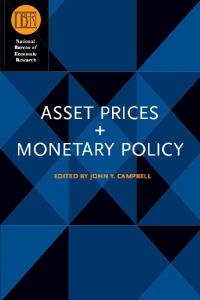
Figure 1.1. The terms of trade and the real exchange rate. unchanged; or it might fail because of changes in the real exchange rate, the terms of trade remaining constant. There is no reason, in theory, to expect any systematic relation between changes in the terms of trade and changes in the real exchange rate. The money prices of three variables - prices of domestic goods, exports, and imports - cannot, in general, be collapsed into two monetary variables, the prices of domestic and prices of international goods. Nor can two real variables - the terms of trade and the real exchange rate - be collapsed into a single variable called the real exchange rate. The terms of trade can worsen (improve) because of increases (decreases) in the price of imports or decreases (increases) in the price of exports: In the first case the real exchange rate appreciates; in the second, it depreciates. Thus, in Figure 1.1, the real exchange rate corresponds to the RER curve (given the price of domestic goods), whereas the terms of trade is given by the slope of the TOT line. The terms of trade are determined by external factors while the real exchange rate, by internal factors. An externally induced fall in the terms of trade shifts the TOT line to, say, TOT'. At fixed exchange rates, the equilibrium would move to R if the fall in the terms of trade were due to a rise in import prices, and to T if it were due to a fall in export prices. With given prices of domestic goods, the real exchange rate would therefore depreciate in the former and appreciate in the latter case.
Stabilization policies in semi-open economies
23
Under flexible exchange rates and a fixed money supply, the nominal exchange rate would appreciate when faced with an increase in the price of imports, and depreciate when faced with a decrease in the price of exports, in both cases leading to an equilibrium between T and R, such as that at U, where the real exchange rate is unchanged.3 Other external factors The Chilean stabilization plan offers an example where the breakdown of the stabilization plan coincided with a fall in the terms of trade. The rise in the price of oil in 1979 was followed by the collapse of copper prices in 1982 (from $1.00 per pound in 1980 to $0.67 in 1982). The first change depreciated, and the second appreciated the real exchange rate; but both worsened Chile's terms of trade.4 Changes in the terms of trade are not the only external factors affecting success of failure of stabilization plans. Changes in the nominal exchange rate and the interest rate affected many of the developing countries (including Chile) in the early 1980s. The dollar appreciated strongly with the shift in the U.S. policy mix under President Ronald Reagan. Fiscal expansion and monetary tightness led to appreciation of the dollar and soaring real interest rates, with a short but sharp recession in 1982. The appreciation of the dollar helped to overvalue the peso, high real interest rates aggravated the burden of debt service, and the world recession weakened the market for nontraditional exports. Several other countries' attempts at stabilization have failed partly because of external factors. Argentina's and Uruguay's stabilization plans in the late 1970s and early 1980s provide another example. In 1979, the U.S. government imposed an embargo on grain exports to the Soviet Union, in reaction against its invasion of Afghanistan. The Soviet Union turned to Argentina as an alternative source, and the resulting export boom made it possible to introduce Argentina's stabilization plan. Huge spillover effects of the boom were experienced in the form of a massive capital influx to neighboring Uruguay, largely directed at building the resort center of Punte del Este; this was the "Afghanistan effect." When the boom subsided in 1981 and 1982, budgets became unbalanced and the stabilization plans of both countries collapsed. The plans were all undermined by 3
4
The change in the real exchange rate depends on the weights attached to imports and exports in the index of international goods prices. Given a fixed money supply and flexible exchange rates, the real exchange rate would be unchanged when the terms of trade change if the weights in the prices of international goods in the real exchange rate index were the same as the weights of those goods in the demand for money function. See Edwards (1984, 1985); Corbo (1985, 1986); Edwards and Cox-Edwards (1987); and Cuadra and Valdes (1992) for analyses of the Chilean case.
24
Robert Mundell
the combination of a rising dollar, falling terms of trade, high real interest rates, and the world slump. In the cases of both Argentina and Uruguay, however, fault also lay in the inability of the authorities to maintain fiscal solvency. External factors sometimes combine with policy mistakes to leave a country saddled with an overvalued real exchange rate. The North American Free Trade Area Agreement had been signed by President Ronald Reagan of the United States and Prime Minister Brian Mulroney of Canada on January 2, 1988. A year earlier, the Bank of Canada had dedicated monetary policy to the achievement of a zero inflation rate, raising interest rates several percentage points above those in the United States. Both policies led to a massive influx of capital that pushed up the Canadian dollar by 30 percent. The current account, which had been in approximate balance in the first half of the 1980s, went into a deficit of over 4 percent of GDP. By 1992 the restrictive monetary policy was relaxed, but only after the economy had moved into severe depression, with unemployment, above 10 percent, higher than in any other G-7 countries with the exception of the United Kingdom. The policy mistake was in relying on an appreciating exchange rate as the main vehicle for enforcing (without success) price stability. An analogous situation arose in the United Kingdom. The announcement of completion of the common market in the Economic Community led to a massive influx of capital into London and a real estate boom. The pound, which had been as low as U.S.S1.05 in 1985, soared, going above U.S.S1.90 when the United Kingdom made the fateful decision to enter the exchange rate mechanism (ERM) of the European Monetary System (EMS), at the high rate of DM 3 per pound. The capital inflow, combined with the overvalued pound, led to soaring imports and sluggish exports, and led to the largest recession in postwar history, with unemployment exceeding 10 percent. When the German unification shock struck the EMS, the United Kingdom opted out, allowing the pound to depreciate against both the dollar and the mark. The policy mistake was not so much in entering the ERM of the EMS, but in entering it at a greatly overvalued rate, temporarily pushed up by an influx of capital.
The problem of capital imports
Stabilization failures cannot be understood without consideration of the role played by capital movements. But the benign or harmful effect of capital movements in stabilization and liberalization plans has been a subject of considerable dispute. One of the most controversial questions has
Stabilization policies in semi-open economies
25
been whether liberalization of trade should be accompanied by liberalization of the capital account, or whether the latter should be delayed. The literature seems to be against simultaneous liberalization of the capital account. Among the famous cases where capital imports have allegedly upset stabilization plans, one must include Korea in 1966-70, and Chile, Argentina, and Uruguay in 1978-82. The situation of Chile came as close to a controlled experiment as is likely to exist in economics. The combined liberalization and stabilization programs seemed to be upset by the capital imports that inundated Chile in 1978-82. That country's fiscal deficit had reached 25 percent of GDP in 1973, but it was brought under control by 1977 and 1978, making financial stabilization for the first time feasible. At the same time Chile moved toward free trade: Nontariff barriers were first converted to tariff equivalents, and then the tariff rates were systematically lowered. From an average of 94 percent in 1973, average tariff rates fell to 44 percent at the end of 1975, 33 percent at the end of 1976, 18 percent at the end of 1977, 12 percent at the end of 1988, and 10 percent after 1979. Exchange rate stabilization proceeded in steps: First, multiple exchange rates were unified into a single rate; second, beginning in February 1978, the tablita - a depreciating crawl of the peso at preannounced rates - was introduced, which held depreciation to 24 percent in 1978, an additional 14 percent depreciation in 1979 until, in the middle of that year, the peso was fixed at 39 pesos to the dollar and held at that rate until the collapse of 1982. The inflation rate, which had been 92 percent in 1977, came down to 35 percent in 1980, 20 percent in 1981, and 10 percent in 1982. Real GDP rose at a rate of 9.9 percent in 1977, 8.2 percent in 1978, 8.3 percent in 1979, 7.8 percent in 1980, and 5.5 percent in 1981 (only to fall by 14.1 percent in 1982). The spectacular success of the Chilean stabilization policy was more apparent than real, more transitory than permanent. The deceleration and then fixing of the exchange rate was achieved only at high real interest rates, which, in conjunction with the rise in the marginal efficiency of capital due to trade liberalization, led to massive inflows of capital from abroad. Short-term capital inflows more than doubled to $0.6 billion in 1977, tripled to $1.8 billion in 1978, $1.9 billion in 1979, $3 billion in 1980, and $4.3 billion in 1981. The latter figure for 1981 was larger than Chilean exports of $3.6 billion in that year. These capital imports financed an explosion of imports and a contraction of exports: From imports of $2.9 billion in 1978, imports rose to $3.6 billion in 1982. The current account deficit soared from $0.5 billion in 1977 to $4.7 billion in 1981, equal to 14.5 percent of GDP. What are the lessons from the Chilean episode? One, already noted,
26
Robert Mundell
is that the use of the exchange rate policy as a deflationary device was incompatible with independently rising wage rates; it would have been better to put wages under the tablita along with the exchange rate, as a temporary device during the transition period. Even so, the excessive growth of real wages would have been checked by rising unemployment had it not been for excessive capital imports, drawn in by high real interest rates. In effect Chile's borrowing sustained real wages and living standards beyond its means over the stabilization period. In theory, capital imports should be a help rather than a hindrance; the essence of capital imports is that they allow a country to achieve economic targets earlier than would otherwise be possible. Unfortunately, however, there are some negative externalities. One is that the borrowing goes into consumption rather than investment, permitting the capital-importing country to live beyond its means, pay higher real wages, or finance a budget deficit, without any offset in future output with which to service the loans. Even if the liabilities are entirely in private hands, the government may feel compelled to transform the unrepayable debt into sovereign debt rather than allow execution of mortgages and other collateral. Argentina, in 1990-92, represents another case where stabilization policy has fallen victim to overvaluation of labor paid for by capital imports. To build up confidence in the exchange rate, Argentina enacted a convertibility law that allowed Argentines to use dollars in local transactions, required the central bank to hold a dollar in reserve for every peso in circulation, and forbade the central bank from financing budget deficits; in effect Argentina went on a "currency-board" system. This policy was successful in reducing inflation rates from 800 percent in 1990 to 56 percent in 1991 and to less than 20 percent in the first part of 1992. But it was still too high to keep the Argentine economy competitive at fixed exchange rates; wage rates continued to rise faster than productivity. The trade balance, which had grown to $8.6 billion in 1990, fell to $4.7 billion in 1991 and is expected to be -$1.0 billion in 1992, the first deficit in more than a decade. The current account, which was in surplus by $1.9 billion in 1990, was $2.7 billion in deficit in 1991, and is expected to be much worse in 1992. To counter these alarming trends, the minister of finance, Domingo F. Cavallo, announced, on October 28, 1992, tax and subsidy measures to stimulate exports, partly reversing the free-market deregulation plan he had introduced in March 1990. By November 1992, there has been a flight from the peso and interest rates on short-term peso loans were up to more than 50 percent. These examples raise questions about the usefulness of increased capital imports as part of a stabilization program. Capital imports are neither good nor bad in themselves: They finance an excess of domestic spending
Stabilization policies in semi-open economies
27
over income and, in principle, allow a country to achieve economic objectives sooner than would otherwise be possible; on the other hand, they also increase a country's net external debt. Unless capital imports increase productive capacity by enough to yield a net rate of return higher than debt service, countries do not gain in the long run by capital imports. There are two risks to capital imports. First, it may undermine a monetary stabilization policy; second, it may serve to finance wage increases and therefore consumption spending in the labor sector above the marginal productivity of labor; this is a recipe for bankruptcy. Even if the borrowing is entirely incurred by the private sector, it can build up problems for the country as a whole in the future: In the debt crisis of the 1980s, several governments found it necessary to transform private debt into sovereign debt, nationalizing companies and banks rather than acquiescing in their bankruptcy. Korea's successful stabilization Korea, in 1964, introduced trade reforms and monetary stabilization coupled with a substantial devaluation of the won, from 130 to 255, and then (in 1965) to 271 against the dollar. Inflation was brought down to about 10 percent; interest rates were raised to positive real levels; a fiscal reform led to a doubling of tax revenues; and exports and investment grew rapidly. These measures, in conjunction with the trade liberalization, had raised the marginal efficiency of capital and led to substantial short-term capital imports, threatening to appreciate the exchange rate. The authorities had three alternatives: (1) to let the exchange rate appreciate; (2) hold the exchange rate and allow a corresponding monetary expansion; and (3) control capital imports. The first alternative would have immediately reduced the competitiveness of Korea's new industries in export market; the second would have brought on a return to inflation; and the third would have been inconsistent with the liberalization plan. The second option was chosen, the influx of foreign exchange reserves was monetized, domestic spending increased, and the current account deficit soared. Inflation returned but overvaluation was prevented by a slow depreciation of the currency. Successful stabilization in Korea had to await the 1980s. The Korean stabilization policy of 1981-89 stands out as an example of successful stabilization policy. It was successful on several grounds. Prior to 1982, Korean inflation had typically hovered around 20 percent; but from 1982-89, it was always less than 7 percent. Throughout this period GDP at constant prices achieved the remarkable average growth rate
28
Robert Mundell
of 9.7 percent, the most remarkable performance of any economy in the 1980s.5 What was responsible for the Korean success in contrast to the failure of so many other stabilization plans? One answer is that Korea avoided the mistakes of using the exchange rate as the active instrument for disinflation and thus avoided overvaluation. Over the early period, from 1981 to 1984, the exchange rate was managed by a downward crawl at a rate of depreciation that slightly exceeded the inflation rate.6 At the same time interest rates were cut to anticipate the declining inflation rate. The policy of exchange depreciation was especially important in these years, 1981-85, when the dollar was the strongest currency in the world. In the following years, from 1985-89, three additional external factors contributed to the Korean success. First, the price of oil fell drastically, improving Korea's terms of trade and raising the marginal productivity of capital in Korea. Second, interest rates declined from their peak and lowered Korea's debt-service problem. Third, the dollar declined, allowing Korea to maintain its competitiveness despite some pressure from the United States for appreciation. Korea's success was therefore due to sound policy management in combination with fortuitous external circumstances. Policy gets the credit for the early years of success; and external circumstances for the last half of the decade. In the first phase, Korea not only balanced its budget and applied monetary restraint, but it also was able to lower nominal interest rates pari passu with the reduction in the inflation rate; meanwhile the won was allowed to depreciate to prevent overvaluation. The continuation of the growth boom was definitely helped by changes favorable to Korea in the world environment. Recent developments in Korea
Since 1981 the Korean economy has been in what appears to be a perpetual boom, with a high and even rising share of investment in GDP that reached 39 percent in 1991. From 1982 through 1989, this performance was accompanied by price stability in the sense of an inflation rate averaging 5 percent and a currency that appreciated slightly against the dollar, from an average of 731 per dollar in 1982 to 671.5 per dollar in 1989. Over this period, the budget was in essential balance and the current account balance continually improved, moving into a surplus, equal to 4.4 percent of GDP in 1986. The current account surplus rose to 7.5 percent of GDP 5
6
After a dip to 6.2 percent in 1989, the real GDP growth rate recovered to 9.2 and 8.4 in 1990 and 1991. See McKinnon (1991: 78) for a discussion of this point.
Stabilization policies in semi-open economies
29
in 1987, and 8.1 percent of GDP in 1988 (equal to $14.2 billion), but falling to 2.4 percent of GDP in 1989. From 1989, however, two worrisome features appeared in the Korean economy. One was an increase in the rate of inflation to 10.7 percent in 1990 and 10.8 percent in 1991, falling slightly, however, in 1992. The other was the turnaround in the current account. The surpluses in the four years 1986 to 1989 - thought by some to be "structural" - turned into deficits of 0.9 percent of GDP in 1990 and 3.1 percent in 1991; it is expected to be in deficit also in 1992 and 1993. An even larger turnaround occurred in the trade balance: From $11.5 billion in 1988, it fell to $4.6 billion in 1989, to a deficit of $2.0 billion in 1990, and a deficit of $7.0 billion in 1991. In the period 1989 through 1991, the fall in exports to the United States and Japan was more than made up by the rise in exports to the rest of the world, so that Korea has managed to increase its global exports in those years; imports from the United States, Japan, and the rest of the world, however, rose much more rapidly than exports. Due to the current account deficit, Korea's net external debt has been rising. Gross external debt rose from $33.1 billion in 1989 to $38.5 billion in 1991, and is expected to rise to $52.8 billion at the end of 1992. On the other hand, Korea's overseas assets totaled $27.5 billion in March 1992 so that net external debt was only $ 13.5 billion (but expected to rise substantially by the end of the year). In 1991, according to the balance-of-payments accounts, Korea received income from investments overseas of $3.4 billion and paid out $3.8 billion on foreign investments in Korea (according to the national accounts, net factor payments abroad were $1.5 billion). A missing component of the analysis relates to the demographic factor. The position of a country's current account is influenced by its rates of net saving and investment, both of which are affected by changes in the age distribution of the population.7 What is often called "structural" balances are in fact endogenous to the population structure. Tighter money, high interest rates, and a falling stock market greeted the liberalization of the capital market in January 1992. The stock market rallied with the liberalization, but then continued its downward track, the Korean Composite Stock Price Index (KOSPI) falling below 560 in June 1992, from its peak of 918.6 in 1989. Current policy
Current economic policy is directed at containing inflation and reducing the exploding current account deficit. To this end the current plan aims to 7
See Mundell (1990, 1992a) for analysis of how demographics affects the balance of payments; and Kim (1992) for a recent examination of stages in the balance of payments in several countries with some focus on Korea.
30
Robert Mundell
keep wage increases to 5 percent, has put curbs on imported goods, and encouraged the substitution of domestic-made machinery. The Bank of Korea is trying to maintain a restrictive monetary policy in order to cool down the country's overheated economy and to stabilize prices, keeping the growth of the broad measure of the money supply (M2) within 18.5 percent, necessary to achieve the target inflation rate below 9 percent (with real GDP growth of 7 percent). The two main problems with the economy relate to the persistence of moderate inflation and the deterioration of the current account. In both these respects the performance of the economy has been worse than that achieved in the 1980s. A major source of the difficulty is the influx of foreign capital that simultaneously undermines monetary stability and finances the excess of expenditure over income that constitutes the current account deficit. The dilemma is that, on the one hand, more restrictive monetary policies are needed to bring down the inflation rate; but, on the other hand, tight money will attract more capital and worsen the current account. In principle, an open capital market is likely to be conducive to economic efficiency. Yet capital imports have negative side effects, as most of the heavily indebted countries now realize. The private sector has a tendency to incur debt that is often later turned into sovereign debt, as an alternative to bankruptcy. Real GDP in Korea has been growing more rapidly than nearly every other country, fed by investment ratios near 40 percent of GDP. With wage rates, of a skilled labor force of 19 million, in the range of only $4.50 an hour, the return to capital remains extremely high. It may be better for Korea to rely less on capital imports even if it would mean reducing the share of investment in GDP to 35 percent. A small reduction in the rate of growth of GDP might not involve much of a reduction in growth of GNP, if debt service is taken into account. In the late 1980s, Korea seemed to have arrived at a new "stage" in its balance of payments, with cumulative current account surpluses amounting to $33.7 billion in 1986-89; this surplus enabled Korea to reduce its net debt to $13.5 billion, and its net debt service to about $1 billion. Already in 1986 Korea had become a "mature-debtor-lender" with an export surplus, and was fast approaching a position where it was no longer a creditor. But the turnaround in policy in 1989-92 has put the shift to creditor status a long way off. Was Korea's strong external position in 1986-89 merely a lucky confluence of the three favorable external circumstances - low dollar, low interest rates, and low price of oil? The answer is no; the "three lows" are even lower today! The only unfavorable external factor for Korea was the U.S. slump and the emergence of a growth slump in Japan. But this was
Stabilization policies in semi-open economies
31
more than made up by the favorable situation in Europe. The unification of Germany brought about a reversal of the German trade balance; and Korea was able to increase its exports to Europe. At the same time the prospects for expanding trade with China appear better than ever before. On balance, then, the external situation has been favorable to Korea and will probably be increasingly favorable with the progress of the global recovery. The demographic factor should also be taken into account in assessing the stages of Korea's balance of payments. Age distribution affects the balance of payments because different generations have different balances of investment and saving. Dependents - both young and old - are net consumers; whereas the working age population are net producers. But the ratio of dependents to workers - the "dependency ratio" - is only part of the demographic story and not the most important part. More important is the difference between the investment and saving patterns of workers of different generations. While both "junior" and "senior" workers save substantially, junior workers invest more (on houses, consumer durables, etc.) than they save and are thus net borrowers; whereas senior workers save more than they invest and are thus net lenders. Demographic shocks (e.g., a baby dearth or boom) create population bulges in one group or the other that introduce a cyclical pattern to domestic spending relative to income - and therefore the current account - that reverberates over the generations. It would be a mistake to evaluate Korea's prospects for generating future current account surplus without an examination of the two key demographic variables: the dependency ratio and the juniorsenior work ratio. "How does Korea fit into the demographic cycle?" is a question crying out for an answer. Various conditions have to be met for Korea to turn its current account around; they relate to the goods and services market, the capital market, and the money market.8 One way for Korea to turn its current account around is to move toward increased net capital exports, partly by encouraging Korean direct capital exports, partly by withholding taxes on unwelcome short-term capital imports, and partly by the development of a larger foreign exchange reserve invested in interest-bearing dollar assets. This would almost certainly require also a fall in the real exchange rate, which, in practice, could only be accomplished by a fall in the nominal exchange rate, an increase in the number of won per dollar. Currency depreciation always carries the risk of an increase in the rate 8
To improve the current account, it is simultaneously necessary to increase (1) the gap between GNP and domestic expenditure; (2) the capital and/or reserve account; (3) the sum of the domestic excess demands for securities and money; and (4) the rest-of-the-world counterparts for these categories. For a discussion of the sixteen macroeconomic relation-
32
Robert Mundell
of inflation. With respect to exchange rate policy, it is always desirable to steer a balanced course between the Scylla of overvaluation and uncompetitiveness and the Charybdis of undervaluation and inflationary pressure. The Korean won appreciated significantly against the dollar from an average of 870 in 1985 to 671 in 1989; since 1989, it has depreciated. The current won is about 15 percent higher against the dollar than it was in 1985 despite the fact that prices have risen more rapidly than in the United States and wages have soared. A lower won would almost certainly be a necessary concomitant of renewed net capital exports and a turnaround in the current account.9 References Brock, Philip L. (ed.). (1992). If Texas Were Chile: A Primer on Banking Reform. San Francisco: ICS Press. Brock, Philip L., Michael B. Connolly, and Claudio Gonzalez-Vega (eds.). (1989). Latin American Debt and Adjustment: External Shocks and Macroeconomic Policies. New York: Greenwood Press. Corbo, Vittorio. (1985). Reforms with Macroeconomic Adjustment in Chile during 1974-84. World Development 13: 893-916. (1986). The Role of the Real Exchange Rate in Macroeconomic Adjustment: The Case of Chile, 1973-82. Paper presented at the Central Bank of Ecuador Conference on Trade Liberalization, Quito, January 1992. Corbo, Vittorio, and Jaime de Melo (eds.). (1985). Liberalization with Stabilization in the Southern Cone of Latin America. World Development 13: 863-66. Cuadra, Sergio de la, and Salvador Valdes. (1992). Myths and Facts about Financial Liberalization in Chile. In Brock (1992): 11-101. Dornbusch, Rudiger. (1992). Disinflation and Real Exchange Rates. Mimeograph copy of paper presented at the University of Chicago International Economics Workshop Conference, October 24. Dornbusch, Rudiger, and Yung Chul Park. (1987). Korean Growth Policy. Brookings Papers on Economic Activity 2: 389-444. Edwards, Sebastian. (1984). The Order of Liberalization of the External Sector in Developing Countries. Princeton Essays on International Finance, no. 156, Princeton University. (1985). Stabilization and Liberalization: An Evaluation of Ten Years of Chile's Experiment with Free Market Policies, 1973-84. Economic Development and Cultural Change 33 (January): 223-54. Edwards, Sebastian, and Alejandra Cox-Edwards. (1987). Monetarism and Liberalization: The Chilean Experiment. Cambridge, Mass.: Ballinger. Kim, Sang Kyom. (1992). The New Approaches to Stages in Analysis of the Balance of Payments. Ph.D. diss., University of Pennsylvania.
9
ships that must be changed when the current account is altered, see Mundell (1989a, 1989b, 1991a). To the extent that Korea is free to do so, the authorities should allow the won to depreciate against the dollar and perhaps also the yen and the mark even if those currencies depreciate against the dollar.
Stabilization policies in semi-open economies
33
Lizondo, S., and P. Montiel. (1989). Contractionary Devaluation in Developing countries. IMF Staff Papers 36 (March): 182-227. McKinnon, Ronald I. (1991). The Order of Economic Liberalization: Financial Control in the Transition to a Market Economy. Baltimore: Johns Hopkins University Press. Montiel, P., and J. Ostry. (1991). Macroeconomic Implications of Real Exchange Rate Targeting in Developing Countries. IMF Staff Papers 38 (December): 872-900. Mundell, Robert A. (1989a). Trade Balance Patterns as Global General Equilibrium: The Seventeenth Approach to the Balance of Payments. Rivista di Politica Economica 79, no. 10 (September): 9-60. (1989b). The Global Adjustment System. Rivista di Politica Economica 79, no. 12 (December): 351-464. (1989c). Latin American Debt and the Transfer Problem: Introduction. In Brock, Connolly, and Gonzalez-Vega (1989): 1-17. (1990). The International Distribution of Saving: Past, Present and Future. Rivista di Politica Economica 80, no. 10 (September): 5-56. (1991a). The Great Exchange Rate Controversy: Trade Balances and the International Monetary System. In Fred Bergsten (ed.), International Adjustment and Financing: The Lessons of 1985-1991. Washington, D.C.: Institute for International Economics, 187-239. (1991b). The Overvalued Canadian Dollar. In Fakhari Siddiqui (ed.), The Economic Impact and Implications of the Canada-U.S. Free Trade Agreement. Lewiston: Edwin Mellon Press, 75-112. (1992a). Fiscal Policy and the Theory of International Trade. In Herbert Giersch (ed.), Money, Trade and Competition: Essays in Memory ofEgon Sohmen. Berlin: Springer-Verlag, 145-63. (1992b). Stabilization Policies in Less Developed and Socialist Countries. In Emil-Maria Claassen (ed.), Stabilization Policies in Less Developed and Socialist Countries. San Francisco: International Center for Economic Growth, 122-38. (1992c). The Quantity Theory of Money in an Open Economy: Variations on the Hume-Polak Model. In Jacob Frenkel and Morris Goldstein (eds.), International Financial Policy: Essays in Honor of Jacques J. Polak. Washington, D.C.: International Monetary Fund, 167-74.
CHAPTER 2
Monetary regime choice for a semi-open country Jeffrey A. Frankel
It is natural that a country that industrializes will also begin to liberalize its goods and financial markets. As it seeks to move more fully into the international community of industrialized countries, it will be called upon to allow ever more aspects of its economy to be determined in the marketplace rather than by the government. But it does not follow that every aspect, every macroeconomic variable, should be determined by the marketplace. To focus on a clear example, the exchange rate should not necessarily be determined in the marketplace. Letting the exchange rate float makes more sense if the monetary authorities have decided to fix the money supply (or other nominal quantity). But an equally admissible alternative plan is to fix the exchange rate and let the money supply do the adjusting. One must choose among equally plausible regimes. To make this point is not to knock down a "straw man." The U.S. Treasury has in recent years advised newly industrialized countries (NICs) in East Asia that free-market principles necessarily imply free-floating exchange rates.1 Free-marketeers Milton Friedman and Beryl Sprinkel might agree with that choice, but free-marketeers Robert Mundell and Jack Kemp would not. 1
Democracy, discipline and deficits
This chapter reviews choices among regimes facing a relatively small, trade-oriented, liberalizing, industrializing country. We begin by observing that the problem is neither interesting nor realistic unless due allowance is 1
In October 1988 the U.S. Treasury, in its "Report to the Congress on International Economic and Exchange Rate Policy" required by the Omnibus Trade and Competitiveness Act of 1988, concluded that Korea and Taiwan "manipulated" their exchange rates, within the meaning of the legislation. Financial policy talks with Korea followed, in February and November 1990.1 discuss recent liberalization of Korean financial markets and foreign exchange markets, and the role of U.S. pressure, in Frankel (1993b). 35
36
Jeffrey A. Frankel
made for market failures, such as sticky prices, as well as political failures, such as populist spending binges. On the one hand, if there are no sticky prices, frictions, or other market failures, then it follows that everything should indeed be left up to the market.2 If there are no issues of political economy, on the other hand, then the government should retain complete discretion, so as to be free in the future to move all levers in optimal response to the latest developments. Issues of political economy are particularly relevant if a country is undergoing a transition to democracy at the same time as its economic transition. It is not that an authoritarian government is more likely to produce good economic policies than a democracy.3 Authoritarians frequently meet neither of the two criteria one wants from a philosopher king: being well informed and being well intentioned. But democracies are routinely subject to certain pressures in their economic policy making. Awareness that this is so must heavily condition the problem of what regime to choose in advance.4 Indeed the argument for the government precommitting to any regime, rather than retaining short-term discretion, rests on the existence of these pressures and the need for discipline to resist them. To be more specific, there are good political economy reasons for making (1) a precommitment not to inflate, and (2) a precommitment not to overborrow. The first problem, a bias toward excessive monetary expansion, was amply demonstrated in the worldwide inflation of the 1970s. It gave rise to a burgeoning literature on the desirability of time-consistent rules for monetary policy, that is, credible precommitments to a nominal anchor. It also gave rise to a declaration by major central banks of an allegiance to monetarism. But the 1980s left many central bankers disillusioned with monetarism, and the question of the optimal nominal anchor is still an open one. The second problem, overborrowing, was amply demonstrated in the international debt crisis of 1982. In theory, openness to international capital flows offers enormous advantages: the ability to borrow abroad to finance development of a country where the rate of return to investment at home is high, the ability to smooth spending out over recessions and other short-term fluctuations in income, and the ability to diversify risk internationally. In practice, the option to borrow or lend internationally is misused as often as it is used in the optimal way that our theories assume. 2
3
4
The authorities still have to choose a money supply. But in a sufficiently perfect world, the choice makes no difference. Economists have begun to tackle issues like these that they used to leave to political scientists. Barro (1989), e.g., finds in a cross-section of countries that a measure of the extent of political rights is positively correlated with growth. On populism, see Dornbusch and Edwards (1991).
Monetary choice for a semi-open country
37
One has only to observe that countries tend to borrow internationally when they are undergoing temporary booms, and to pay back in downturns, to realize that the theories of intertemporal optimization are missing something. The explanation for such procyclical borrowing probably lies in the nature of the supply of funds from imperfectly informed lenders and in the political economy of the local groups who get to spend the money.5 Other possible sources of imperfection in international capital markets include flows motivated by tax evasion, speculative bubbles, contagion, and the lack of an international enforcement mechanism in the event of default. The point is that a case could be made for keeping controls on capital inflows, in order to avoid the temptation to overborrow. The argument for precommitting not to inflate and the argument for precommitting not to borrow abroad could be seen as two components of a more general precommitment not to run an excessive government budget deficit. Such deficits can be financed either by monetization/inflation or by foreign borrowing. In a country with sufficiently developed domestic financial markets, they can also be financed by borrowing from domestic residents. The United States sought a fiscal commitment mechanism in the Gramm-Rudman-Hollings legislation. The members of the European Community sought a fiscal commitment mechanism in the terms of the Maastricht Treaty. Both experiments have to date been unsuccessful. Taking our cue from the G-7 countries, we will assume in the remainder of this chapter that precommitments against domestic borrowing and international borrowing are not practical, presumably because the advantages of being able to run deficits at times are too great. We take as given that the country in question is opening up its capital markets. There do exist, after all, a few countries like Korea that have tended to exhibit the self-control necessary to avoid overborrowing. (Korea in the 1970s mostly used its international borrowing for high-return investment rather than private or government consumption, and in the 1980s did not wait for international bankers to cut off lending before taking the measures to adjust to higher world borrowing costs.) Korea appears, in any case, to have embarked on a path of financial liberalization. We henceforth focus, rather, on the choice of exchange rate and monetary regimes, taking financial liberalization as given. 2
The choice of fixed versus flexible exchange rate
The debate between adherents of fixed or flexible exchange rates is often phrased as a choice between absolutes. But the optimal currency area literature introduced thirty years ago by Mundell (1961) and McKinnon 5
E.g., for the case of commodity-producing countries, Cardenas (1991).
38
Jeffrey A. Frankel
(1963) demonstrated clearly that one choice cannot be right for all countries. It does not seem sensible for an extremely small open country or province to have an independent currency. This point has been illustrated anew in recent years by plans for European Monetary Union, although Europe has also demonstrated (in the 1992 crisis) the practical difficulty of knowing when a country is in fact sufficiently open to give up its monetary independence. We will review the advantages of flexible exchange rates, and then the advantages of fixed exchange rates. We will take special note of the aspects of a particular country that determine which set of advantages is likely to dominate. 2.1
The advantages of flexible exchange rates
The advantage of flexible rates is that, freed of the obligation to keep the exchange rate fixed, monetary policy can respond independently to disturbances. When a country opens up its financial markets to international capital flows, the point becomes stronger. Monetary policy becomes a powerful instrument. A monetary expansion under floating exchange rates has much of its effect via the international channel - a depreciation of the currency and the resulting stimulus to net foreign demand - supplementing the traditional channel of a lower real interest rate and resulting stimulus to domestic demand. The Mundell-Fleming model originally showed that the more highly mobile is capital, the stronger this effect is. In the limit of perfect capital mobility, the expected rate of return in the domestic country is tied to the world rate of return. If exchange rates are fixed, there is no scope for monetary policy to have independent effects at all. In that case, a flexible exchange rate is a sine qua non of monetary independence. How important is it to have an independent monetary policy, and thus by implication to have a flexible exchange rate? This depends on two questions. (1) How often does the domestic country experience a disturbance that calls for a response that differs from what is occurring among its neighbors? (2) If an independent monetary response (a reduction in interest rates or a devaluation) is not an option, what alternative means of adjustment are there? The first question in turn subdivides into two questions, (la) To what extent does the domestic country experience shocks that are different from those experienced by its neighbors? Here the extent to which the economies are integrated by trade is key6 (lb) When the domestic country expe6
Some economists assume that an increase in trade between neighbors reduces the correlation between their shocks, because it increases specialization, and thus ironically makes the Optimum Currency Area less likely to hold (e.g., recently, Bayoumi and Eichengreen
Monetary choice for a semi-open country
39
riences a shock similar to that of its neighbors, to what extent does it wish to respond independently, for example, because of a different priority placed on fighting inflation relative to sustaining output and employment? This is largely a matter of the extent to which the countries have divergent values. If the answer to these questions is "not to a great extent," then the region should be happy to share the monetary policy of its neighbor. But otherwise, it will often find itself, in the aftermath of a shock, wishing to make some sort of independent response or adjustment. The second question concerns alternative means of adjustment, which, if available, might make a deliberate monetary response unnecessary. This question also has two components. (2a) If a region experiences a negative shock, such as a loss in demand for its products, and there is no effective macroeconomic response, can its workers easily move to other regions? Labor mobility across geographic boundaries is the optimum currency area criterion on which the original Mundell (1961) article focused. It depends both on formal barriers to travel and migration, such as those recently relaxed within Europe, and more broadly on linguistic and cultural compatibility. Recent research has shown that when a region of the United States experiences a negative shock, the major means by which markets eventually adjust is not a gradual reduction in wages, but a gradual movement by workers to other regions of the United States.7 (2b) If all other means of adjustment fail (macroeconomic expansion, devaluation, lower wages, and out-migration), is there a supraregional or supranational federal system that will undertake fiscal transfers to the depressed region or country? A federal fiscal system operates in the United States,8 and France fiscally supports the franc-pegging governments of West Africa. But recent developments in Europe suggest that there is not as much political will in the northern countries to make transfers to other countries as advocates of European Monetary Union had hoped. The foregoing cataloging of the various factors that might make an independent monetary policy unimportant or unnecessary shows a common theme. When a region is highly integrated with its neighbors - sharing common disturbances and values, or with easy movement of labor or transfers across its borders - monetary independence is less necessary. We must now ask what advantage there might be in giving up monetary
7 8
[1992] and Blanchard and Muet [1993]). This would be an excellent subject for future research; the question must depend on the reason for the increased trade, and the nature of subsequent shocks. I believe, however, that for most sources of trade and most shocks, an increase in trade tends to increase the correlation of shocks, and thereby to strengthen the argument for pegging to neighbors. Blanchard and Katz (1992). Sachs and Sala-i-Martin (1989) document the transfers from the U.S. federal government that flow automatically to a U.S. state experiencing a downturn.
40
Jeffrey A. Frankel
independence. Even if the usefulness of monetary expansion and devaluation diminishes when there are alternatives, are these not options that are always of some use to retain? We have only considered the advantages of flexible exchange rates. We must now consider the advantages of fixed exchange rates. 22
The advantages of fixed exchange rates
The advantages of a fixed exchange rate, again, fall into two broad categories. (1) First, stabilizing the currency reduces exchange rate uncertainty facing exporters and importers, as well as international borrowers and lenders. The discouraging effect on international trade and finance that exchange rate risk might have was one of the most important arguments used by those who opposed a general move to floating exchange rates before 1973. (2) Second, a fixed exchange rate can serve as an effective nominal anchor for monetary policy, and thus can assure price stability. We consider each advantage in turn. The hypothesized advantages of exchange rate stability per se constitute too large a subject even for the sort of capsule summary we are pursuing here. Critics of the way floating rates have operated among the G-7 countries over the past twenty years have tended to focus more on longer-term "misalignments" rather than short-term volatility. Misalignments such as the 1984-85 overvaluation of the U.S. dollar are perceived to impose longterm costs in the form of protectionist barriers and a diminished capital stock in tradable goods sectors. Key to evaluating arguments regarding either long-term misalignments or short-term volatility is a means of evaluating whether private financial markets, with their occasional speculative bubbles and other possible defects, are more or less likely to produce unneeded or undesirable exchange rate movements or misalignments than is the political process, with all its defects, under a pegged-rate system. This debate is very much unsettled. 2.3
The effect of exchange rate variability on trade
The danger of misalignments is not the major motivation behind European efforts to stabilize exchange rates among themselves. Promoting intra-European trade has been a more important motivation. Economists reviewing the post-1973 record have tended to be skeptical about the effect of exchange rate uncertainty on trade. They point out that markets in forward exchange and other derivatives allow an importer, say, to hedge the risk of an increase in the price of foreign currency. It would be a mistake, however, to think that all exchange rate risk can be hedged
Monetary choice for a semi-open country
41
in this way, even in theory. Although any given importer can hedge his exposure, someone, somewhere, will have to bear some exchange risk, and that person will demand a price to compensate him for doing so. The empirical record on the effect of exchange rate variability on trade since 1973 is mixed. Notwithstanding the high level of volatility in the twenty years since exchange rates began to float, the international volume of trade has grown rather rapidly. Time series studies such as Hooper and Kohlhagen (1978) found only very limited evidence of effects. Some later studies found relatively more effects, but overall surveys of the subject do not present a strong case for an effect on trade. The problem with the time series studies is that other factors have changed since 1973, at the same time as exchange rate variability. (Some factors leading to greater trade over the past twenty years are economic growth, reduced tariff barriers, and possibly lower costs of transportation and communication.) If a quantum change in the level of uncertainty would have to be sustained for a number of years before it could be reliably perceived, let alone before it could lead to a reallocation of resources between traded goods and nontraded goods, twenty years of time series data are perhaps not the most promising place to look. Together with Shang-jin Wei, I have applied to this problem a crosssection data set of bilateral trade flows between 1,953 pairs of countries. We use the gravity model, to explain the volume of bilateral trade (in logarithmic form) by four basic determinants: the sizes of the two countries, their GNP/capitas, the distance between them, and a dummy variable indicating whether they share a common border. In Frankel (1992, 1993), we see how much of the residual can be explained by regional trade groupings, such as common membership in the proposed East Asian Economic Caucus. In Frankel and Wei (1993), we also see how much can be explained by bilateral exchange rate variability. Volatility is defined to be the standard deviation of the monthly first difference of the logarithmic real exchange rate (sd). The equation estimated is as follows. lo g (7\) = a + p,log (GNPfiNP) + ^logiGNP/popfiNPIpop) + $3\og(DISTANCE) + ( J {C) + 5 ADJ is a dummy variable indicating when two countries share a common border. EC, WH, and EA are dummy variables indicating when both countries are located in the same geographic area (the European Community, Western Hemisphere, or East Asia, respectively). The major advantage of this approach is that it brings data from a wide variety of country experiences to bear on the problem. The major
42
Jeffrey A. Frankel
disadvantage is the likelihood of simultaneous causality: If exchange rate variability shows up with an apparent negative effect on the volume of bilateral trade, it could be due to the government's efforts to stabilize the currency vis-a-vis a valued trading partner as easily as the reverse. With this consideration, we also use the method of instrumental variable estimation to tackle the possible simultaneity bias. Ordinary least squares estimation results are reported in Table 2.1. They show a relatively large and statistically significant effect of real exchange rate variability on trade. Consider the hypothetical experiment of a doubling of exchange rate variability, based on the 1980 equation. To give perspective to this experiment, the standard deviation of bilateral changes in the real exchange rate experienced by the average Western Hemisphere country more than doubled between 1980 and 1990 (it increased by a factor of 2.75), whereas in East Asia and Europe it remained roughly unchanged.9 The 1980 OLS coefficient on the log variability is -.066. The implication is that a doubling of uncertainty reduces the volume of trade by an estimated 4.6 percent (= .066 log(2)). It is likely, however, that much of this apparent effect is due to reverse causality. Instrumental-variables estimation results, reported in Table 2.2, show a smaller (and less significant) effect.10 The 1980 coefficient falls to -.010, which implies that a doubling of the standard deviation reduces trade by an estimated 0.7 percent. This effect seems relatively small. 2.4
The exchange rate as a nominal anchor
The second kind of advantage of a fixed exchange rate is that it provides one possible nominal anchor for monetary policy. There are other possible nominal anchors; we consider the issue at length in the next part of the chapter. But one point regarding openness needs to be made here, because it relates to the optimum currency area question. For much of the analysis of optimum currency areas, the distinction between a fixed exchange rate and a common currency is not an important one. (There are some minor issues of transactions costs and seignorage.) But when we consider the credibility of a commitment not to increase the money supply or not to devalue, the distinction becomes more important. 9
10
The level of the standard deviation was roughly .23 percent in all three parts of the world in 1980. These statistics for each country represent a simple unweighted averaging across sixty-three trading partners, and thus do not reflect the greater importance of the larger countries. The instrumental variable is the standard deviation of the logarithmic change in one country's money supply relative to the other. We hypothesize that this variable is correlated with the variability of the nominal and real exchange rate (and indeed it is, in our sample), and we hope that it is uncorrelated with other determinants of bilateral trade patterns.
Table 2.1. Exchange rate volatility and bilateral trade (OLS estimation) Volat
Adj WH EEC EAEC APEC adj. R2 S.E.E.
GNPs GNP/cap
Dist
.74" .02
.29" .02
-.56" .72" .52" .04 .18 .15
.23 .18
.88" .27
1.51" .17
.71
1.20
Nominal Ex rate
-.046" .76" .023 .02
.26" .02
-.68" .27 .05 .21
.16 .23
.03 .18
1.04" .37
1.35" .20
.73
1.20
Real Ex rate
-.066" .74" .029 .02
.27" .02
-.67" .43' .43' .18 .05 .22 .20
.04 .20
.96" .37
1.30" 1.30" .22
.76
1.14
.76" .02
.25" .02
-.70" .75" .33" .33" .44" .04 .18 .16 .17
.59" .26
11.28" .28" .17
.74
1.17
.015 .021
.77" .02
.24" .02
-.74" .61" .23 .05 .19 .18
.43" .17
.79" .36
1.18" .19
.75
1.16
-.026 .0
.76" .02
.24" .02
-.75" .45" .01 -.75" .05 .22 .20
.26* .17
.72" .36
.12" 11.12" .21
.78
1.12
.75" .02
.09" .02
-.56" .79" .92" .04 .16 .14
.47" .16
.69" .24
1.36" .15
.11
1.07
.076" .77" .014 .02
.09" .02
-.66" .61" .82" .04 .16 .14
.54" .16
.75" .33
1.36" .17
.79
1.04
-.048" .79" .023 .02
.11" .02
-.60" .31* .51" .04 .20 .17
.27* .17
.95" .38
1.06" .28
.83
.97
1980
1985
Nominal Ex rate Real Ex rate 1990
Nominal Ex rate Real Ex rate
Notes: (1) All the variables except the dummies are in logarithm; all the regressions have an intercept for which the estimate is not reported here. (2) Standard errors are below the coefficient estimates. (3) a, b, c, and d denote "statistically significant" at the 99, 95, 90, and 85 percent levels, respectively. The dependent variable is the log of bilateral trade.
Table 2.2. Exchange rate volatility and bilateral trade (instrumental variable estimation) Volat
GNPs GNP/cap
Dist
Adj WH EEC EAEC APEC adj. R2 S.E.E.
1980 Nominal Ex rate
-.008* .73" .005 .02
.27" .02
-.56" .74" .54" .04 .18 .15
.20 .18
.93" .27
1.48" .17
.71
1.20
Real Ex rate
-.010* .73" .005 .02
.26" .02
-.56" .75" .56" .05 .18 .15
.22 .18
.94" .27
1.48" .17
.71
1.20
Nominal Ex rate
-.001 .005
.76" .02
.24" .02
-.70" .76" .34* .04 .18 .16
.43* .17
.59* .26
1.28" .17
.74
1.17
Real Ex rate
-.000 .005
.76" .02
.25" .02
-.70" .75" .33* .04 .18 .16
.43* .17
.59* .26
1.28" .17
.74
1.17
Nominal Ex rate
.029" .77" .005 .02
.15" .02
-.57" .71" .88" .04 .16 .14
.44" .16
.47* .24
1.40" .15
.77
1.06
Real Ex rate
.032" .77" .005 .02
.15" .02
-.57" .71" .87" .04 .16 .14
.43" .16
.45' .24
1.39" .15
.78
1.06
1985
1990
Notes: (1) All the variables except the dummies are in logarithm; all the regressions have an intercept for which the estimate is not reported here. (2) Standard errors are below the coefficient estimates. (3) a, b, c, and d denote "statistically significant" at the 99, 95, 90, and 85 percent levels, respectively. The dependent variable is the log of bilateral trade.
Monetary choice for a semi-open country
45
If a country literally shares a common currency with its neighbors, the commitment not to devalue is close to absolute. The recent examples of the disintegration of the Soviet Union and Czechoslovakia illustrate that reintroducing a distinction between one country's rubles and another's is not absolutely impossible. But it is extremely difficult. If a country merely has a fixed exchange rate, but retains a separate currency, the option of devaluation is always there. (The French-speaking West African countries, for example, which have been more completely tied to the currency of their former colonizer than has any other set of countries, in 1994 devalued for the first time.)11 If the option of devaluation exists, speculators and other private actors will be fully aware of it. When considering the possibility of using the exchange rate as a nominal anchor for monetary policy, the question then arises (as it does even more for the other possible nominal anchors to be considered): What can make the commitment credible? David Romer (1991) has argued that a commitment to fix the exchange rate is more credible the more highly open the country is to international trade. The argument is that the cost of reneging on the commitment and devaluing the adverse impact on the price level, for example - will be higher the more important trade is in the economy. He examines carefully a sample of 114 countries, and finds statistical support for the theory that an exchange rate peg is a more credible anchor for countries that are more open. Thus openness (as defined by trade) is a key parameter determining the importance of the advantages to pegging the exchange rate. In the preceding section we saw that economic integration was also a key parameter determining how easily a country could dispense with the advantages of floating. (Recall that integration there could be defined by a sharing of common economic disturbances or of common values, or by easy movement of labor or transfers across national borders.) In short, the balance between the advantages of a fixed exchange rate and the advantages of a flexible exchange rate depends critically on the degree to which the country in question is economically and culturally integrated with its neighbors. In the case of Europe, integration is increasing, but is still well behind the standard set by the states of the United States, as Eichengreen (1990) has shown. Recent developments, which appear to have derailed European Monetary Union, suggest that the residents of the EC 12 are less 1
' On the rules-versus-discretion aspect of the West African monetary union, see Devarajan and Rodrik (1991).
46
Jeffrey A. Frankel
ready to sacrifice their monetary independence than their leaders had thought. In the case of Asia, economic integration with the outside world is relatively high, when defined by trade, despite the existence of some formidable barriers. Trade is a relatively high percentage of GDP for most East Asian countries. This includes a lot of intraregional trade, especially after adjusting for the fact that the East Asian countries are not as close to each other or as high in GDP/capita as, for example, the members of the European Community.12 The high level of intraregional trade may explain why several recent studies have found that economic disturbances are correlated among East Asian countries. Bayoumi and Eichengreen (1992, 17-18) find supply disturbances to be significantly correlated among Korea, Japan, and Taiwan (and also among Hong Kong, Singapore, Malaysia, and Indonesia; among this latter group demand disturbances are correlated as well). These correlations, like those within northern Europe, are found to be "not dissimilar from those found in regional data for the United States" (p. 23), and to be greater than anything found among Western Hemisphere countries. Goto and Hamada (1993), using a principle-components analysis of macroeconomic variables, also find that "East Asia is a group as homogeneous as the European Community (p. 11)," and that real disturbances to investment are correlated among East Asian countries. By other criteria, such as labor mobility, East Asian countries p.re probably less open than European countries, let alone the regions of the United States. 2.5
Some further arguments for exchange rate flexibility in a country like Korea
A few other factors in choosing an exchange rate regime are particularly relevant to economies in East Asia, countries that are liberalizing financially and rapidly industrializing. We consider in turn some implications of the East Asian geographical location, financial liberalization, and rapid growth. Our discussion of openness left out an important difference between 12
Estimates in Table 2.1 show the extent to which bilateral trade flows can be attributed to special regional factors (which presumably include cultural homogeneity, preferential trading arrangements, and other policy initiatives), as opposed to such readily observed natural determinants as size and proximity. For further explication, see Frankel (1993a) and Frankel and Wei (1994). Other recent studies of the bias toward intraregional trade in Asia (and other parts of the world) include Anderson and Norheim (1993), Drysdale and Garnaut (1992), and Petri (1992). Recent studies using the gravity model are Wang and Winters (1991) and Hamilton and Winters (1992).
Monetary choice for a semi-open country
47
the situations in East Asia and Europe. By many measures, such as bilateral trade biases and financial influences, East Asian countries are less closely tied to Japan, or to each other more generally, than they are tied to a Pacific grouping that includes the United States (along with Canada, Australia, and New Zealand).13 This means that, to the extent that they are judged sufficiently open to merit pegging their currencies, it is not clear whether they should peg to the yen or the dollar. Park and Park (1991b) highlight the conflict that yen-dollar fluctuations create for East Asian exchange rate policies. This issue is missing from the traditional literature on optimum currency areas, which usually makes the simplifying assumption that there is a single large neighbor against which the country in question must simply either peg or float.14 We return to the issue of which large trading partner to peg to, in a discussion at the end of the chapter. Next, there is the simple point that a floating exchange rate is a more viable option if financial markets are well developed and internationalized. The two properties, a free-floating exchange rate and free financial markets, are quite distinct.15 Nevertheless the one is made easier by the other. Finally, there is the point that rapidly growing countries are known to experience a trend real appreciation in their currencies (if the growth comes from supply-side factors, such as rapid increases in productivity). "Equilibrium" theorists who in the abstract attribute every observed short-run fluctuation in exchange rates to fundamental real factors like productivity and consumer tastes usually overreach. Nevertheless, the pattern of real appreciation experienced by industrializing countries is systematic and rooted in real factors. The explanation is that the relative price of nontraded goods is low in poor countries (labor and land are cheap), and rises with the stage of development. Sometimes, as with Korea and Taiwan in the second half of the 1980s, the real appreciation comes in concentrated form, as the result of substantial capital inflows that force the central bank to choose between a nominal appreciation of the currency and a potentially inflationary increase in reserve holdings. Some countries may be able to avoid either nominal appreciation or inflation by sterilizing the reserve inflows. The usual view is that this is more likely to be feasible when domestic financial markets are liberalized and well developed: (1) If the country has liberalized with 13
14 15
The references are those in the preceding footnote. Park and Park (1991a) foresee a continuation of the dependence of the East Asian newly industrialized countries (NICs) on the U.S. market. An exception is Marston (1984). A point on which recent U.S. Treasury reports to Congress on the subject of Korean liberalization are less than lucid. Frankel (1993b).
48
Jeffrey A. Frankel
respect to capital outflows, it can reduce the magnitude of the net inflows. (2) If the country has liberalized with respect to domestic bond markets, there is scope for open market sales by the central bank to sterilize reserve inflows. Korea did some of the right things in 1986-89: paying off external debt, and sterilizing reserve inflows by selling monetary stabilization bonds and raising reserve requirements.16 But the actions were not strong enough to prevent inflationary growth in the money supply, and nominal appreciation of the won as well. The absence of active domestic bond markets in which the Bank of Korea might have been able more fully to sterilize its purchases of dollars in exchange for won (by selling domestic bonds in exchange for won and thereby preventing the supply of won in the hands of the public from expanding) has been attributed to the cessation of financial liberalization in the period 1984-87.17 It would follow that further financial liberalization is indeed a good idea for Korea; facilitating sterilization operations in the future is but one of the reasons, so that the central bank can undertake offsetting open market sales.18 With or without well-developed financial markets (and with or without political pressure from large deficit-prone trading partners), a country experiencing sustained rapid productivity growth will eventually have to allow its currency to appreciate in real terms. The implication for the choice of monetary regime is that, if a country hopes seriously to maintain an inflation rate no higher than that of its major trading partners, fixing the exchange rate cannot be a permanent policy; eventually there will have to be an upward revaluation. Reisen (1991) argues on these grounds that the Asian NICs should avoid fixed exchange rates. If a country does opt for floating over fixed exchange rates, that frees up monetary policy for other objectives. But which other objective? Price stability or output stability? (Either way, fiscal policy under a floating exchange rate might best be assigned to look after the trade balance.)19 We 16 17 18
19
See, e.g., Kwack (1994). Kim (1990, 17). Reisen (1993), however, has argued that some Southeast Asian countries have succeeded in sterilizing reserve inflows by using large state-controlled funds to dominate the market, which would presumably not be possible in unregulated and well-developed financial markets. Boughton (1989). It should be mentioned that fiscal policy and monetary policy are not independent policy instruments, and therefore the issue of what targets to assign them does not arise, until a country undertakes sufficient financial liberalization that trade deficits can be financed by borrowing abroad, and budget deficits can be financed by borrowing both at home and abroad. In a more primitive economy, where deficits can only be financed with money, the distinction between fiscal and monetary policy all but disappears.
Monetary choice for a semi-open country
49
turn now to monetary theory's other classic policy debate, rules versus discretion. 3
A nominal anchor for monetary policy
The past twenty-five years of research on the use of monetary policy to affect output and inflation has followed a distinct logical progression. First, in 1969, Friedman and Phelps introduced expected inflation into the Phillips curve. They pointed out that a monetary expansion to raise output would come at the expense of ever accelerating inflation, so that the increase in output could not persist in the long run. Second, Lucas, Sargent, and Barro made the expectations rational. The implication was that policy makers could not have a systematic effect on output even in the short run. They might as well give up on the idea of affecting output and simply aim for zero inflation. Third, Fischer, Taylor, and others introduced contracts that made wages and prices sticky. The result was to return some effectiveness to monetary policy in responding to disturbances, but again only in the short run. 3.1
Rules versus discretion
In the past ten years of monetary theory, the debate on "rules versus discretion" has moved to the center stage of relevant research. Rational expectations in itself did not imply that the government should abandon all discretionary policy; as already noted, there was still scope for responding to disturbances in the short run, provided policy makers acted with sufficient humility and awareness of the long-run implications. There appeared to be no formal basis to arguments such as Milton Friedman's that the government should completely renounce discretion in favor of rules. How could the country benefit from voluntarily giving up a policy tool? Kydland and Prescott (1977) introduced the notion of time consistency, the need for a precommitment that would bind government policy makers and enter private expectations. In the case of monetary policy, a binding precommitment to slow money growth would cause workers and others to reduce their expectations of inflation; the result would be a lower actual inflation rate for any given level of output. At first it seemed that such a precommitment could only improve welfare if, in its absence, discretionary monetary policy were subject to political pressures that aimed for a point on the short-run output-inflation trade-off that was higher than optimal. Such pressures could result because either those who dominated the political process did not understand the longer-run inflationary effects of
50
Jeffrey A. Frankel
expansion, they put a lower value on price stability than was in the national interest, or they had a higher discount rate than was in the national interest. These arguments for insulating monetary policy from populist pressures have some validity in their own right. But Barro and Gordon (1983) showed that discretion could lead to excessive expansion even when the policy makers sought to maximize the "correct" objective function, that is, the correct quadratic loss function in output and inflation. The key to this result is the assumption that the loss function (shared by the policy makers and the country as a whole) is centered around a level of output that is greater than potential output. This assumption dramatically expanded the boundaries of the existing models. The recognition that any country would like a higher level of output if it could have it sounds obvious. Previous authors had felt bound to rule it out on the grounds that, in the long run, a level of output higher than potential is not attainable. But just because the bliss point is not attainable does not mean that the correct objective function is not centered around it. (Technically it requires the existence of some other distortion, such as the existence of unemployment compensation, that artificially raises the natural rate of unemployment or lowers potential output. But there are plenty of those.) Figure 2.1 illustrates the problem. The objective function is assumed to be centered around the point corresponding to zero inflation and output equal to ky*, where y* represents potential output and k>\, capturing the preference for higher output. Isowelfare curves radiate out from that point. In the long run, the supply relationship is vertical at y*. In the short run, for a given expected inflation rate pe, the supply relationship is an upward-sloping line through the point (y*9 pe). In the absence of a credible precommitment (and in the absence of any disturbances), the optimizing government will set aggregate demand so as to pick out the point (B) on the supply curve where it is tangent to an isowelfare curve. The graph makes clear that this corresponds to a positive expected inflation rate (which in turn becomes the actual inflation rate, in the absence of disturbances). The country can do better by making a binding commitment to aim for zero inflation, at point C. Here the economy is on a higher isowelfare line, because inflation is lower, with no loss in output. The superiority of this framework is shown immediately by its ability to explain the fact that virtually all countries experience average inflation rates above zero, lacking, as most of them do, truly binding commitment mechanisms. In the traditional theory, where potential output and optimal output were assumed to coincide, it followed that positive inflation rates (which followed only in the aftermath of positive shocks) were no more
Monetary choice for a semi-open country
51
Optimal A.D. under discretion
A.D. under credible commitment to zero inflation
Y
*
Figure 2.1. The advantage of rules over discretion (in a model with inflation bias but no shocks). frequent than negative ones (in the aftermath of negative shocks). This implication was clearly at variance with reality. The conclusion from the Barro-Gordon model was that governments should not merely announce their intention to aim for zero inflation and ignore output fluctuations, but should actually be bound in such a way as to prevent themselves from straying from this commitment even if subsequent events seem to call for it. This result was the long-missing formal justification for rules over discretion.
52
Jeffrey A. Frankel
The Barro-Gordon model stacked the deck in favor of rules, by leaving out the possibility of short-run disturbances to which the authorities might usefully respond if they were free to do so (just as earlier Keynesian authors had stacked the deck in favor of discretion by leaving out the possibility of a bias toward inflation). The syntheses of Rogoff (1985, 1986), Fischer (1991), and Persson and Tabellini (1990) included both short-run disturbances and a bias toward inflation. The result was a realistic intermediate case, which called for some intermediate degree of commitment to a nominal anchor (or else, in the last section of Rogoff [1985], appointment of a central banker who placed somewhat more weight on the priority of fighting inflation than did the general population). The optimal degree of commitment depended on such parameters as the slope of the short-run supply relationship, the weight placed on the inflation objective, and so forth. 3.2
A Iternative nominal anchors for monetary policy
There are a variety of possible candidates for the nominal variable to which monetary policy might commit: the exchange rate, money supply, price of gold or other commodities, general price index, and nominal GNP or GDP. In most of the models of credible precommitment, it makes no difference what is the nominal anchor in terms of which the commitment is phrased, or even whether the commitment is phrased in terms of a complicated linear combination of nominal variables. These are models in which everyone can with certainty observe accurately such variables as the price level and output, infer in detail what disturbances have occurred, and recognize instantly if the monetary authorities are deviating from their announced commitment. So long as the authorities choose a monetary rule that genuinely gives zero inflation in the absence of disturbances, the public will be able to perceive the sincerity of the commitment. In practice, it is clear that there is a great deal of uncertainty, that central bankers will typically claim they are standing by their commitment (and will attribute any observed deviation from the announced targets to a large unanticipated disturbance), and that the public will have difficulty monitoring the authorities. It follows that only commitments that are simple and are phrased in terms of an observable variable can be monitored. As soon as an unanticipated disturbance occurs, it makes a great deal of difference which variable was chosen for the commitment. A commitment to the wrong nominal anchor can unnecessarily increase the costs of abiding by the commitment when the disturbance is realized. What are the proper grounds for choosing among candidates for the nominal variable to which the monetary authorities commit? The appendix to this chapter considers the problem formally. It makes no judgment
Monetary choice for a semi-open country
53
on the desirable degree of precommitment to a nominal target. But whatever the degree of precommitment to a nominal target, we argue that nominal GDP (or nominal demand) is likely to make a more suitable target than the three other nominal variables that have been proposed: the money supply, the price level, or the exchange rate. The general argument has been made well by others.20 In the event of disturbances in the banking system, disturbances in the public's demand for money, or other disturbances affecting the demand for goods, a policy of holding nominal GNP steady insulates the economy; neither real income nor the price level need be affected. In the event of disturbances to supply, such as the oil price increases of the 1970s, the change is divided equiproportionately between an increase in the price level and a fall in output. For some countries, this is roughly the split that a discretionary policy would choose anyway. In general, fixing nominal GNP will not give precisely the right answer, depending on the weights on inflation and real growth in the objective function. But if the choice is among the available nominal anchors, nominal GNP gives an outcome characterized by greater stability of output and the price level. The appendix begins by showing that a nominal GNP target strictly dominates a money supply target, in the sense of minimizing a quadratic loss function, regardless how important inflation-fighting credibility is. The point can also be made in terms of Figure 2.2, which illustrates several alternative nominal anchors, all of them set so as to produce zero inflation in the case of zero disturbances. In the case of the nominal GNP rule, any demand-side disturbances are automatically offset, so that the aggregate demand curve is held steady. The range of variation of output is relatively narrow, resulting only from the inevitable aggregate supply shocks. In the case of the money rule, shifts in the aggregate demand relationship gratuitously increase the range of variation of output (and of the price level). We next consider a price level rule. Central banks have long stated that price stability is a central objective. The Bundesbank has "the aim of safeguarding the currency" as the single ultimate goal written into the institution's charter but, as a strategy, puts more emphasis on annual target rates of change of the money supply than of the price level. (Similarly, the Bank of Japan announces "projections" of M2 money growth; but econometric analysis of the bank's behavior suggests that these are not monetarist targets.)21 Canada recently gave legal status to explicit annual price level targeting. New Zealand has in a sense gone the farthest, by writing the cen20
21
Tobin (1980), Bean (1983), Meade (1984), Gordon (1985), Hall (1985), Taylor (1985), and McCallum (1987, 1988), e.g., argue in favor of targeting nominal GNP in the closed economy context. Williamson and Miller (1987, 7-10) propose targeting nominal demand as part of their "blueprint" for exchange rate target zones. Ito (1989) and Hutchison and Judd (1992).
54
Jeffrey A. Frankel AS. with positive shock AS. with no shock
AS. with negative shock
AD. with no shock (or shocks offset automatically)
Y
Range of variation of output:
*
under nominal GNP rule
under pnce level rule under money supply rule
Figure 2.2. A comparison of three rules: money supply, price level, and nominal GNP (in a model with shocks).
tral bank governor's contract so that his salary is tied directly to his success at eliminating inflation. The appendix shows that the price level rule dominates the money rule, so long as any weight at all is placed on the inflation objective. Figure 2.2 suggests why: The price level rule eliminates the effects of demand disturbances.
Monetary choice for a semi-open country
55
The price level rule and nominal GNP rule have this latter attraction in common. Which is better? Figure 2.2 shows that the nominal GNP rule has the advantage of narrowing the range of variation of output. Not surprisingly, the price level rule has the advantage of narrowing the range of variation of the price level. One cannot say for certain which advantage is more important. The appendix derives the condition under which the nominal GNP rule is the superior one. The condition is likely to hold unless the short-run supply relationship is believed to be very steep, or very low relative weight is attached to the output objective. The second half of the appendix introduces an exchange rate target as a candidate for nominal anchor. It shows that the penalty that goes with a regime of stabilizing the exchange rate is to be saddled with a monetary policy that destabilizes the overall price level, relative to a regime of stabilizing nominal GNP The conclusion within this framework is that, to opt for a fixed exchange rate regime, one has to put very high weight on the objective of stabilizing the exchange rate. It is natural for the weight on the exchange rate objective to be higher for a relatively small open economy like Hong Kong, than for a large, relatively self-sufficient economy like the United States. (The reasons are those already given in the discussion of optimum currency areas.) Nevertheless, the model in the appendix gives the result that, for the exchange rate rule to dominate the nominal GNP rule, one has to be prepared to argue that a 10 percent fluctuation in the exchange rate causes greater trouble than a 10 percent fluctuation in the price level. It is unlikely that this condition would be met even in a very open economy. The result seems a little too strong. Perhaps something has been left out of the model? Many things are, of necessity, omitted from a model of this sort. The possibility of speculative bubbles has been left out. One could rescue the exchange rate rule by assuming that much of the disturbances in the exchange rate equation will disappear when the regime changes, rather than having to be accommodated by the money supply.22 Perhaps the most important factor that is left out is the difficulty of monitoring the government's actions to fulfill its commitment. The model assumes that if the commitment takes the simple form of pegging a single nominal variable, the government can succeed in doing this exactly, and the public can instantly observe that it is doing so. These assumptions clearly do apply to a simple exchange rate peg, but do not apply to the other candidates for nominal anchor. 22
Williamson and Miller (1987, 54-55; Miller and Wirliamson 1988) do precisely this: assume that there is a large "fad" component to exchange ratefluctuationsunder the current floating regime, and that it would disappear under their target zone proposal. The idea is not absurd. But it certainly "stacks the deck" in any comparison of the two regimes.
56
Jeffrey A. Frankel
3.3
Monitoring commitment to the nominal anchor
It is easy to rank the variables that are nominal anchor candidates according to how frequently they are reported, and therefore how quickly the public can become aware of a deviation from the promised path: The exchange rate is available virtually continuously, the money supply on a weekly basis (in the United States and some other countries), the price level on a monthly basis, and nominal GDP only on a quarterly basis. (Nominal GDP is furthermore often subject to substantial subsequent revisions.) The ranking according to how well the monetary authorities can control the variable in question is similar, with one exception: They can probably control nominal GDP more directly than the price level, under the assumption that their only influence on the price level comes via their influence on aggregate demand. But, to repeat the argument for a nominal GDP target, there is little point in committing to, say, a money supply target merely because the target can be attained; if the variable is far removed from the ultimate objectives (output and inflation), then future shocks will lead one to regret ex post having chosen that nominal anchor. In practice, proposals that the money supply, nominal GDP, or price level should be chosen as nominal anchor do not intend a claim that the variable can be pegged exactly, but rather that it should be controlled so as to lie within a specified target zone for the year. (The same could be done, of course, for the exchange rate. Such target zones have been the basis of both the European Monetary System and a sizable related academic literature.) One could formalize the notion of credible commitment to a target zone for any of these variables. The authorities announce that they will guide the variable in question so that, despite the known existence of shocks with certain variances, the variable will fall within the specified zone 95 percent of the time. If the authorities do the statistics correctly, setting the width of the band appropriately, and then carry out their commitment faithfully, the public can readily test their performance statistically. To illustrate, if nominal GDP were observed to fall outside the specified band two years in a row, the probability of this happening by chance, that is, because of unusually large disturbances, would be so small as to be negligible: (.05)(.05) = .0025. The public would be justified under these circumstances in concluding that the commitment was not genuine. It follows that the commitment can be made credible in advance, provided the band is set sufficiently wide and the central bank faces a perceived penalty (public embarrassment) for violating the target zone.
Monetary choice for a semi-open country
3.4
57
Basket pegs for East Asian countries
We mentioned in Section 2.3 the problem, facing Korea and other East Asian countries that might contemplate pegging their currencies, that their trade is heavily split between the United States and Japan. Given the large variation in the yen-dollar rate, a peg to the dollar creates substantial variability vis-a-vis the yen, and vice versa. The standard advice to such countries is to peg their currencies to a basket of major currencies, weighted according to shares of trade (or other more sophisticated formulas). A country that follows such a policy will eliminate uncertainty regarding the future value of its effective exchange rate.23 Indeed Malaysia and Thailand have been officially classified by the IMF as pegging to a currency composite. Korea had an announced policy in the 1980s of setting the won with reference to a basket (though an "alpha" term allowed departure from the basket). In theory, a commitment to peg to a basket should be just as effective a nominal anchor as a commitment to peg to a single currency. Also in theory, it makes no difference whether the government announces the weights in the basket. (Most countries in fact do not announce the weights.) In practice however, these differences can be important from the standpoint of the ability of the public to monitor the authorities' faithfulness to their commitment.24 If a country truly followed a precise basket peg, without crawl, realignment, minor variation inside a band, or changes in the weights, it would be easy for an observer to verify the commitment. If there were, say, ten major currencies that might appear in the country's basket, it would take only eleven observations of actual exchange rates to estimate the ten weights (provided the ten currencies in question moved vis-a-vis each other during the sample period), and a twelfth observation to verify that the peg was being precisely maintained. In practice however, few countries follow such a literal basket peg. When one seeks to estimate the implicit weights in an econometric equation for the value of the local currency, one should in theory get a perfect R2. Thailand comes very close for the period January 1991 to May 1992, with an R2 of .99 and estimated weights of about .8 on the dollar, .1 23
24
This does not succeed in eliminating bilateral exchange rate variability with major trading partners of the sort examined in Tables 2.1 and 2.2. The question whether it is variability in effective or bilateral exchange rates that discourages trade has been insufficiently researched. It depends on whether the exchange rate uncertainty that matters comes at the stage when the firm decides to invest resources in tradable goods production, or at the stage when it agrees to contract with a specific customer in a specific currency. See, e.g., Lowell (1992) and Takagi (1988).
58
Jeffrey A. Frankel
on the yen, and . 1 on the mark. But Thailand fails the test for the preceding two-year period. Malaysia also comes close, with an R2 of .94 (when allowing for a statistically significant trend appreciation) and estimated weights of about .8 on the dollar, .1 on the yen, and .1 on the mark, for the period January 1991 to May 1992. But Indonesia does somewhat better than Malaysia throughout the period 1987-92, even though it is classified by the IMF as a managed floater rather than a basket pegger.25 The Korean won shows up as being linked rather simply to the U.S. dollar in the late 1980s, when it was supposedly following a loose basket strategy. (It shows up as being linked just as closely and simply to the U.S. dollar in 1991-92, after it had announced a switch to a market average rate (MAR) system. This is somewhat surprising, as the Korean Ministry of Finance and U.S. Treasury Department have agreed that the MAR system constitutes a move away from a dollar peg toward a market float.) For present purposes, the point is that if one makes allowances for even a small degree of fluctuation within a band, it may take several years to test reliably the central bank's claim to be following a basket peg. The alternative hypothesis is that random or trend variation is sufficiently great that one cannot distinguish the supposed basket pegger from a flexiblerate currency. If this is true of inference by the econometrician, it is also true of inference by the market observer, who seeks to monitor the central bank and form expectations of future inflation. One could rank precise pegging arrangements according to the time it takes to verify the commitment: a simple dollar or yen peg comes first (because the man in the street can verify it instantly), then a special drawing right (or European currency unit) peg, then a peg to an announced basket, and lastly a peg to an unannounced basket. Needless to say, allowance for a trend, substantial band, or changes in weights or level of the parity, all complicate the process. The conclusion is that, to the extent the motivation for pegging is to make a credible commitment to noninflationary monetary policy, a basket peg with secret weights is not the best choice. Even a peg with announced weights is not as effective as a simple peg to a single currency, if one wishes the average citizen to be able to monitor the commitment on a daily basis. 4
Conclusions
This chapter has considered two fundamental sorts of choices regarding the monetary regime that face any country: exchange rate arrangement and whether monetary policy should be governed by a rule. The two choices obviously intersect, in that a fixed exchange rate is one of the pos25
Indonesia has a significant trend depreciation, as did Malaysia in 1987-88. Frankel and Wei (1994). These tests use weekly data.
Monetary choice for a semi-open country
59
sible rules. However we have examined other rules as well, those phrased in terms of the money supply, price level, and nominal GDP. We have considered how certain specific characteristics of Korea and other East Asian NICs affect these choices. First, these countries have either already liberalized financially (Hong Kong and Singapore) or are in the process (Taiwan and Korea). This makes a floating exchange rate a more viable option. It also makes a flexible exchange rate a necessary option, if the country wishes to retain monetary independence. Second, the countries are trade-oriented, even if Korea is not as open as Hong Kong. Four economic and social aspects of openness can reduce the need to have an independent monetary policy and, therefore, flexible rates: common shocks, common objectives, labor mobility, and fiscal transfers. By none of these criteria is Korea as suitable a unit to give up its monetary independence as, for example, the individual regions of the United States, or even the individual countries of Europe. Perhaps more relevant for the East Asian countries are two aspects of openness that increase the attractiveness of fixed exchange rates: the positive, if relatively small, effect that exchange rate stability has on trade (as partially documented here in Tables 2.1 and 2.2), and the credibility of using the exchange rate as a nominal anchor for monetary policy (as documented by Romer 1991). Third, the East Asians' trade is divided between the United States and Japan. This makes the option of a simple peg to either the dollar or the yen less attractive. A basket peg is an alternative, but we have argued that it is not quite as effective a nominal anchor. Fourth, they are undergoing rapid long-term productivity growth, which leads to trend real appreciation. This means that, if they wish to keep the inflation rate down to the level of their major trading partners, they cannot fix the exchange rate indefinitely. Overall, the aggregate of the arguments seems to recommend a degree of exchange rate flexibility. This leaves the question of the optimal choice for a nominal anchor for monetary policy, if it is not to be a fixed exchange rate. Within the context of the model in the appendix, a nominal GDP target is shown to dominate a money supply target and, under certain conditions, a price level target as well. Appendix: a comparison of discretion and four alternative rules
We compare five possible policy regimes: (1) full discretion by national policy makers, (2) a rigid money supply rule, (3) a rigid nominal GDP rule, (4) a rigid price level rule, and (5) a rigid exchange rate rule. (The analysis thus extends that in Frankel and Chinn [1991] by adding a price
60
Jeffrey A. Frankel
level rule to the list of candidates.) In the case of each of the possible nominal anchors, proponents sometimes have in mind a target zone system; the assumption of a rigid rule makes the analysis simpler.26 The approach, incorporating the advantages both to rules and discretion, follows Rogoff (1985b), Fischer (1991), and Persson and Tabellini (1990). Throughout, we assume an aggregate supply relationship: y = y* + b(p-
Pe) + w,
(1) e
where y represents output, y* potential output, p the price level, p the expected price level (or they could be the actual and expected inflation rates, respectively), and u a supply disturbance, with all variables expressed as logs.27 Al
The closed economy objective function
We begin with the case where the objective function includes output and the price level, but not the exchange rate, import prices, or the trade balance; we call this the case of a closed economy. The loss function is simply: L = ap2 + (y-ky*)\
(2)
where a is the weight assigned to the inflation objective, and we assume that the lagged or expected price level relative to which p is measured can be normalized to zero.28 We impose k > 1, which builds in an expansionary bias to discretionary policy making. L = ap2 + [y*(l -k)
+ b(p - p l i l i t i l i l i i , i . i , i .
— a 6 M 7 Q 7 2
Figure 5.1. OECD capital flow restrictions. Reproduced from OECD (1990).
P * cent —1 mo
128 DIRECT INVESTMENT (ITEMS I) ADMtSSJON O F SECURFDES T O CAPfTAL M A R K E T S ( I T E M III)
Percentage of Hems covered by United reservations Percentage of Hems covered by full reservations Percentage of Items covered by general derogations
V/////X
Percent
Parcantaga of items covered by limited reservations
BBtyii^D Peroentao* o( items covered by full reservations E::::::::i:!";!:!l Percentage of items covered by generai derogations
-
-80
-
•100 Fotowiog th« anwndmwit of « M Cod* In 1966totmroduo* tha rt^t of ««tabiishnwnt. a l oounirtM which had previously Ubaraisad Mam VA lodoad a limttad rcaarvation.
Figure 5.1. OECD capital flow restrictions, (com.)
hhl ihl
.1
1,1.1,1,1,1
1,1,11
-to
129 BUILDINQ OA PURCHASE OF REAL ESTATE {ITEMS VI / A1 AND B1> Parcantaga of Hams covarad by Mmttao rasarvations Parcantaga of Hams oovarad by M l rasarvrtons Parcantaga ol Hamc oovarad by ganaral daregations Par cant 100 I
BUYING AND SELLING OF SECURITIES (ITEMS IV AND V)
-
Par oani 100
Capital inflows
Par cant i 100
iff) Peroanttge of items oovarad by limited reservations Percantaga of itams covered by M l reservations Percentage of items covered by general derogations
Capital inflows
-40
Capital Outflow*
•100 Tha buying and sailing oi cotactiva investment securities is included from 1973 onwards.
Figure 5.1. OECD capital flow restrictions, (cont.)
' » ' • ' • •
••'
70
72
74
i I • li ti » i l l
-
-ao
LLLLLJIOO
130 COMMERCIAL CREDITS AND LOAMS [ITEM VIN (I)]
FINANCIAL CREDITS AND LOANS [ITEMS VDI (10 AND IX] f///'/77i
Partanttga of tern* oovarad by Hmtod ratarvafions
:|:j:>|:::| Parcantaga of ilaots oovarad by ganaraj darogabons
Parcantaga ot Hams oovtrad by g*Mf*J dtroesfont Pafcant
Par cent
ParcanUgaofHamsoovaradbyGmnadratarvations Paroantaga of Itamt covarad by M l rasarvations
PwwnttQV of Hvitw OOVMVO by luw fM#o^SBOAS
100
100
Par cant 10
°
60
Captal Inflows
-
•40
Capital O u M o w t
•100
li l i l i
I . I . I . I , t i t , I ,
l i l i l . l i l . l i
1 . 1 , 1 ,
UJJ
.100
Figure 5.1. OECD capital flow restrictions, (cont.)
-100
[ i I 11 11 i I 11 11 11 i I 11 11 11 i h I 11 11 i I i I 11 i I i I 11 11 i I 111 .100
Controls on international capital movements
131
yen but "de facto, the management of the market resembled very closely that of the fixed exchange rate period" (Fukao 1990, 27). The ambition to achieve an exchange rate objective while maintaining monetary independence continued to provide a rationale for keeping capital controls in these countries. Two other related considerations weighed more heavily in countries other than the United States and Germany, and undoubtedly influenced decisions to retain, and even reinforce, capital controls. First, although allowing the exchange rate to float did provide the expected monetary policy autonomy, it did not provide "independence" in the sense of insulating countries from developments abroad, as some theoretical models had predicted (notably monetary models embodying the assumption of continuous purchasing power parity). Events abroad most certainly were felt in economies with floating exchange rates; the oil shock and subsequent global recession made this abundantly clear. Capital controls seemed to offer a means of at least mitigating the effects of some of these shocks. Second, there was widespread skepticism among practitioners in central banks and treasuries in the view held increasingly widely in academic circles that unrestricted capital flows would be stabilizing rather than destabilizing. Some evidence began to emerge early on that floating exchange rates did not pass statistical tests for speculative efficiency (e.g., Dooley and Shafer 1976). Such evidence has continued to accumulate, but it is fair to say that there is no consensus as to what it means - a number of assumptions, in addition to speculative efficiency, lie behind the interpretation of the statistical tests. The argument that capital flows are too often capricious, made even when strong capital movements obviously reflect strong incentives or expectations created by policy, continues to be a rearguard defense against liberalization of capital flows. The countries that led the way toward liberalization conducted autonomous monetary policies with floating exchange rates, and they clearly attached less importance to insulating the economy from external disturbances than others. For the United States, at least, this is understandable because the large size of the domestic economy and financial market means that external factors are relatively less important. All three countries that reduced or eliminated controls in the mid-1970s - the United States, Germany, and Switzerland - faced clearer evidence than others of the relative ineffectiveness of controls in moderating capital flows, and they felt particularly acutely some of the costs of using them for this purpose. The dollar was the principal international currency, and the mark and Swiss franc were leading alternatives. The active markets for these currencies in London (where sterling could not be used for international financial transactions) and other international banking centers (Luxem-
132
Jeffrey R. Shafer
bourg was particularly important for marks) showed the severe limits on the control that national authorities could exercise over the use of their currencies. In addition, the growth of offshore markets was coming at the expense of the financial industries in New York, Frankfurt, and Zurich. The cost could be measured in terms of jobs and profits. As we shall see, concern not to disadvantage nationals seeking to compete in the emerging global financial market was an important reason behind liberalization in other OECD countries from 1980 to the present. A tide of liberalization: 1980-92 Economic and financial developments in the 1970s led OECD governments to reconsider almost all aspects of economic policy. The decade had seen inflation ratchet up and government indebtedness mount in many OECD countries as a result of policies adopted to sustain the growth of economies. Growth nevertheless faltered. Exchange rate fluctuations were large relative to previous postwar experience, whether a currency was floating or was in and out of various fixed rate arrangements. Although the oil price shocks of 1974 and 1979 provided an excuse for poor performance, there was a growing feeling that a new approach was needed. New governments came to power promising new approaches. Two pillars of the strategy that emerged, and was enunciated in OECD ministerial and G-7 summit communiques from 1980 onward, cast a new light on capital controls. First, the dismantling of controls and regulations that impeded or distorted private initiative in all spheres of economic activity come to be seen as necessary to restore the dynamism and adaptability of OECD countries. Financial market deregulation, both domestically and at the border, was at the core of this agenda.11 Once the process began, the financial institution competitiveness considerations mentioned earlier provided added reason for others to follow. Second, the basic way of thinking about macroeconomic policy underwent change. The prevailing approach of the 1950s, 1960s, and 1970s could fairly be described as focused on the short term. The objectives were to boost output growth and employment, while keeping inflation from accelerating and reserve loss from becoming a constraint. The instruments were the budget deficit, interest rates, and controls on anything that became bothersome (not only international capital flows, but bank credit, bank lending and deposit rates, wages, prices, imports, the labor force of a firm, and at one time or another almost every other aspect of economic activ11
OECD (1987) provides an assessment of the need for microeconomic reforms across the board, including in financial markets.
Controls on international capital movements
133
ity). Both objectives and instruments were, or operated on, "flow variables." Little attention was paid to how key stock variables in the economy - government indebtedness, the capital stock, foreign indebtedness, productivity - might be evolving in ways that would prove unsustainable or otherwise mean costs in the future from meeting immediate objectives. The new strategy replaced this short-term orientation with a mediumterm one. While the formulation of a medium-term strategy varied from country to country, two elements formed a common core. The first was a medium-term budgetary plan that would put government debt on a nonexplosive path. (This was honored in the breech by the U.S. president and Congress, which allowed large federal government deficits year after year to make a mockery of medium-term plans to reduce them. But many other countries put their public business on a more stable course in the difficult conditions of the first half of the 1980s.) The second core element of a medium-term strategy was a monetary policy that did not accommodate inflationary shocks. Monetary authorities sought to build credibility with financial markets by establishing a record of following an announced course, and by achieving a good inflation record. This reflected the conclusion drawn from the experience of OECD countries in the 1970s that accommodating monetary policy had only a temporary effect on output and employment, at a cost of permanently higher inflation. That a general trend toward liberalization of economic activity would favor the removal of controls of international capital movements is obvious. That the new macroeconomic policy strategy would also do so is less obvious, but controls are no less anomalous in a strategy that focuses on following a sustainable course and building credibility with market participants. The argument will be taken up again in Section 4, but a sketch is needed for this chronology. The two basic points are intuitively easy to grasp even if often overlooked. One is that controls in a macroeconomic context have the objective of making otherwise inconsistent short-run objectives achievable. This almost always involves allowing an imbalance to build up (e.g., a fundamentally misaligned exchange rate), which will ultimately necessitate brutal adjustment when it becomes impossible to sustain it. The second point is that it is fundamentally contradictory to seek to build credibility with markets and at the same time to prevent market participants from giving voice to their assessments by freely managing their financial affairs. It has also proved impractical to do so. The very existence of controls or maintenance of standby authority to impose them administratively creates uncertainty and hence introduces an additional element of volatility into exchange rate expectations and consequently the rates themselves. It also promotes wariness in markets, which tends to
134
Jeffrey R. Shafer
reduce the demand for a currency that is subject to controls on outflows. Consequently, currencies have often strengthened when such controls have been removed. The adherents to the new economic strategy in the OECD included both countries that considered a floating exchange rate as an essential element and countries that saw a commitment to a fixed exchange rate as a cornerstone of their strategies. Among the former were the United States, Japan, Canada, Switzerland, Australia, and eventually New Zealand. Among the latter were the members of the European Monetary System (EMS) other than Germany, the Nordic countries, and Austria. (Germany was a full participant in the EMS, but the Bundesbank was expected to set a standard within that arrangement, not to adapt to monetary conditions set by others.) The United Kingdom experimented with floating, shadowing the mark and joining the exchange rate mechanism (ERM) of the EMS. It has recently withdrawn from the ERM, not yet having found an exchange rate regime that is right for it over the longer term. The choice for each country has been essentially one of weighing the costs and benefits of making one's own monetary policy, and accepting the consequent disturbances in the external sector when it led domestic monetary conditions to differ from those abroad, or to fix the exchange rate and allow foreign monetary disturbance to be felt domestically. The balance of costs and benefits depends on the strength of domestic institutions, the importance of trade, and the reliability of a foreign anchor. It is not surprising that this calculus has come out differently for different governments. The calculus for liberalization, which is taken up in Section 4, appeared to come out more on the side of benefits as the 1980s unfolded: Capital account liberalization emerged as a cornerstone of both variants of the strategy. As we have seen, floating seemed to lead naturally to dismantling capital controls. Indeed, Canada, which had the longest experience with floating, had never introduced all-encompassing controls. It seemed only logical, if markets were to set exchange rates, that they do so without artificial impediments. It is true that Japan maintained controls in the 1970s when it attempted to manage closely its float. But this led to the same sort of unsustainable situation in 1977 that characterized fixed exchange rates, and the yen had to be allowed to appreciate by one-third against the U.S. dollar in a little more than one year. Over time, both management of the yen and capital controls became less tight. Countries that fixed exchange rates no longer saw this as an end in itself, but rather as a means to achieve better inflation performance with less disturbance to trade than otherwise.12 Hence financial markets had an 12
The trade facilitation motive was explicit in the efforts of President Giscard d'Estaing of France and Chancellor Schmidt of Germany to "create a domain of exchange rate stability
Controls on international capital movements
135
important role in transmitting to domestic markets the monetary conditions set in a low-inflation anchor country. Controls would only interfere with this role. Moreover, if they allowed a country's currency to become misaligned by a large margin, the commitment would lose credibility. Short-term fixes would undermine the medium-term strategy. Hence, in the late 1980s, capital account liberalization and a hardening of exchange rate commitments within, and on the perimeter, of the EMS went hand in hand with many European governments' strategies to restore price stability and public confidence in it. It is difficult to gauge the relative importance of the various factors mentioned here in the liberalization of capital flows that swept through OECD countries in the 1980s. The extent of the change is even greater than suggested by Figure 5.1, since that does not take account of the severity of restrictions. Only a few OECD countries now have capital controls of any significance for monetary policy (restrictions on direct investment, imposed for other reasons, are more significant although they, too, have been substantially reduced). Indeed, before September 1992, when Spain, Ireland, and Portugal reimposed controls in the face of speculation that developed over the prospects for European Monetary Union, only Greece, Iceland, and Turkey had controls worth noting in this context. Even these countries have taken major steps toward an open capital account. The tide of liberalization began with the United Kingdom in 1979, when the new Thatcher government summarily removed a system of controls that had been operated and had been elaborated throughout the postwar period. With a floating exchange rate, as well, the intention was to conduct an independent monetary policy using market-based instruments. A year later, Japan adopted a new foreign-exchange law that allowed all international financial transactions unless specifically restricted, replacing the old law that prohibited all foreign transactions unless specifically authorized. Although considerable liberalization had occurred over the years under the old law and many restrictions were retained under the new law, this legislation marked a critical turning point in policy and practice (Fukao 1990, 3). Subsequently, other countries have liberalized, usually step by step, but often once the process has been begun, the implementation has been acin Europe" through the EMS. Whether exchange rate volatility has an important effect on the volume of trade remains a topic of empirical research. The inflation stabilization motive took on increasing prominence within the EMS over the course of 1989, as participating countries used their link to the German mark as a way of anchoring monetary policy in a commitment to low inflation. This required them to forgo frequent recourse to realignment, which had characterized the EMS in its early days and distinguished it from the Bretton Woods system in practice.
136
Jeffrey R. Shafer
celerated as remaining controls have come to seem anomalous. Australia and New Zealand dismantled most controls in 1983 and 1984. The Netherlands was effectively fully liberalized by 1986. Denmark, France, and Finland moved gradually, with the first two completing the process before the end of the 1980s. Sweden and Norway began to move later, but liberalized rapidly in 1989 and 1990. Other EC countries and Austria also progressively liberalized in the late 1980s, and had complied with an EC directive for removal of capital flows before the reimposition of controls by a few countries in September 1992. Indeed, the decision in 1988 by EC countries to phase out capital controls as a part of the Unified Market Program was an important goad to action, not only in member countries of the EC, but also in other European countries that were negotiating the agreement on a European Economic Area.13 The Unified Market became a second process of multilateral peer pressure to reinforce the momentum that had been building for liberalization in the OECD throughout the 1980s. 3
The effects of capital controls and their removal
Although much used until the 1980s, and once widely thought to be an indispensable tool of macroeconomic management, in retrospect capital controls could be considered to have been of great macroeconomic importance on a sustained basis in only a few OECD countries. Whether the capital flows that they impeded in the short run would have been stabilizing or destabilizing is not clear. What is clear is that capital controls on particular occasions allowed governments to defer policy adjustment in times of pressure, but on many of these occasions they were ultimately forced to adjust. In addition to their macroeconomic role, controls were an important factor shaping the development of domestic financial markets - at times providing trade protection for banks that were subjected to costs from domestic regulation, and at other times impairing the international competitiveness of the financial sector. This section reviews some of the evidence for these propositions. Macroeconomic effects It is not possible to estimate with any reliability the effect of capital controls on net capital flows (in the case of a fixed exchange rate) or on the exchange rate (in the case of a floating rate).14 The problem is that suffi13 14
Olsen (1990) makes this clear for the case of Norway. One obvious prediction concerning gross flows is generally borne out, however. Removal of broad controls leads to an internationalization of financial activity, with both claims on and liabilities to foreigners rising substantially. Sweden provides an example. According to Lindeneus (1990), by the end of 1989 when the last capital controls for monetary policy
Controls on international capital movements
137
ciently reliable empirical models of capital flows or of exchange rate determination have not been developed. Without such models, there is no way of knowing what flows would have been in the absence of capital controls. It is sometimes possible to obtain at least rough estimates of the effects of controls on particular gross flows (e.g., domestic purchases of foreign equities) by comparing observed flows with those that have occurred in other countries in the absence of controls, or in the same country at a time when controls were not in effect. In the absence of effective, allencompassing controls, however, the main effect of restrictions of one channel will be to direct flows into other channels. The net effect cannot be inferred from the direct effects, even when the latter can be observed clearly. Although the effects of capital controls on financial quantities of macroeconomic importance are unmeasurable as a practical matter, their effects on financial prices can be observed. In particular, it is possible to observe how much domestic interest rates differ from rates on equivalent instruments outside the reach of capital controls (offshore rates). The argument is one of arbitrage: If, for example, a higher yield is available on a London Eurodollar deposit than on a New York deposit, it must be because those holding deposits in New York are impeded from shifting their balances to London. Other factors, in addition to what come to mind as capital controls, could play a role - for example, taxes or the soundness of banks at home versus an offshore center. The data to follow show at most small differentials in the absence of explicit capital controls, which might be attributable to these factors. This should not be surprising since potential arbitrageurs in a typical OECD country include banks operating in both domestic and offshore markets. It is more important to note that a differential reflects not only the direct effects of capital controls in place, but also the effects of expectations that controls might be tightened or eased in the future, or that controls not currently binding might become a constraint in the future.15 Figure 5.2 shows the differentials between domestic and offshore three-
15
purposes were removed, Swedish enterprises had foreign currency liabilities equivalent to 340 billion krona, up from only 20 billion krona in the early 1980s, and equal to 30 percent of their total liabilities. One-third of this stock was built up in 1989 alone. It was mostly offset by Swedish placements abroad, however, as the net capital inflow was only 43 billion krona in that year. Dooley and Isard (1980) develop a model to split the differential between the domestic German interest rate and the Euromark rate from 1970 to 1974 into two components: "a political risk component," which they define as the probability of controls being imposed in the future, and "a capital controls component," which reflects the direct effects of capital controls. Both are taken to reflect the effects of capital controls in a general sense in the present chapter.
UNITED STATES
:1 73:1 75:1 77:1 79:1 81:1 83:1 85:1 87:1 89:i 91:1 72:1 74:1 76:1 78:1 80:1 82:1 84:1 86:1 88:1 90:1 92:1 Domestic Rate -
Offshore Rate
JAPAN
GERMANY
i;iT3iiY5ii77ii79ii8i;r83;v85;i87!i89;i9i;i 72:1 74:1 76:1 78:1 80:1 82:1 84:1 86:1 88:1 90:1 92:1 Domestic Rate -
Offshore Rate
UNITED KINGDOM
15 10-1
*71:1 73:1 75:1 77:1 79:1 81.1 83:1 85:1 87:1 89:1 91:1 72:1 74:1 76:1 78:1 80:1 82:1 84:1 86:1 88:1 90:1 92:1 Domestic Rate -
• Offshore Rate
71:1 "'73:i 1 ' 1 75:i 1 "77:i" I 79:i" T 8i:i" 83:1 85:1 87:1 '89:1 ""91:i" 72:1 74:1 76:1 78:1 80:1 82:1 84:1 86:1 88:1 90:1 92:1 Domestic Rate -
Offshore Rate
Figure 5.2. Offshore and domestic interest rates. Sources: Federal Reserve, OECD (U.S. domestic rate), and Mitsuhiro Fukao (yen rates).
CANADA
FRANCE 2O 18 1614 12 ia 8 6 4 1:1 73:1 75:1 77:1 79:1 81:1 83:1 85:1 87:1 89:1 91:1 72:1 74:1 76:1 78:1 80:1 82:1 84:1 86:1 88:1 90:1 92:1 Domestic Rate -
- Offshore Rate
ITALY
71:1 73:1 75:1 77:1 79:1 81:1 83:1 85:1 87:1 89:1 91:1 72:1 74:1 76:1 78:1 80:1 82:1 84:1 86:1 88:1 90:1 92:1 Domestic Rate -
• Offshore Rate
NETHERLANDS
3fr 25j 2015 10 :1 73:1 75:1 77:1 79:1 81:1 83:1 85:1 87:1 89:1 91:1 72:1 74:1 76:1 78:1 80:1 82:1 84:1 86:1 88:1 90:1 92:1 • Domestic Rate -
Offshore Rate
Figure 5.2. Offshore and domestic interest rates (cont.)
71:1 73:1 75:1 77:1 79:1 81:1 83:1 85:1 87:1 '89:i" "91:1" 72:1 74:1 76:1 78:1 80:1 82:1 84:1 86:1 88:1 90:1 92:1 • Domestic Rate -
- Offshore Rate
SWITZERLAND
1:1 73:1 75:1 77:1 79:1 81:1 83:1 85:1 87:1 89:1 91:1 72:1 74:1 76:1 78:1 80:1 82:1 84:1 86:1 88:1 90:1 92:1 Domestic Rate -
• Offshore Rate
BELGIUM
SWEDEN
72:1 74:1 76:1
78:1 80:1
Domestic Rate
82:1 84:1
86:1
88:1 90:1
92:1
Offshore Rate
Figure 5.2. Offshore and domestic interest rates (cont.)
i 72:1
74:1 76:1
78:1 80:1 82:1 84:1
Domestic Rate
86:1
Offshore Rate
88:1 90:1
92:1
Controls on international capital movements
141 16
month money-market interest rates for the G-10 countries. These charts show that from the time capital controls were abandoned by each country, the domestic and offshore rates have moved very closely together - in some countries they have been indistinguishable. This is strong evidence that restrictions on capital flows are indeed no longer a major factor allowing domestic interest rates to deviate from those in international markets, although there are factors that have sustained some relatively small differentials.17 By contrast, when capital controls were in effect in the 1970s they sometimes allowed large differentials to emerge, but sustained differentials were generally 200 basis points or much less. In some countries, offshore and domestic interest rates diverged surprisingly little given the extensive system of capital controls that were in effect. It cannot be inferred from this that the controls failed; it may have been that the authorities sought monetary conditions that were little different than might have prevailed without controls. A summary impression of the differential path for each country might be outlined as follows. United States Capital controls appear to have done little to insulate the domestic and offshore markets in the 1971-73 period: The two rates moved closely together. A margin between domestic and offshore dollar rates persisted after the removal of general capital controls in early 1974, reflecting the continuation of Eurodollar reserve requirements. Indeed, the differential widened in the late 1970s and early 1980s as high interest rates raised the implicit tax in reserve requirements. The differential eroded over the 1980s as interest rates came down and as Eurodollar reserve requirements on banks were first reduced and subsequently set to zero. Japan During most of the 1970s, capital controls allowed for somewhat tighter domestic monetary conditions than prevailed on the internal yen market, but in 1974 following the first oil shock, they insulated domestic markets somewhat from the effects of a loss of confidence in the yen, which pushed offshore rates to very high levels. 16
The offshore rates are, in fact, constructed from data sets containing Eurodollar interest rates and the three-month forward discount of the currency against the dollar. The formula is: D is the ninety-day forward discount on the currency in percent R'i - R'%{\ + D/4)
17
where R'i is the offshore interest rate on the /th currency. It may also be that domestic markets are not completely integrated so that the moneymarket rates may not be a relevant indication of risk-free investment returns or borrowing costs available throughout an economy.
142
Jeffrey R. Shafer
Germany The effects of measures to curb capital inflows while pursuing tight monetary policy are significant over the 1971-74 period; the effects of measures taken in the late 1970s were much smaller. The United Kingdom Capital controls were used consistently to maintain easier monetary conditions than otherwise possible until they were removed in 1979, but the size of the differential was on a downward trend over the 1970s. France
Until the commitment to liberalize in the late 1980s, capital controls were used by the authorities to maintain easier domestic monetary conditions than prevailed outside their reach. In the early 1980s, when the franc parity was fixed in the narrow bond of the EMS but continued to be frequently adjusted, controls provided considerable insulation during episodes of upward movement in offshore rates, driven by expectations of a devaluation. Italy Controls were used to maintain easy monetary conditions and offshore rates were high and volatile, reflecting chronically shaky confidence in the currency. Spikes in the offshore rate, reflecting expectations of a devaluation, were typically followed by devaluation. From 1983 until the recent removal of capital controls, domestic interest rates were generally kept above offshore rates, which were progressively less affected by bouts of speculation on a devaluation within the EMS. Domestic considerations inflation and public sector deficits - kept monetary conditions tight. When speculative pressure built up on the lira recently, domestic and offshore rates rose in tandem without capital controls to provide insulation for the domestic market. Canada Small differentials reflect the generally liberal policy toward capital flows. Netherlands Although controls over inflows and outflows were on the books until relatively recently, they have not been a significant factor over the period from the mid-1970s.
Controls on international capital movements
143
Switzerland Consistent with the limited recourse to capital controls, the offshore rate tracks the domestic rate closely. Sweden Controls were used to maintain the domestic interest rate, about 2-3 percent below uncontrolled rates throughout the late 1970s and early 1980s. After the devaluation of 1982, the differential never reopened although capital controls were retained for a number of years. Belgium Although the authorities operated a dual exchange rate regime until 1990, in only two periods (in the mid-1970s when domestic rates were pushed up and in the early 1980s when they were kept down as offshore rates rose) did an important differential open up between domestic and offshore rates. One impression given by Figure 5.2 is that, where capital controls were important, domestic interest rates were less volatile than offshore rates. It is tempting to conclude that capital controls provided for greater stability in monetary conditions, and to speculate that macroeconomic conditions, more generally, might have been stabler as a result of their use. Such conclusions are unwarranted, however. Both the offshore rates and domestic rates are affected by the existence of controls and by the policies that were pursued in conjunction with them. In particular, offshore rates, relatively insulated from domestic rates, reflect mainly expectations of exchange rate change. When policies that made an exchange rate increasingly unsustainable were pursued with the support of capital controls, the offshore interest rate would be pushed up. The higher interest rate was needed to compensate holders of the currency for the expected value of the decline in its value (and perhaps a pure risk factor as well). Thus the volatility of offshore rates cannot be taken as an indicator of how volatile domestic rates would have been in the absence of controls. Indeed, even a conclusion that interest rates would have been higher, on average, does not follow from an observation that an offshore rate was higher than the domestic rate, on average. One can make a stronger argument from these charts that domestic interest rate swings have generally been less in the absence of capital controls, even though they have been damped relative to movements in offshore rates when controls were in place. There does not seem to be a systematic trend in the magnitude of interest rate swings in countries like
144
Jeffrey R. Shafer
Germany, Canada, Switzerland, and the Netherlands, where capital controls were never seen as a regular tool of macroeconomic policy. By contrast, domestic interest rate swings in Sweden, Belgium, Japan, the United Kingdom, Italy, and France appear larger in the earlier period when controls were in force than they have been more recently, in some cases by a substantial margin. This suggests that the insulation from external financial disturbances and the autonomy provided by capital controls to set monetary conditions in the light of short-run domestic objectives did not result in stabler macroeconomic conditions. Market-determined capital flows would appear to have contributed to stability, on average, either directly or indirectly by giving monetary authorities useful signals concerning the need to make timely policy adjustments, with the result that swings in interest rates have been less pronounced. Not only is there a general tendency for domestic interest rates to be stabler in the absence of capital controls, but there is no general tendency for volatility to be high in a transitional period. It is reasonable to assume that this is largely because authorities have first relieved the pressure on capital controls and then chosen a tranquil period for their removal so as to minimize disruption during the transition. The United Kingdom may be an exception in this respect; controls were removed at one fell swoop during a period of rising interest rates worldwide shortly after the formation of the Thatcher government, which was committed to deregulation in all spheres of the economy. The amplitude of U.K. interest rate movements was not reduced in the two or three years after 1979, but rates peaked almost immediately, and the trend was subsequently down. The conclusion that seems warranted on the basis of OECD country experience is that, with reasonable care as to timing, capital controls can be removed without great disruption of domestic financial market conditions, whether the exchange rate is floating or fixed. This conclusion may not carry over to the case of a country that has far from completed a macroeconomic stabilization process. Of the countries shown in Figure 5.2, only the United Kingdom could be argued to illustrate a problem that has become an issue in the literature on capital accovnt liberalization in developing countries.18 The problem can arise in two forms, depending on the policy regime. One form, with a floating exchange rate, is that tight policy to reduce inflation can drive the exchange rate up, thereby concentrating the squeeze on the tradables sector. The second form is that with a credible fixed exchange rate policy, capital will flow back in, leading to monetary expansion and considerable infla18
Fischer and Reisen (1992) and Williamson (1992) are particularly concerned about the problems that may arise if liberalization precedes stabilization.
Controls on international capital movements
145
tion before the policy first bites strongly on the tradables sector, which has meanwhile suffered a loss of competitiveness. Among OECD countries not shown in Figure 5.2, New Zealand exhibits the problem in the first form and Spain in the second. A squeeze that falls disproportionately on the tradables sector seems unavoidable without retaining capital controls, but this overlooks the possibilities for raising national saving and shifting more of the squeeze onto the nontradables sector by improving the government's financial balance. Imposing capital controls to relieve the pressure of capital inflows at best provides an alternative means of balancing the squeeze across sectors. At worst, it makes it easier for a government to put off necessary fiscal consolidation. Experience of OECD countries suggests that there is no painless way of curing inflation. If Figure 5.2 extended to September 1992, after the data for this paper had been assembled, another round of pressure on fixed exchange rates in Europe would be reflected in the interest rates. Without capital controls to insulate domestic markets, several monetary authorities have had to choose between allowing domestic interest rates to rise sufficiently to compensate for the risk that parity might not be maintained. Of the countries shown in Figure 5.2, the United Kingdom and Italy chose to abandon their parities rather than keep domestic interest rates high enough to maintain a fixed rate. The French franc was subjected to intense pressure in September, but this subsided once the resolve of the authorities was demonstrated, given a widely held view in the market that the position of the franc was fundamentally sustainable. In Sweden, pressure on the krona built up in late 1991 and was reflected in an interest rate increase shown in Figure 5.2. The krona came under pressure again in September, and this has not yet entirely subsided. Market doubts are being translated into tighter monetary conditions. The Swedish authorities consider this to be the principal means of responding to these doubts. Reintroduction of controls might provide some insulation of domestic interest rates, but it would undermine confidence in the krona over the medium term. Indeed, it might result in larger sales of krona by foreigners so that, even with a differential between domestic and offshore krona interest rates, domestic rates could be forced higher than otherwise in the effort to maintain the parity of the krona. This underscores an element of irreversibility in a decision to remove capital flows. Once foreigners have come to include a currency in their portfolios and domestic residents have diversified abroad, the reimposition of controls is likely to affect strongly decisions on how to place funds that are already beyond the reach of the authorities. The effect is to undermine the achievement of the objectives of controls. Spain, Portugal, and Ireland, not included in Figure 5.2, reintroduced
146
Jeffrey R. Shafer
some controls in September 1992 in the midst of the turmoil in the EMS. It does not appear to be the intention of these governments to retain controls as a permanent feature of policy, indeed this would run counter to policy agreed in the European Community to which they belong. It is not clear what, if any, relief from pressure controls have allowed. International investors are reexamining their strategies with respect to placements in the peseta, the most important of the three currencies internationally. The likelihood that peseta interest rates will be higher over the longer term will increase the longer controls remain in place. It is natural to attempt to draw lessons from this recent episode concerning the soundness of a policy of fixed exchange rates and free capital movements. The episode shows even more strongly than earlier episodes of exchange market instability that capital flows can develop great intensity very quickly. Some monetary authorities chose to let their currency float in the face of this pressure. But others (France and Sweden) did not at this time, and they were able to resist market pressures by raising interest rates without resort to capital controls. The episode also shows that a sustained policy that has built credibility in an unchanged parity can protect a country from speculative attack. Belgium and the Netherlands experienced no significant pressure on domestic interest rates. The commitment of the authorities in these countries to an unchanged parity with the mark is longer-standing than that of other European countries, and the public in these countries appeared strongly supportive of closer European integration while the verdict of the French public hung in the balance in the summer of 1992. Although not subject to speculative pressures on their interest rates, these countries must accept fluctuations in their interest rates in line with those in the German mark, the de facto pivotal currency in the EMS. This has been a problem in the period since German unification, as the mark anchor has slipped and the German monetary policy required to remaster inflation has been tighter than required in the other countries. This is a cost of an unconditional exchange rate commitment, which must be weighed against the stability that it provides on other occasions, including in September 1992, when less credible commitments were tested.
Structural considerations The focus of this chapter is on the use of capital controls as a macroeconomic management tool. The picture would be incomplete, however, without a brief review of related structural issues in the financial sector. Controls on direct investment flows have also been imposed for industrial
Controls on international capital movements
147
policy, national identity, or security reasons. These issues are not considered here. A financial system that is highly distorted by regulation or by taxes and subsidies on particular financial activities, whether explicit or implicit, is unviable in the absence of capital controls. Financial intermediation will move abroad. Hence, liberalization of capital flows has either gone along with, or quickly forced, a rationalization of domestic financial sector regulation. Indeed, this is seen by many as one of the advantages of external liberalization. But the essential point is to recognize that one cannot liberalize externally and maintain large distortions domestically. Two typical problems make the point. First, policies that seek to maintain nonmarket interest rates on credits or deposits are undermined by international arbitrage. For example, when capital controls are liberalized, opportunities are created for those with access to subsidized credits to borrow and place money abroad. For this reason, OECD countries that had conducted monetary policy partly by setting limits on overall credit extended by banks (e.g., France and the Netherlands) and rationing it at interest rates below market-clearing levels, shifted to more market-oriented means of implementing monetary policy before removing controls entirely. Similarly, deposit interest rate ceilings for below market-clearing rates have not been sustainable without controls. For example, the U.S. Regulation Q interest rate ceilings were a factor shifting banking activities to the Eurodollar market in the 1970s after controls over international flows were removed. Second, taxes on financial intermediation can cause financial activity to move offshore unless backed up by controls. The U.S. banking system suffered from a shift of deposits to the Eurodollar market, in part because domestic deposits were subject to non-interest-paying reserve requirements. Similar shifts away from reservable deposits to domestic alternatives also weakened the effectiveness of domestic monetary instruments, although dollar liquidity was never beyond the control of the Federal Reserve. In an effort to level the playing field somewhat following the removal of capital controls in 1974, reserve requirements on funds raised abroad by domestic banking offices remained subject for many years to so-called Eurodollar reserve requirements under Regulation M of the Federal Reserve System. The result did not entirely remove the competitive disadvantage of domestic banks, however, and they were also subject to competition from domestic nonbank intermediation channels. In the end, the reserve requirements on large time deposits and the Eurodollar reserve requirements were both reduced to zero in 1991. As noted earlier, financial competitiveness considerations were a positive reason for liberalizing capital flows in a number of OECD countries.
148
Jeffrey R. Shafer
Although protection of domestic banks burdened by reserve requirements was a motive for retaining some aspects of controls after they were dispensed with as a macroeconomic policy tool, financial competitiveness considerations weighed more heavily on the side of freeing up capital controls. Again, using the United States as an example, domestic offices of U.S. banks lost international banking business to foreign offices and banks during the period of voluntary foreign credit restraint in the late 1960s and early 1970s. Hence the banking industry was a source of pressure to remove these controls. The competitiveness of the banking sector was also a consideration behind German and Swiss reluctance to employ controls. The United Kingdom sought, with considerable success, to maintain its position as an international financial center by creating a favorable deregulated environment for the conduct of international banking activities that were insulated from the highly regulated sterling market. This was an exception, however. Without the history and infrastructure of the City of London behind them, most other countries found themselves disadvantaged by capital controls in the competition to provide financial services. During the 1980s, this became a critical factor in decisions to liberalize capital flows and to deregulate domestic finance. The results of domestic financial deregulation must, at this stage, be judged as mixed. The range of services available at competitive prices has broadened in financial markets. However, prudential problems have emerged in a number of markets that were deregulated in the 1980s. While factors other than deregulation have been at work, these problems have prompted a review of the adequacy of prudential controls and of distorted incentives in financial markets arising from explicit or implicit government guarantees. There is no trend, however, toward reimposition of direct controls. In the absence of this, financial competitiveness considerations are likely to continue to weigh in favor of liberalized capital flows in the OECD countries. In this environment, prudential concerns and the desire of each country not to disadvantage its own financial institutions in international competition are likely to bring supervisory authorities together in multilateral efforts to harmonize some elements of prudential policy. The Basel capital ratios for banks are an example of this. 4
Pros and cons of the use of capital controls in macroeconomic policy
The question of whether capital controls are a useful tool in the conduct of macroeconomic policy is answered quickly by two groups of people. One group is typified by those at Bretton Woods: doubtful of the selfequilibrating capacity of the real economy, committed to stable exchange
Controls on international capital movements
149
rates, fearful of the disequilibrating potential of capital flows, and confident in the capacity of officials to recognize what is needed to optimize economic performance and to act on it. For this group, capital controls are a valuable tool of macroeconomic management. While not strictly necessary to achieve both a domestic demand and an exchange rate target, given a fiscal as well as a monetary instrument, capital controls provide flexibility and insulation from one potential source of shocks that reduce the burden on the other instruments. The second group is typified by the 1970s monetarists: confident in the self-equilibrating capacity of the real economy, advocates of floating exchange rates, believers in the equilibrating potential of capital flows, concerned that markets be free to play their allocative role efficiently, and mistrustful of the capability of officials to optimize economic performance and of their motivation to do so. For this group, capital controls are not only unnecessary to achieve optimal economic performance, their use is positively damaging. For a third group that would not be wholly comfortable in either of these camps, the issue is one of weighing pros and cons. The balances struck by OECD governments, as inferred from their use of controls, have nearly all changed radically over the past twenty years. Behind this there seem to be changes in the evaluation of several considerations that have been reviewed: threats to economic stability in the short-term, medium-term, and long-term; the role of the exchange rate in macroeconomic policy; and the role of financial markets in promoting an efficient allocation of resources. The debate over whether capital flows are stabilizing or destabilizing in the short-run has not been resolved. As noted earlier, there are features of the behavior of floating exchange rates that give ample room for doubt that speculation is always stabilizing in the sense of being driven by rational expectations. On the other hand, exchange rate movements have never left newspaper columnists without plausible ex-post explanations. On balance, floating exchange rates have been sufficiently understandable in terms of fundamentals for governments to focus on these when exchange rate movements have threatened to pose problems. And while some fixed exchange rate arrangements have been the object of fierce speculative attacks (which may be rational), others do not draw speculative attention and are maintained without the support of controls. One theoretical proposition has been borne out by experience: It is not possible to maintain a stable course for interest rates and conduct an exchange rate policy that
150
Jeffrey R. Shafer
gives rise to expectations of discreet changes - one cannot adjust a fixed rate by sizable amounts on a regular basis. Taking a medium-term perspective of, say, one to three years, the experience of the postwar period has by and large eroded confidence that policies can keep demand on a stable course continuously, while bolstering confidence that it will nevertheless come back on track if monetary policy follows a stable path. The experience of the past two years may have frayed confidence on the latter point somewhat. Demand has been persistently weak in most of the OECD countries, and it has become difficult to say just what is a stable monetary policy. The very widespread nature of the difficulties, however, suggests that a resolution of the problem, if it does not resolve itself, would be better found through cooperation than by countries' insulating their financial markets and pursuing independent solutions. Still, it must be admitted that the past month has seen the first steps in a decade in the direction of increasing controls in OECD countries in response to the strength of speculation against the parity structure of the EMS. An increase in the importance attached to long-run considerations in macroeconomic policy thinking has perhaps altered the rational for controls most significantly. By long run, I mean a period of five to ten years, not an abstract period that is irrelevant to human experience. Macroeconomic policy thinking of the 1950s gave little attention to the long run. (Growth was a concern, but the factors affecting output trends were considered separately from those giving rise to fluctuations around the trend.) In particular, several quantities that have since become a concern got little attention. First was persistent inflation, seen as the cumulative result of efforts to boost output beyond the potential of the economy, sustained by expectations, and costly to unwind. Second was the net foreign asset or foreign debt position of the nation, which could build up relative to the scale of the economy if net exports were persistently in large surplus or deficit. Recognition of the importance of these long-term factors, as a consequence of their arising as problems for individual countries, highlighted the unsustainability of a policy of the persistent use of capital controls. Essentially, controls were a means of maintaining a disequilibrium by cutting off the flows of funds that would keep domestic and foreign price levels in line (either by an exchange rate adjustment or by a monetaryinduced reversal of differential inflation). While this might allow an exchange rate to be maintained while inflating and losing competitiveness, or while keeping cost increases on tradable goods below partner countries and gaining competitiveness, the cumulative current account imbalance would gradually create debt or credit balances, in either official accounts
Controls on international capital movements
151
or private holdings. These would ultimately require adjustment. If policy is not adjusted in a timely fashion, offshore interest rates will begin to reflect the expectation of impeding exchange rate adjustment, requiring even tighter capital controls or allowing domestic interest rates to incorporate this expectation. Thus operating monetary policy with the protection of controls cannot be a way of achieving macroeconomic goals on a lasting basis. It is necessary to do this with the market-based instruments at hand, and with structural policies to strengthen the self-equilibrating forces in the economy. The way the exchange rate is viewed macroeconomically has changed, and this has affected the cost-benefit balance for capital controls. Allowing an exchange rate to float meant that a large part of the rationale for capital controls disappeared. But even countries with fixed exchange rates in the 1980s tended to see them differently than they did earlier. In the course of that decade, fixing the exchange rate to a country with a record of stable, low inflation came to be seen as a way of anchoring monetary policy, and importing stability. This offered an alternative to independent monetary policy as a way of achieving this objective. This option was especially attractive to European countries that had very close trade links with one another. Other OECD countries have preferred to pursue price stability directly, using a range of intermediate indicators to guide policy. Anchoring monetary policy in the exchange rate means more than having the influence of global price competition felt in the tradable goods sector. It means allowing monetary conditions to follow those in the pivot country, with perhaps a premium during a transitional period reflecting the risk as assessed by the market that the policy will not be maintained. In addition to determining explicit monetary conditions, the anchor is expected to operate on expectations as credibility is established, so as to lock in low inflation. Capital controls would impede the functioning of the anchor in both roles. First, it would allow monetary conditions to vary from the pivot currency. Second, it would allow an unsustainable situation to develop, hence removing the basis for establishing credibility. As discussed in Section 3, the strategy of anchoring monetary policies to those of the Bundesbank has led to strains in Europe following the unexpected shock of German unification. Some governments have altered or abandoned their parities. Others are accepting monetary conditions that have been tighter in the short-run than called for on domestic grounds. But the investment in credibility has been seen worth protecting. Doing so means forgoing capital controls. The alternative of not fixing the exchange rate and conducting an independent monetary policy, as Switzerland continues to do in Europe, would also not call for controls. An additional rationale for fixing exchange rates in Europe has been as
152
Jeffrey R. Shafer
one stage in a series leading to a common currency under the Maastricht Treaty. Convergence of economic policies and key aspects of performance are prerequisites for the introduction of a common currency. The removal of capital controls was seen as an early stage, which will ensure that there are no suppressed imbalances that could lead to adjustment problems at the stage of moving to a common currency. Capital controls could only slow convergence. The resource allocation argument for removing capital controls has influenced governments strongly, as indicated in Section 3. Financial sector problems in a large number of OECD countries have tempered the strong claims for the efficiency of allocation decisions made by private market operators. But cross-border flows do not seem to have been a particular source of problems. Bad loans have been overwhelmingly made by local lenders. The access to global markets provided by a liberalized regime for capital flows provides potential backup financial intermediation channels for countries with weakened financial institutions. These are the pros and cons of capital controls that OECD governments have weighed, and continue to weigh. The considerations are not all on one side, but over the past fifteen years or so the balance has clearly come out on the side of net benefits from liberalization. One additional consideration has been international cooperation as promoted within the OECD, and regionally in the European Community. Even the framers of the Bretton Woods agreement, who saw a central role for controls, recognized a potential for countries to use controls to gain an advantage over other countries by using them to manage their exchange rates with a nonmarket-based instrument. All countries would be worse off if each sought to gain such an advantage. The problem has been less serious among OECD countries than feared, because the costs of imposing controls have been higher on the country doing so than was thought earlier. Nevertheless, this has been an issue from time to time. The multilateral review process in the OECD has provided a way of achieving transparency, and bringing peer pressure to bear on countries to move toward more liberal regimes. By doing so it has reduced the potential for tensions to build up. Member countries recognize their responsibility to follow practices that have been developed collectively, and which are frequently reviewed to provide a better financial environment for all. 5
Summary and concluding thoughts
Controls over international capital movements were seen by the framers of the post-World War II international monetary order as an indispensable policy tool. The original Articles of Agreement of the IMF envisaged
Controls on international capital movements
153
their routine use. The articles sought to proscribe some practices out of concern that controls could be abused by one country to obtain an unfair advantage over other countries in the trade domain, not because controls on capital movements were thought to be damaging, per se, to either the country imposing them or to the international financial system. Thus, although the prohibition of most private foreign exchange transactions in the western European countries and Japan gradually gave way to systems of control that allowed considerable scope for capital movements that were not considered "speculative," restrictions continued to be seen by most governments as a necessary macroeconomic policy tool. (There were exceptions - the United States, Germany, Canada, and Switzerland favored free, capital flows as a rule, having recourse to controls as expedients.) Policies toward cross-border financial flows were paralleled in domestic financial policies, which also generally employed controls for monetary management and other purposes. With the establishment of the OECD in 1961, liberalization of capital controls moved formally onto the international agenda, but progress was very slow for over a decade. In the 1970s and 1980s, the view gained ground that controls on financial activity for monetary policy purposes were both unnecessary and harmful. In addition, they became increasingly difficult to maintain as financial markets developed in sophistication. Restrictions on international banking and portfolio flows were dismantled, again in parallel with extensive domestic financial liberalization, to the point where they can be considered unimportant in the OECD countries. While a few countries recently reintroduced some controls in the midst of extremely disturbed conditions in the European Monetary System, this is clearly seen as a backward step, to be reversed as soon as possible. Today OECD governments are overwhelmingly committed to the free flow of funds internationally, and to conducting monetary policies in this context, whether anchored in a commitment to a fixed exchange rate or in the independent pursuit of policies designed to achieve and maintain price stability. The great change in doctrine and practice from close control to relatively free movement of capital reflected the lessons of experience. Capital controls did not allow governments to avoid balance-of-payments crises; when they bought some time, the result was most often the buildup of a larger disequilibrium, and a more difficult subsequent adjustment. If we look back, the theory of monetary policy in the early postwar period focused almost exclusively on flows and short-term considerations, as well as distrust of markets. This meant that the inconsistency between cutting domestic financial markets off from international markets and seeking to anchor monetary policy in a fixed exchange rate was not appreciated. Nor
154
Jeffrey R. Shafer
did capital controls provide a durable solution for monetary authorities that sought monetary independence in order to avoid importing inflation. Germany and Switzerland deployed capital controls in order to loosen their monetary policies from the anchor of the U.S. dollar, which was drifting toward higher and higher inflation in the late 1960s and early 1970s. In the end, however, the authorities in these countries could provide a stabler monetary environment only by cutting loose their exchange rates from the dollar. The dismantling of capital controls was accelerated in some countries by floating of the exchange rate. This was the case when the controls were, as in the case of the United States, an accretion of emergency responses to pressures on a fixed parity, and they no longer had a purpose. But it also became clear that the use of controls could have hard-to-predict effects on expectations and, hence, on the behavior of a floating exchange rate. The trend toward liberalization reflected a recognition that controls were neither necessary nor desirable for the conduct of monetary policy. There was also a growing appreciation among financial authorities of the costs, in terms of the efficient allocation saving, of a command and control approach to monetary policy. This was one force behind the liberalization of domestic financial markets, a shift to market-based instruments of monetary control in place of credit or other balance sheet restrictions, and a parallel liberalization of international transactions. Opening up allowed countries, especially smaller countries, to establish a more competitive financial environment and, thereby, to make a wider range of services available at low cost to domestic residents. The pace of domestic liberalization put some limits on how fast controls over international flows could be dismantled, since regulatory distortions in domestic markets could induce large flows of funds and shift of financial intermediation abroad. But it became difficult to isolate increasingly mature and outward-looking domestic markets from the global market and maintain a strict regulatory regime; international capital flows became a source of pressure for reform of domestic markets. As OECD governments have removed controls on financial transactions, both domestically and internationally, they have also reconsidered the fundamental orientation of monetary policy. It is generally recognized that monetary policy must be directed toward inflation control, indeed toward price stability over the medium term, in order to create a climate in which savings are efficiently allocated with a view to longer-term profits and productivity. How best to achieve this objective is much more controversial. Some monetary authorities have anchored their monetary policy in a commitment to a fixed exchange rate with another currency that has a good record of stability. Others have sought to achieve their inflation
Controls on international capital movements
155
objective independently, relying on a range of indicators and intermediate targets. The results of both approaches have been a reversal of the earlier upward trend of inflation. In many OECD countries inflation is down to, or approaching, levels that meet most pragmatic definitions of price stability. No approach has been free of problems and disturbances, however; indeed, the history of monetary policy is one of a continued need to adapt to new and unexpected developments, something that is never done without having to learn from some mistakes. It has not been possible to smooth out short-run disturbances, or even to avoid occasional miscalculations that may add to them. One lesson that has been learned is that policy must be anchored in a commitment to price stability, with an institutional framework and a record of operations that make this commitment credible. International capital controls have no role in this context. Indeed, they were too often employed to avoid facing up to the policy requirements of sustained monetary stability - to pursue multiple objectives in the short run, at a cost of failing to achieve the fundamental objectives over the medium- to long-term. Deregulated markets force monetary authorities to focus on medium- to longer-term objectives in order to stabilize expectations. Their actions are subject to continuous close scrutiny. This makes the conduct of monetary policy extraordinarily challenging. But authorities that meet the challenge on a sustained basis find that markets are forgiving of temporary miscalculations that are corrected in a timely fashion. Those that deviate more seriously are given timely signals by markets to change course. Controls on international capital flows proved not to be the solution to the problem of conflicting external and internal objectives of monetary policy in the 1950s and 1960s. Indeed, the idea that monetary policy could pursue multiple objectives on a sustained basis was a part of the problem. The removal of capital controls has created a basis for the conduct of monetary policy, whether independently or based on a fixed exchange rate, that is more firmly anchored in medium-term objectives, with timely feedback from markets. It has not been a panacea, but the removal of capital controls is part of the solution.
References Dooley, Michael P., and Peter Isard. (1980). "Capital Controls, Political Risk and Deviations from Interest Rate Parity." Journal of Political Economy 88: 370-84. Dooley, Michael P., and Jeffrey R. Shafer. (1976). "Analysis of Short-Run Exchange Rate Behavior, March 1973 to September 1975." International Finance
156
Jeffrey R. Shafer
Discussion Papers 76. Washington, D.C.: Board of Governors of the Federal Reserve System. Fischer, Bernhard, and Helmut Reisen (1992). Towards Capital Account Convertibility. Paris: OECD Development Centre Policy Brief no. 4. Fukao, Mitsuhiro. (1990). "Liberalization of Japan's Foreign Exchange Controls and Structural Changes in the Balance of Payments." Translated and reprinted from Bank of Japan Monetary and Economic Studies 8, no. 2 (September): 338-61. Katz, Samuel. (1953). "Leads and Lags in Sterling Payments." Review of Economics and Statistics 35, no. 1 (February): 75-81. Kindleberger, Charles P. (1984). A Financial History of Western Europe. London: Allen and Unwin. Lindeneus, Christian. (1990). "Exchange Deregulation - Short and Long-Term Effects." Quarterly Review, (Sveriges Rijksbank, Sweden), no. 3: 44-58. Mathieson, Donald J., and Liliana Rojas-Suarez. (1992). "Liberalization of the Capital Account: Experiences and Issues. IMF Working Paper no. 46. Washington, D.C.: International Monetary Fund. Montiel, Peter J., and Jonathan D. Ostry (1991). "Real Exchange Rate Targeting under Capital Controls: Can Money Provide a Nominal Anchor?" IMF Working Paper no. 68. Washington, D.C.: International Monetary Fund. OECD. (1973). Monetary Policy in Germany Paris. (1980). Controls on International Capital Movements: Experience with Controls on International Portfolio Operations in Shares and Bonds. Paris. (1982). Controls on International Capital Movements: The Experience with Controls on International Financial Credits, Loans and Deposits. Paris. (1987). Structural Adjustment and Economic Performance. Paris. (1990). Liberalization of Capital Movements and Financial Services in the OECD Area. Paris. Olsen, Karl. (1990). "The Dismantling of Norwegian Foreign Exchange Regulations." Norges Bank Economic Bulletins 61 (September): 164-70. Solomon, Robert. (1977). The International Monetary System, 1945-1976: An Insider's View. New York: Harper and Row. Williamson, John. (1992). "A Cost-Benefit Analysis of Capital Account Liberalisation." Paper presented to OECD Development Centre Seminar on Financial Opening: Developing Country Policy Issues and Experience, Paris, July 6 and 7. Working Group on Exchange Market Intervention and Philippe Jurgensen. (1983). "Report of the Working Group on Exchange Market Intervention." Presented at the Working Group on Exchange Market Intervention established at the Versailles Summit of the Heads of State and Government, June 4, 5 and 6, 1982. Revised, March 1983.
CHAPTER 6
Real exchange rates and capital flows: EMS experiences Alberto
1
Giovannini
Introduction
At the end of the 1970s, several Latin American countries pursued a new kind of stabilization programs. These programs, which have been labeled "new style," mixed some variant of exchange rate targeting with monetarist-oriented stabilization policies (see Diaz Alejandro 1981, Dornbusch 1982, Calvo 1983). The interest for these programs, when they were first put in place, came from their stark differences from the traditional International Monetary Fund (IMF)-sponsored plans. The latter relied on nominal exchange rate adjustments to correct relative price distortions and on budget discipline to stem the pressures to inflate. The former, instead, aimed at fighting inflation through nominal exchange rate pegging. In addition, another important pillar of the "new style" programs was an increase in nominal interest rates as part of a package of liberalization of domestic financial markets and international capital flows. The idea of stabilizing inflation through the exchange rate gained increased popularity in the 1980s, with the prominent examples being the Israeli stabilization and the experience of European countries. After 1983, the high-inflation countries that belonged to the exchange rate mechanism of the European Monetary System (EMS) took a stronger resolve on the stability of their exchange rate vis-a-vis the low-inflation country in the system, West Germany. The relative longevity of the EMS, the enthusiasm for the single-market program in the EC and the liberalization of international capital flows all contributed to making the exchange rate mechanism of the EMS a pole of attraction for many countries, both within I am grateful to Veronica De Romanis for excellent research assistance; to Datastream Inc. for providing the data (through a special grant to Columbia Business School); and to Reena Mithal for assistance with the data.
157
158
Alberto Giovannini
and outside the EC. The attraction became irresistible with the start of Economic and Monetary Union. The official philosophy of the hard-currency resolve of European countries is close to the ideas that gained popularity in academic circles in the mid-1980s. These ideas were an extension of the Simons (1936), Calvo (1978), Kydland and Prescott (1977), and Barro and Gordon (1983) propositions on the superiority of rules over discretion in monetary policy. Thus, the story went, pegging the exchange rate credibly binds monetary policy and - as a result of the higher credibility of monetary authorities disinflation is less costly and the maintenance of a low rate of inflation is less difficult. Besides a greater emphasis on credibility, although the issue of credibility was by no means extraneous to the Latin American debate - see in particular Edwards (1985) - the basic characteristics of the exchange rate policies pursued by European countries in the late 1980s match closely those of the Latin American countries in the late 1970s. The discussion and analysis of the Latin American experience identified capital flows as the central issue of concern in these stabilization plans. The concept of the "capital inflow problem" was coined to describe the large inflows of financial capital into the countries that had started the exchange rate stabilization and the capital account liberalization. Among other things, these capital flows were viewed as threatening to monetary stability (in the absence of sterilization, they could give rise to excessive growth of the supply of money) and to the sustainability of the policy packages (the inflows of capital were thought of being the primary cause of real exchange rate appreciations). This chapter reviews the empirical regularities that have been studied in connection with the Latin American experiences, as they apply to European countries. In light of the European experience, it discusses the models that have been applied to explain such empirical regularities. The chapter is closed with a section on the policy questions stemming from the discussion of the data and of the models.
2
The empirical regularities
The European countries I have included in this discussion are three: France, Italy, and Spain. France and Italy entered the exchange rate mechanism of the EMS in March 1979, whereas Spain joined in June 1989. In this exchange rate arrangement, countries effectively peg to the deutsche mark, and attempt to converge to German inflation rates.
Real exchange rates and capital flows
159
Table 6.1. The liberalization of capital account transactions Year
France
Spain
Italy
1987
"Devise titre" abolished.
Direct investment liberalized.
1988
Firms allowed to undertake freely foreign currency loans. Abolition of all restrictions applicable to banks and firms involved in international trade. Nonresidents allowed to borrow in France freely. Acquisition of foreign monetary assets by residents liberalized.
Purchases of foreign medium and long-term financial assets liberalized. Purchases of short-term securities liberalized.
Residents allowed to hold ECU deposits in authorized banks.
Liberalization of all major financial transactions, including deposits, loans, and currency.
1990
Sources: IMF, Annual Report on Exchange Arrangements and Exchange Restrictions, various issues, and national sources.
2.1
Exchange regime and exchange restrictions
The first two "regularities" that define the capital inflow problem regard the policies chosen by government authorities. In the late 1970s, the countries that embarked in the "new style" programs generally accompanied the exchange rate peg with a comprehensive liberalization of international transactions, including both current account transactions and capital account transactions. Of course, goods trade is substantially freer among OECD countries than it was in Latin America prior to the reforms of the late 1970s, and intra-EEC trade is even more liberalized. However, the EMS countries started liberalizing capital account transactions only in the second half of the 1980s. In addition, goods trade liberalization in Spain was almost contemporaneous to the joining of the EMS. Table 6.1 reports the measures taken by our three countries aimed at liberalizing capital account transactions. The table shows that capital account liberalization is not necessarily a function of the exchange rate policy, since Spain undertook it before joining the exchange rate mechanism of the EMS.1 However, to date Spain retains more control on international financial transactions than the other two countries. Indeed, some of the provisions on capital flows reflected a concern of authorities about capital inflows before the time the peseta became a full member of the EMS.
160
Alberto Giovannini
- 8 'i • i i 1 1 i i 1 1 i i
1979
1981
Current Account
1983
1985 date
Portfolio Invest.
1987 1989 1991 ESSS Ann.Change:Roser
Figure 6.1. Balance-of-payments data for France. On the exchange rate regime, it is to be noted that realignments in the EMS have become less frequent over the years. It is generally accepted that the resolve on greater exchange rate stability was manifested more openly since 1987. 2.2
Capital inflows
The defining empirical characteristic of the "new style" Latin American programs was capital inflows. As Diaz Alejandro (1983) and Calvo (1983) point out, capital inflows were regarded in Latin America to be the quickest and clearest sign of success of the stabilization. Figures 6.1, 6.2, and 6.3 report quarterly balance-of-payments data for the three countries, since their inception in the EMS. The data are in constant US. dollars, and the bars are annual changes in foreign exchange reserves. The figures show that the common characteristic of the three countries is a persistent current account deficit, of comparable magnitude. Large capital inflows seem to appear only after 1987. In France, the large increase in foreign exchange reserves in 1990 is associated with large positive balances in portfolio capital. In Italy, the accumulation of foreign exchange reserves is sizable and persistent since 1987, indicating that the equally large current account deficits were more than financed by capital inflows. Finally, in Spain the accumulation of foreign exchange reserves is as large as in Italy,
Real exchange rates and capital flows
161
10000
-SOOO'II.MMIIIH,
1979
1981
Current Account
,,1:111.1,1.
1983 1985 1987 1989 1991 date Portfolio Invest.
{§§3 Ann.Change:Reser
Figure 6.2. Balance-of-payments data for Italy.
1989
1990
1991
1992
date Current Account
Portfolio Invest.
ESSS Ann.Change.Reser
Figure 6.3. Balance-of-payments data for Spain.
162
Alberto Giovannini
1979
1981
1983
1985
1987
1989
1991
Year foreign balance
Italian balance
Figure 6.4. Private loans in Italian balance of payments. and portfolio inflows are more than offsetting the current account deficits (Figure 6.3). Notice in Figure 6.2 that in Italy, despite the large accumulation of foreign exchange reserves at the central bank, portfolio inflows did not match in size the current account deficits. The difference is largely made up by private loans (Figure 6.4), which boomed after 1987. Figure 6.4 shows that the big increase has been in loans from nonresidents taken up by Italian residents. The very large reserve buildups that characterize the experience of countries pegging the nominal exchange rate in a regime of free international capital mobility, which we have observed in Figure 6.1, 6.2, and 6.3, are often blamed as a threat to monetary stability. It is often argued that they can jeopardize the contractionist resolve of monetary authorities, and give rise to unwanted increases in monetary circulation. To assess that conjecture in the case of the countries studied here, I have plotted, in Figures 6.5, 6.6, and 6.7, the rate of growth of high-powered money, as well as the rate of growth of high-powered money accounted for by foreign exchange reserves (i.e., the rate of growth of foreign exchange reserves multiplied by the share of foreign exchange reserves in high-powered money). For France and Italy, Figures 6.5 and 6.6 show that, in the ab-
163
Real exchange rates and capital flows
100
Mar 1979
Mar 1982
Mar 1965 date
Hi-Powered Money
Mar 1986
Mar 1991
Contribution of BoP
Figure 6.5. Balance-of-payments conributions to money growth: France.
Mar 1979
Mar 1982
Mar 1985 date
Hi-Powered Money
1988
Mar 1991
Contribution of BoP
Figure 6.6. Balance-of-payments contributions to money growth: Italy.
164
Alberto Giovannini 25
Jun 1989
Jun 1990
Jun 1991 date
Hi-Powered Money
Contribution of BoP
Figure 6.7. Balance-of-payments contributions to money growth: Spain. sence of offsetting movements in domestic credit, reserve movements would have accounted for major fluctuations in the rate of growth of highpowered money. Such fluctuations are, however, not observed. The figures, of course, do not allow us to conclude that the lack of correlation between the growth of high-powered money growth and the growth of foreign exchange reserves is due to sterilization of reserve movements. Notice that, in the cases of Italy and Spain, the last part of the sample is one where high reserve inflows are associated with a high growth of reserve money. 2.3
Inflation and real exchange rates
The very orthodox monetarists who supported the "new style" stabilization programs in Latin America were relying on purchasing power parity (PPP) to accomplish a freeze in the price level through the freeze in the exchange rate. However, PPP did not materialize in Latin America, and has not materialized in Europe either. Figures 6.8, 6.9, and 6.10 report the nominal exchange rates of France, Italy, and Spain relative to the country that is the anchor of the EMS, Germany, as well as the differentials between the CPI inflation rate in those countries and the corresponding rate in Germany. In the cases of France and Italy, Figures 6.8 and 6.9 show a remarkable process of convergence, whereby the inflation differen-
Real exchange rates and capital flows
Mar 1979
M a r l 982
Mar 1985 Date
165
Mar 1988
Mar 1991
Figure 6.8. Inflation differential and exchange rate: France.
Mar 1979
Mar 1982
Mar 1985 Date
Mar 1988
Mar 1991
Figure 6.9. Inflation differential and exchange rate: Italy.
166
Alberto Giovannini
1989
Jun1990
Jun1991
Jun1992
Date
Figure 6.10. Inflation differential and exchange rate: Spain. tial decreases from peaks of 8 percent in France and 16 percent in Italy to negative and virtually zero in about thirteen years. This convergence process is, interestingly enough, interrupted in France after the EMS realignments of 1983 and 1986, and in Italy after the realignment of 1983. Italy's, as well as to some extent France's, convergence slowed down noticeably in the period starting from early 1988 to the end of 1990, when it seemed that inflation differentials had reached a plateau, dangerously high in the case of Italy (4 percent). In Spain, the behavior of the CPI inflation rate relative to Germany is similar to that in Italy. The differential starts at about 4 percent in 1989 to fall to about 1.5 to 2 percent in 1992. The behavior of inflation, however, conceals what happens to relative prices. The delicate trade-off is between the inflationary impulses of devaluations and the chance they offer to correct relative price distortions. Expost, France appears to have played out that trade-off egregiously. Figure 6.11 plots the inflation differential from Figure 6.8, together with an index of relative CPIs. The figure shows that, despite the accelerations in inflation after the 1983 and 1986 devaluations, relative prices were adjusted sizably in those occasions. In addition, note that the three inflation cycles appearing in Figure 6.11 are such that, after each devaluation, the rate of acceleration of inflation decreases noticeably. As a result of this, the rela-
Real exchange rates and capital flows
167
S
-2 Mar 1979
Mar 1982
Mar 1985 Date
Intl. Diff.
Mar 1968
•1991
Relative CPI
Figure 6.11. Inflation differential and real exchange rate: France. tive consumer price index is in 1992 only 6 percent above where it was at the start of the EMS in March 1979.2 In Italy the experience has been dramatically different. The cumulative increase in the relative CPI index from March 1979 to the summer of 1992 shown in Figure 6.12 is as high as 45 percent. The most striking difference with France is that the EMS realignments fail to affect relative prices significantly or in a lasting way. This remarkable fact might be due to the difference in the size of fluctuation bands the two countries had. With a wide band, a realignment that is of the same order of magnitude of the width of the band can hardly affect the spot exchange rate and relative prices. Hence, as Figure 6.9 seems to suggest, a wide band permits a trend in the nominal exchange rate, and appears to be almost irrelevant for the behavior of the nominal exchange rate. The Spanish experience, covering a much shorter time span, is more difficult to characterize. Indeed, the period in Figure 6.13 does not include any realignment. Despite a noticeable fall in the differential of inflation rates, consumer prices in Spain were 10 percent higher than those in Germany after three years of EMS membership. Notice that the increase in German inflation after unification does improve convergence noticeably, both in France and in Italy.
Alberto Giovannini
168
18
M a r l 979
1982
Mar 1985 Date
Infl. Diff.
Mar 1988
Mar 1991
Relative CPI
Figure 6.12. Inflation differential and real exchange rate: Italy.
112
Jun 1989
Jun1990
Jun 1991
100
Date Infl. Diff.
Relative CPI
Figure 6.13. Inflation differential and real exchange rate: Spain.
Real exchange rates and capital
flows
169
As is to be expected in countries open to international trade, these fluctuations in relative consumer prices hide interesting cross-sectoral differences. Sectors that are more exposed to international competition cannot afford very high relative price increases. Thus, as Diaz Alejandro (1984) points out with reference to Latin American countries, it is often the case that nontradable goods inflation is higher than tradable goods inflation. The three panels in Figure 6.14, taken from De Gregorio, Giovannini, and Krueger (1992), show a remarkable trend for the relative price of nontradables, both in Italy and Spain. There is almost a one-to-one correspondence between the problem of the stubborness of inflation after the exchange rate is pegged and the problem of the increase in the relative price of nontradables,3 which I will discuss more in detail in the following section. 2.4
Real interest rates
Section 2.2 showed the very large inflows of capital, especially into Italy and Spain after 1987, matched by large balance-of-payments surpluses. A major empirical regularity noted by scholars of Latin American countries is that, despite the very large capital inflows, real interest in those countries remained very high. The problem with real interest rates is how to measure them. There is the question of the choice of the appropriate deflator, as well as the question of ex-ante versus ex-post inflation estimates. The data that I reproduce allow reference to different concepts of real interest rates. Consider Figures 6.15, 6.16, and 6.17. They report the upper EMS fluctuation band for the franc, the lira, and the peseta (the maximum allowed depreciation of the three currencies relative to the deutsche mark), the one-year forward exchange rate of the deutsche mark (the price of one deutsche mark in terms of, respectively, French francs, liras, and pesetas, for delivery one year hence), and the one-year forward foreign exchange premium (the difference between the one-year forward exchange rate and the spot exchange rate, relative to the spot exchange rate). In Euromarkets the forward premium is, plus or minus transactions costs, equal to the ratio of (1 plus) the domestic and (1 plus) the foreign (in this case DM) interest rate. The latter is approximately equal to the differential between those currencies' one-year Eurodeposit rates and the corresponding deutsche mark Eurodeposit rates. 3
As De Gregorio et al. (1992) point out, fluctuation in terms of trade as well as fluctuations in the relative price of nontradables in partner countries account for the differences between the behavior of the relative price of nontradables and the behavior of relative inflation rates.
(1980=100)
FRANCE
1975 197619771978 1979 1980198119821983 19841985198619871988 1989 1990
(1980= 100)
ITALY
i i i i i i i i i i i i i i 1975 197619771978 197919801981198219831984198519861987198819891990
(1980= 100) 118
V -\ no " \ iO8 \ fO6 \ 104
U6 14
SPAIN
£ 102 100 98 96 94 92 90 88.
>v
\
\ 1 1 1 1 1 1 1 1 1 1 1 1 1 1 19751976 19771978 1979198019811982198319841985198619871988 19891990
Figure 6.14. Relative price of nontradables: PT (industry)/PN (service).
-10 3.9-
•8
3,8-
6
3.7-
•4
3.6-
2 0 n-
3.4-jJO.O"1
-2 -4
'—
t-31 -86Oct-30-87 Oct-28-88 Oct-27-89Oct-26-90 Oct-25-91 Date
Upper ERM Band
J
1-Year Fwd Rate
-6
1-Year Fwd Prem.
Figure 6.15. One-year forward French franc exchange rate and foreign exchange premium.
-31-86Oct-30-87Oct-28-88Oct-27-89Oct-26-90Oct-25-91 Date —
Upper ERM Band
1-Year Fwd Rate
1-Year Fwd Prem.
Figure 6.16. One-year forward lira exchange rate and foreign exchange premium.
172
Alberto Giovannini
Jun-23-89
Jun-22-90
Upper ERM Band
Jun-21-91 Date
1-Year Fwd Rat©
Jun-19-92
1-Year Fwd Prem.
Figure 6.17. One-year forward peseta exchange rate and foreign exchange premium.
If risk premiums are of second order, the forward exchange rate is a good proxy of the expected future exchange rate. In that case, Figures 6.15, 6.16, and 6.17 show whether or not the upper fluctuation limits of the deutsche mark vis-a-vis the franc, the lira, and the peseta were regarded believable by the markets. Between October 1986 and October 1989, the one-year forward deutsche mark relative to the franc and the lira was consistently above the upper fluctuation limit, an indication that the EMS parity was not believable. Of course, the high forward exchange rate was also reflected in a high forward premium: That is, interest rates in francs and liras were high because the official parities were not believed by the market. The one-year interest rate differentials are reported on the axis of the graphs; they start at about 5 percent for France and 8 percent for Italy. In the case of France they converge almost fully, except for the instabilities associated with the recent EMS crisis, whereas in the case of Italy the oneyear interest rate differential rarely goes below 2 percent, indicating failed convergence. The behavior of the peseta interest rate differential from 1989 on is similar to that of the lira, except that in the case of the peseta the high interest rates reflected to a much larger extent expectations of depreciation of that currency within the EMS band: The forward rate, except for the very recent period, is always within the maximum fluctuation limit.
Real exchange rates and capital flows
C)ct-86
Oct-87
France - Germany
Oct-88
Oct-89 Date
173
Oct-90
Italy - Germany
Oct-91
Spain - Germany
Figure 6.18. Ex-post real interest rate differential. Ex-post real interest rate differentials are shown in Figure 6.18. They are computed subtracting from the forward premium the differential in CPI inflation rates. Hence they are approximately equal to the difference between nominal interest rates and own-currency inflation rates. Figure 6.18 shows that, throughout the whole period from 1986 to early 1992, expost real interest rates have been higher in France, Italy, and Spain than they have been in Germany, except for the period from December 1989 to October 1991, when ex-post Italian rates were lower than their German counterparts. An estimate of long-term interest rate differentials is contained in Figure 6.19. The figure plots indexes of yield to maturity on government bonds. These indexes are computed on bonds maturing from one to five years hence, and so they cannot be used for a precise assessment of longterm expectations. Nevertheless, Figure 6.19 shows the big difference between yields on French versus Spanish and Italian bonds relative to German bonds. The very high yield differentials between Italian and Spanish bonds and German bonds largely reflect exchange rate expectations.4 By contrast, no significant long-term movements in the French franc4
In the case of Italian bonds, uncertainties and inefficiencies on the reimbursement of the withholding tax to entitled nonresidents are such that Repubblica bonds are traded on a net basis: Part of the observed differential is thus due to tax factors.
174
Alberto Giovannini
"fm .—,
7
Jan 1985
Jan 1987
France - Germany
\x\
V\
_.-*
Jan 1989 Date Italy - Germany
Jan 1991
Spain - Germany
Figure 6.19. Government bond yield differentials. deutsche mark exchange rate seem to be reflected in the relative yield differential between French and German government bonds. In summary, the high interest rates that characterized the capital inflow problem in Latin America are - with the necessary proportional adjustments due to the very high initial inflation rates in Latin America - also an issue of primary concern among European countries.
2.5
Economic Activity
The literature on the capital inflow problem in Latin America points out that, especially towards the end of the experiment with the exchange-rate peg, economic activity slows down considerably. Figure 6.20 shows an important fact: Business cycles appear to be highly synchronous among the four European countries studied here. For that reason, it is difficult to argue that, for example, the slowdown in economic activity in France, Italy, and Spain is due to the exchange rate policies followed in these countries relative to Germany. Although Germany's slowdown has been delayed by the effects of the unification with the East, the German cycle of industrial production growth broadly matches the one in the other countries.
Real exchange rates and capital flows
Mar 1979
Mar 1982
Germany
175
Mar 1985 Date France
Mar 1988
• Italy
Mar 1991
Spain
Figure 6.20. Annual growth in industrial production.
3
Interpreting the data
The discussion in the previous section has highlighted the presence of a remarkably common pattern among the Latin American experiences of the late 1970s and the European experiences of the 1980s. The common pattern is both in the policies pursued (exchange rate pegging and financial liberalization) and in the responses of macroeconomic variables (large capital inflows, high real interest rates, real exchange rate appreciations). Given this common pattern, it is tempting - and appropriate as a first pass - to look for a common explanation. Candidate explanations can be divided in two major classes: models that rely on wage or price stickiness, and models that do not. In the first class, which includes - among others - Dornbusch (1982) for the Latin American countries and Giovannini (1990) for the European countries, the problem of exchange rate-based stabilizations is due to a combination of slow responses of inflation and lack of credibility. The freeze of the nominal exchange rate does not bring down immediately the rate of inflation because of inertia in wages and (possibly) prices, thus giving rise to an appreciation of the real exchange rate. The real appreciation causes a worsening of the current account balance and, at the same time, brings
176
Alberto Giovannini
expectations of future exchange rate corrections. These expectations have two effects. On one side, they slow down inflation convergence, since they are incorporated in new wage contracts; on the other side, they exert upward pressure on interest rates. This pressure is accommodated by the central bank, which can only use interest rates to defend the nominal exchange rate parity. The model of sluggish inflation and credibility suggests that, in order for the convergence to be successful, the central bank and government authorities have to endure a prolonged period of very high interest rates and severe exchange rate overvaluation to convince the public that the fixed exchange rate is there to stay. The adjustment of relative prices, however, can only occur if the low-inflation target is overshot, since in the transition the slow adjustment of inflation accumulates relative price distortions. The alternative model, which does not rely on sluggishness, is based on the distinction between traded goods inflation and inflation in the nontradables sector (see Calvo [1983] for the first application to the capital inflow problem, and De Gregorio et al. [1992] for a discussion of it in the European context). As I have argued, one of the regularities of the capital inflow problem is the higher inflation in the nontradables sector. Assume for simplicity that in the tradables sector the law of one price holds exactly. What can account for the increase in the relative price of nontradables? The traditional two-sector model allows for three main classes of shocks: productivity shocks, demand shocks, and real wage shocks. Consider productivity shocks first. An increase in productivity in the tradable sector puts upward pressure on the real wage rate, and causes a real appreciation of the exchange rate, that is an increase in the price of nontradables relative to tradables. The increase in nontradables prices is accompanied by an increase in the tradables sector (increase in employment there, and a trade balance surplus, since spending patterns are likely not to change as much as productivity). Spending shocks could come from two sources: wealth effects and exogenous spending increases, like for example government purchases of goods and services. The former could be associated with the initial confidence booms that often accompany the financial liberalization and exchange rate peg. An increase in spending generates an increase in the real exchange rate, a decrease in the relative size of the tradables sector (since the real exchange rate increase increases labor costs in the tradables sector and gives rise to labor shedding there, to recover average labor productivity) and a current account deficit (since the increase in spending increases the balance of spending and income). Finally, real wage shocks in the two-sector model could originate either from a shift in bargaining attitudes by trade unions if the wage was set in
Real exchange rates and capital
flows
177
a centralized bargaining agreement, or from a shift in labor supply. In both cases, the higher labor costs are passed through into higher relative prices of nontradables, but they are absorbed in the nontradables sector only through a decrease in employment, with the attendant increase in marginal and average labor productivity. Which of the two broad classes of models helps explain the regularities documented in Section 2? A study of the two-sector model as it applies to European countries is carried out by De Gregorio et al. (1992). They find that, in general, while government purchases of goods and services can have some explanatory power in a regression equation of the real exchange rate, in practice the variation in government spending (at constant relative prices) is so small that it cannot explain the very sizable changes in relative prices documented in this chapter. An identification of the two other sources of shocks - productivity and real wages - can be carried out only by paying close attention to the share of tradables and nontradables in value added, as well as the balance of trade in goods and services. De Gregorio et al. (1992) argue that perhaps only in the case of Spain the increase in the relative price of nontradables observed after that country joined the exchange rate mechanism can be ascribed to independent real wage shocks. Of course, the ability of the two-sector model to describe the Spanish experience is not to be taken to mean that sluggish wages and prices and credibility are not important. These real wage shocks could be the result of contracting based on expectations of the exchange rate that were not consistent with the monetary authority's resolve and, ex post, ended up producing too high real wages. In the case of Spain, the share of tradables in value added decreases since 1989. The case of Italy is more puzzling. In that country, the share of nontradables in value added has been virtually constant since 1985. And yet, measures of total factor productivity in the aggregate tradables sector are relatively constant since the first half the 1980s. In conclusion of this section, it is useful to point out that the traditional sources of nontradables inflation, spending and productivity shocks, are not easily identifiable from the data on government purchases, total factor productivity (when available), and shares in value added of tradables and nontradables. The difficulty of finding the simple model mirrored in the data is likely caused by costs of adjustment both in the intersectoral reallocation of capital and in the intersectoral reallocation of labor. 4
Policy questions
As I pointed out in the preceding section, the similarity of the macroeconomic responses to the hard-currency experiments in Latin America
178
Alberto Giovannini
and Europe would seem to call for a common model, but that model is hard to identify. Some of the difficulty is also due to the fact that, when looking at Europe, there are some differences across countries. What accounts for the differences across these three countries, and in particular across France and Italy, which remained in the EMS for the same period of time? Exchange rate policy and debt seem to be deserving the closest attention. Consider exchange rate policy first. A comparison of Figures 6.8 and 6.11 with 6.9 and 6.12 suggests major differences between the two countries. The narrow band allowed France to achieve nominal exchange rate movements that looked more like a step function, whereas in the case of Italy the wide band seems to accommodate an independent trend of the exchange rate. As a result, the nominal exchange rate adjustments in France provoked noticeable improvements in the real exchange rate, whereas that does not seem to be the case of Italy. These figures trivially suggest that a narrow band might be a stronger weapon to fight inflation and currency overvaluation. The second problem is debt. It is well known that much of the recent foreign exchange crisis in Italy was paralleled by increased nervousness in financial markets on the stability of Italian public finances. Could the higher debt and larger deficits in Italy have been the cause of the real exchange rate appreciation, of the high real interest rates, and of the current account deficit? Traditional macroeconomic models suggest that the effects of the stock of debt on the level of interest rates, through some sort of portfolio balance model, should be second order. In addition, the effects of government deficits on national savings are notorious in Italy, which until recently has had one of the highest private savings ratios in Europe. Hence high interest rates, and the current account deficits, cannot be easily ascribed to crowding-out type of phenomena. What, however, has been important in the recent foreign exchange crisis was the knowledge that high interest rates were especially detrimental to sustainability of Italian public finances, and therefore the suspicion that the very high rates necessary to stave off speculative attacks could not be achieved. In this sense, weak public finances make a program of inflation convergence through currency pegging a vulnerable one. References Barro, R. J., and D. B. Gordon. (1983). "A Positive Theory of Monetary Policy in a Natural Rate Model." Journal of Political Economy 91: 589-610. Calvo, G. A. (1978). "On the Time Consistency of Optimal Policy in a Monetary Economy." Econometrica 46, no. 6: 1411-28. (1983). "Trying to Stabilize: Some Theoretical Reflections Based on the Case of
Real exchange rates and capital
flows
179
Argentina." In P. Aspe Armella, R. Dornbusch, and M. Obstfeld (eds.), Financial Policies and the World Capital Market: The Problem of Latin American Countries. Chicago: University of Chicago Press for NBER. Calvo, G. A., L. Leiderman, and C. M. Reinhart. (1993). "Capital Inflows and Real Exchange Rate Appreciation in Latin America: The Role of External Factors." IMF Staff Papers 40 (March): 108-51. De Gregorio, J., A. Giovannini, and T. Krueger (1992). "The Boom of NonTradeable Goods Prices in Europe: Evidence and Interpretation." Mimeograph copy. International Monetary Fund (October). Diaz-Alejandro, C. F. (1981). "Southern Cone Stabilization Plans." In W. R. Cline and S. Weintraub (eds.), Economic Stabilization in Developing Countries. Washington, D.C.: Brookings Institution. (1984). "Latin American Debt: I Don't Think We Are in Kansas Anymore." Brookings Papers on Economic Activity, 335-89. Dornbusch, R. (1982). "Stabilization Policies in Developing Countries: What Have We Learned?" World Development 10, no. 9: 701-8. Edwards, S. (1985). "Stabilization with Liberalization: An Evaluation of Ten Years of Chile's Experiment with Free Market Policies, 1973-1983." In Economic Development and Cultural Change 132 (January): 223-54. Giovannini A. (1990). "European Currency Reform: Progress and Prospects." Brookings Papers on Economic Activity 2: 217-92. International Monetary Fund. Annual report on exchange arrangements and exchange restrictions. Washington, D.C.: Various issues. Kydland, F , and E. C. Prescott. (1977). "Rules Rather Than Discretion: The Inconsistency of Optimal Plans." Journal of Political Economy 85: 473-91. Simons, H. (1936). "Rules Versus Authorities in Monetary Policy" Journal of Political Economy 44, no. 1: 1-30.
CHAPTER 7
Monetary policy after German unification Wilhelm Nolling
1
The basic problem
It has been known for a long time that the centralized planned economy in its various forms - forms that differ only in degree and not in kind - is not in a position, either now or in the future, to fulfill the demands placed on a modern national economic system. These demands include adequate economic growth, rising living standards, a high level of employment, price stability, social equality, and the conservation of the environment and natural resources. All the Comecon countries had one decisive feature in common. Without exception they have to come to terms with the Stalinist heritage of a centralized planned economy. The main defect of this system is that it was not able to react with sufficient flexibility to external influences or to initiate internal changes. Of course, there were national differences between the various planned economies - for example, between Hungary and Poland. However, these differences are of secondary importance in comparison with the structural problems, which are our prime focus of interest in this chapter.1 For decades, the dominant theme in academic and political discussions has been the transition from capitalism to socialism - and not vice versa. Marx and Schumpeter1 belong to the leading exponents of this school of thought. Of course, everyone will remember the discussions about the "third way" - in other words, the synthesis of the two antagonistic economic orders. In view of the prevailing political power structures, however, a transition in the opposite direction seemed unthinkable and was thus never discussed. This situation has changed virtually overnight. We discover that there are no examples to follow, no textbook solutions on which This chapter was written from the perspective of Germany's economic and political situation as of December 1992.
181
182
Wilhelm Nolling
to base political decisions. The present challenge is akin to open-heart surgery. Since the reforms began, there has been much discussion about the conflicting approaches of "gradual evolution"2 on the one hand and "shock therapy" on the other. Leaving aside the violent upheavals in eastern Europe after World War II, the West German currency reform of 1948 is the only true example of shock therapy in the postwar era. The introduction of the free-market system to the GDR was a clean sweep, a radical break with the past. Two years and four months ago, the social market economy system was introduced into the GDR at one go, after a very short period of preparation. The deutsche mark became the only legal tender there, and the Deutsche Bundesbank assumed responsibility for internal and external monetary policy in the still formally independent East Germany.3 Monetary, economic, and social union was the decisive step toward the political reunification of the two parts of Germany three months later. The clarification of "external aspects" was followed by the signing of the Unification Treaty on August 31. Through the accession of the GDR to the Federal Republic on October 3, 1990, it was fully integrated into the legal system in force in western Germany. Despite all the difficulties the Bundesbank has faced since the 1st of July 1990, the international reputation of the mark is beyond dispute today. This is evidenced in the great trust placed by "economic subjects" in Germany and abroad in the Bundesbank's overriding commitment to monetary stability. Section 3 of the Bundesbank Act states: "The Deutsche Bundesbank regulates the quantity of money in circulation and of credit supplied to the economy, using the money powers conferred on it by this Act, with the aim of safeguarding the currency." It is hard to imagine a more unambiguous commitment on the part of a national central bank regarding the objective of price stability. 2
Reasons for applying shock therapy in the GDR
In analyzing our experience one should remember four important facts. First, the economic fundamentals of the West German economy were in rather good shape. Price increases were low. Public debt was about 50 2
3
It is worth mentioning Alfred Marshall's basic attitude to this topic (1961, XII): "Economic evolution is gradual. Its progress is sometimes arrested or reversed by political catastrophes: but its forward movements are never sudden. . . . The mecca of the economist lies in economic biology rather than in economic dynamics." For details of the Monetary Economic and Social Union, see Deutsche Bundesbank 1990a, 40-45; 1990b, 13-28.
Monetary policy after German unification
183
percent higher than seven years ago, when the Kohl government took over from Helmut Schmidt; however, in 1989 the increase had slowed down and was counterbalanced by a surplus in the social security accounts. Our external status showed an impressive net worth of more than DM 500 billion. Unemployment, although very high in historical comparison, had come down slowly; over the years there had been an impressive increase in employment. Second, the West German society was by and large ignorant of the state of the East German economy and of many important aspects of daily life there - especially the psychology of a population under more than forty years of dictatorial stress and a much lower standard of living, which was not achievement-oriented at all. Third, in the early days of 1990 there was a lot of distrust that the much desired political changes might not last, that the still governing communists and the occupying Russian army might put an end to the newly gained freedom of movement and expression. Fourth, the East German citizens were impatient and demanded freedom as well as the deutsche mark in place of their inferior currency. They wanted to put an end to their perceived economic and social inferiority and to be in a position to buy high-quality Western goods. These psychological and economic elements were intensified by the flood of emigrants from East to West (175,000 in the first four months of 1990) and by party political rivalries. The coalition government in Bonn, in particular, raised the expectations of the East German population. The success of the coalition parties in the election on March 18,1990, is attributable to their willingness to comply with the wishes of the majority of the East German population. In all these respects there were major factors operating beyond the control or influence of politics. Thus, the political options available were rather limited: To formulate and conduct a somewhat rational policy was not easy. The attempt was blunted by political pressures, election-result-oriented powerplays, unrealistic expectations (wishful thinking), and a lot of market economy ideology. In general a gradual, evolutionary approach depends on certain preconditions. In order to achieve a successful and orderly transition, political decision makers must be aware of the effects of a given measure at a given time. In other words, it is important to know how the old system functions and to recognize what changes are necessary for a gradual transition to the free-market system. It is clear for all to see that these conditions were not fulfilled and that the evolutionary approach is possible only on the basis of trial and error. In order to avoid a lot of these political difficulties, the proponents of
184
Wilhelm Nolling
shock therapy believed in a radical approach and aimed to turn the entire "organism" of the national economy on its head, to revolutionize the entire economic environment. An automatic consequence of this approach is that production capacities become obsolete, leading to unemployment and a decline in the gross national product. Success depends on the extent to which living standards decline and the way in which this decline is distributed among the various groups in society. It also depends on the speed with which the benefits of shock therapy make themselves felt. However, shock therapy has one decisive disadvantage: Its positive effects on the organism of the national economy are entirely unpredictable. 3
Reasons for the introduction of the deutsche mark to the GDR
July 1, 1990, marked the beginning of the greatest economic and social experiment that the Western world has ever seen: the fusion of two states with diametrically opposed economic systems. Before the final political decision was taken on February 7, 1990, there had been a growing discussion about the various options.4 The general opinion was that, from a purely economic viewpoint, a course of shock therapy was inadvisable indeed. However, the special situation of the GDR - that is, the enormous political pressure exerted by mass emigration, the incipient collapse of the GDR economy,5 and the inability to think of any other, less damaging alternatives - led to a paniclike reaction. An evolutionary approach was rejected in favor of shock treatment. 4
The basic political response
The decision to expose the GDR to shock therapy as a way of rapidly restructuring its economic system was based on four key strategic elements.6 The first strategic element was the introduction of the deutsche mark to the territory of the GDR. 7 The second element was the hope that sufficient 4 5
6
7
For details of the discussion see Nolling 1991, 12-16, 32-41. For the last comprehensive analysis of the GDR economy before 1990, see Deutscher Bundestag Bundestags-Drucksache 11/11, 1987. This interpretation of an integrated strategy with originally three key elements was first developed in a speech for an international conference at Szirak, Hungary, in August 1990 and published in Nolling 1991, 42-43. For the state of discussion in the month of the decision to introduce the deutsche mark, see Nolling 1990.
Monetary policy after German unification
185
private capital and experienced management would be available to offset the destruction of production capacity wrought by the shock therapy. The third element entailed the transfer of public budget funds from west to east. On the one hand, public funds were needed to maintain the social welfare of East German citizens until such time as productivity in the eastern part of Germany reached West German levels. On the other hand, public funds needed to be spent on improving and modernizing East Germany's infrastructure. The fourth element involved the need to build an entirely new set of institutions in East Germany. Internal revenue service, labor, and social security offices, local communal authorities, and democratic bodies at the various levels of government were all required. 5
The German Monetary Union and its effects Introduction of the deutsche mark
The introduction of the deutsche mark had obvious advantages. The mark is one of the world's hardest currencies and, as such, is in high demand and accepted everywhere. It was assumed that the desire to acquire marks would provide incentives for extra effort. Good money for good products was seen as a stimulus for greater productivity. In macroeconomic terms the introduction of the mark meant that a united Germany would assume the burden of the GDR's external debts. What is more, the discriminatory divisions between those who earned and owned deutsche marks and those who earned and owned East German marks were sure to disappear. These benefits must be set against certain serious disadvantages. In effect, the introduction of the deutsche mark at an official exchange rate of 1:1 led to an appreciation of the East German mark. Whatever method of calculation is used, one arrives at an appreciation of between 200 and 300 percent;8 from now on, the former GDR economy was fully exposed to international competition. The consequences of this were catastrophic; virtually no company in the former GDR has remained unscathed. Just imagine what would happen if the currency of a fully functioning economy such as Spain, the United Kingdom, or West Germany were to appreciate overnight by the same percentage? The effects on exports would be disastrous - as eastern German companies are now experiencing to their cost. The daily reports of company failures thus come as no surprise. The de8
In government-controlled trade with the Federal Republic, for instance, a conversion rate of M 4.40 for DM 1 was generally applied until the end of 1989. From January 1, 1990, onward the official exchange rate between the deutsche mark and the GDR mark individually was 1:3. See Deutsche Bundesbank 1990b, 16.
186
Wilhelm Ndlling
struction of production capacity and sharp rises in unemployment are the logical consequences of the prescribed course of shock therapy. Wage policies played a crucial role in this context. Encouraged by the federal government's promise that no one would be worse off as a result of the German Monetary Union, the trade unions have pushed through significant wage rises, which unfortunately do not reflect similar increases in productivity. In eastern Germany the hopes of a speedy upswing have not been fulfilled so far. In particular, the manufacturing sector still has to contend with serious adjustment problems, with the result that a broadly based, self-sustaining upswing has not been set in motion yet. In addition to the general difficulties presented by adjusting to production under market conditions and by wage and salary rises far in excess of the improvement in productivity,9 this has owed a lot to the fact that the markets in eastern and central Europe almost ceased to exist following the collapse of the old socialist system in the former Soviet Union. The resulting massive demand losses led to a rapid decline in industrial production in the new federal states. Since the middle of 1992, production has stabilized, though, at a level which is less than one-third compared with that during the first half of 1990.10 Many old jobs have now disappeared without a sufficient number of new employment opportunities having emerged. Actually deindustrialization has taken place at a frightening pace. In December 1992 the job losses amounted to 3.5 million. They have been distributed as follows: 1.1 million people are unemployed; 355,000 people are employed in job creation schemes; 835,000 are attending further and advanced training courses; and 578,000 are drawing transitional benefits for early retirement.11 So, overall 2.9 million people are directly or indirectly supported by the state. In addition, more than half a million East Germans commute to the West. Bringing down the exceptionally high level of unemployment continues to be the most urgent problem facing eastern and western Germany alike. The role of private investment Highly subsidized private investment is seen as a key element in the reform strategy. The intention is to give the private sector priority over state inter9
10 11
For a recent overview of the productivity level in East Germany, see Deutsches Institut fur Wirtschaftsforschung 1992, 646-49. Source: Deutsche Bundesbank, data bank. For the figures, see Monthly Report of the Deutsche Bundesbank, January 1993, 15.
Monetary policy after German unification
187
vention. The Bundesbank has also spoken out in favor of this approach. At a press conference given in Bonn on February 9, 1990, the president of the Bundesbank was quoted as follows: "For me the most important point of all - more important than the introduction of the deutsche mark - is that the necessary transfer payments decline to the same extent as private capital flows into the GDR." 12 However, we are not satisfied with the amounts provided for so far. There was and still exists the problem of privatization. To solve this task, the eastern German economy needs to be completely restructured. The gigantic and inefficient former state-owned combines must be dismembered and privatized. We have developed a special rather successful solution in the form of the "Treuhandanstalt" or "Trusteeship Corporation," serving as an "intensive care unit."13 As from the autumn of 1990 the fate of the companies in the Treuhandanstalt's intensive care unit has had one of three possible outcomes: Either the "patient" was given up for dead due to the impossibility of restructuring; or it was released for further "treatment" in a privatized form; or else it remained under the administration of the Treuhandanstalt while the possibility of restructuring was investigated. The company was then either sold off or finally closed down. Between July 1990 and June 1992 the Treuhandanstalt took over a total of more than 10,000 enterprises. The privatization balance at the end of June 1992 stands at 8,175 enterprises.14 Up to the end of June, 1475 management buyouts had been realized. The Treuhandanstalt has registered increasing interest from foreign investors: By June of this year, 412 contracts have been concluded, thereby securing 111,000 jobs and promising an investment of DM 12 billion. France tops the list of foreign investors at DM 2.7 billion, followed by the United States with DM 1.65 billion. As a total result of the Treuhandanstalt activities job guarantees have been given to 1.23 million workers; investment guarantees amounting to DM 140 billion have been provided. So far the total privatization proceeds amount to DM 31 billion (far short of the Utopian figure of DM 600 billion quoted by the former Treuhandanstalt Chairman Rohwedder). The role of public transfers In the context of German economic and monetary union, the transfers of public funds from western to eastern Germany was intended to have a 12 13 14
Pohl 1990, 1. This approach is explained in Nolling 1992a. Recent data concerning the Treuhandanstalt and its privatization performance are published in "Treuhandanstalt, Informationen," which can be ordered from: VVCO, Am Treptower Park 28-30, O-l 193 Berlin, Germany.
188
Wilhelm Ndlling
"pump priming" function and support the introduction of the deutsche mark to the economic system of the former GDR. Other supporting measures have included the favorable conversion of savings accounts and company bank deposits. Public transfers were considered necessary during the first phase of economic and monetary union, as it must be assumed that other sources of revenue to finance public spending requirements would remain inadequate for a long time to come. We now realize that these transfer payments will turn out to be much higher than expected (Table 7.1).15 The eastern German economy is being drip-fed by the "old" Federal Republic. This year alone (1992), transfer payments amounting to DM 180 billion will be channeled into the "new" federal states in the east.16 This is equivalent to more than 6 percent of western Germany's gross national product. The bulk of these funds is being spent on consumption. We realize, however, that in the long run the standard of living in eastern Germany cannot be "borrowed" in the form of income transfers from western Germany. The revitalization of the eastern Germany economy must be achieved primarily through private and public investment. 6
Repercussions of German Monetary Union on the Federal Republic
At first economic and monetary union worked like a massive economic promotion program in the Keynesian sense. The only difference was that in the beginning it boosted an economy that did not need additional stimulation due to the already high level of capacity utilization. This increased the danger of price rises and also resulted in very large public deficits. After strengthening the West German economy and the economies of most of Germany's major trading partners over a period of two years, the stimuli of GMU have subsided considerably during 1992. As a result of the unification process, monetary conditions have changed totally. We aimed to achieve two objectives at the same time: exchange rate stability and keeping inflation low. Massive government transfers and inflationary pressures make monetary management more difficult.17 As I mentioned before the conversion rates of the East German mark were chosen on political grounds and resulted in an excessive expansion of the money supply.18 In December 1992 the money supply M3 ex15 16 17
18
For a closer examination, see Deutsche Bundesbank, 1992, 15-22. For a good first estimation of the transfers from 1991 to 1994, see Dohnanyi 1990, 261. For one of the best analyses in 1990, see G. Schinasi, et al., "Monetary and Financial Issues in German Unification," in Lipschitz and McDonald 1990, 144-54. For details, see Nolling 1992b.
Table 7.1. Western German public sector payments to eastern Germany in 1991 and 1992 (DM billion) Payments Gross payments by the federal government* Payments by the western German Lander governments and local authorities' Expenditure of the "German Unity" Fund financed on credit Loans of the ERP Special Fund and specialized banks which are interest-subsidized by means of public funds Gross payments from the EC budget Deficit of the Federal Labor Office in eastern Germany Deficit of the staturoty pension insurance funds in eastern Germany* Gross payments, total of which Expenditure Shortfalls in tax revenue in western Germany Waiver of share in turnover tax less Tax revenue of the federal government in eastern Germany* Tax revenue of the EC in eastern Germany Net payments, total of which Federal government Western German Lander governments and local authorities "German Unity" Fund ERP Special Fund, specialized banks EC Federal labor office Pension insurance funds 0
1991 pe"
1992 pe*
81
109
8
12
31
24
21 4
25 4
25
30 14
— 170
218
(164)
(210)
(2) (4)
(4) (4)
-28 -3
-35 -3
139
180
53
74
8 31 21 1 25 —
12 24 25 1 30 14
pe = partly estimated. The (mathematically somewhat imprecise) figures are subject to considerable margins of uncertainty. ^Expenditure due to unification (1991 outturn, 1992 target), excluding expenditure on the CIS, and after deduction of the Lander governments' refunds to the "German Unity" Fund in respect of debt service payments and of payments from the EC budget, plus shortfalls in tax revenue owing to tax concessions. In 1992 including the transfer to finance the 1992 deficit of the federal labor office, which was included in the 1991 budget, including the waiver of structural assistance funds, including the advance pension payment made in December 1991. 'Breakdown of indirect taxes on the basis of the final consumption rather than the regional provenance. Source: Deutsche Bundesbank 1992, 16.
190
Wilhelm Nolling
ceeded its average level in the fourth quarter of 1991 by 8.8 percent. Monetary growth is thus still running well above the target corridor of 3.5 to 5.5 percent set for 1992. In 1992 the cost of living in West Germany was 4 percent higher than a year before, after the year-on-year inflation rate had peaked at 4.8 percent in March 1992. Adjustment to this new situation is evidently still incomplete, although it is certainly encouraging that the upward price trend in western Germany has slowed down of late. I feel that our inflation record, compared with historical levels, is not so bad, taking into consideration that in the past we have often experienced price increases around this 4 percent level and that unification proved to be much more costly than anticipated. So far German unification has not led to any serious disruptions in the capital and foreign exchange markets. The effective exchange rate of the deutsche mark (against eighteen of the main industrial nations) has improved by 4.8 percent by the end of 1992 compared with the rate in December 31, 1989. Long-term interest rates have fallen back to their preunification level (Table 7.2). Since September 1992 it has been encouraging to see that the Bundesbank is in a position to lower interest rates mostly in open market transactions in securities. I am certain we will pursue this policy in order to stimulate our economy and remove the burden of "excessively high" interest rates of the economies around us.19 The cost of living in the new federal states has continued to increase faster than in western Germany. In 1992 consumer prices were 12 percent up on the previous year. This is nothing compared with the price increases in other transforming eastern societies. The price increases in East Germany were mainly attributable to the first step - taken last October toward adjusting rents to market levels. In addition, on account of sharp wage increases, the prices of many other goods not exposed to supraregional competition, especially in the services sector, have risen at aboveaverage rates. As I mentioned before, the public sector deficit causes great concern. It is likely to go up from DM 110 billion last year to about DM 120-30 billion in 1992. It is estimated that Germany's total indebtedness will rise to DM 2.3 trillion by the end of 1995 compared with DM 929 billion in 1989. Beside these huge additional deficits, there has been a substantial increase in taxation and social security taxes (solidarity surcharge, indirect taxes). Despite these measures and a one percentage point increase of the value added tax at the beginning of 1993, the government is urgently 19
For the position of Germany in the world economy, see Nolling 1992c.
Table 7.2. Trend in interest rates since 1988 Interest rate
Overdraft loan Mortgage loan Bank discount Overnight money Three-month money Discount rate Lombard rate Repurchase rate Current yield on public sector bonds
Lowest rate
Highest rate
8.02 6.03 4.08 3.13 3.32 2.50 4.50 5.50
14.08 (Aug. '92) 11.09 10.42 (Aug. '92) 8.63 11.08 (Aug. '92) 8.16 9.72 (Aug. '92) 7.58 10.07 (Aug. '92) 8.25 8.75 (Jul.-Sep. '92) 6.00 9.75 (Dec. '91-Jul. '92) 8.00 9.72 (Aug. '92) 7.75
(Apr. '88) (Apr. '88) (Apr. '88) (Jan.'88) (Feb. '88) (until July '88) (until July '88) (Jan. '88)
5.70 (March'88)
9.10 (Jan.'91)
Jan. '90 Feb. '90* Dec. '90 Dec. '91 Dec. '92
7.90
11.24 9.30 8.27 7.77 8.26 6.00 8.00 7.85
11.97 9.94 8.65 8.43 9.20 6.00 8.50 8.60
12.95 10.21 10.02 9.23 9.67 8.00 9.75 9.28
13.66 9.71 10.41 8.91 9.03 8.25 9.50 8.79
8.60
9.00
8.50
7.30
Notes: Interest rates in %. Data collection completed January 29, 1993. Average monthly rates. Overdraft loans under DM 1 million. Mortgage loans for residential properties at floating interest rate. Bank discount loans: bills, rediscountable at the Bundesbank, up to DM 100,000. Repurchase rate: average monthly interest rate for security repurchase agreements with a term of one month. "Announcement of monetary union. Source: Deutsche Bundesbank, data bank.
192
Wilhelm Nolling
pleading for more revenues in order to be able to carry the financial burden of the former GDR. Needless to say, the economic scene in Germany continues to be characterized by big regional differences. After a strong growth surge at the beginning of the year, the pace of economic activity in western Germany has slowed down since the spring. In 1992 the real growth in gross domestic product will be only 1.5 percent, following 3.1 percent in 1991, and 4.5 percent in 1990.20 In the course of unification, Germany's current account showed an unprecedented deficit of about DM 40 billion in 1992, following a DM 33 billion deficit in 1991, whereas there had been a surplus of DM 108 billion in 1989. The swing between 1989 and 1992 amounts to approximately DM 150 billion. 7
Conclusions and prospects
In hindsight it is rather easy to identify political shortcomings and costly mistakes. There were a few economists and leading politicians around who realized from the very beginning that the task at hand was gigantic and most difficult to master. But it should also be mentioned that there is a lot of success clearly visible. The years ahead will continue to be difficult for the German economy and for monetary policy. We would be closer to experiencing the oftquoted "flourishing landscapes" (Chancellor Kohl) in eastern Germany if the following political mistakes and omissions had been avoided (although unification would have been a difficult task under any political circumstances). First, the time needed to accomplish the process of real economic adjustment was seriously underestimated, especially in 1990. Second, the government's economic policy makers were not willing or able to take full stock of the economic situation in eastern Germany. And such a critical "stock check" still has not been carried out up to the present day. And there was too much reliance on the working of the market forces, certainly not enough planning done to dismantle the command economy. Third, the government failed to use the mood of euphoria in Germany at the time of unification to implement significant income sacrifices in the West in order to promote an early upswing in the eastern part of Germany. This has inevitably resulted in unsound fiscal policies and a wrong policy 20
The forecast for 1993 predicts a real decline in gross domestic product of 0.5 percent. "Sachverstandigenrat zur Begutachtung der gesamtwirtschaftlichen Entwicklung" 1992, 17*.
Monetary policy after German unification
193
mix. German unification now has to be financed largely out of government borrowing. Fourth, the average conversion rate adopted at the time of the German Monetary Union was too generous, as the newly created money stock exceeded the supply capabilities of the German economy. Due to the excessive pressures on monetary policy, German interest rates are higher than they would have been if a balanced policy mix had been applied from the outset; however, our long-term interest rate is now below preunification levels. Fifth, the unwillingness to make required sacrifices in the West has contributed to exaggerated expectations in the East. Psychological factors ("the mental dividing walls") have led to unrealistic income expectations and to wage rises far beyond any gains in productivity. For this reason unemployment in eastern Germany is higher than it otherwise would have been. We are only now getting together to develop an income policy compatible with the economics of unification. Sixth, one of the major barriers to an economic upswing in eastern Germany can be traced back directly to the Unity Treaty and its provisions relating to property ownership. The principle of "restitution before compensation" has turned out to be an obstacle to investment. This list is by no means exhaustive. Due to the errors and omissions I have outlined - in particular those in the field of income policy - we are now (1993) facing the most difficult year yet in the process of German unification. According to the latest forecasts, unemployment in eastern and western Germany will rise significantly. The total public sector deficit will increase by a further DM 5 billion to DM 125 billion, or 4.3 percent of gross national product in 1993. Although experience shows that there have been shortcomings and policy mistakes, the fact remains that unification proved to be peaceful, has resulted in a remarkable increase of the standard of living for all parts of the East German population, and created hundreds of thousands of new jobs, especially in the service and construction industries. Thousands of firms have been successfully privatized. Due to the losses of jobs and uncertainty about the future, anxiety, frustration, and a sense of hopelessness exist in parts of East German society. I am certain that the policy measures already enacted and contemplated will turn the tide. However, it is even more difficult now to achieve better results because the world economy is deteriorating, which is above all also bad for our export-oriented society in West Germany. I understand that Korean interest in the German experience is great and very topical. My chapter can be read as a blueprint of how not to carry out unification. In addition, I stress the point that the "big brother"
194
Wilhelm Nolling
in Korea is not as big and wealthy as West Germany still is, and that its weaker brother in the north seems to be more debilitated than East Germany was and still is. In spite of all the economic burdens facing Germany during the unification process, we do not forget that - in historical terms - we are paying a small price for German unity. Who knows how much we would have promised to pay a mere three years ago in order to free 16 million Germans from their intellectual, physical, and monetary serfdom? At present Europe is deeply enmeshed in getting the Maastricht Treaty enacted. Whether it will become law is not certain. The outcomes of political developments in Denmark and Great Britain especially are difficult to forecast. In my view it is hard to understand, even irresponsible to aim for European Monetary Union in the face of the problems and the lessons to be learned from German unification.21
References Deutsche Bundesbank. (1990a). "Terms of the currency conversion in the German Democratic Republic on July 1, 1990." Monthly Report of the Deutsche Bundesbank (June). (1990b). "The monetary union with the German Democratic Republic." Monthly Report of the Deutsche Bundesbank (July). (1992). "Public financial transfers to eastern Germany in 1991 and 1992." Monthly Report of the Deutsche Bundesbank (March). Monthly Report of the Deutsche Bundesbank. Frankfurt am Main. Various issues. Deutscher Bundestag Bundestags-Drucksache 11/11. (1987). Materialien zum Bericht zur Lage der Nation im geteilten Deutschland. February. Deutsches Institut fur Wirtschafts-forschung (DIW). (1992). Wochenbericht 48/ 92. November 26. Dohnanyi, K. (1990). "Das Deutsche Wagnis." Munich. Lipschitz, L., McDonald, D. (eds.). (1990). "German unification - economic." IMF, Occasional Paper no. 75, December. Washington, D.C.: International Monetary Fund. Marshall, A. (1961). Principles of Economics. 8 ed. London: Macmillan for the Royal Economic Society. Nolling, W. (1990). "Wiedervereinigung - Chancen ohne Ende?" Hamburger Beitrdge zur Wirtschafts- und Wdhrungspolitik (February 28). (1991). "Geld und die deutsche Vereinigung." In Hamburger Beitrdge zur Wirtschafts- und Wdhrungspolitik in Europa 8 (July). (1992a). "Privatization and restructuring according to the Treuhandanstalt." Discussion Paper presented at a conference on Industrial Restructuring in Eastern Europe, organized by National Bureau of Economic Research, Inc., Cambridge, Massachusetts, February 29. 21
See Nolling 1993.
Monetary policy after German unification
195
(1992b). "Geld und die deutsche Vereinigung." In Deutsche Bundesbank, Ausztige aus Presseartikeln no. 7. (1992c). "Bundesbank monetary policy and the overall economic direction of Germany." In Deutsche Bundesbank, Auszuge aus Presseartikeln no. 44. (1993). Monetary Policy in Europe after Maastricht. Translated by Brian Rasmussen; foreword by Rudiger Dornbusch. New York: St. Martin's Press. Pohl, K. O. (1990). "Erklarung vor der Bundespressekonferenz, Bonn, February 9, 1990." In Deutsche Bundesbank, Auszuge aus Presseartikeln no. 1, February 12. Sachverstandigenrat zur Begutachtung der gesamtwirtschaftlichen Entwicklung. (1992). Jahresgutachten 1992-93. (October). Schumpeter, J. A. (1942). Capitalism, Socialism and Democracy. New York:
Harper.
PART III
Capital controls and macroeconomic policy in the Asia-Pacific region
CHAPTER
Capital movements, real asset speculation, and macroeconomic adjustment in Korea Yung Chul Park and Won-Am Park
1
Introduction
Domestic financial deregulation and capital account liberalization in advanced countries have contributed to a greater mobility of capital and financial integration of these economies for the past two decades. In contrast, however, developing countries have been slow and reluctant to remove various restrictions on international capital flows for fear that such a policy could undermine macroeconomic stability and weaken autonomy in the conduct of monetary and exchange rate policy. In this respect Korea is not an exception. Although Korea has been under strong pressures to liberalize its financial markets and capital movements by its major trading partners, including the United States, the Korean monetary authorities have maintained the position that capital market liberalization should be sequenced to stable macroeconomic conditions characterized by a strong or balanced current account, stable prices, and domestic interest rates. But the freemarket advocates see it differently, arguing that if capital market deregulation is not carried out, the preconditions for macroeconomic stability will never be met. The debate between the two sides continues to this day. Korea had maintained a system of extensive capital control until the early 1980s. Since then it has implemented an overall plan for economic liberalization. As a result, many argue that Korea has already achieved a great deal in loosening up the restrictions on capital movements (see Nam 1992). Recent studies, however, challenge this view by showing that the capital account remains as closed as it has ever been (Reisen and Yeches 1991). Why has it been so difficult for the Korean monetary authorities to deregulate capital account transactions? Could some of the adjustment difficulties following the capital account opening be identified and gauged empirically? Is there a less painful way of liberalizing the capital account? These are some of the questions this chapter addresses. 199
200
Yung Chul Park and Won-Am Park
To obtain a proper perspective on the progress Korea has made in opening up the capital account in recent years, Section 2 attempts to "measure" in terms of several indicators the openness of the capital account. Not surprisingly perhaps, we have not been able to establish whether Korea's capital account has become more open in recent years. Section 3 reviews recent economic developments and the role of real asset speculation in Korea. Section 4 conducts a number of counterfactual exercises that estimate the effects of capital account liberalization using a Keynesian open economy macroeconomic model (Korea Development Institute Model). This is followed in Section 5 by the development of another model where the markets for real assets such as land and nontradable goods play an important role in assessing the effects of capital inflow on growth, inflation, and the current account. Our discussion in these latter sections supports the view that such stable macroeconomic conditions as stable prices and current account balance are indeed prerequisites to a successful capital account liberalization. 2
Developments in the openness of Korea's capital account
With a sharp deterioration in the current account and the massive foreign debt in the early 1980s, the Korean monetary authorities tightened their controls over capital movement. During the first half of the 1980s, the control structure encouraged capital inflow but restricted outflow. But the emergence of a large surplus in the current account in the latter half of the 1980s made it easier for the monetary authorities to remove some of the restrictions on capital movement: As the large surplus in the current account complicated money supply management and created pressure for the appreciation of the won, the Korean government took measures to induce capital outflow, such as allowing individual acquisition of real estate abroad. Table 8.1 shows developments in Korea's capital account in the 1980s. On the liability side, changes in the long-term capital balance were caused primarily by changes in public loans: Public borrowings were the major source of capital inflow in the first half of the 1980s; they became the major source of capital outflows in the second half of the 1980s. Commercial borrowings also followed the same pattern. On the asset side, overseas direct investment has been the major source of capital outflow, amounting to almost 90 percent of the total net asset accumulation in 1991. Table 8.1 also presents two indicators of capital mobility. One is the value of capital flow as a percentage of total trade. This figure declined in the second half of the 1980s and was quite small in magnitude compared with those of other countries such as Taiwan and Indonesia. The second
Macroeconomic adjustment in Korea
201
Table 8.1. Koreas capital account (U.S. $ million) andmeasures of capital mobility (%)
Current account Capital account Long-term Liabilities Public loan Commercial loan Assets (increase, - ) Short-term Liabilities Assets (increase, - ) Capital flow/trade Long-term Short-term Two-way capital flow0 Long-term Short-term
1982-85
1986-90
$-2,232 1,596 1,702 2,250 981 -81 -540 -106 -133 27
$6,301 -1,807 -2,673 -1,771 -907 -741 -902 866
5.6% 5.8 1.0 0.34 0.35 0.28
1,043
-176 3.9% 3.4 1.2 0.07 0.15 0.28
| net capital balance | | capital inflow | + | capital outflow | Source: Bank of Korea, Balance of Payments Statistics, various issues.
indicator is an index of two-way trade in financial assets, which is characterized by trade in risky assets. This index for Korea was also low compared with the similar indexes for other countries including Taiwan (Jwa 1992) and declined in the second half of the 1980s. According to these indicators, capital mobility between Korea and other countries declined in the second half of the 1980s, supporting the view that there was little change in capital account control in Korea. However, it should be noted that the two indicators are hardly a reliable measure of capital mobility. In fact, they suffer from a crucial defect in that they grossly underestimate the actual value of capital movement. These indicators measure capital flow by taking the difference in the stocks at two points in time instead of recording all transactions taking place during a given period. To avoid this problem, we turn to more traditional measures of the openness of the capital account. Capital mobility or the openness of the capital account is often measured either by the degree of linkage between domestic saving and domestic investment or the degree of linkage between the domestic and international interest rates (the interest rate parity). Since the savings-
202
Yung Chul Park and Won-Am Park
(1985=100)
(%p.a)
130
35 real effective exchange rates 1>
real interest differentials (3-year moving average)2)
80'
•
••
•
M M , . M M , M M ,
'()
74 75 76 77 78 79 80 81 82 83 84 85 86 87 88 89 90 91 YEAR 1) Using trade weights of four major trading partners, U.S, Japen Germany, and U.K. Higher values mean real appreciation. 2) (Curb market rate - PPI inflation) - (3-month Eurodollar rates - four countries' WPI inflation)
Figure 8.1. Real interest parity in Korea. investment linkage requires the satisfaction of auxiliary conditions in addition to the covered or uncovered interest rate parity (see Frankel 1989), we have concentrated on the interest rate parity. The theory of uncovered interest parity predicts that if capital flows freely and risks can be ignored, then capital flows equalize the expected rates of return on different assets denominated in different currencies. In order to examine the extent to which the uncovered interest parity holds in Korea, we have estimated time series for the real interest differentials and changes in the real exchange rate as shown in Figure 8.1. The quarterly data of the curb market interest rates in Korea, three-month Eurodollar rate, and domestic and foreign wholesale price index have been used. To concentrate on the longterm relationship, the real interest rates are moving-averaged across the previous three years. Figure 8.1 clearly shows that the real interest differential and real exchange rate move in opposite directions in the long run. That is, the high real interest rate in the Korean financial market relative to that in the international financial market causes a real depreciation. Thus, the Korean experience contradicts the theoretical implication that if capital flows are perfectly mobile, there would be a strong positive correlation between the long-run real interest rate differential and the real exchange rate. In-
Macroeconomic adjustment in Korea
203
stead, it supports the view that capital controls have been effective in Korea. However, the second half of the 1980s saw a closer positive relationship between the two, more so if the period between the last quarter of 1987 and the second quarter of 1989 is excluded. This could be interpreted as evidence showing that some progress has been made in liberalizing the capital account during the period. Rather than testing whether the uncovered interest rate parity hypothesis holds, Edwards and Khan (1985) and Haque and Montiel (1990) directly estimated the degree of openness of the capital account. Their approach is to assume that the domestic interest rates can be represented as a weighted average of the foreign interest rates adjusted to expected devaluation and the domestic interest rates under capital control and then estimate the weighing coefficients. Applying this approach, Reisen and Yeches (1991) show that the degree of capital mobility in Korea is low and declined gradually toward the end of the 1980s. This finding on Korea's openness is contrasted with the casual observation in Figure 8.1, which is based upon the uncovered real interest parity. More important, the results of Reisen and Yeches could change, depending upon how one specifies the counterfactual interest rate that would prevail in the absence of capital movement. Jwa (1992) followed the same approach as Reisen and Yeches and found that Korea's openness in the capital account has gradually increased from the early 1980s. 3
Recent economic developments and the role of asset speculation
3.1
Macroeconomy
Although Korea has made some substantial efforts to open its capital account in recent years, it is true that Korea still maintains extensive control over the capital movements. Only since 1992 have foreign investors been allowed to buy individual Korean stocks in the domestic market, subject to a ceiling. This somewhat delayed opening of the capital account could be attributable to Korea's economic development since 1986. During the 1986-88 period, Korea's economic growth was exceptional (see Table 8.2 and Table 8.3). With the change of some macroeconomic environments such as falling petroleum prices, appreciating Japanese currency, low interest rates in international financial markets, and the world economic boom, exports grew rapidly and GNP increased over 12 percent on average for the three consecutive years. In addition, the inflation rate was kept below 4 percent and current account surplus soared to U.S. $28.6 billion. In 1989, however, the Korean economy began to cool off and its growth
Table 8.2. Growth rates of major macroeconomic variables (% Final consumption expenditure Year GNP Total Household Government 81 82 83 84 85 86 87 88 89 90 91 92
5.9 7.2 12.6 9.3 7.0 12.9 13.0 12.4 6.8 9.3 8.4 4.7
4.9 5.6 8.2 6.6 6.3 8.4 8.1 9.7 10.7 10.1 9.3 6.8
4.8 6.5 9.1 7.6 6.4 8.0 8.3 9.8 11.0 10.4 9.3 6.4
5.7 1.0 3.4 1.5 5.6 10.8 6.9 9.4 9.7 8.9 9.4 8.8
Gross capital formation Total
Construction
Equipment
Exports
Imports
-4.1 10.4 17.8 10.9 4.7 12.0 16.5 13.4 16.9 18.3 16.1 -1.8
-7.6 18.4 24.8 7.4 4.9 3.1 14.0 13.8 18.5 29.1 11.0 -2.6
0.0 1.6 8.9 16.0 4.5 23.9 19.4 13.0 15.2 18.4 12.8 -0.8
15.1 4.5 19.2 7.9 4.5 26.1 21.6 12.5 -3.8 4.2 9.8 9.7
5.9 3.0 12.0 7.4 -0.6 17.8 19.4 12.8 16.3 14.4 17.5 1.9
Source: Bank of Korea, National Income of Korea, 1990. Bank of Korea, Economic Statistics Yearbook, various issues.
Macroeconomic adjustment in Korea
205
Table 8.3. Balance of payments Current account Total (mil $) 1980 1981 1982 1983 1984 1985 1986 1987 1988 1989 1990 1991 1992
-5,320.7 -4,646.0 -2,649.6 -1,606.0 -1,372.6 -887.4 4,617.0 9,853.9 14,160.7 5,054.6 -2,179.4 -8,727.7 -4,604.9
Exports (mil $)
Imports (won/$)
Capital account" (mil $)
17,214.0 20,670.8 20,879.2 23,203.9 26,334.6 26,441.5 33,913.2 46,243.8 59,648.2 61,408.7 63,123.6 69,581.5 75,103.7
21,598.1 24,299.1 23,473.6 24,967.4 27,370.5 26,460.5 29,707.3 38,584.8 48,202.8 56,811.5 65,127.2 76,561.3 77,302.1
3,801.0 2,759.6 1,233.9 2,163.9 1,309.5 513.3 -2,374.0 -5,842.8 -1,396.5 -3,302.2 3,881.2 4,227.0 7,760.2
Overall balance (mil $) -1,889.6 -2,297.0 -2,711.2 -384.4 -957.5 -1,254.5 1,699.5 5,202.1 12,175.2 2,453.1 -273.9 -3,740.8 4,754.5
Exchange rate (won/$) 659.9 700.5 748.8 795.5 827.4 890.2 861.4 792.3 684.1 679.6 716.4 760.8 788.4
"Sum of long-term and short-term capital balance. Source: Bank of Korea, Balance of Payment Statistics, various issues.
rate eased to 6.8 percent. Much of the deceleration could be attributed to declining export earnings. Seen in terms of total trade volume, Korea's exports fell as much as 4 percent. Slow economic growth in advanced industrial countries, which had been major markets for Korean exports, was one of the major causes of the slump. At the same time, Korean exporters were pricing themselves out of these markets as they were unable to control cost increases. Nominal wages in the manufacturing sector went up while labor productivity fell. The manufacturing unit labor cost jumped by more than 25 percent in 1989. Korean exporters were losing out to other competitors in Asia in many products, especially in labor-intensive ones. Despite these cost-push effects, it is interesting to note that consumer prices remained relatively stable and rose only by 5.7 percent for the year. The softening of crude oil markets and stable import prifces together with the declining export contributed to the moderating price increases. Toward the latter part of 1989, there emerged a consensus that without expansionary measures the decline in output growth might not be arrested. Price movements did not indicate any sign of acceleration, though they were somewhat erratic, and the current account position gave some room for domestic expansion. With this background of macroeconomic developments, Korean policy makers shifted their macroeconomic policy
206
Yung Chul Park and Won-Am Park
stance from maintaining price stability to advocating moderate expansion of internal demand. The internal demand expansion was expedient and it helped meet the target of housing construction pledged earlier during the 1987 presidential campaign. The zeal with which Korean policy makers promoted housing construction in 1990 was unsurpassed in Korea's recent history. Investment in residential building in real terms shot up 62 percent in 1990, on top of an 18.4 percent increase in fixed investment. With moderate increases in the unit labor cost and depreciating currency, Korea's exports began to surge again and recorded a 3 percent real growth in 1990. Export growth and internal demand expansion were strong enough to move the economy out of the mild slowdown and back onto the rapid growth path once again. Subsequently, the economy grew 9.0 percent in 1990 and 8.4 percent in 1991. In retrospect, this internal demand-led expansion was costly and became one of the major causes of Korea's economic problems in recent years. The upsurge in domestic demand in excess of the supply capacity resulted in a large current account deficit and inevitably generated inflationary forces from both the cost and demand sides. The current account deficit which was a little less than 1 percent of GNP in 1990 more than tripled to 3 percent in 1991 (or $8.73 billion). Consumer prices rose 8.6 percent in 1990, and almost 10 percent in 1991. 3.2
Asset markets speculation
As seen in Section 3.1, the Korean economy maintained robust growth throughout the latter half of 1980s. However, the high growth coupled with huge current account surplus from 1986 to 1988 and internal demand-led expansion in 1989-90 took a toll on the Korean economy and contributed to Korea's current economic problem. Throughout the latter half of 1980s, the asset markets in Korea were very unstable. With a record amount of current account surplus and double-digit growth rate in 1986-88, the savings rate rose from 29.1 percent in 1986 to 35.1 percent in 1989 and real interest rates began to fall. People looked for a way to invest their savings and the stock market became a favorite place. At first glance, economic fundamentals seemed to boost the stock price. Increasing exports and double-digit economic growth lifted the revenues and profits of major Korean firms and helped raise the stock price. Since returns in other financial instruments did not change significantly, investment in stocks gave relatively high yields and it became attractive to many investors (see Table 8.4 and Table 8.5). As more and more money was put into the stock market, investments in stocks became increasingly speculative and stock prices skyrocketed. As shown
Table 8.4. Interest rates
Year
Saving rate"
1980 1981 1982 1983 1984 1985 1986 1987 1988 1989 1990 1991 1992
23.1 22.7 24.2 27.6 29.4 29.1 32.8 36.2 38.1 35.3 36.0 36.3 34.9
Corporate bond yield* Nominal
Real'
Change of exchange rate*
Eurodollar rate'
U.S. prime rate
30.1 24.4 16.8 14.2 14.1 14.2 13.2 13.8 18.1 15.2 16.6 18.3 18.6
1.3 2.9 9.7 10.8 11.8 11.8 10.5 10.8 11.0 9.5 8.0 9.0 12.4
36.23 6.15 6.90 6.24 4.01 7.59 -3.24 -8.02 -13.66 -0.66 5.41 6.20 3.63
14.19 16.87 13.29 9.72 10.94 8.40 6.86 7.18 7.98 9.28 8.31 5.99 3.74
15.27 18.87 14.86 10.79 12.04 9.93 8.35 8.21 9.32 10.92 10.01 8.46 6.25
"Savings/GNP. *Less than 1 year. c Nominal rate - inflation rate (CPI). 'Won against U.S. dollar, end of period. 'London Interbank Offer Rates on U.S. dollar deposits, three-month. Source: IMF, International Financial Statistics, various issues. Bank of Korea, Monthly Bulletin, various issues.
Table 8.5. Capital gains in stock market and land markets Nominal GNP (A) Year (bil won) 1980 1981 1982 1983 1984 1985 1986 1987 1988 1989 1990 1991 1992
Consumer Stock price price index Wage index (%) (%) (%)
36,749.7 28.8 45,528.1 21.5 52,182.3 7.1 61,722.3 3.4 70,083.9 2.3 78,088.4 2.4 90,598.7 2.7 106,024.4 3.0 126,230.5 7.1 141,794.4 5.7 166,437.8 8.6 206,681.2 9.3 229,938.5 6.2
_ 20.2 14.6 11.9 7.7 10.2 9.2 11.3 19.1 24.6 20.0 16.9 —
-9.8 16.1 3.4 4.7 3.3 5.3 64.0 83.3 65.9 32.5 -18.7 -12.0 -10.6
Market value of listed stocks (bil won)
Capital gains from stocks B/A (%) (B)
2,526.6 2,959.1 3,000.5 3,489.7 5,148.5 6,570.4 11,994.2 26,172.2 64,543.7 95,476.8 79,019.7 73,117.8 84,712.0
406.8 100.0 9.0 293.1 272.9 4,205.1 9,991.2 17,273.6 20,976.7 -17,854.2 -8,850.2 -7,750.5
0.89 0.19 0.01 0.42 0.35 4.64 9.42 13.68 14.79 -10.73 -4.28 -3.37
Land price index (%) 11.68 7.51 5.40 18.50 13.20 7.00 7.30 14.67 27.47 31.97 20.58 12.78 -1.27
Market value of land (bil won)
Capital gains from land (C)
C/A (%)
92,138.6 99,868.5 106,013.3 128,361.2 147,471.5 159,270.1 172,610.5 201,955.4 268,183.3 372,323.6 461,370.0 520,374.5 513,765.7
7,729.9 6,144.8 22,347.9 19,110.3 11,798.6 13,340.4 29,344.9 66,227.9 104,140.3 89,046.4 59,004.5 -6,608.8
16.98 11.78 36.21 27.27 15.11 14.72 27.68 52.47 73.44 53.50 28.55 -2.87
Source: Bank of Korea, Economic Statistics Yearbook, various issues. Korea Research Institute for Human Settlements, Quarterly Construction Economic Review, various issues. Hak and Pyo (1992).
Macroeconomic adjustment in Korea
209
in Table 8.5, the stock price index quadrupled from 1985 to 1990 and capital gains in the stock market alone in 1988 amounted to 15 percent ofGNP. Another, more disturbing development since 1987 has been the skyrocketing land prices throughout the country (see Table 8.5). Over the four-year period beginning in 1987, officially recorded prices of land, on average, more than doubled. The capital gain from this land market in 1989 alone amounted to 70 percent of total GNR This massive increase in the cost of land and other real estate has added to inflationary pressures and magnified the economic disparities among different income classes and sectors of the economy. One could point to a number of developments, all of domestic origin, that have led to this rampant land speculation. During the presidential campaign in 1987, all candidates, including the incumbent, committed themselves to a large number of construction projects, ranging from local roads to large port facilities and massive investment for housing development. Therefore, regardless of the election outcome, it was clear that the new government would invest heavily in residential and other construction projects. This expectation generated a huge demand for all kinds of land sites and contributed speculative bubbles to many land price movements. In addition, the large increase in the current account surplus, much of which was converted into domestic liquidity, provided the fuel that set off the rampant land speculation in 1987. The effect of speculations in these two markets on the Korean economy and, in particular, on macroeconomic variables was enormous. Wealth effect on consumption began to appear and construction investment grew beyond its nominal rate. Inflation rate rose to 9.3 percent in 1990, from 3.0 percent in 1987, with an increasing domestic demand and current account deficit problems showed up in five years again. However, with a declining economic growth in 1989 and 1990, speculation in the stock market began to disappear. Especially, during the 199092 period, stock prices fell by almost 40 percent. Even though the Korean government attempted several times to keep the stock market prices from falling, it fell continuously through the period. It took higher cost to get rid of the speculation in the land market. The Korean government took a strong position to ease the land market speculation and, finally, in 1992, the land price fell by 1.3 percent for the first time in ten years. Under these circumstance, it was obvious that any infusion of foreign capital during the period would make the Korean asset market including stock market and real estate market more unstable and even boost more speculation. Korean monetary authorities then believed that, unless these two unstable Korean asset markets were settled down and the financial
210
Yung Chul Park and Won-Am Park
system was liberalized, any opening of the capital market should be delayed. An increase in capital inflows was believed to cause a monetary expansion, which would, in turn, strengthen inflationary pressures. 4
The effects of capital account liberalization in a Keynesian open macroeconomic model
This section conducts several counterfactual exercises designed to assess the effects of capital account liberalization in a Keynesian open macroeconomic model (see the appendix for the structure of the model). This model captures some of the salient features of more advanced industrializing countries and then adjudicates some anomalies found in the Southern Cone experiences in the opening of the capital account in the late 1970s and early 1980s. 4.1
The open economy macro model and the Southern Cone experiences
Dismantling capital controls involves both benefits and costs. The traditional welfare analysis of capital account liberalization focuses on the benefits from increased availability of foreign savings that is likely to be realized when the capital account is opened. It is similar to the analysis of welfare gains from trade liberalization. The more recent analysis stresses, however, the benefits from international portfolio diversification of risky assets. The costs range from the loss of policy autonomy to macroeconomic instability caused by capital flight and speculative inflow of foreign capital.1 Although it is widely recognized that developing countries would benefit a great deal from relatively free capital account transactions, many studies have also shown that macroeconomic stability is a precondition for any successful capital account liberalization. The relaxation of capital controls causes initially a real appreciation of domestic currency, which will be followed by a real depreciation in the long run. The real appreciation associated with the increased capital inflow results in a lower interest rate, higher growth, and a deficit in the current account. Keynesian models of inflation and external capital flows can easily explain the postliberalization phenomena of steep increases in the prices of nontraded goods relative to traded goods with a current-account deterioration and massive foreign reserve accumulation. The reasoning for this type of adjustment associated with capital inflow runs as follows (Khan 1
See Hanson (1992) for a recent survey.
Macroeconomic adjustment in Korea
211
and Zahler 1983, Obstfeld 1986). When a domestic interest rate in the period of preliberalization exceeds the depreciation-adjusted world rate, the domestic interest rate falls with the capital account opening. The fall in the domestic interest rate causes domestic demand to rise. The real exchange rate then starts to appreciate in the face of an excess demand, and as a result the current account deteriorates. As the deterioration in the current account leads to decreases in expenditure and wealth, the real appreciation may cease and revert to real depreciation in the medium to long term. At an early stage of capital account liberalization, the adjustment process is likely to be accompanied by a period of economic distress that may be characterized by real appreciation with a current-account deficit, higher inflation, and higher growth until the deflationary impact kicks in. Macroeconomic instability at the time of capital account opening will in all likelihood exacerbate and prolong the difficult adjustment process. In the asset markets, the fall in the domestic interest rate raises the demand for money. The private sector reaches a portfolio equilibrium by borrowing foreign exchange from abroad and selling it for domestic money. If the central bank intends to hold the exchange rate fixed, it must purchase foreign exchange and sell domestic money. Thus, the private borrowing results in an instantaneous rise in the domestic money supply. The experiences of the Southern Cone liberalization in the late 1970s and early 1980s are claimed to be at variance with the increased capital inflow predicted by standard open macroeconomy models. They in fact raise more fundamental questions as to whether domestic interest rates will fall in the wake of liberalization and whether capital flow will respond to interest differentials between home and foreign capital markets. The Southern Cone experiences show that the domestic interest rate can rise even after the capital account is opened, resulting in falling output and massive unemployment. To cite the Chilean case, the peso interest rates were extremely high in relation to those on dollar deposits and the London interbank offer rates (LIBOR) in the 1979-81 period. That is to say, although the Chilean authorities removed most of the controls on capital flows during the same period, the spread between the peso interest rates and LIBOR declined only slightly. A number of explanations have been given for the sustained interest differentials in Chile. One is that the devaluation risks associated with the real appreciation immediately after liberalization were reflected in the high domestic interest rates. In contrast, Sjaastad (1983) argues that the spread reflected the cost of arbitrage between domestic and foreign assets. Arbitrage required a number of costly transactions, because commercial banks
212
Yung Chul Park and Won-Am Park
could not arbitrage directly between domestic and foreign assets by, for instance, taking a position in foreign currency, due to the remaining controls on financial institutions. Another explanation proposed by Harberger (1985) was that the high (real) interest rates in Chile stemmed from the decapitalized state of the Chilean economy and inadequate supervision of banking operations. The decapitalization reflects an extremely low rate of saving and investment. The lack of supervision reflects a substantial expansion in "false demand" for credit, which is essentially the rolling over of bad loans. Edwards (1986) takes a more balanced view, that Chile's high interest rates might be explained by several factors such as the high world interest rates prevailing at that time, the risks related to expected devaluation and foreign debt repayments, and the significant reduction in the real liquidity in the monetary adjustment process. The interest rate differentials that were maintained after the liberalization reform in Chile did not induce as much capital inflow as they could have under different circumstances. This raises another question: What explains the massive inflow of foreign capital immediately after the capital account deregulation? Edwards (1986) points out two factors: One is the foreign investors' perception of the increased profitability of domestic investment after liberalization, and the other is the domestic investors' excess demand for foreign funds before liberalization. Our counterfactual exercises do not incorporate the channels that produced higher domestic interest rates after the capital account opening as in the Southern Cone countries. Our exercises only incorporate some of the more standard features of a model that may be relevant to the advanced industrializing countries.2 However, they could replicate aspects of the Southern Cone experiences. 4.2
Impact of the capital account liberalization in Korea
We now examine the effects of capital account liberalization in an open economy macro model in which an increased capital inflow will initially raise the domestic demand and be associated with real appreciation and current account deterioration. For the counterfactual exercise, this chapter uses an extension of the 2
Many studies on the impact of capital account liberalization suffer from the same problems as ours have. Condon, Corbo, and de Melo (1990) assessed the impact of capital inflows for Chile, but they obtained the standard results rather than the results unique to Chile, such as higher domestic interest rates and falling output. Khan and Zahler (1983) standardized the experiments on the impact of capital flows and considered the risk premiums from foreign debts. But they simply assumed that capital flows respond to the interest rate differentials.
Macroeconomic adjustment in Korea
213
Table 8.6. Impact of capital inflow under managed exchanged rate system {Vo point change from base run)
Capital inflow (US $ bil) GNP Consumption Investment Export Import CPI Land price index Foreign exchange rate Current account (US $ bil)
1987
1988
1989
1990
4.00 0.64 0.60 4.04 -1.11 1.47 1.72 5.15 -3.32 -0.39
4.00 0.16 0.57 3.80 -1.28 3.04 1.32 3.76 -6.87 -2.07
4.00 0.00 0.09 1.42 -0.46 1.45 0.10 0.19 -8.38 -3.35
4.00 -0.32 -0.30 -1.52 0.00 0.18 -0.85 -2.78 -8.76 -4.36
Note: The counterfactual exercise assumes that capital inflow increases by $4 billion each year under the managed floating system, i.e., capital movement is controlled and foreign exchange rate adjusts only partially according to the overall balance.
Korean Development Institute (KDI) Quarterly Macroeconomic model that captures the channels described in Section 4.1. The basic features of the model are summarized in the appendix. To focus attention on the role of real assets, we incorporate a market fundamentals equation for the land price. And we also include real land value and the rate of change in land price as explanatory variables in the private consumption and fixed investment equation, respectively. Since the counterfactual exercises on capital inflows or capital account liberalization differ according to the extent to which capital account is liberalized and how the exchange rate regime is managed, we carry out the following two exercises. In the first exercise we assume that the Korean foreign exchange rate regime remains unchanged with capital inflow. The Korean government still adopts a managed floating system under which the amount of capital inflow is controlled and the foreign exchange rate is only partially adjusted depending on the direction of change in current account or overall account. In the second case we assume the perfect capital mobility and a flexible exchange rate regime. In the first exercise it is assumed that U.S. $4 billion of foreign capital flow into Korea every year from 1987 to 1990 and the simulation results are given in Table 8.6. The capital inflow appreciates the won-dollar exchange rate and increases domestic money supply. Appreciation of the Korean currency reduces the exports and raises the imports, resulting in a deterioration of the current account and a fall in GNP growth. This
214
Yung Chul Park and Won-Am Park
deflationary effect is, however, substantially offset in earlier years by the increase in the money supply, which expands internal demand. This is the reason that consumer price index (CPI) rises before falling in 1990.3 As seen in Table 8.6, the won-dollar exchange rate appreciates by 3.4 percentage points from the base run and GNP rises by 0.64 percentage point in the first year. CPI and land price index rise by 1.7 and 5.5 percentage points, respectively, and the current account deteriorates by $0.4 billion in the first year. In the four years of medium term, the foreign exchange rate appreciates approximately by 7 percentage points, on average, and the current account worsens as much as by $2.5 billion. GNP growth becomes negligible and CPI and land price index rise by 0.5 and 2 percentage points, respectively. In summary, this exercise shows that sustained capital inflows promote economic growth only in the short run at the cost of higher inflation and current account deterioration and there is no gain in GNP from capital inflows in the long run. All of these developments are expected in the standard Keynesian model with a managed floating system. According to the model, capital inflows appreciate the nominal exchange rate (won-dollar) at first. However, because the foreign exchange rate adjusts only partially, domestic money supply increases, resulting in an expansion of aggregate demand in the end. With the appreciating foreign exchange rate and rising domestic price level, terms of trade deteriorate. As a result, the current account surplus (deficit) begins to decrease (increase) with falling exports and rising imports and aggregate demand also falls. The second exercise shows the simulation result of the case of the complete decontrol of capital flows and the switch to the flexible exchange rate regime in the first quarter of 1987. Under the flexible exchange rate regime, the overall balance is in equilibrium by definition so that the net foreign assets of domestic banks are assumed to stay constant and the domestic money supply does not change. Therefore, after the regime changes, the foreign exchange rate adjusts rapidly and the current account changes. To make this simulation more general, we consider the case in which extra capital flows into Korea as the Korean capital market opens. As indicated previously, it is reasonable to expect that foreign capital flows into Korea with the capital market opening because the domestic interest rate in Korea is higher than the world interest rate in 1987 (see Table 8.4). The more 3
In our model, it is assumed that the won-dollar exchange rate (ER) is adjusted on the basis of the exchange rate a period earlier and the size of overall balance (OB). For our simulation, we estimated the following equation. ERt = ao + a] ERti
+ a2 OB,
Macroeconomic adjustment in Korea
215
Table 8.7. Perfect capital mobility and flexible exchange rate regime (% point change from base run)
Capital inflow (US $ bil) GNP Consumption Investment Export Import CPI Foreign exchange rate Land price index Wage Interest rate Current account (US $ bil)
Casel
Case 2
Case 3
Case 4
0.00 -5.38 -0.90 -2.80 -9.50 6.01 -0.38 -18.40 -1.12 -1.73 -0.16 -0.54
1.00 -11.25 -1.82 -2.74 -18.30 16.41 -0.38 -32.78 -1.12 -2.84 -0.39 -1.54
2.00 -16.54 -2.72 -3.63 -25.90 26.64 -0.38 -43.89 -1.12 -3.92 -0.61 -2.54
3.00 -21.51 -3.59 -4.49 -32.55 36.70 -0.38 -52.76 -1.12 -4.96 -0.82 -3.54
Note: The counterfactual exercise assumes a switch to the flexible exchange rate system under perfect capital mobility.
capital flows into Korea, the more the foreign exchange rate will appreciate, and, finally, both the current account and GNP growth will worsen. Table 8.7 shows simulated values of key macroeconomic variables after the capital market opening. The first column is the simulation result after the regime changes without any new capital inflows and the second through the fourth columns are those with extra capital inflows. As seen in the Table 8.7, without extra capital inflows, the Korean currency sharply appreciates by 18.0 percentage points and terms of trade significantly deteriorate with the opening of the Korean capital market. Current account deteriorates by $0.5 billion and GNP falls by 5.4 percentage points with falling exports and growing imports. In short, the Korean economy falls into a serious recession. Moreover, if there are extra capital inflows, the recession becomes more severe, as seen in the second through fourth columns of Table 8.7. In our model, a land price equation is introduced as a function of money stock (m2) and inflation rate in accordance with a market fundamentals approach. Under the managed floating system, land prices rise with the increases in capital inflow or money supply and the rising land price brings inflation. As the regime changes, the economy experiences a serious recession and land price declines. Since Korea is a small country that heavily depends on external trade,
216
Yung Chul Park and Won-Am Park
a sudden movement to a flexible exchange rate system or an opening of its capital market would have an enormous effect on its economy. In general, capital inflows would cause a sharp currency appreciation and seriously disturb the current account and GNP growth. The capital inflows, if it is directed to real asset markets as it was during the 1987-89 period in Korea, could easily set off speculation on the real asset market. Unfortunately, we have not been able to incorporate any real asset speculation in our simulation because of the difficulty of formulating a process of expectation formation of future land prices. With real asset speculation, however, the real asset price is likely to jump with capital inflow. The jump may in turn trigger speculation on real assets including land that will have a serious repercussion throughout the economy, as it will increase other prices and also add to inflationary expectation. We explain this possible development in a simple general equilibrium model in the next section. 5
Models for capital movements and real asset speculation
The counterfactual exercises in terms of a Keynesian open macroeconomic model in the preceding section indicate that an exogenous increase in capital inflow could deepen some of the maladies that the Korean economy has suffered from in recent years. However, the model cannot capture the effects of an increased capital inflow on key macroeconomic variables vis-a-vis its effects on the real asset markets, in particular the speculation on real estate, which has played a pivotal role in determining the duration and extent of cyclical fluctuations in Korea. In what follows, it will be shown that within a general equilibrium model a nominal exchange rate appreciation associated with an increase in capital inflow could push up the prices of real estate - land sites and commercial and residential buildings - and nontradable goods. In a country where real asset speculation has been an intermittent but chronic feature of the economy, the price increase could easily spark off a new round of real asset speculation, which could be expected to last on average three or four years as it did during the 1988-91 period. The real asset boom, once it generates the expectation that real asset prices will continue to rise for a period ranging from three to four years, could offset the effects of capital inflow on domestic interest rates: Real interest rates will remain high because real asset speculation increases the demand for credit and money. In response to the increase in the prices of nontradables and real estate, resources will shift to this sector from tradable ones. Nominal wages in the nontradable and construction industries will climb rapidly, pushing up the wages also in the tradable goods sector. Because of the expansion in
Macroeconomic adjustment in Korea
217
the nontradable sector, GNP growth will be higher than otherwise, but prices of both nontradables and tradables will continue to increase as long as the real asset boom continues. After a while, the Keynesian adjustment process described in the preceding section will set in, and eventually the economy will slow down and the real asset price increase will also decelerate. During this process of adjustment, it is possible that continuing inflow of foreign capital in response to real interest rate differential could feed on the speculative bubble in the real asset market and as a result prolong the adjustment process and in the end intensify the deflationary effect when the bubble in the real asset market bursts. We will first sketch a simple fundamental valuation model for land prices that will help explain the adjustment process and then discuss a simple two-sector general equilibrium portfolio balance model focusing on stabilizing real asset speculation. Of course, the land price movements in Korea exhibited properties of speculation to some extent. However, the current theories on the speculative bubble do not yet provide convincing explanations for how the speculative bubbles get started and why they collapse. To make the bubble story more convincing, one must explain not only short-term movements that may exhibit speculative properties but also medium- to long-term movements to the steady state. For these reasons, we focus on stabilizing speculation in the following. This discussion may explain in part why the Korean monetary authorities have been reluctant to open up the capital account in recent years, despite the mounting foreign pressures for financial liberalization. 5.7
Fundamentals valuation equation
We intend to explain the high prices of Korean land and stocks on the basis of the fundamentals valuation equation. As early as in 1987 the change in the fundamentals of the land price determinants indicated that land prices would skyrocket in the coming years. Although the danger signs were clearly visible, Korean planners went ahead with their ambitious housing construction plan, which, as expected, sparked off land speculation. As a first approximation, the land price-rental ratio R may be defined as R = —*—, (1) r - gr where r is the real interest rate of the economy and gr is the expected rate of growth of rental earnings. During 1985-88, the ratio increased almost three times, largely because of the double-digit growth. The sharp increase
218
Yung Chul Park and Won-Am Park
in R foretold the impending surge in the real asset prices, but it was largely ignored. Once the speculation started, monetary and fiscal policies were hardly effective in curbing the real asset boom. Although this formula can explain sharp changes in the price of land, the fundamentals valuation equation does not seem to explain the sustained rise in Korean land prices since 1989. As GNP growth slowed down sharply in 1989, expectations for future economic growth became lower but real interest rates did not fall. Thus the developments in fundamentals since 1989 do not support the continued surge in land prices even after 1989. The same problem can be found in the application of the fundamentals valuation equation to Japanese land prices. Although Frankel (1991) applied the fundamentals formula to explain the recent rise in Japanese land prices, he could not depend too much on this formula because expectations for future economic growth have become lower and real interest rates higher in recent years. 5.2
Two-sector general equilibrium portfolio balance model
We now present a very simple model for Korea's land prices and current account that captures the linkages among capital inflow, real asset speculation, and the current account. For the sake of simplicity, the model assumes full employment, a fixed exchange rate (or a crawling peg), and purchasing power parity. We start with the case that the public holds only two assets: domestic money and real estate. This is the case in Korea where foreign exchange is concentrated in the vault of the Central Bank. The economy is assumed to produce both traded and nontraded (home) goods. Given factor endowments and technology, the production of both goods depends only on their relative price, q:
where E = nominal exchange rate, P1* = foreign price of traded goods, and PH = price of home goods. The small country faces a given foreign price of traded goods P7*, which is assumed to be unity (thus foreign inflation is ignored as usual). The output of both goods is specified as dY IT = rfo); — > 0, (3a) dq dYH Y» = Y»{q)' — < 0, (3b) dq where Y7 and YH denote the output of traded and nontraded goods, re-
Macroeconomic adjustment in Korea
219
spectively. The demand for two goods is assumed to depend on the relative price of traded goods, q, and the real wealth of the public, a: CT = CT(q, a);^ dq da
0,
(4a)
C" = C ' % a); ^ - > 0, — > 0, (4b) oq da where C7 and CH denote the demand for traded and nontraded goods, respectively. The real wealth of the public measured in units of tradable goods is composed of domestic money (A/), and real estate (Z) whose physical stock is fixed and whose price is denoted by Pz: E
E
We note that we measure the real value of wealth in terms of traded goods in order to provide a simple analysis with the qualitative conclusions unaffected. Equilibrium in the market for nontraded goods is Y» = C"(q, a), from which the following holds: dYH _ dCH a
=
V(gy9
v' =
dq
dq dCH
< 0.
(6)
Equation (6) exhibits a negative relationship between the real wealth of the public and the relative price of traded goods. An increase in the relative price of traded goods induces an incipient excess demand for nontraded goods, requiring a decline in the real value of wealth to attain an equilibrium in the home goods market. It is assumed that domestic money stock changes only with changes in the stock of the international reserves or changes in the domestic currency value of an excess demand or supply of traded goods: M=E(YT-C7)
= EMlfa
< 0>
(7)
where a dot denotes the rate of change in a variable with respect to time. From (6) and (7) we get:
220
Yung Chul Park and Won-Am Park
where V~l denotes the inverse function of V, if one assumes its monotonicity. Thus, an increase in the real wealth of the public measured in units of tradable goods reduces the rate of domestic money accumulation. We assume that the desired ratio of the irreproducible real estate to domestic money depends on the expected difference between the rates of return on the two assets. Since the expected real rates of return on real estate and domestic money are Pz — P and -P, respectively, where P denotes general inflation rate (a circumflex denotes the percentage change in a variable), the difference is Pz. Notice that E is fixed so that PZ7 — = H(P*); H' > 0, M
(9)
or 9
— = (Up); G' > 0, (9') m where p = PZIE and m = MIE. The system can be represented by a set of state variables m and p. Figure 8.2 illustrated the phase diagram for two state variables of real balance of domestic money and real estate premium. When m = 0, equation (7) determines the unique steady-state value of real wealth at a. We know from (5) that a = m + pz. Thus, the m = 0 locus is downward sloping in the (m, p) plane. The p = 0 locus should be upward sloping from (9'). Therefore, the saddle path is also upward sloping in Figure 8.2. According to Figure 8.2, the capital inflow occasioned by interest rate differentials immediately increases the real balance of the public from mQ to mv The premium on real estate must rise immediately. The incipient increase in the value of real wealth caused by the foreign capital inflow brings about real appreciation and current account deterioration according to equation (6). Afterward, the economy moves to the steady-state equilibrium with real depreciation and decreases in real estate premiums. We can also explain why currency appreciation bids up land prices. In Figure 8.2, the impact of the exogenous increases in money is the same as that of won appreciation, as both induce increases in real balance. It seems to us that the recent rise in Korea's land prices could be attributable mostly to currency appreciation and excess liquidity due to the current account surplus rather than the capital inflow: The real appreciation has caused the prices of the domestic commodity and the real estate. As shown in Table 8.5, the CPI inflation rate continued to increase and land prices shot up along with real appreciation since 1987. We now turn to a more complicated case where the public holds domestic and foreign money as well as real estate. The currency substitution is
Macroeconomic adjustment in Korea
221
a 2
Figure 8.2. Impact of capital inflow and currency appreciation on the real exchange rate and the price of real estate without currency substitution.
certainly not the case in Korea but it could be the case for countries where the capital account is to a larger extent liberalized. In this model of currency substitution the real wealth of the public is M
(10)
The stock of foreign money changes also according to an excess demand or supply of tradable goods:
F= yr-c7=M'Ja 0. M
(12)
From (9) and (12), it follows that PZZ _ HjP2) EF L(E) Finally, to keep the model tractable, we specify the functional form of H and L in (9) and (12). This specification comes for the purpose that the desired ratio of real estate to foreign money also depends on the expected difference between the rates of return on the assets. Let the functional form be: z
, L{E) = C2e\
where both Cx and C2 are positive constants. Then, PZ7 ^ EF
r
-
C C2
hi ePZ-E
and so that PZZ = J(PZ - E); f > 0 EF
(13)
Since E is assumed to be exogenously controlled, the desired ratio of domestic money to foreign money is also exogenously fixed, which we denote as a. Therefore, the real wealth in this model can be transformed into: a
M = _ + d
F
+
PZ7
= (1 + a ) F + A,
(10')
Hi
where h = PZZIE = P Z The system can be represented by either a set of state variables of F and q or a set of F and h. Figure 8.3 illustrates the phase diagram for two sets of state variables. In the (F, q) space, the F = 0 locus should be horizontal at q according to (6) and (11). The slope of the q = 0 locus is not determined, but it does not affect the negativity of slope of the saddle path to the equilibrium. In the (F, h) space, the F = 0 locus should be downward sloping, since q and a are fixed in the steady state in equation (6) and (11). The h = 0 locus is upward sloping from (13). Thus the saddle path of (F, h) must be upward sloping.4 The increased capital inflow is associated with the increase in the foreign money stock from Fo to F{ (thereby increasing the domestic money 4
For the derivation in detail, see Park (1987a).
\
A
cx \
B
B' ^
F,
(a)
fi-0
F, (b) Figure 8.3. Impact of capital inflow and appreciation on the real exchange rate and price of real estate with currency substitution.
224 Yung Chul Park and Won-Am Park supply as long as exchange rates are controlled) in Figure 8.3. With increased capital inflow the economy shifts immediately to the point B in which real exchange rates appreciate and real estate premiums are raised. A decline in the rate of home currency depreciation through disinflation (or nominal appreciation) will shift the q = 0 locus downward in Figure 8.3(a) and will rotate the F = 0 locus downward in Figure 8.3(b), resulting in real appreciation and a decline in the real value of real estate. When the rate of domestic currency depreciation is reduced, people want to hold more real domestic money by substituting out of foreign money and real estate in real terms. This is possible with real appreciation and a decline in the real value of real estate. Since the nominal exchange rate will not change instantly, however, real appreciation will be achieved by increases in both the domestic commodity price and the price of real estate. The major difference between the case with currency substitution and without currency substitution is that the real estate premium undershoots the steady-state level with currency substitution immediately after a decline in the rate of home currency depreciation (or nominal appreciation).
6
Concluding remarks
This chapter has examined two major topics: the developments in the openness of Korea's capital account in the 1980s and the effects of an increase in foreign capital inflow on domestic economy. As for the first topic, we have been unable to decide conclusively whether Korea's capital account has become more open in recent years since the assessment differs according to the approach one takes. Our experiments of the effects of foreign capital inflow on the Korean economy through the simulation and theoretical models, if one keeps in mind the Southern Cone experiences in the very late 1970s, show that an increased capital inflow would produce a higher growth at the cost of higher inflation and current account deterioration with real appreciation of domestic currency. The exercises also show that the switch to the flexible exchange rate system could invite the vicious spiral among exchange rates, prices, and market interest rates, resulting in economic instabilities. An interesting thing is that the market interest rates would not fall rapidly to the international level with capital account opening. With regard to the real asset speculation in Korea, it was shown that the disequilibriums in the domestic and external markets could be more severe with speculative capital inflows and the consequent jump in the real estate premiums. It seems to us that the real asset boom in the second half
Macroeconomic adjustment in Korea
225
of 1980s was mainly caused by won appreciation and the huge trade surplus. In sum, our study suggests that one cannot be overcautious about the opening of capital account, especially when the Korean domestic economic conditions are not stable, characterized, for example, by real asset speculation and a massive deficit in the current account. Appendix The KDI Quarterly Macroeconomic Model was developed by Won-Am Park (1987b) and later modified and updated by Yoon-ha Yoo (1990). A major focus of the model is to interrelate the real and financial sectors of the Korean economy. Thus, the model incorporates credit availability to firms for investment, includes money as a determinant of consumption, and emphasizes links between the monetary sector and the balance of payments. The model was estimated using quarterly data from the first quarter of 1973 to the last quarter of 1991. Seasonal dummies were included and, where appropriate, the estimation was corrected for serial correlation. The model consists of six blocks of equations: the GNP, government sector, labor market, wages and prices, the balance of payments, and financial sector. Real gross national expenditure is composed of private consumption expenditure, private fixed investment, inventory investment, government expenditure, exports and imports of commodities and nonfactor services, and net factor income from abroad. Real GNP is divided into two components: production from agriculture, forestry, and fisheries, and other sectors. The supply and demand for money are determined in the financial block, where interest rates such as corporate bond yield adjust to equilibrate the market. The overall balance of payments and the government budget deficit are both linked to the money supply. Prices are subject to both demand-pull and cost-push factors. Wholesale prices are determined by firm's production costs. The unit value index for exports in dollar terms is assumed to be influenced by the won's exchange rate vis-a-vis the U.S. dollar as well as by export production costs (wages and intermediate input costs). Import unit values are determined by the import prices of capital goods and raw materials, including oil. The wage equation is an expectations-augmented Phillips curve. Finally, the unemployment rate is determined by the gap between potential and actual output, a variant of the Okun's law. To draw attention on the role of real asset speculation, the market fundamentals equation for the land price is formulated and real land value
226
Yung Chul Park and Won-Am Park
and land price inflation are incorporated in the private consumption and fixed investment equation, respectively. The consumer price equation also includes the land price. References Bank of Korea. (1990). National Income of Korea. Seoul. Balance of Payment Statistics. Seoul. Various issues. Economic Statistics Yearbook. Seoul. Various issues. Monthly bulletin. Seoul. Various issues. Condon, T , V. Corbo, and J. de Melo. (1990). "Exchange Rate-Based Disinflation, Wage Rigidity, and Capital Inflows: Tradeoffs for Chile 1977-81." Journal of Development Economics 32: 113-31. Edwards, S. (1986). "Monetarism in Chile, 1973-1983: Some Economic Puzzles." Economic Development and Cultural Change 34 (April): 423-671. Edwards, S., and M. Khan. (1985). "Interest Rate Determination in Developing Countries: A Conceptual Framework." IMF Staff Papers, 32, no. 3: 377-403. Frankel, J. (1989). "Quantifying International Capital Mobility in the 1980s." Cambridge, Mass.: NBER Working Paper no. 2856, February. (1991). "Japanese Finance in the 1980's: A Survey." In P. Krugman (ed.), Trade with Japan: Has the Door Opened Wider? Chicago: University of Chicago Press, 225-68. Hak, K., and K. Pyo. (1992). "A Synthetic Estimate of the National Wealth of Korea, 1953-1990." Unpublished manuscript. Seoul: Korean Development Institute, February. Hanson, J. A. (1992). "An Open Capital Account: A Brief Survey of the Issues and the Results." Paper presented at The Impact of Financial Reform at the World Bank, Washington, D.C., April 2-3. Haque, N., and P. Montiel. (1990). "Capital Mobility in Developing Countries: Some Empirical Tests." IMF Working Paper no. 117. Washington, D.C.: International Monetary Fund. Harberger, A. C. (1985). "Observations on the Chilean Economy, 1973-1983." Economic Development and Cultural Change 33 (April): 451-62. International Monetary Fund. International Financial Statistics. Washington, D.C.: Various issues. Jwa, S. (1992). "Capital Mobility in Korea since the Early 1980s: Comparison with Japan, Taiwan and Indonesia." Unpublished manuscript, Korea Development Institute. Khan, M. S., and R. Zahler. (1983). "The Macroeconomic Effects of Changes in Barriers to Trade and Capital Flows: A Simulation Analysis." IMF Staff Papers 30 (March): 223-82. Korean Research Institute for Human Settlements. Quarterly Construction Economic Review. Seoul. Various issues. McKibbin, W. J., and J. Sachs. (1989). "The McKibbin-Sachs Global Model: Theory and Application." Cambridge, Mass.: NBER Working Paper no. 3100, September. Nam, S. (1992). "Korea's Financial Reform since the Early 1980s." Seoul: KDI Working Paper no. 9207. Obstfeld, M. (1986). "Capital Inflows, the Current Account, and the Real Ex-
Macroeconomic adjustment in Korea
227
change Rate: The Consequences of Stabilization and Liberalization." In S. Edwards and L. Ahamed (eds.), Economic Adjustment and Exchange Rates in Developing Countries. Chicago: University of Chicago Press, 201-29. Park, W. (1987a). "Crawling Peg, Inflation Hedges, and Exchange Rate Dynamics." Journal of International Economics 23: 131-50. (1987b). "A Quarterly Macroeconometric Model for the Korean Economy." Seoul: KDI Working Paper no. 8716, December. Reisen, H., and H. Yeches. (1991). "Time-Varying Estimates on the Openness of the Capital Account in Korea and Taiwan." Paris: OECD Development Centre Technical Paper no. 42, August. Sjaastad, L. A. (1983). "Failure of Economic Liberalism in the Cone of Latin America." World Economy 6 (March): 5-26. Yoo, Y. (1990). "The KDI Quarterly Model of the Korean Economy." Seoul: KDI Working Paper no. 9104, August.
CHAPTER 9
The determinants of capital controls and their effects on trade balance during the period of capital market liberalization in Japan Shin-ichi Fukuda
1
Introduction
The purpose of this essay is to investigate the determinants of capital controls and their effects on trade balance during the period of capital market liberalization in Japan. As is well known, the capital market in Japan was gradually liberalized in the 1970s. However, the liberalization was sometimes accompanied by the introduction of other capital controls. This chapter examines how these capital controls were liberalized and what distributional effects they had on the trade balance during the period of capital market liberalization in Japan. In the analysis, we measure the degree of capital liberalization by deviations from covered interest rate parity. If the capital market is perfectly liberalized, this covered interest rate parity must always hold. In fact, after December 1980 (the year of the enactment of the new Foreign Exchange and Foreign Trade Control Law in Japan), deviations from covered interest rate parity became negligible in Japan. However, deviations were very significant for several periods in the 1970s. Thus, we can approximately measure the degree of Japanese capital controls by using these deviations in the 1970s. Several empirical studies have investigated the determinants of Japanese capital controls in the 1970s (e.g., Ueda and Fujii 1986, Fukao 1990, Komiya and Suda 1991). This essay first reconfirms the results of these The author is grateful for helpful comments by Eui-Gak Hwang, Hiroo Taguchi, Sebastian Edwards (editor), and other participants of the conference. The author also thanks the seminar participants at Bank of Japan and Hitotsubashi University for their comments to the earlier version of this essay. This research is supported by the Ministry of Education of Japan.
229
230
Shin-ichi Fukuda
previous studies, which propose that the degree of capital controls in Japan was determined by the excess deficit and surplus in trade balance in the 1970s. The chapter also empirically shows that the degree of capital controls significantly changed the effects of interest rate differentials on trade balance and current account. We then investigate what distributional effects these capital controls had on trade balance. In our investigation, we pay special attention to the role of Japan's Multinational Trading Companies (MTCs), which are called the Sogo Shosha in Japan. We show that the tightening of capital controls raised the trade volume of MTCs and changed the weight of exports to Southeast Asian countries in the 1970s. In Japan, there was the principle of "actual demand" in the foreign exchange market before the capital market liberalization. Under this principle, participants in the forward exchange market were strongly restricted. However, trading companies could access the forward exchange market even when capital controls were tightened. In addition, they could circumvent various capital controls through leads and lags, that is, by the actions of traders to adjust the length of payment periods (see Komiya and Suda 1991). Hence, the trading companies could exploit a big arbitrage opportunity when there were significant deviations from covered interest parity. In particular, MTCs had an advantage in exploiting the profit because they are not only trading companies but also financial intermediaries among companies (see Drucker 1975). In addition, MTCs could handle large amounts of exports and imports at the same time (see, e.g., Yamazawa and Kohama 1985), which gave them more chances to use leads and lags. Therefore, it is very important to note the role of MTCs under capital controls and its effects on the Japanese trading structure during the period of capital market liberalization in Japan. The chapter proceeds as follows. The next section briefly reviews history of capital controls in Japan. Section 3 measures the degree of capital controls by using deviations from covered interest parity. Section 4 examines the determinants of capital controls in the 1970s. Sections 5 investigates the effects of these capital controls on trade balance in Japan. Section 6 explores the role of MTCs under capital controls. Section 7 summarizes our main results and refers to their implications. 2
A brief history of Japanese capital controls
Deregulations of Japanese capital controls began in the first half of the 1970s and were basically completed by the new Foreign Exchange and Foreign Trade Control Law of December 1980 (see Table 9.1 for a more detailed chronology of Japanese capital controls). Before the early 1970s,
Table 9.1. A selective history of Japanese capital controls, 1970-present April 1970 January 1971 July 1971 February 1972 March 1972
May 1972 October 1972 November 1973 December 1973 January 1974
August 1974 June 1976 November 1976 April 1977 June 1977 March 1978
July 1978 October 1980 December 1980
(D) investment trusts permitted to purchase foreign securities (with an upper limit of $100 million) (D) insurance companies permitted to purchase listed foreign securities (up to $100 million) (D) securities companies permitted to purchase and sell listed foreign securities on behalf of individual investors (D) liberalization of trust banks to purchase and sell listed foreign securities (D) major foreign exchange banks permitted to purchase and sell listed foreign securities (R) foreign investors prohibited from acquiring short-term government bills (D) purchases of unlisted foreign securities by residents liberalized (R) medium- and long-term loans subject to blanket approval (D) regulation on purchases of Japanese stocks by nonresidents abolished (D) regulation on purchases of Japanese secondary bonds by nonresidents abolished (R) residents' purchases of short-term foreign currency securities prohibited (R) foreign exchange banks, securities companies, insurance companies, and investment trusts requested to refrain voluntarily from increasing the net value of foreign securities investments (relaxed in June 1975) (D) purchases of Japanese primary bonds by nonresidents liberalized (D) purchases of foreign securities by residents subject to automatic approval (D) regulation on medium- and long-term loans relaxed (D) purchases of unlisted bonds liberalized (D) purchases of Japanese primary bonds by nonresidents subject to automatic approval (R) purchases, by foreign investors, of yen-denominated domestic bonds with remaining maturities of less than five years and one month prohibited (until February 1979) (R) foreign currency-denominated medium- and long-term loans by major foreign exchange banks subject to blanket approval (D) yen-denominated medium- and long-term loans liberalized the enactment of the New Foreign Exchange and Foreign Trade Control Law (D) Japanese companies and individuals can invest in foreign securities without security firm's intermediation (D) liberalization of foreign loans by Japanese (D) nonresidents can purchase and sell Japanese securities without any licensing (D) nonresidents can issue bonds in Japan with only prior reporting (continued on following page)
232
Shin-ichi Fukuda
Table 9.1. (cont.) December 1980
April 1982
May 1983 November 1983 April 1984 July 1984 April 1985 February 1986 March 1986
April 1986
June 1987 May 1989
(D) Japanese residents can open accounts denominated in foreign currencies with market interest rates (D) foreign direct investment in Japan now subject only to notification (R) life insurance companies requested to limit voluntarily the net purchase of foreign bonds to about 10 percent of the net increase in assets (D) The Postal Life Insurance System permitted to purchase foreign securities up to 10 percent of total assets (R) controls introduced on increases in the foreign currency assets of pension trusts (D) yen-denominated foreign loans by banks liberalized (D) the principle of real demand for forward contracts abolished (D) the system of designated securities companies abolished (D) medium- and long-term Euroyen lending to nonresidents liberalized by overseas branches of Japanese banks (D) trust banks permitted to invest in foreign bonds up to 1 percent of total assets (for loan trust accounts) (D) regulations on foreign securities investments by life and nonlife insurance companies relaxed from 10 to 25 percent of total assets (from 25 to 30 percent in August 1986) (D) regulations on foreign securities investments by trust banks (for pension trust accounts) relaxed from 10 to 25 percent of total assets (from 25 to 30 percent in August) (D) the investment limit on foreign securities for the Postal Life Insurance System increased from 10 to 20 percent of total assets (D) the voluntary restraint on medium- and long-term Euroyen loans to residents abolished
Note: This chronology is based on Fukao (1990) and Takagi (1991). In the table, (D) means the deregulation of capital controls and (R) means the regulation of capital controls.
most capital flows were generally restricted. No Japanese security companies could buy foreign securities and bonds, and no foreign companies could buy Japanese securities. Throughout the 1970s, deregulations of Japanese capital controls came in several steps. Most deregulations generally occurred when the trade imbalance was substantial in Japan. When the Japanese trade deficit was large and the yen was depreciating rapidly, deregulations to encourage capital inflows took place; and when the Japanese trade surplus was significant and the yen was appreciating quickly, deregulations to encourage capital outflows were introduced. However, these deregulations were sometimes accompanied by regulations of reverse capital flows.
Determinants of capital controls in Japan
233
For example, the first oil crisis in 1973 and 1974 caused large trade deficit and substantial depreciation of the yen in Japan. At that period, deregulations of capital inflows began; short-term government securities became available to nonresidents to encourage capital inflows in August 1974. However, regulations of capital outflows were tightened at the same time, and after January 1974 authorities placed restrictions on the purchase of foreign securities by Japanese institutional investors and foreign currency deposits by residents. The opposite deregulations and regulations took place in 1977 when the trade balance turned into significant surplus and the yen appreciated substantially. At that period, capital outflows were deregulated, and in June 1977 Japanese security firms and others were allowed to acquire foreign securities. However, at the same time, capital inflows were strictly regulated, and authorities imposed several restrictions on capital inflows (e.g., the restrictions on the purchase of Japanese securities by foreigners in March 1978). In December 1980, a new law became effective allowing free flows of capital in and out of Japan with a few exceptions. Basic deregulations of Japanese capital controls were completed by this new law. Major outcomes of this law are summarized as follows: Japanese companies and individuals are now allowed to invest in foreign securities without securityfirm'sintermediation; a foreign loan by Japanese no longer needs permits; nonresidents can purchase and sell Japanese securities without any licensing; nonresidents can issue bonds in Japan only with prior reporting; and Japanese residents can open accounts denominated in foreign currencies with market interest rates. Even after this new law, there remained some minor restrictions on capital movements, especially before 1984. However, the restrictions were much less significant than those in the 1970s (see, e.g., Fukao and Okina 1989).
3
Measures of the degree of effective capital controls
In the 1970s, a series of deregulations reduced the degree of capital controls in Japan. However, it is not easy to calculate the effectiveness of those capital controls that continued in the 1970s. In the following analysis, we measure the degree of effective capital controls by using deviations from covered interest rate parity. In an environment with perfect capital mobility, covered interest rate parity is expected to hold continuously. Thus, if there existed various regulations of capital flows before December 1980 (the year of enactment of the new Foreign Exchange and Foreign Trade Control Law in Japan), we could show apparent unexploited gains from covered interest arbitrage
234
Shin-ichi Fukuda
72.1
73.1
74.1
75.1
76.1
77.1
78.1
79.1
80.1
81.1
82.1
83.1
84.1
Year/Month
Figure 9.1. Deviations from covered interest parity. in the 1970s. In particular, the unexploited gains would be larger when regulations on Japanese capital controls were very tight. In previous literature, several studies have examined the yen-dollar covered interest parity. For example, Otani and Tiwari (1981) and Otani (1983) examined covered interest parity from 1978 to March 1981. Ito (1986) and Fukao (1990) extended these studies and investigated the yendollar covered interest parity from January 1972 to December 1984. All of them found that there were significant deviations from the parity in the 1970s. They also found that the deviations became negligible and converged to zero after December 1980. Since a longer time series of arbitrage measures is available in Ito (1986), this chapter uses one of Ito's arbitrage measures. Formally, the measure is defined as follows DC = [(1 + EURO$/400)(FIS) - (1 4- RJA/400)]*400
(1)
where EUROS is the three-month Eurodollar deposit rate in London, RJA is the three-month repurchase agreement (Gensaki) rate in Tokyo, Fis the three-month forward exchange rate measured in yen per dollar, and S is the spot exchange rate measured in yen per dollar. Multiplied by 400, equation (1) expressed the per-period gain measure in the annual percentage yield. Figure 9.1 depicts the measure of effective capital controls that Ito (1986) calculated by equation (1) and shows several significant deviations
Determinants of capital controls in Japan
235
from covered interest parity in the 1970s. We can see the following four characteristics on the Japanese capital controls during the period of capital market liberalization: (1) strong restrictions in the Japanese capital market, which caused most wild fluctuations in the deviations before 1974, especially the very strong restrictions of capital outflows in the end of 1973 and in the beginning of 1974; (2) restrictions on capital inflows, which caused apparent arbitrage gains toward yen-dominated assets in the beginning of 1975 and in all of 1978; (3) minor restrictions on capital outflows between 1979 and 1980; and (4) no significant capital control after December 1980. These characteristics clearly correspond to the historical evidence of Japanese capital controls described in section 2 and Table 9.1. Although these characteristics are those of short-term capital movements, the timing of the restrictions is also closely related to that of long-term capital movements. For example, Ueda and Fujii (1986) categorized the periods of Japanese long-term capital controls into the following five periods: Period 1 (1970-early 1973), the beginning of capital market liberalization; Period 2 (November 1973-75), restrictions on capital outflows and deregulations of capital inflows; Period 3 (1977-78), restrictions on capital inflows, encouraging capital outflows; Period 4 (1979-80), deregulations of capital inflows; Period 5 (after December 1980), the completion of capital market liberalization. These categorized periods are qualitatively similar to those of the short-term capital controls in Figure 9.1, implying that the following results are less sensitive to our specific measure of capital controls. 4
The determinants of Japanese capital controls in the 1970s
This section investigates the determinants of Japanese capital controls by using our arbitrage measure discussed in the preceding section. The section first explains the method of estimation (i.e., the method of models of frictions) and then presents two types of empirical results focusing on the movements of Japanese trade balance. Estimation method There are many instances in which the dependent variable responds to only large values of the exogenous variables. Such models are called models of friction in econometrics (see Maddala 1983). Since the capital controls seem to have responded only to large exogenous shocks, the determinants of capital controls can be well described by one of these models. Define DCt as the desired level of capital controls in period t, which may depend on variables like trade balance, exchange rate, and so on.
236
Shin-ichi Fukuda
Because of transactions costs (e.g., administration costs), small changes in trade balance or exchange rate will have no effect on the changes in the actual level of capital controls. Thus, if we define the actual level of capital controls (i.e., deviations from covered interest parity) in period t by DCt9 DCt can be written as:
DCt =a{ + d + DCt if DCt < -SL{ DCt=vti{-ax (4> < 1) of lagged inflation differentials. I also assume that wages are adjusted according to a rule that includes lagged inflation as well as expected future inflation. Monetary policy is assumed to be passive and to accommodate inertial inflationary forces. This stylized economy, which captures, for example, some of the most salient aspects of many Latin American countries in the 1980s, can be depicted by the simple set of equations: 7T, = onrTt + (1 - a)TrNt 7TTt = £,_,( 7T,
y)
7-^—
77,,, T/
'
l
(12)
" + e
'
If y and are equal to one (full backward indexation), domestic inflation will have a unit root. On the other hand, if either <j> or y are smaller than one, the coefficient of irt_x in (12) will be smaller than one, and inflation will be characterized by a stationary process. Although the discussion presented here has been carried out in terms of ways to reduce indexation and inertia, the model is perfectly symmetric for the case when a fixed rate system is replaced by a crawling peg. Under these circumstances the economy will pass from a regime where = 0 to one where > 0, and the degree of inflationary inertia will increase. Whether this process will end up in a complete loss of the nominal anchor will depend on a number of factors, including the degree of (implicit or explicit) indexation of the rest of the economy. An important implicit assumption in the nominal exchange rate anchors approach to disinflation is that the adoption of a fixed nominal exchange rate is a credible policy and that the public believes that, from the date of the new policy announcement, the coefficient will remain lower.40 In fact, one of the most commonly used arguments for favoring nominal exchange rate anchors over monetary anchors has to do with credibility. It has been argued that since nominal exchange rates are more visible, 40
See Agenor and Taylor (1992) for a survey on alternative ways to empirically test for credibility effects.
Exchange rates, inflation, and disinflation
327
they provide a more credible policy than if a constant level of monetary base is announced.41 In terms of the model presented, it follows from equation (8) that if the nominal exchange rate anchors policy is credible, we would empirically observe a structural break in the dynamic properties of inflation. This structural break would indeed take place at - or around - the moment the nominal anchor is implemented. From that point in time onward, the coefficient of lagged inflation in an equation of the type of (8) should decline, reflecting the reduction in the degree of persistence in the inflationary process. Of course, this assumes that the structural roots of inflation - fiscal imbalance and monetary creation - have been controlled by the economic authorities. If, however, the nominal anchor policy lacks credibility, and the public has doubts regarding the extent to which the government will stick to the new policy, the estimated degree of inertia in equations of the type of (8) will not be significantly affected by the adoption of the nominal exchange rate anchor.42 Empirically, there are a number of possible ways to investigate whether the adoption of exchange ratebased stabilization programs have changed inertia. Two approaches used above are: (1) the use of interactive dummy variables to test for structural breaks in coefficient ax in equation (8) at the time (or around the time) of the policy change; and (2) the estimation of equation (8) using varying coefficient techniques.43 3.2
Exchange rates and inflationary inertia
In this section I use data on Chile, Mexico, and Venezuela to investigate the relationship between exchange rate policy and inflationary inertia. These three countries provide interesting and contrasting lessons. Chile and Mexico used the nominal exchange rate as an anchor in their disinflation programs of the 1970s and 1980s. Venezuela, on the other hand, ended a long experience with fixed exchange rates in 1989, when it devalued its currency and adopted a managed exchange rate system. Chile In the late 1970s, and after having eliminated a stubborn fiscal deficit, Chile adopted an exchange rate-based stabilization program. Initially from February 1978 to June 1979 - the program consisted of a preannounced declining rate of devaluation of the domestic currency. This 41 42
43
See Bruno (1991) for related discussions. Edwards and Sturzenegger (1992) provide a model with endogenous credibility of the nominal exchange rate anchor. See Agenor and Taylor (1992).
328
Sebastian Edwards
system, popularly known as the tablita, deliberately set the starting declining rate of devaluation at a lower rate than ongoing inflation. With a trade liberalization reform having virtually eliminated most import barriers, it was expected that this system of preannounced devaluations would have two important effects on inflation. First, it would introduce price discipline through external competition and, second, it would reduce inflationary expectations.44 In terms of the model presented previously, this policy amounted to reducing parameter c() in equation (8). In June 1979, with inflation standing at an annual rate of 34 percent, the government put an end to the system of a preannounced declining rate of devaluation and fixed the nominal exchange rate at thirty-nine pesos per dollar. It was expected that this move to a fixed rate would reinforce and accelerate the convergence of domestic to world inflation.45 When the tablita was adopted in early 1978, and again when the peso was pegged to the dollar in June 1979, it was decided not to alter the wage indexation mechanism, which at that time was characterized by 100 percent adjustment to lagged price increases. Paradoxically, although the authorities expected price setters and other agents to form forwardlooking expectations, they maintained a crucial market linked to a rigidly backward indexation regime. Contrary to what was expected by the architects of the Chilean exchange rate-based stabilization plan, after the exchange rate was fixed in mid-1979, the domestic rate of inflation did not rapidly converge to its world counterpart. In fact, the use of the exchange rate as a stabilization tool helped generate a steady real appreciation of the peso, which, among other things, negatively affected the degree of competitiveness of firms producing goods in the tradable sector, including nontraditional exports.46 In 1982, under considerable pressure and increasing capital flight, the fixed exchange rate was abandoned, as Chile's experiment with a nominal exchange rate anchor came to an end. After suffering a remarkably deep recession, by 1985 the Chilean economy began to recover. A new administered (crawling peg) exchange rate system was put in place, and the backward-looking wage indexation was 44 45 46
On the Chilean experience, see Edwards and Cox-Edwards (1991). T h e s e measures consisted o f setting <J> equal t o zero. Besides the adoption of a fixed exchange rate regime, another important development took place during 1979. Steps toward the liberalization of capital flows were taken, when in June of that year commercial banks were allowed to greatly increase their ratio of foreign liabilities to equity. This relaxation of capital inflows results in massive borrowing from abroad and paved the way to Chile's debt crisis. I have argued in Edwards (1985) that the massive inflow of foreign capital was one of the fundamental causes of real exchange rate overvaluation in Chile.
Exchange rates, inflation, and disinflation
329
Table 12.7. Exchange rates, indexation, and inflationary inertia in Chile (Eq. 13.1)
(Eq. 13.2)
Time period
74.1-82.1
74.1-82.1
Constant
-0.041 (-1.344)
-0.049 (-1.397)
0.750 (12.993)
0.756 (10.317)
DC\*-nt_t DC2**_t
0.019 (0.688) -0.025 (0.430) 0.236 (1.415)
0.477 (1.378)
0.288 (4.812)
0.285 (4.737)
R2
0.970
0.969
DW
2.042
2.036
Z,-i
Note: /-statistics in parentheses.
replaced by a wage-setting mechanism based on bilateral bargaining between unions and firms. An important characteristic of the new exchange rate system was that, instead of following a rigid "real targets" approach, the authorities considered the evolution of real exchange rate "fundamentals" in determining the rate of nominal devaluation in any given period. In order to investigate empirically the way in which the adoption of a nominal exchange rate anchor affected the degree of inflationary inertia in Chile, I estimated equations of the following type using quarterly data:
where the variable D is a dummy that takes the value of one for the period when the nominal exchange anchor is in place and zero otherwise. If the anchors program is effective and credible, the estimated coefficient of b2 should be significantly negative, indicating that this policy successfully reduced the degree of inertia in the system. Moreover, in the extreme case of a Poincare style disinflation, inertia should disappear at the time the new policy is put in place, and (bx + b2) should not be significantly different from zero. In the case of Chile, two dummies were used: The first one (DCl) has
330
Sebastian Edwards
a value of one between the second quarter of 1978, when the preannouncement of the declining rate of devaluation was first adopted and the first quarter of 1982, the last quarter when the nominal anchors approach was in effect. The second dummy (DCl) takes a value of one between the third quarter of 1979 and the first quarter of 1982. That is, D2 covers the period when the nominal exchange rate was strictly fixed. In the estimation of equation (13) 7r* was defined as the quarterly rate of U.S. inflation and z,_, as the rate of growth of domestic credit. The raw data were taken from the IFS tape. Table 12.7 contains the results obtained using OLS. The results obtained are quite interesting. In equations (13.1) and (13.2), the interactive dummies are not significant and, in addition, have a positive sign. This indicates that the implementation of an exchange rate rule in 1978-79 did not alter the degree of inflationary inertia in Chile. These results could be the consequence of a combination of factors, including the fact that the nominal anchor was not credible and that wage rate indexation was left intact during this period. In order to further test whether the adoption of the fixed exchange rate in June 1979 had an effect on the inflation process, a number of tests on the structural stability of the inflation equations were computed. If, indeed the shift from an accommodating adjustable exchange rate regime to a rigidly predetermined one is credible, it would be expected that the inflation equation would capture a change in regime. These stability tests were supportive of the dummy variable results reported previously, and showed no structural break in the inflation equation. For example, in the case of equation (13), the chi-square statistic for structural stability had a value °f X2(6) — 2.03, indicating that there is no evidence of a change in the inflationary regime in mid-1979. These results strongly suggest that the adoption of a predetermined exchange rate in Chile in 1978-79 was not associated with a change in the nature of the inflationary process that one expects from a credible nominal exchange rate anchor policy. In particular, expectations, backward wage rate adjustment practices, and other contract practices (e.g., indexation) do not seem to have been affected in a significant way by the reform in the exchange rate system. As a consequence, the degree of inflationary inertia remained unchanged after the adoption of the exchange rate-based program of the late 1970s. Mexico In 1986-87 the Mexican government embarked on an ambitious stabilization and reform program aimed at regaining price stability, deregulating the economy, and opening foreign trade to international competition. As in the case of Chile in the late 1970s, the manipulation of the nominal
Exchange rates, inflation, and disinflation
331
exchange rate became an important component of the stabilization plan. During 1988 the exchange rate was fixed relative to the United States, and from 1989 onward the rate of devaluation of the peso was preannounced. As in the case of Chile, and in an effort to guide expectations downward, the rate of devaluation was deliberately set below the rate of ongoing inflation. In successive revisions of the program, the preannounced rate of adjustment of the nominal rate was reduced downward, to the point that there was consensus that the policy would eventually end in the adoption of a fixed nominal exchange rate with respect to the U.S. dollar. These successive reductions in the preannounced rate of change of the nominal exchange rate are equivalent to reductions in the value of coefficient in equation (5). The Mexican program differed from the Chilean plan in three important respects. First, in order to shake expectations, the peso was temporarily fixed for one year at the beginning of the program (1988). Once expectations were reduced, a preannounced sliding parity system was adopted. Second, Mexico had a considerably longer transition with a positive (although declining) predetermined and preannounced rate of devaluation. Third, at the outset of the program the real exchange rate was considerably undervalued. Thus, the system had a "built-in cushion" that was able to absorb the process of real exchange rate appreciation that accompanied the "sliding peg." And fourth, whereas in Chile exchange rate deindexation was the only component of the package, in Mexico incomes policies became a central element of the anti-inflationary package, supplementing the exchange rate rule and the fiscal adjustment. Indeed, in late 1987 with the establishment of the Pacto de Solidaridad, unions, entrepreneurs, and the government worked out a political and economic plan for defeating inflation: Price and wage guidelines became important elements of this program.47 In the estimation for Mexico the dummy variable DM was defined with a value of one between the second quarter of 1988, when the Pacto de Solidaridad was enacted, and the second quarter of 1990. The rate of growth of narrowly defined money was used as a measure of aggregate demand pressures. In every equation estimated for Mexico the coefficient of (DMTrt_x) was significantly negative, indicating that the adoption of the preannounced exchange rate system and the other policies in the Pacto were credible, 47
It is crucially important to point out, however, that the adoption of incomes policies in Mexico took place two years after the fiscal accounts had been balanced. See Beristain and Trigueros (1990) for a useful description. This is, in fact, a very important difference between the Mexican program and the heterodox stabilization programs of Argentina, Brazil, and Peru.
332
Sebastian Edwards
significantly changing the dynamics of inflation. The following result was obtained for 1979.1 through 1990.2: 77, = -0.060 + 0.896 ir,.! - 0.194 {DM ir,.,) + 0.698 it*_x (-3.546) (15.119) (-4.559) (1.726)
(14)
+ 0.179 Z, + 0.220 Z,_, + 0.144 Z,_2 R2 = 0.945 (2.789) (2.476) (1.764) Z W = 1.828 Period: 79Q1-90Q2 Formal tests for the stability of the regression as a whole show that the dynamics of inflation in Mexico experienced a structural break in the first quarter of 1988, when the exchange rate-based program and the Pacto de Solidaridad were enacted. The #2(6) statistic for structural stability turned out to be equal to 44.2, rejecting the null hypothesis that there was no structural break in the first quarter of 1988. The contrasting results between Chile and Mexico strongly suggest that it is not enough to adopt a nominal exchange rate anchor to alter the inertial nature of the inflationary process. As the Chilean results show, it is possible to have such a system in place for a considerable period of time without inflicting a serious dent in the dynamics of inflation. To the extent that the public does not perceive the new policy as credible, pricing behavior and contract clauses will not be altered in any significant way, and the ingrained aspects of inertial inflation will continue.48 Although it is not possible to extract from these data the exact underlying macroeconomic reasons for the differences in effectiveness of these two programs, it is possible to speculate that the incomes policies implemented in Mexico alongside the pegged nominal exchange rate provided a broad sense of coherence to the stabilization program. On the contrary, the continuation - and even reinforcement - of the lagged wage indexation rule gave contradictory signals to the private sector in Chile. Venezuela The Venezuelan experience is significantly different from that of Chile and Mexico. Whereas these two countries decided to adopt a predetermined exchange rate system as a way to reduce inflation, Venezuela was forced to abandon a fixed exchange rate regime in the early 1980s. After having maintained a fixed parity with respect to the U.S. dollar since 1964, Vene48
One way to rationalize this is to think that the public interprets the adoption of the fixed rate as a weak commitment, which can be abandoned under certain contingencies. If the private sector perceives that these contingencies are very permissive, the degree of commitment associated with the change in exchange rate regime will be very low, or nonexistent.
Exchange rates, inflation, and disinflation
333
49
zuela devalued its currency in 1983. This devaluation was the result of a combination of factors, including the debt crisis and serious macroeconomic mismanagement. The new exchange rate regime adopted in 1983 was characterized by a dirty float where, for all practical purposes, the central bank sets the daily nominal exchange rate. In reality, this new exchange rate system did not differ in any way from a crawling peg regime. The central bank adjusted the nominal exchange rate according to a number of factors including (or especially) inflationary differentials.50 Since the early 1980s, and especially after the abandonment of the fixed exchange rate, inflation in Venezuela has remained at a stubbornly high level - in the order of 30 to 35 percent per year - in spite of repeated attempts to bring it down through contractionary aggregate demand policies. Some observers have argued that the existing managed exchange rate system is part of the problem, since it has introduced a significant degree of inertia in the inflationary system. From a policy perspective, an important implication of this view is that the adoption of a fixed (or more rigid) exchange rate regime would help reduce inertia. In this section I present some regression results obtained from the estimation of equations of the type of (8) on inflationary inertia for Venezuela. Quarterly data were used for the period 1970 through 1990. The main purpose of this analysis is to investigate whether the adoption of a more flexible exchange rate regime in the 1980s has affected the degree of inertia in the Venezuelan economy. In the initial analysis a dummy variable for regime change (DV) was defined as taking a value of one starting in the first quarter of 1983, until the end of the period (1990.3). Table 12.8 contains the estimates from our basic regression, where, as before, TT is inflation, IT* is U.S. inflation, and GROCC is the rate of growth of domestic credit. The results are quite interesting, suggesting that the country virtually had no inflationary inertia until 1983 - the coefficient of 7r,_, is insignificantly different from zero - a point at which the inertial properties of inflation made a forceful appearance into the country. In fact, these results suggest that after 1983 the Venezuelan inflation process has flirted with loosing its anchor - the coefficient of lagged inflation after 1983 being extremely high (0.83). As a way to inquire further into the nature of the inflationary process the inflation dynamic equation was estimated using a recursive coefficients technique. Naturally, in this estimation the dummy term was excluded. 49 50
At that time a highly inefficient multiple exchange rates system was adopted. In 1989 the new administration of President Carlos Andres Perez unified the exchange rate. The structural characteristics of the Venezuelan economy give the central bank remarkable power to control the foreign exchange market. The state-owned oil company PDVSA is forced to sell all of its foreign exchange to the central bank.
334
Sebastian Edwards Table 12.8. Exchange rates and inflationary inertia in Venezuela (quarterly data 1970-90) (Eq. 13.3) Constant
-0.004 (-0.067)
ir,_,
-0.190 (-0.597)
DV**,^
0.828 (2.702)