This content was uploaded by our users and we assume good faith they have the permission to share this book. If you own the copyright to this book and it is wrongfully on our website, we offer a simple DMCA procedure to remove your content from our site. Start by pressing the button below!
b=P~1p, where p and b are column vectors with elements p , , . . . , pa and bu ..., ba, and P is the population autocorrelation matrix with elements Pjj = pj-j for i, j = (1,..., a) and p0 = 1. However, these estimators of the autoregression coefficients are biased because population sizes at a given time enter the autoregression as both dependent and independent variables. This time-series bias can be removed and standard errors and significance tests on the autoregression coefficients can be obtained by computer simulation (Lande etal. 2002). The autoregression coefficients in equation (4.3.3) do not directly reveal the strength of density dependence in population dynamics because the coefficients of density dependence in the vital rates also depend on the life-history parameters $ and s. For example, even in the absence of density dependence in adult fecundity, 3 In f/d In N = o, the autoregression coefficient for lag a years is not zero but equals the adult recruitment rate at equilibrium, ba = $. The time-series analysis described above can be used with life-history estimates of adult annual survival and recruitment rates to determine where in the life cycle density dependence has acted. However, the limited
Estimating density dependence 40
60 a
(b)
30
40
20 20
10 1965
c
o
S
100 (c) 80 60
1 40 °" 20
1975
ft
A
r
m\A // \ V \ /A \A ^AA/ / v v v VW 1970
600 {e)
1980
1990
1965
8000 6000 4000
/ V AA/
1975
(d)
1985
.
Avu/"
/VVVV
/AA
\r\f\ w v\
1995
\ //
2000 1930 50 40
A
c
1 200
A
1995
/ V \A/
I960
1 400
1985
1950
1970
(f)
1990
>-\
30 20 10
1840
1870
1900
year
1930
1970
1980
1990
2000
year
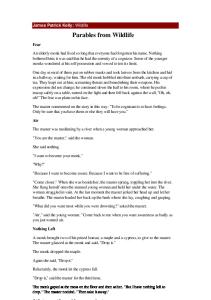
Figure 4.1. Time-series for annual census of adult population in six avian species, (a) Great tit (Paras major); (b) blue tit (Paras caeruleus); (c) tufted duck (Aythyafuligula); (d) grey heron {Ardea cinerea); (e) mute swan (Cygnus olor); (/) South Polar skua (Catharacta maccormicki).
duration of most ecological time-series reduces the statistical accuracy of such assessments (Lande etal. 2002). There are a autoregression coefficients and, from equations (4.3.2) and (4-3-3)) the product of the adult mortality rate and the total density dependence in the life history can be estimated, with reasonable accuracy, as one minus the sum of the autoregression coefficients, a
fiD = i-Y]bT.
(4.4.1)
Time-series were analysed for six avian populations with three or more decades of accurate annual census data and few missing observations (figure 4.1). Counts of the great tit (Parus major) and blue tit (Parus caeruleus) at Ghent, Belgium, and the tufted duck (Aythyafuligula) at Engure Marsh,
61
62
R.Landeefa/. Table 4.1. Bias-corrected estimates of total density dependence, D, with 95% confidence intervals in parentheses. (Population time-seriesfittedto the stage-structured life-history model - equation (4.3.3) - with age offirstreproduction a and annual adult survival rate s(= 1 - jl)) obtainedfrom the literature (Clobert et al. 1988; Dhondt et al. 1550; Blums et al. 1993,1996; Owen i960; North & Morgan 1979; Bacon & Andersen-Harild 1989; Bacon &?errins i99i;Jouventin &Guillotin 1979; H. Weimerskirch, unpublished data). **p < 0.01 for hypotheses thatjiD > o, by one-tailed test. CV, coefficient of variation; R2, proportion of total variance explained.) Species
Years
CV
a
AD
Rl
s
D
great tit
35
0.30
1
0.16
0.46
0.99
blue tit
35
0.26
1
0.15
0.49
0.99
tufted duck
36
0.27
1
0.14
0.65
1.61
grey heron
71
0.18
2
0-73
0.70
0.27
mute swan
116
0.26
4
0.80
0.85
0.41
35
0.16
5
0.535** (0.184,0.879) 0.507** (0.157,0.849) 0.564** (0.221,0.907) 0.081 (0.000,0.246) 0.062 (0.000,0.184) 0.397**
0.29
0.85
2.65
South Polar skua
(0.103,1-114)
Latvia, are for the total adult population (>i year old). Counts of the tits are almost exact since nearly all pairs breed in nest boxes, but there is considerable exchange of individuals with other populations. The grey heron (Ardea cinerea) counts are for the breeding adult population (>2 years old) in southern Britain, which therefore constitutes a relatively closed population. Counts of the mute swan (Cygnus olor) on the Thames, England, are for the total population minus fledglings. The time-series for the mute swan was truncated following a period of no data during World War II, after which large population increases occurred in both adults and yearlings (Cramp 1972). Some of the mute swan annual counts may be biased (Birkhead & Perrins 1986) and fledglings were wing-clipped during the counts to reduce emigration (Cramp 1972); this series is included mainly for illustrative purposes because of its length. The South Polar skua (Catharacta maccormickt) population at Pointe Geologie archipelago, Terre Adelie, Antarctica, has significant recruits from outside of the archipelago. The strong territoriality of adults helps to ensure that all birds in the archipelago are ringed
Estimating density dependence
and the counts of breeding adults are exact. Years without a complete census were excluded from the analysis of the mute swan and South Polar skua. Employing basic statistical methods for stationary autoregressive timeseries analysis, we found evidence of density dependence in four out of the six species (table 4.1). Although the theory indicates that the noise in the population process may be autocorrelated - see equation (4.3.3) - so that, using life-history information, the population time-series could in principle be analysed as an autoregressive moving average process (ARMA, cf. Box et al. 1994), residuals from the simple autoregression showed no significant autocorrelations in the noise, justifying the approximation of independent errors in estimation and significance testing. 4.5.
Discussion
Turchin (1990,1995), Royama (1992), Turchin & Taylor (1992), Zeng et al. (1998) and others fitted nonlinear autoregressive models with time-lags of one, two or three years to population time-series. They interpreted a significant autoregression coefficient for a time-lag greater than one year as evidence for density dependence with a time-lag. However, their models are phenomenological and not based on explicit demographic mechanisms. Our results - see equation (4.3.3) - demonstrate that the interpretation of autoregression coefficients is clarified by deriving the form of the linearized autoregressive equation from a nonlinear stochastic lifehistory model. In the stage-structured model, density dependence operates with time-lags up to a years. Contrary to previous interpretations, the autoregression coefficients do not directly measure density dependence operating at particular lags. The autoregressive coefficients depend on parameters of the life history as well as density dependence of a particular stage class. It is instructive to consider a species with a = 1 and autoregression coefficient 6, = o, which implies that all autocorrelations are zero (except po = 1), corresponding to a flat power spectrum or white noise process for the population. This would entail very strong density dependence, D = i/A (the inverse of the adult annual mortality rate), despite the regression explaining none of the total variance, Rz = o. The tufted duck approaches this situation, having a low R2 (table 4.1). Thus, statistical significance of autoregression coefficients is not a valid criterion for the detection of density dependence.
63
64
R. Lmdc etal.
Total density dependence in the life history was significant in four out of the six species. Comparing the strength of total density dependence, D, between species requires correcting the estimates of AD in table 4.1, through division by the adult annual mortality rate, A- In conjunction with the estimates of [MD derived from autoregression analyses, adult annual survival rates s(= 1 - A) obtained from life-history studies allow estimation of the total density dependence, D, in each of the populations (table 4.1). Strong density dependence occurs in each of the four populations in which significant estimates were obtained. Density dependence for the grey heron and the mute swan, which had the longest time-series, is relatively weak and not significant. The average value of the total density dependence in the six species is D=1.16. Thus, on average, a given proportional increase in adult population density, N, produces roughly the same proportional decrease in multiplicative growth rate of the population per generation, XT. Because the expected annual rate of return to the equilibrium population size is y = D/T, stochastic perturbations from the equilibrium population size for the bird species analysed here all appear to have o < y < 1 and thus to be undercompensated (Begon etal. 1996c, pp. 239-240), since even for species with age of maturity equal to one year the generation time is generally larger than D. Autocorrelation of physical and biotic environments has been discussed as a cause of autocorrelated noise (Williams & Liebhold 1995; Berryman & Turchin 1997). The present theory reveals that environmental covariance in vital rates, operating at different time-lags, creates another source of autocorrelated noise, even in the absence of environmental autocorrelation - see equation (4.3.3). Observed correlations among vital rates (Ssether & Bakke 2000) may be caused both by environmental covariances and by density dependence in the vital rates. Long-term life-history studies of vertebrate species often show that estimates of recruitment of yearlings (reproduction multiplied by first-year survival) are much more variable among years than estimates of adult mortality (Gaillard etal. 1998, 2000; Sasther & Bakke 2000), as observed in the tufted duck (Blums et al. 1996), grey heron (North & Morgan 1979) and mute swan (Cramp 1972; Bacon & Perrins 1991). This would tend to reduce the environmental covariance of vital rates in the stage-structured model - see equation (4.3-3)The present autoregression analysis, like previous studies (see, amongst others, Turchin 1990,1995; Royama 1992; Turchin & Taylor 1992; Zeng etal. 1998), assumes no autocorrelation of the noise. Residuals from the autoregressions showed no significant autocorrelations, suggesting not only
Estimating density dependence
a negligible environmental autocorrelation, but also that environmental covariance of vital rates operating at different time-lags is small. Timeseries of at least an order of magnitude longer than the number of autoregression coefficients are required to estimate accurately the total density dependence. Our results illustrate the advantages of applying demographic theory both to define the total density dependence quantitatively in a life history and to estimate it from population time-series. We are grateful to Andre Dhondt, Jenny De Laet and Frank Adriaensen for providing the great tit and blue tit data, the British Trust for Ornithology for providing the grey heron data and Henri Weimerskirch for providing the South Polar skua data. This work was supported by National Science Foundation grant DEB 0096018 to R.L. and by grants to B.-E.S. and S.E. from the Research Council of Norway.
65
BERNT-ERIK SSTHER AND STEINAR ENGEN
Pattern of variation in avian population growth rates
5.1.
Introduction
Studies on population growth rates (i.e. how fast population size changes) go back several hundred years, at least to the 16th century when the potential for exponential growth of populations was realized (Caswell 2001). Since then, factors affecting variation in population growth rates have been the major focus for human demography and a major part of population ecology. Although ecologists have dealt with this problem for a long time, surprisingly few generalizations have appeared that allow us to predict variation in population growth rates within and among natural populations. A major reason for this may be difficulties in separating out the relative contribution of density-dependent and density-independent factors on the population growth rate (see reviews in Sinclair 1989; Caughley 1994; Turchin 1995). The purpose of the present study is to summarize how stochastic effects affect the long-term growth rate of populations with no age structure. We will then extend some recent work (Satther etal. 2002), using data on fluctuations of bird populations, where stochastic factors as well as parameters characterizing the expected dynamics are being separately estimated. We suggest many characteristics of avian population dynamics are closely associated to variation in the specific population growth rate because of the presence of covariation between differences in the expected dynamics and the stochastic component of the fluctuations in population size. Finally, we strongly emphasize that reliable population projections, for example for use in population viability analysis, will not only require estimates and modelling of the expected dynamics as well as the
[66]
Variation in avian population growth rates
stochastic components, but also assessment of the effects on the predictions of uncertainties in parameter estimates. 5.2.
Stochastic population growth rates
To illustrate the importance of stochastic effects on population dynamics, we consider a simple model describing density-independent growth in a random environment N(t +1) = X(t)N(t) (Lewontin & Cohen 1969). Here N(t) is population size in year t, and X(t), the population growth rate in year t, is assumed to have the same probability distribution each year with mean X and varianceCT*.If the population size is sufficiently large to ignore demographic stochasticity, the environmental stochasticity is al = ol = var (AN/N | N), where AN is the change in population size between t and t + 1. Population ecologists commonly analyse population fluctuations on the natural-log scale (Royama 1992) so that X (t + 1) = X(t) + r (t), where X (t) = In N (f) and r(t) = In X(t). If E denotes the expectation, the growth rate during a period of time t, (X(t) - X(o))/t, has mean s = Er and variance var(r)/t = o\lt. For long time intervals the mean slope of the trajectories on log scale all approaches the constant 5, which is called the stochastic population growth rate. This leads to the approximation s « I n X - Or/i and 0? « af/X1 = crf/X2- for the mean and the variance, respectively (Lande et al. 2003). As expected, we see by simulating this model that all sample paths are after some time below the trajectory for the deterministic model (figure 5.1). Stochastic effects reduce the mean growth rate of a population on the logarithmic scale by ca. o?/2, compared with one in a constant environment. Demographic stochasticity is caused by random fluctuations in individual fitness, which are independent among individuals, giving var(AN/N | N) = a} + cr^/N (Engen et al. 1998; Szther et al. 1998), where aj is called the demographic variance. It produces a similar reduction in the stochastic growth rate s as the environmental variance a}, given by
(Lande 1998). We see that at small population sizes demographic variance creates a deterministic decrease in the long-term growth rate in addition to causing random fluctuations in population size so that var(AN | N) = alW +CTrf2N.However, for population sizes of N » ollol environmental
67
68
B.-E. Ssether & S. Engen
20-
IS-
50
100
150 time
200
250
Figure s.i. Simulation of five populations growing density independently in a random environment, with parameters r = 0.06, a, = 0.05 and initial population size No = 20. Solid line shows the population growth in a constant environment and the dashed line the expected long-run growth.
stochasticity constitutes the major contribution to stochastic variation in the rate of population growth. One of the few general patterns in ecology is the dependence of population growth rates on population size (Turchin 1995). In the density-dependent case, the population growth rate at population size N is rN = E(AN/N | N) = E[(X -1) | N)] on an absolute scale, and 5N = E(A In NIN) = E(r | N) on a logarithmic scale. To quantify the effects of density dependence on the population growth rate we use the thetalogistic model (Gilpin & Ayala 1973),
K
(5.2.2a)
where r0 is the mean specific growth rate of the population at N = o, K is the carrying capacity and 6 specifies the density regulation. We can also formulate (5.2.2a) as (5.2.2b)
(Ssether etal. 2000a), where r, is the mean specific growth rate of the population at N = 1. We can then describe a wide variety of density regulation functions by varying only one parameter 6 (figure 5.2). For instance, for 0 = o we get the Gompertz form of density regulation, whereas 9 = 1 gives the logistic model (figure 5.2).
Variation in avian population growth rates
Figure 5.2. The expected change in population size N from time t to t +1, conditioned on N (E( AN | N)) as function of relative population size (to the carrying capacity K) for different values of 6 in the theta-logistic model. Other parameters are rt = 0.1 and K = 100.
The dynamic consequences of variation in r, are strongly dependent on the density regulation function (figure s.3a,b). For a given r,, the variability decreases with increasing 9. Similarly, an increase in r, also reduces population variability if 9 is kept constant. This is due to the inverse of the rate of return to the equilibrium at the carrying capacity being Y=ro9=r1e/{i~K-e).
(5.2.3)
Thus, for a given 9, y will increase with r, and the population will return to equilibrium more rapidly (May 1981b). One advantage of the theta-logistic model is that it has relatively well understood statistical properties (Gilpin et al. 1976; Saether et al. 1996, 2000a; Diserud & Engen 2000). This allows us to calculate approximately the stationary distribution of population size. The variance of this distribution using the diffusion approximation (Karlin & Taylor 1981) is (5-2-4)
where a = zrja^i — K ") — 1, and F denotes the gamma function (Diserud & Engen 2000). The variance o^ is strongly influenced by af and 9 (figure 5.3c). Furthermore, for small values of 9 variation in rl strongly affects the stationary distribution of population sizes (figure 5.4), whereas smaller effects on a^ of variation in rt occur for larger 9.
69
70
B.-E. Ssther&S.Engen
200 •
150
100 •
50 •
50
0.2
0.4
0.6
100 time
0.8
1.0
150
1.2
1.4
1.6
1.8
2.0
e Figure 5.3- Ten trajectories of the population fluctuations during a period of 200 years in the theta-logistic model for (a) 9 = o.i and (b) 0 = 1.5, assuming or* = 0.01. (c) The variance in the stationary distribution of population size (o^) in relation to 9 for af = 0.01 and af = 0.1.
Variation in avian population growth rates
/ o
\ \
\.
i ~N (9 = 0 \ i \ / \ i 9=\ i \ \ \
r l iL
fre que
a
/A. /
/ 7s\
1 / I
\
\
/,7/
50
100 N
150
200
Figure 5.4. The stationary distribution of population sizes in the theta-logistic model - see equation (2.20,6) - for the Gompertz (9 = o) and logistic {8 = 1) type of density regulation for r, = 0.025 (solid lines) and r, = 0.1 (broken lines). Other parameters are K = 100 and a$ = 0.01.
When demographic stochasticity is present, there is no stationary distribution. For a} > o, we may compute approximately the quasistationary distribution, again using the diffusion approximation (Lande etal. 2003). A larger proportion of the distribution lies closer to zero in the quasi-stationary than in the stationary distribution obtained assuming oj = o (figure 5.5). Ignoring demographic stochasticity may thus cause serious underestimation of the time to extinction. Although variation in population growth rates strongly affects the characteristics of the population dynamics, surprisingly little is known about how, for example, rt varies among or within species. This may be related to difficulties in estimating r, due to the fact that reliable estimates of population growth rates require precise estimates of population size. Uncertain population estimates will lead to over-estimates of r, (Solow 1998) as well as the environmental variance. Furthermore, unbiased estimates of population growth rates are also difficult to obtain because many populations fluctuate around K so the population is rarely found at such small population sizes that the growth is close to r, (Aanes et al. 2002). In addition, large uncertainties will be present in the estimates ofK in many timeseries that in a statistical sense are short (Myers et al. 2001). This makes it even more difficult to obtain reliable unbiased estimates of r, because rt and K act together on E(AN/N | N) in (5.2.26).
B.-E. Sxther & S. Engen
50
100
150
200
N Figure 5.5. The estimated quasi-stationary (broken line) and stationary (solid line) (ae = o) distributions of the theta-logistic model. The population parameters are 9 = 0.5, r1 = 0.1, K= 100, a? = 0.01 and of = 1 (for the quasi-stationary distribution).
5.3. Density-independent population growth First, we consider some populations that have strictly declined or increased in size over a period of at least 10 years and where the population counts are assumed to be relatively precise (table 5.1). We estimate the stochastic population growth rate s and af according to Engen & Ssether (2000), following Dennis etal. (1991). When comparing only declining or increasing species, we still find large interspecific variation in s (table 5.1). The most dramatic decline (table 5.1) was recorded in a population ofPluvialis apricaria in Scotland (Parr 1992). By contrast, Branta leucopsis at the Island of Gotland in the Baltic Sea was the most rapidly increasing population in the dataset, with 5 = 0.285 (table 5.1). There was a positive relationship between the specific growth rate r and In orr2 among the species in the dataset (figure 5.6, correlation coefficient = 0.48, p = 0.029, n — 21). However, this relationship may be strongly influenced by sampling errors in the parameter estimates. To account for this we performed a meta-analysis (Hunter & Schmidt 1990), a technique that is currently becoming increasingly popular among comparative biologists (e.g. Arnqvist & Wooster 1995). We assume that r and In oy2 are binormally distributed among species. For populations that are not density regulated, it follows from standard normal theory (Kendall &
Table 5.1. Characteristics ofstrictly declining or increasing species included in the present study. (s is the stochastic growth rate and 0? = Vzr\inX{t)], where X(t) is the population growth rate in year t.) Species
Locality
Period
s
of
Source
Anas platyrhynchos Aptenodytesforestri Branta leucopsis Bubulcus ibis Cicconia cicconia Cicconiacicconia Cicconia cicconia Cicconia cicconia Cicconia cicconia Circus aeruginosus Diomedea exulans Gymnogyps californianus Haliaeetus albicilla Hirundo rustica Milvus milvus Otis tarda Pandion haliaetus Perdixperdix Phalacrocorax aristotelis Phalacrocorax carbo Phalacrocorax carbo Pluvialis apricaria Recurvirostra avosetta Sula bassanus
Engure Lake, Latvia Terre Adelie, Antarctica Gotland, Sweden Camargue, France Bohmen and Mahren, Czech Republic Estonia Denmark Netherlands Baden-Wiirttemberg, Germany Britain Bird Island, South Georgia California, USA Germany Jutland, Denmark central Wales Brandenburg, Germany Scotland Sussex, England Isle of May, Scotland Vors0, Denmark Ormso, Denmark northeast Scotland North Sea coast, Germany Alisa Craig, Ayrshire, Scotland
1958-1993
0.094 -0.014 0.285 0.267 0.071
0.152 O.O26 O.O65
Blums etal. (1993) H. Weimerskirch (personal communication) K. Larsson (personal communication) H. Hafner (personal communication)
0.034 -0.074 -0.068 -0.054 0.057 -0.006 -0.077 0.044 -0.076 0.040 -0.076 0.126 -0.058 0.146 0.116 0.206 —0.176 0.091 0.0269
O.O15
1952-1999 1976-2001 1967-1998 1930-1984 1939-1981 1952-1971 1929-1981 1950-1965 1927-1982 1962-1996 1965-1980
1976-1997 1984-1999 1951-1980
1975-1995 1958-1994 1970-2000 1946-1992 1978-1993 1978-1993 1973-1989 1951-1994
1936-1976
0.375 O.O34 O.O12 O.O9O 0.017 O.294 O.O1O O.12O O.OO3 O.O24 O.OO8 O.O12 0.027 O.O69 O.118 O.Oll O.O55 0.134 O.O68 O.OO4
Hladik(i986) Veromann (1986) Skov (1986) Jonkers (1986) Engen & Sxther (2000) (from Bairlein & Zink 1979) Underhill-Day (1984) Croxall etal. (1997) Dennis etal. (1991) Hauff(i998) Engen etal. (2001) Davis & Newton (1981) Litzbarski & Litzbarski (1996) Dennis (1995)
Aebischer (personal communication) Harris etal. (1994) Van Eerden & Gregersen (1995) Van Eerden & Gregersen (1995) Parr (1992) Halterlein & Sdbeck (1996) Nelson (1978)
74
B.-E. Sxthet & S. Engen
0.4 •
0.3 • 0.2 • 0.1 •
0-0.1 -5
-4
-3
-2
-1
MO Figure 5.6. The logarithm of the environmental variance a, in relation to the specific growth rate r, assuming no density regulation. Solid lines and circles represent the initial analysis, broken line and open circles the meta-analysis that takes into account uncertainties in the parameter estimates (see text). For sources, see table 5.1.
Stuart 1977) that the sampling errors in these two parameters are independent. The uncertainty in the estimate of r must be estimated from the data, whereas the variance in the estimate of In oy2 only depends on the sample size and can be calculated theoretically using well-known properties of the ^-distribution. Finally, assuming that the sampling errors are approximately normally distributed, we calculated the conditional expectation of the values for each single species, conditioning on the raw estimates. The results of these adjustments of the estimates are shown in figure 5.6. The estimated correlation in the bivariate between-species model was 0.49, with significance level p = 0.0580 calculated by parametric bootstrapping. This therefore suggests the presence of an interaction between the expected dynamics and the stochastic component of the population fluctuations. Overall, a large proportion of the variation in the stochastic population growth rate s was explained by differences in r (correlation coefficient = 0.95, p < 0.001, n = 21). However, the stochastic contribution to s differed between declining and increasing populations. In declining populations, oy2 contributed significantly to the variation in 5 (correlation coefficient = -0.66,p = 0.039, n = 10), whereas no such significant effect was present in increasing species (correlation coefficient = 0.40, p > 0.2, n = 11). This shows that not only the expected dynamics, but also quantifying the
Variation in avian population growth rates
stochastic effects are important for predicting the rate of decline in such decreasing populations. Variation in s among populations was not significantly (p > 0.2) related to differences in life history (clutch size or adult survival rate), either in declining or in increasing species.
5.4. Density-dependent population growth Traditionally, population ecologists have analysed population dynamics by fitting autoregressive models to time series of fluctuations in population size (Bj0rnstad & Grenfell 2001). Linearity at a logarithmic scale is often assumed (Royama 1992). Here, we take an alternative approach by estimating the parameters in the theta-logistic model (equation (5.2.20,6)) by maximum-likelihood methods (see Sxther et al. (2000a) and Saether & Engen (2002b) for a description of the methods). This enables us to estimate the form of the density regulation (see figure 5.3c). In 11 populations where 0 > o, the estimates of 6 ranged from 0.15 to 11.17 (table 5.2). This implies that the assumption of log-linearity (0 = o) is not necessarily fulfilled in time-series of fluctuations of bird populations (e.g. Sasther et al. 2002). Large uncertainty was found in most estimates of^ with wide confidence intervals of X, = exp(rt) in several species (figure 5.7). This shows that r, (or A,) is often difficult to estimate even in comparatively long time-series of population fluctuations. Even though we find large uncertainties in the estimates, a pattern of covariation appeared among several parameters of the theta-logistic model. As in the density-independent cases (figure 5.6), the environmental variance increased with r: (figure 5.80, correlation coefficient = 0.75, n = 11, p = 0.008). Furthermore, the logarithm of 6 decreased with r, (figure 5.86, correlation coefficient = -0.69, n = 11, p = 0.018), showing that maximum density regulation occurs at lower relative (to K) population sizes in species with higher population growth rates. The estimates of y, the strength of density regulation at K (equation (5.2.3)) also increased with al (figure 5.8c, correlation coefficient = 0.61, n = n,p = 0.048). We then examined how variation in the parameters affected interspecific variation in the variance of the stationary distribution (see equation (5.2.3)). Differences in o^ w e r e o n i y significantly correlated with al (correlation coefficient = 0.62, p = 0.043, n = 11). The interspecific variation in r, was also correlated with life-history differences. Lower growth rates were found in species with high survival
75
Table 5.2. Estimates ofparameters in density regulated bird populations. (r, specific growth rate; 6, theformat density regulation; af, environmental stochasticity; y, strength of density dependence at the carrying capacity, K.) Species
Locality
Period
r,
Ansercaerukscens Aythyaferina Ckconia dcconia Haematopus ostrakgus Lagopus lagopus Melopspiza melodia Parus caeruleus Phalacrocorax aristotelis Phalacrocorax carbo Recurvirostra avosetta Rissa tridactyla
Perouse Bay, Canada Engure Lake, Latvia Bbhmen and M'ahren, Czech Republic Mellum, Germany Kerloch, Scotland Mandarte Island, Canada Braunschweig, Germany Isle of May, Scotland Vorso, Denmark Havergate, England North Shields, England
1970-1987 1970-1987 1962-1984 1946-1968 1963-1977 1975-1998 1964-1993 1946-1992 1978-1993 1947-1986 1949-1984
0.09 0.82 0.09 0.74 1.50 0.99 1.16 0.55 0.17 1.04 0.17
e 2.05 0.15 3-74 O.65 0.47 1.09 0.54 0.33 11.17 O.25 2.05
ol
Y
Source
0.041 O.276 0.014 0.065 O.411 O.437 O.114 0.072 O.OO5 0.104 0.014
O.58 O.82
Cooch & Cooke (1991) Blums etal. (1993) Hladik(i986) Schnakenwinkel (1970) Moss & Watson (1991) Ssether etal. (2000a) Winkel (1996) Harris etal. (1994) Van Eerden & Gregersen (1995) Hill (1988) Porter & Coulson (1987)
O.37 O.56
1.94 2.25 1.50 O.36
2.10 O.39 0-37
Variation in avian population growth rates
Figure 5.7. The bootstrap replicates of the estimates of population growth rate X, = exp(r,) for the populations listed in table 5.2. {a)Ansercaerukscens; (b)Aythya ferina; (c) Cicconia cicconia; (d) Haematopus ostrakgus; (e) Lagopus lagopus; (f) Melospiza melodia; (g) Parus caerukus; (h) Phalacwcorac aristotelis; (1) Phalacrocorax carbo; U) Recurvirostra avosetta; (k) Rissa tridactyla.
77
78
B.-E. Saether & S. Engen
0.4 0.3 0.2 0.1
0
0.2
0.4
0.6
0.8
1.0
1.2
1.4
0.8
1.0
1.2
1.4
r 3
21 0-1 -
0
0.2
0.4
0.6 ri
(c)
2.52.01.51.00.50
0.1
0.2
0.3
0.4
Figure s.8. (a) Environmental variance o/, (b) the logarithm of S in relation to the specific population growth rate r,, and (c) strength of density regulation at the carrying capacity y in relation to a}. For sources, see table 5.2.
rates (figure 5.9a, correlation coefficient = -0.71, n = 9, p = 0.031) and small clutch sizes (figure 5.9b, correlation coefficient = 0.68, n = 11, p = 0.021) than in species at the other end of this 'slow-fast continuum' (Saether & Bakke 2000).
Variation in avian population growth rates (a)
1.61.41.21.0
^-
0.8 i 0.6 0.4 0.2 0
0.4
0.5
0.6
0.7
0.8
0.9
adult survival rate
(b)
1.6-1 1.41.21.00.80.60.40.20 10 clutch size
Figure 5.9. The specific population growth rate r, in relation to (a) adult survival rate and (b) clutch size in density regulated bird populations. For sources, see table 5.2.
5.5. Predicting population fluctuations Population viability analysis has during the last decades become an important tool in the management of threatened or vulnerable species (see reviews in Beissinger & Westphal 1998; Groom & Pascual 1998) because it provides a quantitative assessment of the probability for a population to decline to (quasi-)extinction. Our analyses show that large uncertainties are often found in the estimates of important parameters for population viability analysis - analyses such as the form of the density regulation (Ssether etal. 2000a) and r, (figure 5.7), even in time-series of a length that
79
80
B.-E. Sxther & S. Engen
are rarely available in populations of endangered and threatened species. Predictions from population viability analyses must therefore take into account these uncertainties. Elsewhere, we have suggested (Sxther et al. 2000a; Engen & Ssether 2000; Engen et al. 2001; Sxther & Engen 2002b) that the concept of population prediction interval can be useful in such analyses, embracing the effects of the expected dynamics and stochastic factors as well as uncertainties in parameter estimates on future population trajectories. The population prediction interval is defined as a stochastic interval that includes the unknown population size with a given probability (1 - a). We define extinction to occur when N = 1. We then predict extinction in a sexual population to occur after the smallest time at which this interval includes the extinction barrier. The width of the population prediction interval increases with the process variance (Heyde & Cohen 1985) and the estimation error. It is important to notice that the uncertainty in the parameters does not change the extinction risk of the population, but it will affect the confidence we have in the population predictions, including the probability of extinction. We will illustrate our approach by an analysis of factors affecting the width of the population prediction interval in two populations of passerine birds. Many species of birds breeding in areas of Europe with a highly intensified agriculture have declined in numbers (Pain & Pienkowski 1997; May 2000; M0ller 2001). In a study of Hirundo rustica on Jutland, Engen et al. (2001) predicted the time to extinction of such a population that declined from 184 in 1984 to 59 pairs in 1999. The estimates of the population parameters were $ = -0.078, a% = 0.18 and of = 0.024, respectively. Ignoring uncertainties in the estimates, the width of the 90% population prediction interval included the extinction barrier after 28 years (figure 5.10a). Including uncertainties in the parameter estimates, this time was decreased by 25% to 21 years (figure 5.106). Furthermore, in studies of time to extinction the demographic variance is assumed to be zero. Ignoring the demographic variance, the upper 90% population prediction interval included extinction first after 33 years (figure 5.10c). This occurs because the lack of demographic variance fails to account for the acceleration of the final decline to extinction produced by demographic stochasticity (Lande et al. 2003). Similarly, in a widely fluctuating small population of Melospiza melodia in Mandarte Island accounting for uncertainty produced a more precautionary assessment of extinction than under the assumption of exactly known parameters (Sjether etal. 2000a). Again, using the upper 90%
Variation in avian population growth rates
40
50
Figure 5.10. The upper bounds of population prediction intervals for a declining population olHirundo rustica in Jutland, Denmark, when (a) assuming no uncertainty in the parameters, (6) including demographic and environmental stochasticity as well as uncertainties in the parameters, and (c) assuming no demographic stochasticity, of = o.
81
82
B.-E. Sasther & S. Engen
population prediction interval the shortest time in which the population prediction interval included the extinction boundary n = 1 was 17 years whereas with no uncertainty in parameter estimates this interval was increased to 30 years. 5.6.
Discussion
This study demonstrates a strong covariation among the specific growth rate r, and other parameters characterizing fluctuations of bird populations. Both in density-independent and in density-dependent models the population growth rate increased with the environmental variance al (figures 5.6 and 5.8a). Large uncertainties were found in most estimates of r, in the density-dependent populations (figure 5.7). However, a relationship still appeared between r, and the form of the density regulation, expressed by 9 in the theta-logistic model (figure 5.86). Thus, maximum density regulation occurred at larger densities (relative to K) in populations with a small r, than in populations with larger values of r,. A similar pattern has previously been noted by Fowler (1981,1988). Furthermore, populations most rapidly growing at smaller densities were more subject to random fluctuations in the environment than populations with smaller values of r, (figure 5.8a). A strong pattern of covariation occurs in avian life-history traits (Sxther 1988; Ssther & Bakke 2000; Bennett & Owens 2002), which can be considered as representing a 'slow-fast continuum' of life-history adaptations. At one end of this dimension wefindspecies that are reproducing at a high rate, but with a short life expectancy at birth. At the other end, species that produce a small number of offspring, mature late in life but have a high adult survival rate, are found. This study shows that in density regulated populations a large proportion of the variance in the specific growth rate r, can be explained by the position of the species along this 'slow-fast continuum' (figure 5.9). The specific growth rate was higher in populations with large clutch sizes and low adult survival rates than in less fecund species with long life expectancy at maturity. This is in contrast to fishes, where Myers et al. (1999) failed to identify any relationship between r, and any life-history characteristics. The difference among these two studies may be related to larger uncertainties in the estimates of r, in fishes than in birds. Furthermore, relative smaller interspecific variation in r, may also be present in fishes than in birds.
Variation in avian population growth rates
The covariation among the specific growth rate r,, environmental variance 200 persons km"2: 36)
i>? 3-
| g.
H 0 -1 50
100 150 200 250 300 350 400 450 500
population density (arable land) (100-200 persons km"2: 20)
loo
W. Lutz & R. Qiang
six Middle Eastern desert states because they greatly distort the picture with almost no arable land and rather significant populations mostly due to oil revenues. As the following results show, the two different measures of population density do not produce qualitatively much different patterns of association. The best density variable that one would like to measure in its impact on fertility is perceived density based on perceived living space as it influences behaviour, but we do not know of any data on this. The two density measures applied here cover presumably two important determinants of this perceived density and therefore in combination seem to be an acceptable proxy. For this analysis, time-series data from i960 to 2000 (infive-yearsteps) have been collected for 187 countries mostly derived from international sources (World Bank 2001; United Nations 2001; and see FAO statistical databases at http://apps.fao.org/subscriber/). These data include population size, the different population densities, annual population growth rates, total fertility rates, as well as female labour force participation rates, female literacy rates, urban proportions, GDP per capita in constant US$ and a food production index. Figure 6.3 depicts these data on the bivariate relationship between population density (arable land) (on the horizontal axis) and population growth rates (on the vertical axis). The lines connect the data of individual countries over time. In order to be able to discover some possible patterns among this massive amount of data, the figure sorts the countries according to their population density in i960 into five groups ranging from the lowest with less than 25 persons per square kilometre to the highest of above 200 persons per square kilometre. Aside from some country-specific peculiarities, the graph does not show any clear bivariate association between the two variables within each of the five groups, neither cross-sectionally nor over time. By comparing across groups, however, it is evident that the average population growth rate is lower for countries with higher density. Figure 6.4 plots the same country grouping of the time-series but replaces population growth rates with total fertility rates on the vertical axis. Here, a much clearer pattern of association appears. As population density increases over time the mean number of children tends to become
Figure 6.4. Bivariate relationship between total fertility rate and population density in five groups, according to i960 density, 1960-2000. (Note: a five-year perception lag for TFR has been assumed.) Each line corresponds to the time-series of one country; numbers at the end of x-axis labels give numbers of countries.
0 10 20 30 40 50 60 70 population density (arable land) (< 25 persons km"2: 37)
76543" 2"
7 6
543250 100 150 200 250 300 population density (arable land) (50-100 persons km"2: 20)
0
30 50 70 90 110 130 150 population density (arable land) (25-50 persons km"2: 16)
1000 2000 3000 10000 30000 population density (arable land) (>200 persons km"2: 38)
100 200 300 400 500 600 800 population density (arable land) (100-200 persons km"2: 22)
102
W. Lutz & R. Qiang
lower. Also, when comparing across groups, it is quite apparent that countries with higher population density have on average much lower fertility rates. Why is the picture so different with respect to the fertility rates than with respect to population growth rates? To interpret this we have to be aware of the fact that even in a population closed to migration, population growth rate is determined by three factors: fertility, mortality and population age structure. Of these three, only fertility is directly a consequence of changing individual behaviour; therefore, only fertility can reflect possible psychological reactions to increasing population density. During the process of demographic transition, mortality is typically positively correlated with fertility. As mortality rates go down and life expectancy increases, fertility rates also go down. This mortality decline counteracts the negative impacts of a fertility decline on population growth rate because more people stay alive, thus contributing to a higher population size. It is also worth noting that since the advent of modern preventive medicine and hygiene, human population density does not seem to have a positive association with the level of mortality as one might infer from animal ecology and considerations of carrying capacity. If there is an association, it seems to be a negative one, with urban areas almost universally showing lower mortality rates than rural areas. This even seems to hold in some of the most polluted megacities because the generally much better access to health facilities in urban areas seems to outweigh the negative environmental impacts. It is worthwhile to have a closer look at this apparently strong bivariate relationship between density and fertility because it might not really reflect a causal relationship, but rather could be due to some other developmental variables in the background, such as level of income or level of education that might simultaneously lead to lower fertility and make higher population densities possible. For this reason tables 6.3, 6.4 and 6.5 give sets of multiple regressions that study the relationship of population growth and fertility to population density while controlling some of the other social and economic variables measured. To get a more differentiated picture and to avoid serial autocorrelation, the regressions are given separately for the seven points in time and separately for the subset of developing countries, in order to rule out the possibility that the bipolarity between developed and developing countries dominates the appearing pattern. A perception lag of five years has been assumed between the explanatory and the dependent variables, i.e. the independent variables listed for i960 are being related to fertility and population growth in 1965, and so on. The calculations shown here are based on giving equal weight
Table 6.3. Multiple linear regressions ofseveral variables on the annual population growth rate (lagged byfiveyears)for 187 countries, 1960-1990.
Variable all countries (n = 187) female labour force participation rate population density female literacy rate population urban GDP per capita 1 food production index b R
2
i960 Standardized coefficients
-0.041 0.266* 0.139 -0.056 -0.076 -0.246 0.142
1965
Standardized coefficients
0.121
0.277* 0.102 O.273 -O.319 -0.122 0.122
1970 Standardized coefficients
1975
Standardized coefficients
1980 Standardized coefficients
1985
1990
Standardized coefficients
Standardized coefficients
-0.208
0.109
-0.079
0.057
-0.029
0.203 0.079 0.079 -0.171 -0.172 0.075
0.082 —0.196 0.108 -0.214 0.088 0.067
0.135 -0.105 0.165 -0.289* -0.257* 0.141
0.002 -0.127 -0.044 -0.195 -0.246* 0.163
-0.041
-0.139
0.074
0.004
—0.217
0.070 -0.180
0.068
0.133
-0.013 -0.099 -0.034 -0.233 -0.296* 0.172
-0.094 -0.179 -0.088 -0.210
0.110
0.124 -0.082 0.155 -0.294* -O.262*
-0.064 -0.172 -0.126 —0.098 -0.179 0.134
LDCs c (n = 143)
female labour force participation rate population density female literacy rate population urban GDP per capita1 food production index b R2
—0.105
O.O86
0.228 0.131 -0.087 -0.127 -0.239* 0.146
0.268*
0.185
0.1X1
0.076
a
O.224 -O.252 -0.102 0.110
0.018 -0.138 -0.160 0.068
0.049 -0.196
Constant 1995 US$ for GDP per capita. i989-i99i = 100 as reference for food production index. c Comprises all regions of Africa, Asia (excluding Japan), Latin America and the Caribbean plus French Polynesia. b
*p < 0.05; "p < 0.01; ***p < 0.001.
-0.174 0.177
Table 6.4. Multiple linear regressions ofseveral variables on the TFR (lagged byfiveyears) for 187 countries, 1960-1990.
Variable all countries (n = 187) female labour force participation rate population density female literacy rate population urban GDP per capita 3 food production index*1 R2
i960
1965
1970
Standardized coefficients
Standardized coefficients
Standardized coefficients
-0.167 -0.177 * -0.387" —0.024
—0.096 -0.191* -0.508*" -0.051 -0.389" -0.088 0.703
-0.146 -0.225* -0.510*" -0.274 -0.180 -0.062 0.612
-0.514*** -0.133 0.655
1975 Standardized coefficients
1980
1985
1990
Standardized coefficients
Standardized coefficients
Standardized coefficients
-0.085 -0.196" -0.601"* -0.106 -0.244* -0.019 0.710
-0.144 -0.226"
-0.153 -0.236*" -0.701*** -0.245* -0.018 0.028
-0.068 -0.248"* -0.618"* -0.261* -0.048 0.137*
0.714
O.734
—0.117 -0.239"' -0.629"* -0.275* -0.043 -0.026 0.712
-0.104 -0.229** -0.603*** -0.299 -0.011 0.011
-0.122 -0.245" -0.671*** -0.270* 0.033 0.060 0.660
-0.102 -0.264** -0.694"* -0.266* 0.074 0.074 0.684
-0.069 -0.281*" —0.607***
-0.025 -0.296*" -0.590"* -0.340* 0.076 0.124
-0.694*** -0.218 -0.051 0.015
0.698
LDCs c (n = 143)
female labour force participation rate population density female literacy rate population urban GDP per capita3 food production index b R2
-O.Z49 -O.193* -O.336** -0.243
-O.399* -O.145 O.567
3
0.637
Constant 1995 US$ for GDP per capita. i989—1991 = 100 as reference for food production index. c Comprises all regions of Africa, Asia (excluding Japan), Latin America and the Caribbean plus French Polynesia. b
*p < 0.05; **p < 0.01; *"p < 0.001.
-0.384** 0.087 -0.008
0.664
0.637
Table 6.5. Multiple linear regressions ofseveral variables (usingdensity as defined by arable land) on the TFR (lagged byfiveyears) for 181 countries, 1960-1990.
Variable all countries (n = 181) female labour force participation rate population density (arable land) a female literacy rate population urban GDP per capita b food production index c R2
i960 Standardized coefficients
1965 Standardized coefficients
1970
1975
1980
1985
1990
Standardized coefficients
Standardized coefficients
Standardized coefficients
Standardized coefficients
Standardized coefficients
-0.183 -0.184* -0.404** 0.305 -0.591*" -0.126 0.671
—0.100 -0.186* -0.518*"
-0.056 -0.162* -0.603"* 0.014 -0.372" 0.014 0.727
—0.141 -0.156* -0.696*** -0.060 -0.257* 0.023 0.727
-0.160
-0.102 -0.173"
0.738
—0.169 —0.196* 0.007 0.722
-0.057 -0.203" -0.622— -0.201*
-0.280 -0.276" -0.352" -0.204
-0.166 -0.266**
—0.109 -0.226* -0.626*** -0.192 -0.123 0.013 0.648
-0.164 -0.205*
-0.130 -0.193*
-0.068 -0.221"
-0.715"* -0.219
-0.734*"
-0.654***
-O.216 -0.009 O.087 0.666
-0.259 -0.004 0.015
0.034 -0.492*** -0.075 0.725
-0.153* -0.710*** -0.123 —0.210* 0.057
-0.643"*
-0.153 0.135* 0.704
LDCs d (n = 137)
female labour force participation rate population density (arable land) a female literacy rate population urban GDP per capita b food production index0 R2
-0.469* -0.154 0.615
-0.534*** -0.181 -O.289 -0.073 0.648
-0.037 0.042 0.650
includes land currently used for other purposes such as grassland, forests, protected areas, buildings and infrastructure, etc. b Constant 1995 US$ for GDP per capita. c i989-i99i = 100 as reference for food production index. d Comprises all regions of Africa, Asia (excluding Japan), Latin America and the Caribbean plus French Polynesia. *p < 0.05; " p < 0.01; ***p < 0.001.
0.659
-0.006 -0.250** -0.607*** -0.237 -0.033 0.136
0.639
io6
W. Lutz & R. Qiang 9876u. J 1
4 321 0
10
20
30 40 50 60 70 female literacy rate 15+
80
90
Figure 6.5. Bivariate relationship between literacy rates for females aged 15+ and total fertility rates for time-series of 65 developing countries, 1960-2000. Each line corresponds to the time-series of one country.
to all countries. Additional calculations based on a weighting of the countries by their population size yielded qualitatively similar results and are given in electronic Appendix A available on The Royal Society's Publications Web site. The results of these 28 multiple regressions cannot be discussed in detail here, but a few general conclusions can be drawn. In almost all regressions for the fertility rate, female literacy seems to be the single most important factor. This is consistent with the large body of literature on fertility determinants and with the theoretical foundations of the process of demographic transition described above. The tables show that the relationship of female literacy to the total fertility rate is more pronounced than that to the growth rates across all points in time. The urban proportion also has a consistent negative association with fertility (the higher the degree of urbanization, the lower fertility) but is not always statistically significant. GDP per capita only shows a significant negative coefficient with fertility during the 1960s on the global level, while it is insignificant with a variable sign in all the other regressions. With respect to population growth rates (table 6.3), the pattern and even the signs of the coefficients are much less consistent over time and are statistically insignificant in general. This has to do with the fact that changes in total population size are also influenced by mortality and migration, which tend to have less consistent associations with density. As a piece of background information, figures 6.5 and 6.6 plot the bivariate relationships of income and
Human population growth 9 -i
8 7 6 5 4 3 2 I 0
1000 2000 3000 4000
15000 30000
GDP per capita Figure 6.6. Bivariate relationship between GDP per capita (constant 1995 US$) and total fertility rate in 55 developing countries (same countries as in figure 6.5 with available income data), 1960-2000. Each line corresponds to the time-series of one country.
female literacy to the total fertility rate. The comparison of the two figures impressively confirms the view that female literacy is a much more straightforward and almost linear covariate (and determinant) of declining fertility than GDP per capita, where the picture is very mixed. How does population density - under both definitions used here come out as an explanatory variable in this multivariate setting? Again the relationship is much stronger and more statistically significant in the case of fertility as the dependent variable, although the signs are consistently negative for both fertility and the growth rate. When explaining the level of fertility, population density comes out second in importance after female literacy, yet still well ahead of the traditionally studied factors: female labour force participation, income, urbanization and food security. This strong negative effect of population density on the level of fertility five years later is statistically significant in almost all years, both at the global level and among the sub-group of developing countries. When comparing the results for the two definitions of density (see tables 6.4 and 6.5), the one based on arable land turns out to be slightly less significant than the one based on total area. In order to understand better the possible effects of population density on human fertility, more research is needed in terms of studying both these associations and sub-national scales, and in terms of understanding better the possible mechanisms of causation. For the former, table 6.6 gives a simple correlation analysis for the 30 provinces of China, which
107
Table 6.6. Correlation coefficients between population density (under three different definitions) and the TFR as well as population growth rate (lagged byfiveyears) in China's 30 provinces (numbers ofprovinces in parentheses), 1970-1990. (Sources of data: Yin Hua & Lin Xiaohong 1996; Population Census Office under the State Council et al. 2001; Fischer et al. 1998.) Variable
1970
1975
1980
1985
population density-population growth rate population density-TFR
-0.764** (30) -0.581" (28)
-0.294(30) -0.587** (28)
-0.103(30) - 0 . 5 5 6 " (30)
-0.346* (30) -0.529** (30)
population density (potential cultivated land)-population growth rate population density (potential cultivated land)-TFR
—0.629** (29) - 0 . 4 7 4 " (28)
—0.160(29) - 0 . 4 6 0 " (28)
—0.004(29) - 0 . 4 7 7 " (29)
—0.339* (29) - 0 . 4 7 9 " (29)
population density (currently cultivated land)-population growth rate population density (currently cultivated land)-TFR
- 0 . 7 4 6 " (29) -0.532" (28)
-0.254(29) -0.536** (28)
-0.019(29) -0.501** (29)
-0.316* (29) - 0 . 5 2 2 " (29)
*p < 0.05; " p < 0.01.
Human population growth
also confirms the above-described associations at a sub-national level for the world's most populous country, which has seen dramatic fertility declines over the past three decades. While the correlations between density and fertility are consistently high over time, the relationship to the growth rate is also affected by changing patterns of inter-provincial migration. As to the possible mechanisms of causation, direct biological factors such as decreasing fecundability due to 'density stress' are rather unlikely candidates for the human population, especially in a technologically advanced stage of development. Instead psychological factors, such as perceived living space, may play a role. An earlier study (W. Lutz, personal communication) identified a clear 'island factor' in the onset of fertility declines, i.e. the fact that in otherwise comparable socioeconomic settings, small islands - where the spatial limitations are obvious - began their fertility transitions earlier. But even with respect to contemporary European fertility levels, it is conspicuous that the very-low-density regions of northern Scandinavia have significantly higher fertility than the high-density areas of central and southern Europe. This clearly needs further investigation. In conclusion, we have shown that the process of demographic transition has led to unprecedented growth in the human population, but will also lead to significant population ageing and the likely end of world population growth. What will determine human population growth in the very long run, once the momentum of the demographic transitioninduced population growth comes to an end? This is an open question at this point. Biological and ecological factors will clearly be very important for the future human life span and health, but they may also play an increasingly important role with respect to human fertility. The section on past population growth draws partly from O'Neill etal. (2001). The section on future trends draws partly from Lutz etal. (2001).
109
CHARLES J. KREBS
Two complementary paradigms for analysing population dynamics
7.1.
Introduction
For more than 100 years, ecologists have been estimating populations of animals, beginning with those of economic value, and have tried to make sense of the resulting data. How to make sense of quantitative population data is not immediately clear. Once an ecologist has two successive estimates of population size, he or she follows the first law of quantitative ecology, which is to divide one number by the other, producing the finite population growth rate (X) that Sibly & Hone (Chapter 2) described. However, what to do next? This is the critical step. Being good scientists, most ecologists would wish to predict the size of the population growth rate and would proceed in one of two directions to do this. First, they could adopt the density paradigm of Sibly & Hone (Chapter 2) and plot population growth rate against population density. (The concept of a paradigm as promulgated by Thomas Kuhn (1970) has been used in many ways, and one might argue that the paradigms discussed here are better labelled as 'conceptual approaches'. I have no quarrel with this comment and I use the term 'paradigm' as shorthand for what ecologists do (cf. den Boer & Reddingius (1996).) Alternatively, they could adopt the mechanistic paradigm and plot population growth rate against an ecological factor, such as the amount of food available per capita, which may explain the change. What are the problems and what are the advantages of going in one direction rather than another? However, let us drop back for a moment to consider a whole set of assumptions that we have already made about our population. Many of these assumptions are discussed in other papers of this issue.
Two population regulation paradigms (i) (ii)
(iii)
(iv)
(v)
(vi)
We assume that we can define a population unambiguously. This can be a problem with open populations, We assume that we can measure population size accurately and can convert this to absolute population density. This is more difficult than many ecologists think, We assume that we have defined a biologically relevant time-step over which to measure the population growth rate. The time-step is not always obvious (Lewellen & Vessey 1998). We assume, at least initially, that all of the individuals in the population have equal impact, regardless of sex, age and genetic composition. We can relax this assumption later. We assume a uniformity of nature, such that whatever variable we can find to predict population growth rate will be the critical variable at other times and in other places. This assumption of repeatability is rarely tested, We assume that we can substitute time for space, or space for time, so that there is a uniform predictive function.
All of these assumptions operate within the equilibrium paradigm, and all of them are, potentially, hazardous if we assume a non-equilibrium world view in which transient dynamics are the rule rather than the exception. In this paper, I discuss primarily assumptions (iv)-(vi). Given that population ecologists must start somewhere, we admit to these assumptions for the moment and ask which direction to follow. 7.2.
Density paradigm
The density paradigm instructs our ecologist to plot population growth rate against population density. At this point, our ecologist might become suspicious because the same variable appears in both the x- and the 7-axis. However, we are assured by some biometricians that this is not a problem (Griffiths 1998) so we disregard this potential problem. If the density data are a time-series of one or more plots, much now depends on the trend shown by the data. If density is monotonically falling (or rising), it will not be possible to estimate the equilibrium point, except by extrapolation. If the population does not vary much in density, the relationship may well look like a shotgun pattern. The decision tree (figure 7.1) illustrates how to proceed. If there is a negative relationship between population growth rate and density, the next question is, which of the demographic components drive this relationship? Given that data are available to answer this question, the
m
112
C.J.Krebs is population growth rate related to population density?
no direct density dependence
z
test for delayed density dependence
try another paradigm
delayed density dependence
no delayed density dependence
what demographic components are related to density?
what factors cause these relationships? extrinsic •predation •food supply •disease •parasites •weather •landscape
intrinsic ksocial ^physiological • genetic
Figure 7.1. Decision tree for the density paradigm of population regulation.
next step is to find out which factors, or combinations of factors, cause these changes in births, deaths or movements (if the population is not closed). All of this is what I will call the standard analysis procedure of the density paradigm. What happens if there is no pattern in the plot of growth rate against density? We are assured by both theoreticians and empiricists (e.g. Nicholson 1933; Sinclair 1989; Turchin 1999) that there must be a negative relationship between population growth rate and density. If this is true, it raises an interesting question in respect of the relationship of theory in ecology to empirical data. If there must be a relationship, the problem of the field ecologist is to describe this relationship in terms of its slope and intercept. The problem is not to ask if indeed such a relationship exists (Murray 1999, 2000). There is no alternative hypothesis to test. The first strategy that is adopted after finding that there is no relationship between population growth rate and population density is to invoke delayed density dependence (Turchin 1990). This is a reasonable strategy because virtually every interaction in population ecology involves some time delays. However, this strategy opens a Pandora's Box because data analysis begins to take on the form of data dredging since we have no a priori way of knowing what the critical time delays might be. There are
Two population regulation paradigms
elegant methods of time-series analysis that can be applied to population data to estimate the integrated time-lags in a series of density estimates (Stenseth et al. 1998), but it is far from clear how to translate these estimated time-lags into ecological understanding. Do predators respond to changes in prey abundance instantly, via movements (e.g. Korpimaki 1994) or more slowly via recruitment processes (e.g. O'Donoghue et al. 1997; Eberhardt & Peterson 1999)? If delayed density dependence can be identified in a time-series of population densities, we can proceed in the same manner as the standard analysis procedure of the density paradigm and try to determine what causes these time-lags. The remaining problem is what to do with cases in which no direct or delayed density dependence can be identified in a time-series. In theory, this situation cannot occur, but it seems to arise frequently enough to cause endless arguments in the literature about the means of testing for direct and delayed density dependence (den Boer & Reddingius 1989; Dennis & Taper 1994). Most ecologists in this situation would not give up studying population regulation, but would switch to the second paradigm discussed by Sibly & Hone (Chapter 2), the mechanistic paradigm. 7.3.
Mechanistic paradigm
The mechanistic paradigm can be viewed in two ways. Sibly & Hone (Chapter 2) consider it an elaboration of the density paradigm, as shown in figure 7.1, and indicate that one can proceed to this level of analysis for populations that are well studied in a reductionist manner. Krebs (i995)j by contrast, viewed the mechanistic paradigm as an alternative to the conventional approach through the density paradigm. The mechanistic paradigm short-circuited the search for density dependence, on the assumption that no predictive science of population dynamics could be founded on describing relationships between vital rates and population density without specifying the ecological mechanisms driving these rates. The key question seems to be whether any density-dependent relationship is repeatable in time or space. I have been able to find few ecologists who have asked this question. The most well-studied groups in this regard might be commercialfishes,birds and large mammals. The Pacific salmon fisheries of western North America are managed partly on the basis of Ricker curves, which plot stock versus recruitment and are another form of a plot for density dependence. The clear conclusion from much research
113
114
C.J.Krebs 2.5-,
2.0-
1.5JS
1.00.5-
50
100
150
200
250
escapement (thousands) Figure 7.2. Non-repeatability of the relationship between population density and rate of population growth for Columbia River chinook salmon (Oncorynchus tshawytscha) over time. You could not manage this fishery in the 1950s using the relationship from the 1940s; this was because both oceanic and freshwater environments had changed. Upper curve illustrates data for the period 1938-1946; lower curve illustrates data for the period 1947-1959. (Data from Van Hyning 1974.)
work is that these Ricker curves cannot be specified as a fixed relationship either temporally, in the same river system, or spatially, between different rivers (Walters 1987). Figure 7.2 gives one illustration for a Chinook salmon stock from the Columbia River system. The Ricker curve for this salmon stock has changed over time, which is not surprising since there has been so much human influence on this river system that many extrinsic environmental factors, as well as intrinsic factors (Ricker 1982), have changed over time. Considerable work on bird populations allows us to test whether density-dependent relationships are repeatable over time and space. Both (2000) reviewed studies on density dependence in clutch size in passerine birds and found that, for the great tit (Parus major) in Europe, only 12 out of 24 long-term studies showed significant density dependence in clutch size. So even within the same species, there is no consistency of density dependence among different populations. Moreover, even in those areas with density-dependent clutch size, no consistent relationship applied to all areas (figure 7.3). This means that one cannot use the data from one area to predict what to expect in another area - density dependence is area-specific. The conclusion is that density-dependent relationships occur often but are not repeatable and are an unreliable basis for a predictive ecology.
Two population regulation paradigms 12-1
II109876
0
0.2
0.4
0.6
0.8
1.0
1.2
1.4
density (pairs ha"1) Figure 7.3. Non-repeatability of the density-dependent relationship between clutch size and population density for great tits {Parus major) in three woodlands in the Netherlands. You cannot use the density-dependent relationship from one area to predict clutch size in another area. Circles, Hoge Velue A; triangles, Vlieland; squares, Hoge Velue B. (Data courtesy of Both 1998.)
what demographic components are related to population growth rate?
what factors cause these relationships?
social physiological genetic •parasites •weather •landscape
Figure 7.4. Decision tree for the mechanistic paradigm of population regulation. The key difference from figure 7.1 is that we ask what demographic factors are related to population growth rate, not population density.
Figure 7.4 illustrates theflowdiagram for the mechanistic paradigm. It looks identical tofigure7.1, but has one very significant difference: instead of asking what demographic components are related to population density, it asks which are related to population growth rate. In cases in which
115
n6
C.J.Krebs
density is closely related to population growth rate, there will be no difference between these two approaches. However, in every non-equilibrial system, the differences can be very large. The critical assumption again depends on whether there is an equilibrium point for the system under study. The mechanistic paradigm is best adapted to short-term considerations in which questions about ultimate equilibrium states are not particularly relevant. It is closely related to the approach to population dynamics typified by the Leslie matrix (Caswell 1989). The mechanistic paradigm asks how individual animals are influenced by the factors affecting density and recognizes that individuals vary in their responses to predators, food supplies, parasites and weather, as well as in their social standing within the population. Behavioural ecology has made a particularly strong contribution to our understanding of individual differences and is pushing strongly to utilize this understanding to enrich population dynamics. Let us consider four case studies in order to contrast the density paradigm with the mechanistic paradigm.
(a) Fire ants Thefireant (Solenopsis imicta) is an introduced pest in the southern United States. It occurs in two forms, a monogyne form with a single queen and a polygyne form with multiple queens per nest. Monogyne fire ants are territorial, whereas polygyne fire ants are non-territorial and reach much higher average densities (Tschinkel 1998). Adams & Tschinkel (2001) carried out a removal experiment in an area of Florida occupied by the monogyne form. They removed all fire ant colonies from a circular core area with a radius of 18 m and then followed the recolonization for a period of five years (figure 7.5). Recolonization was rapid and ant biomass returned to control (equilibrium) values within two years, illustrating a density compensation driven by territoriality. Adjacent ant colonies expanded and new colonies arose from the dispersal of new queens. Population biomass in this area varied slightly from year to year (coefficient of variation of density 13%), but was on average quite stable. This experiment illustrates very well the standard analysis procedure of the density paradigm, which works well in this fire ant system. It also illustrates the mechanistic paradigm because the population carrying capacity was set by territoriality among colonies.
Two population regulation paradigms 800 n V 600-
o
400
200-
removal area
1991
1992
1993
1994
1995
1996
Figure 7.5. Density convergence experiment on the monogynous (territorial) form of the fire ant Solenopsis invicta in Florida. All colonies in core areas of 1018 m2 were removed from six plots in the spring of 1991. Recolonization was followed by measuring spring biomass of ants in each of the next five years. Convergence was 60% after one year and complete after two years, demonstrating density regulation back to the average control density of 613 g per 1018 m2 measured on six unmanipulated plots. The dotted line shows the average control ant biomass. Control biomass showed a coefficient of variation of 13%. (Data from Adams & Tschinkel 2001.)
(b) Song sparrows The song sparrow (Melospiza melodia) on Mandarte Island, British Columbia, has been the subject of a long-term study since 1962 and has been reported by Smith & Arcese (1986), Arcese & Smith (1988), Smith (1988) and many others. Figure 7.6 illustrates the population density changes in the song sparrow on this 6 ha island since 1975. The population trend consists of periods of three to four years of population growth followed by a catastrophic 1-year decline, and this has been repeated three times in the last 25 years. The first two of these population declines were correlated with severe winter weather; the third was not. Arcese & Smith (1988) showed that fledgling production declines at high density in this population, and these demographic symptoms could be relieved by adding food to territories. This population shows a clear difference between the density and the mechanistic paradigms. If we ask what prevents population increase, we answer that reproductive output is reduced as density increases and the mechanism limiting reproductive output is food shortage. If we ask what causes the largest changes in population growth rates, we answer that the major or key factor is severe winter mortality. The population trace of this species is the net result of negative
"7
118
C.J.Krebs
604020-
1976
1980
1984
1988
1992
1996
2000
year Figure 7.6. Density of song sparrow {Melospiza melodia) females on Mandarte Island, British Columbia, 1975-2001. Data courtesy of J. N. M. Smith and P. Arcese. The dashed line is the logistic equation fitted to these data by Saether et al. (2000a) and is clearly a very poor descriptor of the population trace. Female density is given per 6 ha.
feedback of high density on reproductive output and occasional major winter mortality. Does this population have an equilibrium density? We can ask what would happen to this population if there were no winter losses. The answer to this question is hypothetical and problematic because none of the identified density-dependent relationships does more than slow down the rate of population increase; they do not set it to zero (Arcese & Smith 1988). To complicate the matter more, this island is part of a metapopulation of song sparrows in the general region and while immigration is rare, it is critical for the maintenance of genetic diversity and for recovery from low numbers (Smith et al. 1996). Recent analyses (P. Arcese and J. N. M. Smith, personal communication) suggest that immigrants strongly affect the population growth rate because their outbred offspring have much higher survival and reproductive rates compared with birds with no immigrant genes in their lineage. The key to winter losses seems to be the genetic quality of individual birds. To summarize, the song sparrow on Mandarte Island is a very well-studied bird population and we have a good understanding of its population dynamics, which can be well described by both the density and the mechanistic paradigms. If, for some reason, we had to manage this population, we would try to manipulate the level of outbreeding to maintain high individual quality. Density dependence in this population does not prevent instability.
Two population regulation paradigms 0.9-1
v.y
a
uO.8a ^ ^
2 •3 0.7-
lo.6-
A °
^0.50.40
0.70.6-
0
o. -^
(b)
0.8-
5 10 15 20 25 30 35 population density
0.50.4 0.6 0.8 1.0 1.2 1.4
1.6
population growth rate
Figure 7.7. Relationship of annual adult survival rate to (a) population density and (b) population growth rate (A) for house sparrows {Passer domesticus) on four islands in Hegeland, north Norway, 1993-1996 (circles, Gjxr0y; squares, Infre Kvaroy; triangles, Ytre Kvar0y; diamonds, Hestmannoy). The density paradigm would expect adult survival rate to fall as population density rose. However, the opposite was observed. (Data from Sather et al. 1999.)
(c) House sparrow Sasther et al. (1999) have analysed the demography of the house sparrow (Passer domesticus) on four islands off north Norway over a period of four years. They were particularly interested in metapopulation dynamics, but their detailed studies allow us to ask how well we can understand their results with the approach suggested by the density paradigm. Saether et al. (1999) measured breeding population density by direct enumeration, and, from 1993 to 1996, estimated reproductive success (number of offspring fledged per female), juvenile survival over the first year and annual adult survival rates. None of these vital rates was negatively related to population density (figure 7.7). All three variables - reproductive success (r = 0.40), juvenile survival rate (r = 0.51) and adult survival (r = 0.65) were positively related to population growth rates, and jointly determined whether or not a particular island was a source or a sink population in any given year. There was no correlation between population density and population growth rate. Sasther et al. (1999) suggested that the large year-to-year variations in the rates of increase on the different islands were associated with weather variation, but it is not clear if the impact of weather was direct or through changes in food supplies. Thus, the exact mechanisms causing change are not known for these populations. The suggestion for these house sparrow populations is that the density paradigm does not work, and the mechanistic paradigm is not sufficiently evaluated to show whether a predictive model based on particular mechanisms could be defined.
120
C.J.Krebs
population density Figure 7.8. The density paradigm model for large mammals as articulated by Fowler (1987b). In this model reproductive output and adult survival rates are not affected by density until the population almost reaches carrying capacity. Graph (i) represents reproduction; graph (ii) represents adult survival and graph (iii) juvenile survival.
(d) Large mammals The density paradigm is particularly well defined for large mammals (Gaillard et al. 1998). Figure 7.8 illustrates the curvilinear pattern of density dependence postulated for large mammals by Fowler (1987b). Juvenile survival is predicted to be most sensitive to population density, while adult survival and reproductive rates are predicted to begin to decline only at high densities. This paradigm is well accepted by many large-mammal ecologists (Huff & Varley 1999) and we can use the extensive data from North American elk to test this paradigm. Native ungulates in North American national parks have been subjected to a variety of management policies during the last 100 years (Houston 1982). In 1968, Yellowstone National Park instituted a new management policy ('natural-regulation' management) which was a handsoff policy that permitted ungulates to reach an unmanipulated population level. The natural-regulation management policy assumes first that density-dependent changes in birth and death rates will occur as ungulates increase and reach a dynamic stable equilibrium and second, that this equilibrium will be reached without extensive impacts on vegetation, soils or other species of animals in the community (Singer et al. 1998). The Northern Yellowstone elk population has been particularly well studied (Houston 1982). As elk populations increased after control by shooting
Two population regulation paradigms in the Park was stopped in 1968, Houston (1982) found a slight reduction in pregnancy rates and an increase in the age at sexual maturity at high elk densities, as well as a major density-dependent decline in calf survival during thefirstyear of life. These density-dependent processes would tend to move the elk population toward an equilibrium density. Wolves, a major predator until Europeans arrived, were missing from the Yellowstone ecosystem after the 1920s until they were reintroduced in the early 1990s. Mechanisms of population limitation for large mammals are simplified if major predators are missing from a system and the major candidate mechanisms remaining are disease, food shortage, weather and social factors. Ungulates are rarely candidates for social regulation (Wolff 1997) and we are left with only three potential factors to consider. Brucellosis is of minor importance to this elk herd (Cheville etal. 1998) and we are left with only two potential mechanisms to drive demography. Can we describe the population dynamics of the Northern Yellowstone elk herd by the density paradigm? Data on elk populations (figure 7.9) do not fit the simple density-dependent paradigm of Fowler (1987b). Eberhardt et al. (1996) followed the population growth of an elk population in eastern Washington and found a density-dependent decline in calf recruitment at very low elk densities. This decline was not due to a reproductive failure, since all adult females were pregnant, and they suggested that calf mortality in the first few weeks of life might be the mechanism behind the density-dependent response shown in figure 7.9a. Predation might be the mechanism of loss but no detailed studies were possible to test this speculation. In contrast to this view of elk density dependence, Singer etal. (1997) found that summer calf mortality was only loosely related to elk numbers (r2 = 0.29, n = 17 years), but winter calf losses were much higher at high densities (r2 = 0.65) (figure 7.10). There has been only a vague relationship between population size and rate of population growth in the Northern Yellowstone elk populations for the past 20 years (figure 7.11). The reason for this is that two climatic variables have a strong influence on demographic parameters (Huff & Varley 1999). Severe winter weather increases calf mortality rates (Houston 1982). A combined regression model with elk density and winter weather severity can explain, statistically, 73% of the variability in winter calf losses (Coughenour & Singer 1996). Summer precipitation has a strong impact on summer plant production and, consequently, on calf summer survival. The overall picture for the North Yellowstone elk population is of a population with vague density dependence buffeted by variable weather
C.J.Krebs
1 .U
0.8-
ultt.
•
0.6-
iper
iBUia
u
0.4-
s
0.2-
-^
•
#
• •
s
•
0
20
40
60
80
100 120 140 160 180 200
population size
i .v
0.8-
i alve:5 per adu
122
D
0.6D
A
D
0.4-
_ ± 0.2-
0
^A-AA A
5000
A
10000
A
15000
_ _P D D
20000
25000
population size Figure 7.9. Non-repeatability of density-dependent relationships in North American elk from (a) Eastern Washington (r2 = 0.44) and (b) Northern Yellowstone (r2 = 0.03; squares represent 1985-1991, triangles represent 1951-1979). The ratio of calves per adult female measures the combination of natality and juvenile survival during the first six months of life. Data from Eberhardt etal. 1996; Singer etal. 1997; Houston 1982. The results are not consistent with the density paradigm model for large mammals (Fowler 1987b).
conditions that impact on summer grazing conditions and winter snow levels. The recent introduction of wolves to the Yellowstone ecosystem is predicted to reduce elk numbers, but the predicted reduction in equilibrium density varies from ca. 10-20% reduction (Mack & Singer 1993), to a 50-66% reduction (Gasaway et al. 1992). It is clear that the northern Yellowstone elk population has not yet reached its equilibrium and may never get there because of stochastic variation in weather as well as human influences in the areas surrounding Yellowstone.
Two population regulation paradigms
1.0 5
0.8
§
0.6-
e S
0.2
a
0.8-
>
0.60.4-
0.2-
6
9
12
15
18
21
24
population estimate (thousands) Figure 7.10. (a) Summer and (b) winter elk calf survival in the Northern Yellowstone national park, 1968-1990, in relation to the number of elk in the herd. Sample size is 16 years for summer, and 19 years for winter data. (Data from Singer etal. 1997.)
My perception is that the density paradigm for large mammals does not work well (Peterson 1999), in spite of the common belief that it does. Bison populations in Yellowstone show no clear evidence of density dependence (Singer etal. 1998). The moose-wolf interaction on Isle Royale in Lake Superior has not provided a good fit to the large-mammal paradigm illustrated in figure 7.8 (Peterson 1999). (e) Two contrary views There are two points of view, that argue strongly against the mechanistic paradigm. The multiple factor hypothesis of population regulation (Holmes 1995) argues that there are no necessary conditions or predictable
123
124
C.J.Krebs 0.2 H
N
0.1-
0 O
oi
o o^-_- - - ^ \ o
o
o | -0., ^
x
O -0.212
O 14
16
18
20
22
24
population estimate (thousands) Figure 7.11. Northern Yellowstone elk population, 1975-1992, rate of population change (r) versus estimated population size, r 2 = 0.12, n = 16. Data corrected for hunting removals. Data from Cheville etal. 1998; Singer etal. 1997. The horizontal line divides increasing populations above from declining populations below. A negative trend is apparent but with great variability.
relationships between ecological factors like predation and disease and changes in population density. What happens in one population in a given year cannot be predicted from its density, from what happened last year, or from any set of mechanistic relationships. The multiple factor viewpoint, in its extreme form, is not consistent with the density paradigm, which expects population growth rate to fall in a predictable way with population density. If the multiple factor hypothesis is correct, it explains the failure of ecologists to achieve a predictive theory of population dynamics - there can be no such theory. Such a view would appear to condemn ecologists to aposteriori descriptions of population changes. A different type of multiple factor hypothesis suggests that several factors will interact to determine population changes (Lidicker 1994). This view appears to be stated as a polar opposite to the single-factor hypothesis and seems to be based on a confusion of the distinction between necessary and sufficient conditions. Most hypotheses in population regulation do not clearly state whether the proposed mechanism is necessary or sufficient or both, so this confusion is understandable. The problem reduces to what factors are assumed constantly present as background sources of mortality for a population, and this is confounded even more when no distinction is made between additive and compensatory forms of loss. The multiple factor hypothesis of population regulation is an important viewpoint and we do not yet have enough data on populations of the
Two population regulation paradigms
same species in different environments to know how general our explanations might be. In the bad-case scenario, predictive relationships for one population will not apply to another in a different region. In the worstcase scenario, predictive relationships for one population will not even apply to the same population in later years, so that every population is unique. If this turns out to be correct, ecologists will become environmental historians instead of scientists, charting how populations change with no predictive insights. At the heart of both the density and the mechanistic paradigms is the faith that, although there are many variables that impact on a population, the major controlling variables will show strong signals through the noise of contingent events. We do not know at this time whether this belief is well placed. A second contrary view is that climate change will invalidate all of the relationships that we ecologists can establish between populations and their ecological agents of control. This view argues that we are now in a state of transient dynamics with no possible predictability of future trends or outcomes. Again, in this case we have no way of determining whether this belief is correct or not, and all we can try to do is falsify it by achieving the goals of the density paradigm and the mechanistic paradigm. 7.4.
Conclusions
If not all population ecologists can agree that populations are regulated (Murray 2000), we might, at least, hope to find that there are predictive relationships between ecological mechanisms and population growth rates. We can demonstrate these kinds of predictions for only a few population systems, and our goal should be to increase the breadth and variety of case studies of mechanistic population regulation. A first cut can be to distinguish populations whose growth rate is limited top-down by predators and diseases from those whose growth rate is limited bottom-up by nutrients or food supplies (Kay 1998; Power 1992). My suggestions here are parallel to those of Chitty (1996), who has argued for the view that comparative studies can untangle the Gordian knot of density dependence by searching for mechanistic differences between experimental and control populations. The key here is to use the experimental approach, particularly manipulative experiments where they are possible, and to consider at all times multiple working hypotheses. Our experiments ought to be designed to evaluate several alternative hypotheses, not just our favourite one.
125
126
C. J. Krebs
One of the enigmas of the study of population dynamics is how, historically, it has become so entwined with the ideas of density dependence. The major thrust of ecology over the past 50 years has been to show that population density can be decomposed into sets of individuals with variable traits and interesting ecological interactions. This study of individual differences has brought behavioural ecology into the limelight over the past 20 years, and is now doing the same for disease ecology. Not all individuals are the same, as George Orwell told us long ago, and yet we must aggregate these individuals into a density if we are to use density dependence as a central pillar in our theory of population dynamics. My plea here is to concentrate our efforts on finding out in the short-term why population growth rate is positive or negative. In doing this, we can abandon the worries about equilibrium that have caused so much controversy and put more interesting experimental biology into population dynamics. By concentrating on what factors affect population growth rate, we can provide a science that will be useful to decision makers and managers of the diversity of populations on our planet. The author thanks The Royal Society and the Novartis Foundation for their support. The author also thanks Jim Hone and Richard Sibly for the invitation to attend The Royal Society meeting and the challenge to clarify thinking on population dynamics. The author thanks Dennis Chitty, Alice Kenney, Peter Hudson and Peter Calow for comments on the manuscript, Tony Sinclair for clarifying ideas on population regulation and graduate classes for endless challenges to points of view about population regulation.
A. R. E. SINCLAIR AND CHARLES J. KREBS
Complex :x numerical numerical responses to top-down and bottom-up processes in vertebrate populations
8.1.
Introduction
The intrinsic rate of growth of animal populations (rmax) is a speciesspecific character that is determined by a trade-off between reproductive capacity and survival. In simple form, given a finite amount of resources such as food and time, a species can evolve adaptations that either enhance reproduction and result in lower survival, or increase survival at the cost of lower per capita reproduction. These life-history features are related to body size in a wide range of animal species from protozoa to mammals, with rmax negatively related to body size (Blueweiss etal. 1978; Caughley & Krebs 1983; Sinclair 1996). The species-specific adaptation, rmax determines how species respond to environmental impacts. In a given environment, both large and small species experience the same negative environmental effects, and the degree to which the species are adapted to resist decline or tolerate them is reflected by rmax. Body size buffers large mammals against environmental disturbance compared with smaller mammals, and this contributes to the greater apparent stability of large-mammal populations. Therefore, in mammals, population variability is inversely related to body size when considered over absolute time. However, when corrected for generation length, there is no relationship between population variability and body size. This implies that all species show the same intrinsic degree of population variability. Thus, when lifespan is taken into account, small species do not experience any more severe extrinsic perturbations than larger species (Sinclair 1996). Population variability is measured by changes in the observed instantaneous rate of increase through time, r. Such variability, although
128
A.R. E.Sinclair &C.J. Krebs
constrained by the intrinsic features of rmax, is determined by a variety of extrinsic factors. This paper explores the underlying factors that change r and the several ways in which the basic pattern is modified by (i) influences from higher trophic levels, and (ii) chance effects from environmental disturbances.
8.2. Bottom-up effects on rate of increase We start with the basic proposition that for all populations the rate of growth, r, is determined by the food supply per capita, a bottom-up process. As the population increases, there is less food per capita and the growth rate declines, as seen, for example (figure 8.1a), in the Serengeti wildebeest (Connochaetes taurinus). Thus, the per capita rate of increase (r) of a population is negatively related to population density (figure 8.16). The decrease in r occurs through either an increase in per capita mortality or a decrease in per capita natality. Although this relationship of r to per capita food must apply to all populations, we usually detect it only when there is a relatively constant rate of renewal in the food supply. When food fluctuates widely through large random variations in weather, we may not see a relationship between these two factors or even between r and population size (Choquenot & Parkes 2001). Populations experiencing a negative feedback mechanism are 'regulated' (Murdoch 1994). The simplest model assumes that r declines uniformly with density, coincident negative feedbacks having constant effects at all population sizes. However, observations of large mammals indicate that density dependence is more likely to be nonlinear, with stronger effects occurring at high population numbers and weak or no effects taking place at low population numbers. Although such curvilinear density dependence can lead to increased stability at high numbers, as in the wildebeest of Serengeti, in other circumstances it can lead to overcompensation, while at low numbers it can lead to instability. By contrast, small-mammal populations regulated more by resources mediated through social behaviour may have a more linear relationship between r and density. Indeed, smaller vertebrates may exhibit the opposite nonlinear effects with stronger density dependence at low population size (Fowler 1987a; Chapters 2 and 5). This relationship is more likely to be produced by predator regulation and causes instability at high population levels. We shall return to these aspects later (see §8.4).
Complex effects on population growth rate (a) 0.2 H
0.1 -
.2
0n - -
-25 ~£
8. -o.iO
«
~
-0.2-0.3
0
50
100
150
200
250
dry season food supply per individual (kg)
0.2 -,
0.1 -
.2
0 --
-0.1-
-0.2 500
1000
1500
population (xlOOO) Figure 8.1. (a) Annual instantaneous rates of increase for the Serengeti wildebeest population as a function of dry season food supply per individual (kg dry season grass individual"1 km~2). (b) Wildebeest rate of population increase plotted against population size (data from Mduma etal. 1999).
The rate of increase can also be expressed as a function of the total food available to the population. Figure 8.2 illustrates such a relationship for western grey kangaroos (Macropus fulginosus) that feed on grasslands in eastern Australia (Bayliss 1987): at low food availability, r is negative but increasing monotonically to a positive asymptote at high food
129
130
A. R. E. Sinclair & C. J. Krebs
1.0-
0.5-
0-
a "o -0.5o
-1.0200
400
600
800
1000
pasture biomass (kg ha"1) Figure 8.2. Caughley's numerical response expressed as the rate of increase relative to the total food available to the population. Rate of increase of western grey kangaroos in Kinchega National Park, Australia in relation to pasture biomass (kg ha~') (from Bayliss 1987).
abundance. Caughley etal. (1987) termed this relationship the 'numerical response', more recently renamed the 'demographic numerical response' (Choquenot & Parkes 2001). Holling (1965) provided a different definition for his numerical response, in this case the relationship between population size and food available (figure 8.3), an example of which is seen in the convex relationship between wolf numbers (Canis lupus) and their prey, the moose (Ate alces) (Messier 1994). There is an important distinction between the two approaches. Holling recognized that predator numbers do not continue to increase as available food increases (as implied in figure 8.2), but rather that they reach an asymptote because of other factors, such as lack of space and intraspecific interference, which limit the population. In particular, vertebrate predators tend to be territorial and territories limit the eventual size of the predator population. Invertebrates that are not territorial, such as parasitoid hymenoptera, are also limited through mutual interference and avoidance at high food levels. Thus, the population of predators stabilizes initially at different levels of food (P, and Pz in figure 8.3). However, when space becomes limiting the population remains at a similar density (P3) with respect to food. Holling's numerical response is in effect an isocline where r = o, and so has been called the 'isocline numerical response' (Choquenot & Parkes 2001). Thus, the family of curves in figure 8.4 represents different points along the isocline in figure 8.3. Some
Complex effects on population growth rate
-o—
prey population (b) 100-1
80O
6040 20-
0.5
1.0
1.5
2.0
moose density (knr 2 ) Figure 8.3. Rolling's (1965) numerical response relationship between population size and available food, (a) Over a range of prey values, the predator population stabilizes at different levels as a function of food supply (e.g. P, and P2). When space or other resources become limiting, (P3) the predator population reaches a ceiling. (6) Observed numerical response of wolves to moose in North America. (From Messier 1994).
herbivores are also territorial and would exhibit the Holling type of response but many other species are not territorial and tolerate high levels of crowding. These species would exhibit the Caughley type of numerical response. Alternatively, we might view Caughley-type populations as those that never reach the density levels above P2 in figure 8.3.
8.3.
Top-down effects on rate of increase
Predator responses to increasing prey numbers not only involve the numerical changes discussed above, but also changes in the behaviour of
131
132
A. R. E. Sinclair & C. J. Krebs
number of prey Figure 8.4. The family of numerical response curves represents different points on the isocline in figure 8.3. P, is the stable point when there are no intraspecific interference effects on predator numbers, P z represents intermediate interference effects and P3 occurs when predator numbers are limited by intraspecific interference and not by food supplies. Horizontal line is the predator zero isocline.
individual predators, the functional response (Solomon 1949). Differences in the way that predators search for and catch their prey ultimately affect the rate of population increase. The two basic behaviour patterns are identified as the type II and type III functional responses (Holling 1959, 1965). In the type II response, the predator eats more as prey density increases but this relationship curves monotonically to an asymptote due to satiation and the effect that available time has on the maximum rate of prey offtake. The proportional effect on the prey population is uniformly inversely density-dependent (depensatory). The type III response has a theoretical S-shape where prey are avoided at low density but are then actively sought at higher density. The proportional effect on the prey increases at low prey densities (density dependent) and decreases, as in type II, at high prey densities. Operationally, these two types can be distinguished by whether the predation curve starts near the origin and reaches an asymptote quickly (type II), or whether the predation curve starts at a higher prey density (type III) because the predator is either ignoring prey at low density or avoiding that habitat. In practice, it may be difficult with empirical data to distinguish between type II and type III curves. The total response of predators is the total mortality imposed by predators expressed as the proportion of prey killed (i.e. the per capita
Complex effects on population growth rate
type II
2 '5.
number of prey Figure 8.5. Total response curves for predators expressed as per capita mortality of prey, without density dependence in functional and numerical responses (type II) and with density dependence at low prey densities (type III).
mortality rate). It is the product of Holling's functional and numerical responses. If there is no density dependence in either functional or numerical response, then the proportional effect of the total response (the predation curve) is uniformly inversely density-dependent and is of type II form (figure 8.5). If there is density dependence then the shape of the total response is of type III form and shows density dependence at low prey densities while remaining depensatory at high prey densities (Ricklefs 1979; Sinclair 1989; Sinclair etal. 1998). The effect of the two types of total response (figure 8.5) on the prey rate of increase depends on their relationship to the per capita net recruitment curve of the prey in the absence of predators. The difference between net recruitment and predation provides the instantaneous rate of increase realized by the prey population (figure 8.6). Figure 8.6a shows the prey rate of increase relative to population size (number of prey) for a family of curves that differ in the magnitude of type II total predation. Figure 8.66 shows the equivalent curves for type III total predation. In figure 8.6a, there is one stable point (C) at high prey density if total predation is low (curve 1). At higher predation levels (curve 2), the rate of increase is positive at prey densities of between B and C. Point B is an unstable boundary and predators can drive the prey to extinction if numbers fall below B. Above B, the number of prey can increase to C. At even higher predation levels (curve 3), there are no equilibria and predators can cause extinction
133
134
A. R.E.Sinclair &C.J.Krebs
''C / -/ . /
^ *" ~~
~~~3
s'
_ I '
number of prey (*)
\\y
•3 • 4
number of prey Figure 8.6. The instantaneous rates of change of the prey population experiencing different levels of (a) type II and (b) type III predation. Point A represents a stable point from regulation by predators, point C a stable point due to regulation from food with predation not regulating, and point B is an unstable threshold. Curves 1-4 represent different intensities of predation: 1, lowest predation level; 4, highest predation level.
at all prey densities. The curves in figure 8.6a represent those where prey are secondary and predators depend on some other primary prey. Where the total response is type III and shows density dependence (figure 8.66), there are several possible outcomes ofpredation. At low predation (figure 8.66, curve 1), there is a single equilibrium (C), similar to
Complex effects on population growth rate 0.6
O
0.3
o o
0 -0.3 -0.6
L
|
I 40
population Figure 8.7. Instantaneous rates of increase per year (r) for black-footed rock-wallaby (Petrogale lateralis) in Western Australia with type II predation (closed circles) and without predation (open circles). Zero rate of increase is given by the dotted line. There is no lower stable prey density with predators. (Data from Kinnear etal. (1988), after Sinclair etal. (1998)). Lines fitted by eye represent trends in the data.
that in figure 8.6a. At progressively higher predation levels, there are two stable points (A, C) (curve 2), a single stable point (A) at low prey density (curve 3) where predators regulate prey and finally a predation rate too high to allow the persistence of prey (curve 4). These curves show that stability rather than extinction can occur at low prey densities provided that predation is not too high. Whether the prey is held at A or C is determined by both the magnitude of predation and the presence of disturbances that switch prey numbers between these points. We address the effect of disturbance in §8.5. (a)
Type II interactions where predators and other (primary) prey determine the prey rate of increase Black-footed rock-wallabies (Petrogale lateralis) live in small rocky outcrops in Western Australia (Kinnear etal 1988,1998). In two of these outcrops, foxes were removed after an initial 4-year study period, while in the remaining three areas foxes were allowed to persist. Rates of change per year for these rock-wallabies (figure 8.7) from thefivepopulations before foxes were removed show a curve similar to figure 8.6a curve 2, with a higher stable equilibrium lying in the range of 20-40 animals and a lower instability boundary in the region of 5-10 animals. Below this level, the population heads to extinction. The four values of r from the two foxabsent populations are all greater than those when foxes were present, and extrapolation from these indicate a carrying capacity in the region of
135
136
A.R. E.Sinclair &C.J. Krebs
3-, 21 O 0O -1-2-
4
8
12
population
21 O
0-1 -2-
2
4
6
population (c)
1.5-1 1.0-
0.50-0.5-1.0-1.54
8
population
12
Complex effects on population growth rate
70-80 animals, doubled when foxes are present. These data suggest that foxes were responding to rock-wallabies in a type II fashion, treating the prey as secondary to some more abundant and persistent primary prey. As such, predators can cause extinction of the prey. (b)
Examples of type III interactions where predators and habitat refuge determine the prey rate of increase The numbat (Myrmecobiusfasciatus) is a 300 g marsupial termite eater. Once commonplace, they are now confined to two small populations in Western Australia. The population at Dryandra Woodland Reserve has been monitored periodically since 1955 (Friend & Thomas 1994) and fox removal has been instituted since 1982. Instantaneous rates of increase for this population before and after fox removal show two stable states, one with predators at a density index of 1.4 and the other without predators at a density index of 5.9 (figure 8.8a). In large tracts of Eucalypt forest in Western Australia, several small marsupials have coexisted with red foxes (Morris etal. 1995). Populations with foxes have been monitored since 1985. In part of the forest, foxes were removed for 4years (1990-1993). Growth rates of western quoll (Dasyurus geoffroii), a 1.5 kg carnivore, and brush-tailed bettong (Bettongia penicillata), a 1.3 kg herbivorous macropod, are illustrated in figure 8.8b,c. In both species, lower and higher stable values are seen for r, predicted from type III responses, with the higher points some six times those of the lower (Sinclair etal. 1998). All of these examples indicate a change in the magnitude of predation from that in curve 3 to that in curve 1 (figure 8.66). The lower state is so low, however, that it would be exposed to extinction due to random events. 8.4. Disturbance and predation on prey rate of increase Whether predators keep prey at low or high densities depends on both the efficiency of the predator at catching prey and the ability of the prey to Figure 8.8. Instantaneous rates of increase per year (r) for prey with type III predation (closed circles, solid lines) and without red fox predation (open circles, dotted lines) in Western Australia, (a) Numbat (Myrmecobiusfasciatus) observed 100 km" 1 of transect, (b) western quoll (Dasyurusgeoffroii) percentage trap success and (c) brush-tailed bettong (Bettongia penicillata) percentage trap success. Zero rate of increase is given by the horizontal dotted line. There is a lower stable prey density with predators and an upper one without predators. (Data from Friend & Thomas (1994) and Morris etal. (1995), after Sinclair etal. (1998)).
137
138
A. R. E. Sinclair & C. J. Krebs 3.0 B-
2
—
2.5
—a— —
e
1.5 •
OJH 10
15
20
25
30
rabbit abundance Figure 8.9. In northern New South Wales, Australia, net recruitment of European rabbits declined with rabbit density due to density-dependent fox predation in 1981 and 1982, years of normal rainfall (circles). In 1979, high rainfall produced increased food supplies and very high reproductive rates (squares), allowing rabbits to escape predator regulation and outbreak to plague levels. (Data from Pech etal. 1992)
avoid predation. Disturbance events can change these biological abilities of predator and prey. The feeding rate of a predator depends on its ability both to find and to capture prey. For example, predatory fish may be unable to see their prey in turbid water and so the survival rate of the prey increases (McQueen 1998). Alternatively, disturbance might increase the reproductive rate of prey. In Australia, pulses of high rainfall cause rapid increases in the availability of high-quality food. This produces high rates of reproduction in rabbits (Oryctolagus cuniculus) and house mice (Mus domesti-
cus) that outpace the depredatory effects of carnivores and raptors. Consequently, outbreaks of rabbits and mice follow periods of high rainfall (Sinclair etal. 1990; Pech etal. 1992; figure 8.9). In both of these examples, extrinsic disturbances improve the prey rate of population increase so that the prey population escapes predator regulation (point A,figure8.66) and outbreaks to the higher level (point C, figure 8.66). By contrast, environmental disturbance might reduce the ability of prey to escape from predators and so become more vulnerable to predation. In 1985, wolves reappeared in Banff National Park having been extirpated there in the 1930s. The wolves hunted the large and expanding elk (Cervus elaphus) population living throughout the Bow valley. This valley
Complex effects on population growth rate
exhibited a gradient of snow depth in winter, with deep snow at the top and shallow snow towards the lower end. Elk ran much slower in deep snow when chased by wolves and were heavily depredated in comparison with those in the shallow snow. By the early 1990s, elk numbers had declined and the population is now confined to the shallow snow areas (Huggard 1993) and limited by predators. A similar dynamic is apparently being played out in the Yellowstone National Park, USA, where wolves were reintroduced in 1995 (Singer & Mack 1999).
8.5. Multiple states, meta-stability and disturbance Multiple states are special cases where a population can exist at two levels under the same conditions (Holling 1973; May 1977; Scheffer etal. 2001; figure 8.6b, curve 2). Movement between the two levels requires some form of disturbance, such as an environmental event or a temporary increase in predation, human harvesting or habitat loss. A boundary between states exists if a system disturbed from one state to another does not return to its original state once the cause of the disturbance returns to its original value. A second factor holds the system in the second state. There are now several known examples of multiple states from lake systems, tundra, savannah and deserts (Walker et al. 1981; Dublin et al. 1990; Hik et al. 1992). In the Allegheny National Forest, Pennsylvania, USA, white-tailed deer were maintained experimentally atfivedensities and hardwood tree seedlings were monitored in both clearcut and uncut (control) forest plots (Tilghman 1989; Schmitz & Sinclair 1997). In uncut forest, even low deer numbers kept seedling numbers down because light and root competition depressed seedling recruitment (figure 8.10a). However, in clearcuts (areas with all trees removed) with high productivity, seedling density remained high under the same deer densities. It is only when deer numbers exceed 80/259 ha that seedling densities are expected to drop to those in uncut forests, while deer numbers must drop below 10/259 ha before seedling densities can increase in uncut forest. In this example, there are two densities of seedlings with the same density of deer. The existence of the two states within a given area of forest depends on its stage structure. A second example is seen in the interaction of elephants feeding on Acacia trees in Serengeti (figure 8.10b). In the first half of the 20th century, there was high tree density (30% cover). Elephant numbers were low as a result of heavy elephant hunting in the 1800s, but they gradually increased throughout the 1950s and 1960s, feeding on mature trees but
139
Ho
A. R.E. Sinclair &C.J.Krebs
•a =
20-
20
40
60
80
deer density (numbers per 259 ha) (b) /
1 9 9 0 s
\•s.
30*~~ — -_ ._
1950s
--• 20V fire
poaching
V
10-
r
V m^
1970s, 1980s _
0
500
1000
1500
—
—
2000
—
•
*
2500
"
3000
elephant numbers Figure 8.10. Examples of multiple states, (a) Tree seedlings in North American eastern hardwood forest can exist at two densities under the same density of white-tailed deer herbivores. The two states depend on the stage structure of the rest of the forest that is disturbed by clear cutting (from Schmitz & Sinclair 1997). (&) In Serengeti, there are two levels of Acacia tree cover. Elephants do not reduce high levels but do maintain low levels of tree cover. Fire reduced tree cover to low levels and poaching reduced elephant numbers to low levels (data from Norton-Griffiths 1979; Dublin et al. 1990; Dublin 1995; A. R. E. Sinclair, unpublished data).
Complex effects on population growth rate
not substantially reducing their number. Widespread and frequent hot grass fires throughout this same period resulted in little recruitment of juvenile trees, senescence of old trees and eventual precipitous decline in tree density at the end of the 1960s (Norton-Griffiths 1979). With low tree densities, elephants were able to prevent tree regeneration by their intense de-predation of seedlings and thus they maintained a grassland state throughout the late 1970s and early 1980s (Dublin etal. 1990; Dublin 1995)- This state was maintained in Serengeti despite reduction of elephants through rampant poaching in the 1980s until numbers dropped to some 20% of their original density. At this stage, tree recruitment escaped elephant predation and a new period of high tree cover has returned in the 1990s and 2000s. This high tree density is persisting despite an exponential increase in elephants since poaching was stopped (Sinclair 1995; A. R. E. Sinclair, unpublished data). In essence, two states existed in tree cover and external perturbations from fire and poaching were required to change the state from high to low and from low to high cover, respectively. 8.6. Predator-prey cycles and combined top-down and bottom-up effects Systems that have both bottom-up and top-down regulation can produce lag effects from predation that result in population cycles of all three trophic levels. This is illustrated by the snowshoe hare (Lepus americanus) cycle in Canada (figure 8.11) (Krebs et al. 2001a). During the increase phase of the hare population cycle, r declines as predicted by resources (seefigure8.1). During the decrease phase, r remains negative and does not follow the same path as that for the increase phase due to delayed densitydependent effects of the specialist predators, lynx (Lynxcanadensis), coyotes (Canis latrans) and great-horned owls (Bubo virginianus). Consequently, the hare population collapses to about one tenth of the highest density. At this point, r jumps to a higher level again as hares respond to abundant food resources. Hence, we see two growth curves, due in this case to interacting bottom-up and top-down processes. 8.7.
Rate of increase at very low population sizes
(a) Disturbance Disturbance is particularly important at low population sizes when density-dependent effects are curvilinear and so are weak at low density.
141
142
A. R. E. Sinclair & C. J. Krebs 2.0-|
-2.0
hare density ha"1 Figure 8.ii. Rate of population increase (r) in relation to snowshoe hare density at Kluane, Yukon, from 1986 to 2001. These data comprise the better part of two hare cycles. The rate of increase for the decline phase of the hare cycle follows a different track from that for the increase phase due to time delays in both food and predator effects (Data from Krebs et al. 1999; C. J. Krebs, unpublished data).
We have already illustrated such curvilinear density dependence in the wildebeest in §8.2, figure 8.1. Other examples are European bison (Bison bonasus), northern fur seals (Callorhinus ursinus) and other species
illustrated in Fowler & Baker (1991). Under these conditions of curvilinear density dependence, there is little or no compensation for stochastic disturbances and populations can exhibit a random walk towards extinction (Mangel & Tier 1994) or simply be held at low levels. The heath hen (Tympanuchus cupido) drifted to extinction once it dropped below a certain threshold (Allee 1938). Rates of increase relative to population size then exhibit a hyperbolic curve, as seen for American bison and pronghorn antelope in Yellowstone National Park (figure 8.i2«,&). Stochastic effects can occur in two ways. First, environmental disturbances from weather (cold, drought, storms) are random. They reduce r and so they can eliminate small populations (Tuljapurkar 1997; Efford 2001). The population of'ou' (Psittirostra psittacea), an endemic bird in the forests of Kauai, Hawaiian islands, numbering fewer than 20, was in danger of being extirpated by the hurricane that devastated the island in 1992 (Pratt et al. 1987). Other chance effects are the appearance of predators, or epidemic diseases, whose impacts become destabilizing for very small prey populations. The Vancouver Island marmot (Marmota vancouverensis) in British Columbia numbers fewer than 30 (Bryant & Janz 1996). A single
Complex effects on population growth rate
0.5-1 0.4T g
0.2-
"i o.i