Library of Congress Cataloging in Publication Data Benedetto, Sergio. Principles of digital transmission: with wireless applications I Sergio Benedetto and Ezio Biglieri. p. cm.-(Plenum series in telecommunications) Includes bibliographical references and index. ISBN 0-306-45753-9 1. Digital communications. 2. Wireless communication systems. I. Biglieri, Ezio. 11. Title. 111. Series. TK5103.7.B464 1999 98-46066 CIP 621.382-dc21
Preface
Quelli che s'innamoran di pratica sanza scienzia, son come 'I nocchieri ch'entra in navilio sanza timone o bussola, che mai ha la certezza dove si vada. Leonardo da Vmci, Codex G,Bibliorh2que de l'lnsritur de France, Paris.
ISBN 0-306-45753-9 81999 Kluwer Academic I Plenum Publishers, New York 233 Spring Street, New York, N.Y. 10013
A C.I.P. record for this book is available from the Library of Congress. All rights reserved No part of this book may be reproduced, stored in a data retrieval system, or transmitted in any form or by any means, electronic, mechanical, photocopying, microfilming, recording, or otherwise, without written permission from the Publisher d
Printed in the United States of America
This books stems from its ancestor Digital Transmission Theory, published by Prentice-Hall in 1987 and now out of print. Following the suggestion of several colleagues who complained about the unavailability of a textbook they liked and adopted in their courses, two out of its three former authors have deeply revised and updated the old book, laying a strong emphasis on wireless communications. We hope that those who liked the previous book will find again its flavor here, while new readers, untouched by nostalgia, will judge it favorably. In keeping Gith the clicht "every edition is an addition," we started planning what new topics were needed in a textbook trying to provide a substantial covering of the discipline. However, we immediately became aware that an indepth discussion of the many things we deemed appropriate for inclusion would quickly make this book twice the size of the previous one. It would certainly be nice to write, as in the MahBbh&ata, "what is in this book, you can find somewhere else; but what is not in it, you cannot find anywhere." Yet such a book, like Borges' map drawn to 1:l scale, would not hit the mark. For this reason we aimed at writing an entirely new book, whose focus was on (although not totally restricted to) wireless digital transmission, an area whose increasing relevance in these days need not be stressed. Even with this shift in focus, we are aware that many things were left out, so that the reader should not expect an encyclopedic coverage of the discipline, but rather a relatively thorough coverage of some important parts of it. Some readers may note with dismay that in a book devoted, at least partially, to wireless communications, there is no description of wireless systems. If we were to choose an icon for this book, we would choose Carroll's Cheshire Cat of Wonderland. As Martin Gardner notes in his "Annotated Alice," the phrase "grin without a cat" is not a bad description of pure mathematics. Similarly, we think
Preface of this phrase as a good description of "communication theory" as contrasted to "communication systems." A book devoted to communication systems alone would be a cat without a grin: thus, due to the practical impossibility of delivering both, we opted for the grin. Another justification is that, as the Cheshire Cat is identified only by its smile, so we have characterized communications by its theoretical foundations. Our goal is primarily to provide a textbook for senior or beginning-graduate students, although practicing engineers will probably find it useful. We agree with Plato, who in his Seventh Letter contrasts the dialectic method of teaching, exemplified by Socrates' personal, interactive mode of instruction, with that afforded by the written word. Words can only offer a shallow form of teaching: when questioned, they always provide the same answer, and cannot convey ultimate truths. Instruction can only take place within a dialogue, which a book can never offer. Yet, we hope that our treatment is reflective enough of our teaching experience so as to provide a useful tool for self-study. We assume that the reader has a basic understanding of Fourier transform techniques, probability theory, random variables, random processes, signal transmission through linear systems, the sampling theorem, linear modulation methods, matrix algebra, vector spaces, and linear transformations. However, advanced knowledge of these topics is not required. This book can serve as a text in either one-semester or two-semester courses in digital communications. We outline below some possible, although not exhaustive, roadmaps.
1. A one-term basic course in digital communications: Select review sections in Chapters 2 , 3 , 4 , and 5, parts of Chapters 7 and 9. 2. A one-term course in advanced digital communications: Select review sections in Chapters 4 and 5, then Chapters 6, 7, 8, 9, and 13. 3. A one-term course in information theory and coding: Chapters 3, 9, 10, 1 1, 12, and parts of 13. 4. A two-term course sequence in digital communications and coding: (A) Select review sections in Chapters 2, 3 , 4 , 5,6, and 7. (B) Chapters 9, 10, 1 1 , 12, 13, and 14. History tells us that Tolstoy's wife, Sonya, copied out "War and Peace" seven times. Since in these days wives are considerably less pliable than in 19thcentury Russia, we produced the whole book by ourselves using LATj: this implies that we are solely responsible not only for technical inaccuracies, but
Preface
vii
also for typos. We would appreciate it if the readers who spot any of them would write to us at @polito. it.An errata file will be kept and sent to anyone interested. As this endeavor is partly the outcome of our teaching activity, it owes a great deal to our colleagues and students who volunteered to read parts of the book, correct mistakes, and provide criticism and suggestions for its improvement. We take this opportunity to acknowledge Giuseppe Caire, Andrea Carena, Vittorio Cuni, G. David Forney, Jr., Roberto Garello, Roberto Gaudino, J0m Justesen, Guido Montorsi, Giorgio Picchi, Pierluigi Poggiolini, S. Pas Pasupathy, Fabrizio Pollara, Bixio Rimoldi, Giorgio Taricco, Monica Visintin, Emanuele Viterbo, and Peter Willett. Participation of E.B. in symposia with Tony Ephremides, Ken Vastola, and Sergio Verdb, even when not strictly related to digital communications, was always conducive to scholarly productivity. Luciano Brino drew most of the figures with patience and skill.
Contents
1 Introduction and motivation
1
2 A mathematical introduction
9 9 10 14 19 19 26 29 36 54 56 63 69 70 82 83 84 90 93 95 96 97
2.1. Signals and systems . . . . . . . . . . . . . . . . . . . . . . . . 2.1.1. Discrete signals and systems . . . . . . . . . . . . . . . 2.1.2. Continuous signals and systems . . . . . . . . . . . . . 2.2. Random processes . . . . . . . . . . . . . . . . . . . . . . . . 2.2.1. Discrete-time processes . . . . . . . . . . . . . . . . . 2.2.2. Continuous-time processes . . . . . . . . . . . . . . . . 2.3. Spectral analysis of deterministic and random signals . . . . . . 2.3.1. Spectral analysis of random digital signals . . . . . . . . 2.4. Narrowband signals and bandpass systems . . . . . . . . . . . . 2.4.1. Narrowband signals: Complex envelopes . . . . . . . . 2.4.2. Bandpass systems . . . . . . . . . . . . . . . . . . . . 2.5. Discrete representation of continuous signals . . . . . . . . . . 2.5.1. Orthonormal expansions of finite-energy signals . . . . 2.5.2. Orthonormal expansions of random signals . . . . . . . 2.6. Elements of detection theory . . . . . . . . . . . . . . . . . . . 2.6.1. Optimum detector: One real signal in noise . . . . . . . 2.6.2. Optimum detector: M real signals in noise . . . . . . . 2.6.3. Detection problem for complex signals . . . . . . . . . 2.6.4. Summarizing the detection procedure . . . . . . . . . . 2.7. Bibliographicalnotes . . . . . . . . . . . . . . . . . . . . . . . 2.8. Problems . . . . . . . . . . . . . . . . . . . . . . . . . . . . .
3 Basic results from information theory 3.1. Introduction . . . . . . . . . . . . . . . . . . . . . . . . . . 3.2. Discrete stationary sources . . . . . . . . . . . . . . . . . .
.. ..
103 104 106
Contents 3.2.1. A measure of information: entropy of the source alphabet 106 3.2.2. Coding of the source alphabet . . . . . . . . . . . . . . 109 3.2.3. Entropy of stationary sources . . . . . . . . . . . . . . . 115 3.3. Communication channels . . . . . . . . . . . . . . . . . . . . . 122 3.3.1. Discrete memoryless channel . . . . . . . . . . . . . . 122 3.3.2. Capacity of the discrete memorylesschannel . . . . . . 128 3.3.3. Equivocation and error probability . . . . . . . . . . . . 134 3.3.4. Additive Gaussian channel . . . . . . . . . . . . . . . . 141 3.4. Bibliographical notes . . . . . . . . . . . . . . . . . . . . . . . 150 3.5. Problems . . . . . . . . . . . . . . . . . . . . . . . . . . . . . 151 4
159 Waveform transmission over the Gaussian channel . . . . . . . . . . . . . . . . . . . . . . . . . . . . 4.1. Introduction 160 4.1.1. A simple modulation scheme with memory . . . . . . . 163 4.1.2. Coherent vs . incoherent demodulation . . . . . . . . . . 164 4.1.3. Symbolerrorprobability . . . . . . . . . . . . . . . . . 166 4.2. Memoryless modulation and coherent demodulation . . . . . . . 166 4.2.1. Geometric interpretation of the optimum demodulator . 172 4.2.2. Error probability evaluation . . . . . . . . . . . . . . . 176 4.2.3. Exact calculation of error probability . . . . . . . . . . 178 4.3. Approximations and bounds to P(e) . . . . . . . . . . . . . . . 187 4.3.1. An ad hoc technique: Bounding P(e) for M-PSK . . . . 188 4.3.2. The union bound . . . . . . . . . . . . . . . . . . . . . 190 4.3.3. The union-Bhattacharyya bound . . . . . . . . . . . . . 191 4.3.4. A looser upper bound . . . . . . . . . . . . . . . . . . . 193 4.3.5. A lower bound . . . . . . . . . . . . . . . . . . . . . . 193 4.3.6. Significance of dmi, . . . . . . . . . . . . . . . . . . . 194 4.3.7. An approximation to error probability . . . . . . . . . . 195 4.4. Incoherent demodulation of bandpass signals . . . . . . . . . . 196 4.4.1. Equal-energy signals . . . . . . . . . . . . . . . . . . . 198 4.4.2. On-off signaling . . . . . . . . . . . . . . . . . . . . . 199 4.4.3. Equal-energy binary signals . . . . . . . . . . . . . . . 202 4.4.4. Equal-energy M-ary orthogonal signals . . . . . . . . . 204 4.5. Bibliographical notes . . . . . . . . . . . . . . . . . . . . . . . 206 4.6. Problems . . . . . . . . . . . . . . . . . . . . . . . . . . . . . 206
5 Digital modulation schemes 215 5.1. Bandwidth. power. error probability . . . . . . . . . . . . . . . 215 5.1.1. Bandwidth . . . . . . . . . . . . . . . . . . . . . . . . 216 5.1.2. Signal-to-noise ratio . . . . . . . . . . . . . . . . . . . 218 5.1.3. Error probability . . . . . . . . . . . . . . . . . . . . . 220
xi
5.1.4. Trade-offs in the selection of a modulation scheme . . . 221 5.2. Pulse-amplitudemodulation (PAM) . . . . . . . . . . . . . . . 221 5.2.1. Error probability . . . . . . . . . . . . . . . . . . . . . 222 5.2.2. Power spectrum and bandwidth efficiency . . . . . . . . 224 5.3. Phase-shift keying (PSK) . . . . . . . . . . . . . . . . . . . . . 224 5.3.1. Error probability . . . . . . . . . . . . . . . . . . . . . 225 5.3.2. Power spectrum and bandwidth efficiency . . . . . . . 227 5.4. Quadrature amplitude modulation (QAM) . . . . . . . . . . . . 227 5.4.1. Error probability . . . . . . . . . . . . . . . . . . . . . 230 5.4.2. Asymptotic power efficiency . . . . . . . . . . . . . . . 234 5.4.3. Power spectrum and bandwidth efficiency . . . . . . . . 236 5.4.4. QAM and the capacity of the two-dimensional channel . 236 5.5. Orthogonal frequency-shift keying (FSK) . . . . . . . . . . . . 238 5.5.1. Error probability . . . . . . . . . . . . . . . . . . . . . 239 5.5.2. Asymptotic power efficiency . . . . . . . . . . . . . . . 240 5.5.3. Power spectrum and bandwidth efficiency . . . . . . . . 240 5.6. Multidimensional signal constellations: Lattices . . . . . . . . . 242 5.6.1. Lattice constellations . . . . . . . . . . . . . . . . . . . 245 5.6.2. Examples of lattices . . . . . . . . . . . . . . . . . . . 247 5.7. Carving a signal constellation out of a lattice . . . . . . . . . . . 249 5.7.1. Spherical constellations . . . . . . . . . . . . . . . . . 250 5.7.2. Shell mapping . . . . . . . . . . . . . . . . . . . . . . 251 5.7.3. Errorprobability . . . . . . . . . . . . . . . . . . . . . 252 5.8. No perfect carrier-phase recovery . . . . . . . . . . . . . . . . . 252 5.8.1. Coherent demodulation of differentially-encoded PSK (DCPSK) . . . . . . . . . . . . . . . . . . . . . . . . . 255 5.8.2. Differentially-coherentdemodulation of differentially encoded PSK . . . . . . . . . . . . . . . . . . . . . . . . 258 5.8.3. Incoherent demodulation of orthogonal FSK . . . . . . 262 5.9. Digital modulation trade-offs . . . . . . . . . . . . . . . . . . . 262 5.10. Bibliographical notes . . . . . . . . . . . . . . . . . . . . . . . 264 5.1 1. Problems . . . . . . . . . . . . . . . . . . . . . . . . . . . . . 264 ;
.
6 Modulations for the wireless channel 272 6.1. Variations on the QPSK theme . . . . . . . . . . . . . . . . . . 274 6.1.1. Offset QPSK . . . . . . . . . . . . . . . . . . . . . . . 274 6.1.2. Minimum-shift keying (MSK) . . . . . . . . . . . . . . 276 6.1.3. Pseudo-octonary QPSK (~14-QPSK) . . . . . . . . . . 279 6.2. Continuous-phase modulation . . . . . . . . . . . . . . . . . . 281 6.2.1. Time-varying vs. time-invariant trellises . . . . . . . . . 284 6.2.2. General CPM . . . . . . . . . . . . . . . . . . . . . . . 286
Contents
xii
6.3.
6.4. 6.5. 6.6.
6.2.3. Power spectrum of full-response CPM . . . . . . . . . . 289 6.2.4. Modulators for CPM . . . . . . . . . . . . . . . . . . . 294 6.2.5. Demodulating CPM . . . . . . . . . . . . . . . . . . . 295 MSK and its multiple avatars . . . . . . . . . . . . . . . . . . . 299 6.3.1. MSKasCPFSK . . . . . . . . . . . . . . . . . . . . . 299 6.3.2. Massey'simplementation . . . . . . . . . . . . . . . . . 302 6.3.3. Rimoldi's implementation . . . . . . . . . . . . . . . . 304 6.3.4. De Buda's implementation . . . . . . . . . . . . . . . . 305 6.3.5. Arnoroso and Kivett's implementation . . . . . . . . . . 306 GMSK . . . . . . . . . . . . . . . . . . . . . . . . . . . . . . . 307 Bibliographical notes . . . . . . . . . . . . . . . . . . . . . . . 309 Problems . . . . . . . . . . . . . . . . . . . . . . . . . . . . . 310
7 Intersymbol interference channels 7.1. Analysis of coherent digital systems . . . . . . . . . . . . . . . 7.2. Evaluation of the error probability . . . . . . . . . . . . . . . . 7.2.1. PAM modulation . . . . . . . . . . . . . . . . . . . . . 7.2.2. Two-dimensional modulation schemes . . . . . . . . . . 7.3. Eliminating intersymbol interference: the Nyquist criterion . . . 7.3.1. The raised-cosine spectrum . . . . . . . . . . . . . . . . 7.3.2. Optimum design of the shaping and receiving filters . . 7.4. Mean-square error optimization . . . . . . . . . . . . . . . . . 7.4.1. Optimizing the receiving filter . . . . . . . . . . . . . . 7.4.2. Performance of the optimum receiving filter . . . . . . . 7.4.3. Optimizing the shaping filter . . . . . . . . . . . . . . . 7.4.4. Information-theoretic optimization . . . . . . . . . . . . 7.5. Maximum-likelihood sequence receiver . . . . . . . . . . . . . 7.5.1. Maximum-likelihoodsequence detection using the Viterbi algorithm . . . . . . . . . . . . . . . . . . . . . . . . . 7.5.2. Error probability for the maximum-likelihood sequence receiver . . . . . . . . . . . . . . . . . . . . . . . . . . 7.5.3. Significanceof dmi, and its computation . . . . . . . . . 7.5.4. Implementationof maximum-likelihoodsequence detectors . . . . . . . . . . . . . . . . . . . . . . . . . . . . 7.6. Bibliographical notzs . . . . . . . . . . . . . . . . . . . . . . . 7.7. Problems . . . . . . . . . . . . . . . . . . . . . . . . . . . . .
312 313 323 324 329 337 343 347 348 350 353 354 356 358
8 Adaptive receivers and channel equalization 8.1. Channel model . . . . . . . . . . . . . . . . . . . . . . . . . . 8.2. Channel identification . . . . . . . . . . . . . . . . . . . . . . . ' 8.2.1. Using a channel-sounding sequence . . . . . . . . . . .
380 381 382 383
359 365 370 371 373 375
I
Contents
...
m
8.2.2. Mean-square error channel identification . . . . . . . . 383 8.2.3. Blind channel identification . . . . . . . . . . . . . . . 389 8.3. Channel equalization . . . . . . . . . . . . . . . . . . . . . . . 390 8.3.1. Performance of the infinitely long equalizer . . . . . . . 392 8.3.2. Gradient algorithm for equalization . . . . . . . . . . . 396 8.4. Fractionally-spacedequalizers . . . . . . . . . . . . . . . . . . 402 8.5. Training the equalizer: Cyclic equalization . . . . . . . . . . . . 403 8.6. Non-MSE criteria for equalization . . . . . . . . . . . . . . . . 406 8.6.1. Zero-forcing equalization . . . . . . . . . . . . . . . . . 406 8.6.2. Least-squares algorithms . . . . . . . . . . . . . . . . . 407 8.7. Non-TDL equalizer structures . . . . . . . . . . . . . . . . . . 409 8.8. Decision-feedback equalization . . . . . . . . . . . . . . . . . . 409 8.9. Blind equalization . . . . . . . . . . . . . . . . . . . . . . . . . 414 8.9.1. Constant-modulus algorithm . . . . . . . . . . . . . . . 415 8.9.2. Shalvi-Weinstein algorithm . . . . . . . . . . . . . . . 417 8.9.3. Stop-and-go algorithm . . . . . . . . . . . . . . . . . . 418 8.10. More on complex equalizers . . . . . . . . . . . . . . . . . . . 418 8.11. Tornlinson-Harashima preceding . . . . . . . . . . . . . . . . . 421 8.12. Bibliographical notes . . . . . . . . . . . . . . . . . . . . . . . 424 8.13. Problems . . . . . . . . . . . . . . . . . . . . . . . . . . . . . 426 9 Carrier and clock synchronization 9.1. Introduction . . . . . . . . . . . . . . . . . . . . . . . . . . . . 9.2. Acquisition and training . . . . . . . . . . . . . . . . . . . . . 9.3. The phase-locked loop . . . . . . . . . . . . . . . . . . . . . . 9.3.1. Order of the phase-locked loop . . . . . . . . . . . . . . 9.4. Carrier synchronization . . . . . . . . . . . . . . . . . . . . . . 9.5. Clocksynchronizers . . . . . . . . . . . . . . . . . . . . . . 9.6. Effect of phase and timing jitter . . . . . . . . . . . . . . . . . 9.7. Bibliographical notes . . . . . . . . . . . . . . . . . . . . . . . 9.8. Problems . . . . . . . . . . . . . . . . . . . . . . . . . . . . .
429 429 430 434 436 440 445 447 448 450
10 Improving the transmission reliability: Block codes 10.1. A taxonomy of channel codes . . . . . . . . . . . . . . . . . . . 10.2. Block codes . . . . . . . . . . . . . . . . . . . . . . . . . . . . 10.2.1. Error-detecting and error-correcting capabilities of a block code . . . . . . . . . . . . . . . . . . . . . . . . . . . . 10.2.2. Decoding table and standard array of a linear block code 10.2.3. Hamming codes . . . . . . . . . . . . . . . . . . . . . 10.2.4. Dual codes . . . . . . . . . . . . . . . . . . . . . . . . 10.2.5. Maximal-length codes . . . . . . . . . . . . . . . . . .
452 453 459 465 469 472 474 474
xiv
Contents 10.2.6. Reed-Muller codes . . . . . . . . . . . . . . . . . . . . 475 10.2.7. Cyclic codes . . . . . . . . . . . . . . . . . . . . . . . 476 10.2.8. Special classes of cyclic codes . . . . . . . . . . . . . . 491 10.2.9. Maximal-length (pseudonoise) sequences . . . . . . . . 496 10.2.10.Codes for burst-emor detection andcorrection . . . . . . 499 10.3. Performance evaluation of block codes . . . . . . . . . . . . . . 503 10.3.1. Performance of error detection systems . . . . . . . . . 506 10.3.2. Performance of error correction systems: worderror probability . . . . . . . . . . . . . . . . . . . . . . . . . . . 507 10.3.3. Performance of error correction systems: bit error probability . . . . . . . . . . . . . . . . . . . . . . . . . . . 512 10.4. Coding bounds . . . . . . . . . . . . . . . . . . . . . . . . . . 5 19 10.4.1. Bounds on the code minimum distance . . . . . . . . . 520 10.4.2. Bounds on code performance . . . . . . . . . . . . . . . 52 1 10.5. Bibliographical notes . . . . . . . . . . . . . . . . . . . . . . . 526 10.6. Problems . . . . . . . . . . . . . . . . . . . . . . . . . . . . . 527
532 11 Convolutional and concatenated codes 11.1. Convolutional codes . . . . . . . . . . . . . . . . . . . . . . . . 533 11.1.1. State diagram representation of convolutional codes . . . 539 11.1.2. Best known short-constraint-length convolutional codes 546 11.1.3. Maximum-likelihood decoding of convolutional codes and the Viterbi algorithm . . . . . . . . . . . . . . . . . 554 11.1.4. Other decoding techniques for convolutional codes . . . 561 11.1.5. Performance evaluation of convolutional codes with ML decoding . . . . . . . . . . . . . . . . . . . . . . . . . 564 11.1.6. Systematic recursive convolutional encoders . . . . . . 571 11.1.7. Coding bounds . . . . . . . . . . . . . . . . . . . . . . 576 11.2. Concatenated codes . . . . . . . . . . . . . . . . . . . . . . . . 578 11.2.1. Reed-Solomon codes and orthogonal modulation . . . . 579 11.2.2. Reed-Solomon and convolutional codes . . . . . . . . . 580 11.3. Concatenated codes with interleaver . . . . . . . . . . . . . . . 582 11.3.1. Performance analysis . . . . . . . . . . . . . . . . . . . 583 11.3.2. Design of concatenated codes with interleaver . . . . . . 596 11.3.3. Iterative decoding of concatenated codes with interleavers 605 11.4. Bibliographical notes . . . . . . . . . . . . . . . . . . . . . . . 623 11.5. Problems . . . . . . . . . . . . . . . . . . . . . . . . . . . . . 624 12 Coded modulation 628 12.1. The cutoff rate and its role . . . . . . . . . . . . . . . . . . . . 628
Contents
XV
12.1.1. Computing the cutoff rate: AWGN channel with coherent detection . . . . . . . . . . . . . . . . . . . . . . . 629 12.2. Introducing TCM . . . . . . . . . . . . . . . . . . . . . . . . . 634 12.2.1. Fundamentals of TCM . . . . . . . . . . . . . . . . . . 636 12.2.2. Trellis representation . . . . . . . . . . . . . . . . . . . 638 12.2.3. Decoding TCM . . . . . . . . . . . . . . . . . . . . . . 638 12.2.4. Free distance of TCM . . . . . . . . . . . . . . . . . . 640 12.3. Some examples of TCM schemes . . . . . . . . . . . . . . . . . 640 12.3.1. Coding gains achieved by TCM schemes . . . . . . . . 645 12.3.2. Set partitioning . . . . . . . . . . . . . . . . . . . . . . 645 12.3.3. Representation of TCM . . . . . . . . . . . . . . . . . . 647 12.3.4. TCM with multidimensional constellations . . . . . . . 649 12.4. Error probability of TCM . . . . . . . . . . . . . . . . . . . . . 651 12.4.1. Upper bound to error event probability . . . . . . . . . . 652 12.4.2. Examples . . . . . . . . . . . . . . . . . . . . . . . . . 663 12.4.3. Computation of Gfie . . . . . . . . . . . . . . . . . . . 666 12.5. Power density spectrum . . . . . . . . . . . . . . . . . . . . . . 670 12.6. Rotationally-invariant TCM . . . . . . . . . . . . . . . . . . . . 672 12.7. Multilevel coded modulation and BCM . . . . . . . . . . . . . 678 12.7.1. Staged decoding of multilevel constructions . . . . . . . 681 12.8. Bibliographical notes . . . . . . . . . . . . . . . . . . . . . . . 681 12.9. Problems . . . . . . . . . . . . . . . . . . . . . . . . . . . . . 683
13 Digital transmission over fading channels 686 13.1. Impulse response and transfer function of a fading channel . . . 688 13.2. Examples of radio channels . . . . . . . . . . . . . . . . . . . . 691 13.2.1. Two-path propagation . . . . . . . . . . . . . . . . . . 691 13.2.2. Single-path propagation: Effect of movement . . . . . . 693 13.2.3. Two-path propagation: Effect of movement . . . . . . . 694 13.2.4. Multipath propagation: Effect of movement . . . . . . . 695 13.2.5. Multipath propagation with a fixed path . . . . . . . . . 697 13.3. Frequency-flat, slowly fading channels . . . . . . . . . . . . . . 699 13.3.1. Coherent detection of binary signals with perfect CSI . . 700 13.3.2. A general technique for computing error probabilities . . 702 13.3.3. No channel-state information . . . . . . . . . . . . . . . 709 13.3.4. Differential and noncoherent detection . . . . . . . . . . 710 13.4. Introducing diversity . . . . . . . . . . . . . . . . . . . . . . . 710 13.4.1. Diversity combining techniques . . . . . . . . . . . . . 711 13.5. Coding for the Rayleigh fading channel . . . . . . . . . . . . . 716 13.5.1. Guidelines of code design for the Rayleigh fading channel 719 13.5.2. Cutoff rate of the fading channel . . . . . . . . . . . . . 720
Contents
xvi
....................... .......................
721 723
14 Digital transmission over nonlinear channels 14.1. A model for the nonlinear channel . . . . . . . . . . . . . . . . 14.2. Spectral analysis of nonlinear signals . . . . . . . . . . . . . . . 14.3. Volterra model for bandpass nonlinear channels . . . . . . . . . 14.3.1. Error probability evaluation for M-ary CPSK . . . . . . 14.3.2. Including uplink noise in the analysis . . . . . . . . . . 14.4. Optimum linear receiving filter . . . . . . . . . . . . . . . . . . 14.5. Maximum-likelihood sequence receiver . . . . . . . . . . . . . 14.5.1. Error performance . . . . . . . . . . . . . . . . . . . . 14.6. Identification and equalization of nonlinear channels . . . . . . 14.7. Compensation of nonlinear channels . . . . . . . . . . . . . . . 14.7.1. pth-order compensation . . . . . . . . . . . . . . . . . 14.8. Bibliographical notes . . . . . . . . . . . . . . . . . . . . . . . 14.9. Problems . . . . . . . . . . . . . . . . . . . . . . . . . . . . .
725 726 728 730 738 742 746 752 756 758 765 766 770 770
A Useful formulas and approximations A.1. Error function and complementary error function . . . . . . . . A.2. The modified Bessel function I . . . . . . . . . . . . . . . . . A.3. Marcum Q-function and related integrals . . . . . . . . . . . . . A.4. Probability that on6 Rice-distributed RV exceeds another one . .
773 773 775 775 776
B Some facts froin matrix theory
778 778 780 783 785 786 786 787
13.6. Bibliographical notes 13.7. Problems . . . . . .
B.1. B.2. B.3. B.4. B.5. B.6. B.7.
Basic matrix operations . . . . . . . . . . . . . . . . . . . . . . Numbers associated with a matrix . . . . . . . . . . . . . . . . Some classes of matrices . . . . . . . . . . . . . . . . . . . . . Convergence of matrix sequences . . . . . . . . . . . . . . . . The gradient vector . . . . . . . . . . . . . . . . . . . . . . . . The diagonal decomposition . . . . . . . . . . . . . . . . . . . Bibliographical notes . . . . . . . . . . . . . . . . . . . . . . .
C Variational techniques and constrained optimization
788
D Transfer functions of directed graphs
791
E Approximate computation of averages 794 E.1. Computation of the moments of a RV . . . . . . . . . . . . . . 794 E.2. Series expansion technique . . . . . . . . . . . . . . . . . . . . 796 'E.3. Quadrature approximations . . . . . . . . . . . . . . . . . . . . 799
Contents E.3.1. Computation of Gauss quadrature rules . . . . . . . . . E.3.2. Round-off errors in Gauss quadrature rules . . . . . . . E.4. Moment bounds . . . . . . . . . . . . . . . . . . . . . . . . . . E.4.1. Computation of moment bounds . . . . . . . . . . . . . E.5. Approximating the averages depending on two random variables
F Viterbi algorithm F.1. Introduction . . . . . . . . . . . . . . . . . . . . . . . . . . . . F.l.l. The truncated Mterbi algorithm . . . . . . . . . . . . . F.1.2. An example of application . . . . . . . . . . . . . . . . F.2. Maximum a posteriori detection . The BCJR algorithm . . . . . F.3. Bibliographical notes . . . . . . . . . . . . . . . . . . . . . . .
xvii 801 802 803 804 805 807 807 810 810 811 813
References
816
Index
845
1. Introduction and motivation
I F;;sac;sT
Bulk data
.
1. Introduction and motivation
/
bansmission
,
Message delivery
-i=I
I 1 minute
Transmission of computer programs
Terminal inquiry systems
@ SP@ /I 7
+/
Number of Bits Sent Figure 1.1: Desirable delivery or response time and quantity of data for typical use of data transmission delivery time of the order of tens of minutes or longer may be acceptable. However, when a person-computer dialogue is taking place, the responses must be returned to the person quickly enough so as not to impede his or her train of thoughts. Response times between 100 milliseconds and 2 seconds are fine, but whoever has tried to download files using the Internet knows that the delays involved are often significantly longer. In real-time systems, where a machine or a process is being controlled, response times can vary from a few milliseconds to some seconds. Fig. 1.1 shows some of the common requirements for delivery times or response times and the amounts of data transmitted. The block labeled "terminal dialogue systems," for example, indicates a response time from 1 to 10 seconds, and a message size ranging from 1 character (8 bits) to about 30,000 characters (around 240,000 bits), corresponding roughly to a JPEG picture. The transmission speed required by the communication link equals the number of transmitted bits (reported in the horizontal axis of Fig. 1.1) divided by the delivery time of one-way messages (reported in the vertical axis of Fig. 1.1). Straight lines on the figure correspond to a given speed, and some of them are also indicated. For most of the applications shown in the figure, the
Figure 1.2: Local area networks, metropolitan are networks (MAN), and wide area nerworks (WAN) interconnected through various telecommunication links. speeds allowed on telephone channels (up to, say, 64,000 bits per second) are sufficient. Of course, this concerns individual applications. We know, on the other hand, that the traffic incoming from several sources is often multiplexed to efficiently exploit the capacity of a single digital carrier. An impressive example of this is the up-to-date capacities of wave-division multiplexed fiber optic systems, which can convey more than 1 terabit per second in a single fiber! A common form of digital communication nowadays consists of people sitting in front of a terminal (normally a personal computer) exchanging informations with other terminals (or a mainframe computer) or down-loading information from a provider. A community of users in a limited area is interconnected through a local area network (LAN) offering a variety of services like computing resources, voice and facsimile communication, teleconferencing, electronic mail, and access to distant Internet information providers. Different LANs can exchange information over a packet-switched long-distance telecommunication network (e.g., through the Asynchronous Transfer Mode). Geographic networks of this kind are Metropolitan Area Networks (MAN) and Wide Area Networks (WAN), which can connect several nodes through - high capacity links in a ring or d a r topology. This scenario can be represented as in Fig. 1.2.
I . Introduction and motivation Standaid interface
Rquesl and
acknowledge signals
*Trdnsmissimw w- and
*Line-conuol
Limontml sigda
signals
Dam
Computer
Trdnsmission cnnuol unit
DISCRETE SOURCE
-
-
-.
Transmission
Sundydinufaa
I. Introduction and motivation
Dala
, M*m a
~ o m u n i c a t i o . M*m h e
,
acknowledge signals
Drtn-hu Tmmirsion cmtml unit
-
SOURCE ENCODER
-)
CHANNEL -+ MODULATOR ENCODER
-
*
In a geographic network, the communication engineer must solve a variety of global problems, such as designing the topological structure of the network, its link capacity allocation, and the routing and flow control procedures. as well as local problems, such as the choice of the multiplexing scheme, the number of message sources per concentration point, the access technique (polling, random access, etc.), and the buffer size. The final system choices will be the result of a trade-off between costs and performance, such as the (average, maximum) response time and the specified reliability. The exchange of information in a packet-switched network is governed by a layered protocol architecture,such as that described, for example, in theISOIOS1 reference model. Level 1 of this layered architecture concerns the point-to-point communication between two nodes of the network. According to the physical medium that connects the nodes, different problems are encountered to establish a reliable link. Moreover, to access one of the nodes of the packet-switched network, the user may have to exploit the dialed public telephone network or a leased voice line. Let us isolate and examine in greater detail one communication link in the system of Fig. 1.2, for example, the one denoted as "point-to-point link," which establishes a connection between two computers.' It is shown magnified in Fig. 1.3. To be transmitted on the physical channel, the digital stream emitted by the transmitting computer must be converted into a sequence of waveforms suited to the channel. This operation is performed by a device known as a modem, short for modulator/demodulator. The modem converts the data into a signal whose range of frequencies matches the available bandwidth of the channel. Besides data, the terminal and the modem exchange various line-control signals according to a standardized interface. At the other side, a modem converts the received waveforms into a digital stream that is sent to the receiving 'very similar considerations could be applied to different forms of point-to-point connections, like, for example, those regarding a mobile and base station in a wireless communicationsystem.
w TRANSMISSION
CompWx
Figure 1.3: Point-to-pointcommunication link between two computers.
-
USER
SOURCE DECODER
-
CHANNEL DECODER
Figure 1.4: Functional block diagram of apoint-to-point digital communication system. computer through a tr0ansmission control unit that supervises the communication and implements the various layers of the ISOIOSI reference model. The design of this point-to-point communication link is related to the choices made for the network in terms of available speeds, response times, multiplexing and access techniques. In particular, matching the sources of information to the channel speed may involve source encoding (like P E G or MPEG for still and moving images, respectively), channel bandwidth and the choice of modulation schemes. The response time and the access techniques pose constraints on the modem setup time, that is, on the choice of the synchronization and adaptive equalization algorithms. The transmission quality is usually given in terms of bit errorprobability, which, in turn, depends on channel encoding ( e m r control), the transmittedpower and the modulation schemes. This book is devoted to the theory of point-to-point digital communication. To resort to a more general and abstract context, let us expand the point-to-point connection of Fig. 1.3 into the functional block diagrams of Fig. 1.4. We only consider discrete information sources. When a source is analog in nature, such as a microphone activated by speech or a TV camera scanning a scene, we assume that a process of sampling, quantizing and coding takes place within the source, so that the output is a sequence of discrete symbols or letters. Discrete information sources are characterized by a source alphabet, a source rare (expressed in symbols per second), and a probability law governing the emission of sequences of symbols, or messages. From these parameters we can construct a probabilistic model of the information source and define a source information rate (denoted by R,)in bits (binary digits) per second. The input to the second block of Fig. 1.4, the source encoder, is then a sequence of discrete symbols oc-
6
I . Introduction and motivation
curring at a certain rate. The source encoder converts the symbol sequence into a binary sequence by assigning code words to the symbols of the input sequence according to a specified rule. This encoding process has the goal of reducing the redundancy of the source (i.e., of obtaining an output data rate approaching R,). At the receiver, the source decoder will convert the binary output of the channel decoder into a symbol sequence that is passed to the user. Because the redundancy of the source information has been removed, the binary sequence at the output of the source encoder is highly vulnerable to errors occumng during the process of transmitting the information to its destination. The channel encoder introduces a controlled redundancy into the binary sequence so as to achieve highly reliable transmissions. At the receiver, the channel decoder recovers the information-bearing bits from the coded binary stream. Both the encoder and decoder can operate either in block mode or in a continuos sequential mode. The communication channel provides the electrical connection between the source and the destination. The channel may be a pair of wires, a telephone link, an optical fiber, or free space over which the signal is radiated in the form of electromagnetic waves. In all cases, communication channels introduce various forms of impairments. Having finite bandwidths, they distort the signal in amplitude and phase. Moreover, the signal is attenuated and corrupted by unwanted additive andor multiplicative random signals referred to as noise or fading. For these reasons, an exact replica of the transmitted signal cannot be obtained at the receiver input. The primary objective of a good communication system design is to counteract the effects of noise and distortion so as to achieve a faithful estimate of the transmitted signal. The modulator converts the input binary stream into a waveform sequence suitable for transmission over the available channel. Being a powerful tool in the hands of the designer, modulation will receive considerable attention in this book. It involves a large number of choices, such as the number of waveforms, their shape, duration, and bandwidth, the power (average andor peak), and more, allowing great flexibility in the system design. At the receiver, the demodulator extracts the binary sequence (hard demodulation) or suitably sufficient statistics (soft demodulation) from the received waveforms. Due to the impairment introduced by the channel, this process entails the possibility of errors between the input sequence to the modulator and the the output sequence from the demodulator (in the case of hard decoding), or a poor sufficient statistics (in the case of soft demodulation). A result of both types of degradation is a nonzero bit error probability. It is the goal of the channel decoder to exploit the redundancy introduced by the channel encoder to retrieve the transmitted information either by correcting the binary errors of the demodulator (hard decoding), or by suitably
I . Introduction and motivation processing the sufficient statistics (soft decoding). In practical point-to-point communication systems, other functional blocks exist, which for simplicity are not shown in Fig. 1.4. They are, for example, the adaptive equalizer, which reduces the channel distortions, the carrier and clock synchronizers, which allow coherent demodulation and proper sampling of the received signals, scramblers and descramblers, which are used to prevent unwanted strings of symbols at the channel input, and enciphering and deciphering devices, which ensure secure communication. Some of these blocks will be decribed in the book. The book is organized as follows. Chapter 2 reviews the main results from the theory of random processes, spectral analysis, and detection theory, which can be considered as prerequisites to the remaining chapters. In Chapter 3 we look at probabilistic models for discrete information sources and communication channels. The main results from classical information theory are introduced as a conceptual background and framework for the successive material. Chapter 4 is devoted to memoryless waveform transmission over additive Gaussian noise channels. By using results from detection theory, optimum demodulator structures are derived, and the calculation of their error probabilities is presented. A distinction is made between coherent and noncoherent demodulation. In Chapter 5, the main modulation techniques employed for digital transmission are described, and their performances are compared in terms of error probability, energy, and bandwidth efficiency. Chapter 6 presents some modulation schemes specifically intended for transmission on wireless channels. In Chapter 7 we show how to evaluate the performance of systems affected by intersymbol inte$erence, derive the optimization criteria for the overall system transfer function, and, finally, discuss the maximum-likelihood receiver structure. Chapter 8 is devoted to receivers for intersymbol-interference channels: adaptive receivers and channel equalization are covered. Chapter 9 deals with carrier and clock synchronization problems in modems. Chapter 10 describes linear block codes applied to improve the channel reliability, by error detection and correction. The most important classes of block codes and a few decoding techniques are described. The first part of Chapter 1 1 is devoted to linear convolutional codes. Their performance in terms of bit error probability is analyzed, and the maximum-likelihood decoding algorithm, the celebrated Viterbi algorithm, is described in detail (Appendix F is also devoted to it and to a maximum-a-posteriori decoding algorithm). The second part of Chapter 11 deals with concatenated codes, and particular attention is paid to the recently discovered, high-performance turbo codes. Chapter 12 covers the important topic of'trellis-coded modulation, a technique to improve the channel reliability that merges modulation and channel coding in a very successful manner. Chapter 13 introduces models of fading channels and describes tech-
8
1. Introduction and motivation
niques for analysis and design of coding schemes operating on them. Finally, Chapter 14 deals with digital ,transmission over nonlinear channels.
A mathematical introduction
Signal theory, system theory, probability, and stochastic processes are the basic mathematical tools for the analysis and design of digital communication systems. Since a comprehensive treatment of all these topics requires several volumes, rather than attempting a comprehensive survey we devote this chapter to a selection of some points that are especially important in the developments that follow. The topics selected and the depth of their presentation were decided according to two criteria. First, where possible, laborious and sophisticated mathematical apparatuses have been omitted. This entails a certain loss of rigor, but it should improve the presentation of the subject matter. Second, those topics most likely to be familiar to the reader are reviewed very quickly, whereas more attention is devoted to certain specialized points of particular relevance for applications. The topics covered in this chapter are deterministic and random signal theory for both discrete- and continuous-time models, linear and nonlinear system theory, and detection theory. Extensive bibliographical notes at the end of the chapter will guide the reader wishing to become more conversant with a specific topic.
2.1. Signals and systems In this section we briefly present the basic concepts of the theory of linear and certain nonlinear systems. We begin with the time-discrete model for signals and systems and continue with the time-continuous model. To provide a higher level of generality to our presentation, we introduce and extensively employ complex time functions. The reasons for their use are explained in Section 2.4.
10
2. A mathematical introduction
2.1.
Signals and systems
2.1.1. Discrete signals and systems A discrete-time signal is a sequence of real or complex numbers, denoted by ( x , ) : ~ , ,,defined for every integer index n ranging in the interval nl 5 n 5 n2. The index n is usually referred to as the discrete time. Whenever nl = -ca and n2 = oo,or when the upper and lower indexes need not be specified, we shall simply write ( x , ) . A time-discrete system, or for short a discrete system, is a mapping of a sequence ( x , ) , called the input of the system, into another sequence ( y , ) , called the output or response. We write
for the general element of the sequence ( y , ) . A discrete system is linear if, for any pair of input signals ( x k ) , (x:) and for any pair of complex numbers A', A", the following holds:
Equation (2.2) means that if the system input is a linear combination of two signals, its output is the same linear combination of the two responses. A discrete system is time-invariant if the rule by which an input sequence is transformed into an output sequence does not change with time. Mathematically, this is expressed by the condition
for all integers k. This is tantamount to saying that, if the input is delayed by k time units, the output is delayed by the same quantity. If (6,) denotes the "unit impulse" sequence
and S is a linear, time-invariant discrete system, its response ( h , ) to the input (6,) is called the (discrete) impulse response of the system. Given a linear, time-invariant discrete system with impulse response ( h , ) , its response to any arbitrary input ( x , ) can be computed via the discrete convolution
Figure 2.1: Transversal-filterimplementation of a time-invariant discrete system with memory L. It may happen that the system output at time e, say yt, depends only on a certain subset of the input sequence. In particular, the system is said to be causal if yt depends only on (x,):=-,. This means that the output at any given time depends only on the past and present values of the input, and not on its future values. In addition, the system is said to have afinite memory L if yt depends only on the finite segment ( x , , ) : = ( - ~of the past input. When L = 0, and hence yt depends only on xt, the system is called mernoryless. For a linear time-invariant system, causality implies h, = 0 for all n < 0. A linear time-invariant system with finite memory L has an impulse response sequence ( h , ) that may be nonzero only for 0 5 n 5 L. For this reason, a finite-memory system is often referred to also as afinite impulse response (FIR) system. A system with memory L can be implemented as in Fig. 2.1. The blocks labeled D denote unit-delay elements (i.e., systems that respond to the input x , with the output y, = x , - ~ ) .A cascade of such unit-delay elements is called a shifr register, and the resulting structure is called a tapped delay line, or transversal, filter. Here the function S( . ) defining the input-output relationship has L + 1 arguments. When the system is linear, S( . ) takes the form of a linear combination of its arguments:
In this case, the structure of Fig. 2.1 becomes the linear transversal filter of Fig. 2.2.
Discrete Volterra systems Consider a time-invariant, nonlinear discrete system with memory L, and assume that the function S( . ) is sufficiently regular to be expanded in a Taylor series in a neighborhood of the origin x, = 0, X,-I = 0, . . . , x,-L = 0. We have the
2. A mathematical introduction
2.1.
Signals and systems
Figure 2.3: A discrete nonlinear system. The input-output relationship for the system of Fig. 2.3 is then
Figure 2.2: Linear discrete transversal filtex representation so that the Volterra coefficients for the system are:
+
xx L
L
hii)zn-izn-j
+
i=O j=O
xx x L
L
L
+.
h i ~ i ~ , , - ~ z , - ~ z ,.- ~ . (2.7)
i=O j=O k=O
called a discrete Volterra series. It is seen that the system is completely characterized by the coefficients of the expansion, say h 0h
,h
h i , ...
i, j, k = 0,1,2,
. . , L,
which are proportional to the partial derivatives of the function S( . ) at the origin. These are called the system's Volterra coefficients. The expansion (2.7) can be generalized to systems with infinite memory, although in the computational practice only a finite number of terms will be retained. In general the Volterra system representation involves an infinite number of infinite summations. Thus, if a truncation of the series is not performed, we must associate with each series a suitable convergence condition to guarantee that the representation is meaningful (see, e.g., Rugh, 1981). Example 2.1 Consider the discrete system shown in Fig. 2.3 and obtained by cascading a linear, time-invariant, causal system with impulse response (h,) to a memoryless nonlinear system with input-output relationship yn = g(wn). Assume that g ( . ) is an analytic function, with a Taylor series expansion in the neighborhood of the origin
The following should be observed. Fist, if g( . ) is a polynomial of degree K, the coefficients ~ K + I a, K + l , . .., in (2.8) are zero, so that only a finite number of summations will appear in (2.9). Second, if the impulse response sequence (h,) is finite (i.e., the linear system of Fig. (2.3) has a finite memory), then all the summations in (2.9) will include only a finite number of terms. 0
Discrete signals and systems in the transform domain Given a sequence ( x , ) , we define its Fourier transform 3 [ ( z n )as] the function of the frequency f defined as
where j = f i .X ( f ) is a periodic function of f with period 1, so it is customary to consider it only in the interval -1/2 5 f 5 1/2. The inverse Fourier
2. A mathematical introduction
14
2.1.
Signals and systems
transform yields the elements of the sequence (x,) in terms of X ( f ) :
The Fourier transform H ( f ) of the impulse response (h,) of a linear timeinvariant system is called the frequency response, or transferfunction, of the system. We call IH ( f ) 1 the amplitude and arg[H(f )] the phase of the transfer function. The derivative of a r g [ H ( f ) ]taken with respect to f is called the group delay of the system. A basic property of the Fourier transform is that the response of a linear, time-invariant discrete system with transfer function H ( f ) to a sequence with Fourier transform X ( f ) has the Fourier transform H ( f ) X (f ) .
2.1.2. Continuous signals and systems
Figure 2.4: Linear continuous transversal filter:
A continuous-time signal is a real or complex function x ( t ) of the real variable t (the time). Unless otherwise specified, the time is assumed to range from -m to m. A continuous-time system is a mapping of a signal x ( t ) ,the system input, into another signal y ( t ) , called the output or response. We write
~ ( t=) S[x(t)l
(2.12)
A continuous-time system is linear if for any pair of input signals x t ( t ) ,x"(t) and for any pair of complex numbers A', A", the following holds:
SIA1x'(t)+ A"x" ( t ) ]= A'S[xl(t)]+ AUS[x"(t)]
(2.13)
A continuous-time system is time-invariant if (2.12) implies
It may happen that the system output y ( t ) at time t depends on the input x ( t ) only through the values taken by x ( t ) in the time interval I. If I = ( - m , t ] ,the system is said to be causal. If I = ( t - t o ,t ] , 0 < to < m, the system is said to have afinite memory to. If I = { t ) (i.e., the output at any given time depends only on the input at the same time), the system is called memoryless. It is easily seen from (2.16) that, for a linear time-invariant system, causality is equivalent to having h ( t ) = 0 for all t < 0. A general time function h ( t ) with the latter property is sometimes called causal. A linear system is said to be stable if its response to any bounded input is bounded. A linear, time-invariant system is stable if and only if its impulse response is absolutely integrable.
for all 7. Let b ( t ) denote the delta function, characterized by the sifringproperty
valid for every function m(t) continuous at the origin. The response h ( t ) of a linear, time-invariant continuous system to the input b ( t ) is called the impulse response of the system. For a system with a known impulse response h ( t ) ,the response y ( t ) to any input signal x ( t ) can be computed via the convolution integral
Example 2.2 Figure 2.4 represents a linear, time-invariant continuous system with finite memory. The blocks labeled T are delay elements, that is, systems with impulse response 6(t - T).A cascade of such elements is called a (continuous) tapped delay line and the structure of Fig. 2.4 a linear transversal filter. The system has an impulse response
and a memory LT.
2. A mathemafical introduction
Figure 2.5: A conrinuous nonlinear system.
Continuous Volterra systems To motivate our general discussion of Volterra series, consider as an example the time-invariant, nonlinear continuous system shown in Fig. 2.5. Assume that the first block represents a linear time-invariant system with impulse response h ( t ) and that g ( . ) is a function as in Example 2.1, so (2.8) holds. The input-output relationship for this system can thus be expanded in the form
By defining
2.1.
Signals and systems
17
general set of functions ho, h l ( t ) , hz(t1, t z ) , ... , provides an input-output relationship for nonlinear time-invariant continuous systems. The RHS of (2.20) is called a Volterra series, and the functions ho, h l ( t ) ,h 2 ( t l ,t 2 ) ,. . . , are called the Volterra kernels of the system. As a linear, time-invariant continuous system is completely characterized by its impulse response, so a nonlinear system whose input-output relationship can be expressed as a Volterra series is completely characterized by its Volterra kernels. It can be observed that the first-order kernel h l ( t ) is simply the impulse response of a linear system. The higher-order kernels can thus be viewed as higher-order impulse responses, which characterize the various orders of nonlinearity of the system. The zero-order term ho accounts for the response to a zero input. It can be shown (see Problem 2.6) that a time-invariant system described by a Volterra series is causal if and only if, for all k,
hk ( t l ,t Z ,. . . , t k ) = 0
for all ti < 0,
z = 1,2, . . . ,k
(2.21)
A Volterra series expansion can be made simpler if it is assumed that the system kernels are symmetric functions of their arguments. That is, for every k 2 2 any of the k! possible permutations of the k arguments of h k ( t l ,t 2 , .. . , t k ) leaves the kernel unchanged. It can be proved (see Problem 2.5) that the assumption of symmetric kernels does not entail any loss of generality. Volterra series can be viewed as "Taylor series with memory." As such they share with Taylor series some limitations, a major one being slow convergence. Moreover, the complexity in computation of the kth term of a Volterra series increases quickly with increasing k. Thus, it is expedient to use Volterra series only when the expansion (2.20) can be truncated to low-order terms, i.e., the system is "mildly nonlinear."
Continuous signals and systems in the transform domain
Eq. (2.18) can be rewritten as
With the notation X ( f ) = F [ x ( t ) ]we shall denote the Fourier transform of the signal x ( t ) ; that is,
lW x(t)e-j2.ft dt
~ ( f=)
(2.22)
-m
Given its Fourier transform X ( f ) ,the signal x ( t ) can be recovered by computing the inverse Fourier transform F 1 [ X( f )]:
Equations (2.19) and (2.20) represent the input-output relationship of the system of Eig. 2.5. More generally, (2.20) without the definitions (2.19), that is, for a
The Fourier transform of a signal is also called the amplitude spectrum of the signal. If h ( t ) denotes the impulse response of a linear, time-invariant system,
2. A mathematical introduction
18
2.2.
Random processes
its Fourier transform H ( f ) is called the frequency response, or transferfunction, of the system. We call IH ( f ) 1 the amplitude and arg [ H (f )] the phase of the transfer function. The derivative of arg [ H (f )] taken with respect to f is called the group delay of the system. It is seen from (2.22) that, when x ( t ) is a real signal, the real part of X ( f ) is an even function o f f , and the imaginary part is an odd function o f f . It follows that for a real x ( t ) the function I X ( f ) l is even, and arg [ X (f )] is odd. An important property of Fourier transform is that it relates products and convolutions of two signals x ( t ) , y ( t ) with convolutions and products of their Fourier transforms X ( f ) and Y ( f ) :
Figure 2.6: Amplitude of the transferfunction of low-pars Butterworthfilters of various orders.
and
is an nth degree polynomial. Expressions of these polynomials for some values of n are
In particular, (2.25) implies that the output y ( t ) of a linear, time-invariant system with a transfer function H ( f ) and an input signal x ( t ) has the amplitude spectrum (2.26) Y ( f )= H ( f ) X ( f ) . Example 2.2 (continued) The transfer function of the system shown in Fig. 2.4 is obtained by taking the Fourier transform of (2.17):
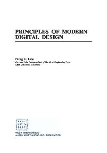
Figure 2.6 shows the amplitude ( H ( f ) lof the transfer function of the low-pass Butterworth filters for several values of their order n. It is seen that the curves of all orders pass through the 0.707 point at f = f,. As n + m, I H ( f ) Japproaches the ideal low-pass ('brickwall") characteristics:
IH(f)l =
{
1, I f l < f c 0, elsewhere.
It is left as an exercise for the reader to derive the conditions for which this system ex0 hibits a linear phase.
Example 2.3 An important family of linear systems is provided by the Butterworth filters. The transfer function of the nth-order low-pass Butterworth filter with cutoff frequency fc is 1 (2.28) H ( f )= D n ( j f / f c ) where
Dn(s)
fi
i=l
[s - e''n(Zi+n-1)/2n
1
(2.29)
2.2. Random processes 2.2.1. Discrete-time processes A discrete-time random process, or random sequence, is a sequence (&,) of real or complex random variables (RV) defined on some sample space. The index n is usually referred to as the discrete time. A discrete-time process is completely characterized by providing the joint cumulative distribution functions (cdf) of the N-tuples & + I , .. ., of RVs extracted from the sequence, for all
2. A mathematicaI introductiun
20
integers i and N , N > 0. If the process is complex, these joint distributions are the joint 2N-dimensional distributions of the real and imaginary components of &+I,. . . The simplest possible case occurs when the RVs in the sequence are independent and identically distributed (iid). In this case the joint cdf of any N-tuple of RVs factors into the product of individual marginal cdfs. For a real process,
.
N
,
Fci+l,ci+l,-.,t+N (xi+l r xi+2r ' ' ' xi+N)
xi+^)
=
(2.32)
j=1
where F e ( .) is the common cdf of the RVs. Thus, a sequence of iid RVs is completely characterized by the single function Fe(. ). A random sequence is called stationary if for every N the joint distribution does not depend on i. In other words, a stationary .. ., function of random sequence is one whose probabilistic properties do not depend on the time origin, so that for any given integer k the sequences (En) and (En+k)are identically distributed. An iid sequence extending from n = -m to +m is an example of a stationary sequence. The mean of a random sequence (En) is the sequence (En) of mean values
2.2.
Random processes
21
Markov chains For any real sequence
of independent RVs, we have, for every n,
where FCn1 c n - l , b - a , . . .(., ~. .) o denotes the conditional cdf of the random variable given all the "past" RVs . . ,to.Equation (2.35) reflects the fact that En is independent of the past of the sequence. A first-step generalization of (2.35) can be obtained by considering a situation in which, for any n,
En
that is, En depends on its past only through En-,. When (2.36) holds, is called a discrete-time (first-order)Markovprocess. If in addition every En can take only a finite number of possible values, say the integers 1, 2, . .. , q, then (En) is called a (finite)Markov chain, and the values of 5, are referred to as the states of the chain. To specify a Markov chain, it suffices to give, for all times n 0 and j , k = 1 , 2 , . . . , q, the probabilities P{En = j ) and P{En+l = k I En = j ) . The latter quantity is the probability that the process will move to state k at time n 1 given that it was in state j at time n. This probability is called the one-step transition probabili~firnctionof the Markov chain. A Markov chain is said to be homogeneous (or to have stationary transition probabilities) if the transition probabilities P{Ee+, = k I & = j ) depend only on the time difference m and not on C. We then call
>
+
The autocorrelation of
(5,) is the two-index sequence (T,,,)
such that
For a stationary sequence, (a) pn does not depend on n, and (b) T,,, depends only on the difference n sequence has a single index.
- m. Thus, the autocomelation
Conditions (a) and (b), which are necessary for the stationarity of the sequence (En),are generally not sufficient. If (a) and (b) hold true, we say that (En) is wide-sense (WS) stationary. Notice that wide-sense stationarity is exceedingly simpler to check for than stationarity. Thus, it is always expedient to verify whether wide-sense stationarity is enough to prove the properties that are needed. In practice, although stationarity is usually invoked, wide-sense stationarity is often sufficient.
the m-step transition probability function of the homogeneous Markov chain ((n)?=o. In other words, p$') is the conditional probability that the chain, being in state j at time C, will move to state k after m time instants. The one-step transition probabilities p$) are simply written pjk:
These transition probabilities can be arranged into a q x q transition matrix P : Pll
P12
p , P21
P22
.. ..
;;
[
'
Plq
'
P2q
..-
Pqq
1
22
2. A mathematical introduction
The elements of P satisfy the conditions
and
4
C p j k = l ri = 1 , 2 , ...,q k=l (i.e., the sum of the entries in each row of P equals 1). Any square matrix that satisfies conditions (2.40) and (2.41) is called a stochastic matrix or a Markov matrix. For a homogeneous Markov chain (&,)T=o,let denote the unconditional probability that state k occurs at time n; that is,
wF)
w$) = P{& = k),
k = 1 , 2 , . . . ,q
(2.42)
.. .w p ]
(2.43)
The row q-vector of probabilities wp), ,(4 = [wp) w p
is called the state distribution vector at time n. With w(O) denoting the initial state distribution vector, at time 1 we have
2.2.
Random processes
23
chain (&,)$=,is completely described by its initial state distribution vector w(O) and its transition probability matrix P . In fact, these are sufficient to evaluate P{&, = j) for every n 2 0 and j = 1 , 2 , . . . , q, which, in addition to the elements of P , characterize a Markov chain. Consider now the behavior of the state distribution vector w(")as n -t co.If the limit w = nlim + w w(") (2.49) exists, the vector w is called the stationary distribution vector. A homogeneous Markov chain such that w exists is called regular. It can be proved that a homogeneous Markov chain is regular if and only if all the eigenvalues of P with unit magnitude are identically 1. If, in addition, 1 is a simple eigenvalue of P (i.e., a simple root of the characteristic polynomial of P), then the Markov chain is said to befully regular. For a fully regular chain, the stationary state distribution vector is independent of the initial state distribution vector and can be evaluated by finding the unique solution of the system of homogeneous linear equations
subject to the constraints
Also, for a fully regular chain the limiting transition probability matrix or, in matrix notation,
w(l) = w(o)p
Similarly, we obtain
exists and has identical rows, each row being the stationary distribution vector w: rw1
and, iterating the process,
LwJ The existence of P Win the fo& (2.53) is a sufficient, as well as necessary, condition for a homogeneous Markov chain to be fully regular.
More generally, we have ,(e+m)
= ,(e)pm
Equation (2.48) shows that the elements of Pm are the m-step transition probabilities defined in (2.37). This proves in particular that a homogeneous Markov
Example 2.4 Consider a digital communication system transmitting the symbols 0 and 1. Each symbol passes through several blocks. At each block there is a probability 1 - p , p < 112, that the symbol at the output is equal to that at the input. Let to denote the symbol entering the first block and (,, n 2 1, the symbol at the output of the nth block
2.2.
2. A mathemalical introduction
24
Random processes
of the system. The sequence t o ,tl,t 2 , . . ., is then a homogeneous Markov chain with transition probability matrix
The n-step transition probability matrix is Figure 2.7: Generating a shift-register sequence.
The eigenvalues of P are 1 and 1 - 2p, so for p # 0 the chain is fully regular. its stationary distribution vector is w = [$ $1, and
I
i
I
Once the state set has been ordered according to the rule (2.55), each state can be represented by an integer number expressing its position in the ordered set. Thus, if z represents the state (a,,, a,,, . . . ,a,,) and j represents the state (a,, , a,,, . . . , a,,) the one-step transition probability p,, is given by
which shows that as n -t a symbol entering the system has the same probability 112 0 of being received correctly or incorrectly. where 6ij denotes the Kronecker symbol (bii = 1 and bij = 0 for i # j).
Shift-register state sequences An important special case of a Markov chain arises from the consideration of a stationary random sequence (a,) of independent random variables, each taking on values in the set {al, a 2 , . . . ,a M ) with probabilities pk = P{an = ak), k = 1,. . . , M , and of the sequence ( u , ) ~ =with ~,
If we consider an L-stage shift register fed with the sequence (a,) p i g . 2.7), a, represents the content (the "state") of the shift register at time n (i.e., when a, is present at its input). For this reason, (a,) is called a shifr-register stare sequence. Each a, can take on M L values, and it can be verified that (a,) forms a Markov chain. To derive its transition matrix, we shall first introduce a suitable ordering for the values of a,. This can be done in a natural way by first ordering the elements of the set {al, az, . . . ,a M ) (a simple way to do this is to stipulate that ai precedes a j if and only if i < j) and then inducing the following "lexicographical" order among the L-tuples aj, , a,, , . . . , aj,: (aj,, aj,, . . . , a,,) precedes (ail, a i l , . . . , ai,) jl < ill or jl = il and jz< i2, or ( jl = i l l jZ = i 2 , a n d j 3 < i 3 , etc.
Example 2.5 Assume M = 2, a1 = 0, a2 = 1, and L = 3. The shift register has eight states, whose lexicographically ordered set is
The transition probability matrix of the corresponding Markov chain is (000) (001) (010) (011) (100) (101) (110) (111) -p1 0 0 0 pz 0 0 0 P l o o o p z o o o 0 P 1 0 0 0 p 2 0 0 p= O P l O 0 o p z o 0 o o P l o o o p 2 o o o P l o o o p z O o O o p l o o o p ~ - 0 0 0 p1 0 0 0 pz
As one can see, from state (xyz) the shift register can move only to states (wxy), with probability pl if w = 0 and pz if w = 1. 0 Consider now the m-step transition probabilities. These are the elements of the matrix Pm.Since the shift register has L stages, its content after time n m,
+
2. A mathematical introduction
26
>
m L, is independent of its content at time n. Consequently, the states on+,, m 2 L, are independent of a,; so, f o r m 3 L,
2.2.
Random processes
27
(a) p(t) does not depend on time, and
t ~depends , only on the difference tl (b) ~ ( ( tz) write
- t 2 . Consequently, we can
%(ti - t2) 2 E[ 0,
Example 2.13 (continued) Assuming that the source symbols 0 and 1 are equally likely, we have
The probabilities appearing in (2.141) can be put in the form
As the source symbols are independent, we have Thus, w = [4
a a a], and
P{a,+e = ah, an+( = C j I a, = a k ,a, = z , ) = Ph P{an+e= C j I a, = a k , an = C,)
2. A rnathem&'cal introduction
50
for all k > 0. Thus
By combining together equations (2.141) to (2.144), we have
Gdf)=
I
Spectral analysis of deterministic and random signals
Observe that, from the equality p k P m = P m , we have
Fore = 0, we get instead
L
2.3.
L
C C p h p k s ; ( f ) ~ E k p e - ' s ;),l ( fe > 0
h=l k=l L
C P ~ S (; f )D4,( f ) , h=l
e=o
(2.145)
and, using definitions (2.135) to (2.140),
where the last equality holds because the matrix ( P k - P m )has all its eigenvalues with magnitude less than 1 (see Cariolaro and Tronca, 1974, for a proof). It is seen from (2.153) that the matrix A ( f ) , necessary to evaluate the RHS of (2.149), can be computed for each value of f by inverting a q x q matrix. This procedure is computationally inefficient because, if the spectrum value is needed for several f , many matrix inversions must be performed. For a more efficient technique, observe that A ( f ) is an analytic function of the matrix
Also, from (2.113) and the definition (2.139) of ~ ( f )we , get
or, equivalently, if (2.146) is used, so that A ( f )can be written in the form of a polynomial in A whose coefficients depend on f , say, In conclusion, the continuous and discrete parts of the power spectrum of our digital signal are given by The expansion (2.155) is not unique, unless we restrict K to take on its minimum possible value (i.e., the degree of the minimal polynomial of A ) . Here we assume that the reader is familiar with the basic results of matrix calculus, as summarized in Appendix B. In this situation, equating the RHS of (2.153) and (2.155). we get
and
K-1
C
where
m
~
(
f
2) ~ [ p e - -1 pm],-jz~fU
(2.151)
e=i Whenever there exists a finite N such that P N = Pm [e.g., when (a,) is a shift-register state sequence], A ( f ) involves a finite number of terms, and its computation is straightforward. If such an N does not exist, we need a technique to evaluate the RHS of (2.151).
[ e ' 2 " f T ~ - A ] P i ( f ) A i- I = O (2.156) i=O As the LHS of (2.156) is a polynomial in A having degree K , its coefficients must be proportional to those of the minimal polynomial of A . Denoting this minimal polynomial by
2. A mathematical introduction
52
and equating the coefficients of A,, i = 0,. . . , K, in (2.156) and in the identity
2.3.
Spectral analysis of deterministic and random signals
53
Example 2.12 (continued) We have
K
C 6 i ~=i 0
(2.158)
i=O
we get the coefficients /3,(f),i = 0,. . . , K - 1, needed to compute A ( f )according to (2.155). This procedure allows one to express A( f ) as a closed-form function o f f , which can be computed for each value of f with modest computational effort. Although the use of the minimal polynomial of A to obtain the representation (2.155) leads to the most economical way to compute the spectrum, every polynomial A(X) such that (2.158) holds can be used instead of the minimal polynomial. In particular, the use of the characteristic polynomial of A (which has degree q) leads to a relatively simple computational algorithm (due to Faddeev and first applied to this problem by Cariolaro and Tronca, 1974). According to this technique, A ( f )can be given the form
1
1 -1
1-11
Application of the Faddeev algorithm gives
and B3 = 0
Thus, using (2.149) and (2.159). we get where A(X)is now the characteristic polynomial of A, and B( . ) is a q x q matrix polynomial: B(X) = Xq-'Bo + X9-2B1 . . . -tBq-1 (2.160)
+
The polynomials B( . ) and A ( . ) can be computed simultaneously by using the following recursive algorithm (Gantmacher, 1959). Starting with 6, = 1 and Bo = I, let Example 2.13 (continued) From (2.149) we get
for k = 1 , 2 , . . . ,q. At the final step, B, must be equal to the null matrix, and 60 = 0, because the matrix A has a zero eigenvalue. Example 2.11 (continued) In this case P = Pw;thus, from (2.151) we have
so that
1 ~ S ( f ) l ~ ( l-cos2nfT) Sc(f) = ~ ( " ( f )= -2T
A special case We finally observe an important special case of the digital signal considered. If the modulator has only one state, or, equivalently, the waveform emitted at time nT depends, in a one-to-one way, only on the source symbol at the same instant, we have, from (2.149) and (2.150) and after some computations,
2. A mathematical introduction
2.4.
Narrowband signals and bandpass systems
and
f)}glare the Fourier transforms of the waveforms available from the
where {Si( modulator.
I-
Spectrum of z(t)
-----Spectrum of y(t)
2.4. Narrowband signals and bandpass systems When the signal x ( t ) is real, its Fourier transform X ( f ) shows certain symmetries around the zero frequency. In particular, the real part of X ( f ) is an even function of f , and its imaginary part is odd. As a consequence, to be in a POsition to reconstruct x ( t ) , it is sufficient to specify X ( f ) only for f >_ 0. NOW suppose that x ( t ) is passed through a linear, time-invariant system whose transfer function is the step function QU( f ) , Q a constant. At the output of this system ) be recovered without information loss. we observe a signal from which ~ ( tcan The impulse response of this system is
Figure 2.15: Spectra of a bareband signal z(t) and of a narrowband signal y(t).
+
Example 2-14 Let x(t) = cos(2nfot +4). Its Hilben transform is i ( t ) = sin(2nfot 4). so the corresponding analytic signal turns out to be d(t) = exp(j(2nfot 4)). We see from this simple example that the analytic signal representation is a generalization of the familiar complex representation of sinusoidal signals.
+
0
Among the properties of analytic signals, two are worth mentioning here. so its response to x ( t ) is ~ / . [2x ( t )+ jjc^(t)],where
(a) The operation transforming the real signal x ( t ) into the analytic signal
L(t) is linear and time invariant. In particular, if x ( t ) is a Gaussian random process, i ( t ) is a Gaussian random process. is called the Hilbert transform of x ( t ) . Notice that, because of the singularity in the integrand, the meaning of the RHS of (2.166) has to be made precise. Specifically, the integral is defined as the Cauchy principal value. The choice Q = 2 yields x(t)= %[d(t)] (2.167)
(b) Consider two real signals r ( t ) and y(t), and their product
where x ( t ) ,the system output, is
Assume that r ( t ) is a baseband signal. that is, its (amplitude or energy or power) spectrum is zero for 1f 1 > f l and y(t) is a narrowband signal, that is, its spectrum is nonzero only for f 2 < 1f 1 < f i , fr > f l (see Fig. 2.15). With these assumptions, from our definition of an analytic signal it follows that
Equation (2.167) shows that the original signal x ( t ) can be recovered from the output of a system with transfer function 2 u ( f ) by simply taking its real part. The complex signal d ( t )is called the analytic signal associated with x ( t ) .
that is, i ( t ) is the product of the real signal r ( t ) and the analytic signal associated with y(t).
2. A mathem&kd introduction
2.4.
Narrowband signals and bandpass systems
57
and a frequency fo E ( f , , f i ) , the analytic signal ?(t) can be written, according to the result of Example 2.15, in the form
q t ) = z(t)ei2"f0t (2.172) where Z(t)is a (generally complex) signal whose spectrum is zero for f > f2- fo and f < f 1 - fo (see Fig. 2.16 (b)). The signal Z(t)is called the complex envelope associated with the real signal x(t).From (2.172) we have the following representation for a narrowband x(t): x(t) = R[?(t)] = xc(t)cos 27r fot - xs(t)sin 27r fot
(2.173)
xC(t) 4 R[i-(t)]= R[?(t)e-jzrfot I = x(t)cos 27r fot + 2 ( t )sin 27r fot
(2.174)
where
and A
x d ( t ) = S[Z(t)]= S[i-(t)e-j2*fot I = -x(t) sin 27r fot 2 ( t )cos 27r fot
+
Figure 2.16: (a)Specrrum of a narrowband signal; (b)spectrum of irs compler envelope. (Figures nor ro scale.) Example 2.15 (Amplitude modulation of a sinusoidal carrier) Let y ( t )= cos 2?rfot, and let r (t) be a deterministic baseband signal whose Fourier transform Z(f ) is confined to the interval (- f l , fl), f l < fo. The analytic signal associated with their product is
;(t) = z(t)eJZrfot
(2.17 1)
(2.175) are baseband signals. Equation (2.173) and direct computation prove that xc(t) and x,(t) can be obtained from x(t) by using the circuitry shown in Fig. 2.17. There the filters are ideal low-pass. From (2.172) it is also possible to derive a vector representation of the narrowband signal x(t).To do this we define, at any time instant t , a two-dimensional vector whose components are the in-phase and quadrature components of Z(t), that is, xc(t)and x,(t) (see Fig. 2.18). The magnitude of this vector is
-4
A,(t)
IZ(t)j =
(2.176)
(see Fig. 2.19), and its phase is which shows that the amplitude spectrum of 5(t)is Z(f - fo),that is, it is obtained by translating the amplitude spectrum of z(t)around the frequency fo. 0
A
p,(t) = arg [Z(t)]= tan-'
+
2.4.1. Narrowband signals: Complex envelopes A narrowband signal is one whose spectrum is to a certain extent concentrated around a nonzero frequency. We define a real signal to be narrowband if its (amplitude or energy or power) spectrum is zero for ( f 1 $ (f l , f z ) , where ( f l ,f 2 ) is a finite frequency interval not including the origin (see Fig. 2.16 (a)). On the other hand, a signal whose spectrum is concentrated around the origin of the frequency axis is referred to as a baseband signal. For a given narrowband signal
x (t) xc ( t )
L
(2.177)
The time functions A,(t) and p,(t) 27rfot are called, respectively, the instantaneous envelope and the instantaneous phase of x ( t ) . The instantaneous frequency of x ( t ) is defined as 1/27r times the derivative of the instantaneous phase; that is,
where the primes denote time derivatives. From (2.173) to (2.177) the following representation of the narrowband signal x(t) can also be derived:
2.4.
2. A mathematical introduction
Narrowband signak and bandpass systems
qw
$ x, 0)
cos 2M0 t
sin 2M0 t Figure 2.19: Obtaining the instantaneous envelope of the narrowband signal x ( t ) .
Figure 2.17: Obtaining the real and imaginary parts of the complex envelope of the narrowband signal x ( t ) .
and v(t) = A&) m [ 2 x f o t
+ cp,(t)]
(2.183)
where
= 4t)
, I
X,
(t) IN-PHASE
Figure 2.18: Vector representation of the narrowband signal x ( t ) .
+ jv, (t)
(2.184)
is the complex envelope of v(t). The power spectrum of t ( t ) can be easily evaluated by observing that t ( t ) can be thought of as the output of a linear, time-invariant system with transfer function 2u( f ) whose input is v(t). Thus, its power spectrum equals the power spectrum of v(t) times the squared magnitude of the transfer function:
Equation (2.185) shows that the spectral density of t ( t ) is equal to four times the one-sided spectral density of v(t). Consider then the complex envelope G(t). From (2.184), its autocorrelation is
Narrowband random processes Consider now a real narrowband, WS stationary random process v(t), and the complex process t ( t ) v(t) + jD(t). (2.180)
and hence
The possible representations of v(t) are
I
v(t) = vc(t) cos 27r fot - v,(t) sin 27r fot
(2.182)
'&(f) = Gc(f + fo) (2.187) which shows that the power spectral density of the complex envelope G(t) is the version of G;(f) translated around the origin (see Fig. 2.20). Consider finally
2. A mathematical introduction
Narrowband signals and bandpass systems
2.4.
61
v,(t) and u,(t),the real and imaginary parts of the complex envelope. It can be shown (see Problem 2.20) that the following equalities hold:
where
Ru.uC( 7 ) i E[vS(t+ 7)uC(t)]
(2.191)
From (2.188) to (2.191) we can draw the following conclusions:
(a) As Ri(0) = EIfi(t)I2is a real quantity, Eqs. (2.190) and (2.191) show that E[v&)vc(t)I = 0 (2.192) That is, for any given t , u,(t) and v,(t) are uncorrelated RVs. As a special case, if u(t)is a Gaussian process, u,(t) and uc(t)are independent RVs for any given t . (b) From (2.185) and (2.186) it follows that Similarly, from (2.188), (2.190), and result (a) we have
~Ifi(t)I'= 2 E [ ~ , ( t = ) ]2E[uf(t)] ~
(2.194)
E[uC(t)l2 = ~ [ u f ( t= ) ]E[u2( t ) ]
(2.195)
Thus, That is, the average power of v,(t) and u,(t) equals that of the original process u(t).
u(t) is symmetric around the frequency fo, from (2.187) it follows that the power spectrum of fi(t) is an even function. This implies that Ri(r) is real for all T, SO (2.190) and (2.191) yield
(c) If the power spectrum of the process
E[u,(t + r)u,(t)]= 0 Figure 2.20: Representations of a ~ r r o w b a n dwhite noise process u ( t ) : ( a ) Power spectrum of u ( t ) ; (b)power spectrum of the analytic signal t ( t ) ;( c )power spectrum of the co.mplex envelope fi(t);( d )power spectra of the real and imaginary parts of f i ( t ) .
for all T
(2.196)
This means that the processes uc(t)and u,(t)are uncorrelated [or independent when u(t) is Gaussian]. Thus, in this situation,
2. A mathematical introduction
62
Example 2.16 Let x ( t ) be a bandpass real signal, and let Qz( f ) be the power density spectrum of its complex envelope. From (2.185)and (2.187)we have
Recalling the fact that Q,( f ) must be an even function o f f , the last equality yields
As an example, consider the signal
2.4.
Narrowband signals and bandpass systems
2.4.2. Bandpass systems The complex envelope representation of narrowband signals can be extended to the consideration of bandpass systems (i.e., systems whose response to any input signal is a narrowband signal). In the following we shall see how to characterize the effects of a bandpass system directly in terms of complex envelopes. In other words, assume that y(t) is the response of a bandpass system to the narrowband signal x(t). We want to characterize a system whose response to Z ( t ) , the complex envelope of x ( t ) ,is exactly tj(t),the complex envelope of y(t). Bandpass linear systems
where Elan]= 0 and E[a,,+,a;] = a~bo,,. From (2.122)-(2.124)we obtain the power spectrum of the complex envelope of x(t): 2
Q d f = $ls(f )I2. Hence, the power spectrum of the signal is
First, consider a bandpass linear, time-invariant system with impulse response h(t] and transfer function H ( f ) . The analytic signal representation aof h ( t ) is h ( t ) = h ( t ) j^h(t), which corresponds to the transfer function H ( f ) = 2H(f)u( f ) . If x ( t ) is the narrowband input signal and y(t) the response, the analytic signal $ ( t )can be obtained by passing x ( t ) into the cascade of the linear system under consideration and a filter with a transfer function 2u( f ) (see Fig. 2.21 (a)). In a cascade of linear transformations, the order of the operations can be reversed without altering the final result, so we can substitute the scheme of Fig. 2.21 (b) for that of Fig. 2.21 (a). Next, observe that i ( t ) has a Fourier transform equal to zero for f < 0. Hence, we can substitute a system with transfer function H ( f ) for another system having a transfer function H( f )u(f ) without alttring the output. The latter system (see Fig. 2.21 (c)) has an impulse response i h ( t ) ,input i ( t ) ,and output $ ( t ) . These signals are related by the convolution integral
+
Narrowband white noise As we shall see in later chapters, in problems concerning narrowband signals contaminated by additive noise it is usual to assume, as a model for the noise, a Gaussian process with a power density spectrum that is constant in a finite frequency interval and zero elsewhere. This occurs because a truly white noise would have an infinite power (which is physically meaningless), and because any mixture of signal plus noise is always observed at the output of a bandpass filter that is usually not wider than the band occupied by the signal. Thus, in practice, we can assume that the noise has a finite bandwidth, an assumption entailing no loss of accuracy if the noise has a bandwidth much wider than the filter's. A narrowband white noise is a real, zero-mean, stationary random process whose power density spectrum is constant over a finite frequency interval not including the origin. In Fig. 2.20 we showed the power spectrum of a narrowband white noise with a power spectral density No/2 in the band B centered at fo.
This equation becomes particularly useful if both i ( t ) and h ( t ) are expressed in terms of their complex envelopes. We get
which shows that $ ( t )is a narrowband signal, centered at fo, with complex envelope
In conclusion, the complex envelope of the response of a bandpass linear, timeinvariant system with impulse response h ( t ) to a given narrowband signal x ( t ) can be obtained by passing the complex envelope i ( t ) through the low-pass
2.4.
2. A mathematical introduction
Narrowband signals and bandpass systems
Figure 2.22: ( a ) Transferfunction of a bandpass linear system; ( b ) transfer&mction of a low-pars equivalent linear system. Figure 2.21: Three equivalent schemes to represent the analytic signal associated with the output of a linear system.
where
equivalent system whose impulse response is i k ( t ) ,or, equivalently, whose transfer function is H ( f + f o ) u ( f + f o ) (see Fig. 2.22). Notice that only if H ( f ) is symmetric around f o will the low-pass equivalent system have a real impulse response. A nonreal impulse response will induce in the output signal a shift of the phase and a correlation between the in-phase and quadrature components. These effects are usually undesired.
Example 2.17
is the "quality factor" of the circuit, and
Let s ( t ) = z(t)ei2rfot
where the Fqurier transform of z(t) is zero for If parallel resonator. Its transfer function is
1 > B, B < fo.
(2.201) Consider an LRC
-
I
If Q >> 1, the computation of h(t) becomes very easy. In fact, the second term in the RHS of (2.203) can be disregarded. Additionally, we can safely assume that the exponential factor exp {-nfotl2Q) is a bandlimited signal. Thus, from (2.203). we have 2Af0e-*fot/2~ $2rfot t 2 0, (2.204)
Q
where 1
fo = --t2 n m The corresponding impulse response is, f o r t
> 0,
In conclusion, h(q 2
Pnfo e - r f ~ t 1 2 ~ Q
7
t 2 o
2. A mathematical introduction
66
2.4.
Narrowband signals and bandpass systems
Notice that the approximations in the computation of i ( t ) make the Fourier transform 0 of (2.205) symmetric around the origin of the frequency axis.
.f
Bandpass memoryless nonlinear systems We shall now examine a class of nonlinear systems that are often encountered in radio-frequency transmission. We are especially interested in nonlinear timeinvariant systems whose input signal bandwidth is so narrow that the system's behavior is essentially frequency-independent. Moreover, the system is assumed to be bandpass. This in turn means that it can be thought of as being followed by a zonalfilter whose aim is to stop all the frequency components of the output not close to the center frequency of the input signal. For a simple example of such a system, consider a sinusoidal signal x ( t ) = A cos 277fot sent into a time-invariant nonlinear system. Its output includes a sum of several harmonics centered at frequencies 0, f o , 2f o , . . .. If only the harmonic at f o is retained at the output, the observed output signal is a sinusoid y ( t ) = F ( A )cos[277fot cp(A)].If we consider the complex envelopes 5 ( t ) = A and y ( t ) = F ( A ) exp[jcp(A)],we see that the system operation for sinusoidal inputs can be characterized by the two functions F( . ) and c p ( . ) . In the following we shall prove that this result holds true even when the input signal is a more general narrowband signal. Consider a narrowband signal x ( t ) , with a spectrum centered at f o . Its analytic signal representation can be given the form
Figure 2.23: Spectrum of the output of a memoryless nonlinear system whose input is a narrowband signal centered at frequency fo.
where
+
where A,(t) and cp,(t) are baseband signals. Letting
we rewrite (2.206) as q t ) = A,(t) e ~ * = ( ~ ) Consider then the effect of a nonlinear memoryless system whose input-output relationship is assumed to have the form
where S e [ . ] is an even function of $ , ( t ) , and S o [ . ] is an odd function. It is seen that y ( t ) , when expressed as a function of $,(t), is periodic with period 277. Thus, we can expand y ( t ) in a Fourier series:
The quantity c t ( A ) is generally complex. Its real and imaginary part are, respectively,
R[C!(A)]= and
$ [S.[Acos $1 cos $!. d$
1 8 [ c e ( A ) ]= i;;
1 2"
(2.212)
S,[A sin $1 sin C$ d$
From the definition (2.207) of & ( t ) , we see how (2.210) expresses the fact that the spectrum of y ( t ) includes several spectral components, each centered around the frequencies fCfo, e = 0 , 1,. . .. Figure 2.23 illustrates qualitatively this situation. Notice that we must assume that the signals c e [ A , ( t ) ]have spectra that do not significantly extend beyond the interval (- f o / 2 , f o / 2 ) . The assumption that the memoryless system is bandpass implies that only one of the spectral components of y ( t ) can survive at the system output (i.e., that centered at ff o ) . The analytic-signal representation of the output of such a bandpass memoryless system is then
where c(A)
A 2c1(A)
(2.215)
As c ( A ) is generally a complex number, we can put it in the form C ( A )= F(A)&*)
(2.216)
2. A mathematical introduction
2.5.
Discrete representdon of continuous signals
69
Example 2.18 (Polynomial-law devices) Consider a nonlinear system whose inputoutput relationship is y(t) = Czf(t) (2.220) t an integer greater than 1. 1f zit) is written in the form z(t) =
92[Z(t)ei2"jot]
= -1[ ~ ( t ) p l o t+ ~ * ( ~ ) ~ - j 2 " f o t 2 I
we get
d ( t )=
$ 6(:)
(2.221)
[ q t ) ] k [ ~ * ( ~ ) ] ~ - k $ 2 ~ ( 2 k - ~ ) j o t (2.222)
k=O
Figure 2.24: Representation of a bandpars memoryless nonlinear system.
or, in terms of complex envelopes,
When y ( t ) is filtered through a zonal filter, all its frequency components other than those centered at ffo will be removed. Thus, only the terms with 2k - t = f1 will contribute to the system output. This shows, in particular, that only when t is odd can the output of the zonal filter be nonzero. For t odd, the complex envelope of the system output is then
More generally, if the system is polynomial, i.e., L
~ ( t=) C a c z f ( t ) , i=l
Comparing the last equation with the complex envelope of the input signal,
f( t )= ~ , ( t ) & ~ ' ( ~ )
we shall get, for L odd,
(2.219)
we can see that the effect of a bandpass memoryless nonlinear system is to alter the amplitude and to shift the phase of the input signal according to a law that depends only on the values of its instantaneous envelope. This shows, in particular, that the system can be characterized by assigning the two functions F [ - 1 , c p [ . ] ,which describe the so-called AMIAM conversion and AMPM conversion effects of the system (AM denotes amplitude modulation and PM phase modulation). These functions can be determined experimentally by taking as an input signal a single sinusoid with a frequency close to fo and an envelope A, and by measuring, for different values of A, the output envelope F ( A ) and the output phase shift cp(A). Notice that, for the validity of this nonlinear system model, the functions F ( A ) and cp(A) should not depend appreciably on the frequency of the test sinusoid as it varies within the range of interest. Finally, notice that the system we are dealing with can be represented as in Fig. 2.24, where S, and So denote memoryless nonlinear devices. From this scheme it is seen that only if So is present can the system show an AMJPM conversion effect.
Notice that polynomial-law devices with real coefficients never exhibit M sion.
M conver0
2.5. Discrete representation of continuous signals In this section we consider the problem of associating a continuous signal with a discrete representation. In other words, we wish to represent a given continuous signal in terms of a (possibly finite) sequence. The representation may be exact or only approximate, in which case it will be chosen on the basis of acomprornise between accuracy and simplicity. As we shall see in later chapters, this representation makes it possible to impart a geometric interpretation to a signal set, and hence to visualize it by extracting from it the features that are relevant when the signals are used for modulation.
2. A mathematical introduction
70 2.5.1.
2.5. Discrete representation of continuous signals
Orthonormal expansions of finite-energy signals
A fundamental type of discrete representation is based on sets of signals called orthonormal. To define these sets, consider first the notion of the scalar pmduct between two finite-energy signals x ( t ) and y(t): it is denoted by ( x , Y )and defined as the value of the integral
If X ( f ) and Y ( f ) denote the Fourier transforms of x ( t ) and y ( t ) ,respectively, and we let ( X ,Y ) = X ( f ) Y * ( f df ) (2.227) -m
Parseval's equality relates the scalar products defined in the time and in the frequency domain: (2.228) ( x , Y ) = (x,y ) If ( x , y) = 0, or equivalently ( X , Y) = 0 , the signals x ( t ) and y ( t ) are called orthogonal. From the definitions of scalar product and of orthogonality, it immediately follows that ( x , X ) = EZ,the energy of x ( t ) ,and that the energy of the sum of two orthogonal signals equals the sum of their energies. Suppose now that we have a sequence ($i(t))iElof orthogonal signals; that is,
where I is a finite or countable index set. If Ei = 1 for all i E I, the signals of this sequence are called orthonormal. Obviously, an orthonormal sequence can be obtained from an orthogonal one by dividing each $;(t) by &. Given an orthonormal sequence, we wish to approximate a given finite-energy signal x ( t ) with a linear combination of signals belonging to this sequence, that is, with the signal
with respect to ci, i E I . By completing the square, we can also write
As the middle term in the RHS of (2.233) is nonnegative, Ee is minimized if the ci are chosen such as to render this term equal to zero. This is achieved for
ci = ( x , $i) =
/
m
-m
~ ( t ) $ : ( tdt, )
i
EI
(2.234)
The minimum value of &, is then given by
When c;, i E I, are computed using (2.234), the signal f( t ) of (2.230) is called the projection of x ( t ) onto the space spanned by the signals of the sequence ($i(t))iEl,that is, on the set of signals that can be expressed as linear combinations of the $;(t). This denomination stems from the fact that, if (2.234) holds, the error e ( t ) is orthogonal to every $i(t), i E I , and hence to f ( t ) . In fact,
(See Fig. 2.25 for a pictorial interpretation of this property in the case I = {1,2).) An important issue with this theory is the investigation of the conditions under which = 0. When this happens, the sequence ($Ji(t)),Er is said to be complete for the signal x ( t ) ,and from (2.235) we have the equality
A suitable criterion for the choice of the constants ci appearing in (2.230), and hence of the approximation f ( t ) ,is to minimize the energy of the error signal In this case we write
~ ( t=) Thus, the task is to minimize
C ci$i(t) iE1
although this equality is not to be interpreted in the sense that its RHS and LHS are equal for every t , but rather in the sense that the energy of their difference is
2. A mathematical introduction
2.5.
Discrete representation of continuous signals
73
Gram-Schmidt procedure Because of the importance of orthonormal signal sequences, algorithms for constructing these sequences are of interest. One such algorithm, which is computationally convenient because of its iterative nature, is called the Gram-Schmidt orthogonalizationprocedure. Let a sequence ( 4 i ( t ) ) C 1of finite-energy signals be given. We assume these signals to be linearly independent, i.e., to be such that any linear combination CEl c&(t) is zero almost everywhere only if all the q are zero. An orthonomal sequence ( $ ~ ~ ( t ) )is : , generated by using the following algorithm (see Problem 2.21). We first define the auxiliary signal $( ( t )equal to ( t ) :
Figure 2.25: P ( t ) is the projection of x ( t ) onto rk, the signal space spanned by $ l ( t ) and +2(t).
zero. This fact is often expressed by saying that the RHS and LHS of (2.237) are equal almost everywhere. In conclusion, once an orthonormal signal set has been chosen, a signal z ( t ) can be represented by the sequence ( c ~defined ) ~ by ~ (2.234). ~ This representation is exact (in the sense just specified) if the orthonormal set is complete with respect to z ( t ) .
then we normalize it to obtain the first orthonormal signal:
By subtracting from 42( t )its projection onto to ( t ) ,as shown in Fig. 2.26:
$ J ~
( t )we obtain a signal orthogonal
$ J ~
that we normalize to obtain the second orthonormal signal:
Example 2.19 (The complex Fourier series) The orthonormal sequence
By proceeding this way, we obtain the entire set of orthonormal signals. The general step of the algorithm is then: is complete for every complex signal x ( t ) defined in the interval (-T/2, T / 2 ) and having bounded variation with finitely many discontinuity points. The expansion
with
for i = 1,2,. . . , N (when i = 1 the sum in the first equality is empty).
Geometric representation of a set of signals is the familiar complex Fourier-series representation.
The theory of orthonormal expansions of finiteenergy signals shows that a signal z ( t ) can be represented by the (generally complex) sequence (ci)iE1of scalar
2. A mathematical introduction
Discrete representation of continuous signals
2.5.
where
75
a
j = l ,. . . ,N (2.244) or, equivalently, as a point in the N-dimensional Euclidean space whose coordinate axes correspond to the nonzero orthonomal signals found through the Gram-Schmidt procedure. In this situation, we say that the signal set {xi(t))iM_, has dirnensionali~N.
~ , j = ( x i , $ ~ ) i, = l , ..., M ,
Example 2.20 Consider the four signals
xi(t) = cos [ ~+t( 2
- l ) ~ / 2 ] t tE ( 0 , 2 ) , i = 1 , 2 , 3 , 4
(2.245)
Using the Gram-Schmidt procedure, we get $1
Figure 2.26: Generating a signal orthogonal to lCll ( t ) .
( t ) = cos 7rt
&(t) products (2.234). once an orthonomal sequence that is complete for x ( t ) has been provided. Now, if we consider a given sequence ( $ i ( t ) ) z l of N orthonormal real signals, it will be complete for any real x ( t ) that can be written as a linear combination of the $i ( t ) ,that is, in the f o m
= - sin nt
and
1Cl3(t) = 1Cl4(t) = 0 which shows that the signal set (2.245) has dimensionality 2 and is represented by the four vectors:
The reader should observe that the M-signal set
a
Thus, every such signal can be represented by the real N-vector x = ( x i , . . . ,X N ) , or, equivalently, by a point in the N-dimensional Euclidean space (i.e., the space of all real ordered N-tuples) whose coordinate axes correspond to the signals $ i ( t ) , i = 1 , . . . ,N . Consider now a set { x i ( t ) ) z l of real signals. Can we find an orthonomal sequence that is complete for these M signals? If so, we can represent x i ( t ) , x 2 ( t ) , . .. , x M ( t ) as M vectors or as M points in a Euclidean space of suitable dimensionality. If the signals in the set { x i ( t ) ) ~are , linearly independent, it suffices to apply to it the Gram-Schmidt procedure to find such an orthonomal sequence. In fact, (2.240) shows that each of the $ i ( t ) is expressed as a linear combination of signals in { x i ( t ) ) z l ;hence, each of the x , ( t ) can be expressed as a linear-combination of the $ i ( t ) . Suppose, instead, that only N signals in { x i ( t ) ) z l are linearly independent, and hence M - N of them can be expressed as linear combinations of the remaining signals. In this case, the Gram-Schmidt procedure can still be used, but it will produce only N < M nonzero orthonomal signals. Every x i ( t ) is then represented by the N-vector
x i ( t ) = cos[nt
+ 2(i - l)7r/M],
t tE (0, 2), i
=
1 , 2 , .. . , M
(2.246)
has dimensionality 2, and can also be represented using the same orthonomal basis.
Computing signal distances and scalar products Based on the procedure just developed, a real-signal set { x i ( t ) ) E l defined for 0 5 t < T can be represented by a set of vectors x , = ( x i l , . . . , X ~ N in ) the N dimensional Euclidean space. By using (2.242) and orthonormality of the signals $ i ( t ) , it can be easily proved that the following holds for any i = 1 , . . . , M :
which shows that the energy of a signal equals the squared length of the vector representing it. This equivalence between signal energy and distance of the vector from the origin is a very useful relation.
2. A mathematical introduction
2.5.
Discrete representation of continuous signals
77
This shows that the coefficients of the series expansion (2.252) are the samples of the signal z ( t ) taken at the time instants i/(2B),-co < i < co. Explicitly, from (2.250) and (2.253) we obtain
Moreover, we have
As two signals are orthogonal if their scalar product vanishes, we visualize orthogonal signals by two vectors perpendicular to each other. Finally,
The latter quantity is the (Euclidean) distance between signals zi(t),~ k ( t and ), is equal to the squared distance between the two vectors 4, xk.
Sampling expansion of bandlimited signals Consider now the set of signals x(t)strictly bandlimited in the frequency interval (-B, B), that is, such that their Fourier transform X ( f ) is identically zero for If 1 2 B. An orthonormal basis for any such z(t) can be found as follows. Expand X(f ) in a Fourier series according to (2.238) and (2.239). Then take the inverse Fourier transform to get an expansion for x(t).This procedure yields
and hence, by taking the inverse Fourier transform.
Equation (2.255) shows that every finite-energy signal with bandwidth B can be fully recovered from the knowledge of its samples taken at the rate of 2B samples per second. More generally, as any signal bandlimited in (-B, B ) is also bandlimited in (-B', B'),where B' > B, we can say that any finite-energy bandlimited signal can be represented by using the sequence of its samples, provided that they are taken at a rate not less than 2B. This minimum sampling rate of 2B is usually called the Nyquist sampling rate for z(t).If z(t)is a narrowband signal, it should be observed that it is convenient to apply the sampling expansion (2.255) to its complex envelope instead of the signal itself. This results in a much lower Nyquist frequency and, hence, in a more economical representation. Observe now that (2.255) can also be written in the form
Now, sin(2rBt)/(2rBt)can be interpreted as the impulse response of a linear, time-invariant system with frequency response and finally
=
m.
1=-m
sin 2rB[t- i/(2B)]
' %B[t - i/(BB)]
(2.252)
which is an expansion valid for every z ( t )with bandwidth B. Observing further that the integral in the RHS of (2.251) is proportional to the inverse Fourier transform of X ( f ) computed for t = i/(2B),ci can be put in the form
that is, an ideal low-pass filter with cutoff frequency B. Thus, (2.256) suggests how to implement a system that recovers z ( t ) from its samples. The sequence of samples is used to modulate linearly a train of impulses, which is then passed through an ideal low-pass filter (see Fig. 2.27). A frequency-domain interpretation of the reconstruction of a sampled signal can also be provided. Let the signal z(t) be sampled every T, seconds, and observe that we can write m
) a=-m
( -)
=( t )
E
1=-m
d(t - iT,)
(2.258)
2. A mathematical introduction
2.5. Discrete representation of continuous signals
Figure 2.27: Recovering a bandlimited signal x(t)from its samples. H ( f ) is an ideal low-pass filter with cutoff frequency B. The spectrum of this signal is obtained by taking the convolution of X ( f ) with the Fourier transform of a train of impulses with period T,. This is given by
[use (2.109)]. Thus, the spectrum of (2.258) is
which is periodic with period 1/T, (see Fig. 2.28). The original signal can be recovered from Xs(f) by using the ideal lowpass filter whose transfer function H ( f ) is shown in Fig. 2.28, provided that the translated copies of X ( f ) forming Xs( f ) do not overlap. This condition holds if 1 and only if B < - - B , that is, Ts fs
A
> 2B
(2.260)
where f, = 1/T, is the sampling rate. If (2.260) does not hold (i.e., the signal is sampled at a rate lower than Nyquist's), x(t) cannot be recovered exactly from its samples. The signal obtained at the output of the ideal low-pass filter has the Fourier transform
Figure 2.28: Sampling and reconstructing a bandlimited signal: frequency domain representation.
It is important to observe that if this situation occurs (i.e., the signal is "undersampled), even the phase of the sampling process affects the shape of the reconstructed signal. Specifically, if the sampled signal is
2.5.
&mete representalion of continuous signals
where 8 is a constant smaller than T,, at the output of the low-pass filter we get a signal whose Fourier transform is
If the bandwidth of x(t) does not exceed 1/ (2T,), then (2.262) gives the spectrum of x(t) (as it should). Otherwise, the shape of the signal recovered will also depend on the value of O. 2BT-theorem and the uncertainty principle The sampling expansion (2.255), which is valid for any x(t) bandlimited in the interval (-B, B), when applied to a signal vanishing outside the time interval (0,T) has nonzero terms occurring only for 0 il(2B) T (i.e., for 2 = 0,1,2, . . . ,2BT). Thus, any bandlimited and time limited x(t) is completely specified by 2BT 1 2BT constants. For real signals, this fact can be summarized by saying that "the space of real signals of duration T and bandwidth B has dimension 2BT." However, this argument is fallacious,because no bandlimited signal (besides the trivial null signal) can have a finite duration. The proof of this property is based on the fact that a signal x(t) whose amplitude spectrum vanishes for If 1 > B can be written as
+
-
H pO ~ fYIIHo(y I HO) and in So the remaining values. Values of Yl such that the integrand is zero do not affect the value of P(e), and hence may be included in either So or S1 arbitrarily. If we define the Iikelihood ratio between hypotheses Ho and Hl as A(Y) 2
and the decision rule becomes
< In PlPo -
choose Ho
if X(yl)
choose H1
if X(yl) > In 5 Pl
(2.291)
An important special case occurs when po = pl (i.e., the two hypotheses are equally likely). In such a case, the decision is made by comparing X(yl) against a zero threshold. Moreover, from (2.290) it is seen that the value of the constant No is not relevant to the decision. Hence, when po = pl the decision procedure does not depend on the spectral density of the noise. This simplification and the fact that the a priori probabilitiespo andpl might be unknown justify the frequent use of the simplified decision rule (called the marimum Iikelihood, or M L , rule):
the decision rule becomes
5 Pl
choose Ho choose H1
(2.292)
(2.286)
In conclusion, the optimum detector consists of a device that computes the likelihood ratio A(yl) and compares its value with the threshold po/pl. Explicitly, we have
so that, using (2.281),
0
although it gives minimum error probability only when po = pl. The rule (2.291) is referred to as the marimum a posterioriprobability, or MAP, rule. The structure of the ML detector is shown in Fig. 2.30. Example 2.22 (The integrate and-dump receiver) A simple special case of the general ML detector previously considered arises when the signal s ( t ) has a constant amplitude A in the interval 0 5 t < T . The task is then to decide between the two hypotheses
upon observation of y ( t ) for 0 have
5 t < T . In this case. E3 = A'T,
fib 1
Yl = -
T
Y(W
and from (2.281) we
(2.294)
2. A mathematical introduction
2.6.
Elements of detection theov
89
it is seen that, as P(e)is a monotone decreasing function of q, the error probability will decrease by increasing the level A, or by increasing the duration T of the observation interval, or by decreasing the noise spectral density. 0
Matched filter Figure 2.30: ML detection of a real signal s(t)in white Gaussian noise. Equation (2.294) shows that the sufficientstatistics for the detection are computed by averaging out the noise from the observed signal. This is obtained by integrating y(t) over the observation interval. Consider the performance of this detector when po = pl. The RV
is Gaussian, with mean zero and variance No/2. Thus, the error probability under Ho (i.e., the probability of choosing HI when Ho is true) is
P(e I Ho) = P{X(Yl)> 0 I Ho) = P {y > A f i / 2 )
where erfc ( .) is the complementary error function (see Appendix A). Similarly, the error probability under H1 is
so that
Consider again (2.281). This equation shows that the sufficient statistics can be obtained, apart from a constant factor, as the output at time t = T of a linear, time-invariant filter whose impulse response is
In fact, with this definition we have
A filter whose impulse response is (2.300),or, equivalently, whose transfer function is H ( f ) & s*(f)e-j2"fT (2.302)
A
where S ( f ) F [ s ( t ) ]is, called the filter matched to the s i g ~ s(t). l Thus, we can say that a matched filter whose output is sampled at t = T extracts from the observed signal y(t) the sufficient statistics for our decision problem. An important property of the matched filter is that it maximizes the signal-tonoise ratio at its output, in the following sense. When the filter input is the sum of the signal s(t)plus white noise v ( t ) ,at time t = T i t s output will be made up of two terms. The first is the signal part JTmH ( f ) S ( f ) e j 2 " fdf, T where H ( f )is the transfer function of the filter. The second is the noise part, a Gaussian RV with mean zero and variance (No/2)-/wm I H(f)I2d f . If we define the signal-to-noise ratio at the filter output
.
If we define the signal-to-noise ratio
(i.e., the ratio between the instantaneous power of the signal part and the variance of the noise part), we can show that C2 is maximized if H ( f ) has the form (2.302); that is, if the filter is matched to the signal s(t).The proof is based on Schwarz's inequality, which states that if A ( . ) and B( .) are two complex functions, then (2.304) IIAB'12 5 l IAI2 l PI2
,
2. A mathematical introduction
90
with equality if and only if A = aB', where a is any complex constant. Using (2.304) in (2.303), we get
2.6.
Elements of detection theory
91
j = 1 , 2 , . . . , M , on the basis of the observation of the values taken by the RVs Y l , Y z , . ... As the noise components V N + I , VN+Z,. .. ,are independent of ul, ..., V N ,and of the hypothesis, observation of Y N + ~YN+Z, . ... , does not add any information to the decision process. Thus, it can be based solely on the observaa [K, Yz,. . . , Y N ] , tion of K , Y z , .. . , YN.By defining the row N-vectors Y =
a a = [ul, 14,. . . , vN], and sj = [ s j l , sjz, . . . , s j N ] ,j = 1 , . . . , M , (2.310) can be reduced to the vector form Y
Thus, the maximum value of the signal-to-noise ratio C2 is obtained for Thus, the optimum detector sought for will operate as follows; Since a can be any constant, we can set a = 1 without loss of optimality, SO that the filter sought is indeed the matched filter as defined by (2.302). Notice that this filter may be physically unrealizable, in which case it is necessary to approximate it. Also, its response to the input s ( t ) is, at time t = T :
choose Hi if y E Si
(2.312)
where y denotes the observed value of the random vector Y, and S1, S2, .. . , SM is a partition of the N-dimensional vector space such that the rule (2.312) gives a minimum of the average error probability
that is, the energy of s ( t ) .
2.6.2. Optimum detector: M real signals in noise
a where pj = P { H i ) , j = 1 , 2 , . . . , M . It is seen from (2.313) that P ( e ) is minimized if every S j is chosen in such a way that
We now want to solve the most general problem stated at the beginning of this section, that is, to decide among the M hypotheses
upon observation of y ( t ) in the time interval ( 0 , T ) . The M real signals s j ( t ) , j = 1 , . . . , M , are known and have a finite duration and a finite energy. Us-
ing the Gram-Schmidt procedure, we can determine an orthonormal signal set {$i(t))El, N M , such that each s j ( t ) ,j = 1 , 2 , . . . , M , can be expressed as a linear combination of these signals. Also, consider a complete orthonormal signal sequence such that its first N signals are I l l ( t ) , ..., $ ~ ( t (see ) Problem 2.22). Denote with ( G i ( t ) ) z l this , sequence, and define
-d/2} = 1 - p Thus, 92 = (1 - 2p)(l - P ) Finally, 9, = P { - d l 2
Error probability of orthogonal signal sets. Another important signal configuration allows one to obtain an expression for P ( e ) which is nearly closed-form. This is the set of M orthogonal signals with equal energies, that is,
< nl < d / 2 ) P { - d / 2 < nz < d / 2 } = (1 - 2 ~ ) '
In conclusion, from the latter calculations and (4.40) we obtain
and hence
*. wi.
8
9 2 P ( e ) = 3p - -p 4 We observe here, also for later use, that for p > 1:
(a) Compute the capacity of the binary symmetric channel generated by this transmission scheme (see Section 3.3.2). *(b) Modify the receiver by introducing two thresholds at fA, so that an erasure is declared when the received signal component has an absolute value less than A. Derive the discrete equivalent binary erasure channel and compute its capacity as a function of A. Compare the two cases, and comment on them.
The average energy of this signal set is
(a) Show that the union bound (4.52) can be put in the form
4.7. ~ s s u m ae binary modulation scheme with signals, defined over (0, T),
C C erfc
l M
P(e) 5 -
8l(t) = 0, s2(t) = g s i n 2rrf2t,
f 2 = m/T,
and consider coherent and incoherent demodulation.
m an integer
djk
i=l jfi
*(b) Consider the four signal sets of Fig. 4.33 and compare their error probabilities by using the expression found in part (a).
4. Waveform transmission over the Gaussian channel
4.6.
Problems
Figure 4.33: Four octonary signal sets.
1:
Figure 4.32: Signal set of an octonary modulation scheme.
4.11. Define a configuration of biorthogonal signals as a set of M = 2 N signals in an N-dimensional signal space obtained by augmenting an original orthogonal signal set with the opposite -si of each signal s,. The case of N = 2 is shown in Fig. 4.34. Paralleling the calculations'that lead to (4.45). show that for biorthogonal signals
Figure 4.34: A biorthogonal signal set with M = 4. N = 2.
4.12. Given a set of M equally likely orthogonal signals of energy &, show that a signal set with the same error probability but minimum average energy can be obtained by translating its origin by 1,M
isfies the condition
These signals are said to be equally correlated.
a)gl
The resulting set of signals {si is called a simpler. Show that the simplex set has an average energy & ( l- l / M ) .
4.13. (Wozencraft and Jacobs, 1965) Assume that a set of M equal-energy signals sat-
(a) Prove that
4. Wavefonn transmission over the Gaussian channel
212
Hint: Consider
Izgl r.
4.6.
Problems (c) Show that (4.93) can be rewritten as
si
(b) Verify that the minimum value of p is achieved by a simplex set (see Prob-
lem 4.12).
P(e) = P{la12 > 1z1I2) = p{1t2l2 > Itl12) = P{R2
> R1)
Hint: Write lti12 = tfti.
(c) Prove that, for any p, the signal set has the same error probability as the simplex signal set with energy
Hint: Consider the set {si
- a)&,
with a = (1/M)
(d) Use the results of Appendix A to get
rglsi.
(d) Verify, as a consequence of part (c), that this signal set has the same error probability as an orthogonal signal set with energy
4.14. Prove (4.90X4.92).
(e) Finally, use the definitions of part (b) to show that in our case
4.16. Assume an M-ary modulation scheme with signals given by
4.15. This problem consists of a step-by-step derivation of (4.94). Define the two RVs
where 1
- IPI '
,m=-,
WP)
I PI
0
< t a. (a) Compute the exact value of the error probability for coherent demodulation. t(b) Determine the optimum values of a and b as a function of NO,the power spectral density of the noise. In particular, verify that as No -t 0 the minimum distance dmi, of the constellation is maximized, while for large No the best constellation has a -t 0. 4.18. By using (4.64) and an exponential approximation to the complementary error doubling the value of fi is equivfunction, prove that for P(e) values around
alent to losing about 0.2 dB in the ratio d i i , / ~ o . 4.19. Consider the binary transmission system based on the signal pair
where T < T. For a given value of fd, find the value of the correlation coefficient p that minimizes the error probability, and the corresponding value of P(e). 4.20. (*) Consider incoherent detection of M-ary orthogonal signals. Compare numer-
ically the resulting error probability with that of coherent detection, and observe the performance degradation due to the lack of knowledge of the carrier phase. By focusing on the binary case, observe how this degradation becomes monotonically smaller as the ratio & / N oincreases.
This chapter is devoted to the study of a number of important classes of digital modulation schemes. The concepts and the tools developed in Chapter 4 will be extensively used to analyze their performance. Transmission over the additive Gaussian noise channel is assumed throughout this chapter. The effect of other impairments other than Gaussian noise, viz., intersymbol interference and fading, will be examined in later chapters, while modulations aimed specifically at the wireless channel will be dealt with in Chapter 6. Here we aim at assessing how each modulation scheme uses the resources available, that is, power, bandwidth, and complexity, to achieve a preassigned performance quality as expressed in terms of error probability. Several constraints and theoretical limitations generate conflicts among the designer's desired goals. Therefore, the whole conceptual framework of this Chapter is finalized at clarifying the tradeoffs that are fundamental to the choice of a modulation scheme.
5.1. Bandwidth, power, error probability As in Chapter 4, we assume transmission over the additive white Gaussian noise (AWGN) channel with a two-sided noise power spectral density No/2. We denote by P the average power of the digital signal at the receiver front-end. As we assume for simplicity that the transmission channel introduces no attenuation, then P is also the average power of the signal observed at the transmitter output. In this section we define the parameters that will be useful to assess the performance of a digital modulation scheme, that is, bandwidth (and bandwidth efficiency), signal-to-noise ratio (and power efficiency), and error probability.
5. Digital modulation schemes
5.1.
Bandwidth, power, error probhility
217
The bandwidth of a real signal accounts only for the positive frequencies of its spectrum. Then we may use a number of different definitions:
(a) Null-to-null bandwidth. This measures the width of the main spectral lobe. It is simple to evaluate whenever the first two nulls around the carrier frequency enclose the main lobe, which in turn contains most of the signal power. (b) Fractional power-containment bandwidth. This is the frequency interval that contains (1 - c) of the signal power in positive frequencies (which is 50% of the total signal power). This definition is useful for wireless systems that share a common frequency band: for example, if a signal has 99.9% of its power in the bandwidth B allocated to it, then 0.1% of its power falls out of B, thus interfering with adjacent channels.
(c) Bounded power-spectral-density bandwidth. The criterion that specifies this bandwidth states that everywhere outside B the power spectral density does not exceed a certain threshold (for example, 50 dB below its maximum value). Figure 5.1: Powerdensiry spectnun of a PSK signal.
5.1.1.
Bandwidth
(d) Equivalent noise bandwidth. Originally defined for linear, time-invariant systems (see (2.89)), this measures the dispersion of the power spectral density around the carrier frequency.
where
The definitions above depend on the modulation scheme and on the specific signals used to implement it. Since in the following we shall be interested in a comparison among modulation schemes that leaves out of consideration the actual signals and focuses instead on the geometric features of the signal constellations, it is convenient to use an "abstract" definition of bandwidth. Let us recall from the 2BT-theorem of Chapter 2 that the dimensionality of a set of signals with duration T and bandwidth W is approximately N = 2WT. This motivates our definition of the "Shannon bandwidth" of a signal set with N dimensions as
The latter function, plotted in Fig. 5.1 on a logarithmic scale, is seen to consist of a main lobe surrounded by smaller sidelobes. Spectra of signals obtained at the output of different modulators have a similar appearance. If the spectrum had a finite support, i.e., it were nonzero only on a finite frequency interval, then it would be an easy matter to define the spectrum occupancy as the width of its support. However, for digital modulations employing finite-duration elementary waveforms (as is the case of the schemes described in Chapter 4). the power densities extend in frequency from -co to co,thus making it necessary to stipulate a conventional definition of bandwidth.
This bandwidth can of course be expressed in Hz, but it may be more appropriate in several instances to express it in dimensionsper second. The Shannon bandwidth is the minimum amount of bandwidth that the signal needs, in contrast to the definitions above. Any of them, which can be called Fourier bandwidths of the modulated signal, expresses the amount of bandwidth that the signal actually uses. In most cases, Shannon bandwidth and Fourier bandwidth differ little: however, there are examples of modulated signals ("spread-spectrum" signals) whose Fourier bandwidth is much larger than their Shannon bandwidth.
Consider first, for motivation's sake, an M-PSK signal whose elementary waveforms have duration T and amplitude A. The power density spectrum of such a signal is, as computed in Section 2.3,
5. Digital modulation schemes
5.1.
Bandwidth, power, error probability
219
ulator, M, and to the duration of these waveforms, T, by the equality
This is the rate in biVs that can be accepted by the modulator. The average power expended by the modulator is
p = -E T where E is the average energy of the modulator signals. Each signal carries log, M information bits. Thus, defining Eb as the average energy expended by the modulator to transmit one bit, so that E = Eb log, M , we have
We define the signal-to-noise ratio as the ratio between the average signal power and the average noise power. The latter equals (No/2).2W = NoW ,where now W is the equivalent noise bandwidth of the receiving filter, i.e., of the filter at the receiving front-end whose task, in our channel model, is to limit the noise power while leaving the signal undistorted. We have Figure 5.2: Power-containmentbandwidth of PSK and MSK. Example 5.1 (PSK) An M-PSK signal has 2 dimensions, so that W = 1/T. Its null-to-null bandwidth is 2/T, its equivalent noise bandwidth is 1/T, while its powercontainment bandwidth is plotted in Fig. 5.2. In the same figure the power-containment bandwidth of another modulation scheme, MSK, to be described in Chapter 6, is also 0 shown for future reference.
Note that in general, for any sensible definition of the bandwidth W , we have W = a / T , which reflects the fundamental fact from Fourier theory that the time duration of a signal is inversely proportional to its bandwidth occupancy. The actual value of CY depends on the definition of bandwidth and on the signals used by the modulator.
5.1.2. Signal-to-noise ratio In our discussion of Section 4.1 we have seen that the information rate of the 'source, R,, is related to the number of waveforms used by the memoryless mod-
Bandwidth efficiency and asymptotic power efficiency Expression (5.6)shows that the signal-to-noise ratio is the product of two quantities, viz., &b/No.the energy per bit divided by twice the power spectral density, and R,/W, the bandwidth (or spectral) efficiency of a modulation scheme. In fact the latter, measured in biVs/Hz, tells us how many bits per second are transmitted in a given bandwidth W . For example, if a system transmits data at a rate of 9,600 biVs in a 4,800 Hz-wide system, then its spectral efficiency is R, = 2 biVs/Hz. The higher the bandwidth efficiency, the more efficient the use of the available bandwidth made by the modulation scheme. We also observe that if W denotes the Shannon bandwidth then R,/ W may also be measured in biVdimension. We have
Since two-dimensional modulation schemes are especially important in applications, often the spectral efficiency is measured in bits per dimension pair. We now define the asymptotic power efficiency y of a modulation scheme as follows. From (4.65) we know that for high signal-to-noise ratios the error
5, Digital modulation schemes
220
probability is approximated by a complementary error function whose argument is d ~ . / 2 f i .Define 7 as the quantity satisfying
5.2.
7 = -&in
(5.8)
4Eb In words, 7 expresses how efficiently a modulation scheme makes use of the available signal energy to generate a given minimum distance. Thus we may say that, at least for high signal-to-noise ratios, a modulation scheme is better than another (having a comparable average number of nearest neighbors 0)if its asymptotic power efficiency is greater. For example, the antipodal binary modulation of Chapter 4 has f i = 4 and d ~ =, 2 f i , so that 7 = 1, This may serve as a baseline figure. 5.13.
Error probability
Most of the calculations in Chapter 4 were based on symbol error probability. TO allow comparisons among modulation schemes with different values of M , and hence whose signals carry different numbers of bits, a better performance measure is the bit e m r probability Pb(e),often also referred to as bit-emr rate (BER).This is the probability that a bit emitted by the source will be received erroneously by the user. In general, it can be said that the calculation of P ( e ) is a far simpler task than the calculation of Pb(e). Moreover, the latter depends also on the mapping of the source bits onto the signals in the modulator's constellation. A simple bound on Pb(e)can be derived by observing that, since each signal carries log2 M bits, one symbol error produces at least one bit error and at most log, M bit errors. Therefore.
Since (5.9) is valid in general, we should try to keep Pb(e)as close as possible to its lower bound. One way of achieving this goal is to choose the mapping in such a way that, whenever a symbol error occurs, the signal erroneously chosen by the demodulator differs from the transmitted one by the least number of bits. Since for high signal-to-noise ratios we may expect that errors occur by mistaking a signal for one of its nearest neighbors, then a reasonable pick is a mapping such that neighboring signal points correspond to binary sequences that differ in only one digit. When this is achieved we say that the signals are Gray-mapped, and we
22 1
approximate Pb(e) by its lower bound in (5.9). In the following we shall provide examples of Gray-mapped signal constellations, but we hasten to observe here that exact Gray-mapping is not possible for every conceivable constellation. 5.1.4.
that is,
Pulse-amplitude modulation (PAM)
'Itade-offs in the selection of a modulation scheme
In summary, the evaluation of a modulation scheme may be based on the following three parameters: the bit error probability Pb(e),the signal-to-noise ratio EbINo necessary to achieve Pb(e),and the bandwidth efficiency RJW. The first tells us about the reliability of the transmission, the second measures the efficiency in power expenditure, and the third measures how efficiently the modulation scheme makes use of the bandwidth. For low error probabilities, we may simply consider the asymptotic power efficiency 7 and the bandwidth efficiency. The ideal system achieves a small Pb(e)with a low Eb/Noand a high RJW: now, Shannon's theory as discussed in Chapter 3 places bounds on the values of these parameters that can be achieved by any modulation scheme. In addition, complexity considerations force us to move further apart from the theoretical limits. Consequently, complexity should also be introduced among the pararneters that force the trade-off in the selection of a modulation scheme.
5.2.
Pulse-amplitude modulation (PAM)
This is a linear modulation scheme, also referred to as amplitude-shift keying (ASK). A sequence $, of K source symbols is carried by the signal
where the RVs tktake on values in the set of equally-spaced amplitudes {ai)& given by d ai=(2i-1-M)-, z = l , 2 ,...,M (5.1 1) 2 Consequently, the waveforms used by the modulator are a set of scalar multiples of a single waveform: { s i ( t ) } E 1= { a i } E 1 s ( t ) .If ~ ( tis) a unit-energy pulse, it plays the role of a basis signal in an orthonormal expansion, which shows that this signal set is one-dimensional. The geometrical representation of PAM signal sets for d = 2, M = 4 and M = 8, is shown in Fig. 5.3, where the signals are Gray-mapped. The simplest form of optimum demodulator has only one correlator,or matched filter (with impulse response s(T - t ) ) .Its output is sampled, then compared to a
5. Digital modulation schemes
5.2.
Pulse-amplitude modulation (PAM)
Figure 5.3: Geomerrical represenrarion of Gray-mapped PAM signal sers. set of M - 1 thresholds, located at the midpoints of adjacent signal points. Theresult of these comparisons provides the minimum-distance (and hence maximumlikelihood) decision.
5.2.1. Error probability The symbol error probability of PAM with coherent demodulation can be evaluated as shown in Section 4.2.3. Explicitly, we have the probability of a correct decision 1 ( M - 2161 p(c) = [%I
Figure 5.4: Symbol error probabililies of M-ary PAM. Here vb = Eb/N0.
To express P ( e ) as a function of &/NO,observe that the average signal energy is, from (5.11).
M
where ql is the correct-decision probability for the two outer points of the constellation, and q2 is the same probability for the ( M - 2 ) inner points. By defining
we have ql = 1 - p and 92 = 1 - 2p, so that
Thus
The error probabilities for several values of M are plotted in Fig. 5.4. The asymptotic power efficiency is the factor multiplying &/No in the argument of erfc(. ). For this scheme we have
3 log, M TPAM = M2 - 1 and finally
,
which can be seen to decrease when M increases. In PAM the average energy of the transmitted signal differs from the peak energy Ep. which is the energy of the maximum-amplitude signal. When design
5. Digital modulation schemes
224
constraints are put on the peak transmitted power, we may want to express P ( e ) in terms of E, = ( M - 1),&/4. From (5.12) we obtain
5.3.
Phase-shifC keying (PSK)
225
T , so that the envelope of a PSK signal is constant (but other waveforms are possible). We can write explicitly
k=O = I ( t ) cos 27r fot
For example, for M = 4 we find that E, is 2.55 dB larger than E.
5.2.2.
Power spectrum and bandwidth efficiency
- Q ( t )sin 27r fot
(5.20)
where we have defined the in-phase and quadrature components of the PSK signal:
The power spectral density of the PAM signal is obtained from (2.125) as A
Q(t) = A where S ( f ) is the Fourier transform of s(t). Notice that here and in the following, when dealing with power spectral densities, we extend the summation in (5.10) from -oo to oo,so as to avoid edge effects and render the signal widesense cyclostationary. The Shannon bandwidth of this modulation scheme is W = 1/2T, so that its bandwidth efficiency is = 2 log, M
($1
-
sin 4ku ~ (-t k T )
The PSK signal set is represented geometrically in Fig. 5.5 for M = 2, M = 4, and M = 8. In all cases the signals are Gray-mapped. We have seen in Example 2.20 that the PSK signal set is two-dimensional. The modulators of 2-PSK and 4-PSK are shown in Figs. 5.6 and 5.7.
5.3.1.
Error probability
PAM
This increases with M . In conclusion, for PAM, increasing M improves bandwidth efficiency but decreases power efficiency.
5.3.
x
~~
Phase-shift keying (PSK)
This is a linear modulation scheme in which the source symbols shift the phase of a camer signal. A sequence of K symbols is represented by the signal
Consider coherent demodulation of PSK. For illustration purposes, the structure of the demodulator of 4-PSK is shown in Fig. 5.8.
Binary PSK The exact error probability of binary PSK is determined by observing that 2PSK is an antipodal modulation scheme. Hence, by using the result (4.37), and observing that for a binary scheme Eb = E, we obtain
Quaternary PSK where Ck = $
4 and ~ ~ each
discrete phase q5k takes values in the set
with a an arbitrary constant phase. In the following the modulator waveform s ( t ) is assumed to be u T ( t ) , a rectangular pulse of amplitude A and duration
The error probability of quaternary PSK (CPSK, or QPSK) was determined explicitly in Subsection 4.2.3. By observing that now Eb = E/2 and dmi, = = 2Eb,from (4.39)-(4.40) we have
a
5. Digital modulation schemes
5.4.
Quadrature amplitude modulation (QAM)
Source
Modulated
LEVEL
symbols GENERATOR
signal
*
GENERATOR
Figure 5.6: Binary PSK modulator.
5.3.2. Power spectrum and bandwidth efficiency The power spectral density of the PSK signal is expressed by (5.1)-(5.2). Since N = 2, the Shannon bandwidth of this modulation scheme is W = 1/T, so that its bandwidth efficiency is f 1,
Figure 5.5: Geometrical representation of Gray-rnapped PSK signal sets.
( )
M-ary PSK For general M-ary PSK we may use the upper and lower bound to P ( e ) derived in Subsection 4.3.1. Here Eb = E l log, M , and from (4.49) we have
PSK
= log, M
(5.25)
This increases with M. In conclusion, for PSK (as for PAM) increasing M improves bandwidth efficiency but decreases power efficiency.
5.4. Quadrature amplitude modulation (QAM) (Ji
The err& probabilities for several values of M are plotted in Fig. 5.9. The asymptotic power efficiency of PSK is given by 7r
yps, = sinZ- . log, M M -,
which can be seen to decrease as M increases, M > 2. (Notice how for both M = 2 and M = 4 we have y = 1).
This is a linear modulation scheme such that the source symbols determine the amplitude as well as the phase of a carrier signal. Contrary to PSK, the signal envelope is not constant. A sequence of K symbols is represented by the signal
5. Digital modulation schemes
4
WEL GENERATOR
5.4.
Quadrature amplitude modulation (QAM)
wTO SERIAL
CONVERTER
Source symbols
W0PHASE
Figure 5.8: Quaternary PSK demodulator 1
0
0
1
1
1
1
0
1
1
t
t
which expresses the transmitted signal in the form of a pair of orthogonal carriers modulated by a set of discrete amplitudes. This family of signal constellations is two-dimensional, and its modulator and demodulator have the same structure of those of PSK. Several QAM families may be selected. Fig. 5.10 shows two constellations with M = 8 and M = 16. These are obtained by choosing a set of discrete amplitude levels (in number of 2 and 4, respectively), and four equally-spaced phase values in each. Another choice, way more popular, consists of picking an infinite grid of regularly spaced points, with coordinates (nl 1/2, n2 1/2), nl and n2 two relative integers (that is, n1 E Z and n2 E Z), and carving out of it a finite constellation with M points (for example, under the constraint that the average energy be minimized). This infinite grid can be thought of as generated by translating the so-called square lanice Z2 with points ( n l , nz), nl and n2 any two relative integers. This lattice, as well as its translated version, has minimum distance 1. Three square constellations obtained from the translated lattice Z2 + $) with M = 4, M = 16, and M = 64 are shown in Fig. 5.11. When M is not a power of 4, the corresponding constellation is not square, and can be given the shape of a cross to reduce its minimum average energy. Two examples of these "cross constellations" are shown in Fig. 5.12 for M = 32 and M = 128. Another constellation can be obtained by picking signal points from the lattice D2. This is derived from Z2 by removing one out of two points in a checker-
+
Figure 5.7: Quote-
PSK modulator
where the discrete RV Jk is defined as Jk
(i,
2 JL + jJl = A&@L
and s ( t ) is a baseband complex signal with duration T. When the latter is a rectangular pulse of unit amplitude, i.e., s ( t ) = u ~ ( t we ) , can rewrite (5.26) as K-1
q ( t )=
k=O
{JLcos 2sfot - J[ sin 2sfot) uT(t - kT)
(5.27)
+
5. Digital modulation schemes
5.4.
Quadrature amplitude modulation (QAM)
Figure 5.10: Two QAM constellations with M = 8 and M = 16.
Figure 5.9: Symbol error probabilities of PSK. Here 17b = Eb/No. board fashion, so that the minimum distance among the remaining points is maximized. In formulas, Dzis the set of the integer pairs (nl,n2)with even sum nl nz. The lattice Dz, whose minimum distance is and an 8-point constel6) are shown in Figs. 5.13 and 5.14,respectively. lation carved from Dz+
+
a,
(6,
5.4.1. Error probability
+
Square constellations carved from ZZ (i,$) The symbol error probability of M-points square constellations carved from ZZ (i,i) can be easily derived from the observation that they consist of the cross-product of two independent PAM constellations with signals each and an average energy one half that of the QAM constellation (so that &b is the same for both constellations). To see this, note that a square constellation can be demodulated independently on the two coordinate axes, corresponding to the in-phase and quadrature components. Thus, the probability of correct detection in this M-signal QAM equals the 'square of the probability of a correct detection for a PAM constellation with
+
Figure 5.11: Three square Q A M constellations carvedfrom the translated lattice Z
+
1 1 (z, 5).
signals obtained by projecting the former on one coordinate axis. If p denotes the symbol error probability in each PAM constellation, we have
5. Digital modulation schemes
5.4.
Quadrature amplitude modulation (QAM)
+ (i,i).
Figure 5.14: An 8-point signal constellation carvedfiom D2
large M and large Eb/No)can be obtained by writing P(e) < 2 p and observing that (1 - I/-) < 1 in (5.28X5.29). Equivalently,we may observe again that a square constellation can be thought of as the product of two PAM with signals and half the energy. By using (5.12) we obtain
a
Figure 5.12: Two cross constellations c a r v e d f i m the translated lanice Z
+ (i,4). Moreover, the average number of nearest neighbors is approximately 4 (it is lower for the outer points of the constellation, and exactly 4 for all inner points). Thus, from (4.64) we have
Cross constellations carved from Z2+ ( f , f ) Figure 5.13: The lattice D2, obtained from the square lattice by removing every second point in a checkerboard fashion.
where, from (5.13) with M changed into a
,
' A simple upper bound to P(e) (which is also an approximation useful for
To construct a cross constellation with M = 25+2a signals we may use the 32square template of Fig. 5.15. We scale it, by partitioning each square into four squares, p times. The cross constellation is then the set of 25+2a points from Z2+ (f , f ) located in the middle of the resulting squares. For the error probability of cross constellations no exact result is available. However, for large enough M the approximation (5.30) still holds. In fact, the average number of nearest neighbors is still about 4, while the average energy is slightly lower than for square constellations. To justify the latter statement, we
5. Digital modulation schemes
5.4.
Quadrature amplitude modulation (QAM)
Figure 5.15: Template for a 32-point QAM cross constellation. observe that for large M the average energy of the constellation, that is,
can be thought of as the discrete approximation to the integral
where the integration is performed over the domain that encloses the constellation. For example, if it is performed over the square with side a d m i . (and hence area Md;,) that encloses the square constellation with M points, it yields the approximation E = Mdki,/6. For the cross constellation described above, we obtain & w 31/32. Mdkin/6, a good approximation even for moderate values while of M . For example, M = 128 yields the approximate value 20.67 d:,, the true value obtained from direct computation is & = 20.5 diin. We conclude that the average energy of a cross constellation is lower than that of a square constellation by a factor 31/32, i.e., 0.14 dB. The-error probabilities for square constellations with several values of M are plotted in Fig. 5.16.
Figure 5.16: Symbol error probabilities of square constellations carved from Z 2 1 1 (?, ?). Here q b = &/NO.
+
which can be seen to decrease when M increases. It is instructive to compare the asymptotic power efficiencies of PSK and QAM. We expect the latter to be larger, since QAM does not suffer from the constraint of having all its signal points on a circumference for constant envelope. By taking the ratio between (5.32) and (5.24) we obtain
For large M , this ratio approaches
5.4.2. Asymptotic power efficiency From (5.30) the asymptotic power efficiency of QAM is given by
, YQAM
=
3 log, M
5
and hence increases linearly with M. For example, for M = 64 the ratio between the two efficiencies is close to 10 dB, and for M = 256 is close to 15.9 dB.
5. Digital modulation schemes
236
5.4.
Quadrature amplitude modulation (QAM)
5.43. Power spectrum and bandwidth efficiency The power spectral density of the QAM signal is given by (5.1), where now
and S(f ) is the Fourier transform of the complex signal S ( t ) . Since N = 2, the Shannon bandwidth of this modulation scheme is W = 1/T, so that its bandwidth efficiency is the same as for PSK:
As for PAM and PSK, this increases with M . In conclusion, for QAM, increasing M improves bandwidth efficiency but decreases power efficiency. 0
5.4.4. Q A M and the capacity of the two-dimensional channel We have seen that, in the absence of a constant-energy constraint, QAM is more efficient than PSK. In this section we shall examine how this modulation scheme compares with the limiting performance predicted by information theory. Recall from Chapter 3 the expression of the capacity of the additive white Gaussian noise (AWGN) channel, expressed in bitIslHz:
2
4
6 8 normalized SNR (dB)
10
Figure 5.17: Symbol errorprobability vs. normalized SNRfor QAM. The Shannon limit is also shown
This expression of error probability can be compared with the Shannon capacity bound derived from (5.35). This states that for large SNR there exists a coding/ modulation scheme which achieves, over the AWGN channel, arbitrarily low error probabilities provided that
By recalling (5.34) we may write Eb SNR = log2 M -
No
Let us define the normalized SNR as SNRo = SNR 2-
(5.36)
where r2 denotes the transmission rate in bits per dimension pair. Now, consider QAM with M = 2'2 equally likely signals. Its symbol error probability over the AWGN channel is given by (5.30), which can be rewritten, for large M, in the form 4
e
a 2e c
(
)
=2e c
(
)
(5.37)
This implies that arbitrarily low error probabilities can be achieved for any normalized SNRo > 1 (i.e., 0 dB). Fig. 5.17 compares the symbol error probability achieved by QAM with the Shannon bound. From this figure we may observe that for an error rate of the order of there is a SNR gap of about 6 dB, which becomes 7.5 dB at and about 9 dB at lo-'. As we shall see later, most of this gap can be filled by a combination of coded modulation and shaping.
5. Digital modulation schemes
238
Orthogonal frequency-shift keying (FSK)
5.5.
5.5. Orthogonal frequency-shift keying (FSK) This is a nonlinear modulation scheme such that the source symbols determine the frequency of a constant-envelope carrier. Specifically, it is assumed that the modulator consists of a set of M separate oscillators tuned to the desired frequencies.' A sequence of K symbols is represented by the signal
where the discrete RV & takes values in the set (22 - 1- MI&, is the separation between adjacent frequencies. The transmitter uses the signals
and hence 2fd
They have common energy E = A 2 T / 2 , and a constant envelope. By choosing appropriately the frequency separation, the signals can be made orthogonal. Specifically, we have
/n s i ( t )y ( t )dt T
= A'
/
0
T
cos 2 r f i t . cos 2 n f j t dt
sin 4n(z - j)fdT ++f j ) T +-A2T 2 4 ~ (-i j ) fdT
Figure 5.18: Symbol error probability of orrhogonal FSK. Here rp, = Eb/NO.
5.5.1.
Error probabiIity
By bounding the symbol error probability with the union bound of Example 4.5, we obtain
- A2T sin 2 ~f i ( f j ) T
2
2T(fi
We assume that the product foT of carrier frequency and symbol interval is so large that the first term in the last expression can be disregarded. Thus, the scalar product of two distinct waveforms is zero whenever 4n fdT is a nonzero multiple of T . The minimum frequency separation yielding orthogonal signals is
'Another practical possibility is the use of a single oscillator whose frequency is modulated by source bits. The resulting FSK signal is phase-continuous, and the absence of abrupt phase fransitions yields a narrower power density spectrum. See Chapter 6 for further details.
(See Fig. 5.18). For this modulation scheme the bit error probability can be easily related to P ( e ) . Choose a position in the (log, M)-tuple of bits associated with any signal. Then M / 2 signals have a 0 there, and M / 2 have a 1 . We have an error in that position if the demodulator selects one out of the M / 2 signals with the wrong bit there. Now, when the demodulator makes an error, all the M - 1 incorrect signals have the same probability of being selected, because all are at the same distance dmi, from the transmitted signal and the noise is spherically symmetric. In conclusion,
5.5.
5. Digital modulation schemes
Orthogodfrequency-shifC keying (FSK)
55.2. Asymptotic power efficiency From (5.43) the asymptotic power efficiency of orthogonal FSK is given by TFSK
=
1
log2 M
(5.44)
and increases with M.
55.3. Power spectrum and bandwidth efficiency By using eqs. (2.164) and (2.165) under the assumption that all signals are equally likely to be transmitted, we obtain the power density spectrum of the FSK signal as
and I I,.
where as usual Si(f) denotes the Fourier transform of signal s i ( t ) , i = 1,.. . , M . Example 5.2
Figure 5.19: Power density spectrum of binaiy FSK (continuous part).
Consider binary FSK signaling, with
sl ( t ) = A cos 2a(fo- fd)t
and
s2(t)= A cos 2a(fo
./I,
+ fd)t
The corresponding complex envelopes are Sl(t) = ~e-j2"fdt
and
S2(t)= ~
2
~
~
+fd)
~
~ Finally, the power spectrum of the real signal can be obtained from
and their Fourier transforms are S l ( f ) = g(f
f
and
S 2 ( f )= g(f - f d )
where g ( f ) is the &insform of the rectangular pulse A u ~ ( t ) :
The power density spectrum of the complex envelope of the modulated signal is given by
a
A ( f )= { d C )-( ffo ) + @ ( - f
- f o ) d d ) ( f - f o ) + dd)(-f -lo)}
Curves showing the continuous part of the spectrum of FSK for some values of 2fdT can be found in Fig. 5.19. Table 5.1 lists the amplitudes of the line spectrum for the same values of 2fdT. 0
'.,,r,l(
#Y'
In interpreting the results described above for the power density spectrum of FSK, one should keep in mind that they were obtained under the fundamental assumption, made in this chapter, that the modulation scheme is memoryless. This
#,.d*,
..*"*
5. Digital modulation schemes
5.6.
Multidimensional signal constellations: Lam'ces
243
R. One then derives the properties of S from the properties of A and those of R. We start by listing some parameters useful for assessing the quality of a multidimensional constellation. Bit rate and minimum distance. Let S denote an N-dimensional signal constellation, (Stthe number of its points, and q(x) the probability of transmitting the signal x E S . Its bit rate is the number of bits per dimension carried by each signal, that is, log2 J S ( / N . Its normalized bit rate is the number of bits carried per dimension pair: Table 5.1: Discrete power densiry spectrum for the signals of Example 5.2: Coefficients of the line components in dB.
implies, as briefly mentioned at the beginning of this section, that the pulses at different frequencies be generated independently: in particular, no phase depen.dence among them is assumed. This model fits a situation in which the modulated signal is obtained by switching at a rate 1 / T among M different oscillators that generate signals with the same initial phase in each symbol interval. This may occur when the signal waveforms are generated digitally.
The normalized minimum distance of the constellation S is the ratio between dki, and the average signal energy E , where
Figure of merit. The constellationjgure of merit of S is the ratio between d k i , and the average energy of S per dimension pair:
Bandwidth efficiency. Here N = M , so that the Shannon bandwidth of this modulation scheme is W = M/2T, and its bandwidth efficiency is
We note that, unlike with PAM, PSK, and QAM, by increasing M the bandwidth efficiency of orthogonal FSK decreases. On the other hand, its power efficiency increases.
The constituent constellation. Assume the N-dimensional constellation to be generated by transmitting N/v consecutive v-dimensional elementary signals (in typical wireline modems v = 2, with QAM as elementary signals). If the projections of S onto coordinate pairs (1,2), (3,4), .. . , ( N - 1,N ) are identical, we call this common constellation the constituent 2 - 0 constellation of S. This is denoted by S2, and the induced probability distribution by q2( . ). We desire that the size (Sz(be as small as possible. With this definition of S2we have
5.6. Multidimensional signal constellations: Lattices In this section we focus our attention on a special case of multidimensional signals, those generated by lattices. Lattices are infinite constellations with a high degree of symmetry, and lattice signaling, which has recently been receiving considerable attention for theoretical analyses as well as for applications, is deemed to provide excellent trade-offs between performance and implementation complexity for digital communication systems. We give here an overview of some of the aspects of lattice theory that are most relevant to applications. The idea is to consider an N-dimensional lattice A, and to carve a finite set of signals S out of it by retaining only the elements of A that lie in a finite region
which shows that
IS21
is lower bounded by
Thus, we may define the constellation expansion ratio of S as
In designing a multidimensional constellation, one should keep its expansion ratio as close as possible to the lower bound of 1.
5. Digital modulation schemes
244
5.6.
Multidimensional signal constellations: M c e s
Peak-to-average energy ratio. The peak-to-average energy ratio (PAR) is a measure of the dynamic range of the signals transmitted by a two-dimensional modem, and it measures the sensitivity of a signal constellation to nonlinearities and other signaldependent perturbations. Peak power is measured in the constituent (two-dimensional) constellation. The PAR is given by
where ,;E
is the peak energy of the signals in S2,and E2 is their average energy:
Example 5.3 The baseline one-dimensional PAM constellation (with M 2 2 signals) has a bit rate per dimension pair
/3=210g2M22 and a figure of merit, from (5.12):
Table 5.2: Comtruction of a 4 - 0 constellation with 512 signals carved from Z4 + (I I 1 1). 2' 2' 2' 2
5.6.1. Lattice constellations In general, a lattice A in the Euclidean N-space RN is defined as an infinite set of N-vectors closed under ordinary addition and multiplication by integers. This "group" property makes a lattice look the same no matter from which one of its points it is observed. The simplest lattice is the only one-dimensional lattice 2, the set of relative integers. A basis for A is a set of m vectors al,- . . ,a,,, in RN such that
Example 5.4 Consider the infinite set A of 4-dimensional signals with semi-integer coordinates. We denote this set z4+ (i, i).W~thinthis set we carve a finite constellation S obtained as follows. We choose a representative signal in A, and form a class of signals by applying to it all permutations and all changes of the signs of their coordinates. All the vectors in one class have the same energy as their representative. The union of a finite number of classes gives a constellation. We consider here the constellation with IS1 = 512 obtained as the union of the 7 classes shown in Table 5.2. The projections of S on two dimensions are identical. The constituent constellation 52 is shown in Fig. 5.20. It should also be observed (the calculations are left as an exercise) that if the signals in S are equally likely, this is not the case for the signals in Sz.
i,i,
In words, each lattice point can be expressed as a linear combination, with integer coefficients, of m basis vectors. Under these conditions A is said to be m-dimensional (usually we have m = N). Two lattices are equivalent if one of them can be obtained from the other by a rotation, reflection, or scaling. If A is equivalent to A', we write
If dmi, is the minimum distance between any two points in the lattice, the kissing number T is the number of adjacent lattice points located at dmin,i.e.,
5. Digital modulation schemes
5.6.
Multidimenswnal signal constellations: Lattices
.. .. .. .. .-. .-. .-. ..... .... .
-
I
4 I
)
. .. .. . .. . . - - - ... .... .
I ) . .
)
.
.
I
)
.
I
)
.
-
Figure 5.21: The lattice z2. Scaling: If T is any real number, then TA is the lattice with vectors TX. Figure 5.20: 2-dimensional constituent constellation. the number of nearest neighbors of any lattice point. This name comes from the fact that if each lattice point is surrounded by a sphere with radius d m i n / 2 ,these spheres will touch, or "kiss," 7 similar spheres.
Orthogonal transfomation: If T is a scaled orthogonal transfomation of Rn,then TA is the lattice with vectors T x . Direct product: The n-fold direct product of A with itself, i.e., the set of all nN-tuples (XI,xz, . . . , x,), where each xi is in A, is a lattice denoted by An.
The coding gain of a lattice Each lattice point has a polyhedron surrounding it that contains the points of the N-dimensional space closer to it than to any other lattice point. This is called the Voronoi region of the lattice. The regularity of the lattice entails that all Voronoi regions are congruent. The coding gain -y,(A) of the lattice A is defined as
where V(A) is the fundamental lattice volume. This is defined as the volume of the Voronoi region of any of the lattice points, or, equivalently, the reciprocal of the number of lattice points per unit volume (for example, V(ZN) = 1). The main properties of -y,(A) are listed in Forney (1988, pp. 1128-1129).
Transformation of lattices Given a lattice A with vectors x , new lattices can be generated by the following operations.
5.6.2. Examples of lattices The lattice Z N The set Z N of all N-tuples with integer coordinates is called the cubic lattice, or integer lattice. Its Voronoi region is a hypercube with unit edge length. Its minimum distance is dmin= 1, and its kissing number is 7 = 2N. For example, ZZis shown in Fig. 5.21.
The N-dimensional lattice AN
+
AN is the set of all vectors with ( N 1) integer coordinates whose sum is zero. This lattice may be viewed as the intersection of ZN+l and a hyperplane cutting the origin. Its minimum distance is dmi, = and its kissing number is 7 = N ( N + 1). Fig. 5.22 shows A2, called the "hexagonal" lattice because its Voronoi regions are hexagons.
a,
5. Digital modulation schemes
5.7. Carving a signal constellation out of a lattice
249
If we build a sphere with radius JZ/2 centered at any point of E8, we obtain an arrangement of spheres in the 8-dimensional space such that 240 spheres touch any given sphere. It can be shown that it is impossible to do better in R8, and that the only 8-D lattice with T = 240 is E8. Other lattices The description and the properties of other important lattices, like the 16-dimensional Barnes-Wall lattice A16 and the 24-dimensional Leech lattice Az4,are outside the scope of this book and can be found, for example, in Chapter 4 of Conway and Sloane (1988).
5.7. Caning a signal constellation out of a lattice
Figure 5.22: The 2-dimensional hexagonal lattice Az.
We now study how a finite signal constellation Scan be obtained from an infinite lattice A, and some of the properties of the resulting constellation. We shall denote with S(A, 72) a constellation obtained from A (or from its translate A +a) by retaining only the points that fall in the region 72 with volume V(R). The resulting constellation has
The N-dimensional lattice DN DN is the set of all N-dimensional points whose integer coordinates have an even sum. It may be viewed as a punctured version of ZN, in which the points are colored alternately black and white with a checkerboard coloring, and the white points (those with odd sums) are removed (see Fig. 5.13). We have dmin = fi. and T = 2N(N - 1). D4 represents the densest lattice packing in R4. This means that if unitradius, Cdimensional spheres with centers in the lattice points are used to pack R4, then D4 is the lattice with the largest number of spheres per unit volume. The Gosset lattice E8
points, provided that V(72) >> V(A), i.e., that JSIis large enough. In order to express the figure of merit of the constellation S(A, a ) , we need to introduce the definition of the shape gain -y,(R) of the region R . This is defined as the reduction in average energy (per dimension pair) required by a constellation bounded by R compared to that which would be required by a constellation bounded by an N-dimensional cube of the same volume V(R). In formulas, the shape gain is the ratio between the normalized second moment of any N-dimensional cube (which is equal to 1/12) and the normalized second moment of R:
I'
E8 consists of the points 1 { ( x l ; ~ ~ , x 8 ) :V x i € Z o r V x i € Z + -2'
where
X X ~ =mod2) O i=1
In words, E8 consists of the 8-vectors whose components are all integers, or all halves of odd integers, and whose sum is even. and T = 240. The 240 nearest neighbors of the This lattice has dmi, = origin (the point 08) are the 112 points obtained by permuting the components -of ( f 1)'06, and the 128 points (f where the number of minus signs is even.
The main properties of -y,(R) are listed in Fomey and Wei (1989). Here we can quote without proof the following important result: The figure of merit of the constellation S(A, R ) having normalized bit rate P is given by
*
.
*11'
5. Digital modulation schemes
A
Name Integer lattice Cubic lattice Hexagonal lattice Schllfli Gosset Barnes-Wall Leech
N
Kissing
y,(A)
240
1.51 3.01 4.52 6.02
Es
AI6 16 4,320 A2, 24 196,560
5.7. Canting a signal constellation out of a lattice
Table 5.3: Parameters of important lattices.
where CFMo is the figure of merit of the one-dimensional PAM constellation (chosen as the baseline), y,(A) is the coding gain of the lattice A (see (5.50)), and y 8 ( R ) is the shape gain of the region R . The approximation holds for large constellations. This result shows that, at least for large constellations, the gain from shaping by the region R is almost completely decoupled from the coding gain due to A - or, more generally, the gain due to the use of a code. Thus, for a good design it makes sense to optimize separately yc(A) (i.e., the choice of the lattice) and y 8 ( R )(i.e., the choice of the region). The values of yc for some important lattices are summarized in Table 5.3.
The main goal of N dimensional constellation design is to obtain a shape gain as close to that of the N sphere as possible, while maintaining reasonable implementation complexity and other desirable constellation features.
5.7.2. Shell mapping
5.7.1. Spherical constellations The maximum shape gain achieved by an N-dimensional region R is that of a sphere C . If R is its radius and N = 2n, it has
and
Figure 5.23: Partitioning a 2 - 0 constellation into equal-size rings,
n lr12dr = -R2V(C) n+l
so that
As N -t oo,y8(C) approaches 7rel6, or 1.53 dB. The last figure is thus the maximum achievable shaping gain. A problem with spherical constellations is that the complexity of the encoding procedure (mapping input symbols to signals) may be too high.
In shell mapping (Laroia, Farvardin, and Tretter, 1994), the component twodimensional signal constellation S2 is partitioned into M rings 00, . . . , each containing the same number of points (Fig. 5.23). Then some of the bits are used to select rings, while other select points in those rings. An important feature of shell mapping is that it integrates shaping and mapping. The basic idea is as follows. Each of the M rings is assigned a "cost" ci, i = 0 , . . . , M - 1, which approximates the average energy of the points in the ring (c, = i provides a good approximation). Let S: denote the 2N-dimensional constellation consisting of all possible combinations of signal points in the component 2-D constellation S2. To send b bits in N symbols, we use the 2b lowestcost points in S y , where the cost of a point is the sum of the costs in the 2-D rings. This is done with a sequence of table look-ups and arithmetic operations. The shell-mapping method naturally chooses a 2b-point signal constellation S that approximates a 2N-dimensional sphere. For example, when b/N = 8 and IS1 = 256, with shell mapping we obtain a shape gain of 0.2 dB. For IS/ = 320 we obtain a shape gain of 0.8 dB. By using larger constellations, shaping gains
252
5. Digital modulation schemes
approaching 1.0 dB can be obtained.
5.73. Error probability
5.8.
NOpegect cam'er-phase recovery
253
phase ambiguity introduced by this process, which we denote by cp, is equal to a multiple of 27rlM. Two techniques can be used to resolve this phase ambiguity:
1. Apreamble, i.e., a fixed symbol sequence known by the receiver, is sent at the beginning of the transmission (and whenever it may be assumed that the receiver carrier has lost its coherence). Observation of this sequence is used to remove the ambiguity: in fact, any nonzero value of cp will cause the received symbols to differ from the fixed preamble.
Assume that a finite constellation carved from a lattice is used for digital transmission over the AWGN channel. From (4.65) we have
2. Dzfferential!encoding is used, i.e., the information to be transmitted is associated with phase differences rather than with absolute phases.
On the other hand, since all lattice points have at least one neighbor at distance d,i,, (4.60) yields . .
Here we describe the latter technique, which generates the so-called differentially-encoded PSK. The model of a channel introducing the phase ambiguity cp can be easily constructed by assuming that, when the phase sequence is transmitted, the corresponding received phases are (0, cp)?==,.(We neglect the noise here.) We start our discussion with a simple example.
By comparing the last two inequalities, we can see that the lower bound and the approximate upper bound to error probability for lattice signaling differ by a factor T , which may be rather large for high-dimensional lattices (see Table 5.3 above). When a finite constellation is used, (5.54) can still be considered a good approximation to P ( e ) if the constellation size and the signal-to-noise ratio are both large.
be
5.8. No perfect carrier-phase recovery
(0, 0 , T , 0 , a, T , 0, 0 , a, 0 , . . .) If the channel is affected by the phase ambiguity cp = T , we receive
So far in this chapter we have assumed that coherent demodulation is performed, i.e., that the carrier phase is perfectly known at the receiver. When this assumption is not valid because no carrier phase estimation is performed, an alternative detection method, described in Chapter 4, is incoherent demodulation. In this section we shall consider a situation in which the receiver achieves an imperfect knowledge of the carrier phase. To understand how this can occur, consider for illustration sake the transmission of a 4-PSK signal with phases (0, f~ / 2 7r). , Observation of the received signal under an imperfect synchronization between transmitter and receiver carrier-frequency generators will show that its phases belong to the set ( 0 , f7r/2 + 0 , T + 0 ) . Based upon this observation, it may seem at first that one can easily align the received phases with those transmitted: it suffices to shift the former by -8. However, things are not so simple: in fact, any shift 0 + k7r/2, k any integer, produces the same received signal constellation, so that sheer observation of the latter is not sufficient to estimate the rotation induced by the carrier-phase misalignment between transmitter and receiver. We may say that this misalignment has the form 8 + k7r/2, where 0 can be estimated (techniques for doing so will be discussed in Chapter 9). while the remaining germ, the phase ambiguity, remains to be corrected. In general, with M-PSK the
+
Example 5.5 Consider transmission of binary PSK.Assume the transmitted phases to
and hence all of the received bits differ from those transmitted.
a
The example above shows that, while all the bits are received erroneously (which incidentally would be detected by observing that the preamble received differs from the preamble transmitted), the phase transitions between adjacent bits are left invariant by the presence of an ambiguity. Thus, if the information bits are associated with these differences rather than with absolute phases, the ambiguity has no effect on the information received. Example 5.5 (Continued) Before modulation, transform the source phases (On)?=o into the dzi$erentially encoded phase sequence (O:)?=o according to the rule
where it is assumed that OL1 = 0. Thus, if the uncoded phase sequence is
5. Digital modulation schemes
254
5.8.
No perfect cam'er-phase recovery
the differentially encoded sequence is
Assume again that the channel is affected by the phase ambiguity cp = n. We receive
Now, we dzferentially decode the received phase sequence by inverting (5.56): -
*
.
On=O:+O:-l
.
modn
(5.57)
where a hat denotes phase estimates. We obtain the phase sequence
Figure 5.24: Differential decoder:
as it should be. It can be seen that (5.56) and (5.57) correspond to modulo-2 operations on the source 0 bits corresponding to the BPSK phases. TO explain in general terms the differential codinglencoding procedure, we use here z-transform notations, which corresponds to describing a semi-infinite a sequence (zn)?==, through the power series X(z) = C?=oznz-n. With this notation, we write the transmitted phase sequence as
and the received sequence as
(we are still neglecting the effect of the additive Gaussian noise). To get rid of the ambiguity term cp/(l - z-') we may multiply the received signal (5.58) by (1-z-I). This is accomplished by the circuit shown in Fig. 5.24, called a differential decoder. In the time domain, this circuit subtracts from the phase received at any instant the phase that was received in the preceding symbol period: since both phases are affected by the same ambiguity cp, this is removed by the difference (except for the phase at time 0). The received sequence is now (1 - z-')Q(z) + cp, which shows that the ambiguity is now removed (except at the initial time n = 0, as reflected by the term cp multiplying zO). Now, .the information term Q(z) is multiplied by ( 1 - z-'): to recover it exactly we
Figure 5.25: Differentialencoder: must divide @(z), before transmission, by (1 - z-'), as shown in Fig. 5.24. This operation is called differential encoding. The overall channel, including differential encoder and decoder, is shown in Fig. 5.26. In conclusion, with differential encoding the receiver may consist of a coherent demodulator (with imperfect phase recovery) followed by a differential decoder, as described hereafter. Another possibility is to incorporate the differential decoder into the demodulator, i.e., to design a demodulator which directly outputs a phase difference. The latter avoids any estimate of the carrier phase. In the following we analyze the error performance of both receivers applied to PSK.
5.8.1.
Coherent demodulation of differentially-encoded PSK (DCPSK)
What is new here with respect to nondifferential PSK is that each decision made on a transmitted symbol requires a pair of M-ary phase decisions. Let us denote the phases received in two adjacent intervals /3k-l and Pk. Introduce the phase gk representing the received signal's phase displacement from the transmitted
5. Digital modulation schemes
5.8.
No perfect carrier-phase recovery
Figure 5.26: Differential encoding and decoding for a channel affected by a phase ambiguity p.
Figure 5.27: Pictorial intepretation of the quantities involved in the derivation of error probability for drfferentially-encoded quaternary PSK.
one, including the effect of the phase ambiguity cp:
To evaluate the symbol error probability, we consider all possible ways of making a correct decision on the kth transmitted symbol. A correct decision is made if and only if the difference between $'k and is close enough to zero. Specifically, a correct decision is made if and only if one of the M following exhaustive and mutually exclusive events occurs:
It is interesting to relate the symbol error probability (5.60), corresponding to differentially-encoded, coherently-demodulated PSK (DECPSK), to that of coherently-demodulated PSK (CPSK). Due to our definition of probabilities pi, we may write the latter in the form
$ J ~ - ~
P(e)lcpsK = 1 - PO Introducing (5.61) into (5.60), we obtain
for i = O , l , . . . , ( M - 1). To evaluate the probability of these events, notice that the RVs $'k and $'k-1 are statistically independent (they only depend on independent noise samples). If their pdf is denoted by f*(. ), and
.
,
For high signal-to-noise ratios, po is the dominant term in the right-hand side of (5.60). and (5.62) becomes
(5.60)
Thus, for low error probabilities differential encoding doubles the symbol error probability. This is the price to pay for removing the phase ambiguity. It should be intuitive that with DECPSK symbol errors tend to occur in pairs: in fact, when a demodulated absolute phase is mistaken, it causes an error in two adjacent intervals.
A pictorial interpretation of the quantities involved in (5.60) is shown in Fig. 5.27. The pdf f*( . ) is obtained in Problem 5.6.
Example 5.6 Specialization of (5.62) to binary and quaternary PSK yields formally simple results. With M = 2, the only term in the summation of (5.62) is p l , which
we have P(c~= ) p: and finallv
M-1
P(e) = 1 -
p:
/I
*I'
,111
i=O
I-s
5. Digital modulation schemes
258
5.8.
No perfect carrier-phase recovery
from (5.59) becomes
THRESHOLD DRUmR
and therefore
A
SERIAL TO
For quaternary signals, by observing that the in-phase and quadrature signals are independent, from (4.38)44.39) we obtain 90" PHASE
J.
4Cdt
THRESHOLD DETECTOR
t]
Figure 5.28: Block diagram of the diyerentially-coherentdemodulator of PSK
5.8.2.
Differentially-coherent demodulation of differentially encoded PSK
removed under the assumption that it remains constant in two adjacent symbol intervals. To evaluate the error probability of this receiver we resort to a bounding technique. Let the received signal in the kth time interval be written as
Coherent demodulation of PSK requires the local generation of a reference carrier. This may be undesirable either because of the additional complexity required or because some applications do not afford sufficient time for carrier acquisition. An approach that avoids the need for a reference carrier consists in accomplishing the demodulation by looking at the phases of the received signal in two adjacent symbol intervals and estimating their difference. If the information phases have been differentially encoded at the transmitter, then the observed phase difference at the receiver allows the recovery of the information and the removal of the phase ambiguity. The signal are still in the form (5.20), but now the information is encoded into phase differences, taking values in the set
and ii(t) is the complex envelope of a narrowband Gaussian noise as described in Section 2.4. The delayed and shifted replica of ~ ( t can ) be be written as
with iP equal either to 0 or to T I M . The demodulator's block diagram is shown in Fig. 5.28. It can be proved to be optimum, in the ML sense, for the estimation of the phase differences of the received signal (see Problem 5.7). The phase ambiguity of the received signal is
and in (5.66) we have assumed that f o T is an integer. If this were not the case, the phase shifter of Fig. 5.28 should be adjusted to compensate for this phase
where T(t) = A P k
+ ii(t),
kT 5 t
< (k + l ) T
260
5. Digital modulation schemes
shift. The receiver bases its decision on the difference between the phases of the signals (5.65) and (5.66), that is, on
5.8.
No perfect carrier-phase recovery
261
Using (5.73), we can finally express (5.71) in the form
P(e) < 1 - P { X ( Z ~ Z< ; )0 ) + P {X(zlz;) < 0 )
(5.74)
By using the identity When we send a phase difference belonging to the set (5.64), the values taken on by ADk, in the absence of noise, are in the set in (5.74), we obtain
A correct decision is made if the point representing the signal ?(t)?b(t)lies inside a sector of width 2=/M centered around the correct value of A& We can observe that the problem exhibits the same kind of symmetry as for coherent detection of PSK: therefore, we may compute the error probability by limiting our consideration to i = 1 in (5.68). By proceeding as in Section 4.3.1, we obtain the upper bound
The four random variables involved in the right-hand side of (5.76) are independent and have a Rice distribution. With the details of the computation deferred to Problem 5.8, we obtain
where where we have defined the two phase thresholds and Q( . , .) is the Marcum Q function (see Appendix A). For high values of &*/No,the bound (5.77) is very tight. When M also is large, by using the asymptotic expansion, valid forb >> 1 and b >> b - a: For computational purposes that we shall clarify soon, inequality (5.69) can be given the following form: we obtain
P(e)
Let us now define, at the kth decision instant t = t k ,kT 5 tk < (k following RVs:
+ 1 ) T ,the
;i)
erfc -sin (lOg;M: . = Specialization of the above results to the binary case leads to an especially simple result. In this case the exact value of P(e) can be written as N
P(e) = P { , < ADk < 27~) and therefore, since (Appendix A)
Q(x,O)=l,
Q(O,X)=~"'/~
we have, from the same calculations that led to (5.77): It is immediately verified that
P ( e )= -1e - E b / N ~ 2 Error probability curves are plotted in Fig. 5.29.
(5.78)
5. Digital modulation schemes
5.9.
Digital modulation trade-offs
10' E,:,::.,:::::;:..:.:.::::::::)-..::.:;..::. < . . . ..:::.::::..\ . . . . .. . . . ... . _ ...... _ _ ...,. . . . . . . . . . ...... .....::!!.:f;:::;:!!f:i:: :
Figure 5.29: Symbol error probabili~ of differential demodulation of differentidlyencoded M-ary PSK (solid lines). Error probabilities of CPSK are also shown for comparison (dashed lines). Here qb = %/No.
5.8.3.
Incoherent demodulation of orthogonal FSK
Incoherent demodulators results in an even simpler implementation than for differentially-coherent detection. For error probability results related to orthogonal FSK we refer the reader to our discussion in Section 4.4.
5.9. Digital modulation trade-offs As mentioned at the onset of this chapter, the choice of a digital modulation scheme aims at the best trade-off among error probability, bandwidth efficiency, power efficiency, and complexity. This section summarizes the results of the chapter. For our purposes, it is interesting to compare the performance of actual modulations with the ultimate performance achievable over the AWGN channel. The latter is obtained from the channel capacity formula (5.35), which yields, when R. = C :
Figure 5.30: Error-plane perjonnance plot for PAM, PSK, QAM.
,
This expression shows that &/No must increase exponentially with C / W . On the other hand, if C / W + 0, then
which is -1.6 dB. This result indicates that reliable transmission, with as low an error probability as desired, is possible over the AWGN channel only if &b/No > -1.6 dB. Fig. 5.30 shows qualitatively the trade-offs among error probability, power efficiency, and bandwidth efficiency. Reference is made here to modulations like PAM, PSK, and QAM, such that when M is increased their power efficiency decreases, while their bandwidth efficiency increases. Moving along line A (that is, changing the value of M while P ( e ) remains constant) can be viewed as trading power efficiency for bandwidth efficiency. Similarly, line B shows how P ( e ) can be traded off for &b/No,with fixed bandwidth. Movement along line C illustrates trading bandwidth efficiency for error probability, while &b/& is
, y# '
264
5. Digital modulation schemes
fixed. Notice that movement along B corresponds to changing the signal energy, while movement along A or C requires changing the modulation size (which typically implies a different equipment complexity). The bandwidth efficiency-power efficiencychart is a useful tool for the comparison of different modulation schemes. By selecting a value of bit error probability, a modulation/demodulation scheme can be represented in this chart as a point, whose abscissa is the value of Lb/N0 necessaq to achieve such Pb(e) and whose ordinate is its bandwidth efficiency R,/W. Fig. 5.31 shows such chart for Pb(e) = The Shannon capacity curve shows the bound to reliable transmission of any conceivable modulation scheme. It is customary to divide the achievable region in this chart in a bandwidth-limited region (R,/W > 1) and a power-limited region (R,/W < 1). In the former, the system bandwidth is at a premium, and should be traded for power (i.e., &b/No). PSK and QAM are effective modulation schemes in this region, as their bandwidth efficiency increases by increasing the size of their constellation. On the other hand, FSK schemes operate in the power-limited region: they make inefficient use of bandwidth, but trade bandwidth for a reduction of Eb/No necessary to achieve a given Pb(e). The choice of a modulation scheme that achieves a target Pb(e) will be guided by this chart.
5.11.
I 1
-2
Problems
I 0
I
I
I
I
I
I
2
4
6
8
10
12
I
14
I
16
I
18
I
20
t Zb/N0 (dB)
5.10. Bibliographical notes The discussion on bandwidth in Section 5.1.1 is taken from Amoroso (1980). The definition of Shannon bandwidth is due to Massey (1995). Further details on modulation performance, receiver implementation, etc., can be found, among others, in the book by Simon, Hinedi, and Lindsey (1995). The paper by Forney et al. (1984) contains many details and advances on QAM, as well an extensive bibliography on the subject. The material of Section 5.4.4 is taken from Forney and Ungerboeck (1998). The literature on lattices is extremely abundant, but most of it is written by mathematicians for mathematicians. A thorough treatment of this topic can be found in the encyclopedic book by Conway and Sloane (1988) from which most of thematerial in this chapter was taken; but see also Forney (1988). The presentation of the final section on digital modulation trade-offs was inspired by the tutorial paper by Sklar (1983).
Figure 5.31: Bandwidth eficiency-power eficiency chart of modulation schemes. Here W is the Shannon bandwidth, and Pb(e) = 5.1. A coherent M-ary PAM transmission scheme is used with the constraint that the peak power of each signal be not greater than 1 mW. The noise power spectral density No12 is 0.25 pWiHz. A bit error probability Pb(e)
> 1,
derive from the above an approximate expression for the error probability of coherently-demodulated M-ary PSK.
5.7. This problem is proposed in order to show that the demodulator of Fig. 5.28 is a maximum-likelihood detector of phase differences. (a) F i t , consider (2.315) and notice that the ML receiver looks for the maximum conditional pdf fIIsj(rI s j ) , where r is the vector of the received signal that contains the sufficient statistics.
(b) The pair of received signals used in the detection of the transmitted signal sj is the following:
(e) Assume that the phase ambiguity cp has a uniform distribution and average
it out. You will get
where l o ( . )is the modified Bessel function of order 0. Choosing the maximum pdf is equivalent to choosing the maximum of (c' D'), since A does not depend on Aq5j and l o ( . )is a monotone increasing function of its argument when the latter is nonnegative.
+
(f) Switch to polar coordinates, and show that where n(t) is a white Gaussian noise. Notice that the hypothesis on signal sj means that the phase difference is where
AD = arp(r2) - xg(r1)
(c) Show that the received signal points coordinates in the plane with axes and dl(t) = G c o s 2 ~ f o t ,
&(t) = - f i s i n 2 n
fot
have the form
ri = [ril, r i ~ ] (g) Decide on the optimality of the receiver.
5.8. In this problem we outline the computations that yield the result (5.77). Let us start from (5.74). (a) Compute first P{R(zlz;) (12
a (d) Define the vector r = [rll, rl2, rzl, rzz] of the received signals and show that the conditional pdf is given by
< 0). Define the two Gaussian random variables zl
+ zz
=2
7712
21
- 22
=2
and show that they are independent under the assumption E{?l*(tk)fi(tk- T)) = 0
5. Digital modulation schemes A
The random variables R1 = with pdf given by
jR (x) =
lE121 x
exp -
"i
with 0 L. x
A
and R2 = (q12(are independent Rician a? + x2
i ~ 20;
(7)
5.11.
Problems
27 1
5.10. With this problem we want to show that PAM achieves capacity as R,/W + oo. Use first the expression (3.100) for channel capacity, and show that if the transmitted power is increased by a factor 4n (i.e., P' =_4nP) then
o
< oo,i = 1,2,and
That is, the bandwidth efficiency increases by 2 n bit/s/Hz. Take now the error probability (5.13) and show that the same increase of power corresponds to
Reach a conclusion as n
01 =
1 No 5E{lqi2 - ~ { % r ) l ' } = 2 T = 0:
+ oo.
5.11. With this problem we want to show that orthogonal FSK achieves capacity as R 3 / W + 0. Start from (4.45), and write the error probability in the form
Use formulas of Appendix A to get A
where q = &/No. Use the following two bounds: where A a= -
a;
a:
b =A -
0: +0z7
0:
( 1 - [ I - ierfc
+ 0;
(%)I
M-l}
0, the decisions at the receiver are made by comparing DO with the following thresholds:
Some facts about the RV X Looking at (7.25) and (7.26), the RV X is seen to be the sum of a number, say N, of RVs X,. The number N depends on the duration of the impulse response h ( t ) through its samples h,. In principle, N may be infinite. However, in practice, only a finite number of samples significantly contribute to the performance degradation. A thorough discussion on the convergence of X to a random variable, and on the existence of a pdf for it, can be found in Campbell and Wittke (1997) and the references therein. The structure of X (see (7.25) and (7.26)) is such that one is tempted to invoke the central limit theorem and assume that it converges to a Gaussian RV as N + oo. Unfortunately, the central limit theorem cannot be applied as, in practice, the range of X is almost always a bounded interval, and its variance is limited (see Ldve, 1963, p. 277). In fact, the largest value taken by X cannot exceed
The value xsup is assumed by X with our assumption that (a,) is a sequence of independent RVs. When PJ is infinite, xsupis still bounded if the asymptotic decay of the impulse response h ( t ) is faster than l l t . In the practice this is always the case. What happens when we try to apply the central limit theorem to this case is shown in the following example.
7. Intersymbol interference channels
326
Example 7.5 Consider a PAM transmission system for which x,,, < hod/2. This means that the eye pattern of the system is open, i.e., that the peak distortion is less than half the separation between two adjacent signal levels, and, consequently, that we can transmit with zero error probability in the absence of noise. Applying the central limit theorem (which leads to the Gaussian assumption for X), the RV X is treated like a : = E{x~), independent of the noise. Gaussian RV, with zero mean and variance a : + a:), and the integral in (7.28) becomes Thus, the sum X + upo N(0,a IG = erfc
(
dho
2~54-
)
Now, increasing the signal-to-noise ratio in the channel by letting a,
-t
0, we get
which leads to an asymptotic error probability value different from zero (error floor). This clearly contrasts with the hypothesis ,,z, < hod/2. However, when IS1 is small, this asymptotic value may be so low that in the region of interest the curve for the Gaus0 sian assumption gives a reasonable approximation of the error probability.
Exact value of the integral I Henceforth, we shall suppose that N is finite. Although this is not always true, in practice it is possible to find a finite N large enough to make immaterial the error due to the truncation of h ( t ) . In Prabhu (1971), the problem of bounding the error due to the impulse response truncation was examined. The RV X is then a discrete RV, assuming values {xi)f=.,, with probabilities {pi)f',,, and its pdf f x ( z ) can be written as
Inserting (7.30) into (7.28), we immediately get
7.2.
Evaluation of the errorprobability
327
for example, that we have an octonary PAM with a channel memory N = 20. Then L is given by L = M~ =820 cx 1 . 1 5 . 1 0 ~ ~ If we could use an extremely fast computer able to compute a million complementary error functions in 1 second, it would take only slightly less than 42 thousand years to compute the exact value of I. That alone seems a good motivation for the large amount of research done in this area in the seventies and later. Many methods have been proposed in the literature to obtain approximations of I in (7.28), with different trade-offs between accuracy and computer time. Here, we propose the simplest upper bound, known as the worst-case bound, and the Gauss quadrature rules (GQR) method, described in Appendix E, since it has emerged as one of the most efficient in approximating integrals like I in (7.28).
Worst-case bound The worst-case bound is an upper bound to I in (7.28) computed through the substitution of the RV X with the constant value x,,, defined in (7.29). Thus, we have
I 5 erfc Since erfc (.) is a monotonically decreasing function, the RHS of (7.32) is clearly an upper bound to the RHS of (7.28). The term (d/2)ho- x,,, is precisely the semi-opening of the eye diagram at the sampling instant. The worst-case bound is very easily computed. The approximation involved is reasonable when one interfering sample is dominant with respect to the others. Otherwise, the bound becomes too loose. A better upper bound based on the Chernoff bound is described in Saltzberg (1968) (see also Problem 7.3) and will be used later in the examples.
The Gauss quadrature rules technique The method of GQR is described in detail in Appendix E. Its use has now become classical, owing to its being one of the best compromises between accuracv and computer time. Essentially, it allows one to compute an approximation of I in (7.28) in the form
and the problem is solved. The ease in obtaining the true value of I should nevertheless make the reader suspicious. In fact, what often renders (7.31) very ' complex to compute is the number L, which can be extremely large. Suppose,
328
7. Intersymbol interference channels
7.2.
Evnluation of the error probabilily
The { x ~ ) $ ~and {wj)&=, are called, respectively, the abscissas and the weights of the quadrature rule. They can be obtained through a numerical algorithm based on the knowledge of the first 2 5 moments of RV X. Comparing (7.33) with the exact value (7.31) of I, one immediately realizes the similarity. The great difference lies in the value of J in (7.33), which is usually much less than the value of L in (7.31). The tightness of the approximation depends on J (i.e., on the number 2 J of known moments). Computational experience shows that a value of J between 5 and 10 leads to very good approximations of the true value of I. The same method of GQR can be used to evaluate the average with respect to the RV 0 in (7.27), once the moments of B are known. An efficient algorithm to evaluate the moments pk of the RV X
without resortinp to the pdf of X is explained in Appendix E. Example 7.6 In this example the methods described to compute the error probability in the presence of IS1 will be applied. for the sake of comparison, to the case of binary PAM transmission, with 8 = 0 and
The impulse response of (7.35) is that of an ideal low-pass filter with cutoff frequency 1/(2T). The transfer function of the filter satisfies the Nyquist criterion (see Section 7.3). and, thus, it does not give rise to IS1 when properly sampled at the time instants t = 0, fT, f2T,. ... We will suppose that the timing recovery circuit is not ideal, so the sampling instants will be t, = to + n T , n = -m, . . . ,m, with to # 0, and we define A the normalized sampling time deviation A = to/T. The methods discussed for computing the error probability are the worst-case bound (curve labeled (1) in Fig. 7.10), the Chemoff bound (curves labeled (2)). the series expansion described in Appendix E (curve labeled (3)). and the GQR (curve labeled (4)). In Figure 7.10 the error probability is plotted as a function A of A for a signal-to-noise ratio at the nominal sampling instant (to = 0) SNR= 1/(2ai) of 15 dB. The impulse response has been huncated to N = 50. The curve (3). relative to the series expansion method, stops at A = 0.15, since the summation of the series exhibits numerical instability for larger values of A. This is visualized in Figure 7.1 1, where the exact error probability, computed through (7.31) for N = 10, and the error probability estimated either with the series expansion or with the GQR method are reported for A = 0.2 as a function of J , the number of terms used in the series or the GQR. The curve giving the results of the series expansion method ends with J = 8, since the successive nineterm approximation yields a negative value for P ( e ) . The processing time required for
Figure 7.10: Error probability for binary PAM as afunction of the normalized sampling time deviation A. The impulse response (with SO interfering samples) is that of an ideal low-parsfilrerwith cutofffiequency 1/(2T). The labels of the curves are asfollows: ( I ) worsr-case boM (2) Chenwffbound, (3) series q a n s i o n method, (4) GQR method, SNR = IS dB. the computation on a desk-top computer is less than a few seconds for all the methods described. It is practically constant with N for the worst-case bound, whereas with the other methods it grows linearly with N. 0
7.2.2. Two-dimensional modulation schemes Expressions of the sampled in-phase and quadrature received signals were given in (7.19) and (7.20). The error probability will involve in general, as a final step, the average with respect to the RV 0, as for PAM. For simplicity, let us assume 0 = 0. With the following shorthand notations:
7. Intersymbol interference channels
7.2.
Evaluation of the errorprobabilify
331
computed in two steps
The first step consists in evaluating the conditional probability in the right-hand side of (7.41). The received vector r ~ oconditioned , on crk, X p , X Q , is a Gaussian vector with independent components rDpo and r ~ g o Thus, . the evaluation of (7.41) involves integration of a bivariate Gaussian RV with independent components within the region Rk. This problem has been discussed in Chapter 5 for the most important two-dimensional coherent modulation schemes. If we define A
Dk(ak, X P , X Q ) = P { ~ DEo Rk I a0 = crk, X p , X Q ) the second step to get the probability in the LHS of (7.41) becomes the evaluation of the integral
Figure 7.11: Error probability of the system of Example 7.6for A = 0.2 as afunction of the number of terms used in the series erpansion or in the GQR.Labels of curves as in Figure 7.10. The exact value is also given.
where X and f x , ~ ,( x p ,X Q ) represent the joint range and pdf of X p and X Q , respectively. In Appendix E the method of cubature mles is outlined to approximate integrals like (7.42) on the basis of the knowledge of a certain number of joint moments of the RVs X p and XQ. These moments can be computed using an extension of the recursive algorithm already explained for the one-dimensional case (see Problem 7.6). In some cases, owing to the symmetry of the modulation scheme, the two-dimensional problem can be reduced to the product of two one-dimensional problems, or even to a single one-dimensional problem. An example is provided by the case of M-ary phase modulation M-PSK.
the in-phase and quadrature received signals become
M-PSK modulation The complete symmetry of the signal set allows us to simplify the error probability (7.40) as The decisions at the receiver are made through a rule that partitions the twodimensional space of the received signal points into M regions Rk. The error probability can be immediately derived from (4.24) in the form In (7.43) we have assumed that the phase zero has been transmitted (see Table 7.1.), and have defined the phase of the received vector roo as M
where roo is the received vector with components T D P O , TDQO, and d = { c Y I ; ) ~ , ~ 'is the set of values assumed by ao. The probabilities in the RHS of (7.40) can be
A
= tan-'
~DQO
TDPO
,,. ,I,.
(7.44)
7. Intersymbol intederence channels
7.2.
Evaluation of the errorprobabil@y
A straightforward extension of the bounding technique that led to (5.23) for the AWGN channel results in the following bounds for the error probability:
where
Il =
(-)
12~1erfc x;+x JZan
~A(A)~A
A is the random variable accounting for IS1 A4A
[hpnsin n#o
($+ 6.)
+ ha. COS
(G h)] +
and Figure 7.12: Error probability as afunction of the number of points of the quadrature Looking at (7.48) and (7.49), we can see that the evaluation of the bounds to the error probability for M-PSK modulation has been reduced to the computation of two one-dimensional integrals like (7.28). Thus, all the methods introduced in the PAM case directly apply; in particular, we can apply the GQR method.
Example 7.7 Consider a binary PSK modulation scheme that uses a channel modeled as a third-order Butterworth filter (see Example 2.3) with 3-dB bandwidth Bo. In Figure 7.12 the error probability computed using the GQR technique is plotted as a function of the number of points J of the quadrature formula. The dashed line is the exact value of P ( e ) obtained by means of (7.31). The number of interfering samples has been chosen equal to 20. It can be seen that even with a small value of J the GQR offers a high accuracy. The difference in the computer times needed to obtain the two curves (the exact and the GQR ones) of Figure (7.12) is enormous, and such as to prevent the use of the direct enumeration when the number of phases increases. In Figure 7.13 the signal-to-noise ratio &/NO necessary to obtain an error probability of for quaternary PSK is plotted as a function of the normalized bandwidth 2BoT.The two curves refer to the Chernoff bound and to the GQR methods. The asymptotic value represents the case of no ISI. It can be seen that the Chemoff bound is rather loose, and leads to an asymptotic difference of about 1 dB in signal-to-noise ratio. 0
rule for a binary PSK system with third-order Butterworthfilter: The dashed line represents the exact value.
Example 7.8 In this example we want to show how the computational techniques that have been presented in this chapter can be extended to the analysis and design of a digital transmission system operating in a Frequency-Division-Multiplexing (FDM) multichannel environment. The system model employing M-PSK modulation is presented in Figure 7.14. The attention is focused on one particular channel (the useful channel), disturbed by two adjacent channels, working at the same signaling rate, giving rise to interchannel interference, and by one channel at the same frequency. This schematic model suits wireless communication systems employing FDMA and frequency reuse (for example, the widely used GSM standard), or any fixed point-to-point system employing FDM and making use of two orthogonal polarizations to increase the bandwidth efficiency (like in some radio-relay links). The transmitter filters are assumed to have the same transfer function, except for the frequency location. In other words, let
be the transfer function of the i-th channel transmitter filter for positive frequencies, where f d is the frequency spacing between two adjacent channels. For simplicity. we shall assume that G j ( f )satisfies the symmetry conditions of Example 7.2 with respect
7. Intersymbol interference channels
7.2.
Evaluation of the errorprobability
to its center frequency fo
335
+ i fd, fo being the carrier frequency of the useful signal. If
is the complex envelope of the useful signal at the modulator output, the a-th interfering signal can be written as
where the meaning of the symbols is as follows:
V;. is the magnitude of the signal in the ith channel.
.ri accounts for the possible misalignment of signaling intervals in different channels. It may be modeled as a uniformly distributed RV in the interval (0, T ) .
Bi is a RV uniformly distributed in the interval (O,2n) and accounts for the lack of coherence among the different carriers. (dm,) is the sequence of information phases pertaining to the i-th channel. Figure 7.13: Signal-to-noise ratio Eb/No necessary to obtain a symbol error probability P(e) = for a quaternary PSK system with third-order Buttenvorth filter as a function of the normalized 3-dB bandwidth 2BoT. The dashed line refers to the Chernoff bound and the continuous one to the Gauss quadrature rules.
The bounding technique described for the case of M-PSK with IS1 can be applied here for estimating the error probability. Moreover, the GQR method can also handle this situation, provided that the error probability conditioned on given values of r, and 8, is first computed and the averages over r, and 8, are performed later using standard quadrature rules. From the system engineer's viewpoint, the main design parameters are the frequency spacing fd between adjacent channels, the amount of co-channel interference that the system can tolerate, the choice of the transmitter and receiver filters (types and bandwidths), and the signal-to-noise ratio required to get a desired value of the error probability. The choice of these parameters is usually accomplished through a cut-andtry approach. which requires repeated analyses of the system and, hence, the availability of a tool to quickly evaluate system performance. As usual in PSK, we shall assume that the shaping function s ( t ) is rectangular. Both the transmitter and receiver filters are assumed to be Buttenvorth. Consider now the following parameters defining the system: nT, nR: the order of transmitter and receiver filters, respectively. ( B e q T ) ~( B , e q T ) ~equivalent : noise bandwidths of the transmitter and receiver filters normalized to the symbol period T .
D = fdT: frequency spacing between two adjacent channels normalized to the symbol period T . Figure 7.14: Block diagram modeling a 4-channel FDM system. The figure shows the useful channel, two adjacent and one co-frequency interfering channels.
,
Eb/No: signal-to-noise ratio per transmitted bit of information, No/2 being the two-sided power spectral density of the noise.
7. Intersymbol interference channels
Figure 7.15: Quaternary PSKsystem: signal-to-noise ratio &/No necessary to obtain a P(e)= as afunction of the normalized equivalent noise bandwidthof the receiving filter. The parameters are as follows: n~ = 6, ( B e q T )=~2.5, and D = 1.6. The results that follow have been obtained by choosing as the sampling instant t o the time value corresponding to the maximum of the impulse response of the overall system without interchannel and cochannel interferences.
Interchannel interference Two symmetrically located interfering channels are present at the same power level as the one interfered with. The modulation is assumed to be quaternary PSK. The first parameter considered for optimization is the normalized bandwidth of the receiver filter. In Figure 7.15 the signal-to-noise ratio necessary to obtain an error probability equal to is plotted as a function of the normalized receiver filter bandwidth. The symbol intervals in the three channels are first assumed to be time-aligned (i.e., rj = 0 for both interfering channels). It can be seen that a value of the normalized bandwidth around 1.1 is optimum. In the remaining curves of this example, the normalized receiver bandwidth will be assumed equal to 1.1. Let us now consider the choice of the channel spacing. In Figure 7.16 the signal-to-noise ratio necessary to obtain an error probability of is plotted as a function of the normalized channel spacing D. The three curves refer to different values of the transmitter filter bandwidths (the value ca means absence of the transmitter filter). It is seen that the presence of a transmitter filter with bandwidth equal to 2.4 significantly improves the performance of the system. , This result is confirmed by Figure 7.17, where the only difference is represented by the fact that there is a random misalignment among the modulating bit streams. Thus
7.3. Eliminating intersymbol inte~erence:the Nyquist criterion
337
Figure 7.16: Quaternary PSK system: signal-to-noise ratio &./No necessary to obas a function of the normalized frequency displacement of rwo tain a P(e) = symmetrically located intqtering channels modulated by time-aligned bit stream. The parameters are as follows: n~ = 6, nR = 2, (BeqT)R= 1.1. the final error probability is evaluated through an average over the RV ri.
Cochannel interference Finally, in Figure 7.18, the presence of one interfering channel at the same frequency as the useful one is considered. The modulating bit stream on the interfering channel is supposed to have a random misalignment. The curves plot the signal-to-noise ratio necessary to obtain an error rate of as a function of the attenuation of the interfering channel. It is seen that the attenuation has to be of the order of 14, 16, or 20 dB for the cases of binary, quaternary, and octonary PSK, respectively, to ensure a negligible performance degradation as compared with the case of no interference. a
7.3. Eliminating intersymbol interference: the Nyquist criterion In this section we will derive the conditions under which intersymbol interference (ISI) can be eliminated in a linearly modulated (one- or two-dimensional)
338
7. Zntersymbol interference channels
7.3. Eliminating intersymbol interference: the Nyquist cderion
339
20
Zb /NO (dB)
10
I
-6
-10
I
I
-14
-18
20 log
Figure 7.17: Quaternary PSK system: same situation as in Figure 7.I6 excepr for the random misalignment between the modulating bit streams of the interfering and interfered channels.
system. Consider the transmission model of Fig. 7.19. The source and the modulator are modeled assuming that the data to be transmitted form a stationary random sequence (al) of independent, identically distributed (iid) real or complex random variables (RVs) with zero mean and variance a: ~ l a ~ l ~ (7.53) The data sequence (ae) is sent to a linear modulator. For mathematical convenience, as it has been done in the previous part of the chapter, this is modeled as the cascade of a modulator having the ideal impulse b(t) as its basic waveform, and of a shaping filter with an impulse response s(t) and a frequency response S ( f ) . The number of symbols to be transmitted per second (i.e., the signaling rate) is denoted by 1/T. Thus, the modulated signal is CE-, aeb(t - CT), and the signal sent to the channel is CZ-, aes(t - CT). The channel section is represented by a time-invariant linear system having known transfer function C(f ) and impulse response c(t) and a generator of additive noise. The noise process w(t) is assumed to be Gaussian, independent of the data sequence, to have zero mean, finite power, and a known power density spkctmm G,(f). Thus, the signal observed at the output of the channel section
,
-22
-26
vo
Figure 7.18: Cochannel interjCerence effects in binary, quaternary and ocronary PSK systems. The signal-to-noise ratio &/No necessary to obtain a P(e) = is plotted as a function of the anenuation of the interfering channel. The modulating bit streams are assumed to be randomly misaligned. The parameters are as follows: nR = 2 , (BeqT)T= oo,(B,qT)R= 1.1.
>
TRANSMITTER SECTION
'
--
CHANNEL SECTION
'
Figure 7.19: Model for the transmission of linearly modulated data over a timedispersive channel. can be written as
m
aep(t - CT)
~ ( t= )
+ w(t)
(7.54)
e=-co
where p(t) is the response of the noiseless part of the channel to the waveform s(t) or, equivalently, the convolution
0 % 5"
~ ( t= ) s(t) * c(t)
(7.55)
7. Intersymbol intederence channels
340
7.3.
Eliminating intersymbol intederence: the Nyquist criterion
34 1
+
Figure 7.20: Sampling receiver for the transmission system of Fig. 7.19.
Our aim is the design of a receiver (see Fig. 7.20) having the form of a linear filter (hereafter referred to as the receiving filter) followed by a sampler. After linear filtering, the received signal is sampled every T and the resulting sequence (xt) is sent to a detector. The detector makes decisions, on a sample-by-sample basis, according to the minimum-distance rule described in Section 4.2. The criterion considered in the design of the receiver shown in Fig. 7.20 concerns the elimination of IS1 from the sampled sequence (zt). Such a criterion, known as the Nyquist criterion, will define the constraints on the overall system transfer function S(f)C(f)U(f). As should be obvious, the elimination of IS1 only concerns the cascade S (f)C(f )U(f ), leaving open the choice of how to partition the overall transfer function between transmitter and receiver (i.e., how to choose S (f ) and U( f ) once the product S (f )C(f )U(f ) has been specified). One can then give the burden of eliminating IS1 to the receiving filter U(f), or choose both S (f ) and U ( f ) so as to meet the specified needs for their product: in this case, S (f ) and U( f ) can be chosen so as to minimize the effects of additive noise at the detector input, and hence to minimize the probability of error for the transmission system under the constraint of no ISI. With reference to the transmission system shown in Fig. 7.19 and the sampling receiver of Fig. 7.20, denote by q(t) the convolution
and by n(t) the convolution
and to U, -oo < e < 00,are the sampling instants. In what follows, for the sake of clarity, we will assume to = 0. For error-free transmission, allowing for a delay of D symbol intervals between transmission and reception of a given symbol, we must satisfy the condition that xt is equal to at-D. However, from (7.59) we obtain
The factor q~ of (7.61) is a complex number representing a constant change of scale, and possibly a phase shift if the channel is bandpass (see Section 7.1): under the hypothesis of a known channel, it can be easily compensated for. Thus, we assume q~ = 1. The second term of (7.61) represents the contribution of ISI. As noted previously in this chapter, it depends on the entire transmitted sequence (ak),as weighted by the samples qt-k of the impulse response of the overall channel. This is the effect of the tails and precursors of the waveforms overlappingthe one carrying the information symbol at-D. The third term in (7.61) represents the effect of the additive noise. The sample sequence ( x ~ must ) be processed to get an estimate (&) of the transmitted symbols sequence. Of course, a reasonable way to do this is to perform symbol-by-symbol decisions (i.e., to use only xt to obtain an estimate of at-D, -oo < e < oo). This procedure is the simplest, but suboptimum as the samples xt given by (7.61) are correlated due to the effect of ISI. Hence, for an optimum decision the whole sequence ( x ~ should ) be processed. In the framework proposed, what seems at first a reasonable approach to the problem of optimizing the transmission system is trying to eliminate the IS1 term in (7.61). If this is achieved, the problem is reduced to a situation in which only additive Gaussian noise is present. Hence, a symbol-by-symbol decision rule based on the minimum distance is optimum under the constraint of no ISI. We shall examine this solution. To avoid the appearance of the IS1 term in (7.61) the overall channel impulse response sample sequence (9,) should satisfy the condition
where u(t) is the impulse response of the receiving filter. Thus, at the sampler input we have 00 (7.58) x(t) = akq(t- kT) n(t)
+
C
k=-m
and hence, at its output
This condition can also be expressed by observing that, with AT(t)denoting a periodic train of delta functions spaced T apart, that is,
m
xt =
1 akqt-k
+nk
k=-m
where the signal and noise samples are defined by Equation (7.62) is equivalent to
T ,
I
7. Intersymbol interference channels
Figure 7.21: Eliminating IS1 fmm the samples of rhe channel ouipur.
7.3.
Eliminating intersymbol interference: the Nyquist criterion
Figure 7.22: Convolurion of &(f) wirh a train of spectral lines in rhefiequency domain function to the fundamental interval [ - 1 / ( 2 T ) ,1 / ( 2 T ) ] and , express condition (7.66) in the form
q(t) . AT(t)= 6(t - DT) (see Fig. 7.21). Taking the Fourier transform of both sides of (7.64). with the definition & ( f i W t ) ]= S ( f) C ( f) U ( f ) (7.65) we get 1
, ~ ( f ) * ~ + ( f =) exp(-j2nfDT)
(7.66)
The effect of convolving Q ( f ) with the train A l l T ( f )of spectral lines spaced 1/T Hz apart is to obtain a train of replicas of Q ( f ) spaced 1/T Hz apart (Fig. 7.22). By denoting this convolution by Q,( f ) :
Eq. (7.66) requires that Qeq(f ) have a constant magnitude and a linear phase.4 It is easily seen that, for any Q (f ), Q,( f ) is a periodic function of f with period 1/T. Thus, without loss of generality, we can confine our consideration of this 41t may be worthwhile to notice that the condition of constant magnitude and linear phase ensures no distortion also in the analog domain, where, on the other hand, the condition concerns the true transfer function Q(f ) , instead of its aliased version Q,,(f).
Condition (7.68) for the removal of IS1 is called the (first) Nyquist criterion and the interval [ - 1 / ( 2 T ) ,1/(2T)]the Nyquist interval. This criterion says that, if the frequency response Q ( f )of the overall channel is cut in slices of width 1/T and these are piled up in the Nyquist interval with the proper phases (see Fig. 7.23), IS1 is eliminated from the sample sequence (xe)when the resulting equivalent spectrum Qeq(f ) has a constant magnitude and a linear phase. Looking at the achievable data rate, if the modulator uses M amplitude levels and a baseband (or single-sideband) transmission, we can transmit up to log, M bits in a 1/(2T)bandwidth without ISI.
7.3.1. The raised-cosine spectrum If Q ( f )is nonzero outside the Nyquist interval, many classes of responses satisfy (7.68). Thus, the Nyquist criterion does not uniquely specify the shape of the frequency response Q(f ). On the contrary, if Q(f ) is limited to an interval smaller than Nyquist's, it is impossible for (7.68) to hold. Thus, IS1 cannot be removed from the received signal. If Q(f ) is exactly bandlimited in the Nyquist
7. Zntersymbol intederenn channels
7.3. Eliminating intersymbol interference: the Nyquist criterion
1 'I.
Figure 7.24: Exumple of a real Q(f ) satisfying the Nyquist criterion. Figure 7.23: Conrtmction of Q q ( f ) in the Nyquist interval [ - 1 / ( 2 T ) , 1 / ( 2 T ) ] . Here Q,,( f ) is assumed to be real.
+
interval, (7.68) requires that
Q(f
=
{ Q,(f) 0,
obtained, for example, as shown in Fig. 7.24. Let a , 0 5 a I 1, be the allowed relative amount of bandwidth in excess of Nyquist's; that is, let Q ( f )be strictly bandlimited to the interval 1f j _< ( 1 a)/(2T).Letting D = 0 for simplicity, choose
= T . exp(-j2rf DT),
If lI &
elsewhere
(7.69)
That is, the'only transfer function Q(f ) satisfying the Nyquist criterion is the "brickwall" frequency response of the ideal low-pass filter with delay DT. With Q(f ) as in (7.69), the overall channel impulse response q(t)becomes
(b) Q ( f )real, decaying from T tozero for ( 1- a ) / ( 2 T )I If 1 5 ( l + a ) / ( 2 T ) , and exhibiting symmetry with respect to the points of abscissa f1/(2T) and ordinate T/2. This roll-offspectrum must be chosen in such a way that it presents a minimum of discontinuities at If 1 = ( 1 + a ) / ( 2 T )the , band edges. The choice of a sinusoidal form for the roll-off spectrum leads to the raised
a noncausal function (for any finite D) that decays for large t as lit. The transfer function (7.69) poses two serious problem. First, it is not physically realizable because of its sudden instantaneous jump to 0 at f = 1/(2T)(as the Latin saying goes, natura nonfacit saltus). The second drawback comes from the fact that every real-world system will exhibit errors in the timing synchronization causing erroneous sampling times. Even a minimum sampling error would cause the eye pattern to close simply because the series CEO=_, q(r kT) is not absolutely summable for T # 0 when q(t)is as in (7.70) (see Section 7.2.1). For this reason, it becomes mandatory to trade a wider bandwidth for a reduced sensitivity to inaccuracies in sampling times (and possibly for an easier implementation). Since it is recognized that the problem with the impulse response (7.70) is due to its slow rate of decay, and since the rate of decay of a pulse is intimately related to the discontinuitiesof its Fourier transform, it is reasonable to investigate classes of responses that satisfy the Nyquist criterion with a minimum of discontinuities, considering also the discontinuities in the derivatives. This can be
+
cosine transfer function defined as follows:
T,
IflI
l-a , , l f a
If12 2T
(7.71)
The impulse response corresponding to a raised cosine spectrum is
and decays asymptotically as l / t 3fort -+ co. Fig. 7.25 shows the raised cosine spectra and the corresponding impulse responses for a = 0.25, 0.5 and 1.0. In Fig. 7.26 we show the inner envelopes of
7. Intersymbol interference channels
7.3.
Eliminating intersymbol interference: the Nyquist criterion
Figure 7.26: Inner envelopes of eye patterns resulting from antipodal binary transmission over a channel with a raised-cosine transferfunction.
D so large that a causal approximation to q(t - D ) gives a performance satisfactorily close to that predicted by the theory. Raised cosine spectra are often considered for practical modem applications. 7.3.2. Optimum design of the shaping and receiving filters Assume now that Q(f ) has been chosen so as to satisfy the Nyquist criterion, so that freedom from IS1 is assured by taking the shaping filter and the receiving filter such that (7.73) S ( f ) C ( f) U ( f = Q ( f
Figure 7.25: ( a )Raised cosine spectra; ( b ) impulse response of raised cosine filters.
the corresponding eye patterns for binary transmission with symbols f1. It is seen from Fig. 7.26 that the immunity to erroneous sampling instants increases with a. In particular, with a 100% roll-off, open-eye transmission is possible even with a sampling time error approaching 0.5 T in absolute value. With smaller values of a, the margin against erroneous sampling decreases, and is zero when a = 0 (corresponding to the brickwall frequency response). Notice also that q(t) in (7.72) is not causal and hence not physically realizable. However, approximate realizations can be obtained by considering a delay
Thus, for a given C (f ) the actual design of S ( f ) and U (f ) still leaves a degree of freedom, as only their product is specified. This freedom can be taken advantage of by imposing one further condition, that is, the minimization of the effect of the noise at the sampler input or, equivalently, the minimization of the error probability (in fact, in the absence of ISI, errors are caused only by the additive noise). The average noise power at the receiving filter output is, from (7.57)
Minimization of u: without constraints would lead to the trivial solution IU( f ) ( = 0, which is not compatible with (7.73). To avoid this situation, we constrain the signal power at the channel input to a finite value, which poses a constraint on S ( f ) . This, in turn, prevents (through (7.73)) U(f ) from assuming too small
348
7. Intersymbol interference channels
values. Since the overall channel frequency response is the fixed function Q ( f ) , the signal power spectral density at the shaping filter output is, from (2.128),
and the corresponding signal power is
Minimization of a: under the constraint (7.76) can be performed using the Lagrange-multiplier and variational techniques (see Appendix c). Omitting an unessential factor, the minimizing U(f ) is given by the equation
and the corresponding shaping filter is obtained through
7.4. Mean-square error optimization
349
Thus, in this section we shall consider the mean-square error (MSE) criterion for system optimization; this choice allows IS1 and noise to be taken jointly into account, and in most practical situations leads to values of error probability very close to their minimum. Consider again the system model shown in Figs. 7.19 and 7.20. Instead of constraining the noiseless samples to be equal to the transmitted symbols, we can take into account the presence of additive noise and try to minimize the meansquared difference between the sequence of transmitted symbols ( a f )and the sampler outputs (xf).By allowing for a channel delay of D symbol intervals, we shall determine the shaping filter S ( f )and the receiving filter U ( f ) so that the mean-square value of is minimized. This will result in a system that, although not specifically designed for optimum error performance, should provide a satisfactory performance even in terms of error probability. We begin by deriving an expression for the MSE at the detector input, defined as A 2 E = E ~ E ~=J EJzt ' (7.80) From (7.61), E( can be given the form
In (7.77) and (7.78) it is assumed that Q(f ) is zero at those frequencies for which the denominators are zero. Notice that the phase characteristics of U(f ) are not specified, and are therefore arbitrary (of course, S ( f ) in (7.78) is such that Q ( f ) has a linear phase, as required by the Nyquist criterion). In the special case of white noise and C (f ) = constant, it is seen from (7.77) and (7.78) that U (f ) and S ( f ) can be identical apart from an irrelevant scale factor, so only one design has to be implemented for both filters.
so that, due to the independence of the terms summed up in the RHS, we obtain
7.4. Mean-square error optimization In the last section we saw how a system free of IS1 can bk designed. After choosing the overall channel transfer function, the optimum design of shaping and receiving filters was achieved by minimizing the noise power at the sampler's input. Although this procedure sounds reasonable, it does not guarantee minimization of the error probability. In fact, it might happen that, by trading a small IS1 for a lower additive noise power, a better error performance is obtained. On the other hand, system optimization under the criterion of a minimum error probability is a rather complex task. This suggests that we look for a criterion leading to a more manageable problem.
Now we want to express E by using frequency-domain quantities. By assuming as usual that to is equal to zero, we get
and consequently, by direct calculation,
350
7. Intersymbol interference channels
7.4. Mean-square error o p t i m ~ b n
Thus, (7.82) can be rewritten, using also (7.74), in the form
We observe that the MSE is the sum of two terms. The first (enclosed in square brackets) represents the overall channel IS1 power, while the second represents the contribution of the additive noise power. These terms are not independent, as any change in U ( f )would also affect Q ( f ) . Qualitatively, it can be said that, if the bandwidth of the receiving filter U (f ) is reduced in order to decrease the value of the noise term, this will result in a corresponding increase of the overall channel ISI. Example 7.9 Consider a baseband transmission system with white Gaussian noise having power spectral density No/2, data with 02 = 1, s(t) = uT(t),a channel modeled through a fourth-order low-pass Butterworth filter with 3-dB frequency Bc,and a second-order low-pass Butterworth receiving filter with 3-dB frequency Bu.In Fig. 7.27 the dashed lines represent the contribution of the noise (which augments with increasing Bu and No)and the continuous lines the contribution of the overall IS1 MSE (which augments with decreasing Bu and Bc) The total MSE E is obtained by summing up the two contributions, which results in a minimum for an optimum value of Bu. 0
Figure 7.27: Contributionsto mean-square error of intersymbol interference (continuous line) and additive noise (dashed line) in the situation of Example 7.9.
expression
7.4.1. Optimizing the receiving filter We shall now consider the selection of a transfer function U ( f ) that gives a minimum for & when S ( f ) , as well as C ( f ) , are given. By using (7.85) and applying standard variational techniques (see Appendix C), it can be proved that a necessary and sufficient condition for U ( f ) to minimize & is that
where r ( f )is a periodic function with period 1 / T , and
is the transfer function of the cascade of the shaping filter and the channel (we assume here for simplicity that G w ( f )is nonzero everywhere). By substituting (7.87) into (7.86) and observing that r ( f + k / T ) = r ( f ) for all k due to its periodicity, we get be satisfied. In spite of its formidable appearance, (7.86) is amenable to a closedform solution, which in turn admits an interesting interpretation. To see this, let us first show that the optimum receiving filter, say U o p t ( f ) has , the following
352
7. Intersymbol interference channels
must For all the frequencies at which P(f ) vanishes, (7.86) shows that Uopt(f) also be zero. so that (7.87) is true. For P ( f )# 0, (7.89) gives
7.4.
Mean-square error optimivrtion
353
7.4.2. Performance of the optimum receiving filter Let us now evaluate the MSE of a system in which S ( f )and C ( f )are given and U ( f )has been optimized. Substituting (7.87) for U ( f )in (7.85) and using (7.92) and (7.93), we get, after algebraic manipulations,
where
is periodic with period 1/T, as required. This shows that the solution to (7.86) has the form (7.87). Insight into the behavior of the optimum receiving filter can be gained by considering the special case of a channel bandlimited to the Nyquist interval [- 1/(2T),1/(2T)].In this case, (7.91) specializes to
For a more compact form of the error expression, the integral appearing in (7.94) is rewritten as follows:
and, from (7.87) and (7.90) we get Also, using (7.91), we can express (7.95) in the form
Equation (7.93) shows that, in the absence of noise, the optimum receiving filter is simply the inverse of P ( f ) . This is an obvious result, since in this situation IS1 is the only contribution to the MSE, and, in turn, can be reduced to zero by forcing the overall channel to a flat frequency response in the Nyquist band. However, when Gw(f ) # 0, elimination of IS1 does not provide the best solution. On the contrary, for spectral regions where the denominator of the RHS of (7.93) is dominated by G w ( f ) Uopt , ( f ) (apart from a scale factor and a delay term) approaches the matched filter characteristics P'(f ) / G w f( ). More generally, for a channel not constrained to have a zero transfer function outside the Nyquist interval, (7.87) can be interpreted by observing that P*(f )/Gw(f ) is the transfer function of a filter matched to the impulse response p ( t ) of the cascade of the shaping filter and the channel. Also, r ( f ) ,being a periodical transfer function with period 1/T, can be thought of as the transfer function of a transversal filter whose taps are spaced T seconds apart. Thus, we can affirm that the optimum receiving filter is the cascade of a matched filter and a transversal filter. The former reduces the noise effects and provides the principal correction factor when the signal-to-noise ratio is small. The latter reduces IS1 and in the situation of high signal-to-noise ratio attempts to suppress it.
and, finally
which, in conjunction with (7.91), is the expression of the MSE achievable by optimizing the receiving filter U ( f )for a given channel and a given shaping filter. Example 7.10 Let us consider again Example 7.9, in which the goal is to optimize the receiving filter. We assume here BcT = 0.6. The MSE for such a system is depicted in Fig. 7.28. The dotted line refers to a second-order Butterworth receiving filter whose bandwidth has been chosen so as to minimize E , while the dashed line refers to the optimum receiving filter given by (7.87). It can be observed that the effectiveness of the optimization increases as the noise power spectral density No decreases (i.e., the system performance is limited by IS1 rather than by additive noise). 0
7. Intersymbol interference channels
7.4.
Mean-square error optimi@ion
355
Step 1 For every f in the Nyquist interval [-1/(2T),1 / ( 2 T ) ]determine , the f on its maximum integer k f such that IC(f k / ~ ) l ~ / ~k /~T )(takes value with respect to k. We shall define F as the set of frequencies that can be written in the form f k f / T ,f E [-1/(2T),1/(2T)].
+ +
Step 2 Choose X
+
> 0 and define the subset FAof F such that, for f
E FA
Step 3 Take
Then compute U ( f )according to (7.87) and (7.88) and choose the phases of S o p t ( f ) , U ( fso ) that Q ( f ) = S , , , ( f ) C ( f ) U ( f ) is real and positive. Inspection of (7.85) demonstrates that the MSE depends on the phase of S ( f ) U ( f ) but , is independent of the way it is distributed between S ( f ) m d U ( f1. Figure 7.28: Performance of the transmission system of Examples 7.9 to 7.11: MSE & versus the noise power spectral density No. Dotted line: the receiving filter is secondorder Buttenvorth with 3-dB bandwidth chosen to minimize &. Dashed line: the receiving filter has the optimum transfer function given by Eq. (7.87). Continuous line: both shaping and receiving filters are optimum in the MSE sense.
7.4.3. Optimizing the shaping filter The final step toward system optimization can now be taken by looking for the optimum shaping filter S (f ) . To do this, E in (7.85) should be minimized with respect to S ( f ) subject to the power constraint at the shaping filter output
which is the same as in (7.76). The resulting equation, expressing a necessary and sufficient condition for S (f ) to minimize E , does not seem amenable to a simple closed-form solution. Hence, we shall omit the details of the derivation and restrict ourselves to a general description of the solution and an example of its application. -I The optimum shaping filter transfer function can be obtained as follows:
Step 4 Evaluate the resulting average channel input power by substituting for JS(f)12 in (7.98) the expression obtained from (7.100). The value computed will generally be different from the constraint value P , so steps (2) to (4) should be repeated for different values of X until the average channel input power is equal to P. From this procedure, it is seen that the optimum shaping filter, and hence the whole channel transfer function Q ( f ) ,is generally bandlimited to the frequency set F, which has measure 1/T (this set is usually referred to as a generalized Nyquist set). The pulses transmitted through the channel have their energy confined in this set, whose frequencies are chosen, according to Step 1, in order to afford the largest possible contribution to L ( f ) in (7.91), and hence by rendering L ( f ) as large as possible to minimize the RHS of (7.97). This simply shows that the pulse energy must be allocated at those frequencies where the channel performs better in the sense that IC(f)1 is large andlor Gw(f ) is small. In Step 2, the set F is further reduced in order to preserve only those frequencies at which the ratio IC(f)12/G,(f) lies above a certain level depending on the value of A. Actually, A, a Lagrange multiplier in the constrained optimization problem, turns out to be proportional to the signal-to-noise ratio, defined as the ratio of the average transmitted power to the average noise power at the output of the receiving filter.
356
7. Intersymbol interference channels
Example 7.11 We consider again the situations described in Examples 7.9 and 7.10, and try to optimize the shaping filter. The noise is white, and IC(f)12is assumed to be a monotonically decreasing function of If 1 (in fact, the function has the form IC( f ) I2 = [ I + ( f /BC)s]-l).Thus, it follows that kt, as already defined in Step 1, is always zero,and hence F= [-1/(2T),1/(2T)].Furthermore, FA= [-1/(2T1),1/(2Tf)], where for high X values (i.e., high signal-to-noiseratios) T = T , while for low X values (i.e., in the situation that (7.99) does not hold for a l l f E F). T' > T. Figure 7.28 shows the MSE obtained after optimizing both the shaping and the receiving filter in the 0 situation dealt with here (continuous line).
7.4. Mean-square error optimization
Figure 7.29: Water-pouringmodel for optimal energy distribution and K is a constant chosen so as to satisfy the constraint (7.101), i.e., the solution to
7.4.4.
Information-theoreticoptimization
In Section 3 we have derived the capacity of the additive Gaussian channel, under the hypothesis of band-limited white Gaussian noise. Here, we will show how to design the transfer function of the transmitting filter S( f ) in Fig. 7.19 in order to maximize the capacity of the channel. Consider the system represented in Fig. 7.19, where w(t) is additive Gaussian noise with power spectral density G w ( f ) .We want to find the transfer function S( f ) of the shaping (transmitting)filter that maximizes the average mutual information (see Section 3.3) between channel input and output, subject to the power constraint (7.98) at the shaping filter output, here rewritten in the form
Define the "channel signal-to-noise ratio function" (already used in the previous section)
and consider, as already discussed in the previous section, that the preferred transmission bandwidth is the one in which q ( f ) is large. This leads to the following formal result for IS( f ) 12, known as the water-pouring, or water-filling solution (Gallager, 1968, Chapter 8):
where B is the capacity-achieving bandwidth, i.e., the following range of frequencies f : , B { f : ~ ( f 2) 1 / K ) (7.104)
L E Q -{ ~
l/[q(f)~}df = P
(7.105)
In practice, B is often a continuous frequency interval ( f l , f i ) (see Fig. 7.29). and the optimum shaping filter is the one that "pours" more signal power where the noise-to-signal ratio is lower, and avoids sending signal power when the noise-to-signal ratio exceeds a certain threshold (K) that depends on the available signal power. Capacity of the channel is achieved when the transmitted signal has a Gaussian statistic with power spectral density given by (7.103), and is equal to5
Comparing (7.103, (7.103) and (7.106) with Fig. 7.29, we see that the power P is given by the area of the shaded region, and that the appropriate power spectral density is given by the height of the shaded region at any given f . This is the reason for the water-filling interpretation, since we can think of 1 / q (f ) as being the bottom of a container of unit depth, and of pouring in an amount of water P. Assuming the region to be connected, we see that the water (power) will distribute itself in such a way as to achieve capacity. The water-pouring argument leads to a practical application for the system called orthogonal frequency-division multiplexing (OFDM), where the channel bandwidth B is divided into, say N, subbands of width A f around frequency fi , i = 1 , . . . , N, in such a way that the channel signal-to-noise ratio function q ( f )and, consequently, IS(f)I2,are nearly constant in each subband (see Bingham, 1990). In these conditions, each subband can be considered as an ideal 'The reader is invited to compare (7.106)with the capacity (3.91) of the additive white Gaussian noise channel.
Is
Mi
*
(I
"1
,
358
7. Intersymbol interference channels
band-limited AWGN channel with bandwidth A f , in which an optimal power
is transmitted, with capacity
The total expended power is then approximately P, and the total capacity 2: C. To approach the capacity, a code with rate matched to the capacity C, should be used in the ith subband. We have thus a situation in which the transmitter has a knowledge of the signal-to-noise ratio across the channel bandwidth (knowledge that can be acquired, for example, through some probe signals, like a comb of frequencies f,), and adjusts the transmitted power (and possibly the size of the signal constellation) in each subband based on the water-pouring solution (7.103).
7.5. Maximum-likelihood sequence receiver In this section an entirely different approach will be adopted in the design of the optimum receiver for the system of Fig. 7.19.= In particular, we shall apply the theory of ML reception outlined in Chapters 2 and 4 to a channel with IS1 and demonstrate that this approach provides a conceptually simple (although not always practical) solution to the optimization problem. Our assumptions are that the noise w(t) is white and that the filters S ( f ) ,C ( f )have a finite-length impulse response. A consequence of the latter assumption is that, before the addition of the noise, the waveforms at the channel output, as considered in any finite time interval, can only take a finite number of shapes (this number can be very large, but conceptually this is not a hindrance). Thus, the ML reception of a finite-length message is equivalent to the detection of one out of a finite set of waveforms in AWGN, so the theory developed in Sections 2.6 and 4.2 is valid. In particular, the optimum receiver consists of a bank of matched filters, one for each waveform. Their outputs are sampled at the end of the transmission, and the largest sample is used to select the most likely symbol sequence. In practice, however, this solution would be unacceptable due to its excessive complexity. In fact, for a message of K M-ary symbols, M K matched filters might be necessary, with about M~ comparisons to be performed to select their largest sampled output. Thus, to provide a practical solution to the problem of ML reception, we must overcome several difficulties that appear intrinsic to it. 'We continue here to consider the case of linear modulations and systems; this assumption, however, is not strictly necessary, and will be removed in Chapter 14.
7.5. Maximum-likelihood sequence receiver
359
The first is the complexity induced by the large number of matched filters needed. The second is that induced by the large number of comparisons necessary to make a decision. The third is the size of the memory required to store all the possible transmitted sequences and the delay involved in the detection process. As we shall see, satisfactory solutions can be found for these difficulties. In fact, only one matched filter is sufficient, due to the channel linearity. Furthermore, we can specify an algorithm whereby the number of computations necessary for the selection of the most likely symbol sequence and the memory size grow only linearly with respect to the message length K . Also, a suboptimum version of this algorithm can be adopted that allows decisions to be made about the first transmitted symbols with a fixed delay, without waiting for the whole sequence to be received.
7.5.1. Maximum-likelihoodsequence detection using the Viterbi algorithm The key to the ML receiver design is the expression of the log-likelihood ratio A for the detection of the finite sequence of symbols a = (ao,al, . . . ,aK-l) based on the observation of the waveform
~ ( tA)
K- l
C aep(t - I T ) + w ( t ) , t E I
e=o
(7.108)
where I is a time interval long enough to ensure that p(t),p(t - T ) , . . . ,p[t - ( K 1)T]are identically zero outside it. Definition (7.108) is derived from (7.54) by considering a finite symbol sequence instead of an infinite one. Moreover, for simplicity, we deal with real signals only. The extension to the complex case is straightforward and requires only some minor changes of notation (see Section 2.6). In (7.108), w ( t )denotes white Gaussian noise with power spectral density No/2. We also assume that the sequence length K is large enough to disregard certain end effects. This concept will be made more precise when the need arises. The log-likelihood ratio for a is then
where u,(t) is the noiseless waveform corresponding to the symbol sequence a: A
K-1
ua =
atp(t - CT) e=o
Using (7.1 lo), we can rewrite (7.109) in the form
360
7. Intersymbol interference channels
For notational simplicity, it is convenient to define the following quantities:
and With the assumption of a finite duration for the waveform p(t), say
(the value L, L dmi,, we have
where
V(dmin)A
(dmin)p{A(e)}
(7.144)
eEU
is the probability that a data sequence chosen at random has a sequence e compatible with it and such that d ( e ) = dmin. The result (7.143) generalizes the lower bound (4.63) obtained for symbol-by-symbol detection.
7.5.
7. Intersymbol interference channels
370
Maximum-likelihood sequence receiver
37 1
An efficient algorithm for the computation of dmin based on dynamic programming will be described in Chapter 12 in the context of trellis-coded modulation. Example 7.17 Consider an M-ary baseband transmission with symbols - M + i , -M + 3 , . . . ,M - 1 and a channel bandlimited to [ - 1 / ( 2 T ) , 1 ( 2 T ) ] with po = 1 , pl = -1. Thus, we have so = 2T. 8 1 = 8-1 = - T , and s t = 0, (el > 1. In this case (see Problem 7.21), dLin = 8 T , which is achieved by the error events ( f 2 , f 2 , . . . , f 2). with length m = 1 , 2 , . . .. Hence, using (7.131) and (7.140), we obtain
7.5.3. Significance of d*, and its computation The results obtained so far in this section, and in particular the upper and lower bounds (7.139) and (7.143) on error probability, show that the key parameter for the performance evaluation of the h4L sequence detector is the minimum distance dmin defined by (7.138) and (7.133) or, equivalently, by d i i n 5 min efO
xx e
Similarly, (7.144) yields
eeemse-m
m
where (7.1 10) has been used. In words, d2,, can be viewed from (7.145) as arising from minimization over error patterns, or from (7.146) as the square of the smallest possible distance between distinct signals at the output of the deterministic part of the channel. It is easily seen that, in the special case of transmission of independent symbols over the AWGN channel without intersymbol interference, (7.146) reduces to the minimum distance between signal points, as defined in Section 4.3. Also, it is interesting to observe that inequality (7.143) provides a bound to the symbol error probability of any real-life receiver that can be conceived to detect a sequence of data transmitted on a channel with intersymbol interference. Thus, computation of dmin provides an important parameter for judging the quality of the channel itself. The direct computation of dmin involves a minimization problem that may be hard to solve, as the number of relevant error patterns e or, equivalently, of symbol sequence pairs (a,a') that have to be tested can be very large. Tree-search algorithms for the determination of dmin have been proposed (see Fredricsson, 1974; Messerschmitt, 1973; Anderson and Foschini, 1975). For channels with a short memory, a convenient procedure to find dmin has been proposed by Anderson and Foschini (1975). This procedure, stemming from an approach combining functional analysis and computer search, is based on the selection, from the full set of error sequences e, of a small subset of crucial sequences such that at least one element of the subset attains the minimum distance. As a result, dmin can be obtained from (7.145) by evaluating CeC meee,se-, f& every element of this subset and choosing the smallest value found.
I
I
The symbol error probability is then bounded as follows:
For a channel without ISI, M-ary transmission using pulses with energy 2 T would result in an error probability of
7.5.4. Implementation of maximum-likelihood sequence detectors Even with present-day technology, the implementation of an h4L sequence detector can be difficult in high-speed data transmission due to the processing requirements of the Viterbi algorithm. In fact, the number of values taken by the state variables ge, and hence the number of quantities to be stored and processed per received symbol, grows as ML, and the demand on the processor speed increases with the symbol rate for a given value of ML. For binary symbols and a very short channel memory (say, L = 1 to 3), there may not be any problem with this complexity for low-speed data transmission (see for example the case of the wireless communication standard GSM). However, for many real-life channels,
372
7. Intersymbol interference channels
M L can be so large as to make implementation of a Viterbi receiver unfeasible even at low data rates. Also, a truly optimum receiver delays its decision on the symbol sequence until it has been received in its entirety. In certain cases, a decision can be made before the entire sequence (z~):;' has been observed and processed; this occurs when during the computations it is seen that all the M L trellis paths that have been stored leading to the nodes corresponding to state at, (say) pass through a single node corresponding to state at,, el < e2. In this situation, it is said that a merge has occurred for t! = el, and a decision can be made on the first states from U L to at,. For example, in Fig. 7.32 a merge occurs for t! = 4 in the state (-1, 1); this is detected for t! = 6, and a decision can be taken on the states az, ~ 3 a4. , In general, merges occur at random, and in certain unfortunate cases they may never occur during the transmission of a finite sequence. Thus, in practice, it is necessary to force decisions about the first transmitted symbols when the area allocated for the paths' storage is liable to be exceeded. Qureshi (1973) has shown by analysis and computer simulation that in most practical situations the probability of additional errors due to premature decisions becomes irrelevant if the decisions are made after a reasonable delay. In many cases, it will be sufficient to choose a delay just beyond twice the channel memory L,provided of course that the decisions are made by selecting the sequence that has the greatest likelihood at the moment of the decisions. Some systems require that the data be organized in bursts: in those cases, each burst is decoded independently, and the decoding delay problem disappears, provided that the bursts are not too long. To limit the receiver complexity due to the channel memory length, an approach that has often been adopted is to use a linear filter preceding the optimum receiver in order to reduce the channel memory to a small value. With this prefilter taking care of limiting L,the Viterbi algorithm can be implemented with a tolerable complexity. However, any linear filtering of the received signal will also affect the noise. Thus, any attempt to compensate for the nulls or near nulls in the channel equivalent transfer function results in prefilter characteristics that, by trying to invert the channel transfer function, will increase the noise power at the receiver input. Thus, linear prefiltering designed to condition optimally the channel impulse response should also take into account the output noise variance. To do this, the desired frequency response of the combination channel-prefilter should be close to the channel's in those frequency intervals where the channel cannot be equalized without excessive noise enhancement. Several solutions to the problem of optimum prefilter design have been proposed. Qureshi and Newhall (1973) use a mean-square criterion to force the ovdrall response of the channel plus the prefilter to approximate a truncated ver-
7.6. Biblwgraphkal notes
373
sion of the original channel impulse response. Falconer and Magee (1973) show how the desired response can be chosen to minimize the noise variance. The approach of Messerschmitt (1974) is to minimize the noise variance while keeping the first nonzero sample of the desired response fixed. Beare's (1978) design method results in a transfer function for the cascade of the channel and the prefilter that is as close as possible to that of the original channel under the constraint of the memory length. Notice that the process of truncating the impulse response of the channel will never be perfect, so that the receiver will ignore some of the input ISI. The performance of this "mismatched" receiver has been considered by Divsalar (1978). McLane (1980) has derived an upper bound to the bit error probability due to this residual neglected channel memory. Other approaches to the reduction of complexity of the optimum receiver have been taken. Vermeulen and Hellman (1974) and Foschini (1977) consider the choice of a reduced-state trellis in order to simplify the Viterbi algorithm; Lee and Hill (1977) embed a decision-feedback equalizer (see Chapter 8) into the receiver structure.
7.6.
Bibliographical notes
The state-variable method to simulate linear filtering using a digital computer can be found in Smith (1977) and in Jeruchirn et al. (1992). The z transform and the FlT methods to simulate linear filtering in the time and frequency domains, respectively, are described in Chapters 4 and 6 of Rabiner and Gold (1975). The problem of digital transmission systems performance evaluation in the presence of additive Gaussian noise and IS1 has received considerable research attention from the late 1960s. The first approach was to find an upper bound to the error probability using the Chemoff inequality (Saltzberg, 1968; Lugannani, 1969). Other authors computed the error probability using a Hermite polynomials series expansion (Ho and Yeh, 1970,1971) or a Gram-Charlier expansion (Shimbo and Celebiler, 1971). A different bounding technique based on the first moments of the RV representing the IS1 has been described by Glave (1972) and refined by Matthews (1973). The Gauss quadrature rule approach to the evaluation of the error probability was first proposed by Benedetto, De Vincentiis, and Luvison (1973). Upper and lower bounds based on moments and related to the Gauss quadrature rules approach have been proposed by Yao and Biglieri (1980) [see also Appendix E). Algorithms for the recursive computation of the moments of the IS1 RV are described in (Prabhu, 1971) for the case of independent data sequences and in Cariolaro and Pupolin (1975) for the case of correlated data sequences. Although tailored for PAM modulation, almost all the aforementioned methods have been applied to the evaluation of the symbol error probability of co-
374
7. Intersymbol interference channels
herent and noncoherent modulation schemes in the presence of IS1 and adjacent channel interferences. A useful reference for these applications can be found in the second part of the IEEE reprints collection edited by Stavroulakis (1980). The paper by Nyquist (1928), a classic in the field of data transmission, and the subsequent paper by Gibby and Smith (1965), include the formulation of what has been named the Nyquist criterion. The generalization of Nyquist criterion to a situation in which the transmission is assumed to be affected by both IS1 and crosstalk interference was considered by Shnidrnan (1967) and Smith (1968). The design of signal pulses subject to criteria other than the elimination of IS1 has been the subject of several studies. Chalk (1950) finds the time-limited pulse shape that minimizes adjacent-channel interference. Spaulding (1969) considers the design of networks whose response simultaneously minimizes IS1 and bandwidth occupancy; his procedure generates better results than the approximation of raised-cosine responses. Mueller (1973) designs a transversal filter whose impulse response is constrained to give zero IS1 and has minimum out-of-band energy. Mueller's theory has been generalized by Boutin et al. (1982). Franks (1968) selects pulses that minimize the effect of the IS1 resulting from a small deviation from the proper timing instants t o eT, -ca < e < ca. For a receiver with the structure shown in Fig. 7.20, the most natural approach to the optimization of the filter U ( f ) is to choose the error probability as a performance criterion. This was done by Aaron and Tufts (1966), whereas Yao (1972) provided a more efficient computational technique. A simpler approach is to constrain the IS1 to be zero and then minimize the error probability, as described in Section 7.3. This was considered by Lucky et al. (1968). Yet another approach is to maximize the signal-to-noise ratio at the sampling instants (George, 1965). Joint optimization of shaping and receiving filters under a minimum MSE criterion was considered by Smith (1968) and Berger andTufts (1967) (our handling of the issue follows closely the latter paper). A different derivation of Berger and Tufts's results was obtained by Hansler (1971). Ericson (1971 and 1973) proved that for every reasonable optimization criterion the optimum shaping filter is bandlimited, and that the optimum receiving filter can be realized as the cascade of a matched filter and a tapped-delay line. Nonlinear receivers have also been studied. Since maximum a posteriori or ML detection seems at first to lead to a receiver complexity that grows exponentially with the length K of the sequence to be detected, sequential algorithms were investigated in order to reduce this complexity. Chang and Hancock (1966) developed a sequential algorithm for a maximum a posteriori sequence detection whose complexity grows only linearly with K. A different algorithm with
+
7.7.
Problems
the same complexity has been proposed in Bahl et al. (1974) (see Appendix F). Abend andFritchman (1970) obtained a similar algorithm for symbol-by-symbol detection. The idea of using the Viterbi algorithm for ML detection of data sequences for baseband transmission channels was developed, independently and almost simultaneously, by Fomey (1972), Kobayashi (1971), and Omura (1971). The case of complex symbols (i.e., carrier-modulated signals) was considered by Ungerboeck (1974), whereas Foschini (1975) provided a mathematically rigorous derivation of error probability bounds. Our treatment follows those of Fomey (1972), Ungerboeck (1974), Foschini (1975), and Hayes (1975).
7.7.
Problems
Problems marked with an asterisk should be solved with the aid of a compute,: 7.1 Show that the outputs of the block diagram of Fig. 7.2 are the same as those of the block diagram of Fig. 7.3. 7.2 Given two independent Gaussian random processes n p ( t )and n Q ( t )with zero mean and equal variance uZ,find the first-order pdf of the processes vp(t) = np(t)cos 8 - nQ( t )sin 8 and vQ(t)= n p ( t )sin 8 + nQ( t )cos 8, where 8 is a constant. Prove that samples of v p ( t )and vQ(t)taken at the same time instant are statistically independent. 7.3 (*) Write a computer program implementing the recursive algorithm described in Section 7.2.1 to evaluate the IS1 moments in the case of multilevel PAM transmission. 7.4 (*) Write a computer program implementing the algorithm described in Golub and Welsch (1969) (see also Appendix E) to construct a Gauss quadrature rule starting from the first 2 5 moments of a RV. 7.5 (*) Use the programs available from Problems 7.3 and 7.4 to evaluate the error probability for an octonary PAM system with IS1 due to a raised cosine impulse response h ( t ) with a roll-off factor a = 0.5 (for the impulse response of raised cosine type, see (7.71), in the presence of a normalized sampling time deviation of 0.05, 0.1, 0.15, and 0.2. Assume an SNR that yields an error probability of at the nominal sampling instants and use a 15-sample approximation for the impulse response. 7.6 Find a recursive algorithm for the computation of the joint moments of the RVs Xp and XQ defined in (7.36) and (7.37) assuming that the an's are iid discrete RVs with known moments. Hint: Generalize the procedure described in Section 7.2.1 for a single RV.
7. Intersymbol inteiference channels
376
7.7 (*) For the same case of Problem 7.5, compute the Chernoff bound to the error probability extending the method described in Saltzberg (1968) to the multilevel case.
7.8 (*) For the same case of Problem 7.5, compute the error probability using the series expansion method described in Ho and Yeh (1970) and in Appendix E.
7.9 Particularize the result (7.41) to the case of 16-QAM modulation with 8 = 0. 7.10 Extend the program developed in Problem 7.3 to the case of an M-PSK modulation scheme.
7.11 (*) Using the program developed in Problem 7.1 1 and the results of Problems 7.4 and 7.10, compute the error probability for a quaternary PSK modulation using a second-order Butterworth filter impulse response h ( t ) (with a normalized 3-dB bandwidth of 1.1) as a function of the phase offset 8. Assume the signal-tonoise ratio that yields an error probability of in ideal conditions (no ISI) and truncate the impulse response to 10 samples.
7.12 Consider the transmission of binary antipodal PAM signals over a linear channel perturbed by additive Gaussian noise and an intersymbol interference X = aihi. Assume d = 2, denote the resulting error probability by PN ( e ) ,and the error probability without intersymbol interference by Po(e).
c:,
xEl
(a) Prove that, if the eye pattern is open, i.e., ho > (hil, then we have Po(e)5 PN (e),i.e., intersymbol interference increases the error probability. (b) Generalize the result of (a) by deriving an inequality involving PNJ(e),N' < N (i.e., the error probability obtained by retaining only N' out of N interfering samples). (c) Show, through an example, that if the eye pattern is nor open, we may have Po(e) > P N ( ~ ) .
7.13 Consider a raised-cosine transfer function Q ( f ) with roll-off a and its powers Q 7 ( f ) ,0
< 7 < 1.
7.7. Problems
377
7.14 In the system of Figs. 7.19 and 7.20, for given transfer functions S (f ) and C (f ), choose the receiving filter U (f ) so as to maximize at its output, for a given sampling instant, the ratio between the instantaneous signal power and the average power of IS1 plus noise. Show that this filter can be implemented in the form of a matched filter cascaded to a transversal filter.
7.15 Consider a binary PAM digital transmission system. Data must be transmitted at a rate of 9600 bitds with a bit error probability lower than transfer function is given by
The channel
1 , I f 1 1). This can be modeled as a linear transversal filter cascaded to a linear system with impulse response b(t). Define the (2Nm + 1)-dimensional vectors A S = [S-Nm, . . . ,SO,. . . SN,,,]' and
(b) Using the result obtained in part (a), derive the minimum distance for a channel with memory L = 1 when the data symbols take on the values 0, 1,..., M - 1 . (c) Consider a channel whose impulse response samples are pm = 1 / f i , m = 0 , 1 , . . . ,n - 1, and binary symbols f1. Derive the minimum distance for this channel, and verify that dmin + 0 as n + m.
A
with z = exp(j2nf T I N ) . Assume that b(t) has energy & and a duration 5 T I N . (a) Show that if s ( t ) is the impulse response of the shaping filter of a datatransmission system with independent and zero-mean symbols (a,) and a signaling rate 1/T, the power density spectrum of its output signal can be written in the form 2 % Tl~(f)l~s~zz~s
7.22 Show that, with the notations of Section 7.5, the inequality
is a sufficient condition for the nonexistence of error events whose distance is smaller than that achieved by a single error. Hint: If J0 denotes the minimum nonzero value of leml, show that
where B (f ) denotes the Fourier transform of b(t). (b) Let PF denote the power of the signal at the output of the shaping filter in the frequency interval (-F, F ) . Show that the shaping filter coefficients vector s that maximizes the ratio pF/pm(re>ativepower in the frequency interval (-F, F ) ) is the eigenvector of a symmetric matrix R corresponding to the Determine the entries of R,and show that A,, largest eigenvalue A., coincides with the maximum value of pF/pm. (c) Assume that s ( t ) satisfies the Nyquist criterion for intersymbol interferencefree transmission; that is. S*(/N = 0, for i = f1, f2,. . . , fm How can this constraint be included in part (b)?
I
(d) (*) Assuming b(t) = 6(t), derive the shaping filter that gives a Nyquist-type response with maximum relative power in the frequency interval If 1 < 2400 Hz for m = 8 (impulse response limited in duration to I tl < 8T) and N = 4 (four samples per signaling interval T ) (Mueller, 1973).
and use this result to prove that, if (7.148) holds, d i i n cannot be smaller than 60290, the minimum distance achieved by a single error.
8.1.
Channel model
rn IDENTIFICATION
Adaptive receivers and channel equalization
I
SAMPLES
Figure 8.1: Scheme of an adaptive receiver based on the identifcation of channel parameters. Here the detector is matched to the channel.
CHANNEL
The theory developed in Chapter 7, devoted to the design of an optimum receiver in the presence of channel distortion, was based on the assumption of a linear channel and of the exact knowledge of its impulse response (or transfer function). While the first assumption is reasonable in many situations (and we shall see in Chapter 14 what to do when it is not), the latter assumption is often far from realistic. In fact, whereas it is generally true that the designer knows the basic features of the channel, this knowledge may not be accurate enough to allow system optimization. This occurs, for example, when the channel, although timeinvariant, is selected at random from an ensemble, a circumstance typical of didup telephone lines. Another possibility is that the channel varies randomly with time. This is typical of certain radio channels affected by fading, to be described in some depth in Chapter 13. A consequence of the above is that the receiver designed to cope with the effects of intersymbol interference (ISI) and additive noise should be self-optimizing or adaptive. That is, its parameters should be automatically adjusted to an optimum operating point, and should possibly keep track of the changing conditions. l k o philosophies can be the rationale behind the design of an adaptive receiver. The first, described in Fig. 8.1, assumes that the relevant channel parameters are first estimated, then fed to a detector which is optimum (or suboptimum, if the complexity of the latter is too large to be acceptable) for those parameters. This can be, for example, a Viterbi detector, which for ideal operation needs the channel impulse response samples to be known. Another approach is depicted in Fig. 8.2. Here a device, called an equalizer, compensates for the unwanted chacnel features, and presents the detector with a sequence of samples that have
OUTPUT
SAMPLES
-EQUALIZER
DETECTOR
Figure 8.2: Scheme of an adaptive receiver based on channel equalization. Here the channel (including the equalizer) is matched to the detector:
been "mopped up" from ISI. The term "equalization" describes a set of operation intended to eliminate ISI. Hence, the cascade of channel and equalizer is seen by the detector as close to an AWGN channel, and consequently the detectors described in Chapter 4 are close to optimum in this situation.
8.1. Channel model Throughout this chapter, unless othewise specified we shall assume a channel model similar to that of Chapter 7. With reference to Fig. 8.3, the source symbols ( a t ) form a stationary sequence of identically distributed, uncorrelated, zeromean complex random variables with E [ ~ U ~=( 1~(the ] assumption of complex symbols is equivalent to assuming one- or two-dimensional modulations). The modulation scheme and the channel are both linear. The source sequence modulates a train of ideal impulses, then passes through a transmission filter. After addition of noise, the signal at the output of the channel is first passed through a receiving filter, then sampled every T to produce the sample sequence ( x ! ) , and finally processed before detection.
8. Adaptive receivers and channel equalization
8.2.
Channel identijication
383
so that the problem of identifying the channel can be formulated as follows: derive an estimate of the vector q based upon the observation of the received sequence (xe) and the knowledge of the transmitted symbol sequence (ae).
8.2.1. Using a channel-sounding sequence A simple solution to the channel identification problem consists of sending, before transmission, a channel-sounding data sequence with length N and noiselike correlation properties, i.e., such that
Figure 8.3: Channel model for channel identification or equalization. We denote by (qe)the impulse response of the discrete system (the "discrete overall channel") that responds to the source sequence (ae)with the sequence (2.0.For mathematical convenience, it is also assumed that this system is timeinvariant, and has a finite memory L. Thus, the relationship between the sequences (ae)and ( x e )is expressed by
for N large enough. Disregard the effect of noise for simplicity. Upon reception of the sample sequence (xe),the receiver computes the correlation (equivalent to a discrete matched filtering)
Owing to (8.1) and to (8.5), we obtain
where the noise samples of the sequence (ne)at the output of the receiving filter have mean zero and E[lne12]= a:. These are independent of the source symbols.
8.2. Channel identification The effect of this linear, finite-memory channel on any input sequence ( a ( ) is described in full by the L + 1 complex numbers g o , . . . ,q ~ Hence, . with our assumptions, identifying the channel is tantamount to estimating their values. Eq. (8.1) can be rewritten in a compact vector form by introducing the column vectors a (8.2) 9 = [go, 91, . . . , Q L ] I and
8.2.2. Mean-square error channel identification Suppose that the information data sequence (at) is known at the receiver. If
6 denotes an estimate of the vector in (8.2). we can construct a sequence ( 5 0 a ae = [at, at-1, . . . , ae-LI'
(8.3)
(the latter is the vector of source symbols that affect the output at time e). With these notations, (8.1) takes the form 1'
so that, apart from an unessential scale factor, ye approximates the eth sample of the channel impulse response. This technique is used for example in the GSM standard for digital cellular telephony, where a channel-sounding sequence (the "midamble") in inserted in the center of each data burst. If the channel impulse response remains constant for the burst duration, optimum MLSE can in principle be achieved.
X(
= q'ae
+ ne
(8.4)
approximating the true received sequence as follows:
and measure the accuracy of the channel estimate by computing the mean square value of the error I x ~ - gel. By observing that, due to our assumptions on the
384
8. Adaptive receivers and channel equalization
source sequence, E[a;ak] equals the identity matrix, this is given by
Thus, the minimum achievable mean-square error (MSE) is a:, which corresponds to the situation ij = q, i.e., to perfect identification.
Algorithms for minimum-MSE channel identification Since the condition Cj = q occurs when the MSE (8.8) is minimized, a sensible identification algorithm may be based on the search for this minimum. Numerical analysis offers several minimization algorithms: however, not all of them are applicable in a situation where the computations should be done in a very short time, with limited complexity, and in the presence of channel noise and of roundoff errors due to digital implementation of the algorithm. An algorithm which is widely used is the steepest-descent, or gradient, algorithm. TO understand its behavior, assume that q is a real vector, and observe that the MSE, a quadratic function of the estimated vector 6, can be viewed geometrically as a bowl-shaped surface in the (L + 1)-dimensional space. As the minimum of MSE corresponds to the bowl's bottom, minimizing MSE is equivalent to seeking this bottom. In the gradient algorithm, one starts by choosing arbitrarily an "initial" vector $ O ) , which corresponds to a point of the surface. The (L 1)-component gradient vector of the MSE with respect to ^q is then computed at this point. As the negative of the gradient is parallel to the direction of steepest descent, a step is performed on the surface in the direction of the negative of the gradient. If the step is short enough, the new point will be closer to the bottom of the surface, and hence result in a better estimate of the channel. Now, the gradient is computed at $') and the procedure repeated. Under certain conditions (to be explored later), this process will eventually converge to the bottom of the bowl (where the gradient is zero) regardless of the choice of the initial point. Consider now (8.8) with a complex channel response. The gradient of the MSE with respect to 6 is -2(q - 6) (see Section BS), a linear function of the overall channel's estimated impulse response. This result is due to our choice of MSE as the function to be minimized: in principle, any convex function would do the job, but only the choice of a quadratic function yields a linear gradient. The gradient algorithm will then take the form
+
where i$") denotes the value assumed by the estimated impulse response at the nth iteration step, and a is a positive constant small enough to ensure convergence of the iterative procedure. The significance of a will be discussed shortly.
8.2.
Channel identz3eation
385
It should be observed that (8.9) is not in an appropriate form for implementing the identification algorithm. In fact, it involves the vector q, which is obviously not available. Using (8.7) and recalling the independence of the data at, we can change (8.9) to
which is expressed in terms of the observable quantities x,, 8,. and of the vector a,,, assumed to be known. The difficulty now is that exact evaluation of the expectation in the RHS of (8.10) is not practically achievable. In fact, its explicit computation requires knowledge of the channel impulse response, which is not available. The expectation could be approximated in the form of a time average, computed over a sufficiently long time interval: but this would prevent real-time operation. Thus, in most implementations the expectation in (8.10) is simply removed, and only its argument kept. Before discussing this approximation problem, we analyze the performance of algorithm (8.9) or (8.10). The analysis is relatively simple, and provides more than a bit of insight into the behavior of the implementable algorithm, to be described afterwards.
Gradient algorithm Consider again (8.9), rewritten in the form
By subtracting q from both sides, and defining the estimation error dn)at the nth iteration as ,(n) = -q (8.12) we get the simple first-order homogeneous recursion describing the evolution of
a'"'
&):
~ ( ~ + ' ) = ( l - a ) ~ ( ~ ) n, = 0 , 1 , ... which has the solution &) = (1 - a)ne(0)
(8.13)
(8.14) From (8.14) it follows that -+ 0 as n -t m, i.e., the algorithm converges for any do),if (1- aln -t 0 as n -+ m. The latter condition simply means that we must have (1- a ( < 1, i.e., 0 < a L1 1 xl]
(10.82)
10.3.
Performance evaluation of block codes
511
It is the probability that the likelihood of the mth code word is higher than that of the transmitted all-zero code word. The union bound (4.50) gives
But the pairwise error probability P(xl -+ x,) only depends on the Euclidean distance dl, between the two code words. If the mth code word has weight w,, then it differs from the all-zero code word in wm positions. Therefore,
Introducing this value into (4.52). we obtain P(x1 -+ x,), and. from (10.83), we conclude with
A looser bound is obtained by using dminin (10.85). This yields
Grouping together the Ad code words with the same weight d, we can rewrite (10.85) as
Using now the inequality (AS) (see Appendix A) i e r f c ( & ) < transform (10.87) into
i exp(-z), we
To estimate the coding gain, we can compare the approximate result (10.86) with (4.36) for binary antipodal transmission. Making use of the exponential approximation (AS) for the function erfc, we obtain A (Eb/N~)unc G, = = Rcdmin-
kln 2 (&b/N0)en, Notice that the coding gain G, depends on both the code parameters and the signal-to-noise ratio. The asymptotic value in dB is 10 logl,(Rcdmin). The results obtained in the h t two sections will now be illustrated through an example. (Eb/NO)enc
512
10. Improving the transmission reliabil*: Block codes
10.3.
Performance evaluation of block codes
Example 10.21 Consider the (7, 4) Hamming code that has been used in the examples throughout the chapter. The aim of this example is to assess the bounds introduced in the last two sections. We start with hard decision. To compute the error probability p of the BSC, we assume a binary antipodal transmission, so that
Since Hamming codes are perfect codes, the expression (10.67) is the exact value of the word error probability
The exact result for Pw (e)is plotted in Figure 10.22, together with the two bounds (10.78) and (10.79). Recalling the weight enumerating function of Hamming codes (10.19). the bound (10.78) yields
Similarly, being dmi, = 3, the bound (10.79) becomes Figure 10.22: Word ermr pmbabilig for the (7, 4 ) Hamming code: exact value and two upper bounds. Hard decision and so@-decisioncurves. Binary mtipodal transmission.
pw(e) 5 1 5 D 3 I D = m
From the curves of Figure 10.22, we see that the tighter of the two bounds differs by slightly less than 2 dB from the exact error probability at P,(e) = loe6, and that the looser bound is worse by a fraction of dB. In the case of soft decision, we apply the bound (10.87) and the simpler (10.86), obtaining
and
The figure also contains these results pertaining to soft decision.
10.3.3.
0
Performance of error correction systems: bit error probability
The expression of the bit error probability is somewhat more complicated. In this case, in fact, we must enumerate the actual error events and weight the probability of each event by the number of bit errors that occur. Invoking the uniform
error probability, a formal expression for the bit error probability is the following:
where P ( x j ( x l ) is the probability of decoding a code word xj different from the transmitted all-zero code word x l , and w*(uj)is the Hamming weight of the information word that generates the code word x j . Computing (10.91) is a very difficult task, in general. In the following, we will generalize the concept of weight enumerating function so as to obtain a union bound to the bit error probability close to the one already obtained for the word error probability. The weight enumerating function describes the weight distribution of the code words. It does not provide informations on the data words that generate the code words. In other words, it does not provide informations about the encoder. Let us generalize it by introducing the definition of the input-output weight enu-
5 14
10. Improving the transmission reliabilify: Block codes
meratingfunction (IOWEF)
where Bw,drepresents the number of code words with weight d generated by data words of weight w. Recalling the definition (10.18) of the weight enumerating function A(D), it is straightforward to derive the relationships
As an example, consider the Hamming code (7, 4). From the table defining its encoder (see Example 10.3), we obtain the IOWEF
10.3.
Performance evaluation of block codes
515
Making use of the inequality (A.5). (10.97) becomes
By exchanging the order of summation, (10.96) (and similarly (10.97)) can also be written in the form
Comparing (10.99) and (10.100) with the analogous expressions (10.78) and (10.87) for the word error probability, we see that they are formally identical if we interpret the quantity in brackets as the average number of nonzero information bits associated with a code word of weight d. Example 10.22 Consider once again the (7, 4) Hamming code. Substituting into
(10.96) and (10.98) the CWEFs of this code evaluated in (10.94). we obtain where we have defined the conditional weight enumerating function (CWEF) Bw(D),as the weight enumerating function of the code words generated by data words of weight w. In general, it is obtained through
A union bound to the bit error probability can be obtained by following the derivation of (10.78) and (10.88), and defining a conditional pairwise error event (xl4 G , ~ as the ) event that the likelihood of the transmitted all-zero code word is less than that of the code word x ~with , weight ~ d generated by an information word of weight w. The final upper bounds, for the case of hard and infinitely-soft decoding (see Problem 10.28); are, respectively,
~ )obtain , the bit error from which, replacing D with d m ' or e ~ p ( - R , & ~ / i Vwe 0 probability bounds for the case of hard and soft decision, respectively.
Computing the previous union bound requires the knowledge of the CWEFs of the code, and this is often a heavy task. A simpler approximation to the bit error probability valid at high signal-to-noise ratios can be obtained as follows. For a code with distance dmin = 2t 1, the most frequent undetected error will occur when the error vector contains exactly t + 1 errors. In this case, the decoding algorithm will erroneously assume that the received sequence contains t errors and will choose a code word at distance dmi, from the correct one. As a consequence, the decoded word will contain 2t+l errors, which can be anywhere in the n-digit sequence. The bit error probability can thus be expressed in terms of the word error probability as
+
Approximation (10.101) can be used in conjunction with all expressions of the word error probability previously derived. In the following example, we will show how to estimate the coding gain by comparing uncoded and encoded bit error probabilities curves.
10. Improving the transmission reliability: Block codes 1 ,
,
. ,
..
..
..
..
...
..,
10.3.
Pedomance evaluation of block codes
517
dB is obtained. Finally, curve @ represents the bit error probability when only error detection is used. This curve plots the approximate expression of the bit error probability (10.101), in which P,(e) is the exact expression (10.64). The apparent dramatic improvement cannot be directly compared with curve @, because in this case we have a retransmission strategy, so that the effective transmission rate through the channel is decreased: we are gaining performance at the expenses of the bandwidth. 0
Example 10.24 We consider here the performance of some of the BCH codes whose generator polynomials were given in Table 10.7. To this purpose, combining (10.101) with (10.68). we get. for the bit error probability with hard decoding, the following approximation
Figure 10.23: Bit error probability curves for the (7,4) Hamming code with binary antipodal transmission. Example 10.23 Consider the (7,4) Hamming code. In Figure 10.23 we have plotted four curves. Curve @ gives the bit error probability for uncoded transmission with binary antipodal modulation over the AWGN channel
Curve 0 represents the bit error probability of the BSC as seen by the decoder, i.e.
with R, = 417. Comparing these two curves, we better understand the terms of the discussion presented in Section 10.1. In fact, the comparison shows that, when the code is used, the bit error probability on the binary transmitted symbols is higher than with uncoded transmission. The two curves differ by 10 loglo Re 0 2.4 dB. It is expected that the error-correcting capabilities of the code are able to eliminate this disadvantage and to achieve a coding gain. The actual result for the Hamming code is shown by curve @. This curve plots the approximate expression of the bit error probability (10.101):~ in which P,(e) is the exact value (10.67). For Pb(e)= a coding gain of 0.6
The BSC channel error probability p is evaluated as before assuming a binary antipodal transmission. Curves of bit error probability versus the bit signal-tenoise ratio Eb/No are plotted in Figure 10.24 for several BCH codes having in common a rate R, z 0.5. The curve referring to the uncoded transmission is also plotted. Comparing Figure 10.24 with Figure 10.2, the reader can gain an immediate perception of how much these codes fill the region of potential coding gains. Indeed, it can be verified that substantial coding gains can be obtained, for example, at Pb(e)= With a code length n = 511. about a 4-dB gain is achievable, which is almost half that promised in Figure 10.2. Increasing this coding gain is not easy. Indeed, Figure 10.24 shows that the curves tend to cluster as n increases. It was shown in Wozencraft and Jacobs (1965) that a rather broad maximum of coding gain versus code rate R, occurs for each block length of BCH codes. This maximum lies in the range from one-third to three-quarters for R,. 0
Example 10.25 We show here in a more complete way the performance of a group of BCH codes and of the Hamming codes. Each code is identified by the triplet (n,k, t). The BCH codes are those of Table 10.7. The results were obtained using for BCH codes the same approximation as in Example 10.24, whereas for Hamming codes the bit error probability is the approximation (10.101) with the exact expression (10.67) of the word error probability. All the details of the computations are omitted. The results are presented in the graph of Figure 10.25. Notice that this presentation is identical to that used for the comparison of different modulation schemes (Chapter 5). The two parameters in the figure are the bandwidth efficiencyRJW and the bit signal-to-noiseratio &b/No.All the results are given for a fixed bit error probability Pb(e)= Notice, first, the performance point for uncoded binary antipodal transmission. Compaiing with Figure 5.3 1, it can be seen that the codes fill the region of potential gains in the power-limited region.
10. Improving the transmission reliability: Block codes
10.4.
Coding bounds
Figure 10.24: Bit error probability curves for some BCH codes, chosen so m to have a rate R, of about 0.5. The bandwidth expansion of the codes is also evident, leading to bandwidths efficiencies less than 1. Let us briefly comment on the results. To this purpose, three groups of codes are identified by different symbols (stars, black dots, and squares) and connected by dashed lines. These have no other meaning than that of identifying the group. The black dots refer to the BCH codes of Figure 10.24. Actually, the pints are obtained by sectioning the curves of Figure 10.24 at Pb(e) = The rate of these codes (coinciding with the spectral efficiency) is practically constant and roughly 0.5. These black dots give pictorial evidence to the essence of the channel-coding theorem (see Section 3.3.3). We can improve the performance (in this case we save signal power) by coding with an increasing block length n. A second group of codes, the squares. represents Hamming codes. They are singleerror-correcting codes and their coding gain is rather poor. Increasing the block length, we improve both the coding gain and the bandwidth efficiency. The best code at q ( e ) = is the (63, 57, 1) code. If we keep on increasing the block length, the bandwidth efficiency continues to increase, but the coding gain becomes poorer. The last group of codes, the stars, are BCH codes of length 255 and different rates, starting from the code (255,239.2) down to the code (255,123,19). The trend of the stars clearly shows the trade-off between coding gain and bandwidth efficiency when
Figure 10.25: Pe$omnce chart of direrent BCH and Hamming codes. Each code is ident$ied with three numbers: the block length n, the number of information bits k, and the number of corrected errors t. the block length is kept constant.
a
10.4. Coding bounds When attempting to find new codes, it is very useful to know how close a code is to the best possible code with the same parameters. Coding bounds give quantitative answers to this requirement. We will present in this section two types of coding bounds. The first is bounds on the minimum distance obtained by examining certain structural aspects of codes. We will consider the four main bounds of this kind, i.e., the Singleton, Hamming, Plotkin and Gilbert bounds. The first three bounds yield the largest possible minimum distance for given code length and rate, while the
520
10. Improving the transmission reliability: Block codes
10.4.
Coding bounds
521
fourth bound is an achievable bound, and thus provides a lower bound on the minimum distance of the best code. The second type of bounds deals with the code performance, based on random coding arguments. The most important result of this approach was already mentioned in Chapter 3 as the Shannon channel coding theorem. Here, we will derive a second bound based on the cutoff rate of the channel.
possible to find an (n,k) code with minimum distance at least dmin, where n,k, and dmin satisfy the inequality
10.4.1.
Example 10.26 We want to find a block code of length n = 127 and error-correcting capability t = 5 (i.e., dmi, = 11). Its rate should be the largest possible. The Singleton bound (10.102) yields k 5 119. The Hamming bound (10.103) gives
Bounds on the code minimum distance
The design goal when dealing with an (n,k) block code is that of achieving the largest possible dmin with the highest possible code rate R, = kln. This means that the best use has been made of the available redundancy. Here, we shall present four results obtained in this area. The derivation of the first two bounds is referred to the Problem Section, while that of the last two is omitted. The interested reader can find the details in the book by MacWilliams and Sloane (1977). The first bound is an upper bound known as the Singleton bound. The minimum distance dmin of any linear (n, k) code satisfies the inequality
The second bound is known as the Hamming, or sphere-packing,bound. The maximum achievable dmin is given implicitly by the expression
where t is the maximum number of correctable errors and dmin = 2t + 1. The equality sign in (10.103) holds only for perfect codes. This bound is tight for high-rate codes. The proofs of Singleton and Hamming bounds are very simple (see Problem 10.24). A tight upper bound for low-rate codes is the Plotkin bound, given by
The derivation of the Plotkin bound is based on the principle that the minimumweight code word of a group code is not larger than the average weight of all nonzero code words. An interesting question can be raised at this point. Given that an (n,k) code with an error-correcting ability better than that obtained from (10.103) and (10.104) cannot exist, what can actually be achieved? A partial answer to this question is given by the Varsharnov-Gilbertbound, which states that it is always
This result represents a lower bound to the achievable dmin.
from which we get k 5 99. Instead. the Plotkin bound (10.104) gives 2(11 - 1) -logz 11 5 127 - k so that k 5 110. On the other side, the Varshamov-Gilbert bound (10.105) gives
5
(li6) < 2127-k
1=0
from which we argue that codes exist with k > 82. Therefore, the maximum value of k should lie between 83 and 99. From Table 10.7, we observe that a (127.92) BCH code exists that provides a satisfactory answer to our problem. a
10.4.2. Bounds on code performance Bounds on code performance are obtained using random coding techniques, that is, by evaluating the average performance of an ensemble of codes. This implies the existence of specific codes that behave better than the average. The most important result of this approach was already mentioned in Chapter 3 as the channel-coding theorem. This theorem states that the word error probability of a coded system can be reduced to any value by simply increasing the code word length n, provided only that the code rate does not exceed the channel capacity
C. Given the ensemble of binary block codes of length n and rate &, the minimum attainable error probability over any discrete memoryless channel is bounded by Pw(e) 5 2-nE(R.) , Rc 5 C (10.106)
illYri ,IN1
I
I
'
".
10. Improving the transmission reliabil@: Block codes
10.4.
Coding bounds
523
Then M
Pw(e I C) =
C Pw(e 1 C , x i ) P ( x i ) i=l
(10.109)
The conditional error probability P,(e ( C,x , ) can be upper bounded by using the union bound (see Section 4.3). We get
where P ( X ; i xj ( C) denotes the painvise error probability between the two code words and xj of the code C. Introducing (10.110) into (10.109) and going back to (10. 108), we obtain
CC
...
C
Pw(4 5 rnM q x , ) P ( x , i xj 1 C) CEC 1=1 j=l,j#i Figure 10.26: Typical behavior of the reliabilityfunction E(Re)on the AWGN channel. The achievable performance is d e t e d n e d by the reliabilityfunction of the channel E ( . ) ,whose typical behavior for a discrete memoryless channel is given in Figure 10.26. The tangent to E ( R , ) with slope -1 intercepts the horizontal axis at a value of R, that we call the cutoff rate & of the channel. Therefore, we can write a simpler upper bound in the form
The parameter & plays an important role in coding theory. Since it is a characteristic of the channel, it allows comparisons of different channels with respect to an ensemble of codes. We shall now derive the expression of & for the ensemble of binary block codes using a binary antipodal modulation over an AWGN. Let us consider the ensemble C of all binary block codes C of length n and rate R,. Each code C has M = 2k = 2"& code words, and there is a total of 2nM possible codes. This ensemble also includes some very bad codes, such as those having all equal code words. Nevertheless, the bounding technique gives useful results. If we select at random one code C, and denote by Pw(e ( C) the conditional word error probability, the error probability over the code ensemble is given by Pw( e ) = 2-nM P W (1 ~C ) (10.108)
C
CEC
Assume now that the code word xi of C is transmitted with probability P ( x , ) .
(10.111)
Now comes the crucial step in the derivation, consisting in the interchange of the summations order in (10.11 I) to get
The quantity in square brackets is the average of the painvise error probability P(xi i xj I C ) over the ensemble of codes and is quite straightfonvard to compute. Since the code C, and hence the code words, are chosen at random, we perform the average of CcEc P ( x ; i xj 1 C ) in square brackets of (10.112) by considering the pairs x,,x, of randomly chosen code words that differ in h symbols (i.e., whose Hamming distance is dij = h) and then averaging with respect to h. We have then
The probability that two code words of length n selected at random differ in h digits is
P[dij = h] =
(t)2-"
(10.114) Furthermore, from Chapter 4, (4.29) and using the inequality (AS), we get
524
10. Improving the transmission reliability: Block codes
10.4.
Coding bounds
Substituting (10.115) and (10.1 14) into (10.113) and using the binomial expansion, we obtain
Introducing (10.116) into (10.112) and observing that the RHS of (10.116) is independent of i and j, we get
Pw (e) 5 (M - 1)2-" (1 + e'"Eb/NO)n < M2-" (1 + e-"Eb")n
(10.117)
Finally, from (10.117) we can obtain the bound (10.107) by letting
Equation (10.1 18) represents the cutoff rate of an unquantized AWGN channel with binary antipodal modulation. Similar analyses can be performed to derive the cutoff rate for different types of modulation (see Chapter 12) on the same channel. When hard-decision decoding is used, we have the general model of a discrete memoryless channel with Nx input symbols and N y output symbols. The cutoff rate of such a channel, when the input symbols are equally likely, was shown to be (Gallager, 1965)
For the BSC, (10.1 19) specializes to
The channel cutoff rate plays an important role in coded transmission. It indicates in fact both a region of rates for which arbitrarily small error probability is achievable, and an exponent in the bounding expression of the word error probability. For this reason, the cutoff rate was claimed to be the most sensible parameter for comparing different modulation schemes in coded transmission (Massey, 1974). When soft decisions are used, the symbol error probability at the demodulator output is a very poor (practically useless) indication of the quality of the system in the presence of coding. Actually, the demodulator symbol error probability is a straight performance measure in the absence of coding because, in this case, the errors at the demodulatoroutput are immediately reflected in the digits delivered to the user. This approach was first extended to the case of modulation plus coding in the presence of hard-decision decoding, when the purpose of coding is to correct the errors at the demodulator output.
Figure 10.27: Cutoffrate-based boundr on the required signal-to-noise ratio as a function of the code rate R, for hard and soft decision and binary antipodal modulation over the AWGN channel. When soft decisions are used, the combined process of modulation and coding needs a different approach. From this viewpoint, the purpose of the modulator-demodulator pair is that of presenting the coder-decoder pair with the best possible discrete-input discrete-output (in the case of quantized soft decisions) channel or the best possible discrete-input continuous-output (for unquantized soft decisions) channel for a given available bandwidth and signal-to-noise ratio. The performance measure of this channel is its cutoff rate &, and the average performance of the coded transmission system is given by (10.107). To conclude this discussion, we show how the cutoff rate can be used to evaluate bounds on the achievable coding gains for a given channel. Equations (10.118) and (10.120) are plotted in Figure 10.27. They are obtained by letting Ro = R, and using for p in (10.120) the expression (10.90). The curves show for a given rate R, the minimum possible value of Eb/No for which the word error probability (10.107) can still be driven to zero. As an example, we know from Figure 10.3 that uncoded antipodal transmission requires a value of &/No = 9.6 dB to achieve an error probability of lob5. From Figure 10.27 we see that, for unquantized soft decisions and code rate
526
10. Improving the transmission reliabiliry: Block codes
R, = 112, we need a value of Eb/No= 2.45 dB.Therefore, a potentid coding gain of the order of 7 dB is available at this rate. Moreover, we can observe that there is not much to be gained by increasing the redundancy of the code, since at zero rate the coding gain is only slightly greater than 8 dB. Another point that results from Figure 10.27 is that hard decisions cause a loss of about 2 dB. In the same figure, we have also plotted the curve of & for an eight-level quantized receiver with uniform thresholds on the received binary antipodal signal. This curve plots (10.1 19). The conclusion is that an eight-level quantization presents a negligible degradation with respect to the unquantized case. Finally, in Figure 10.27 the curve of channel capacity is plotted. It provides an absolute limit on the minimum value of Eb/Norequired to achieve any desired small error probability. Comparing the cutoff rate and capacity limits, we can see that for codes of rate 112 an additional coding gain of 2.4 dB is available over the prediction of the & bound. However, decoding algorithms allowing one to operate in this region are usually very complex. A very promising exception are the so-called turbo codes, which will be described in the next chapter.
10.5. Bibliographical notes
10.6.
Problems
10.6. Problems 10.1 A (5, 3) block code is defined through the correspondence given in the following
table:
I
1 0 1 0 0 1 0 0 Find the generator matrix of the code.
1 1
0 1
1 0
0 0
10.2 Verify that the Hamming distance between two binary sequences is equal to the
weight of their modulo-2 sum. 103 From (10.13) and (10.20) construct the parity check matrix of the extended (8, 4)
Hamming code. Show that the last row, if replaced by the modulo-2 sum of all rows, still represents a legitimate parity-check equation. Verify that the matrix obtained is that of a systematic code equivalent to the original one. 10.4 A (6, 2) linear block code has the following parity-check matrix:
h l 1 O O O 1 The reader interested in a deeper approach to the theory of block codes can find some excellent books devoted to these subjects. In particular, recommended reading are the books by Berlekamp (1968), Peterson and Weldon (1972), and MacWilliams and Sloane (1977). A stimulating approach to the decoding of cyclic codes can be found in Blahut (1983). For the reader interested in the applications and implementation problems of coded transmission, the two books by Clark and Cain (1981) and Lin and Costello (1983) are recommended references. It would be very hard to reference papers on coding theory, besides those motivated by specific details directly in the text. In fact, the literature on the subject is huge. A wide bibliography is included in MacWilliams and Sloane (1977). A selected reading in a historical framework can be found in Berlekamp (1974). . Soft decoding a block code is generally much more complex than using algebraic algorithms for hard decoding. A general approach consists in deriving the trellis (see Chapter 11 for its definition) of the code, and then applying maximum likelihood algorithms, such as the Viterbi algorithm described in Appendix F, to decode it. Illuminating references are Wolf (1978), Kschischang and Sorokine (1995), and McEliece (1996).
h 4 0 1 1 1 0 1. Choose the h's in such a way that d,i, 2 3. 2. Obtain the generator matrix of the equivalent systematic code and list the four code words. 10.5 Generalize the examples of Problems 10.3 and 10.4 to show that there is always
a systematic code equivalent to the one generated by a given parity-check matrix. 10.6 A systematic (10, 3) linear block code is defined by the following parity-check
equations:
528
10. Improving the transmission reliability: Block codes
10.6.
Problems 2. Obtain the parity-check matrix H.
10.7 A (5, 2) linear block code is defined by the following table:
10.13 Consider the generator polynomial
g(Z)= Z
+1
1. Show that it generates a cyclic code of any length.
2. Obtain the parity-check polynomial h ( Z ) ,the parity-check matrix H, and the generator matrix G.
1. Find the generator matrix and the paritycheck matrix of the code.
3. What kind of code is obtained?
2. Build the standard array and the decoding table to be used on a BSC. 3. What is the probability of making errors in decoding a code word assuming an error detection strategy of the decoder ?
10.14 Given the (7, 4) Hamming code generated by the polynomial
g ( ~ =) 2 3 10.8 Assume that an ( n ,k ) code has minimum distance d.
obtain the (7.3) code generated by
1. Prove that every set of (d - 1) or fewer columns of the parity-check matrix H is linearly independent.
2. Prove that there exists at least one set of d columns of H that is linearly dependent. 10.9 Show that the dual of the ( n ,1) repetition code is an ( n ,n - 1) code with d,i, and with code words always having even weight.
+z +1
=2
10.10 Given an ( n ,k) code, it can be shortened to obtain an ( n - 1, k - 1) code by simply taking only the code words that have a 0 in the first position, and deleting this 0. Show that the maximal-length (simplex) code (2m - 1, m ) is obtained by shortening the first-order (2m,m 1) Reed-Muller code.
+
10.11 Assume that an ( n ,k ) block code with minimum distance d is used on the binary erasure channel of Example 3.14. Show that it is always possible to correctly decode the received sequence provided that no more than (d - 1) erasures have occurred.
g ( ~ =) ( Z
+ l)(z3+ z + 1)
1. How is it related to the original (7, 4) code?
2. What is its minimum distance? 3. Show that the new code can correct all single errors and simultaneously detect all double errors. 4. Describe an algorithm for correction and detection as in part (3).
10.15 Illustrate the behavior of the encoder of Figure 10.13 by enumerating the register contents during the encoding of the data word u ( Z ) = Z3 + Z 2 + 1. 10.16 Show that the ( n ,n - k ) code generated by the parity-check polynomial h ( Z ) is equivalent to the dual of the code generated by the generator polynomial g(Z). In particular, show that the dual code of the code generated by g ( Z ) is generated by g ( d ) ( ~= ) Zkh(Z-I). 10.17 A cyclic code is generated by
10.12 Consider the following generator matrix of an (8, 5) linear block code: 1. Find the length n of the code.
2. Sketch the encoding circuits with a k or ( n - k ) shift register.
1. Show that the code is cyclic, and find both the generator polynomial g ( Z ) and the parity-check polynomial h ( Z ) .
10.18 Discuss the synthesis of a code capable of correcting single errors and adjacent double errors. Develop an example and compare the numbers n and k with those required for the correction of all double and single errors. Hint: Count the required syndromes and construct a suitable parity-check matrix.
10. Improving the fransmksion reliability: Block codes
530
10.19 It is desired to build a singleemor-correcting (8, 4) linear block code.
10.6.
Problems
where Si is the set of subscripts j of received sequences y j that are decoded into the code word xi, and
3. Sketch the encoding circuit and verify its behavior with an example.
n n
1. Define the code by shortening a cyclic code. 2. List the code words and find the minimum distance.
53 1
P ( ~ l x i= )
P(~kbik)
k=l then use the symmetry of the channel. i.e.,
10.20 Show that the binary cyclic code of length n generated by g ( Z ) has minimum distance at least 3, provided that n is the smallest integer for which g ( Z )divides (2" 1).
+
10.27 Using the memoryless property of the BSC, that is.
10.21 Consider a cyclic code generated by the polynomial g ( Z ) that does not contain
+ 1) as a factor. Show that the vector of all ones is a code word. Show that the (7, 4) code generated by g ( d ) ( Z= ) z3+ Z + 1 is the dual of the (7, 3 ) code generated by g ( Z ) = Z 4 + Z 3 + 2' + 1. (Z
10.22
derive (10.76) from (10.75).
10.28 Following the same steps that led to (10.78), derive the union bound to the bit error probability (10.96) and (10.97).
10.23 Repeat the computations of Example 10.23 for the (15, 11) Hamming code. 10.24 Prove the Singleton bound (10.102) and the Hamming bound (10.103). 10.25 Consider a transmission system that performs error detection over a BSC with transition probability p. Using the weight enumerating function A ( D ) , find an exact expression for the probability of undetected errors for the following codes: 1. Hamming codes. 2. Extended Hamming codes.
3. Maximal-length codes. 4. ( n ,1) repetition codes.
5. ( n ,n
- 1 ) parity check codes.
10.26 Show that for a linear block code the set of Hamming distances from a given code word to the other ( M - 1) code words is the same for all code words. Hint:Use Property 2 of Section 10.2. Prove that for any linear code used on a binary-input symmetric channel with ML decoding the uniform error property holds, i.e.,
22.2.
Convolutional codes
Convolutional and concatenated codes Figure 1 1 . 1 : General block diagram of a convolutional encoder in serial form for a (no,k o ) code with constraint length N .
With block codes, the information sequence is segmented into blocks that are encoded independently to form the coded sequence as a succession of fixed-length independent code words. Convolutional codes behave differently. The no bits that the convolutional encoder generates in correspondence of the ko information bits depend on the ko data bits and also on some previous data frames (see Section 10.1): the encoder has memory. Convolutional codes differ deeply from block codes, in terms of their structure, analysis and design tools. Algebraic properties are of great importance in constructing good block codes and in developing efficient decoding algorithms. Good convolutional codes, instead, have been almost invariably found by exhaustive computer search, and the most efficient decoding algorithms (like the Viterbi maximum-likelihood algorithm and the sequential algorithm) stem directly from the sequential-state machine nature of convolutional encoders, rather than from the algebraic properties of the code. In this chapter, we will start by establishing the connection of binary convolutional codes with linear block codes, and then widen the horizon by assuming a completely different point of view that looks at a convolutional encoder as a finite-state machine and introduces the code trellis as the graphic tool describing all possible code sequences. We will show how to evaluate the distance properties of the code and the error probability performance, and describe in details the application of the Viterbi algorithm to its decoding. A brief introduction to sequential and threshold decoding will also be given. , The second part of the chapter is devoted to concatenated codes, a concept
first introduced by Forney (1966) that has since then found a wide range of applications. After describing the classical concatenation schemes, we will also devote some space to the recently introduced "turbo" codes, a very promising new class of concatenated codes that approach the capacity coding gains at mediumto-low bit error probabilities.
11.1. Convolutional codes A binary convolutional encoder is a finite-memory system that outputs no binary digits for every ko information digits presented at its input. Again, the code rate is defined as R, = ko/no. In contrast with block codes, ko and no are usually small numbers. A scheme that serially implements a lineal; feedforward binary convolutional encoder is shown in Fig. 11.1. The message digits are introduced ko at a time into the input shift register, which has N k o positions. As a block of ko digits enters the register, the no modulo-2 adders feed the output register with the no digits and these are shifted out. Then the input register is fed with a new block of ko digits, and the old blocks are shifted to the right, the oldest one being lost. And so on. We can conclude that in a convolutional code the no digits generated by the encoder depend not only on the corresponding ko message digits, but also on the previous ( N - l ) k o ones, whose number constitutes the A memory v = ( N - 1)ko of the encoder. Such a code is called an (no, ko, N ) convolutional code. The parameter N, the number of data frames contained in
11. Convolutional and concatenated codes
11.1.
Convolutional codes
535
the input register, is called the constraint length of the code.' With reference to the encoder of Fig. 11.1, a block code can be considered to be the limiting case of a convolutional code, with constraint length N = 1. If we define u to be the semi-infinite message vector and x the corresponding encoded vector, we want now to describe how to get x from u. As for block codes, to describe the encoder we only need to know the connections between the input and output registers of Fig. 11.1. This approach enables us to show both the analogies and the differences with respect to blockcodes. But, if pursued further, it would lead to complicated notations and tend to emphasize the algebraic structure of convolutional codes. This is less interesting for decoding purposes. Therefore, we shall only sketch this approach briefly. Later, the description of the code will be restated from a different viewpoint. ,2 , To describe the encoder of Fig. 11.1, we can use N submatrices G I G G3,. . . , G N containing ko rows and no columns. The submauix G idescribes the connections of the i-th segment of ko cells of the input register with the no cells of the output register. The no entries of the first row of G idescribe the connections of the first cell of the i-th input register segment with the no cells of the output register. A "1" in G,means a connection, while a "0" means no connection. We can now define the generator matrix of the convolutional code
Figure 11.2: Two equivalent schemes for the convolutional encoder of the (3.1.3) code of Example I I . I .
is equivalent to have the following ko x no submatrices:
and
All other entries in G, are zero. This matrix has the same properties as for block codes, except that it is semi-infinite (it extends indefinitely downward and to the right). Therefore, given a semi-infinite message vector u, the corresponding coded vector is
This equation is formally identical to (10.4). A convolutional encoder is said to be systematic if, in each segment of no digits that it generates, the first ko are a replica of the corresponding message digits. It can be verified that this condition 'The reader should be warned that there is no unique definition of constraint length in the convolutional code literature.
for i = 2 , 3 , . . . , N. All these concepts are better clarified with two examples. Example 11.1 Consider a (3J.3) convolutional code. Two equivalent schemes for the encoder are shown in Fig. 11.2. The first uses a register with three cells, whereas the second uses two cells, each introducing a unitary delay. The output register is replaced by a commutator that reads sequentially the outputs of the three adders. The encoder is specified by the following three submatrices (actually, three row vectors, since ko = 1):
I I . Convolutional and concatenated codes
I I .I .
Convolutional codes
Figure 11.3: Convolutional encoderfor the (3.2.2) code of Example 11.1. Figure 11.4: Parallel implementation of the same convolutional encoder of Fig. 11.3. The generator ma&, from (11.1). becomes PARALLEL
SERIAL
It can be verified, from (11 3 , that the information sequence u = (11011. . .) is encoded
into the sequence x = (111100010110100. ..). The encoder is systematic. Notice that the code sequence can be obtained by summing modulo-2 the rows of G, correspond0 ing to the "1" in the information sequence, as for block codes.
Example 11.2 Consider a (32.2) code. The encoder is shown in Fig. 11.3. The code is now defined by the two submamces
The encoder is systematic, since (1 1.3) and (11.4) are satisfied. The generator matrix is now given by
- 101
G, =
010 000 000 000 000
001 001 101 010 000 000
000 000 001 001 101 010
...... ......
000 ... 000 . . . 001 000 001 000
...............
The information sequence u = (11011011.. .) is encoded into the code sequence x = 0 (111010100110.. .).
Figure 11.5: General block diagram of a convolutional encoder in parallel form for an (no,ko , N ) code. The encoder of Fig. 11.3 requires a serial input. The ko = 2 input digits can also be presented in parallel, and the corresponding encoder is given in Fig. 11.4. The parallel representation of the encoder, shown for a general (no,ko) encoder in Fig. 11.5. is more flexible than the serial one of Fig. 11.1, as it allows allocation of a different number of register cells in each parallel section. When Ni = N , Va, we can define the constraint length N as in the case of the serial representation. When the Ni's are different, we define the constraint length N A as the largest among the Ni's, i.e., N = max, Ni , i = 1 , . .. , ko. The encoder memory is in this case v = . C;:,(N~ - 1). If we look for a physical meaning of the constraint length, N - 1 represents the maximum number of trellis steps (see Section 11.1.1) that are required to return from any state of the encoder to the zero state. This "remerge" operation, called trellis ternination, is required to transform K sections of the trellis of a convolutional code into a block code with parameters k = ko .K , n = no, ( K + N - 1 ) . Sometimes, system constraints impose a frame (or "burst") structure on the information stream. For short bursts, terminated convolutional codes are used, and each burst is decoded using the Viterbi algorithm without truncation
'',
........ ,11,1/1
I,..
,
11. Convolutional and concatenated codes (see 1 1.1.3). Notice that, in the more general case of different Ni's, the structure of the encoder is not identified by the three parameters (no,ko,N); instead, beyond ko and no,the whole set {N~)!:~ is needed. From Example 11.1, it can be verified that the operation of the encoder for an (no,1) code is to generate no digits of the sequence x for each digit ui according to the following expression:
11.1.
Convolutional codes
The advantage of this representation is not immediately apparent. As in Example 11.1, we have three vectors. But, for example, in the case of a (3,1,10) code, this second representation always requires three generators of length 10, whereas in the other representation we would need 10 vectors (the submatrices Gi) of length 3. No doubt the first description is more practical. 0
11.1.1. State diagram representation of convolutional codes
This is the discrete convolution of the vectors GI,G 2 , . . . ,G N and the N-digit input sequence (w, *-I,. . . , u , - ~ + ~ )The . term convolutional code stems from this observation. Quite often, the number of modulo-2 adders in the encoder is smaller than the constraint length of the code. In fact, code rates of 112 or 113 are widely used, and in these cases we have only two or three adders, respectively. For this reason, instead of describing the code with the N submatrices G i previously introduced, it is more convenient to describe the encoder connections by using the transfer function matrix G "'1 glm G = (1 1.6) gk0.1 . ' ' gko,no
[
]
where g i j is a binary row vector with N entries describing the connections from the ith input, i = 1,.. . , ko,to the jth output, j = 1 , . ..,no.Vectors g i j are often called generators of the encoder. Example 11.3 Let us reconsider the code of Example 11.1. This code has ko = 1and no = 3. Therefore, it can be described with the following three generators:
In the literature, the binary vectors g i j are also represented as octal numbers (110 -t 61, or polynomials in the indeterminate Z, as was done for cyclic codes. As an example, the previous vector g1,3 = (110) would be represented as glP3(Z) = Z2 Z. The tables describing the ''best" convolutional codes (see Section 11.1.2) shall characterize the codes using the transfer function mahix, in which each generator will be represented as an octal number.
+
As already noted, there is a powerful and practical alternative to the algebraic description of convolutional codes. This alternative is based on the observation that the convolutional encoder is a finite-memory system, and hence its output sequence depends on the input sequence and on the state of the device. The description we are looking for is called the state diagram of the convolutional encoder. We shall illustrate the concepts involved in this description by taking as an example the encoder of Fig. 11.2. This encoder refers to the (3,1,3) code described in Example 11.1. Notice that each output triplet of digits depends on the input digit and on the content of the shift register that stores the oldest two input digits. The encoder has memory v = N - 1 = 2. Let us define the state ue of the encoder at discrete time l as the content of its memory at the same time. That is.
There are No = 2" = 4 possible states. That is, 00,01, 10, and 11. Looking at Fig. 11.2, assume, for example, that the encoder is in state 10. When the input digit is 1, the encoder produces the output digits 100 and moves to the state 11. This type of behavior is completely described by the state diagram of Fig. 11.6. Each of the four states is represented in a circle. A solid edge represents a transition between two states forced by the input digit "0," whereas a dashed edge represents a transition forced by the input digit "1." The label on each edge represents the output digits corresponding to that transition. Using the state diagram of Fig. 11.6, the computation of the encoded sequence is quite straightforward. Starting from the initial state 00, we jump from one state to the next following a solid edge when the input is 0 or a dashed edge when the input is 1. If we define the states to be SI = (00), S2 = (Ol), S3 = (lo), S4 = (1I), we can easily check that the input sequence u = (11011.. .), already considered in Example 11.1, assuming S1 as the initial state, corresponds to the path S ~ S ~ S ~ S Z .. S through ~ S ~the . state diagram, and the output sequence is x = (111 100 010 110 100 . . .), as found by writing down the sequence of edge labels.
1I . Convolutional and concatenated codes
22.2.
ConvolutioMJ codes Ur
Figure 1 1.7: Trellis diagram for the (3.1.3) convolutional code of k p l e I I . I . The boldface path corresponds to the input sequence 1101.
Figure 11.6: State diagram for the (3.1.3) convolutiond code of Example 11.1. The concept of state diagram can be applied to any (no, ko,N ) code with memory v. The number of states is No = 2". There are 2k0 edges entering each state and 2k0 edges leaving each state. The labels on each edge are sequences of length no. As v increases, the size of the state diagram grows exponentially and becomes very hard to handle. As we are "walking inside" the state diagram following the guidance of the input sequence, it soon becomes difficult to keep track of the past path, because we travel along the same edges many times. Therefore, it is desirable to modify the concept of state diagram by introducing time explicitly. This result is achieved if we replicate the states at each time step, as shown in the diagram of Fig. 11.7. This is called a trellis diagram. It refers to the state diagram of Fig. 11.6. In this trellis, the four nodes on the same vertical represent the four states at the same discrete time e, which is called the depth into the trellis. Dashed and solid edges have the same meaning as in the state diagram. The input sequence is now represented by the path a0 = Sl,ul = S3,u2 = S4,.. ., and so on. Any encoder output sequence can be found by walking through the appropriate path into the trellis. Finally, a different representation of the code can be given by expanding the trellis diagram of Fig. 11.7 into the tree diagram of Fig. 11.8. In this diagram, the encoding process can be conceived as a walk through a binary tree. Each encoded sequence is represented by one particular path into the tree. The encoding process is guided by binary decisions (the input digit) at each node of the tree. This tree has an exponential growth. At depth e, there will be 2' possible paths representing all the possible encoded sequences of that length. The path corresponding to the input sequence 11011 is shown as an example in Fig. 11.8. The nodes of the tree are labeled with reference to the states of the state diagram
shown in Fig. 11.6.
Distance properties and transfer functions of convolutional codes As for block codes, the error-detection and error-correction capabilities of a convolutional code are directly related to the distance properties of the encoded sequences. Due to the uniform error property of linear codes, we assume that the all-zero sequence is transmitted in order to determine the performance of the convolutional code. Let us start with some definitions. Consider a pair of encoded sequences up to the depth C into the code trellis and assume that they disagree at the first branch. We define the e-th order column distance dc(C) as the minimum Hamming distance between all pairs of such sequences. For the computation of dc(e), one of the sequences of the pair can be the all-zero sequence. Therefore, we have to consider all sequences, up to the depth e in the code trellis, such that they disagree at the first branch from the all-zero sequence. The column distance dc(e) is the minimum weight of this set of code sequences. The column distance d,(e) is a nondecreasing function of the depth C. By letting the value of e go to infinity, we obtain the so-calledfree distance df of the convolutional code, defined as
From (1 1.8), we see that the free distance of the code is the minimum Hamming distance between infinitely long encoded sequences. It can be found on the code trellis by looking for those sequences (paths) that, after diverging from the all-zero sequence, merge again into it. The free distance is the minimum weight of this set of encoded sequences.
11. Convol&nal
ooo
I,
and concatenated codes
11.1.
C o n v o l ~ n acodes l
543
-
100
Figure 11.9: Part of the trellis diagram for the (3,1,3) code of Example 11.4 for the computation of the code distance properties. The trellis is the same as in Fig. 11.7, but the labels represent here the weight of the output sequence of three digits associated with each edge.
6. Stop. Example 11.4 We want to reconsider the (3,1,3) convolutional code, whose &ellis is given in Fig. 11.7, to find the distances just defined. Let us consider Fig. 11.9. Part of the trellis is reproduced in the figure,with the following features. Only the all-zero sequence and the sequences diverging from it at the h t branch are reproduced. Furthermore, each edge is labeled with the weight of the encoded sequence. The column distance of the code can be found by inspection. We get 101
Figure 113: Tree diagram for the (3.1.3)convolutional code of Example 11.1. The solid path corresponds to the input sequence 11011.
A straightforward algorithm to compute d f is based on the following steps:
I. s e t e = o
2. e - t e + l 3. Compute dc(C) 4. If the sequence giving d c ( e ) merges into the all-zero sequence, keep its weight as d f and go to 6. 5. Return to 2
Since the constraint length of this code is N = 3, we have the first merge of one sequence into the all-zero sequence for e = 3. However, the merging sequence has weight 6, and does not give d,(3), which is instead equal to 5. Thus, we must keep looking for d f . For L = 4, we have a merging sequence giving d c ( 4 ) . Its weight is 6, and therefore we conclude that df = 6. 0 The computation of df, although straightfonvard, may require the examination of exceedingly long sequences. In practice, the problem is amenable to an algorithmic solution based on the state diagram of the code. We take again the case of Fig. 11.6 as a guiding example. The state diagram is redrawn in Fig. 11.10 with certain modifications made in view of our goal. First, the edges are labeled with an indeterminate D raised to an exponent that represents the weight
11. Convo~utiomland concatenated codes
Figure 11.10: State diagram for the (3.1.3) convolutional code of Fig. 11.6. The labels allow the computation of the weight enumeratingfunction T ( D ) .
(or, equivalently, the Hamming distance from the all-zero sequence) of the encoded sequence corresponding to that state transition. Furthermore, the self-loop at state S1 has been eliminated, since it does not contribute to the weight of a sequence. Finally, the state S1 has been split into two states, one of which represents the input and the other the output of the state diagram. Let us now define the label of a path as the product of the labels of all its edges. Therefore, among all the infinitely many paths starting in Sl and merging again into S1,we are looking for the path whose label D is raised to the smallest exponent. This exponent is indeed df.By inspection of Fig. 11.10, we can verify that the path S1S3S2S1(see Example 11.4) has label D6, and indeed this code has df = 6. We can define a weight enumeratingfunction T ( D )of the output sequence weights as a series that gives all the information about the weights of the paths starting from S1 and merging again into Sl. This weight enumerating function can be computed as the transfer function of the signal-flow graph of Fig. 11.10. Using standard techniques for the study of directed graphs (see Appendix D), the transfer function for the graph of Fig. 11.10 is given by
11.1.
Convolutional codes
Figure 1 1.1 1 : State diagram for the (3,1,3) code of Fig. 11.6. The labels allow the computation of the input-ourput weight enumerating function T3(W,D, L).
two paths of weight 6, one path of weight 8, five paths of weight 10, and so on. Using the terminology of Chapter 4, we can also say that the all-zero path has two nearest neighbors at Hamming (instead of Euclidean) distance 6. Different forms of transfer functions can be used to provide additional information on the code properties. This is done by considering the modified graph of Fig. 11.11. Each edge has now a label containing three indeterminates, W, D, L. The exponent of W is the weight of the input data frame (a single digit, in this example) that caused the transition, so that the exponent of W for a given path will represent the Hamming weight of the information sequence that generated it. The indeterminate D has the same meaning as before, and finally, L is present in each edge, so that its exponent will count the length of the paths. According to the expanded labels, we have a new input-output weight enumeratingfunction denoted by T3(W,D, L ) , where the subscript refers to the number of indeterminates. For the state diagram of Fig. 11.11 we obtain
+
= W D ~ L ~W( L~)
where Ad is the number (multiplicity) of paths with weight d diverging from state S1 and remerging into it later. Thus, we deduce from (1 1.9) that there are 'The function T(D) is more often called the generating or transferfunctionof the convolutional code, and, sometimes, we will use this denomination, too. The term "weight enumerating function," however, is more appropriate, because, apart from the length of the described code words. which can be infinite for convolutional codes, its meaning is the same as for the function A(D) of block codes defined in Eq. (10.18). The only difference is that T(D) does not contain the all-zero sequence, so in its development as a power series the "1" is missing.
+ w ~ D ' L+~. . .
(11.10)
where Cw,d,eis the number of paths diverging from state Sl and remerging into it later generated by an information sequence of weight w , having weight d, and with length C. From (11.10).we see that the two paths of weight 6 have lengths 3 and 4, respectively, and that the weights of the input sequences are 1 and 2. The path of weight 8 has length 5, and the corresponding input sequence has weight 3. And so on. These numbers can be checked immediately in Example 11.4.
, /
II888
546
11. Convolutionaland concatenated codes
11.1.
Comparing (11.9) with (11.lo), we realize that T ( D )can be obtained from
df (Rate 112) df (Rate 113) v Systematic 1 Nonsystematic Systematic 1 Nonsystematic 1 3 3 5
T3(W,D, L) by setting W = L = 1. Sometimes, the length of the path is not important. In this case, we have a third version of the input-output weight enumerating function, T2(W,D ) , which contains only two indeterminates. With obvious notations, it is defined as 00
T2(W,D ) 5
Convolutional codes
00
Bw,dwWDd
where Bw,dis the number of paths diverging from state S1 and remerging into it later with weight d, generatedby an informationsequence of weight w. Tz(W,D ) can be obtained from T3(W,D, L) by setting L = 1. We have thus three distinct weight generating functions. The first, T ( D ) , characterizes the distance spectrum of the convolutional code through the pairs ( A d d) , yielding the weights d of the code sequences and their multiplicities Ad. The second, the input-output weight enumerating function T2(W,D ) , provides information on the encoder mapping between input and code sequences, by keeping distinct code sequences of the same weight generated by input sequences of different weights. The third, T3(W,D, L ) , finally, adds to Tz the information about the length of sequences in terms of number of trellis branches. satisfy the following relationships: The multiplicities Ad,Bw,d,Cw,d,e
We have determined the properties of all code paths with reference to a simple convolutional code. The same techniques can be applied to any code of arbitrary rate and constraint length. We shall see in the next sections how the weight enumerating functions of the code can be used to bound the error probabilities of convolutional codes.
Table 11.1: Marimum free distances achievable with systematic codes and nonsystematic noncatastmphic codes with memory v and rates ID and 1/3.
,
I I!
11.1.2. Best known short-constraint-lengthconvolutional codes When considering the weight enumerating function T ( D ) of a convolutional code, it was implicitly assumed that T ( D ) converges. Otherwise, the expansions of (1 1.9) and (11.10) are not valid. This convergence cannot occur for all values of the indeterminate, because the coefficients are nonnegative. In some cases, certain coefficients are infinite, and the code is called catastrophic. An example is given in Problem 11.4. The code is a (2,1,3) code. Its state diagram shows that the self-loop at state S4does not increase the distance from the allzero sequence, i.e., its label has an exponent of D equal to zero. Therefore, the path S1S3S4.. . S4S2S1 will be at distance 6 from the all-zero path no matter how
! i!
1
I
I
i
many times it circulates in the self-loop at state S4.We have the unfortunate circumstance where a finite-weight code sequence cornsponds to an infinite-weight information sequence. Thus, it is possible to have an arbitrarily large number of decoding errors even for a fixed finite number of channel errors. This explains the name given to these codes. The presence in the trellis of a self-loop, different from the one in state S1, with zero weight associated, is a sufficient condition for the code to be catastrophic. We may have, however, closed loops (i.e., paths from state Si to state Si) in the state diagram longer than one trellis branch, and with overall zero weight. In this case, too, the code is catastrophic. Conditions can be established on the code generators that form the transfer function matrix (11.6) of the code to avoid catastrophic codes. For rate l/no codes, the condition is particularly simple, and states that the code generators, in polynomial form, must be relatively prime to avoid catastrophicity (see Problem 11.5). The general conditions can be found in Massey and Sain (1968). An important consideration here is that systematic convolutional codes cannot be catastrophic. Unfortunately, however, the free distances that are achievable by systematic codes realized with the feed-forward encode3 of Fig. 11.1 are usually lower than for nonsystematic codes of the same constraint length N. Table 11.1 shows the maximum free distances achievable with systematic (generated by feed-forward encoders) and nonsystematic noncatastrophic codes of rates 112 and 113 for increasing values of the code memory v. Computer search methods have been used to find convolutional codes opti3We insist on the role of the encoder structure, since in Section 11.1.6 we will show that every nonsystematicconvolutional encoder admits an equivalent systematic encoder, provided that the encoder is not constrained to be feed-forward.
548
11. Convolutiorral and concatended codes
mum in the sense that, for a given rate and a given constraint length, they have the largest possible free distance. These results were obtained by Odenwalder (1970), Larsen (1973), Paaske (1974), Daut et al. (1982), and recently by Chang et al. (1997). While the first searches used as selection criterion the maximization of the free distance, the recent search by Chang er al. (1997) is aimed at optimizing the input-output weight-enumerating function previously introduced. This criterion, as we will see in Section 11.1.5, is equivalent to minimizing the upper bounds to bit and error event probabilities. The best codes are reproduced in part in Tables 11.2 through 11.7. For the rates and number of states included in the search by Chang er al. (1997), the tables reproduce those codes since they have been found using the more complete optimization criterion. The codes are identified by their transfer function matrix defined in (1 1.6), in which the generators are represented as octal numbers. So, for example, an (no, ko) code will be represented by ko x no octal numbers organized in a matrix with ko rows and no columns. The tables also give, when available, upper bounds on df derived in Heller (1968) for codes of rate l / n o and extended to codes of rate k01n0by Daut, Modestino, and Wismer (1982). The Heller bound is described later in this chapter.
11.1.
Convolutional codes
Memory V
1 2 3 4 5 6 7 8 9 10 11 12 13
Generators in octal notation 1 3 5 7 15 17 23 35 53 75 133 171 247 371 561 753 1131 1537 2473 3217 4325 6747 10627 16765 27251 37363
Upper bound on df 3 5 6 8 8 10 11 12 13 14 15 16 17
Table 11.2: Feed-fonvard mnsystematic encoders generating maximum free distance convolutional codes of rate 1/2 and memory v. (Chang et al., 1997).
Example 11.5 The rate 112 convolutional code of memory v = 3 of Table 11.2 has generators 15 and 17, which means
Memory V
The block diagram of the encoder is shown in Fig. 11.12. For the rate 2/3 code of memory v = 3 in Table 11.6, the transfer function matrix is
and the block diagram of the encoder is shown in Fig. 11.13.
0
Punctured convolutional codes An appropriate measure of the maximum-likelihood decoder complexity for a convolutional code (see next section) is the number of visited edges per decoded bit. Now, a rate ko/nocode has 2ko edges leaving and entering each trellis state and a number of states No = 2". where v is the memory of the encoder. Thus, each trellis section, corresponding to ko input bits, has a total number of edges
1 2 3 4 5 6 7 8 9 10 11 12 13
Generators in octal notation 1 3 3 5 7 7 13 15 17 25 33 37 47 53 75 117 127 155 225 331 367 575 623 727 1167 1375 1545 2325 2731 3747 5745 6471 7553 10533 10675 17661 21645 35661 37133
Upper bound on df
5 8 10 12 13 15 16 18 20 22 24 24 26
Table 11.3: Feed-fonvard nonsystematic encoders generating maximum free distance convolutional codes of rate 1/3 andmemory v. (Lursen, 1973, and Chang et a]., 1997).
11. Convolutional and concatenated codes
Convolutional codes
Memory V
Figure 11.12: Encoder for the (2,1,4)convolutional code of Example 11.5.
1 2 3 4 5 6 7 8 9 10 11 12 13
Generators in octal notation 1 1 3 3 5 5 7 7 13 13 15 17 25 27 33 37 45 53 67 77 117 127 155 171 257 311 337 355 533 575 647 711 1173 1325 1467 1751 2387 2353 2671 3175 4767 5723 6265 7455 11145 12477 15537 16727 21113 23175 35527 35537
Upper bound on df
Table 11.4: Feed-fonuanl nonsystematic encoders generating marimwn free distance convolutional codes of rate 114 and memory v. (Larsen, 1973, and Chang et al.. 1997).
Figure 11.13: Encoder for the (3.2.2) convolutional code of Example 11.5.
equal to 2k0+u.As a consequence, an (no,ko,N) code has a decoding complexity
The increase of complexity inherent in passing from rate l / n o to rate kolno codes can be mitigated using the so-called punctured convolutional codes. A rate ko/nopunctured convolutional code can be obtained by starting from a rate l / n o and deleting parity-check symbols. An example will clarify the concept. Example 11.6 Consider the 4-state convolutional encoder of Fig. 11.14 (a). For each input bit entering the encoder, two bits are sent through the channel, so that the code generated has rate 1R. Its trellis is also shown in Fig. 11.14 (b). Suppose now that for every four parity-check digits generated by the encoder, one (the last) is punctured, i.e., not transmitted. In this case, for every two input bits three bits are generated by the encoder, thus producing a rate 2/3 code. The trellis for the punctured code is shown in Fig. 11.14 (c), and the letter "x" denotes a punctured output bit. As an example, the input sequence u = 101101 . . . would yield x = 111000010100 for the rate 1R code, and x = 111000010 for the punctured rate 2/3 code. In a similar way, higher rates can be obtained by increasing the number of punctured parity-check bits.
Memory Generators in v octal notation 2 7 7 7 5 5 3 17 17 13 15 4 37 27 33 25 5 75 71 73 65 6 175 131 135 135 7 257 233 323 271
df 1 15 35 57 147 357
3 16 20 22 25 28
Upper bound on df 13 16 20 22 25 28
Table 11.5: Feed-fonuard nonsystematic encoders generating marimum free distance convolutional codes of rate 115 and memory v (Modestino and Wismer, 1982).
It is interesting to note that the punctured rate 2 3 code so obtained is equivalent to the unpunctured rate 2/3 code depicted in Fig. 11.15, for which one stage of the trellis corresponds to two stages of the trellis of the punctured code. 0
Of course, the way paritycheck digits are deleted, or "punctured," should be optimized in order to maximize the free distance of the code (see Problem 11.6). Tables of optimum punctured codes can be found in Cain et al. (1979) and Ya-
11. Convolutional and concatenated codes
:onstraint length N
2
Transfer function latrix in octal notation ( 3 1 0 )
lpper bound on df 4
11.1.
Convolutional codes
Constraint length N
Memory
2
2
Transfer function matrix in octal notation 1 1 1 0 ( 3 20 0 21 )
2
3
3 2 1 0 ( 32 21 2 31 )
3
4
3
5
3
6
V
3 3
6
4 4
Upper bound on df
4
7
5 5 6
6 1 4 3 4
7
4
8
4
9
6
04 06 07 07
Table 11.6: Feed-fonvard nonsystematic encoders generating marimum fme distance convolutional codes of rare 213 and constraint length N . (Chang et al., 1997).
suda er al. (1984). They yield rate k o / n ocodes from a single rate l / n o "mother" code. From the previous example, we can derive the conclu.on that a rate ko/no convolutional code can be obtained considering ko trellis sections of a rate 1R mother code. Measuring the decoding complexity as done before in (1 1.13), we obtain for the punctured code
so that the ratio between the case of the unpunctured to the punctured solution yields
which shows that, for ko > 2, there is an increasing complexity reduction yielded
Table 11.7: Feed-fonvard nonsystematic encoders generating marimum free distance convolutional codes of rate 3/4 and constraint length N . (Chang et al., 1997).
by the punctured solution. Also, with puncturing, one can obtain several rates from the same mother code, thus simplifying the implementation through a sort of "universal" encoder, and this fact is greatly exploited in VLSI implementations. There are at least two downsides to the punctured solution. First, punctured codes are normally slightly worse in terms of distance spectrum with respect to unpunctured codes of the same rate (see also Problem 11.6). Second, since the trellis of a punctured ( n o ,ko) code is time-varying with period ko, the decoder needs to acquire frame synchronization.
11. Convolutional and concatenated codes
11.1.
Convolutional codes
(4 Figure 11.15: Encoder ( a ) and trellis ( b )for the (3. . 2.3) convolutional code equivalent to the rate 2/3 punctured code described in Example 11.6. decoding and the Euclidean distance for unquantized soft decoding. Let us start with hard decoding. We assume binary antipodal modulation, and, consequently, the equivalent discrete channel is aBSC with error probability p. Denoting with y and x(') the received sequence and the rth path in the trellis, respectively, the optimum ML decoder must choose the path x(') of the trellis for which the conditional probability P ( y I x(')) is maximum. We may take the logarithm of this probability as well. Therefore, the ML decoder must find the path corresponding to ,
Figure 11.14: Encoder ( a ) and trellis ( b )for a (2,1,3)convolutional code. The trellis ( c ) refers to the rate 213 punctured code described in Example 11.6.
11.1.3. Maximum-likelihooddecoding of convolutional codes and the Viterbi algorithm
I
,,a
.
We have already seen that ML decoding of block codes is achieved when the decoder selects the code word whose distance from the received sequence is minimum. In the case of hard decoding, the distance considered is the Hamming distance, while for soft decoding it is the Euclidean distance. Unlike a block code, a convolutional code has no fixed block length. But it is intuitive that the same principle works also for convolutional codes. In fact, each possible encoded sequence is a path into the code trellis. Therefore, the optimum decoder must choose that path into the trellis that is closest to the received sequence. Also in this case, the distance measure will be the Hamming distance for hard
where the symbol "2'means "equivalent." In ( 1 1.16),K indicates the length of the path into the trellis, or, equivalently, K n o is the length of the binary received sequence, ye is the sequence of no binary digits supplied to the decoder by the demodulator between discrete times !and (! + l ) , and xj') is the no-digit label of the T-th path in the code trellis between states at and at+1. The maximization of the RHS of ( 1 1.16) is already formulated in terms suitable for the application of the Viterbi algorithm and, henceforth, it is assumed that the reader is familiar with the contents of Appendix F. The metric for each branch of the code trellis is defined as I/((')
A
( a t - I ,a t ) = In P(ye 1 xj'))
(11.17)
11. Convolutional and concatenated codes
556 and therefore
11.1.
Convolutional codes
557
K-1
my
u(ff~-1 =)
~ l " ( ~ t - o.!) l!
(11.18)
Received sequence
f=O
If we denote with dl') the Hamming distance between the two sequences yt. and x f ) , and use (10.15). we can rewrite (1 1.17) as
with cr and ,O positive constants (if p < 0.5). Using (1 1.19) into (1 1.18), and dropping unessential constants, the problem is reduced to findingA
K-1
~ ' ( g ~=-mjn ~ )
df)
(11.20)
k 0
As expected intuitively, (1 1.20) states that ML decoding requires the minimization of the Hamming distance between the received sequence and the path chosen into the code trellis. This conclusion is perfectly consistent with the ML decoding of block codes, provided that the infinitely-long sequences are replaced by n-bit code words. The form of (1 1.20) is such that the minimization can be accomplished with the Viterbi algorithm (described in Appendix F), the metric on each branch being the Hamming distance between binary sequences. Example 11.7 We apply the Viterbi decoding algorithm to the code whose trellis is shown in Fig. 11.7, corresponding to the state diagram of Fig. 11.6. We know already (see Example 11.4) that this code has df = 6. Assume that the transmitted information sequence is 01000000. . ., whose corresponding encoded sequence is 000 111 011 001 000 000 000 000. . .. Furthermore, assume that the received sequence is instead 110 111 011 001 000 000 000 000. . .. It contains two errors in the first triplet of digits, and therefore it does not correspond to any path through the trellis. To apply the Viterbi algorithm, it is more useful to refer to a trellis similar to that of Fig. 11.9, in which, now, the label of each edge corresponds to the Hamming distance between the three digits associated to that edge and the corresponding three received bits. The successive steps of the Viterbi algorithm are shown in Fig. 11.16 and Fig. 11.17. The algorithm, at each step f! into the trellis, stores for each state the surviving path (the minimum distance path from the starting state (ao= Sl))and the corresponding accumulated metric. Consider, for example, the situation at step f! = 4. We have
S1S3SzSIS3
Figure 11.16: Viterbi decoding algorithm applied to the (3.1.3) convolutional code of Fig. 11.6. The decoded sequence is 01000000.
558
11. Convolutional and concatenated codes
Received sequence
11.1.
Convolutional codes
559
sponding to an encoded triplet 000, or from the state S2 with a transition corresponding to an encoded triplet 001. The received triplet during this transition is 000. Therefore, from (11.19) and (11.18) we have, as potential candidates to U1(u5)
Thus, the minimum-distance path leading to Sl at l = 5 comes from S1,and the transition from Sz is dropped. The metric U'(u5) at Sl will be 2, and the surviving path will be that of 0 4 = S1 (i.e., 0100) with a new 0 added (i.e.. 01000). The interesting feature is that at l = 6 all surviving paths merge at state u4 = S1. This means that at this step the first four information digits are uniquely decoded in the correct way and the two channel errors are corrected. a For a general (no,ko,N) convolutional code, there are 2" states at each step in the trellis. Consequently, the Viterbi decoding algorithm requires the storage of 2" surviving paths and 2" metrics. At each step, there are 2k0 paths reaching each state, and therefore 2" metrics must be computed for each state. Only one of the 2" paths reaching each state does survive, and this is the rninimumdistance path from the received sequence up to that transition. The complexity of the Viterbi decoder, measured in terms of number of visited trellis edges per decoded bit, is then
Figure 11.17: Continuation of Fig. 11.16: Viterbi decoding a l g o r i t h applied to the (3,1,3) convolutio~lcode of Fig. 11.6. The decoded sequence is 0 1 m m .
Therefore, at step l = 4, the MI.path (the one with the smallest distance) is S~SIS~SZSI. and the corresponding information sequence is 0100 (follow the dashed and solid edges on the trellis). Consequently, in spite of the two initial channel errors, already at this step the correct information sequence is identified. In case of a tie, i.e., when two or more states exhibit the same lowest path metric, any of the corresponding paths can be chosen. Let us see in detail how the algorithm proceeds one step farther to compute the situation at l = 5. Consider first the state 0 5 = Sl. From the trellis diagram of Fig. 11.7, we can verify that the state S1can be reached either from the state Sl with a transition cone-
and grows exponentially4 with ko and u. For this reason, practical applications are confined to the cases for which ko + u is in the range 2 to 15.5 The Viterbi algorithm is basically simple, and has properties that yield easy VLSI implementations. Actually, Viterbi decoding has been widely applied and is presently one of the most practical techniques for providing large coding gains. The trellis structure of the decoding process has the following consequence. If at some point an incorrect path is chosen, it is highly probable that it will merge with the correct path at a later time. Therefore, the typical error sequences of convolutional codes, when decoded by a Viterbi decoder, result in bursts of errors due to the incorrect path diverging from the correct one and soon merging again into it. Qpical bursts have a length of a few constraint lengths. One final consideration concerns the technique used to output the decoded digits. The optimum procedure would be to decode the sequence only at the end 4Theexponential growth with ko can be avoided using punctured codes, as seen previously. 'TO our knowledge, the most complex implementation of the Viterbi algorithm concerns a code with ko = 1 and u = 14 for deep-space applications(see Dolinar. 1988).
11. Convolutional and concatenated codes
11.1.
Convolutional codes
56 1
antipodal modulation (with transmitted and received energy &) and assuming that the eth branch of the rth path has been transmitted, we have
which is obtained from (10.81). Here, x2),is a binary digit and vj is a Gaussian RV with zero mean and variance No/2. Therefore, from (11.22) we get
Inserting (11.23) into (11.17) and neglecting all the terms that are common to all branch metrics, we get Figure 11.18: Simulated bit ermr probability versus the decoding delayfor the decoding of the rate In (2.1.7)convolutional code of Table 11.2. The signal-to-noiseratio &/No is 3 dB.
of the whole receiving process. However, this would result in unacceptably long decoding delays and excessive memory storage for the surviving sequences. We have seen in the example that all surviving paths tend to merge into one single path when proceeding deeply enough into the trellis. A solution to this problem is thus to use the truncated Viterbi algorithm, described in Appendix F. This forces the decision on the oldest symbol of the minimum distance path after a fixed and sufficiently long delay. Computer simulations show that a delay on the order of 5 N results in a negligible degradation with respect to the optimum performance. This is shown in Fig. 11.18, where we report the bit error probability evaluated by simulation as a function of the decoding delay for the constraint length 7, rate 112 code of Table 11.2. An important feature of the Viterbi algorithm is that soft-decision decoding, unlike for block codes, requires only a trivial modification of the procedure discussed previously. In fact, it is sufficient to replace the Hamming metric with the Euclidean metric and let all the other decoding operations remain the same. Therefore, the implementation complexity for soft-decision decoding is not significantly different from the hard-decision case. Let us now derive an expression for the branch metric (11.17) in the case of unquantized soft decisions. In practice, 3-bit quantization of the branch metrics is sufficient to obtain almost ideal performance (Jacobs, 1974). is the set of received demodulator outputs in the case of binary If
This is the branch metric to be used by the soft-decision Viterbi decoder. It is called, for obvious reasons, correlation metric. The best path would correspond in this case to the highest metric. As an alternative, one can also use the distance metric, which should be minimized.
11.1.4. Other decoding techniques for convolutional codes The computational effort and the storage size required to implement the Viterbi algorithm limit its application to convolutional codes with small-medium values of the memory v (typically, 1 5 v 5 14). Other decoding techniques can be applied to convolutional codes. These techniques preceded the Viterbi algorithm historically, and are quite useful in certain applications. In fact, they can use longer code constraint lengths than those allowed by practical implementations of the Viterbi algorithm, and hence yield larger coding gains.
Sequential decoding techniques As already pointed out, the operation of a convolutional encoder can be described as the choice of a path through a binary tree in which each path represents an encoded sequence. The sequential decoding techniques (in their several variants) share with the Viterbi algorithm the idea of a probabilistic search of the correct path, but, unlike the Viterbi algorithm, the search does not extend to all paths
562
11. Convolutionaland concatenated codes
that can potentially be the best. Only some subsets of paths that appear to be the most probable ones are extended. For this reason, sequential decoding is not an optimal (ML) algorithm as the Viterbi algorithm. Nevertheless, sequential decoding is one of the most powerful tools for decoding convolutional codes of long constraint length. Its error performance is not significantly worse than that of Viterbi decoding. The decoding approach can be conceived as a trial-and-error technique for searching out the correct path into the tree. Let us consider a qualitative example by looking at the code tree of Fig. 11.8. In the absence of noise, the code sequences of length no = 3 are received without errors. Consequently, the receiver can start its walk into the tree from the root and then follow a path by simply replicating at each node the encoding process and making its binary decision after comparing the locally generated sequence with the received one. The transmitted message will be recovered directly from the path followed into the tree. The presence of noise introduces errors, and hence the decoder can find itself in a situation in which the decision entails risk. This happens when the received sequence is different from all the possible alternatives that are locally generated by the receiver. Consider again the code tree of Fig. 11.8, and assume that the transmitted sequence is the one denoted by the heavy line. Let, for instance, the received sequence be 111 100 111. . .. Starting from the root, the first two choices are not ambiguous. But, when reaching the second-order node, the decoder must choose between the upward path (sequence 010) and the downward path (sequence 101), having received the sequence 110. The choice that sounds more reasonable is to go downward in the tree, since the Hamming distance between the received and locally generated sequences is only one, instead of two. With this choice, however, the decoder would proceed on a wrong path in the tree, and the continuation would be in error. If the branch metric is the Hamming distance, the decoder can track the cumulative Hamming distance between the received sequence and the path followed into the tree, and eventually notice that this distance grows higher than expected. In this case, the decoder can decide to go back to the node at which an apparent error was made and try the other choice. This process of going forward and backward into the tree is the rationale behind sequential decoding. This movement can be guided by modifying the metric of the Wterbi algorithm (the Hamming distance for hard decisions) with the addition of a negative constant at each branch. The value of this constant is selected such that the metric for the correct path decreases on the average, while that for any incorrect path increases. By comparing the accumulated metric with a moving threshold, the decoder can detect and discard the incorrect paths. Sequential algorithms trade with the Viterbi algorithm a larger decoding de-
11.1.
Convolutional codes
563
lay with a smaller storage need. Unlike for the Viterbi algorithm, both the decoding delay and the computational complexity are not constant. Instead, they are random variables that depend, among other factors, on the signal-to-noise ratio. When there is little noise, the decoder is usually following the correct path requiring only one computation to advance one node deeper into the code tree. However, when the noise becomes significant, the metric along the correct path may increase and be higher than the metric along an incorrect path. This forces the decoder to follow an incorrect path, so that a large number of steps (and computations) may be required to return to the correct path. To make this statement quantitative, we refer to the cutoff rate of the channel & already introduced in Section 10.4.2. When the code rate R, is larger than the channel cutoff rate, the average computational load of sequential decoding, defined as the average number of computations per decoded branch, is unbounded. For this reason, & is often called the computational cutoff rate, as it indicates a limit on the code rates beyond which sequential decoding becomes impractical (for a proof of these statements, see Lin and Costello, 1983).
The M-algorithm The idea of the M-algorithm is to look at the best M (M less than the number of trellis states Nu) paths at each depth of the trellis, and to keep only these paths while proceeding into the trellis (no backtracking allowed). For M = Nu, it becomes the Wterbi algorithm. The choice of M trades performance for complexity. Unlike sequential decoding, the M-algorithm has the advantage of fixed complexity and decoding delay. For details on the M-algorithm, see Anderson and Mohan (1991).
Syndrome decoding techniques Unlike sequential decoding, these techniques are deterministic and rely on the algebraic properties of the code. Typically, a syndrome sequence is calculated (as for block codes). It provides a set of linear equations that can be solved to determine the minimum-weight error sequence. The two most widely used among such techniques are feedback decoding (Heller, 1975) and threshold decoding (Massey, 1963). They have the advantage of simple circuitry and small decoding delays, thus allowing high-speed decoding. However, since the allowable codes presenting the required algebraic properties are rather poor, only moderate coding gain values are achievable with these techniques.
11. Convolutional and concatenated codes
564
-
11.1.
The maximum-a-posteriori -- .- - .. (MAP) symbol decoding algorithm
i
The Viterbl algorithm performs the ML estimate of the transmitted sequence. Its output is the code sequence closest in some sense (Hamming or Euclidean distance) to the received one. The Viterbi algorithm thus minimizes the sequence error probability when the inGrmation sequences are assumed to be equally likely. error probabilIn the most general case, the decision rule minimizing the ity should be based on the maximiGtion of the a posteriori probabilities (APP) of e s h i . n M & in the sequence
where uk is the transmitted bit at time k, y is the entire received sequence, and K is the sequence length. We recall that MAP decoding also d~ffersfrom ML decoding in that it does not assume equally likely information symbols. The simplest algorithm to compute the a-posteriori probabilities (1 1.25) was proposed by Bahl et al. (1974), but until recently it received very little attenhon because its complexity exceeds that of the Viterbi algorithm, yet the advantage in bit error rate performance is small. It is described in Appendix F under the name of BCJR algorithm, from the initials of the researchers who proposed it. The big difference between Viterbi and APP algorithms consists in their outputs. The Viterbi algorithm outputs a hard decision on the transmitted digits, whereas the -- APP--algorithm provides the a posteriori probabhty, which may be interpreted-as a soft estima<e of the transmitted digits reliability, actually the best possible one. When a convolutional code is employed in a concatenated coding scheme, like those examined in the last section of this chapter, this difference becomes fundamental, and explains the recent great revival of interest for APP algorithms. As a final, important comment. we can say that the Viterbi algorithm, and consequently also the other algorithms briefly described previously, is applicable to the decoding of any code whose code words can be associated to paths in a trellis. As a consequence, the soft decoding of block codes, which can be represented by time-varying trellises (see, for example, Wolf, 1978), can be performed by using the Viterbi algorithm.
--
In this section, we will derive upper bounds to the error event and bit error probabilities of a convolutional code. Since the results are based on the union bound, they provide tight approximations to the actual probabilities for medium-high signal-to-noise ratios. For lower signal-to-noise ratios, these bounds diverge,
i'
Correct path
Error events in the decoder's path Figure 11.19: Trellis paths showing possible error events of a Wterbi decoder: and one should resort to simulation! or to more sophisticated techniques, like the one described in Poltyrev (1996) and references therein. Moreover, we do not consider the suboptimality of the truncated Viterbi algorithm involved in forcing premature decisions (see Hemmati and Costello, 1977, and Onyszchuk, 1991).
Error event probability
a
11.1.5. Performance evaluation of convolutional codes with ML decoding
Convolutioml codes
__
Before discussing techniques for bounding the bit error probability Pb(e),it is necessary to analyze in some detail the concept of error event in the Viterbi decoding. Since convolutional codes are linear and the uniform error property holds for them, we can assume that the all-zero sequence has been transmitted and evaluate error probabilities under this hypothesis. We denote as the correct path the all-zero horizontal path at the top of the trellis diagram (Fig. 11.19). The decoder bases its decisions on the received noisy version of the transmitted sequence and can choose a path different from the correct one on the basis of the accumulated metric. For a given discrete time k, an error event is defined as an incorrect path segment that, after diverging from the correct path at trellis depth k, merges again into it at a successive depth. Since the trellis of a convolutional code is time-invariant (with the exception of the initial transient from the zero state to all other states), the performance will not depend on the starting time k of the error event, which can thus be omitted. Fig. 11.19 shows three error events starting at nodes i, j, k, and corresponding to the sequences xz,xg,xq. Notice also that the dotted path, corresponding to the sequence xi diverging at node z', may have a metric higher than the correct path and yet not be selected, because its accumulated metric is smaller than that of the solid path corresponding to the sequence xz. 6~ortunately,simulation is required for low signal-to-noise ratios, where the error probabilities are high, say greater that so that the required computer time is often quite reasonable.
566
11. Convolutionaland concatenated codes
The term "error event" comes from the fact that, when the decoder chooses an incorrect path forming an e m r event, the e m r s accumulated during the periods of divergence cannot be corrected, since, after remerging, the correct and error event paths will accumulate the same metrics. We may conclude that a necessary and sufficient condition for an ermr event to occur at a certain node is that the metric of an incorrect path, diverging from the correct one at that node, accumulates higher metric increments than the correct path over the unmerged path segment. Thus, we can define an error event at a certain node as the set of all paths diverging from the correct path at that node, and having a path metric lager than the correct one. If we denote by xd a path of weight d diverging from the all-zero path, by x, the correct path (all-zero sequence), and by P ( x 1 + xd) the painvise error probability between the two sequences7 x l and xd. then the probability P(e) of an error event can be upper bounded, using the union bound, as
where Ad is the number of paths of weight d diverging from the all-zero path. To proceed further, we must distinguish the cases of hard and soft-decoding.
Hard decoding Using (10.76). we have
11.1.
Convolutiod codes
567 serial transmission of the coded bits using a binary antipodal modulation w i h energy Eb, we can write the pairwise error probability as
where R, is the code rate. Substituting the right-hand side of (1 1.29) into (1 1.26). we get the union bound to the error event probability
Using the inequality (A.5) ierfc(fl
< +e-=, we can express (11.30) as
The difference between the two bounds (1 1.30) and (1 1.31). is that the first is tighter. However, the second can be evaluated from the closed-form knowledge of the weight enumerating function, whereas the first requires the distance spectrum of the code, i.e., the pairs {Ad, d)&, which can be obtained from the power series expansion of T(D). Usually, a small number of pairs are sufficient to obtain a close approximation. A bound in closed form tighter than (1 1.3 1) can also be derived (see Problem 11.7).
Bit error probability Introducing (1 1.27) into (1 1.26) and recalling the definition (1 1.9) of the weight enumerating function T ( D ) , we finally obtain p(e) 5 T ( D ) l D = m
(1 1.28)
This result emphasizes the role of the weight enumerating functiorT(D) for the computation of the probability P(e) of an ermr event, paralleling the results obtained for the word error probability of block codes.
Soft decoding The case of soft decoding is the same as the hard decoding one, except that the metric is the Euclidean distance, and, consequently, assuming a 7The pairwise error probability was defined in Chapter 4 and used in Chapter 10. Here, it represents the conditional probability that the sequence xd has a larger metric than the correct sequence XI.
The computation of an upper bound to the bit error probability is more difficult, and, in fact, the result is not always rigorously derived in textbooks. Consider the trellis section between time m and time m 1, and assume that the all-zero sequence has been transmitted. Let E ( w , d, C) be the event that an error event with input information weight w, code sequence weight d, and length !. is active, i.e., has the highest path metric, in the internal (m, m 1). Also, denote with e(w, d , C) an error event starting at time m with input information weight w, code sequence weight d, and length C. The probability of the event E(w, d, C) is easily bounded as
+
+
where P[e(w, d, C)] is the probability of an error event produced by an incorrect path xd of weight d, length C and input weight w, and Cw,d,f is the multiplicity of such incorrect paths. The first inequality in (1 1.32) relies on the fact that, to be
11. Convolutionaland concatenated codes
568
active in the interval ( m ,m + l ) , the error event e ( w ,d, C ) of length C must have started at a node between m - l! 1 and m . The bit error probability Pb(e),defined as the probability that a bit is in error in the interval ( m ,m l ) , is given by
+
+
But the probability of a bit error for a rate ko/no code, conditioned to E ( w , d, C ) , is simply In fact, e is the number of information digits equal to one (digits in error, since the all-zero sequence was transmitted) in E ( w ,d , C ) , and koC is the overall number of information digits in the error event of length C . Substituting (11.34) and the upper bound (1 1.32) into (1 1.33), we obtain
11.1.
Convolutionalcodes
569 which shows the role of the input-output weight enumerating function in the computation of the bit error probability. When p is very small, we can approximate the general result (1 1.38) by keeping only the smallest exponent d = df in the summation. This yields the uymptotic approximation ( 6 ) dr drl2 2 P (1 1.39) Ad, where A$) is the bit multiplicity of paths with weights d = d f The importance of the free distance is thus fully evident. A somewhat tighter upper bound can be obtained in (1 1.35) by using for P ( x l -t xd) an expression different from the Bhattacharyya bound (see Problem 11.8).
Soft decoding The case of soft decoding is the same as the hard decoding one, except that the metric is the Euclidean distance. Proceeding as for the case of the error event probability, we obtain
Substituting the right-hand side of (1 1.40) into (1 1.36), we get the union bound to the bit error probability
or, taking into account (1 1.12)
Comparing (11.36) with (11.26), we see that the two are formally the same, provided that we substitute for Ad the bit multipliciv A;), defined as
The pairs (A;), d ) form the bit distance spectrum of the convolutional code. To continue, we must distinguish as before the cases of hard and soft decoding.
~ a r decoding d Using (1 1.27) for P ( x l
-t
where we have used the definition (1 1.37) of the bit multipliciv A;). To use the bound (1 1.41) in practice, we need to truncate the summation in d to some finite value. Usually, the first few (say 10) terms are enough to guarantee accurate results. A looser, but closed-form bound can be obtained through the inequality (AS), by which (1 1.41) becomes
x d ) into (1 1.36). we obtain
The bound (1 1.42) can be further refined and made tighter, although it will remain looser than (1 1.41) (see Problem 11.7).
570
11. Convolutional and concatenated codes
11.1.
Convolutional codes
For large signal-to-noise ratios Eb/N0, the general result (1 1.41) can be approximated as 1 Pb(c) i;-~$)effC 2
(/F)
where A ): is the bit multiplicity of error events with weight equal to df. We can conclude that, for large signal-to-noise ratios, the behavior of the bit error probability is dominated in all cases by the free distance df, which plays a role similar to the minimum distance dminfor block codes. Comparing (1 1.43) with the bit error probability for uncoded transmission (4.36), we can derive the asymptotic ML coding gain as 10 loglo dfR,.
/\ '
: so&ding -6 -................bound@+ 11.41) ( - - - ....\; ..........
10
:
-8
10
Example 11.8 In this example we derive the bit error probability Pb(e)for the (3.1.3) convolutional code with state diagram depicted in Fig. 11.11. This code was seen to have a free distance 4 = 6. We plot in Fig. 11.20 five curves. They refer to the upper bounds (11.38) and (11.41) refemng to hard and soft ML decoding, to the asymptotic approximations of Eqs. (11.39) and (11.43) that take into account only the first term deriving from the free distance, and, finally, to the results obtained by simulating the Viterbi algorithm with infinitely-soft quantization (curve with "+"). We see from the curves three things: the hard decoding penalty of 2.4 dB, the fact that the asymptotic bounds converge to the bounds using the entire distance spectrum for bit error probabilities below and, finally, that the u p 0 per bound (11.41) is very tight, as it almost coincides with the simulation.
........ .:. ........
.:.
~ a r d d ~ o d i\ ~ ~ .......bound @q.1 1.39) . . .
,'.
\
........................................................
l0l0 0
I
2
I
I
4 6 %/NO (dB)
I
8
'
\ \
10
Figure 11.20: Performance bounds with hard- and soji-decision maximum-likelihood decoding for the (3.1.3) co~olutionolcode of Fig. 11.6 (see b p l e 11.8). The curve with "+ " refers to simulation results obtained with the soji-decision Viterbi algorithm. upper bound 10 loglo df& to the coding gain is also indicated.
Example 11.9 To get a more complete idea of the coding gains achievable by ML decoded convolutional codes, some codes of rate 112 (Table 11.2) and rate 113 pable 11.3) have been considered. The upper bounds to Pb(e) have been evaluated using the bound (11.41) truncated to the first five nonzero terms of the bit distance spectrum. The results are shown in Figures 11.21 and 11.22. Notice that the potential coding gains are quite significant and increase as the signalto-noise ratio increases until they reach the asymptotic coding gain 10 loglo df&. AS the constraint length N is increased for the codes of the same rate, the coding gain increases by about 0.3 to 0.4 dB for each increase of one unit in N . On the other hand, increasing the code rate for the same N entails a loss in coding gain of about 0.4 dB. The curves assume infinitely-soft quantization in soft Viterbi decoding. However, the predicted coding gains are quite real. In fact, if an eight-level quantization is used rather than infinite quantization, the observed degradation in performance is of the order of 0.25 dB. Achievable coding gains with eight-level quantization soft-decision Viterbi decoding are given in Table 11.8 for different values of the bit error probability. The asymptotic
\
........................................... :..! :\ ("'."
0
11.1.6. Systematic recursive convolutional encoders We have seen previously (see Table 11.1) that systematic convolutional codes generated by feed-forward encoders yield, in general, lower free distances than nonsystematic codes. In this section, we will show how to derive a systematic encoder from every rate l/no nonsystematic encoder, which generates a systematic code with the same weight enumerating function as the nonsystematic one. The encoder has feedback connections in it, and we call it a recursive systematic encoder. Costello (1969) and Fomey (1970) were the first to point out this possibility. Consider for simplicity a rate 112 feed-forward encoder characterized by the two generators (in polynomial form) glVl( 2 ) and gl,S(Z). Using the power series u(Z) to denote the input sequence u and x l ( Z ) and xZ(Z) to denote the two
. 572
11. Convolutional and concatended codes
Figure 11.21: Upper bounds to the soft ML decoding bit error probability of direrent convolutional codes of rate ID. The codes are those listed in Table 11.2 (Clark and Cain, 1981).
sequences xl and x2 forming the code x , we have the relationships
11.1.
Convolutional codes
Figure 11.22: Upper bounds to the soft ML decoding bit error probability of d~rerent convolutional codes of rate 113. 7 l e codes are those listed in Table 11.3 (Clark and Cain, 1981).
the relations (11.45) become
"(2) = w - ) g l , l ( z )
z2(z) = G(z)g1,2(z) To obtain a systematic code, we need to have either x l ( Z ) = u ( Z ) or % ( Z ) = u ( Z ) .To obtain the first equality, let us divide both equations (11.M) by 01 (2). so that
Defining now a new input sequence G(Z)as
(11.47)
We notice now that the transformation (11.46) between u ( Z ) and G ( Z ) is that of a recursive digital filter with operations in the field GF(2). This transformation operates a simple reordering of the input sequences u ( Z ) ,which form the set of all possible binary sequences. Making use of this observation, and comparing (11.47) with (11.44), we can affirm that the set of code sequences B(Z) is the same as the set of z ( Z ) , and thus the two codes have the same weight enumerating functions. As a consequence, the recursive encoder ( u ,%) generates a systematic code equivalent, i.e., having the same distance spectrum, to the nonsystematic code generated by the feed-forward encoder ( u ,x ) ; for the two encoders, however, the same code sequences correspond to different input sequences. As an example, it is easy to verify that input sequences with weight 1 produce error events in the feed-forward encoder, whereas the recursive encoder
11. Convolutional and concatenated codes
11.1.
Convolutional codes
Eb/No for uncoded transmission
9.6 11.3 -tco
10-5
-to
Table 11.8: Achievable coding gains with some convolutional codes of rate R , and constraint length N at different values of the bit error probability. Eight-level quantization soJ-decision Wterbi decoding is used. The last line gives the asymptotic upper bound 10 loglo d f R c(Jacobs, 1974).
Figure 11.24: Rate 1 4 4-state recursive encoder generating the systematic code (8)of Example 11.10. of the two codes, i.e.
As a consequence, the upper bounds to the error event probability of the two codes are exactly the same. On the other hand, taking the derivative of the input-output transfer functions (1 1.48). we obtain two different results, and thus two different bit error probability bounds. In fact
Figure 11.23: Rate ID, Cstate feed-fonvard encoder generating the nonsystematic code ( A )of Example 11.10. needs input sequences with weight at least 2 to return to the zero state, and thus to generate an error event. A s we shall see in Section 11.3. this difference will prove to be crucial for the performance of turbo codes.
Example 11.10 Consider the (2,1,3) feed-forward encoder (A) of Fig. 11.23, with generators g f ( Z ) = 1 + Z 2 , g!(Z) = 1 + Z + Z 2 and its equivalent recursive encoder of Fig. 11.24 obtained as explained previously with generators g P ( Z ) = 1, g f ( z ) = (1 + Z 2 ) / ( l Z2). Using the state diagram representations for both codes, and computing the inputoutput weight enumerating functions T;'(w,D ) ,TzB(W,D ) , we obtain
+Z
+
T;'
(w,D )
=
WD5
1 - 2WD
Letting W = 1, we obtain the same weight enumerating function for the code sequences
It is instructive to compute the bit distance spectrum (A!), d ) (the multiplicities A!) were defined in (1 1.37)) of the two codes. whose first terms are reported in the following table (NS stands for "nonsystematic," RS for "recursive systematic"):
Comparing the multiplicities A!) for the two codes, we see that for low values of d (and in particular for d = d f ) the multiplicities are smaller for the nonsystematic encoder, whereas for large d the situation is reversed. We can thus argue that for medium-to-high signal-to-noise ratios the bit error probability will be lower for the nonrecursive encoder, whereas for low signal-to-noise ratios the recursive encoder will perform better. These observations are confirmed by the curves of Fig. 11.25, where we have plotted the bit error probabilities for the two codes. The curves have been obtained by simulating the
MAP decoding algorithm employing the BCJR APP algorithm (see Appendix F).
0
11. Convolutional and concatenated codes
11.1.
Convolutionalcodes
Convolutional codes / \
Figure 11.26: Typical behavior of the reliabilivfunction E(Rc) on the AWGN channel for convolutional and block codes.
Figure 11.25: Bit error probabiliv versus signal-to-noise ratio for the nonsystematic nonrecursive (NSNR) and systematic recursive (SR) encoders of Example 11.10.
The same behavior of the above example holds for codes with different constraint lengths and different rates l/no. When used in a stand-alone configuration, the nonsystematic codes are the right choice, because of their slightly better behavior at bit error probabilities below this explains the almost universal preference given to them in practice. When used in a concatenated scheme, however, aiming at very large coding gains, the behavior at low signal-to-noise ratios become crucial, and thus recursive systematic encoders should be used.
11.1.7. Coding bounds As explained for block codes in Section 10.3, we can derive also for convolutional codes bounds on the free distance and bounds on code performance based on random coding arguments. The best known bound on the free distance is the Heller bound, already used in the tables of good codes in Section 11.1.2. It states that the largest achievable free distance by a (no,1,N ) convolutional code satisfies the inequality
where r is an integer. The Heller bound has been extended to codes of any rate by Daut et al. (1982). A version of the channel coding theorem described in Chapter 3 for block codes can be derived also for the class of time-valying convolutional codes (see Chapter 5 of Viterbi and Omura, 1979). The final result is that the error event probability for a (no, ko, N ) convolutional code is upper bounded by an expression similarto the blockcode expression given by (10.106), namely (11.52) P(e) 5 A ( R , ) ~ - " o ~ ~ (, % ) Rc 5 C where A(Rc) is a small constant, and E(R,) is the reliability function for convolutional codes shown in Fig. 11.26, where we have redrawn also the reliability function of block codes of Fig. 9.20, for the sake of comparison. Therefore, also for convolutional codes we can write a simple upper bound in terms of the cutoff rate R,-,
Through the inequalities in (10.106) and (11.53) used with n = noN, we can compare the relative performance of block and convolutional codes in a homogeneous way. Choosing n (or noN) as a reasonable indicator of the decoder complexity for both block and convolutional codes, we can achieve an exponent in (11.53) for convolutional codes greater than the one in (10.106) for block codes. Roughly speaking, and with the due caution of comparing ensemble-average bounds, we can say that convolutional codes give a better
4
1
IU
~
ENCODER
ENCODER
~
DECODER
+
performancelcomplexity tradeoff than block codes, especially for low signal-tonoise ratios.
Y*r-ll_
no = mki , m integer Thus, the code word of the outer code contains an integer number of data words of the inner code. Denoting by R:, Ri the rates of the outer and inner codes, the overall rate of the concatenated code is
j
~
~
inner code, many different solutions have been proposed, like orthogonal codes, convolutional codes, and short block codes. The crucial advantage of concatenated codes is that they lend themselves to a staged decoding strategy which breaks the burden of decoding the overall (mn,,k,) code into a cascade of two simpler (n,,k,), (no,k,) codes. In other words, the receiver first decodes the inner code, and then the outer code. There are several ways of performing this cascaded decoding, which depend on the nature of the demodulator and outer decoder operations. The demodulator may output either hard or soft decisions, and the inner decoder, in turn, may provide to the outer decoder hard or soft estimates of the outer code symbols. Fomey C(1966) has shown that -- t h e - ~ w g & - o g g & the cascaded decoer-s -*___ for the inner decoder to estimate the a posteriori probabilities of the outer code , - .--th-cfihGl sequence. This optimum procedure requires ~RE~oTO~~EZ fieE~~m~oEd O u "~i % ~ a ~ t l iinner ' e decoder. 7 In the simpler, suboptimal strategy where the inner decoder produces only hard symbol decisions, the outer decoder sees an equivalent channel formed by the cascade of inner encoder, modulator, channel, demodulator, and inner hard decoder. This equivalent channel is characterized by a symbol error probability p, that depends on the signal-to-noise ratio over the physical channel, on the modulation scheme, and on the error correction capability of the inner code. For an (no,k,, t) RS outer code using K-bit symbols, and assuming a symbol error probability p, at the RS decoder input, we can estimate the bit error probability as
-*
11.2. Concatenated codes ---__ _ _. - Concatenatedcodes were introduced by Forney (1966), in his goal to find a class of codes whose probability of error would decrease exponentially at a rate less than capacity, while decoding complexity would increase only algebraically. In]tially motivated only by theoretical research interests, concatenated codes have since then evolved as a standard for those applications where high coding gains and affordable complexity are needed. The basic concept of concatenated codes is illustrated in Fig. 11.27, for the case of a two-level concatenation. Two, or more, encoders are arranged in a cascaded fashion, where the code words of the first encoder become the input words of the second encoder, and so on. In the case of the concatenation of two codes, the first is called the outer code, and the second the inner code. They are the constituent codes of the concatenated scheme. In the following, we will only consider two-level concatenations. Let the outer code be an (no,k,) block code, and the inner code be an (n,,k,) block code. The parameters k , and nomust be multiple (or integer submultiple) of each other. Typically, nois larger than k,, so that
579
~
DECODER
Figure 11.27: Block diagram of a two-level concatenated code.
-
Concatenated codes
11.2.
11. Convolutional and concatenated codes
578
__
-r
--
?_
_r___..
I -
h-
The result (11.56) has been obtained by starting from the bound (10.67) on the word error probability, and making the pessimistic assumption that a pattern of j channel errors (j> t ) will cause the decoded word to differ from the correct one in j t positions, so that a fraction ( j t)/noof the ko information symbols is decoded erroneously. The factor [2K-'/(2K - I)] accounts for the average number of information bit errors per symbol error.
+
+
11.2.1. Reed-Solomon codes and orthogonal modulation
i.e., the product of the rates of the constituent codes. When the constituent codes are convolutional codes, the same previous relationships hold between the code rates. The most common approach for a long time has been using as the outer code ,a nonbinary code, typically a long high-rate Reed-Solomon (RS) code. For the
An interesting choice for the inner code is that of representing each K-digit symbol of the Reed-Solomon code with one of the 2K signals of an orthogonal signal set. The decoder complexity grows with K , since a separate correlator is required for each of the 2K signals of the inner code. Therefore, only small values of K are of practical interest. Furthermore, as we know from Chapter 4, a large bandwidth is required to transmit the orthogonal signal set. These codes
11. Convolutionclland concatenated codes
Figure 11.28: Bit errur prubabilify for a concatenated code. The inner code is a set of 2K orthogonal signals with wncoherent demodulation The outer codes are (no,ko) RS codes with R, .-. 112 and symbol size K . (Clark and Cain, 1981.)
have been used in deep-space communication systems. The symbol error probability depends on the mo-demodulation scheme, and can be computed using the techniques of Chapter 4. Then, having pa, we can apply (11.56)to evaluate the bit error probability. As an example, we plot in Fig. 11.28 the results concerning the use of orthogonal signals with noncoherent demodulation and RS outer codes with Rz 2 112. There is an available coding g ~ ofnthe order of 9 to 10 dB (at Pa(e)= with respect to binary orthogonal signaling and noncoherent demodulation.
1 -1.2.2.. Reed-Solomon and convolutional codes -... Perhaps the most used concatenated code configuration employs as inner code a convolutional code. Since the inner code operates at moderately high error probabilities, short constraint length convolutional codes are usually chosen with soft-decision Viterbi decoding. Since the errors at the Viterbi decoder are bursty, they tend to present to the RS decoder correlated symbol errors, a situation that degrades the performance
11.2.
Concatenafedcodes
Figure 11.29: Bit error probability for a concatenated code formed by an inner concatenated code of rate 112 and constraint length 7 Md an outer Reed-Solomon code. (Clark and Cain, 1981.)
of the RS decoder. The degree of correlation depends on the constraint length of the convolutional code, and extends up to 6 times the constraint length. To destroy the correlation we can use an interleaver (see Section 10.2.10) between the outer and inner encoders (and correspondingly at the receiver side). The action of the interleaver is such that no two symbols occurring within a decoding depth at the Viterbi decoder output belong to the same RS code word It should be noted also that (11.56)requires random symbol errors at the RS decoder input, and cannot be applied in the presence of bursts. In Fig. 11.29 we present results assuming an ideal interleaving. so that (11.56) can be used. The symbol error probability has been estimated by simulation under the assumption of a binary PSK modulation and an AWGN channel. The inner code is a rate 112,constraint length 7 convolutional code. The Reed-Solomon code uses symbols of K bits, K ranging from 6 to 9. For each value of no,the code selected is that with the best performance. Comparing these results with Fig. 10.3,we see that coding gains up to 7 dB can be obtained at Pb(e)= Moreover, the curves are so steep that a moderate increase in Eb/Noresults in a
11. Convolutional and concatenated codes
I
I I
OUTER
& BLOCK CODE
--,
-
(N.mk)
11.3.
Concatenated codes with interleaver PCBC
' INNER BLOCK CODE A I
(mn.N)
Cp(n1+n2,k, N) BLOCK CODE C l
1 I
-
Figure 11.30: Block diagram of a serially concatenated block code.
INTERLEAVER
N =mk significant decrease of the bit error probability.
I I
(n1.k)
,----
'
1
- Y x 1 I I I I I I I
!
I
I I I I I I I I I
-11.3. codes ., - - - with interleaver - -- -- Concatenated . -.In a paper by Berrou et al. (1993), simulation results concerning a new codlng scheme called turbo code showed performance close by 0.5 dB to the Shannon capacity limit, at a bit error probability of This astonishing performance gave rise to a large interest in the coding communlty, and generated several results in a subject that we call concatenated codes with interleavers. In this section, we will present these high-performance coding schemes, show how to analyze their average performance, give some design guidelines and, finally, introduce a simple iterative decoding technique. The main ingredients of a concatenated code with interleaver are two conThey can be connected in senes, like stituent codes (CCs) and one interlea~er.~ in Fig. 11.30, or in parallel, as in Fig. 11.31. concatenated block code In Fig. 11.30 we show the example of ( N ,mk) code C , with (SCBC), composed by two linear cascaded rate R: = mk/N and the inner (mn,N ) code C, with rate R: = N/(mn),linked by an interleaver of size N , an integer multiple of the length of code words of the outer code, N = mp. The overall SCBC is then a linear (mn,mk, N ) code, denoted by C,, with rate Rt = RER: = kin. Parallel concatenated codes are obtained as in Fig. 11.31, which refers to the case of a parallel concatenated block code (PCBC). Two linear block codes C1 wlth parameters ( n l ,k ) and rate RL1) = k / n l , and C2 with parameters (n2,k ) and rate R?) = k/nz,the constituent codes, having in common the lenght k of the input informatlon words. are linked through an interleaver of size N = mk. The block of m input words to the second encoder is a permuted version of the corresponding input block of the first one. The PCBC code word is formed by concatenating the two code words generated by the first and second encoder. The PCBC, that we denote as C,, is then an (nl + n2,k , N ) linear systematic code -2-
'We can have more than two CCs and one interleaver, but we will consider only this case for simplicity.
Figure 11.3 1: Block diagram of a parallel concatenated block code. with rate
Instead of using block codes as CCs, we could employ convolutional codes as well. Indeed, turbo codes are parallel concatenated convolutional codes (PCCC). The nickname "turbo" codes, refers not to the encoder, but to the decoding procedure, a clever suboptimal technique that iterates the individual soft decoding oFr?ili% on each CC decoder several times, improving the performance at each itef_atign. ,--.-To clarify the behavior of these coding schemes, we will first derive an upper bound to the average maximum-likelihood performance, then show some design rules, and, finally, explain the iterative decoding procedure. Part of the analytical details, indeed very heavy, will be avoided; the interested reader can find them in the papers referenced at the end of the chapter, in the bibliographical notes.
11.3.1. Performance analysis Although the case of concatenated convolutional codes is more interesting for the applications, we will first present the analysis for the simpler case of linear block concatenated codes, i.e., SCBC and PCBC, and then outline the extension to convolutional concatenated codes. When the CCs are linear, the resulting serial or parallel concatenated code also is linear (see Problem 11.1 l), so that the uniform error property (see Section 10.3) applies, and we can assume the transmitted code word to be the all-zero word. In the following, we will limit
11. Convolutional and concatenated codes
584
ourselves to the evaluation of the bit error probability.
To obtain an upper bound to the bit error probability of the SCBC of Fig. 11.30, we capitalize on the result expressed in (10.98), here reported with a slight change in notations
x
w
Concatenated codes with interleaver
585
word of weight w at the output of the outer encoder into all its distinct permutations. As a consequence, all code words of the outer code of weight j . through the action of the uniform interleaver, enter the inner encoder generating
Serially concatenated block codes with interleaver
pb(e) 5
11.3.
[B$ (Dl]D=e-*cfbiNo
code words of the inner code. Thus, assuming for simplicity that the interleaver size equals the length of the outer code words, i.e., N = k, the number B $ , ~of code words of the SCBC of weight d associated with an input word of weight w is given (with obvious notations) by
wrl
where B> (D) is the conditional weight enumerating function (CWEF) of the SCBC, i.e., the weight enumerating function of the code words of the SCBC generated by information words of weight w . Alternatively, we can proceed as in Section 11.1.5, starting from the definition of the CWEF
-
From (1 1.62), we easily derive the expressions of the conditional weight enumerating function of the SCBC
B$(D) =
x c" (7) BZj
BjC' ( D )
j=o
and computing the tighter upper bound
from which we see that, to obtain the enumerators of the SCBC, we only need to know those of the two constituent codes. Example 11.11 Consider the (7,3,4) SCBC code obtained by concatenating the (4,3) parity-check code with a (7,4) Hamming code through an interleaver of size N = 4. The CWEFs of the outer code are
where A!) is the bit multiplicity defined in (11.37) as
The union bounds (1 1.58) and (1 1.60) show that, in order to upper bound the bit error probability of the SCBC, we need to compute its CWEFs. To do this, we should take each data word of weight w , encode it by the outer encoder, pass the code word so obtained through the interleaver, and then encode the interleaved code word by the inner encoder. Now, the code word of the inner encoder will depend not only on the weight w of the data word to the outer encoder, but also on the permutation induced by the interleaver. For large interleaver sizes N , this exhaustive procedure is exceedingly complicated. To overcome this difficulty,we introduce the notion of unqom interleaver, defined as follows. A uniform interleaver of size N is a probabilistic device that maps a given input word of weight w into all distinct . of it with equal probability 1/
(t).
.
The uniform interleaver transform a code
so that the only coefficientsB W jdifferent fmm zero are BoVo= 1, B1,2 = 3, B2,2 = 3. and B3,4 = 1. Fm the inner code, recalling Eq. 10.94, we have
so that, placing these results into (11.63). we obtain
and the union bound to the bit error probability (11.58) becomes
+II
11. Convolutional and concatenated codes
586 1
(
I
11.3.
Concatenated codes
with interleaver
587
Parallel concatenated block codes with interleaver As for the case of SCBCs, to obtain an upper bound to the bit error probability of the PCBC shown in Fig. 11.31, we will use (11.58), here rewritten with the replacement of C, with C, to denote that we are dealing with parallel (instead of serial) concatenated codes
where B$(D)is the conditional weight enumerating function (CWEF) of the PCBC, i.e., the weight enumerating function of the code words of the PCBC generated by information words of weight w. Also in this case we need to compute the CWEF B$(D).Using, as for SCBCs, a uniform interleaver, a given word of weight w at the input of the interleaver is mapped into all its permutations, which are then encoded by the code C2.As a consequence, all data words of the same weight generate the same set of code words of Cz,so that the CWEFs of C1 and C2 become independent, and can be multiplied and suitably normalized to yield the CWEF of the PCBC. In formulas, we have, for N = k Figure 11.32: Upper bound to the bit error probabiliq for the SCBC of Exmple 11.1 1 using an interleaver of size 4m.
B$(D)= B$(D).B$(D)
(3
(1 1.65)
Knowing B$(D), we can apply the union bound (1 1.64). Use of the uniform interleaver drastically simplifies the performance evaluation. However, what we obtain is the performance of an average SCBC, instead of the actual performance of the SCBC with a given interleaver. The significance of the average performance was demonstrated in Benedetto and Montorsi (1996a), where it was proved that, for each value of the signal-to-noise ratio, the performance obtained with the uniform interleaver is achievable by at least one actual interleaver, and that an interleaver chosen at random will behave with high likelihood closely to the average. Previous result (11.63) can be easily generalized to the case of an interleaver with size N being an integer multiple (by a factor m ) of the length of the outer code words (see Problem 11.12). As an example, consider again the CCs of Example 11.1 1, linked by an interleaver of size N = 4m. Using the upper bound (1 1.60) we have obtained the bit error probability curves plotted in Fig. 11.32 for various values of the integer m. The curves show the interleaver gain, defined as the factor by which the bit error probability is decreased with the interleaver size. A careful examination of the curves shows that the error probability seems to decrease regularly with m as m-'. We will explain this behavior later.
I&,>
Example 11.12 Consider a (10,4,4) PCBC obtained through the use of a (7,4) systematic Hamming code C1 and a (4.3) code C2whose code words are the three parity-check bits of the systematic (7.4) Hamming code. The CWEFs of the (7,4) Hamming code have already been obtained in Example 11.11. As for those of C2,they can be easily derived, yielding
so that, applying (11.65). we obtain the CWEF of the SCBC as
11. C O ~ V O ~ Land ~ ~concatenated OM~ codes 1 .
11.3.
Concatenated codes with interleaver
589
RATE 113
I
PCCC
CODE CI I
I I
INTERLEAVER I I
I I I I
Figure 11.34: Block diagram of a rate 113 parallel concatenated convolutional code.
Extension to parallel concatenated convolutional codes
Figure 11.33: Upper bound to the bit error pmbability for the PCBC of Example 11.12 using an interleaver of size 4m.
We then apply the union bound (1 1.64) to obtain
Previous result (11.65) can be easily generalized to the case of an interleaver with size N being an integer multiple (by a factor m) of the length of the input words (see Problem 11.13). As an example, consider again the PCBC of Example 11.12, and assume an interleaver of size N = 4 m We have obtained the bit error probability curves plotted in Fig. 11.33 for various values of the integer m. The curves show a gain of roughly 1 dB as m increases. Unlike the case of SCCC, however, the interleaver gain tends to saturate for large m. This behavior will be explained later.
We will now extend the previous analysis starting from the case of parallel concatenated convolutional codes (PCCCs), which were the first to be proposed under the name of turbo codes. The block diagram of a PCCC is shown in Fig. 11.34. This figure represents the case of a rate 113 PCCC obtained from the concatenation of a rate 112 CC (C1) with a rate 111 CC (C2). As an example, this rate 111 code could be obtained using the same rate 112 systematic encoder that generates C1 and transmitting only the parity-check bit. We will break the performance analysis of PCCCs into two steps. The first is an exact analysis yielding an upper bound to the bit error probability. The second shows how to obtain an accurate approximation that drastically reduces the computational complexity.
Exact analysis Consider a PCCC formed by an interleaver of size N and two convolutional CCs C1 and C2 whose trellises have ml and mz states, respectively. To examine the whole dynamic of the PCCC, we must consider a super-trellis with ml . mz states, like the one depicted in Fig. 11.35. The state S,, of the super-trellis corresponds to the pair of states sl, and sz, for the first and second CCs, respectively. Each branch S,, -+ Smnin the supertrellis represents all pairs of paths which start from the pair of states sl,, s ~and , reach the pair sl,, s2, in N steps (see Fig. 11.36). Thus, when embedded in a PCCC using an interleaver of size N, the CC's contributions to the final code word (or code sequence) derive from N-truncated versions of their input information sequences, or, equivalently, from trellis paths
16;
''
,#I
. . a
11. Convolutional and concatended codes
11.3.
Concatenated codes with interleaver
The IOWEF of an ( n ,k) code C has been defined as
where B;,, is the number of code words with weight d generated by data words of weight w . As a function of the CWEF B$(D)previously introduced in (1 1.59), the IOWEF can be written as
Figure 11.35: Super-trellis of a PCCC.
N steps I $10'
'
I
'
.--.--.-.--.--- Sl0
Figure 11.36: Associations of states and paths of the trellises of constituent codes to states and paths of the PCCC super-trellis.
of size N . k t B$,,(w, D) be the label of the branch Sij i Sml of the super-trellis. It represents the input-output weight enumemting finction (IOWEF), already defined in Section 10.3.3, of the equivalent parallel concatenated block code obtained by enumerating the weights of all N-truncated sequences of the PCCC joining the super-states Sij and Smn.
D ) , the performance of the PCCC can be Once we know the labels B:,,(w, obtained by applying to the super-trellis the standard transfer function approach described in Section 11.1.5 for convolutional codes. To derive the branch labels of the super-trellis, we can use the same procedure applied previously to parallel concatenated block codes, as we have seen that each label is indeed the IOWEF of a particular equivalent block codeg with information word size equal to N . We start with the CWEFs B:;,,(D) of the equivalent block codes associated to the CCs. These functions enumerate the weights of all possible paths generated by data words of weight w and connecting the state s with the state n in N steps for the kth constituent encoder, k = 1 , 2 . They can be obtained from the weight enumerating functions of the CCs (see Benedetto and Montorsi, 1996a). From their knowledge, we compute the CWEF Bzmn,,(D) of the equivalent block parallel concatenated codes. Owing to the properties of the uniform interleaver, they are simply the normalized product of B~;,,(D) with D?;,,(D), i.e.
Successively, we obtain the IOWEF from the corresponding conditional weight enumerating functions through (11.67) and, finally, use the standard transfer function approach to get an upper bound to the bit error probability. An example will clarify the whole procedure. Example 11.13 Consider the rate 113 PCCC obtained by concatenating a 2-state rate 112 systematic recursive encoder with a 2-state rate 111 encoder, obtained from the previous one by neglecting the systematic bit, through an interleaver of size N = 4. The resulting encoder structure is depicted in Fig. 11.37. First, we derive the 4 CWEFs
gActually,only the label B:;,,,(W, D) describes a linear code containing the all "0"word; the other labels refer to cosets of this code. This has no effect on the analysis.
11. Convolutiod and concatenated codes
11.3.
Concatenated codes with interleaver
ij,mn w = 0 00,Oo 1 00,Ol
593
(D) w =1
w=2
w=3
9D4+12D5+10D6+4D'+Du 6
]w=4
1
D8
Figure 11.37: Parallel concatenated convolutional encoder of Example 11.13.
Table 11.9: Conditional weight enurnerating&nctions enumerating all paths connecting state si with state sj in 4 steps for the constituent encoder C1of Exumple 11.13.
B$,(D) that enumerate all possible paths connecting in 4 steps the state s i with the state s j of the CC Cl.Then, we evaluate the CWEFs B:,(D) for the CC Cz.The results for B$,(D) are summarized in Table 11.9. Previous results can be used to construct, reported in Table 11.10, and, through (11.67). through (11.68). the CWEFs B:,,,,(D) the labeling IOWEFs B ~ ~ ~D )( ofwthe, super-trellis. From now on. the technique that leads to the computation of the performance of the PCCC is the same as for a standard 0 time-invariant convolutional encoder.
An accurate approximation In the previous example, as the encoder had a very simple structure and the interleaving size was only 4, an analytic approach could be used leading to the exact expression of the average performance of the scheme. In general, for long interleavers and codes with larger constraint lengths, the super-trellis is completely connected, so that the number of branches increases with the fourth power of the number of states (supposed to be equal) of the CCS. Thus, although the complexity of the analysis is only related to CCs and not to the interleaver size, it may become very heavy. Our experience shows that this is
Table 11.10: Conditional weight enumeratingjimctiom of the PCCC of E m p l e 11.13.
the case for CCs with more than 8 states. To overcome this difficulty, we propose a much simpler analysis. It is based on approximating the complete transfer function of the super-trellis with the IOWEF B$,,(w, D)that labels the branch joining the zero states of the supertrellis. It describes all pairs of paths which diverge from the zero states of both CCs and remerge into the zero states after N steps. To check the accuracy of the approximation, we have used the exact and approximate analyses to estimate the performance of the PCCC of Example 11.13 with different interleaver sizes, namely N = 2,10,1000. The results are reported in Fig. 11.38. For N = 2, the approximate and exact CuNeS are significantly different above They merge around for N = 10, and are completely indistinguishable for N = 1000. Actually, this behavior appears from N = 20. In general, the approximate method gives accurate results when the interleaver size is significantly larger (say 10 times) than the CC memory. For this reason, since the results which follow refer to this situation, we will always use the approximate analysis. As an example, consider a rate 113 PCCC employing as constituent codes the same rate 112, 4-state recursive systematic convolutional code with generators
ir
# lq
-
596
11. Convolutional and concatenated codes
11.3.
Concatenated codes with interzeaver
Figure 11.42: T7ze meaning of coejicients
~ 2 , ~ ~ ~ ~ .
words of the equivalent block code are then concatenations of error events of the CCs (we recall that by error event of a convolutional code we mean a trellis path starting from and ending into the zero state). Let Bc' ( w , D,%) =
B&,~,Dd
(1 1.69)
d
Figure 11.41: Average upper bound to the bit error probability for a rate IN SCCC using as outer code a 4-state, rate ID,mnrecursive convolutional encodel; and as inner code a 4-state, rate 213, recursive convolutional encoder with uniform interleavers of various sizes.
be the weight enumerating function of the code words of the block code equivalent to the ith CC formed by the concatenation of n, error events of the CC, where BwL,n,is the number of code words with weight d, generated by data words of weight w , and number of concatenated error events n, (see Fig. 11.42 for the meaning of the coefficients BgjVnn.). For N large, the CWEF of the equivalent block code can be approximated by
11.3.2. Design of concatenated codes with interleaver
..,
I.,
.."MI .I
The ingredients of parallel and serially concatenated codes with interleavers are two constituent codes and an interleaver with size N. For medium-to-large interleavers, the state complexity of the overall code becomes so large as to prevent exhaustive searches for good codes. The only way to get some insight into the design of PCCCs and SCCCs is to split it into the separate designs of the CCs and of the interleaver. The tool to decouple the two problems is still the uniform interleaver defined in Section 11.3.1., which permits identification of the most important performance parameters of the CCs and consequent design of CCS based on a simplifiedcomputer search. Using this approach, one first designs the CCs as the optimum ones for the average interleaver, and then, having fixed the CCs, chooses a suitable interleaver. We have seen that the performance of PCCCs and SCCCs using an interleaver of size N depends on equivalent block codes obtained by considering the N-long paths of the CC's trellises starting from and ending at the zero state. The code
where n i is~ the largest number of error events generated by a weight w information sequence in the ith code. In the following, we will use (1 1.70) to obtain approximate expressions of the bit error probability bounds for PCCCs and SCCCs valid for large N.
The case of PCCCs Using (1 1.70), assuming a uniform interleaver, and exploiting (1 1.65). we obtain the CWEF of the PCCC as
i i
11. Convolutional and concatenated codes AS we
are interested in large interleavers,we will use for the binomial coefficient the asymptotic approximation
Comparing (1 1.71) with (11.59). and making use of the relationship (11.61) between the bit multiplicities A!) and the coefficients BZd, we obtain the following expression for the A!) as a function of the PCCC parameters
From (11.60), we see that the pain (A:), d ) yield the upper bound to the bit error probability. Moreover, for large N, the performance, for each d, will be dominated by the terms in (11.72) having the largest exponent of N. Define this largest exponent as
Inserting (11.73) into (11.72). and this into (11.60). and retaining only for each d the terms with the exponent a ( d ) ,we can write the upper bound to the bit error probability in the form
where d f p is the free distance of the PCCC, and Cdis a coefficient that depends on the CCs but not on the interleaver size N. Equation (11.74) highlights the contribution of the interleaver size to the performance of the PCCC. Those weights d for which a ( d ) is larger will dominate the performance when the interleaver size increases. Moreover, if the largest exponent is negative, we shall have an interleaver gain, since the bit error probability will decrease with N. We shall consider now two particular values of a ( d ) ,for which we give the expressions without the derivations that can be found in Benedetto et al. (1998b).
The exponent a ( d f p ) The asymptotic (with the signal-to-noise ratio) performance of the PCCC is dominated by the lowest value of d, i.e., its free distance d f p . Thus, it is then important to evaluate the exponent of N corresponding to this distance. The result is the following:
a ( d f p )= 1 - W
~ P
11.3.
Concatenated codes with interleaver
599
where w f p is the minimum input weight among those generating error events of the two CCs yielding the free distance of the PCCC. Equation (1 1.75) shows that, in order to obtain an interleaver gain (a fact happening if a i0) for mediumlarge signal-to-noise ratios, we should satisfy the inequality
a condition that is always satisfied by recursive constituent encoders. The design of the CCs consists in the maximization of the parameter w f p . The asymptotic expression of the bit error probability is
where the value of Cdlp is easily obtained from (11.72).
The largest exponent aM For very large N , the performance of the PCCC is dominated by the tenn in the summation of (1 1.74) with the largest exponent of N , denoted by a~
Recalling that n i is~ the maximum number of concatenated error events in a code word of the ith equivalent block code, we obtain that, for a given w, the largest values of nl and n2 are given by
where jxj means "integer part of 2," and w, is the minimum weight of the input sequence yielding an error event of the i-th CC. It is easy to prove (see Problem 11.14) that wim is equal to 1 for nonrecursive convolutional encoders and to 2 for recursive convolutional encoders. As a consequence, from (1 1.78). we have a~ = 0 when at least one CC is a block or nonrecursive convolutional code, and
when the CCs are both recursive. The design consequence is that both CCs must be recursive convolutional encoders, in which case the bit error probability decreases with N as N-I for N -t 03.
600
11. Convolutional and concatenated codes
For recursive CCs, the asymptotic (in N ) exp~ssionof the bit error probability is
where we have defined the effectivefree distance d , of the PCCC as the minimum weight of the sequences of the PCCC generated by input sequences of wight 2, and where Cdnr.can be easily obtained from (1 1.72). Since d , = d,,,+dnM, the choice of the CCs must be aimed at maximizing
11.3.
Concatenated codes with interleaver
601
sequences, but, rather, code words of the outer code. With simple computations, we obtain where (,(dm) is the minimum weight f! of code words of the outer code yielding a code word of weight dm of the inner code, and d! is the free distance of the outer code. The result (1 1.83) shows that the exponent of N corresponding to the minimumweight of SCCC code words is always negative for d! 2 2, thus yielding an interleaver gain at high &/No. Substitution of the exponent a ( d m )into (1 1.74) truncated to the first term of the summation with respect to d yields
where the constant Cdmcan be derived from (1 1.81). Expression (1 1.84) suggests the following conclusions:
The case of SCCCs Using the same approach previously described for PCCCs, which will not be reFated for conciseness, we obtain the following expression for the A!) as funclions of the parameten of the SCCC depicted in Fig. 11.40:
For the values of &/No and N where the SCCC performance is dominated by its free distance @ = &-,, increasing the interleaver size yields a gain in performance. To increase the interleaver gain, one should choose an outer code with large free distance d!.
u here the meaning of symbols is the same as for PCCCs, and where the superl.. to the outer and inner codes, respectively. s c r i ~ t ''o'' s and &refer
To improve the performance with Eb/No,one should choose an inner and outer code combination such that dm is large.
For large N , and for a given d , the dominant coefficient of the exponentials in (11.81) is the one for which the exponent of N is maximum. Define this nlavimum exponent as
These conclusions do not depend on the structure of the CCs, and thus they yield for both recursive and nonrecursive encoders. The second important case regards the largest exponent of N , defined as
A a(d)= max{nO w,! + n'
- f! - 1)
(1 1.82)
Elduating a ( d ) in general is not possible without specifying the CCs. Thus. ur will consider two important cases, for which only the final results will be T p r t e d . For analytical details, see Benedetto et al. (1998b).
This exponent will permit one to find the dominant contribution to the bit error probability for N + oo.
The exponent of N for the minimum weight
The maximum exponent of N We will give separately the results for nonrecursive and recursive inner encoders.
T-ar l q e values of &/No, the performance of the SCCC is dominated by the s t term of the summation in (11.60) with respsct to d . We denote by dm the ~ i n i m u r nweight of SCCC; it may be larger than the free distance 6, of the inner :~de. since the input sequences to the inner encoder are not uncons~ainedbinary
,
11. Convolutional and concatenated codes
602
Block and nonrecursive convolutional inner encoders In this case, it is straightforward to obtain for the value of a~
11.3.
Concatenated codes with interleaver
where C,,,,
can be derived from (1 1.81).
d; odd For df odd, the value of d(aM) is given by
so that interleaving gain is not obtained.
Recursive convolutional inner encoders We have already seen (Problem 11.14) that for recursive convolutional encoders the minimum weight of input sequences generating error events is 2. As a consequence, an input sequence of weight e can generate at most Le/2j error events. Based on this consideration, and after lengthy computations, we obtain
The value (11.86) of a~ shows that the exponents of N in (11.81) are always negative integers. Thus, for all d, the coefficients of the exponents in d decrease with N, and we always have an interleaver gain. Moreover, a~ can be sensibly lower for SCCCs than for PCCCs, where it was always equal to -1. As an example, ford; = 5, aM= -3, so that the interleaver gain goes as N - 3 . This was precisely the behavior of the SCCCs whose performances have been presented in Fig. 11.41. Denoting by 44ff the minimum weight of code words of the inner code generated by weight-2 input sequences, we obtain a different weight h(aM) for even and odd values of d;. d; even For d; even, the weight h(aM) associated with the highest exponent of N, is given by d;d:.ff d(aM) = 2 since it is the weight of an inner code word that concatenates d:/2 error events with weight d,.,. Substitutine " the exponent a M into (1 1.74), approximated only by the term of the summation with respect to d corresponding to d = d ( a ~ )yields ,
-
lim Pb(e) 5 ~ , , , , ~ - ~ ~ / ~ e r f c
N-tm
where d" is the minimum weight of sequences of the inner code generated by a weight 3 input sequence. In this case, in fact, we have
concatenated error events, of which n', - 1 are generated by weight 2 input sequences and one is generated by a weight-3 input sequence. Thus, substituting the exponent a, into (1 1.74) approximated by keeping only the term of the summation with respect to d corresponding to d = d(aM) yields
where the constant Coddcan be derived from (1 1.81). In both cases of d; even and odd, we can draw from (1 1.87) and (1 1.89) a few important design considerations: the use of a recursive convolutional inner encoder always yields an interleaver gain. As a consequence, the first design rule states that the inner encoder must be a convolutional recursive encoder. The coefficient that multiplies the signal-to-noise ratio Eb/NOin (11.89) increases for increasing values of 4,e,.Thus, we deduce that the effective free distance of the inner code must be maximized. Comparison between parallel and serially concatenated codes In this section, we shall use the bit error probability bounds previously derived to compare the performance of parallel and serially concatenated block and convolutional codes.
11. Convolutional and concatenated codes
11.3.
Concatenated codes with interleaver
Serially and parallel concatenated convolutional codes .- Fnr - -- a fair comparison, we have chosen the following PCCC and SCCC: the PCCC is a rate 113 code obtained by concatenating two equal rate 112, 4-state systematic recursive convolutional codes with transfer function matrix in polynomial form
The SCCC is a rate 113 code using as outer code the same rate 112.4-state code as in the PCCC, and, as inner code, a rate 2/3,4-state systematic recursive convolutional code with generator matrix
Figure 11.43: Comparison of an SCBC and PCBC with various interlemer sizes, chosen so as to yield the same input decoding delay for the two codes.
Serially and parallel concatenated block codes To obtain a fair comparison, we have chosen the following PCBC and SCBC: the PCBC has parameters ( l l m , 3m, N) and employs two equal (7,3) systematic cyclic codes with generator g(Z) = (1 + Z ) (1 + Z + Z3); the SCBC, instead. is a (Ism, 4m, N) SCCC. obtained by the concatenation of the (7.4) Hamming so& with a ( 1 5 , ~BCH ) code. They have almost the same rate (&, = 0.266, &. = 0.273). and have been compared by choosing the interleaver size in such a way that the &coding delay due to the interleaver, measured in terms of input information bits. is the same. As an example, to obtain a delay equal to 12 input bits, we must choose an interleaver size N = 12 for the PCBC, and N = 12/RE = 21 for the SCBC. The results are reported in Rg. 11.43, where we plot the bit error pmbability versus the signal-to-noise ratio &b/Nofor various input delays. The results show that, for low values of the delay, the performance is almost the same. On the other hand, increasing the delay (and thus the interleaver size N), yields a significant interleaver gain for the SCBC, and almost no gain for the PCBC.
4"
Also in this case, the interleaver sizes have been chosen so as to yield the same decoding delay, due to the interleaver, in terms of input bits. The results are reported in Fig. 11.44, where we plot the bit error probability versus the signalto-noise ratio &/No for various input delays. The results show the great difference in the interleaver gain, as anticipated by the discussion made in Section 11.3.2. In particular, the PCCC shows an interleaver gain going as N-', as dictated by (1 l.SO), whereas the interleaver size of the SCCC, as from (11.86), goes as N(++')/~= N-3, being the free distance of the outer code equal to 5. This means, for %(e) = lo-", a gain of more than 2 dB in favor of the SCCC.
11.33. Iterative decoding of concatenated codes with interleavers -- -Maximum-likelihood decoding algorithms, like Viterbi or MAP algorithms, exhibit a complexity increasing linearly with the number of states of the code trellis. As a consequence, they are not applicable to concatenated codes with interleavers, whose state complexity, although difficult to evaluate exactly (see Benedeao et al., 1997), can be shown to increase exponentially with the interleaver size. In addition to that, the trellis of the overall code is time-varying, and this makes even more difficultthe implementation of the Viterbi (or MAP) decoder. In this section, we will describe a suboptimum iterative decoding algorithm, whose complexity is almost independent from the interleaver size, and increases linearly with the number of states of the CCs. The behavior of the decoding algorithm in terms of convergence conditions (When does it converge? What
.I
Y
(/IIII
-"
.
606
11. Convolutional and concatenated codes
11.3.
Concatenated codes with interleaver
-
607
PCCC ----------
I
Y l
* CI
'C1
MODULATOR MODULATOR
R"
R " 4
biUs
biUs
=1
YI CHANNEL * DEMODULATOR
2 CHANNEL -%DEMODULATOR
-+
,NIERATIVE
;
Figure 11.45: Block diagram of a transmission system employing a parallel concatenated convolutional code.
The reference transmission system
Figwe 11.4: Comparison of an SCCCand PCCC with various interleaver sizes, chosen so as to yield the same input decoding delay for the two codes. The CCs are 4-state convolutional codes.
does it converge to? ) is far from being understood. SO far, only explanations based on analogies to similar known algorithms have been provided in the literature (McEliece et al., 1998). However, there is wide simulation evidence that the iterative algorithm works nicely, and yields results very close to the Shannon limits at bit error probabilities in the range 10-~-10-~.Thus, in practice, it can be considered as yielding a very effective trade-off between performance and complexity.
In the following, we will propose a heuristic justification of the iterative algorithm, followed by the input-output relationships of the main decoder block, which implements the evaluation of the a posteriori probabilities (APP) through forward and backward recursions. This APP algorithm is a slight modification andextension of the BCJR algorithm @ah1 et al., 1974) described in Appendix F. Successively, we will present the results obtained by simulating the iterative algorithm applied to a few cases of parallel and serially concatenated codes. The description will be based on PCCCs, and then extended to SCCCs.
The description of the iterative decoding algorithm will be based on the reference transmission system shown in Fig. 11.45, which represents the transmission of sequences encoded by a parallel concatenated convolutional encoder through two parallel channels.1° The information sequence u, with rate R, bitls, is formed by symbols u defined over a finite or infinite index set with cardinality K, and drawn from the alphabet lJ = {Ul,. . . ,ulul} The information symbols are encoded by a parallel concatenated code (PCC) with rate
where Rcl and Rc2 are the binary rates of the two constituent codes C1 and Cz. The encoded sequence c is formed by concatenating two parallel code sequences (cl, cz) with rate &/Rcl and R,/Rc2, obtained through the two encoders C1 and Cz that operate on the sequence u and on its scrambled replica provided by the interleaver I. The code symbols are drawn from the two alphabets
with cardinalities generally different from that of the input alphabet. The two encoded sequences are then mapped, on a one-to-one basis, into two modulation alphabets producing the signals xl and x2. The modulated signals are transmitted over two parallel memoryless noisy channels, and the received signals y l and y2 are fed to the soft demodulator. Remembering that K is the overall number of information symbols in the whole transmission interval, the number of the transmitted (and received) symbols x l and 2 2 will be ''The same analysis would apply to a system transmitting the two sequences cl and cz serially.
ilP l
11. Convolutional and concatenated codes
608
11.3.
Concatenated codes with interleaver
609
Nl = (K log2 (UI)/(Rcl log2 IClI), and N2 = (Klog2 IUI)/(Rc2 log2 ICzI), respectively. The soft demodulator has knowledge of the conditional probability density functions that define the channel
where the subscript k denotes a discrete time. Based on its knowledge of the channel, the soft demodulatorprovides the values of the conditional probabilities to the decoder for all time instants k. In the following, we shall use the shorthand notation
or, equivalently
~ (P(YUI Q ) , P ( Y ZI 4
The task of the decoder is to provide an estimate Q of the symbols of the transmitted sequence u. In the analysis, we shall assume that the sequence of a priori probability distributions of the information symbols pa(u) is known. When this probability distribution is not known, it can be assumed to be uniform. The iterative decoding algdrithrn: a heuristic explanation The optimal symbol-by-symbol maximum a posteriori (MAP) decision should be based on the maximization of the a posteriori probability (APP) of the information symbols A
In order to simplify the mathematical expressions, we will omit in the following the upper limits of the products, limiting ourselves to keep distinct the running variables. As observed previously, the evaluation of (11.91) for PCCCs has a computational complexity that is linearly proportional to the number of states of the overall code, thus making impossible the evaluation of the true APP when the interleaver size N is large (say, more than 1&15). Berrou et al. (1993,1996) proposed a technique to iteratively evaluate (11.92) for a PCCC, with a comp!exity that is almost independent from the interleaver size. Although suboptimal, the iterative decoding procedure has been proved by a large number of simulations to work very well. A heuristic explanation of the iterative algorithm can be based on the independence assumption, stating that the probabilities (11.93) and (11.94), which refer to the constituent codes, can be expressed as products of functions defined on the individual information symbols: P(Y1 P(Y2 Then, after substitution into (11.92), we obtain that the APPs must satisfy the following nonlinear system:
Ch = arg m+x[APP(k, 1 i)]
where argmaxi[f (i)] denotes the argument i of f (i) that maximizes it, and where we have defined the a posteriori probability
which admits the following solutions (provided that they exist): and
I*?
11. Convolutional and concatenated codes
11.3.
Concatenated codes with interleaver
Based on these solutions, we can evaluate the APP of the k-th information bit as:
The nonlinear system (11.96)-(11.97) is the key point for the iterative evaluation of APP(k, i). The iterative decoding scheme (Benou et al, 1993, 1996) can indeed be viewed as a way to iteratively solve (1 1.97) as
-
A = log Fll(0) Pll(1) A PZl(0) S 2 l = log ---P21(1) Dividing the numerator and denominator of (11.99) by the constant factor P(YI 1 O)P(YZ1 O)pa(0) does not influence the result. As a consequence, we obtain Sll
Cu:uk=o
Xb(APP) = log Cu:Uk=l
P ( Y l~c1(u))P(YZI cz(u)) P,(u) p(y1 1 0) P(YZI 0) PC$) P ( Y l~c1(u))P(YZI cz(u))pa(u) P ( Y I~0) P(YZ10) Pa(0)
(11.103)
By definition, we have
The iterative decoding algorithm employing log-likelihood ratios For binary ("0"and "1") information and code symbols, we can replace the symbol probabilities with their log-likelihood ratios (LLRs). This leads to two important simplifications: first, only one quantity needs to be computed and propagated through the algorithm, leading to considerable savings in computation and memory requirements; second, it permits transformation of the intrinsically multiplicative algorithm into an additive one. Let us define the following quantities: Xk(APP) P log
and
Analogously, we can write
C " : u k , o ~ ( ~l cl ~ ( ~ ) ) P (I Y cz(u))pa(u) z cz(u))pa(u) z Cu:uk=lp(y1 l c ~ ( ~ ) ) P (I Y
Using then the definitions (11.loo), (11.101), (11.102) into (1 1.103), finally yields
11. Convohtioml and concatenaied codes
11.3.
Concatenated codes with interleaver
613
and the iterative decoding procedure (1 1.98) can be rewritten as A$)
=0
& AzJ"
SISO
,
Figure 11.46: Block diagram of the iterative decoding scheme for binary convolutional codes.
where k = 1, . . . ,K, and the final value of the LLR is computed as Figure 11.47: The trellis encoder
and the MAP decision is made according to the sign of X k . The block diagram of the iterative decoding scheme making use of the LLRs is reported in Fig11.46. In the figure, the blocks labeled by Jl and Jl-' represent the interleaver and its inverse. It remains to see how to perform, at the sequence level, the operations involved in (11.104) and (11.105). They contain implicitly the trellis constraints imposed by the encoders, and can be executed through forward and backward recursions. In Fig. 11.46, these operations are performed by the two blocks SISO 1 (Soft-Input Soft-Output) and SISO 2, whose behavior will be described in the next section. Example 11.14 Using a binary antipodal modulation with energy per bit Eb over an adyields ditive white Gaussian noise channel with two-sided noise spectral density No/2, the following probability density functions conditioned on the transmitted bit:
The computation of the LLR thus requires that the soft demodulator simply multiplies the observed samples at the output of the matched filter (sufficient statistics) by a constant that depends on the channel noise. 0
The soft-input soft-output (SISO) algorithm
so that the LLRs become
In Fig. 11.47 we show a trellis encoder, characterized by the input information symbols u and the output code symbols c. The trellis encoder takes a group of n, consecutive input symbols forming a symbol vector called u, and emits a group of n, symbols (symbol vector CJ according to the trellis section.
#
","
IY
11. Convohfioml and concatenated codes
614
The decoding algorithm underlying the behavior of SISO works for encoders represented in their trellis form. It can be a time-invariant or time-varying trellis, and thus the algorithm can be used for both block and convolutional codes. In the following, for simplicity of the exposition, we will refer to the case of timeinvariant convolutional codes. The dynamic of a time-invariant convolutional code is completely specified by a single trellis section, which describes the transitions ("edges") between the states of the trellis at two consecutive time instants. A trellis section is characterized by:
11.3.
Concatenated codes with interleaver I I
A set of N states S = I s l , . . . ,sN}. The state of the trellis at time k is Sk = S, with s E S. A set of N . NI edges obtained by the Cartesian product
Figure 11.48: An edge of the trellis section.
which represent all possible transitions between the trellis states. With each edge e E & the following functions are associated (see Fig. 11.48): The starting state sS(e) (the projection of e onto S ) ; The ending state sE(e);
Figure 11.49: The Sofi-lnpurSofi-Ouput (SISO)module.
in the iterative procedure (1 1.97)
The set of input symbols ~ ( e (the ) projection of e onto Unu); The set of output symbols ~ ( e ) . The relationship between these functions depend on the particular encoder. As an example, in the case of systematic encoders (sS(e), ~ ( e ) )also identifies the edge since a(e)is uniquely determined by ~ ( e ) .In the following, we only assume that the pair (sS(e), U(e)) uniquely identifies the ending state sE(e); this assumption is always verified, as it is equivalent to say that, given the initial trellis state, there is a one-to-one correspondence between input sequences and state sequences, a property required for the code to be uniquely decodable. The soft-input soft-output (SISO) module in its general form is a four-port device (see Fig. 11.49) that accepts at the input the sequences of likelihoodfunctions
and outputs the sequences of extrinsic a posteriori likelihood functions required
computed according to its inputs and to its knowledge of the trellis section. The name "extrinsic" comes from the original proposal of turbo codes (Berrou et al., 1993): its meaning will be clarified in the following. The SISO algorithm can be embedded into the iterative decoding procedure (1 1.98) letting:
11. Convolutionaland concatenated codes
616
11.3.
Concatenated codes with interleaver
617
The quantities Ak(.)and&(.) in (11.108) and (1 1.109) are obtained through the forward and backward recursions, respectively, as
with initial values: 1 s=so 0 otherwise
Figure 11.50: The relationships between the information and code sequences u,c, their constituent symbols u i , ~and , the symbols 141;. c that label the trellis edge. for the second SISO decoder. The SISO algorithm allows computation of (11.106) and (11.107), for any code defined by its trellis, with a complexity that grows linearly with the number of states of the trellis and also linearly (and not exponentially as in (11.106) and (1 1.107)) with the transmission length. We assume first that the time index set is finite, with cardinality K . The algorithm by which the SISO operates will be explained step by step in the following.
BK(s)=
(11.112)
1 S 'SK
0 otherwise
The output likelihood functions at the symbol level are obtained from (11.108) and (11.109) through
At time k, the input likelihood functions relative to the information and code symbols u and c are combined to form the likelihood functions of the symbols 14 and c that label a single trellis edge (see Fig.11 SO):
i=O n.-1
pk(~; I) =
Pknc+i(c; I) i=O
0
The output likelihood functions are computed according to
pk (u;0)=
(u;O),Pknc+, (c;0)represent updated The new likelihood functions Pknu+, versions of the input distributions Pknu+,(u; I),Pkn,+,(c; I), based on the code constraints and obtained using the likelihood functions of all symbols of the seI) and Pknc+,(c; I). In the literature of "turbo quence but the kth ones PknU+,(u; decoding," PknU+, (u;0)) pknc+, (c;0)are called extrinsic informations. They represent the "value added" of the SISO module to the "a priori" distributions Pknu+r('l~;I),Pknc+, (c;1). The formulation of the APP algorithm has been presented in a form that generalizes the one given in Appendix F and in other previous formulations, which were not in a form suitable to work with a general trellis code.
J UI
618
11. Convolutional and concatenated codes
11.3.
Other forms of the SISO algorithm As our previous description should have made clear, the SISO algorithm is a multiplicative algorithm requiring the whole sequence to be received before starting. The reason is due to the backward recursion that starts from the (known) final trellis state SK. AS a consequence, its practical application is limited to the case where the duration of the transmission is short ( K small), or, for K long, when the received sequence can be segmented into independent consecutive blocks, like for block codes or convolutional codes with trellis termination. It cannot be used for continuous decoding of convolutional codes. This constraint imposes a frame rigidity to the system, and also reduces the overall code rate through trellis termination. A more flexible decoding strategy is offered by modifying the algorithm in such a way that the SISO module operates on a fixed memory span, and outputs the updated likelihood functions after a given delay D, like in the Viterbi algorithm. This new version of the algorithm, which is called the sliding window soft-input soft-output algorithm (SW-SISO), is described in Benedetto et al. (1998~).In essence, it starts the backward recursion assuming that all trellis states are equally likely, and offers almost the same performance as the standard SISO algorithm, provided that the decoding delay D is sufficiently large. The reader will notice here a reminiscence of the practical implementation of the Viterbi algorithm. The sliding-window SISO algorithm solves the problem of continuously updating the likelihood functions, without requiring trellis terminations. Its computational complexity, however, is still high when compared to the Viterbi algorithm. This is mainly due to the fact that both SISO and SW-SISO are multiplicative algorithms, a fact that can be tolerated if the hardware implementation makes use of a DSP, but that becomes computationally heavy for VLSI implementations. This drawback is overcome by the additive version of the SISO algorithm, that applies as well to SISO and SW-SISO. For a complete description of the sliding window and additive algorithms, together with an analysis of their computational complexity, the reader is referred to Benedetto et al. (1998~). Example 11.15 As an example of the performance of the iterative decoding algorithm, consider a rate 112 PCCC obtained concatenating a 16-state, rate 213 systematic, recursive convolutional encoder with a rate 211 encoder obtained from the previous one by eliminating the two systematic bits. The interleaver size is N = 8920. The performance is reported in Fig. 11.51 in terms of bit error probability versus Eb/Nofor several iterations of the decoding algorithm. The curves show that, at Eb/NO= 0.8 dB, an error free transmission is obtained
Concatenated codes with interleaver 1
Pb (e)
..
.. :
.
,
., :
I
:
:
:
.
,
Figure 11.51: Bit error p m b i i u y obtained by simulating the iterative decoding algorithm. Rate lL? PCCC based on 16-state rate 213 and 211 CCs, and interleaver with size N = 8920. based on a 100 million bits simulation. This result is at 0.6 dB from the Shannon limit. 0
Iterative decoding of serially concatenated convolutional codes The iterative decoding algorithm described previously for PCCCs can be extended to the case of SCCCs. The core of the iterative decoding procedure is still the SISO algorithm. The block SISO is used within the iterative decoding algorithm as shown in Fig. 11.52, where we also exhibit the block diagram of the encoder to clarify the notations. The symbols A ( . ; I) and A ( . ; 0 )at the input and output ports of SISO refer to the logarithmic likelihood ratios (LLRs),llbinary unconstrained when the sec-
11. Convolutiod and concatenated codes OUTER
From soft demodulator
-
1 A(ci;0 ) 1 SISO I
> Not used
11.3.
Concatenated codes with hterleaver
encoder. The LLRs X(ci; I ) are processed by the SISO algorithm, which computes the extrinsic LLRs of the information symbols of the inner encoder X(ui; 0 ) conditioned on the inner code constraints. The extrinsic LLRs are passed through the inverse interleaver (block labeled "n-I"), whose outputs correspond to the LLRs of the code symbols of the outer code, i.e.
o)]
Figure 11.52: Block diagrams of the encoder and iterative decoder for serially concatenated convolutional codes.
ond argument is I , and modified according to the code constraints when it is 0. The first argument u refers to the information symbols of the encoder, whereas c refers to code symbols. Finally, the superscript o refers to the outer encoder, and a to the inner encoder. The LLRs are defined as
When x is a binary symbol, ''0"or "1," xref is generally assumed to be the "1 ." When x belongs to an L-ary alphabet, we can choose as xref each one of the L symbols; a common choice for hardware implementation is the symbol with the highest probability, so that one LLR will be equal to zero and all others will be negative numbers. Unlike with the iterative decoding algorithm employed for decoding PCCCS, in which only the LLRs of information symbols are updated, we must update here the LLRs of both information and code symbols based on the code constraints. During the first iteration of the SCCC algorithm,12 the block "SISO Inner" is fed with the demodulator soft outputs, consisting of the U s of symbols received from the channels, i.e., of the code symbols of the inner encoder. The second input X(ui; I ) of the SISO Inner is set to zero during the first iteration, since no a priori information is available on the input symbols ui of the inner 'To simplify the description, we assume that the interleaver acts on symbols instead of bits. In the actual decoder, we usually deal with bit LLRs and bit interleavers; the extension of the algorithm to this case can be found in Benedetto et al. (199%).
= X(CO; I) n-l[X(ui; These LLRs are then sent to the block "SISO Outer" in its upper entry, which corresponds to code symbols. The SISO Outer, in turn, processes the LLRs X(cO;I ) of its unconstrained code symbols, and computes the LLRs of both code and information symbols based on the code constraints. The input X(uO;I ) of the SISO Outer is always set to zero, which implies assuming equally likely transmitted source information symbols. The output LLRs of information symbols (which yield the a posteriori LLRs of the SCCC information symbols) will be used in the final iteration to recover the information bits. On the other hand, the LLRs of outer code symbols, after interleaving, are fed back to the lower entry (corresponding to information symbols of the inner code) of the block SISO Inner to start the second iteration. In fact we have
Example 11.16 Consider a rate 114 SCCC with a very long interleaver, corresponding to an input decoding delay of 16,384. The constituent codes are 8-state codes: the outer encoder is nonrecursive, and the inner encoder is a recursive encoder. Their generating matrices are
respectively. Its performance in terms of bit error probability versus Eb/Nofor different number of iterations is presented in Fig. 11.53, They show that the decoding algorithm works at Eb/No = -0.05 dB, at 0.76 dB from the Shannon capacity limit (which is in this case equal to -0.817 dB), with very limited complexity (remember that we are using two rate 112 codes with 8 states). 0
Comparison between serially a n d parallel concatenated codes The analytical results presented in Section 11.3.2. showed that serial concatenation can yield significantly higher interleaver gains and a steeper asymptotic
622
11. Convolutional and concatenated codes
11.4.
Bibliographical notes I ,
Figure 11.53: Simulated bit error probability pelfomance of a rate 114 serially concate-
Figure 11.54: Comparison of rate IN PCCC and SCCC. The PCCC is obtained con-
nated code obtained with two eight-state constituent codes and an interleaver yielding an input decoding delay equal to 16,384.
catenating two equal rate 1/2 4 states codes, whereas the SCCCconcatenates two #-state rate 1/2 and rate 2 3 codes. The curves refer to six and nine iterations of the decoding algorithm and to an equal input decoding delay of 16,384.
slope of the error probability curves. To check if these advantages are retained when the codes are iteratively decoded at very low signal-to-noise ratios, we have simulated the behavior of SCCCs and PCCCs in equal system conditions: the concatenated code rate is 113, the CCs are 4-state recursive encoders (rates 112 + 112 for PCCCs, and rates 112 + 213 for the SCCCs), and the decoding delays in terms of input bits is 16,384. In Fig. 11.54 we report the results, in terms of bit error probability versus &*/Nofor six and nine decoding iterations. AS can be seen from the curves, the PCCC outperforms the SCCC for high values of the bit error probabilities, down to roughly For lower values of the bit error probability, the SCCC behaves significantly better (the advantage of SCCC at is 0.5 dB with nine iterations), and does not present the phenomenon of "error floor."13
11.4.
131t is customary in the PCCC literature to call "error floor" what is actually a significant change of slope of the performance curve.
Bibliographical notes
As for block codes, excellent textbooks exist on the subject of convolutional codes. In particular, the book by Viterbi and Omura (1979) is an invaluable reference book for convolutional codes and for the random coding bounds for all types of codes on different channels. Convolutional (and also block) code applications and implementation problems can be found in the books by Clark and Cain (1981) and Lin and Costello (1983). The three classical papers by Forney (1970, 1974a, and 1974b) provide a complete overview of the structure and decoding techniques of convolutional codes. Forney (1970) and Rosenberg (1971) explore the question of the relative fraction of catastrophic codes in the ensemble of all convolutional codes of a given rate and constraint length. Sequential decoding was first introduced by Wozencraft (1957) and subsequently modified by Fano (1963). An interesting class of sequential decoding algorithms are the stack algorithms, which were proposed independently by Jelinek (1969) and Zigangirov (1966). These algorithms are computationally simpler than Fano's but
624
11. Convolutional and concatenated codes
require more storage. An analysis of the computational problems implied by sequential decoding can be found in Wozencraft and Jacobs (196% Savage (1966), Fomey (1974b), and in the book by Anderson and Mohan (1991). Concatenated codes were invented by Fomey, and are analyzed in his book (1966). Concatenated codes with interleaven are a relatively new subject, started in 1993 with the paper on "turbo" codes by Berrou et al. (1993). The excellent performance of turbo codes has been explained in Benedetto and Montorsi (1996a), a paper that contains the analytical details of the analysis presented in Section 11.3 of this chapter, and, independently, by Divsalar and Pollara (1995). A tutorial explanation is contained in Perez et al., (1996). Design techniques and tables of good constituent codes to be employed in parallel concatenated convolutional codes are reported in Benedetto and Montorsi (1996b). Divsalar and McEliece (1996), and Benedetto et al. (1998a). The analysis, design and iterative decoding of serially (as opposed to parallel) concatenated codes with interleaven are included in Benedetto et al. (1998b). The BCJR algorithm to compute the a posteriori probability, an essential building block for the iterative decoding of concatenated codes with interleavers, proposed by Bahl et al. (1974), is described in Appendix F. The extension to the sliding window and additive algorithms, as well as to other versions of the general SISO algorithm, can be found in Benedetto et al. (1998~).The approach of Section 11.3.3 closely follows that paper. The algorithm that iteratively decodes "turbo" codes has been proposed first by Berrou et al. (1993). It is also explained in detail in Hagenauer et al. (1996). A general iterative algorithm applicable to all forms of code concatenations has . been described in Benedetto et al. (1998~). A great number of papers have appeared on the subject of the "turbo" iterative decoding algorithm, showing that it can be viewed as an istance of previously proposed algorithms (see, for example, McEliece et al. (1998) and the extensive references therein). To avoid a huge reference list, the readers are referred to the papers and references in the European Transactions on Telecommunications (Biglieri and Hagenauer, 1995), and in the IEEEJournal on Selected Areas in &mmunications (Benedetto et al., 1998d), entirely devoted to concatenated codes and iterative decoding.
11.5. Problems Problems marked with an asterisk should be solved with the aid of a computer: 11.1 Consider the (3,1,3) convolutional code, defined by the generators
11.5.
Problems 1. Draw the state diagram of the code. 2. Obtain the input-output weight enumerating function T2(W,D). 3. Find the free distance df of the code. 4. Evaluate the maximum-likelihood bit error probability Pb(e)over a BSC with p =
11.2 Jhmider the (2,1,5)convolutional code, defined by the generators 1 '
1. Draw the trellis diagram of the code. 2. Find the free distance df of the code. 3. (*) Obtain the input-output weight enumerating function implementing in software the matrix technique of 'Appendix D. 113 Perform a complete study of the (2,1,2) convolutional code with generators
11.4 Consider the (2,1,3)convolutional code with generators g1.1
= (110),
g1,2
= (101)
1. Draw the state diagram of the code. 2. Verify that the self-loop at state Sq = (11) does not increase the distance from the all-zero sequence. 3. The code is catastrophic. Verify the effects with an example. 4. Check that the necessary and sufficientcondition to avoid catastrophicity given in Section 11.1.2is not fullfilled.
11.5 For rate llno codes, prove that the condition to avoid catastrophicity is that the code generators in polynomial form are relatively prime. /' -\
11.6,kJsingas 'Inothef' code the (2.1.4) convolutional code of Figure 11.12, find the -'best (in terms of largest free distance) rate 2/3 and 314 punctured codes. For the best punctured codes, find the weight enumerating function T(D).
11.7 (Viterbi and Omura. 1979) The bounds (11.31) and (11.42) can be made tighter through the following steps. 1. Prove, first, the following inequality:
11.5.
11. Convolutional and concatenated codes
11.12 Evaluate the conditional weight enumerating function of a serially concatenated block code using a uniform interleaver of size N = mk equal to an integer number of outer code words, as a function of the two conditional weight enumerating functions of the outer and inner code.
2. Since d 2 df, we may bound (11.29) by
11.13 Evaluate the conditional weight enumerating function of a parallel concatenated block code using a uniform interleaver of size N = mk equal to an integer number of data words words, as a function of the two conditional weight enumerating functions of the constituent codes.
3. Derive the new bound (11.31) in the form
11.14 Prove that the minimum weight w, of input sequences to a convolutional encoder generating an error event is equal to 1 for nomecursive convolutional encoders, and equal to 2 for recursive convolutional encoders.
and similarly for the bound (11.42). 4. (*) Compare the new bound on the bit error probability with (11.42) on a 4-state rate 112 code.
11.15 (*)Write a computer program implementing the SISO algorithm described in Section 11.3.3 (in the multiplicative or additive (see Benedetto er aL, 1998c) form), and apply it to the MAP decoding of the convolutional code of Problem 11.2.
11.8 A bound on Pb(e) tighter than (11.38) can be obtained for convolutional codes if P ( e l d ) is computed exactly instead of being upper bounded as in (11.27). The allzero path is assumed to be transmitted, and suppose that the path being compared has weight d. The incorrect path will be selected if there are more than (d 1)/2 errors, with d odd.
+
11.16 (*) Using the computer program developed in Problem 11.15, implement by software the iterative decoding algorithms for parallel and serially concatenated codes. Test the programs on the PCCC of Example 11.15 and on the SCCC of Example 11.16.
1. Show that in this case d
P ( x 1 i xd) = i=(d+1)/2
Problems
(f) pi('
where p is the transition probability of the BSC. 2. When d is even, show that
5 (f)
pi (1 - p)d-i
i=d/2+1
3. (*) Use the preceding results in (11.35) and compare the new bound numerically on an example. 11.9 (*) Evaluate the bit distance spectra (A!', d) for the codes of Tables 11.2 and 11.3 for N 5 8, and use them to rederive the curves of Figures 11.21 and 11.22. 11.10 (*) Check the terms of the bit distance spectra of the nonsystematic and recursive systematic codes of Example 11.10. 11.11 Prove that parallel and serially concatenated block codes with interleaver, whose block diagrams have been shown in Figs. 11.30 and 11.31, are linear codes provided that the two constituent block codes are linear. Is this result also valid for concatenated convolutional codes?
I
12.1.
Coded modulation
In this chapter we introduce coded modulation, with special attention to a version called trelliscoded modulation (TCM). This is used in digital communications for the purpose of gaining noise immunity over uncoded transmission without expanding the signal bandwidth or increasing the transmitted power. The trelliscoded-modulation solution combines the choice of a modulation scheme with that of a convolutional code, while the receiver performs soft demodulation prior to decoding.
I
12.1. The cutoff rate and its role As we have illustrated in Chapter 4, if coding is not to be included in the design of a modulation/demodulation system, then the sensible design criterion is the minimization of error probability. That is, the best modem is the one which, under the constraints faced by the system designer, generates the discrete channel affected by the lowest error probability. Now, assume that coding is to be used over the channel. Application of this criterion would lead us to minimize the error probability as seen from the codedchannel input to the decoder output. However, in these terms the design problem would be hardly solvable in practice. In fact, to compare channels used with coding we should pick the best codes for each of them-a prohibitive task. A way out of this impasse comes from a technique that was introduced by Shannon in his proof of the Channel Coding Theorem (see Chapter 3) and was used in Chapter 10 to derive the cutoff rate of a binary-input continuous-output Gaussian channel. This technique, a central one in information theory, is usually referred to as "random coding." It comes from the fact that if we pick a code at random, it is very likely to be good. (Louis Pasteur said, "Chance is the best ally of those
i
The cutoffrate and its role
629
who know how to take advantage of it." Think of this as a partial disclaimer of Murphy's law.) Thus, instead of computing the error probability for the optimum code, which we cannot find, we compute the average error probability over the ensemble of all the possible codes to be used on the given channel. Obviously, at least one code will perform at least as well as the ensemble average: hence this ensemble average yields an upper bound to the performance of the optimum code. Moreover, in practice most of the random codes are so good that we cannot beat their performance by using a practical coding scheme. As we have seen in Chapter 3, for a block code of length n and rate R, = k l n the word error probability is bounded above, for R, less than the channel capacity, by the quantity 2-nE(R,). A similar result (see, e.g., Viterbi and Omura, 1979) holds for convolutional codes, where the role of n is played by noN. The function E(R,), which does not depend on the code but only on its rate, tells how good the channel is when we want to use coding on it. In fact, as we increase the complexity of the code by increasing its block length n, the higher the value of E(R,) the lower the error probability bound will be. Loosely speaking, we should expect lower error probabilities for good codes with the same complexity and the same rate over channels with higher E(R,). For this reason E(R,) is called the reliabilityfunction of the channel. In conclusion, when coding is used, a meaningful comparison among channels should be based on their reliability functions. Unfortunately,the actual computation of this function may be a very demanding task; moreover, it would be far simpler to make comparisons based on a single parameter rather than on a function. How should we select this parameter? It may seem at first that channel capacity is a good choice. However, channel capacity gives only a range of rates where reliable transmission is possible. As discussed in Chapter 10, the sensible parameter here is the cutoff rate, &, of the discrete channel. This is the rate at which the tangent to E(R,) of slope -1 intercepts the R, axis, so that for R, 5 & we have E(R,) 2 & - R, and hence
P(e) 5 2-n(RO-R,),
R, 5 &
(12.1)
From the last inequality we see that & provides both a range of rates and an exponent to error probability.
12.1.1. Computing the cutoff rate: AWGN channel with coherent detection
I
We now show how to compute the cutoff rate of the discrete channel generated by a given signal constellation transmitted on the additive white Gaussian noise channel with coherent demodulation. We assume, as we did in Chapter 4, a finite signal constellation S = {si)g,. A code for the Gaussian channel is a set of
12.1.
12. Coded modulation
630
The cutoffrate and its role
M code words x , each one consisting of n signals in S. Transmission of one of these signals corresponds to one "channel use." This code has rate logz bitlchannel use R, = n
For example, for uncoded transmission, M = M n ,and hence R, = log, M . With a binary blockcode and binary modulation, M = Zk, and hence R, = kin; here a channel use corresponds to the transmission of a binary signal. The average error probability of this code can be evaluated by using the union bound of Section 4.3: P(e) is computed, by averaging over the vectors x in the code, the painvise error probability
.dl
We recall that P { x -t 2) is the probability that the received vector r be closer (in the sense of Euclidean distance) to P than to x:
Figure 12.1: Illustration of the inequality u(-x) 5 exp(-Ax), A 2 0.
! i
and
x
a =
~
r
-
~
~
2
-
~
~
-
= ~(n,x-P)+(~-f)~ 19
~
~
2
(12.5)
Here n is the white Gaussian noise vector affecting the transmission, and (., .) denotes scalar product. The last equality shows that X, being an affine deterministic transformation of a Gaussian random vector, is itself a Gaussian random variable (RV). Its mean and variance can be computed by observing that, with T the duration of the real waveforms corresponding to the signal vectors si, we have Thus, since E[n(t)] = 0 and E[n(t)n(r)] = (No/2)6(t - r ) , we see immediately that the average of (12.6) is zero, and its variance is equal to
In conclusion, X is a Gaussian RV with mean / x- PI2 and variance 2&lx - PI2. We shall now derive an upper bound to the painvise error probability. Observe that, with u(x) denoting the unit-step function, we have u(-x) 5 e-X2 for all real A 2 0 (see Fig. 12.1). Thus. the following holds f i r any continuous random variable bility density function (pdf) fC(x):
F with proba-
The tightest bound is obtained by choosing the value of A that minimizes the last integral. For 5 a Gaussian RV with mean p and variance u2, we have
which is minimized by choosing A = p/u2. This yields the "Chemoff b o u n d
12.1.
12. Coded modulation
The cutoflrate and its role
633
averaging operation eliminates the dependence on the index k, we have explicitly
The pairwise error probability (12.3) is then bounded above by
Before proceeding further with our derivation of & for the AWGN channel. we pause one moment for a comment on the bound just derived. Since the probability that a Gaussian RV takes on a negative value is known (see Appendix A), we could derive an exact expression for the pairwise error probability:
where The reader should recognize that this equality is exactly the same as (4.49), with the role of the signals q, sj now played by the code words x, f. By using the inequality (AS), valid for x > 0 1 -erfc (z) 2
< -e21 -,a
Thus, from (12.10) we obtain
< ebZ1
we could obtain (12.7) directly from (12.8). Although the latter derivation is shorter, it obscures the fact that the bounding technique used in the derivation of & should be based on the Chernoff bound. Actually, the derivation given before is in a form that lends itself to generalization to other types of channels, an example of which will be provided in Chapter 13. With an abuse of notation that should not confuse the reader, we now write x = (sl,. . . , s,) and x = (il,. . . , $) for the two code words involved in (12.7). which allows us to write the bound in a product form as follows:
This can be put in the form
by identifying the RHS of (12.12) and (12.13). i.e., by defining
From (12.13) we also have, by applying the union bound of Section 4.3 and observing that there are M equally likely code words x and f
We are now ready for the key step in obtaining a random coding bound: generate a code for the Gaussian channel by randomly selecting, independently and with equal probabilities 1/M, the n symbols occurring in any code word. The average of the pairwise error probability bound (12.9) over the ensemble of random codes is given by
Due to (12.2), we have M = 2"&,and consequently
.,
where the last equality follows from the independence of the code symbols selected in random coding. Since the symbols are equally likely, and since the
This, which corresponds to (12.1), concludes our derivation of &. Before examining some examples of the actual calculation of &, we hasten to observe that, due to an assumption we made in the derivations, (12.14) might be only a lower bound to the true &. In fact, we have assumed that in the random codes the channel symbols are equally likely: this may not be the best assumption, because if some symbols were picked with larger frequency than others we might actually decrease the error probability. If our derivation were modified so i
12. Coded modulation
634
12.2.
Introducing TCM
as not to assume equally likely code symbols, we could easily prove (12.14), but with the new definition
where Q denotes the probability distribution of the signals picked from S, and Q( . ) their individual probabilities. Since the maximization involved in (12.15) may not be easy to perform, use of the simpler version of & (that one should call "symmetric cutoff rate") is often preferred, in spite of the fact that this may not provide the true cutoff rate. In the following, we shall always use this simpler form of &, without any further comment. Example 12.1 (PSK) In this example we evaluate the cutoff rate for the discrete channel generated by M-ary PSK with coherent detection over the AWGN channel. To evaluate r ( S , No)through (12.1 1). and hence &,we need only to know the set of Euclidean distances from each vector of the signal set. Here, due to the uniformity of the constellation, the set of distances from any s does not depend on the selection of s. This allows us to simplify the calculations by picking arbitrarily one s, and writing
For example, for 4PSK with energy E we have
Figure 12.2: Cutoff rate of the discrete channel generated by M-ary PSK transmitted over the AWGN channel and demodulated coherently. Here re = &/No. (c) Use a convolutional code with rate 213, and 8PSK to avoid reducing the
The values of Ro for binary, quaternary, and octonary PSK are shown in Fig. 12.2.
12.2. Introducing TCM An example will introduce the concept of TCM. Consider a digital communication scheme to transmit data from a source emitting two information bits every T. Several solutions are possible (see Fig. 12.3).
(a) Use no coding and 4PSK modulation, with one signal transmitted every T . In this situation, every signal carries two information bits.
(b) Use a convolutional code with rate 213 and 4PSK. Since every signal carries now 413 information bits, it must have a duration of 2T/3 to match the information rate of the source. This implies that, with respect to the uncoded scheme, the bandwidth increases by a factor 312.
signal duration. Each signal carries 2 information bits, and hence no bandwidth expansion is incurred because 8PSK and 4PSK occupy the same bandwidth. We see that with solution (c) we can use coding with no bandwidth expansion. One should expect that the use of a higher-order signal constellation involves a power penalty with respect to 4PSK: thus, the coding gain achieved by the rate 213 convolutional code should offset this penalty, the net result being some coding gain at no price in bandwidth. This idea is indeed not new, since multi-level modulation of convolutionally-encoded symbols was a known concept before the introduction of TCM. The innovative aspect of TCM is the concept that convolutional encoding and modulation should not be treated as separate entities, but rather as a unique operation (this is why we talk about coded modulation.) As a consequence, the received signal is processed by a receiver which does "soft demodulation": that is, the detection process will involve soji rather than hard decisions. Instead of deciding
12. Coded modulation
12.2.
Introducing TCM
represented by 4 T k 0001 01 11
...
r=s+n where n is a noise N-tuple whose components are independent Gaussian random variables with mean zero and the same variance No/2. The signal s is chosen from a set S' consisting of M' signals, the uncoded signal constellation. Under the assumption that the transmitted signals are all equally likely, the average signal energy is
... 4-PSK modulator
+
1
E' = -
C 1x12
XES'
Consider now the transmission of a sequence (si):i1 of K signals, where the subscript i denotes discrete time. The receiver which minimizes the average error probability over the sequence operates by first observing the received sequence ro, . . . ,r ~ - l ,then deciding that 20,.. . was transmitted if the squared Euclidean distance K-l
>pii%qLLW modulator
Figure. 12.3: Three digital communication schemes trammifling two bits m e v T seconds. ( a ) Uncoded transmission with 4PSK ( b ) 4PSK with a rate-U3 convolutio~l encoder and bandwidth q o n s i o n ( c ) 8PSK with a rate-Ujl convolutional encoder and no bandwidth expansion.
to which transmitted symbols the received signals correspond, the demodulator passes metric information to a soft Viterbi decoder. In conclusion, the paramter governing the performance of the transmission system is not t h e w Hmming distance of the convolutional code, but rather, over the AWGN channel. thefree Euclidean distance between transmitted signal sequences. Thus, the optimization of the TCM design will be based on Euclidean distances rather than on Hamming distances, and the choice of the code and of the signal constellation will not be performed in separate steps.
12.2.1. Fundamentals of TCM We assume here transmission over the AWGN channel, and the vector model introduced in Chapter 4. When a signal s is transmitted, the received signal is
C
1s - %I2 i=o is minimized by taking = Bi, i = 0,. . . ,K - 1, or, in words, if the received sequence is closer to 20, . . . than to any other allowable signal sequence. As we know from Section 4.3, the resulting sequence error probability, as well as the symbol error probability, is upper bounded, at least for high signal-to-noise ratios, by a decreasing function of the ratio 6,$,/No, where 6,: is the minimum squared Euclidean distance between any two allowable signal sequences. With no coding, this is K times the minimum distance among signals in St. We can now define the concept of coding in the s i g ~space. l This consists of In other words, restricting the transmitted sequences to a proper subset of stK. we choose a subset of all the possible sequences made of signals of St,exactly as we generate a binary block or a convolutional code by choosing, among all the possible binary sequences, those that satisfy certain properties. If this is done, the transmission rate will also be reduced because of the decrease in the number of sequences available for transmission. To avoid this unwanted reduction, we choose to increase
[email protected]'~-or S' the larger constellati& S 3 n e n c e increasing M' to M > M', and selecting W"seauen&'% a subset of S N ,we can have sequences whlch are less tightly packed and hence increase the minimum distance among them. - In conclusion, we obtain a minimum &stance 6free between any two sed2 =
quences which turns out to be greater than the minimum distance dminbetween signals in St. Hence, use of maximum-likelihood sequence detection will yield a "distance gain" of a factor of 6tee/6ki,. On the other hand, to avoid a reduction of the value of the transmission rate, the constellation was expanded from S f to S. This may entail an increase in
--, I
1
12. Coded modulation
12.2.
Introducing TCM
the average energy expenditure from E' to E, and hence an "energy loss" &I&'.' Thus, we define the asymptotic coding gain of a TCM scheme as
where E' and E are the average energies spent to transmit with uncoded and coded transmission, respectively. This introduction of interdependencies among the signals in a sequence, and the constellation expansion to avoid rate reduction are two of the basic ideas underlying trellis-coded modulation (another one is set partitioning, which will be described later.) State at time k
12.2.2. Trellis representation A convenient and fruitful way of describing a set of signal sequences is through a trellis, as we learned in Chapter 6 in the context of CPM, and in Chapter 11 in the context of convolutional codes. That is, we choose sequences that correspond to paths in a trellis which (apart from its initial and terminating stages) is periodic? The nodes of the trellis are called the states of the encoder. Assume the source emits MI-ary symbols. With each of them we associate a branch which stems from each encoder state at time k and reaches a new encoder state at time k 1. The branch is labeled by the corresponding transmitted signal s E S. Thus, with MI-ary source symbols, each node must have M' branches stemming from it (one per each source symbol). As we shall see, in some cases two or more branches connect the same pair of nodes. If this occurs, we say that parallel transitions take place.3 Fig. 12.4 shows an example of a trellis representation. It is assumed that the encoder has four states, the source emits binary symbols, and a constellation with four signals denoted O,1,2,3is used.
+
12.2.3. Decoding TCM Due to the one-to-one correspondence between signal sequences and paths traversing the trellis, maximum-likelihood (ML) decoding consists of searching for the 'Here and in the following we disregard certain losses caused by the demodulation of a constellation of larger size. For example, carrier-phase recovery with 8PSK may entail a loss of performance with respect to 4PSK. 'This is by no means the only possible choice. Nonperiodic, i.e., time-varying trellises are also possible, although seldom used in practice. 31n this context, we may describe uncoded transmission by a trellis that degenerates to a single state, and all of whose transitions are parallel.
State at time k+l
trellis path with the minimum Euclidean distance to the received signal wquence. If a wquence of length K is transmitted, and the sequence ro, rl, . . . ,r ~ - is , observed at the output of the AWGN channel, then the sequence xo, X I , . . . ,XK-1 that minimizes
receiver looks for the
This is done by using the Viterbi algorithm (Appndix F). The branch metrics to be used are obtained as follows. If the branch in the trellis used for coding is labeled by signal x, then at discrete time i the metric associated with that branch is Iri - x12 if there are no parallel transitions. If a pair of nodes is connected by parallel transitions. and the branches have labels x', xu, . .., in the set X,then in the trellis used for decoding the same pair of nodes is connected by a single branch, whose metric is
12. Coded modulation
12.3.
Some examples of TCM schemes
12.2.4. Free distance of TCM The distance properties of a TCM scheme can be studied through its trellis diagram in the same way as for convolutional codes. It should be kept in mind, however, that the uniform error property (valid for convolutional codes) does not necessarily hold for TCM schemes, so that certain simplifications may not be possible. Recall that optimum decoding is the search of the most likely path through the trellis once the received sequence has been observed at the channel output. Because of the noise, the path chosen may not coincide with the correct path, i.e., the one traced by the sequence of source symbols, but will occasionally diverge from it (at time n, say) and remerge at a later time n L. When this happens, we say that an error event of length L has taken place. Thus, the free distance of a TCM scheme is the minimum Euclidean distance between two paths forming an error event.
+
Figure 12.5: Ocronary consrellarion used in a TCM scheme.
12.3. Some examples of TCM schemes Here we describe a few examples of TCM schemes and describe their coding gains. We do this before providing tools for performance evaluation, with the aim of motivating the in-depth analysis of TCM that follows. Consider first the transmission from a source with 2 bits per symbol. With uncoded transmission a channel constellation with M' = 4 would be adequate. We shall examine TCM schemes with M = 2M' = 8, i.e., such that the redundancy needed to achieve a coding gain is obtained by expanding the constellation size by a factor of 2. Let us examine PSK signals first. With M' = 4 we obtain Gin
-
E'
-2
a figure which will be used as a baseline to compute the coding gain of PSKbased TCM. We use TCM schemes based on the octonary PSK constelIation whose signals we label { 0 , 1 , 2 ,. . . , 7 ) as shown in Fig. 12.5. We have
Two states. Consider first a scheme with two states, as shown in Fig. 12.6. If the encoder is in state S1, the subconstellation { 0 , 2 , 4 , 6 ) is used. If it is in state Sz, constellation { 1 , 3 , 5 , 7 )is used instead. The free distance of this
Figure 12.6: A TCM scheme based on a 2-state trellis, M' = 4, and M = 8.
TCM scheme is obtained by choosing the smallest among the distances between signals associated with parallel transitions (error events of length 1) and the distances associated with a pair of paths in the trellis that originate from a common node and merge into a single node at a later time (error events of length greater than 1). The pair of paths yielding the free distance is shown in Fig. 12.6, and, with b(z,j ) denoting the Euclidean distance between signals i and j , we have the following::
12. Coded modulation
642
12.3.
Some examples of TCM schemes
643
Figure 12.7: A TCM scheme based on a 4-state trellis, M' = 4. and M = 8. Figure 12.8: A TCM scheme based on an 8-state trellis, M' = 4, and M = 8. Hence, we obtain an asymptotic coding gain over 4PSK
Four states. Let us now use a TCM scheme with a more complex structure in the hope of increasing the coding gain. With the same constellation of Fig. 12.5, take a trellis with 4 states as in Fig. 12.7. We associate the constellation { 0 , 2 , 4 , 6 ) with states S1and S3, and {1,3,5,7) with S2and S4.In this case the error event leading to bkee has length 1 (a parallel transition), and is shown in Fig. 12.7. We get 2 6, = k ( o , 4 ) = 4 E and hence 4 7=-=2+3dB 2 Eight states. A further step in the road toward higher complexities, and hence higher coding gains, can be taken by choosing a trellis with 8 states as shown in Fig. 12.8. To simplify the figure, the four symbols associated with the branches emanating from each node are used as node labels. The first symbol in each node label is associated with the uppermost transition from the node, the second symbol with the transition immediately below it, etc. The error event leading to
bkee is also shown. It yields
and hence
7 = - 4.586 - 2.293 + 3.6 dB 2
Consideration of QAM. Consider now the transmission of 3 bits per symbol and quadrature amplitude modulation (QAM) schemes. The octonary constellation of Fig. 12.9 (black dots) will be used as the baseline uncoded scheme. It yields
A TCM scheme with 8 states and based on this constellation is shown in Fig. 12.10. The subconstellations used are
and
{1,3,4,6,9,11,12,14) The free distance is obtained from
12. Coded modulation
12.3.
Some examples of TCM schemes
so that 7=-=
0.8
2.5
* 3.98 dB
12.3.1. Coding gains achieved by TCM schemes The values of bfreeachieved by actual designs based on two-dimensional modulations (PSK and QAM) are shown in Fig. 12.1 1. Free distances here are expressed in dB relative to the value b$, = 2 of unit-energy uncoded 4PSK. The free distances of various schemes are plotted versus R,/W, the bandwidth efficiency in bit/s/Hz, under the assumption that the signal bandwidth is the Shannon bandwidth 1 / T . Note that significant coding gains can be achieved by TCM schemes having as few as 4, 8, and 16 states. A rule of thumb is that 3 dB can be gained with 4 states, 4 dB with 8 states, 5 dB with 32 states, and up to 6 dB with 128 or more states. With higher numbers of states the returns are diminishing. Figure 12.9: The ortonary QAM constellation {0,2,5,7,8,10,13,15) QAM constellation (0, 1,. . . ,151.
and the 16-ay
12.3.2. Set partitioning Consider the determination of bfi,,. This is the Euclidean distance between the signals associated with a pair of paths that originate from an initial split and, after L (say) time instants, merge into a single node as shown in Fig. 12.12. Assume first that the free distance is determined by parallel transitions, i.e., L = 1. Then bf, equals the minimum distance between the signals in the set associated with the branches emanating from a given node. Consider next L > 1. With A, B, C, D denoting subsets of signals associated with each branch, and b(X,Y) denoting the minimum Euclidean distance between one signal in X and one in Y, will have the expression die, = d 2 ( ~B),
+ - - + d2(c,D) ,
This implies that, in a good code, the signal subsets assigned to the same originating state (A and B in Fig. 12.12) or to the same terminating state (C and D in Fig. 12.12) must have the largest possible distance. To put this observation into practice, Ungerboeck (1982) suggested the following technique, called set partitioning.
Figure 12.10: A TCM scheme based on an 8-state trellis, M' = 8, and
= 16.
The M-ary constellation is successively partitioned into 2 , 4 , 8 , . . . , subsets with size M / 2 , M / 4 , M / 8 , . . . , havingprogressively larger minimum Euclidean distances bii),, bcj,,, b,$)",. . . (see Fig. 12.13 and Fig. 12.14). Then,
dl
12. Coded modulation
12.3.
Some examples of TCM schemes
Binary convolutional codes with 4-PSK modulation (4 - 256 states) ;
-
.
I
'
......................
1.
............
.
j ~ n c o d e dmodulajion
i
....................................
128-QAM (cross)
.
"., *
A128 256 A M
61
;....... .!6?M...'.< .\........... a 1 6 3 2 ... . , A 8 i 16-PSK 0 1 ', a \
'
1
........................................................
32-QAM ' 8 (cross) . . . . y......... '..
Figure 12.13: Set panition of an 8PSK constellation.
Figure 12.11: Free distance vs. bandwidth eficiency of selected TCM schemes based on two-dimensional modulations. (Adaptedfrorn Ungerboeck, 1987.)
U1 Members of the same partition are assigned to parallel transitions. U2 Members of the next larger partition are assigned to "adjacent" transitions, i.e., transitions stemming from, or merging into, the same node. These two mles, in conjunction with the symmetry requirement
U3 All the signals are used equally often, are deemed to give rise to the best TCM schemes, and are usually referred to as the three "Ungerboeck's rules."
12.3.3. Representation of TCM We now examine the design of TCM encoders. In particular, we examine TCM encoders consisting of a convolutional encoder cascaded to a memoryless mapper.
12.3.
12. Coded modulation
Some examples-of TCM schemes
Figure 12.16: A TCM encoder where the bits that are leji uncoded are shown erplicirly. It is convenient to modify the above representation as described in Fig.12.16, where the fact that some of the source bits are left uncoded is made explicit. The convolutional code appearing here has rate f i / ( f i + 1). The presence of uncoded digits causes parallel transitions; a branch in the trellis diagram of the code is now associated with 2m-fi signals. The correspondence between the encoded digits and the subconstellations obtained from set partitioning is shown in Fig. 12.13 and Fig. 12.14.
Figure 12.14: Set partition of a 16-QAM constellation
p + l ) I
b(y) +
Convolutional + encoder
by)
b
m Rate m+ 1
cjm)
woo
1
woo
1
..... (1) Ci
Example 12.2 Fig. 12.17 shows a TCM encoder and the corresponding trellis. Here and f i = 1, so that the trellis nodes are connected by parallel transitions associated with 2 signals each. The trellis has four states, as does the rate-1R convolutional
m =2
w0 1 0 1
I
encoder, and its structure is determined by the latter.
M-!
L
0
Figure 12.15: A TCM encoder:
12.3.4. TCM with multidimensional constellations (1)
Consider binary source symbols, grouped into blocks of m bits bi , - .bjrn) that are presented simultaneously to a convolutional encoder with rate m / ( m 1). The latter determines the trellis structure of the TCM scheme (and, in particular, the number of its states). A memoryless mapper following the encoder generates a one-to-one colrespondence between the binary coded ( m + 1)-tuples and a constellation with M = 2m+1 signals (see Fig. 12.15).
+
We have seen that, for a given signal constellation, the performance of TCM can be improved by increasing the number of trellis states. However, as this number exceeds a certain value, the increase of coding gain is progressively diminishing. This suggests that to achieve larger gains the constellation should be changed. A possibility is to move from two-dimensional to multidimensional constellations. Here we expand briefly on the use of constellations that are generated by time-division of elementary (typically, two-dimensional) constellations. For ex-
I
I
12. Coded modulation
12.4.
Error probability of TCM
Figure 12.18: A 2-state TCM scheme based on a 2x4PSK constellation The error event providing the free Euclidean distance is also shown. Figure 12.17: A TCM encoder with m = 2 and 7TL = 1. The corresponding trellis is also shown
ample, if N two-dimensional signals are sent in a time interval of duration T , and each has duration T I N , we obtain a 2N-dimensional constellation. Use of these multidimensional constellations in TCM offers a number of advantages: Spaces with larger dimensionality have more room for the signals, which can consequently be spaced at larger Euclidean distances. Thus, an increased noise margin may come from the constellation itself. 0
0
Example 12.3 As an example of a TCM scheme based on a multidimensional signals, consider the 4-dimensional constellation obtained by pairing 4PSK signals. This is denoted 2x4PSK. With the signal labeling of Fig. 12.18, the 42 = 16 four-dimensional signals are
This constellation achieves the same minimum squared distance as two-dimensional 4PSK. viz., 6,$,
= J2(00,01) = J2(0, 1) = 2
The following subconstellation has 8 signals and a minimum squared distance 4:
With S partitioned into the four subsets
An inherent cost with one- and two-dimensional constellations is that when the size of the constellation is doubled over that of an uncoded scheme it may occur that & > &', that is, the average energy needed for signaling increases. For example, with two-dimensional rectangular constellations (QAM) doubling the constellation size costs roughly 3 dB in energy. Without this increase in energy expenditure, the coding gain of TCM would be greater. Now it happens that if we use a multidimensional rectangular constellation this cost falls from 3 dB for two dimensions to 1.5 dB (four dimensions) or to 0.75 dB (eight dimensions).
12.4. Error probability of TCM
As we shall see, for some applications it might be necessary to design TCM schemes that are transparent to phase rotations. Multidimensional constellations may simplify the design of these "rotationally invariant" schemes.
This section is devoted to evaluating the error probability of a TCM scheme. Here we assume the transmission to occur over the additive white Gaussian noise channel, and the detection to be ML.Not surprisingly, we shall find that, asymptotically, the error probability is upper- and lower-bounded by functions
the choice of a two-state trellis provides the TCM scheme shown in Fig. 12.18. This has a squared free distance 8. 0
652
12. Coded modulation
12.4.
Error probability of TCM
653
that decrease monotonically when bfree increases. This fact proves that the free Euclidean distance is the most significant single parameter useful for comparing TCM schemes employed for transmission over the additive white Gaussian noise channel when the signal-to-noise ratio is large enough. This also explains why 7, the increase from minimum distance to free distance caused by the introduction of TCM, was called "asymptotic coding gain." Since there appears to be no general technique for choosing an optimum TCM scheme, the selection of any such scheme is typically based on a search among a wide subclass. Thus, it is extremely important that computationally efficient algorithms for the computation of free distance and error probability be available.
Since we assume a one-to-one correspondence between output symbols and labels, by letting C L denote an L-sequence of labels ci and E L an L-sequence of error vectors ei, we can rewrite (12.17) in the form
12.4.1. Upper bound to error event probability
where we have defined the quantity
Recall the scheme of Fig. 12.15. A rate-m/(m + 1) convolutional code accepts m binary source symbols bi at one time, and transforms them into blocks ci of m 1 binary symbols, that are fed into a memoryless mapper. This mapper outputs channel symbols xi. From now on, the binary (m + 1)-tuple ci is called the label of signal xi. Since there is a one-to-one correspondence between xi and its label ci, two L-tuples of signals can be equivalently described by the two L-tuples of their labels, namely C k , Ck+l, . ' ' Ck+L-1
+
9
and
where e i , i = k,. . . , k + L - 1, form a sequence of binary vectors, called from now on error vectors,and @ denotes modulo-2 addition. Now, let X L and X L denote two signal-vector sequences of length L. With these notations, an error event of length L occurs when the dem_odulatorchooses, instead of the transmitted sequence X L , a different sequence X L corresponding to a trellis path that splits from the correct path at a given time, and remerges exactly L discrete times later. The error probability is then obtained by summing over L, L = 1 , 2 , . . ., the probabilities oferror events of length L, i.e., the joint probabilities that X L is transmitted and X L detected. The union bound of Section 4.3 provides the following inequality for the probability of an error event:
expressing the average pairwise probability of the specific error event of length L caused by the error sequence EL. The pairwise error probabilities appearing in the last equation can be computed in a closed form. However, we shall not take advantage of this fact, and rather use a bound leading to the Bhattacharyya bound of Section 4.3. Specifically, denote by f ( c ) the signal with label c, and, with an abuse of notation, by f ( C L )the sequence of signals with label sequence C L . We have, using (AS)
Define now the function
By observing that P { C L ) = P { X L ) , (12.17) can be rewritten in the form
12. Coded modulation
654
Eq. (12.22). our final result, shows that P(e)is upper-bounded by a sum, over all the possible error-event lengths, of functions of the vectors EL causing them. Thus, our next task toward the evaluation of P(e) will be to enumerate these vectors. Before doing this, we pause for a moment to observe that a technique often used (in particular with TCM schemes with a large number of states, or in conjunction with transmission over channels other than AWGN) consists of summing, in the right-hand side of (12.22). a finite number of terms, chosen among the shortest error events. Since these are expected to have the smallest distances, they should contribute most to error-event probability. Needless to say, this technique should be used with the utmost care, since the truncation of a union bound might not result in a bound.
Enumerating the error events We enumerate all the error vectors by using the transfer function of an error state diagram, i.e., a graph whose branches have labels that are Nu by Nu matrices, where Nu denotes the number of states of the trellis. Specifically, recall that under our assumptions the source symbols have equal probabilities 2-m, and define the Nu x Nu "error-weight matrices" G(en)as follows. The entry i, j of G ( e n )is zero if no transition from the code trellis state i to the state j is possible. Otherwise, it is given by
12.4.
Errorprobabilzly of TCM
Figure 12.19: Trellis diagramfor a 2-state, m = 1 TCM scheme. The branch labels are the components of c. The error state diagram is also shown.
The error state diagram. Due to the linearity of the convolutional code generating the TCM scheme, the set of possible sequences e l , . . . , eL is the same as the set of coded sequences. Thus, the error sequences can be described by using the same trellis associated with the encoder, and can be enumerated by making use of a state diagram which is a copy of the one describing the code. We call it the error state diagram. It has a structure determined by the convolutional code, and differs from the code state diagram only in its branch labels, which are now the matrices G ( e i ) . The transfer function bound. From (12.24) and (12.22) we have
where ci,j
are the label vectors generated by the transition from state i to state
j (the sum accounts for possible parallel transitions between the two states). With these notations, to any sequence EL = e l , . . , e ~of, labels in the
-
error state diagram there corresponds a sequence of L error-weight matrices G ( e l ) ., . . , G ( e L )and , we have
where 1is the column Nu-vector all of whose elements are 1 (consequently, for any Nu x Nu matrix A , 1 ' A l is the sum of all the entries of A , ) It should be apG ( e n )enumerates the Euclidean parent that the element i, j of the matrix distances involved in the transitions from state i to state j in exactly L steps. Thus, what we need next to compute P(e) is to sum W ( E L )over the possible error sequences EL,according to (12.22).
n;=,
where
and the matrix
is the matrix transfer function of the e m r state diagram. T ( Z )will be called the (scalar) transfer function of the error state diagram. Example 12.4 Consider the TCM scheme one section of whose trellis d i a g m is shown in Fig. 12.19. Here m = 1 and M = 4 (binary source, quaternary signals). The error state diagram is also shown. If we denote the error vector as e = ( e 2 e l )and we let E = 1 @ e (i.e., ?i denotes the complement of e), then we can write the general
12. Coded modulation
656
12.4.
Errorprobabile of TCM
4
form of the matrix G ( e ) as
where I denotes the 2 x 2 identity matrix. Notice that (12.28) and (12.29) could be written without specifying the signals used in the TCM scheme. Actually, to give the signal constellation corresponds to specifying the four values taken on by the function f (.). These will provide the values of the entries of G(enel) from which the transfer function T ( Z ) is computed. Consider first quaternary PAM, with the mapping
Figure 12.20: Signal constellation and set partition for 4PSK.
and and so that from (12.29) we obtain
In conclusion, In conclusion, we get the transfer function which yields the transfer function If we consider instead a unit-energy 4PSK constellation as in Fig. 12.20, we have
so that 1 1 1 1 1
G ( O O ) = -2[
]
(12.36)
12. Coded modulation
658 Interpretation a n d symmetry considerations
Let us interpret the meaning of the matrix G defined in (12.27). We may observe that the entry i , j of G provides an upper bound to the probability that an error event occurs starting from node i and ending at node j . Similarly, k G 1 is a vector whose ith entry is a bound to the probability of any error event starting from node i, and &1'G is a vector whose j-th entry is a bound to the probability of any error event ending at node j. Inspection of the matrix G leads to the consideration of different degrees of symmetry implied in a TCM scheme. In some cases the matrix G has equal entries: this is the case of the 4PSK example above. This fact can be interpreted by saying that all the paths in the trellis are on an equal footing, i.e., they contribute equally to the error probability4. Hence, in the analysis of the TCM scheme we may take any single path as a reference, and compute error probabilities by assuming any given transmitted sequence. A simple sufficient condition for this symmetry to hold is that all the matrices G(e) have equal entries. However, this condition is not necessary, as proved by examining the 4-PAM example above: it has G with equal entries although the entries of G(11) are unequal. If all the matrices G(e) have equal entries, then in the computation of the transfer function bound the branches of the error state diagram can be simply labeled by the common entries of these matrices, thus leading to a scalar transfer function. However, for the computations to be done in terms of scalars it is not necessary to require such a high degree of symmetry. All is needed is the looser symmetry that arises when the sum of all the elements in any row (or a column) of G does not depend on the row (or column) itself: This symmetry corresponds to having all the states on an equal footing, and allows consideration of a single reference state rather that all the pairs of states for the computation of error probabilities. More specifically, only the error events leaving from a fixed node (in the case of equal row sums) or reaching a fixed node (in the case of equal column sums) need be considered. This point is discussed and made more precise in the next paragraph.
12.4.
Error probability of TCM
659 where a is some constant, then the sum of its elements in a column does not depend on the column order. We call A column-uniform. Similarly, if 1 is an eigenvector of the square matrix B , i.e.,
where is some constant, then the sum of its elements in a row does not depend on the row order. In this case we call B row-uniform. Now, the product and the sum of two column- or row-uniform matrices is itself column- or row-uniform. For example, if Bl and B2 m row-uniform with eigenvalues 81 and respectively, and we define B3 = Bl + B2 and B4 = BIB2, we have
a,
and
o1
+ which dmw that B3 and B4 are also row-uniform, with eigenvalues and PI,&, respectively. Also, for an N x N matrix A which is either row- or column-uniform, we have From the above it follows that, if all the matrices G(e) are either row-uniform or column-uniform, then the transfer function (which is a sum of products of error matrices, as seen explicitly in (12.27)), can be computed by using scalar labels on the branches of the error state diagram. These labels are the sums of the elements in a row (column). In this case, we say that the TCM scheme is uniform. By recalling the definition of the matrices G(e). we have that G(e) is row-uniform if the transitions stemming from any node of the trellis carry the same set of labels, irrespective of the order of the transitions. It is columnuniform if the transitions leading to any node of the trellis carry the same set of labels. Asymptotic considerations
Algebraic conditions for scalar transfer functions. We now state some simple conditions which, if satisfied, will make it possible to compute a transfer function bound based on scalar, rather than matrix, branch labels. Given a square matrix A, if 1 is an eigenvector of its transpose A', i.e.,
The entry i,j of the matrix G is a power series in 2. If we denote the general where term in the series as vij (de)z6:,
1'A = a l '
and nh, h = 1 , 2 , .. . , is the number of error paths starting from node i at time 0 (say), remerging Lh time instants later at node j, and whose associated distance is 6. Since I / M = ~is the probability of a sequence of symbols of length Lo.
4More precisely, we should say that they contribute equally to the upper bound to error event probability. However, here and in the following we shall avoid making this distinction.
12. Coded modulation
12.4.
Emorprobability of TCM
We also have, approximately for high signal-to-noise ratios,
vij(63can be interpreted as the average number of competing paths at distance dr associated with any path in the code trellis starting at node i and ending at node j. Consequently, the quantity
Bit error probability can be interpreted as the average number of competing paths at distance 6( associated with any path in the code trellis leaving from node i and ending at any node. Similarly,
N(be)5
N,2
vij(6e) i,j
is the average number of competing paths at distance & associated with a path in the code trellis. For large signal-to-noise ratios. i.e., No i 0, the only terms in the entries of the matrix G that provide a c o n t ~ u t i o nto the ermr probability which is significantly different from zero will be of the type vij(6free)~+*. Thus, using (A.5) we have asymptotically 1
P(,)
-
-2 ~ ( b t , ~ ~ ) e - ~ 2 e = / ~ ~ ~
An improved upper bound
A bound on bit ermr probability can also be obtained by following the footsteps of a similar derivation for convolutional codes in the previous chapter. All that is needed here is a change in the error matrices. The entries of the matrix G ( e ) associated with the transition from state i to state j of the error state diagram must be multiplied by the factor W e ,where e is the Hamming weight (i.e., the number of ones) of the input vector b that causes the transition i i j. With this new definition of the error matrices, the entry i, j of the matrix G can now be expressed in a power series in the two indeterminates Z and W . The , pPq(6[, eh) can be general term of the series will be h q ( 6 e ,eh)Z6:~ ' hwhere interpreted as the average number of paths having distance be and eh bit emon with respect to any path in the trellis starting at node i and ending at node j. If we take the derivative of these terms with respect to W and set W = 1, each of them will provide the expected number of bit errors per branch generated by the incorrect paths from z to j. If we further divide these quantities by m, the number of source bits per trellis transition, and we sum the series, we obtain the following upper bound on bit error probability:
An upper bound on P(e) better than (12.25) can be obtained by substituting for the Bhattacharyya bound in (12.20) a tighter expression. Specifically, let us recall that we have, exactly, 1
p { c L i C',} = -erfc 2
( f C -f
c ),
(12.42)
2 f i
Another upper bound can be obtained by substituting for the Bhattacharyya bound in (12.20) the tighter inequality derived above. We get
Since the minimum value taken by 1 f ( C L )- f(C;)I is what we call 6free. use of the inequality (see Problem 11.7) erfc 5 erfc (6) ey, z 2 0, y 2 0
(e)
leads to the bound
In conclusion, we have the bound on error probability:
Convergence considerationsand catastrophic codes. In our previous analysis we have not considered the issue of the convergence of the series providing the transfer function T ( Z )or T,(Z, W ) . Actually, we assumed implicitly that T ( Z ) ,or the derivative of Tz(Z,W ) ,converges for large enough values of the signal-to-noise ratio. Now, there are situations in which the transfer function does not converge due to the fact that one or more of its coefficients take value infinity. This situation was already examined in the context of convolutional codes
662
12. Coded modulation
in Chapter 11, and may actually occur for certain TCM schemes in which two encoded sequences with a finite Euclidean distance correspond to source symbol sequences with infinite Hamming distance. The scheme is called "catastrophic" in analogy with convolutional codes.
Lower bound to error probability We now derive a lower bound to the probability of an error event. This derivation is based on the fact that the error probability of any real-life receiver is larger than that of a receiver which makes use of side information provided by, say, a genie. The genie-aided receiver operates as follows. The genie observes a long sequence of transmitted symbols, or, equivalently, the sequence
of labels, and tells the receiver that the transmitted sequence was either C or the sequence where C' is picked at random from the possibly transmitted sequences having the smallest Euclidean distance from C (not necessarily bfr,, because C may not have any sequence C' at free distance). The error probability for this genie-aided receiver is that of a binary transmission scheme in which the only transmitted sequences are C and C':
Now, consider the unconditional probability Pc(e).We have
I2.4.
Error probabiZity of TCM
where
*
=
cp(c)I(c)
(12.51)
C
represents the probability that at any given time a code trellis path chosen at random has another path splitting from it at that time, and remerging later, such that the Euclidean distance between them is bfree. If all the sequences have this property, then we get the lower bound
but this is not valid in general. For (12.52) to hold, it is sufficient that all the trellis paths be on an equal footing, so that in particular all of them have a path at bfr,. This is obtained if each one of the error matrices G ( e )has equal entries. Finally, we may get a lower bound to the bit error probability by observing that the average fraction of erroneous information bits in the splitting branch of an error event cannot be lower than l/m. Thus
12.4.2. Examples In this section we present some examples of computation of error probabilities for TCM schemes. From the theory developed before, it is seen that this computation involves two separate steps. The first one is the evaluation of the transfer function of the error state diagram with formal labels (proper attention should be paid to the noncomrnutativity of matrix operations if the TCM scheme is nonuniform). This can be accomplished by using the techniques described in Appendix D. Next, the appropriate labels (the error matrices, or the corresponding scalar labels for uniform TCM schemes) are substituted for the formal labels, and the matrix G computed.
Four-state code where I ( C ) = 1 if C admits a sequence at bfree:
and I ( C ) = 0 otherwise. In conclusion,
A four-state code is shown in Fig. 12.21 with the corresponding error state diagram. Denote by T,, To, and T, the transfer functions of the error state diagram from the starting node to nodes cr, /3, and 7,respectively. The relevant equations are
12. Coded modulation
12.4.
Errorprobabiliiy of TCM
665
We see that dice = 36, obtained with an average energy expenditure E = (9 + 1 1+ 9 ) / 4 = 5. An uncoded binary PAM with signals f 1 would have d i i n = 4 and energy E' = 1, so that the coding gain achieved by this TCM scheme is
+
4PSK. With unit-energy 4PSK and the mapping
we obtain the G-matrices of (12.36)-(12.39). We have uniformity here, so that the transfer function obtained from (12.53) is Figure 12.21: Trellis diagram for a 4-state, m = 1 TCM scheme and its corresponding error state diagram.
Z1° T ( Z ) = ---- = ZIO 1- 2Z2
+ 2Z12 + 4Z14 + . . .
(12.55)
Here d:ee = 10, obtained with E = 1. An uncoded binary PSK with signals f 1 would have d i i n = 4 and energy E' = 1. so that the coding gain achieved by this TCM scheme is For simplicity we examine here only the case of scalar labels, so that commutativity holds. By defining go = G(OO), gl = G(01), g2 = G(10). and g3 = G(11), we have the solution
Expressing the error probabilities explicitly in terms of &,,/No, we have, by observing that E = Eb = 1,
and finally
The improved upper bound (12.45) yields
4-PAM. From (12.53) we can obtain an upper bound to the probability of an
The lower bound (12.52) yields
from (12.55)
error event by substituting for the various g, the values obtained from the calculation of the error matrices G ( . ). We do this first for a 4-PAM constellation with These error probabilities should be compared with uncoded binary PSK, for which The G-matrices for this constellation were computed in (12.30H12.33). Thanks to their row-uniformity, the transfer function can be obtained from (12.53):
(g)
p(e) = 'edc 2 These four error probabilities are plotted in Fig. 12.22. It can be observed, from the figure and also from their expressions,that the lower bound and the improved
,rut1
,a",
12. Coded modulation
12.4.
Error probability of TCM
667
Using the error state diagram
I
Figure 12.22: Error probabilities of 4-state TCM based on 4PSK. TUB: T r w f e r function upper bound. 1TUB: Improved transfer finctwn upper bound LB: Lower bound The error probability of uncoded binary PSK is also shown for comparison
upper bound are very close to each other, and hence to the true value of error probability. Unfortunately, this does occur only for TCM schemes based on signal constellations with a small number of points and having a small number of states. Moreover, comparison of P ( e ) for uncoded binary PSK with the two bounds for PCM shows explicitly that the coding gain is very close to 512. as argued before.
The first technique we describe for the computation of bfr, is based on the error state diagram that was described in the context of the evaluation of an upper bound to error probability. We have already observed that the transfer function T ( Z ) includes information about bfiee. In the examples of last section we have exploited the fact that the value of b;, follows immediately from the expansion of that function in a power series: the smallest exponent of Z in that series is 6kee. However, in most cases a closed form for T ( Z ) is not available. For this reason, we describe here a computational algorithm for evaluating bfree.This was first described by Saxena (1983) and Mulligan and Wilson (1984), and can be used also to evaluate the minimum distance in intersymbolinterference channels (Chapter 7) and in nonlinear channels (Chapter 14). Consider the trellis describing the TCM scheme. Every pair of branches in a section of the trellis corresponds to one distance between the signals labeling the branches. If there are parallel transitions, every branch will be associated with an entire subconstellation. In this case, only the minimum distance between any two signals extracted from the pair of subconstellations will be used. The squared distance between the signal sequences associated with two paths in the trellis is obtained by summing the individual squared distances. The algorithm is based on the update of the entries of a matrix D(") = (b$)), which are the minimum squared distances between all pairs of paths diverging from any initial state and reaching the states i and j at discrete time n. Two such pairs of paths are shown in Fig. 12.23. Notice that the matrix D(") is symmetric, and that its elements on the main diagonal are the distances between remerged paths (the "error events"). The algorithm goes as follows.
Step 1 For each state i, find the 2" states (the "predecessors") from which a transition to i is possible, and store them in a table. Set bij = -1 for all i and j 2 i. If there are parallel transitions, for all i set bii equal to the minimum squared Euclidean distance among all signals associated with the parallel transitions leaving any state.
Step 2 For each pair of states (i,j ) , j 2 i, find the minimum squared Euclidean 12.4.3. Computation of df,, The results derived so far for upper and lower bounds on error probability of TCM show that bfre plays a central role in determining its performance. Con* quently, if a single parameter is to be used to assess the quality of a TCM scheme. --.sensible . the one is bfree.Thus, it makes sense to look for an algorithm to compute this parameter independently of P ( e ) .
distance between pairs of paths diverging from the same initial states (whatever they are) and reaching i,j in one time unit. Two such pairs are shown in Fig. 12.24. This distance is 6;;).
Step 3 For both states in the pair (i,j ) , j > i, find in the table of Step 1 the 2" predecessors il,. . . , iz- and jl , . . . ,j2- (see Fig. 12.25). In general there are 22m possible paths at time n - 1 that pass through i and j at time n.
12. Coded modulation
12.4.
Error probability of TCM
Figure 12.23: Two pairs of paths diverging at time n = 0 and reaching the states i, j at the same time.
They pass through the pairs Figure 12.24: Two pairs of paths starting from different states and reaching the same pair of states in one time instant.
The minimum squared distance among all the paths passing through (i,j ) at time n is
n-1) 6ilmjlm
+ J2 (i2m + i ,jZm + j ) }
come from the calculations of previous Step In (12.56), the distances 2, while for example 6 ( i l + i ,jl + j ) denotes the Euclidean distance between the two signals associated with the transitions il + i and jl + j. These can be computed once for all at the beginning. When one of the (n-1) . is equal to -1, the corresponding term in the previous distances 6,
right-hand side of (12.56) disappears. In fact, 6 k - ' ) = -1 means that no pair of paths can pass through the states L and m at time n - 1. When i = j. 6j:' represents the squared distance between two paths remerging at the nth step on the state i. This is an error event. Thus, if 6:" < &'-'), then b!,!') will take the place of in matrix D(").
for at least one pair (i,j ) , then set n = n Otherwise, stop iterating and set
+ 1 and go back to Step 3.
Condition (12.57) verifies that all the paths still open at time n have distances not less than the minimumdistance of an error event, and guarantees that the latter is actually bf,,.
,,,,.#
12. Coded modulation
12.5.
Power density spectrum
67 1
For simplicity, we shall only consider h e m and one- or two-dimensional modulations here: i.e., we shall assume that the signal transmitted over the channel has the form
y(t) =
f: a,,s(t
- nT)
n=-w
(12.58)
where s ( t ) is a waveform defined in the time interval ( 0 ,T ) with Fourier transform S ( f ) , and (a,) is a sequence of complex random variables representing the TCM encoder outputs. If we assume that the source symbols are independent and equally likely, from the regular time-invariant structure of the code trellis it follows that the sequence (a,) is stationary. Under these conditions, from Chapter 2 we have the following result. If
and
E b e a k l = a:~e-m + ]pal2 so that po = 1and p, = 0, then the power density spectrum of y ( t ) is Figure 12.25: Predecessors of states i, j .
where G ( " ) ( f ) the , continuous part of the spectrum, is given by
A word of caution While keeprovides the best single-parameter d e d p t i o n of the quality of a TCM scheme, some caution should be exercised when it is used to compare schemes to be operated at low-to-intermediate signal-to-noiseratios. In fact, besides &=, it may be advisable to consider two other parameters as influential over the performance of the TCM scheme. They are: 1. The "error coefficient" N(bax). If this is large, it may affect significantly the value of error probability for low-to-intermediate signal-to-noiseratios. 2. The '&nextdistance'' ,6, i.e., the second smallest Euclidean distance between two paths forming an error event. If this is very close to &=. the simal-to-noise ratio necessary for a good approximation to P(e) based " on (12.46) may become very large.
12.5. Power density spectrum In this section we consider the power density spectrum of the digital signal at the output of the TCM modulator. In particular, we derive simple sufficient conditions for the resulting spectrum to be equal to the spatrum of an uncoded signal.
and
( f ) , the discrete part of the spectrum (or line spectrum) is given by
When the random variables a, are uncorrelated (i.e., pe = bO,!,b the Kronecker symbol) we have the special case
This is the power spectral density that we would obtain without TCM from a modulator using the same waveform s ( t ) for signaling. In the balance of this section we shall investigate the conditions for TCM not to shape (and hence, not to expand) the signal spectrum, i.e., to give the same power density spectrum as for an uncoded signal. We first assume that pa = 0, SO that no line spectrum appears. Without loss of generality we also assume a: = 1. Let a , denote the encoder state when the
12. Coded modulation
672 symbol z, is transmitted, and be expressed as
12.6.
Rotationally-invariant TCM
the successive state. The correlations pe can
this becomes
Hence, sufficient conditions for pe = 0, C # 0, are that E[a, 1 u,,] = 0 or E[Q,,-~1 an] = 0 , for each a,, individually. The first condition is equivalent to stating that for all encoder states the symbols available to the encoder have zero mean. The second condition is equivalent to stating that, for each encoder state, the average of the symbols forcing the encoder to that state is zero. This is the case for a good many TCM schemes. Consider finally the line spectrum. A sufficient condition for it to be zero is that pa= 0, that is, the average of symbols at the encoder output be zero.
12.6. Rotationally-invariantTCM Channels with a phase offset We consider here achannel with a phase offset, and how to design a TCM scheme that can cope with it. Consider, as an example, M-PSK transmission and its coherent detection. This detection mode requires that the phase of the carrier be estimated prior to demodulation. Now, most techniques for estimating the carrier phase require that the modulation phase be removed. This was described in Chapter 9. An inherent ambiguity arises: specifically, we say that there is an ambiguity of 2 s / M , or, equivalently, that the channel is affected by a phase offset which may take on values k Z s / M , k = 0 , 1 , - .. , M - 1. T o resolve this ambiguity, i.e., get rid of this phase offset, differential encoding and decoding are often used (see Section 5.8). However, when a TCM scheme is included in the system, we must make sure that it is invariant to phase rotations by multiples of 2 n l M . That, is, any TCM sequence, when rotated by a multiple of 2 a / M , must still be a valid TCM sequence. Otherwise, any phase rotation would cause a long emor sequence because, even in the absence of noise, the TCM decoder would not recognize the received sequence as a valid one.
Figure 12.26: A TCM scheme invariant to rotations of a, but not to rotatiom of a/2. Example 12.5 An example of this effect is illustrated in Fig. 12.26. Suppose that the all-zero sequence is transmitted. A rotation by a causes the all-2 sequence to be received-a valid sequence. However, a rotation by a / 2 generates the all-l sequence, which is not recognized as valid by the Viterbi algorithm. 0
The receiver can handle the phase ambiguity in several ways. One is through a known training sequence sent by the transmitter. A second option is to use a code whose words are not invariant under component-wise rotation. A phase error can then be detected and countered by using a decoder that attempts to distinguish an invalid, rotated sequence from a valid sequence corrupted by channel noise. A third method, which we assume as our model, is to have the receiver arbitrarily assign to the canier-phase estimate any of the possibilities corresponding to integer multiples of 2 x l M . Thus, we should design a TCM scheme that is invariant (or "transparent") to rotations, so that any rotated code sequence is still a coded sequence, and consequently the decoding algorithm will not be affected by a constant phase shift. What we want to ensure, for a phase offset not to affect a TCM scheme, is the following:
1. The TCM scheme must be transparent to the phase rotations introduced by the carrier-phase recovery subsystem. 2. The encoder must be invariant to the same phase rotations, i.e., all the rotations of a coded TCM sequence must correspond to the same input information sequence.
I(~#
12. Coded modulation
12.6.
Rorotionally-invariant TCM
Figure 12.28: A section of a two-state trellis.
Example 12.7 Take the 2x4-PSK four-dimensional signal set of Example 12.3, and its 8-way partition Figure 12.27: A 4-wayrorarionally invarianr parfirion of 8PSK.
Note that the rotational invariance of a TCM scheme is a geometric property: the coded sequences, viewed as a collection of points in an infinite-dimensional Euclidean space, must be invariant under a certain finite set of rotations. The second property is rather a structural property of the encoder, i.e., it has to do with the input-output correspondence established by the latter.
Here the elements of R(S) are pairs of rotations, each by a multiple of n/2, which we denote PO, p,jz. P,, and P3?r/2 It is seen for example that the effect of pmjz on signal zy is to change it into signal (z l)(y I ) , where addition is mod 4. This partition turns out to be rotationally invariant.
+
+
0
Rotationally invariant partitions. The first fundamental ingredient in the construction of a rotationally invariant TCM scheme is a rotationally invariant partition. Let S denote a 2Ndimensional signal constellation, and {Yi,.. . ,Y K )its partition into K subsets. Consider the rotations about the origin in the twodimensional Euclidean space; rotations in the 2N-dimensional space are obtained by rotating separately each 2-dimensional subspace. Consider then the set of rotations that leave S invariant, and denote it by R(S). If R(S) leaves the partition invariant, i.e., if the effect of each element of R(S) on the partition is simply a permutation of its components, then we say that the partition is rotationally invariant. Example 12.6 Consider IPSK, and the 4-way partition shown in Fig. 12.27. Here R(S) is the set of four distinct rotations by multiples of a/4. This partition is rotationally invariant. For example, p,14 corresponds to permutation ( Y ~ Y ~ Y z p,lz Y ~ )to, 0 permutation (YlY2)(Y3Y4), p, to the identity permutation, etc.
Rotationally invariant trellis. Consider now the effect of a phase rotation on TCM coded sequences. Given a rotationally invariant partition Y of S , the TCM scheme is rotationally invariant if for every p E R(S) the rotated version of any subconstellation sequence compatible with the code is still compatible with the code. Let us examine one section of the trellis describing the TCM scheme. If we apply one and the same rotation p to all the subconstellations labeling the trellis branches, we obtain a new trellis section. Now, for the TCM scheme to be rotationally invariant, this new mllis section must correspond to the original (unrotated) one apart from a permutation of its states. Ill1
Example 12.8 Consider the trellis segment of the two-state TCM scheme of Fig. 12.28. The partition on which it is based is
676
12. Coded modulation
12.6.
Rotationally-invariant TCM
where the notations are the same as in the Example 12.7 above. This partition is rotationally invariant. Denote the trellis segment by the set of its branches (si, Yj, sk), where Yj is the subconstellation that labels the branch joining state s j to state sk. Thus, the trellis is described by the set
The rotations p,/2 and P3,/2 transform 7 into
which corresponds to the permutation ( A ,B) of the states of 7 . Similarly, po and p, correspond to the identity permutation. In conclusion, the TCM scheme is rotationally 0 invariant.
It may happen that a TCM scheme satisfies the property of being rotationally invariant only with respect to a subset of R(S),and not to R(S) itself. In this case we say that S is partially rotationally invariant. Example 12.9 Consider the TCM scheme of Fig. 12.29, with 8 states and subconstellations corresponding to the partition Y = {Yl, Yz, Y3, Y4} of Example 12.6. The partition, as we know, is rotationally invariant. However, this TCM scheme is not rotationally invariant. For example, consider the effect of a rotation of ?r/4 summarized in Table 12.1. It is easily seen that p,14 does not generate a simple permutation of the trellis states: in fact, take the branch (sl, &, s 1 ) In the original trellis, there is no state of the type (si, Y3, s i ) Actually, this TCM scheme is partially invariant: in fact, rotations by angles multiple of ?r/2 leave it invariant. For example, the effect of p,/a is summarized in Table 12.1: it causes the state permutation (sls8)(szs~)(s~s6)(s~s5).
Figure 12.29: An &state TCM scheme which is not rotationally invariant, Example 12.10 Take once again the eight-state 8PSK TCM scheme of Example 12.6. As we have seen, rotations by ?r/2 and 3 x / 2 cause the permutation (XY2)(Y3Y4) If the encoder associates source symbols with subconstellationsaccording to the rule
then the only effect of pr12 and of ~ 3 is to ~ change ~ 2the first bit in the source pair, while po and p, change no bits. Thus, if the first bit is differentially encoded, the TCMencoder is transparent to any rotation multiple of ?r/2. 0
Invariant encoder. We finally consider now the invariance of the encoder, i.e., the property that all rotations of a coded TCM sequence correspond to the same input information sequence. If u denotes a sequence of source symbols and y the corresponding output sequence of subconstellations, we want any rotation p ( y ) (among those for which the TCM scheme is invariant) to correspond to the same
u. Notice that fulfillment of this condition may require introduction of a differential encoder. We illustrate this point with an example.
General considerations It can be said in general that imposing the constraint of rotational invariance may reduce the gain of a TCM scheme based on two-dimensional constellations. Moreover, implementation of a rotationally-invariant decoder may require using a nonlinear convolutional code. On the other hand, multidimensional constellations make it easier to attain rotational invariance, in the sense that they suffer less from this performance loss due to rotational invariance.
12. Coded modulation
12.7.
Multilevel coded modulation and BCM
Pn/2
:a,Y z , 9 1 ) ( 9 1 , Y l , 5-21 (92,
Y 4 r 93)
( 9 2 , Y3r 9 4 ) ( 9 3 ,Y 3 , 9 5 ) ( ~ 3 ~ Y 4 r ~ 6 ) (94, Y l , 97) (94,Y
z r 5-01
(5-5, Y l , 9 1 ) (95, Yz,5-2) (86,
G, 9 3 )
( 9 6 , Y4r 9 4 ) (5-7, Y4r 5-51 (97,
G, 9 6 )
( 9 8 , Y2r 9 7 ) (5-81 Y l r 9 8 )
Figure 12.30: Encoder of an L-level BCM scheme using codes with length n.
Table 12.1: Effect of rotations by ~ / and 4 1r/2 on the TCM scheme of Example 12.9.
12.7. Multilevel coded modulation and BCM Consider again TCM as described through its encoder scheme of Fig. 12.16. We may interpret it by observing that the bits entering the mapper are subject to two levels of protection: specifically, bits c i l ) to c!"+') are encoded by a convolutional code, while bits bi"+2) to birn+') are left uncoded. The reason why this procedure works is that bits b y ) with the highest values of k are more protected than the others by the Euclidean distance of the modulation scheme. and hence need less protection . Example 12.11 In the 8PSK partitioning of Fig. 12.13, it is seen that, if we denote by 6 0 , J 1 , and 62 the Euclidean distances among the subconstellations at the different partition levels, and we assume unit energy, we have
Thus. bit cil) is protected from noise by a Euclidem distance 60. bit c y ) by a Euclidean distance J 1 , and bit c i 3 ) by a Euclidean distance d 2 . To improve transmission reliability, we may decide to add protection to bits c!) and c y ) (say) by increasing their ~ a m m i n g distance through convolutional coding, while c y ) is left to the channel's mercy.
Multilevel coded modulation is based on the interpretation above. It generalizes the concept of TCM by combining several codes to provide more than two levels of protection to the bits that label the signals sent to the channel. The resulting scheme provides flexible transmission rates and high asymptotic coding gains, although in many cases it performs worse than TCM at low signal-to-noise ratios, due to its higher number of nearest neighbors. Here we describe multilevel coded modulation through its most popular version, that is, block-coded modulation (BCM), in which the codes used are block codes. We also assume, for simplicity's sake, that the codes are all binary. The encoder is shown in Fig. 12.30. We start from an "elementary" signal constellation (8PSK in our previous example) with M signals, and its partition into L levels. At level 0 the elementary constellation is partitioned into 2 subconstellations of M / 2 signals each. At level 1 each subconstellation is partitioned into 2 sub-subconstellations with M / 4 signals each, and so forth, until / signals 2 each. ~ at level L - 1 we are left with 2L subconstellations with ~ By numbering the subconstellations at partition level C, we obtain a one-to-one correspondence between the numbers {O,1) and the two subconstellations at that level. The L linear block encoders have the same block length n, dimensions ko, . - ., k L - 1 , and Hamming distances d o , . . ., d L - l . Since any L-tuple ( ~ 0 .%. .~, c ( ~ - l ) i ) for , i = 1, . . . ,n, defines a unique elementary signal, the mapper f ( - ) outputs an n-tuple of elementary signals. There are as many different signals as there are n-tuples, i.e., code words.
."w
680
12. Coded modulation
Thus.
The minimum squared Euclidean distance among two n-tuples of elementary signals is bounded below by
where is the minimum Euclidean distance between any two subconstellations at partition level e. To prove (12.66), it suffices to observe that at level e a minimum Hamming distance d! will cause any two code words of C! to differ in at least dc positions, which entails the corresponding two n-tuples of elementary signals to be at a squared Euclidean distance of at least 6:dt. If the minimum squared Euclidean distance is specified, then it sounds reasonable to take the minimum Hamming distance of the codes to be
where 1x1 is the smallest integer not less than x. However, this is not the best possible choice: for example, Huber and Wachsmann (1994) advocate a rule based on information capacities. It should also be observed here that this construction may be seen as providing a multidimensional signal with a number of dimensions n D , where D is the dimensionality of the elementary signal set. The multidimensional signal thus obtained can be used in conjunction with a TCM scheme. Example 12.12 The concepts and definitions above will now be illustrated and clarified through an example. Choose L = 3, n = 7, and 8PSK as the elementary constellation. The mapper f ( .) associates an 8PSK signal with every triplet of bits at the output of the encoders, and hence it associates n 8PSK signals with each triplet of encoded blocks. Let C2 be the nonredundant (7.7) code, C1 the (7,6) single-parity-check code, and Co the (7,l) repetition code. From (12.65) the BCM encoder may output 21+6+7 = 214 possible signals. The number of dimensions is n D = 14, and hence the scheme carries 1 bit per dimension (as 4PSK). Its minimum squared Euclidean distance, normalized with respect to the average signal energy E, is bounded above by (12.66):
and direct computation shows it to be exactly equal to 4. Thus, this BCM scheme 0 achieves a 3-dB asymptotic coding gain with respect to 4PSK.
Bibliographical notes
68 1
1. Staged decoding of multilevel constructions An important feature of BCM is that it admits a relatively simple sequential decoding procedure. This is called staged decoding. In some cases, namely. for L = 2 and C1 a nonredundant code, staged decoding is optimal (see Problem 12.8). Otherwise, it is a suboptimal procedure, but with a complexity lower than for optimum decoding. The idea underlying staged decoding is the following. An L-level BCM scheme based on [CO, - .. ,C L - ~is] decoded by decoding the component codes in sequence. Co, the most powerful code, is decoded first. Then Cl is decoded by assuming that Co was decoded correctly. Further, C2is decoded by assuming that the two previous codes were decoded correctly, and so forth. The block diagram of a staged decoder is shown in Fig. 12.31 for L = 3. Let the received signal vector be
where q,cl, cz are the code words, and n the noise vector. The receiver must produce an estimate of the three code words co,c,, c2 in order to decode r. In principle, the metrics of all possible vectors f (co,c l , c2)should be computed, and the maximum such metric determined. This is an impractical procedure for large signal sets. In staged decoding, decoder Do produces an estimate of co for all possible choices of cl, c2. Next, decoder Dl produces an estimate of cl for all the possible choices of c2, by assuming that the choices of co were correct. Finally, decoder D2 produces an estimate of c2 by assuming that the choice of co and of C I was correct. Observe that decoding of D! will provide us with the estimate of kc source symbols. Thus, at each stage of the procedure we obtain a block of source symbols that are sent to the parallel-to-serial converter.
12.8. Bibliographical notes The idea of using of the cutoff rate to compare channels to be used in conjunction with coding for the AWGN channel was originally advocated by Wozencraft and Kennedy (1966), but sank into oblivion until it was resurrected in the seminal paper by Massey (1974). For a critical view of the role of &, see Blahut (1987, p. 184). In 1974, Massey formally suggested that the performance of a digital communication system could be improved by looking at modulation and coding as a combined entity, rather than as two separate operations (Massey, 1974). The basic principles of Trellis-Coded Modulation were described by Ungerboeck (1982); see also Ungerboeck (1987), Fomey et al. (1984), and the book by Biglieri et al. (1991). Similar concepts, based on the combination of block
12. Coded modulation
DECODER Do
DELAY DELAY
SERIAL
Figure 12.31: Staged decoder for a 3-level BCM. and convolutional codes with modulation, were developed by h a i and Hirakawa (1977). One- or two-dimensional constellations can be used in a TCM scheme in the simple way described in this chapter. Use of higher-dimensional constellations was advocated by Wei (1987). He performed paditioning by an ad hoc method, starting from lower-dimension partitions. If lattice constellations are used, powerful algebraic method for partitioning them are available (Calderbank and Sloane, 1987; Forney, 1988a and 1988b). TCM experienced a fast transition from research to practical applications. In 1984. a generation of modems using TCM b e c a m available, achieving reliable transmission at speeds of 14.4 kbit/s on private-line modems and 9.6 kbit/s switched-network modems. The V.32 modem (1984) uses an 8-state two-dimensional TCM scheme (Wei, 1984) based on a nonlinear convolutional encoder to achieve n/2 rotational invariance. The V.34 modem (1994) specifies three fourdimensional TCM schemes, with 16,32, and 64 states, respectively. The coding are about 3.6 dB for the V.32 modem, and range from 4.2 gains at P(e) n to 4.7 dB for the V.34 modems (see Forney et al., 1996). Besides the representation of a TCM encoder based on a convolutional encoder and a memoryless mapper, another description exists. which is analytical in nature. This has been advocated by Calderbank and Mazo (1984). See also Chapter 3 of Biglieri et al. (1991). The discussion on the uniformity properties of TCM schemes, which are useful to evaluate error probabilities in a relatively simple way, was taken from Liu, O k a and Biglieri (1990), which in turn is an elaboration of Zehavi and wolf (1987). A comprehensive account of these properties, based on group theom
12.9.
Problems
can be found in Fomey (1991). Nonuniform TCM schemes can be dealt with by using the product-trellis method of Biglieri (1984). A tutorial presentation of techniques for evaluating the performance of TCM schemes can be found in (Benedetto et al,, 1994). The theory of rotationally-invariant TCM schemes is fully developed in Trott et al. (1996). A generalization of TCM to constellations derived from lattices can be found in Fomey (1988a and 1988b). Ginzburg (1984) develops an algebraic introduction to BCM. A discussion on multilevel codes and multistage decoding is in Calderbank (1989) and Pottie and Taylor (1989). Biglieri (1992) discusses parallel decoding of BCM, and V. Benedetto and Biglieri (1993) show how to evaluate error probabilities. Actual implementations of staged BCM decoders are described in Pellizzoni et al. (1997) and Caire et al. (1995).
12.9. Problems Problems marked with an asterisk should be solved with the aid of a computer. 12.1 Prove that the simplex set of Problem 4.12 maximizes & as defined in (12.14)
and (12.15) under the constraint of a given average energy. Hint: Observe that &I depends only on the differences between signal vectors, so that for a given average energy an optimal signal set will have its centmid at the origin. Write & for a signal set with the centroid at the origin, and use the convexity of the exponential. Find the minimizing probability distribution Q. 12.2 Consider the quaterniuy signal constellation of Fig. 12.32. Design a good 4-state
TCM scheme based on this constellation and transmitting 1 bithignal. Discuss the behavior of the free distance as a function of the angle 4. 12.3 Specify the convolutional codes and the mappers that generate trellis-coded modulation schemes with 2 and 4 states, respectively, based on the octoniuy constel-
lation represented by the black dots of Fig. 12.9 and transmitting 2 bits per signal. Compute their free distances and asymptotic coding gains with respect to 4PSK. 12.4 The encoder of a standard TCM scheme for the coded 9.6 kbivs two-wire full-
duplex voiceband modem is shown in Fig. 12.33. The 32-signal constellation used is also shown. Draw one stage of the corresponding trellis diagram. 12.5 Consider the TCM scheme shown in Fig. 12.34. The signal consteIIation used is
16-QAM. Specify the mapper, and compute the resulting free distance.
,I
'*
12.6 (*) Write a computer program implementing the algorithm of Section 12.4.3 for
the computation of the free distance of a TCM scheme. Use it to verify the result of Problem 12.5.
,,
,,,ill
12. Coded modulation
12.9.
Problems
685
Figure 12.32: A quaternary signal constellation.
12.7 (*) Consider the 32-point cross contellation of Fig. 5.20. Perform set partitioning, and design a Cstate TCM scheme satisfying the Ungerboeck rules and transmitting 4 bits per signal. Compute its free distance and bit error probability. 12.8 Consider a 2-level BCM scheme with C1 the nonredundant (n,n) binary code. Show that staged decoding is optimum in this case.
Figure 12.33: Encoder of a TCM scheme, the corresponding 32-signal constellation, and mapping table.
Figure 12.34: Encoder of a TCM scheme.
13. Digital transmzksion overfading channels
Digital transmission over fading channels
In the simple communication channel model considered in Chapter 4 the received signal was affected only by a constant attenuation and a constant delay; Chapter 7 dealt with a more complex form of channel, one in which the signal is distorted by frequency selectivity. In this chapter we describe digital transmission over a channel affected by fading. The latter term describes the propagation vagaries of a radio channel which affect the signal strength, and is connected, as we shall see, with a propagation environment referred to as "multipath" and with the relative movement of transmitter and receiver, which causes time variations of the channel. Fading channels generate time-varying attenuations and delays, effects which may significantly degrade the performance of a communication system and hence need analysis in order to take adequate countermeasures against them (as we shall see, diversity and coding are appropriate methods). Multipath propagation occurs when the electromagnetic energy carrying the modulated signal propagates along more than one "path" connecting the transmitter to the receiver. This simple picture, assuming that the propagation medium includes several paths along which the electromagnetic energy propagates, although not very accurate from a theoretical point of view, is nonetheless useful to understand and to analyze propagation situations that include reflection, refraction, and scattering of radio waves. Examples of such situations occur for example in indoor propagation, where the electromagnetic waves are perturbed by structures inside the building, and in terrestrial mobile radio, where multipath is caused by large fixed or moving objects (buildings, hills, cars, etc.).
Delay spread. The signal components arriving from the various paths (direct and indirect) with different delays combine to produce a distorted version of the transmitted signal. Assume for the moment that an ideal impulse b ( t ) is transmitted. The various propagation paths are distinguishable, in the sense that they give rise to various distinguishable copies of the transmitted signal, affected by different delays and attenuations. To characterize by a single constant the various delays incurred by the signal traveling through the channel, we define a &lay spread as the largest among these delays. The above is still valid when the signal bandwidth is much larger than the inverse of the time delays. For narrower bandwidths, the received signal copies tend to overlap, and cannot be resolved as distinct pulses. This generates the form of linear distortion that we have previously studied in Chapter 7 as intersymbol interference. In the context of the present discussion, we say that this delay spread causes the two effects of time dispersion andfrequency-selective fading. Let B, denote the bandwidth of the transmitted signal. If this is narrow enough that the signal is not distorted, there is no frequency selectivity. As B, increases, the distortion becomes increasingly noticeable. A measure of the signal bandwidth beyond which the distortion becomes relevant is usually given in terms of the so-called coherence bandwidth of the channel, denoted by B, and defined as the inverse of the delay spread. The coherence bandwidth is the frequency separation at which two frequency components of the signal undergo independent attenuations. A signal with B, >> B, is subject to frequency-selective fading. More precisely, the envelope and phase of two unmodulated carriers at different frequencies will be markedly different if their frequency spacing exceeds B,, so that the cross-correlation of the fading fluctuations of the two tones decreases toward zero. The term "frequency-selective fading" expresses this lack of correlation among different frequency components of the transmitted signal. Doppler-frequency spread. When the receiver and the transmitter are in relative motion with constant radial speed, the received signal is subject to a constant frequency shift (the Doppler shift) proportional to this speed and to the carrier frequency. Doppler effect, in conjunction with multipath propagation, causes frequency dispersion and time-selective fading. Frequency dispersion, in the form of an increase of the bandwidth occupancy of a signal, occurs when the channel changes its characteristics during signal propagation. As we shall see in a moment, Doppler-frequency spread is in a sense dual to delay spread. Assume again an ideal situation: here a single, infinite-duration tone is transmitted. This corresponds to a spectrum made by an ideal impulse. The power spectrum of the signal received from each path is a sum of impulses, each of which has a different frequency shift depending on its path. We have frequency
688
13.1.
13. Digifal transmission over fading channels
dispersion. We define the "Doppler spread" as the largest of the frequency shifts of the various paths. Let T, denote the duration of the transmitted signal. If this is long enough, there is no time selectivity. As T, decreases, the signal spectrum becomes broader, and its copies generated by Doppler effect tend to overlap and cannot be resolved as distinct frequency pulses. The Doppler effect causes a variation of its shape which corresponds to a distortion of the signal waveform. We say that the channel is time-selective. A measure of the signal duration beyond which this distortion becomes relevant is the so-called coherence time of the channel, denoted by T, and defined as the inverse of the Doppler spread. Let T, denote the duration of a transmitted pulse. If this is so short that during transmission the channel does not change appreciably in its features, then the signal will be received undistorted. Its distortion becomes noticeable when T, is well above T,, the delay between two time components of the signal beyond which their attenuations become independent. Fading-channel classification. From the previous discussion we have seen that the two quantities B, and T, describe how the channel behaves for the transmitted signal. Specifically, (i) If B, 0. Thus, by inverting the Laplace transform, we get
Figure 13.7: Comparison of error probabilities of antipodal binary modulation over the AWGN, the Rice, and the Rayleigh fading channel. Here SNR= E[R2]E/No.
13.3.2. A general technique for computing error probabilities
= e-" F X ( x )
I
for 0 < c < a ~Consequently, . by recognizing that P ( X 5 0 ) = F x ( 0 ) we have the exact result where c is chosen so as to obtain convergence. The latter integral can be evaluated by residues, partial-fraction expansion, or numerical integration. In the following we describe three methods aimed at computing (13.26) exactly or at bounding it.
Exact calculation through residues. If Q X ( s ) / s= O ( S ) as Is1 -+ m, the integral (13.26) can be computed exactly by using either one of the following: where P { x -+ 2 ) denotes the pairwise error probability, i.e., the probability that the distance of the received signal from P is smaller than that from the transmitted signal x. If X denotes the difference between these two distances when x is
704
13. Digit& transmkswn over fading channels
where the summations are to be taken over the poles lying in the left-hand (LH) or right-hand (RH) side of the complex s-plane, and the residue in s = 0 is equal to 1 because ax(0) = 1by definition. Calculation of P ( X 5 0) through (13.27) is easy when the poles are simple. If a x ( s ) / s contains multiple poles or essential singularities, the actual calculation of (13.27) may become very, if not hopelessly, long and intricate. In fact, in the presence of poles of order n calculation of (13.27) requires determining the derivative of order n - 1of a (usually complicated) function. If @ x(s)/s exhibits essential singularities, then derivatives of all orders must be computed.
Numerical integration. A different approach to the exact calculation of P ( X 5 O), and one which guarantees arbitrarily high accuracy while not requiring evaluation of the poles or residues of ax(s), is based on numerical integration. As it can be applied even if ax(s) is known only numerically, its range of application is exceedingly wide. Recall (13.26). Since its left-hand side is a real quantity, we are allowed to keep only the real part of its right-hand side. Thus, by observing that
13.3.
Frequency-pat, slowlyfading channels
705
(-1, 1). The actual value of r, can be bounded from above if the derivatives of g(x) are known, but this is often unnecessary: in practice, to achieve the desired degree of accuracy it suffices to evaluate (13.30) for increasing values of n, and accept the result as soon as it does not change significantly. In our case we obtain explicitly
where r k = tan[(2k - l)s/(2u)]. Notice also that the value of c may affect the value of u necessary to achieve a prescribed accuracy. A reasonable choice is usually c = az/2.
Chernoff bound. This provides a very simple, although frequently loose, upper bound to P ( X 0). By recalling the definition of Qx(s) and our derivation of the Chemoff bound in Section 12.1, we have, for A > 0,
> 1,a >> 1 , and b >> b - a > 0 1
+ &(a, b) - Q(b, a )
(A. 19)
A.4. Probability that one Rice-distributed RV exceeds another one Given a pair i t 1 ,6 )of independent Rice-distributed RVs with pdf
the probability P i t z > El} that one exceeds the other can be expressed by one of the following equivalent forms:
A.4.
Probability that one Rice-distributed RV exceeds another one
777
B.1.
Basic matrir operations
779
N x M matrix C whose entries are aij + bij. The sum is commutative (i.e., A+B=B+A).
(c) Product of the N x K matrix A by the K x M matrix B. The result is the N x M matrix C with entries
Some facts from matrix theory
The matrix product is not commutative (i.e., in general A B # BA), but it is associative (i.e., A ( B C ) = ( A B ) C ) and distributive with respect to the sum(i.e.,A(B+ C ) = A B + A C a n d ( A + B ) C = A C + B C ) .
In this appendix we collect together, for ease of reference, some basic results from matrix theory that are needed throughout the book, and in particular in Chapter 8, where extensive use of matrix notations is made. We assume that the reader has had previous exposure to matrix calculus. Thus, we focus our attention mainly on the results that are specifically needed in the text, whereas more elementary material is either skipped or included for reference's sake only.
When A B = B A , the two matrices A and B are said to commute. The notation A n is used to denote the nth power of a square matrix A (i.e., the product of A by itself performed n - 1 times); that is,
A If we define the identity matrix I = (dij) as the square matrix all of whose elements are 0 unless i = j, in which case they are equal to 1, multiplication of any square matrix A by I gives A itself, and we can set
B.1. Basic matrix operations A real (complex) N x M matrix is a rectangular array of N M real (complex) numbers, called its entries, or elements, arranged in N rows and M columns and indexed as follows: a12 . . . a l ~
(B.1) aN1
(d) Given a square matrix A , there may exist a matrix, which we denote by A-', such that AA-' = A-'A = I. If A-' exists, it is called the inverse of A , and A is said to be nonsingular. For n a positive integer, we define a negative power of a nonsingular square matrix as follows:
~ N Z. . .
We write A = (aij) as shorthand for the matrix (B.l). If N = M , A is called a square matrix; if M = 1,A is called a column vector, and if N = 1,A is called a row vector. We denote column vectors by using boldface lowercase letters, such as x, y, . . .. Standard operations for matrices are the following:
(a) Multiplication of A by the real or complex number c. The result, denoted by cA, is the N x M matrix with entries caij. (b) Sum of two N x M matrices A = (aij) and B = (bij). The result is the
We have: (AB)-' = B-~A-]
(e) The transpose of the N x M matrix A with entries a,j is the matrix with entries aji, which we denote by A'. If A is a complex matrix, its conjugate A' is the matrix with elements a,,, and its conjugate transpose A t 2 (A1)* has entries a;;. The following properties hold: (AB)' = B'A' ,
(AB)' = B'A'
B. Some facts from matrix theory
780
The scalarproduct of two real column vectors x ,y is
det A = 0 if one row of A is zero or A has two equal rows detA = detAf det (AB) = det A . det B det (A-l) = (det A)-' det(cA) = cN . det A for any number c
B.2. Numbers associated with a matrix (a) The trace. Given a square N x N matrix A, its trace (or spur) is the sum of the elements of the main diagonal of A
The trace operation is linear; that is, for any two given numbers a,P, and two square N x N matrices A , B, we have (B.3
#
BA. In particular, the
tr (A-'BA) = tr (B)
(B.6)
In general, tr (AB) = tr (BA) even if A B following properties hold:
78 1
A
Two vectors are called orthogonal if their scalar product is zero.
+ PB) = cu tr(A) + P tr(B)
Numbers associated with a matrix
The cofactor of aij is defined as yij = (-l)'+jmij, where the minor mij is the determinant of the ( N - 1) x ( N - 1) submatrix obtained from A by removing its ith row and jth column. The determinant has the following properties:
If x and y are complex, their scalar product is defined as
tr (cuA
B.2.
(B.10) (B.11) (B.12) (B.13) (B. 14)
A matrix is nonsingular if and only if its determinant is nonzero. (c) The eigenvalues. Given an N x N square matrix A and a column vector 1 with N entries, consider the set of N linear equations
where X is a constant and the entries of u are the unknown. There are only N values of X (not necessarily distinct) such that (J3.15) has a nonzero solution. These numbers are called the eigemalues of A, and the corresponding vectors u the eigemectors associated with them. Note that if u is an eigenvector associated with the eigenvalue X then, for any complex number c, cu is also an eigenvector. The polynomial a(X) fi det(X1 - A ) in the indeterminate X is called the characteristic polynomial of A . The equation det (XI - A) = 0
and, for any N x M matrix A
(B.16)
is the characteristic equation of A, and its roots are the eigenvalues of A. The Cayley-Hamilton theorem states that every square N x N matrix A satisfies its characteristic equation. That is, if the characteristic polynomial of A is a(X) = A N culXN-I . . . ON. then
+
Notice also that for two column vectors x , y
+ +
xty = tr (xyt) (b) The determinant. Given an N x N square matrix A , its determinant is the number defined as the sum of the products of the elements in any row of A with their respective cofactors y,j
a det A =
N
C aijyij, j=1
for any i = 1 , 2 , . . . , N
(B.9)
where 0 is the null matrix (i.e., the matrix all of whose elements are zero). The monic polynomial p(X) of lowest degree such that p(A) = 0 is called the minimal polynomial of A. I f f (x)is a polynomial in the indeterminate x, and u is an eigenvector of A associated with the eigenvalue A, then
B. Some factsfrom matrir theory That is, f (A) is an eigenvalue of f (A) and u is the corresponding eigenvector. The eigenvalues X I , . . . ,AN of the N x N matrix A have the properties
n Xi
B.3.
Some classes of matrices
783
(e) Quadratic forms. Given an N x N square matrix A and a column vector x with N entries, we call a quadraticform the quantity
N
det(A) =
(B.19)
i=l
and
B.3. Some classes of matrices From (B.19), it is immediately seen that A is nonsingular if and only if none of its eigenvalues is zero. (d) The spectral norm and the spectral radius. Given an N x N matrix A, its spectral norm 11 All is the nonnegative number
Let A be an N x N square matrix. (a) A is called symmetric if A' = A.
(b) A is called Hermitian if At = A. (c) A is called orthogonal if A-' = A'.
where x is an N-component column vector, and llull denotes the Euclidean norm of the vector u
(d) A is called unitary if A-' = At. (e) A is called diagonal if its entries notation for a diagonal matrix is
aij
are zero unless i = j. A useful
We have
(f) A is called scalar if A = cI for some constant c; that is, A is diagonal with equal entries on the main diagonal. for any matrix B and vector x. If X i , i = 1 , . . . , N, denote the eigenvalues of A, the radius p(A) of the smallest disk centered at the origin of the complex plane that includes all these eigenvalues is called the spectral radius of A A (B.23 P(A) = \XiI
(g) A is called a Toeplitz matrix if its entries aij satisfy the condition
In general, for an arbitrary complex N x N matrix A, we have
(h) A is called circulant if its rows are all the cyclic shifts of the first one
lsyN
and
I I A= I JpO If A = At, then
P(A) = IlAll
That is, its elements on the same diagonal are equal.
(i) A symmetric real matrix A is called positive (nonnegative) dejnite if all its eigenvalues are positive (nonnegative). Equivalently, A is positive (nonnegative) definite if and only if for any nonzero column vector x the quadratic form xt Ax is positive (nonnegative).
B. Some facts from matrix theory
7 84 Example B.l
A
Let A be Hermitian. Then the quadratic form f = xt Ax is real. In fact f
= (xtAx)*= xlA*x* = ( ~ * x * ) = ' xxtAtx
Since At = A this is equal to xt AX = f , which shows that f is real.
B.4.
Convergence of matrix sequences
Example B3 Let C be a circulant N x N matrix of the form
(B.32) 0
Let also w value Xi is Example B.2 Consider the random column vector x = [xl, x2, . . . ,xN], and its correlation matrix A R= E [xxt]
(B.33)
fi d 2 T l N ,so that wN = 1. Then the eigenvector associated with the eigenU i= [WOWiW2i
.W(N-l)~~l,
i = 0 , 1 , ...,N - 1
(B.38)
The eigenvalues of C are
It is easily seen that R is Hermitian. Also, R is nonnegative definite; in fact, for any nonzero deterministic column vector a, and Af can be interpreted as the value of the Fourier transform of the sequence Q, cl, ...,CN-1, taken at frequency i / N . 0 with equality only if atx = 0 almost surely; that is, the components of x are linearly dependent. If X I , . . . ,X N are random variables taken from a wide-sense stationary discrete-time random process, and we define
it is seen that the entry of R in the ith row and the jth column is precisely rl;-jl. This shows in particular that R is a Toeplitz matrix. If g( f ) denotes the discrete Fourier transform of the autocorrelation sequence (r,), that is g( f ) is the power spectrum of the random process ( 2 , ) (see (2.81)), the following can be shown: (a) The eigenvalues XI, . . . , AN of R are samples (not necessarily equidistant) of the function g (f ). (b) For any function 7 ( . ) ,we have the Toeplitz distribution theorem (Grenander and Szego, 1958):
Example B.4 If U is a unitary N x N matrix, and A is an N x N arbitrary complex matrix, pre- or postmultiplication of A by U does not alter its spectral norm; that is,
B.4. Convergence of matrix sequences Consider the sequence of powers of the square matrix A. As n -+ m, for An to tend to the null matrix 0 it is necessary and sufficient that the spectral radius of A be less than 1. Also, as the spectral radius of A does not exceed its spectral norm, for An -+ 0 it is sufficient that 11 All < 1 . Consider now the matrix series
For this series to converge, it is necessary and sufficient that An -+ 0 as n -+ m. If this holds, the sum of the series equals ( I - A ) - ' .
B. Some factsfrom matrix theory
786
8.7.
Bibliographical notes
787
B.5. The gradient vector
B.7. Bibliographical notes
Let f ( x )= f (xl,.. . ,x N )be a differentiable real function of N real arguments. Its gradient vector, denoted by V f , is the column vector whose N entries are the derivatives df /axi , i = 1 , . . . ,N. If x l , . . . , X N are complex, that is
There are many excellent books on matrix theory, and some of them are certainly well known to the reader. The books by Beilman (1968) and Gantmacher (1959) are encyclopedic treatments in which details can be found about any topic one may wish to study in more depth. A modem treatment of matrix theory, with emphasis on numerical computations, is provided by Golub and Van Loan (1996). The most complete reference about Toepiitz matrices is the book by Grenander and Szego (1958). For a tutorial introductory treatment of Toepiitz matrices and a simple proof of the distribution theorem (B.36). the reader is referred to Gray (1971 and 1972). In Athans (1968) one can find a number of formulas about gradient vectors.
xi=x:+jx~,
i=l,..:,N
(B.42)
the gradient o f f ( x )is the vector whose components are
a
Example B.5 If a denotes a complex column vector, and f ( x ) = ~ [ a t xwe ] , have
V f ( x )= a
(B.44) 0
a
Example B.6 If A is a Hemitian N x N matrix, and f ( x ) = x t ~ xwe , have
V f ( x ) = 2Ax
(B .45) 0
B.6. The diagonal decomposition Let A be a Hermitian N x N matrix with eigenvalues X I , . . . , A N . Then A can be given the following representation:
A = UAU-'
03.46)
a
where A = diag ( A 1 , . . . , A N ) , and U is a unitary matrix, so that U-' = U t . From (B.46) it follows that AU = U A (B.47) which shows that the ith column of U is the eigenvector of A corresponding to the eigenvalue X i . For any column vector x, the following can be derived from (B.46): N
a where y l , . . . , y~ are the components of the vector y = U t x .
is called the FrCchet differential of p. The concept of FrCchet differential provides a technique to find the maxima and minima of a functional. We have the following result: A necessary condition for p [ f ] to achieve a maximum or minimum value for f = fo is that bp(fo; h ) = 0 for all h E R.
Variational techniques and constrained optimization
In many optimization problems the optimal function is required to satisfy certain constraints. We consider in particular the situation in which a functional p on R must be optimized under n constraints given in the implicit form $ l [ f ]= C l r$ ~ ~ = [ f C] 2 , .. . , & [ f ] = Cn, where . . , $, are functionals on R, and Cl,. . . , C, are constants. We have the following result: If fo E R gives a maximum or a minimum of p subject to the constraints $ ; [ f ]= C, , 1 5 i 5 n, and the n functionals b$;[fo;h] are linearly independent, then there are n scalars XI,. . . , An which make the FrCchet differential of
In this appendix, we briefly list some of the optimization theory results used in the book. Our treatment is far from rigorous, because our aim is to describe a technique for constrained optimization rather than to provide a comprehensive development of the underlying theory. The reader interested in more details is referred to Luenberger (1969, pp. 171-190) from which our treatment is derived; alternatively, to Gelfand and Fomin (1963). Let R be a function space (technically, it must be a n o m e d linear space). Assume that a rule is provided assigning to each function f E R a complex number p [ f ] .Then p is called afinctional on R. Example C.l Let f ( x ) be a continuous function defined on the interval (a, b). We write f E C(a,b). Then
vanish at fo. This result provides a rule for finding constrained maxima and minima. The procedure is to form the functional (C.2), to compute its FrCchet differential, and to find the functions f that make it vanish for every h. The values of the "Lagrange multipliers" All. . . , An can be computed using the constraint equations. Whether the solutions correspond to maxima, or to minima, or neither, can be best determined by a close analysis of the problem at hand. Example C.2 We want to find the real function f E C ( 0 , l ) which minimizes the
(where w ( x ) E C ( 0 , l ) )subject to the constraint $ I f ] = 1, where and
are functionals on the space C ( a ,b).
If p is a functional on R, and f , h E R, the functional
$[fl 2
+
j1 f ( x )dx
The Frichet differential of ~ [ f ] X $ [ f ] is
0
790
C. V i o n a a l techniques and constrained optimization
For this functional to be zero for any h(x),we must have
If this result is inserted in the constraint expression, the value of X can be determined.
Example C.3 Find the complex function f (x)that minimizes
0
Transfer functions of directed graphs
(where w(x) > 0 for -w < x < w) subject to the constraint
The relevant Frkhet differential is
and this is zero for any h(x) provided that
The state diagram of a convolutional code such as that of Fig. 11.6 is a directed graph. To define a directed graph, we give a set V= { v l ,v2,. . . , ) of vertices (the states of the encoder, when dealing with convolutional codes) and a subset E of ordered pairs of vertices from V, called edges. A graph can be represented by drawing a set of points corresponding to the vertices and a set of arrows corresponding to each edge of E, and connecting pairs of vertices or one vertex to itself. A path in a graph is a sequence of edges, and can be identified by the sequence of subsequent vertices included into it. In the study of convolutional codes, we are interested in the enumeration of all paths of a directed graph. A simple directed graph is shown in Fig. D.1. There are three vertices, v l , v2 and v3, and and four edges (vl ,v2), (vl,v3),(v2,v4),and (v2,v2). In this graph there are infinitely many paths between ul and v3, because of the loop at the
Figure D.1: A directed graph.
D. Transferfunctions of directedgraphs
CD + m F I-E
&:
c
0
:A C + KF
we e
Figure D.2: ( a ) Directed graph with five vertices and seven edges. (b) Reduced graph by removing vertex "d."(c) Reduced graph byfitrther removing v e r t a "b."
vertex vz. One path of length 4, is, for instance, vlvzvzvzv3. Each edge of a directed graph can be assigned a label. An important quantity, called the transfer function between a pair of vertices, is defined as the sum of the labels of all paths of any length connecting the two vertices. The label of a path is defined as the product of the labels of its edges. For example, considering again the directed graph of Fig. D.l, the label of the path vlvzvzvzv3 is L12L&L23. The transfer function T between vl and v3 is then given by
When the number of vertices is large (say larger than 8). the reduction technique previously explained becomes too complex, and we must resort to a different technique for evaluating the transfer function. This technique is based on a matrix description of the graph, and can be very useful in computations since it lends itself to a software implementation. We will explain this technique with reference to the graph of Fig. D.2. Let us define by xi the value of the accumulated path labels from the initial vertex a to the vertex i, as influenced by all other vertices. Therefore, the state equations for the graph of Fig. D.2 (a) are
With this approach, we obviously have T ( a ,e) = xe,and therefore we can solve the system 0 . 3 ) and verify that xe is given again by 0 . 2 ) . The system of equations 0 . 3 ) can be given a more general and formal expression. Define the two column vectors
and the state transition matrix T
Using 0 . 4 ) and @S), the system 0 . 3 ) can be rewritten in matrix form as
Therefore, the graph of Fig. D.l can be replaced by a new graph with a single equivalent edge joining the vertices vl and v3 with label L',, given by 0 . 1 ) . Given a directed graph, it is thus possible to compute the transfer function between a pair of vertices by removing one by one the intermediate vertices on the graph and by redefining the new labels. As an example, consider the graph of Fig. D.2(a), with vertices a, b, c , d , e and labels A, B , C , ..., G. Using the result @.I), this graph can be replaced with that of Fig. D.2 (b), in which the vertex d has been removed. By removing also the vertex b, we get the graph of Fig. D.2 (c), and finally the transfer function between a and e
T ( a ,e) =
ACG(1- E ) + ABFG 1-E-CD+CDE-BDF
The formal solution to this equation can be written as
or as the matrix power series
Notice that the solution in terms of a power series is very useful when considering the state diagram as being described by a walk into a trellis (see Chapters 11 and 12). Each successive multiplication by T corresponds to one further step into the trellis. When the number of states is small, the matrix inversion 0 . 7 ) is also useful to get directly the result in a closed form similar to 0 . 2 ) .
E.1.
Computation of the moments of a RV
795
whise first moments are known. For example, in the case of M-PAM modulation, discussed in Section 7.2, 6, = h,a,, where h , is one of the N significant samples of the overall system impulse response, and a, are the information-bearing RVs, assuming M equally likely and equally spaced values as in Table 7.1. A recursive method to compute the moments of 6, which is particularly suited for computer implementation is described step by step in the following.
Approximate computation of averages
Step 1 Compute the moments of the individual RVs