This content was uploaded by our users and we assume good faith they have the permission to share this book. If you own the copyright to this book and it is wrongfully on our website, we offer a simple DMCA procedure to remove your content from our site. Start by pressing the button below!
\
0.0
-
-0.4
-
-0.8
-
-1.2
-
I
-
I
.
I
.
I
'
I
-
b
C
I
10
.
I
0
.
a I
6
.
'
I
4
y hdn
,
I
2
.
I
--
I
.
.
.
.
I
.
.
.
.
I
.
.
.
.
I
.
.
.
.
I
--
-
--
-
--
-
I
I
0
0
.
.
.
.
I
.
5
.
.
.
I
.
.
.
.
10
1
.
.
.
15
.
I
20
Y/hsc
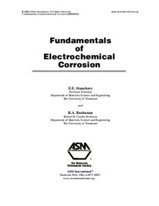
Figure 12.6: Potential distribution for an n-GaAs electrode in contact with a selenium redox couple with fast interfacial reactions: curve a in the absence of illumination; curve b at open circuit with 882 W/m2 illumination; and curve c under illumination near the short-circuit condition (-23.1 mA/cm2). The Debye length in the electrolyte was 0.2 nm, and the Debye length in the semiconductor was 70 nm. (Taken from Orazem and Newman.161)
driving force. Under illumination at open-circuit (curve b in Figure 12.6), electronhole pairs generated by the light are separated by the electric field, resulting in a straightening of the bands. The accumulation of electrons and holes creates an electric field that tends to oppose the field formed at equilibrium. The difference between the potential at equilibrium and under illumination at open-circuit represents the driving force for flow of electrical current. The potential distribution under illumination and near the short-circuit condition (curve c in Figure 12.6) tends to approach the equilibrium distribution. All the variation in potential takes place within the semiconductor. The potential drop across the electrolyte is comparatively insignificant. The selection of a reference potential at the Ohmic contact is arbitrary and was chosen to emphasize the degree of band bending and straightening in the semiconductor. The development of Mott-Schottky theory in Section 12.3.2 employs a potential referenced to the Ohmic contact. A difference in sign will be seen if the potential is referenced instead to a reference electrode located in the electrolyte. The potential of the electrolyte has been found to be independent of current and illumination intensity when referenced to an external quantity such as the Fermi energy of an electron in vacuum.162*163 This concept has proved useful for predicting the interaction between semiconductors and a variety of redox couples. The IUPAC standard for photoelectrochemical systems, in fact, is that the potential is referred to a reference electrode in the ele~trolyte.l@t~~~ The potential distributions in Figure 12.6 can be interpreted in terms of the associated concentration distributions for electrons and holes presented in Figure 12.7.
12.3 IMPEDANCE MODELS
223
The linear scale presented in Figure 12.7(a)emphasizes the depletion of electrons near the interface and the corresponding increase in hole concentrations. The logarithmic scale presented in Figure 12.7(b)emphasizes the change in electron and hole concentrations over many orders of magnitude. Under equilibrium conditions (curve a in Figure 12.7), the hole concentration is very small far from the interface but increases near the negatively charged interface. Conduction-band electrons are depleted near the interface but reach a value close to the net dopant concentration (Nd- N o ) in the electrically neutral region far from the interface. As shown by curve a in Figure 12.7, the equilibrated semiconductor can be described as having an inversion region from the interface to y / h s c = 3, in which the minority carrier concentration exceeds that of the majority carrier, a depletion region from y / h s , = 3 to y/h,, = 8, in which the scaled majority carrier concentration is smaller than unity, and an electrically neutral region extending beyond y / h , , = 8. These positions can be compared to the potential distribution given by curve a in Figure 12.6. As shown by curve b in Figure 12.7, illumination at the open-circuit condition produces electron-hole pairs that are separated by the potential gradient associated with the interface. The concentration of holes increases at all positions within the semiconductor, and the concentration of electrons increases in the space-charge region, thus straightening the equilibrium potential variation. As the system approaches the short-circuit condition under illumination (curve c in Figure 12.7),the concentrations of electrons and holes tends toward the equilibrium distributions.
12.3
Impedance Models
Numerical solutions have been presented for the impedance response of semiconducting systems that account for the coupled influence of transport and kinetic phenomena, see, e.g., Bonham and Orazem.166r167Simplified electrical-circuit analogues have been developed to account for deep-level electronic states, and a graphical method has been used to facilitate interpretation of high-frequency measurements of capacitance. The simplified approaches are described in the following sections. 12.3.1
Equivalent Electrical Circuits
Sah and coworkers have developed a quasi-analytic calculation that can be expressed as a detailed equivalent electrical This development is summarized by Jansen et al.17’ and used to justify the application of the simplified equivalent circuit shown in Figure 12.8 to the analysis of the impedance response of semiconductors containing deep-level electronic states. This circuit was used to analyze the impedance data presented in Section 18.2 (see, e.g., Figure 18.4). In Figure 12.8, C, is the space-charge capacitance, R, is a resistance that accounts for a small but finite leakage current,17s175 and the parameters R1 . . . Rk and C1 . . . ck are attributed to the response of discrete deep-level energy states.
224
SEMICONDUCTING SYSTEMS CHAPTER 12
3l I'
Ib
n
?m
2"
W
\
0
2
1
I
1
electrons ---
I
holes
I I I
1 I
I
t 7,:
W
\
0
Figure 12.7: Concen-.ation distributions for electrons (solid lines) and holes (dashed lines) for an n-GaAs electrode in contact with a selenium redox couple with fast interfacial reactions: curve a in the absence of illumination; curve b a t open circuit with 882 W/m2 illumination; and curve c under illumination near the short-circuit condition (-23.1 mA/cm2). Concentrations were scaled t o the net dopant concentration (Nd - Na):a) concentrations given in a linear scale; and b) concentrations given in a logarithmic scale. (Taken from Orazem and Newman.161)
12.3 IMPEDANCE MODELS
w 3 R,
225
:
in Figure 12.8: Electrical circuit corresponding t o the model presented by Jansen e t which Cn is the spacecharge capacitance, Rn is a resistance that accounts for a small but finite are attributed t o the response of leakage current, and the parameters R1 . . Rk and C1 . . . discrete deep-level energy states.
.
ck
Similar circuits have been used to account for both h o m o g e n e o ~ s and ' ~ ~in~~~ terfacial electronic s t a t e ~The . ~circuit ~ ~ shown ~ ~ ~ in~ Figure 12.8 cannot be used to distinguish between surface and bulk deep-level states. It is possible to distinguish the two types of states by means of the Mott-Schottky plots described in Sections 12.3.2 and 18.3. 12.3.2
Mott-Schottky Analysis
Graphical techniques can be applied for single-frequency measurements when the frequency selected excludes the contributions of confounding phenomena. For example, impedance measurements on a semiconductor diode at a sufficiently high frequency exclude the influence of leakage currents and of electronic transitions between deep-level and band-edge states. Thus, as discussed in Section 16.4, the capacitance can be extracted from the imaginary part of the impedance as 1
(12.22)
The problem is reduced to one of identifying the relationship between semiconductor properties and the capacitance as a function of applied potential. The capacitance of the space-charge region C is determined through (12.23)
where the charge density of the space-charge region qx is related to potential through Poisson's equation (12.20). Solution of equation (12.20) is facilitated by
226
SEMICONDUCTING SYSTEMS CHAPTER 12
expressing the concentration of electrons and holes in terms of potential through insertion of equations (12.14)and (12.13)into the Boltzmann distributions for electrons and holes, equations (12.7) and (12.8), respectively. Thus, Poisson's equation can be expressed as (12.24) where @ is the electrostatic potential, (Nd - Nu)is the doping level, and P and N are the hole and electron concentrations, respectively, at the flat-band potential. Deep-level states were not included in the expression for charge density. The occupancy of deep-level states is a function of potential, and a similar development can be made to take such states into account.180 The charge density used in equation (12.24) (12.25) p,(@) = F [Pe-FOlRT - NeFQ/RT+ (Nd - NU)] is now an explicit function of potential rather than position. Equation (12.25) can
be compared to the definition provided as equation (12.10). Integration of Poisson's equation is facilitated by posing equation (12.24) in terms of the electric field (12.26)
dY
The second derivation of potential with respect to position can be expressed in terms of a derivative with respect to potential as d2@ = -dE = --dEd@ -
dy*
Thus, Integration yields
dy
a@ dy
1dE2 = E-dE = -a@ 2 d@
d E2 2 = --px(@) d@
EEO
E2 = --2 EEO
(12.27)
(12.28)
9
J px(@)d@
(12.29)
9fb
where the flat-band potential @fi is the potential in the electrically neutral region far from the interface. The charge held within the space-charge region is given by (12.30)
m R e m e m b e r ! 12.4 Mott-Shottky theory provides a relationship between the expm'mentally measured capacitance, the doping level, and theflat-band potential.
227
12.3 IMPEDANCE MODELS
Under the assumption that there are no surface states or specific adsorption of charged species, the space charge 4% in a semiconductor in contact with an electrolyte is balanced by the charge in the diffuse part of the double layer q d ; thus, 4% = q d . Gauss's law can therefore be used to provide a boundary condition for the electric field at the surface of the semiconductor as (12.31)
Thus qsc
= EEOE(@(O))
(12.32)
The space-charge capacitance is given by (12.33)
or (12.34)
Equation (12.34) provides a relationship between the capacitance of the spacecharge region of the semiconductor, the electric field at the interface, and the charge density at the interface. Under the convention that the potential is referenced to the flat-band potential @h, i.e., the potential is equal to zero far from the interface where the electric field is also equal to zero, integration of equation (12.29) yields
A general expression for capacity can be found to be
The values for N and P can be evaluated at the flat-band potential under the assumptions of equilibrium (i.e., np = n;) and electroneutrality (i.e., psc = 0). (12.37)
and
P= 2
[- ( N d - Na)1+-4
(12.38)
Equations (12.37) and (12.38) can be inserted into equation (12.36) to provide a n expression for capacitance as a function of potential, with doping level as a parameter.
228
SEMICONDUCTING SYSTEMS CHAPTER 12
4
.
,
.
,
.
,
.
I
.
,
.
Figure 12.9: Calculated capacitance for a GaAs Schottky diode (see Table 12.1 for relevant parameten for GaAs semiconductors): a) capacitance as a function of potential referenced to the flat-band potential for an intrinsic semiconductor: and b) l/C:c as a function of potential referenced to the flat-band potential for a lightly doped p-type semiconductor.
The capacitance is presented in Figure 12.9(a)for an intrinsic GaAs semiconductor diode. Some relevant physical properties of GaAs are presented in Table 12.1. The capacitance is symmetric with respect to potential referenced to the flatband potential. At modest doping levels, as shown in Figure 12.9(b) for p-type semiconductors, the plot of 1/C& has a significant linear portion with respect to potential. At more positive potentials, the plot deviates from a straight line due to the contribution of minority carriers. Mott-Shottky plots of 1/C& as a function of potential are particularly useful at larger doping levels. Calculated values for l/C& are presented in Figure 12.10(a) for a GaAs diode with potential referenced to the Ohmic contact, as was used in Figure 12.6. The corresponding values are presented in Figure 12.10(b) for potentials referenced to a reference electrode located in the electrolyte in accordance with the IUPAC convention for semiconductor e l e c t r o d e ~ . The ~ ~ /principal ~ ~ ~ distinction between the two plots is that the positive slopes correspond to a p-type semiconductor in Figure 12.10(a)and to an n-type semiconductor in Figure 12.10(b). All concentration terms were included in the analysis. As seen in Figure 12.10, l/C& is linear over a broad range of potential. The linear portion for Figure 12.10(a)is given by -1= -
2(@(0)-
+ RT/F)
&&OF(% - Nu)
CL
(12.39)
for an n-type semiconductor and by
- 1_ -C&
for a p-type semiconductor.
2(@(0)- @fi
- RT/F)
&EOF(Nd- Nu)
(12.40)
12.3 IMPEDANCE MODELS
229
t
J
s \
S Y
0
Figure 12.10: Mott-Schottky plot of l / C & as a function of potential referenced t o the flatband potential for a GaAs Schottky diode: a) potential referenced t o the Ohmic contact; and b) potential referenced t o a reference electrode located in the electrolyte according t o the IUPAC convention for semiconductor 165
Example 12.1 Mott-Schottky Plots: Beginning with equation (22.36), derive equation (22.39)for an n-type semiconductor. Solution: For an n-type semiconductor, (Nd - Na) is positive and much larger than the intrinsic concentration ni; thus, N + (Nd - Na) and P -+ 0. In the denominator, Pexp(-F@(O)/RT) can be neglected. In the numerator, P (exp(-F@(O)/RT) - 1) can also be neglected. The linear portion of the cume lies at negative potentials, referenced to thefiat-band potential; thus, exp(F@(O)/RT)--t 0 and N(exp(-F@(O)/RT) - 1) M - (Nd - Na)
(12.41)
Equation (22.36) can be expressed as (12.42) (12.43) A similar development at positive potentials will yield equation (22.40).
The assumptions implicit in the Mott-Schottky theory are: 0
The potential is restricted to the range where both the majority (in this case, electrons) and the minority carriers (holes) are negligible as compared to the doping level. These constraints are violated at small and large magnitudes of potential (referenced to the flat-band potential), respectively. This potential range becomes increasingly restrictive as the doping level decreases, and the technique is unusable for semi-insulating materials.
230 0
0
SEMICONDUCTINGSYSTEMS CHAPTER 12
The semiconductor electrode must be ideally polarizable over the potential range of interest. This means that there is no leakage current or Faradaic reaction to allow charge transfer across the semiconductor-electrolyte interface. This restriction is not too important if measurements are taken at sufficiently high frequency that the effects of Faradaic reactions are suppressed. Electron and hole concentrations follow a Boltzmann distribution, i.e., activity coefficient corrections can be neglected.
Equations (12.39)and (12.40)form the basis of a method, described in Section 18.3, used to extract doping levels and flat-band potentials for semiconducting materials. Problems
12.1 Develop the relationship needed to convert the mobility given in Table 12.1, e.g., pn, to diffusivity. 12.2 Calculate the Debye length in units of pm expected for an n-type GaAs semiconductor with a dopant concentration of Compare the value you obtain to the Debye length obtained for an electrolytic system with a NaCl concentration of 0.1 M. 12.3 Plot the equilibrium concentration and potential distribution in the spacecharge region of an n-type GaAs semiconductor (doped cmd3) if the electron concentration at the surface is 20 orders of magnitude less than the bulk concentration. Use semilogarithmic plots for concentration and linear plots for potential. 12.4 The capacity of the space-charge region can be related to the dopant concentration (or fixed charge) in a semiconductor. The space-charge region is essentially equivalent to the diffuse double layer treated in electrolytes with the exception that ionized impurities are present that, at room temperatures, are immobile. For this case, Poisson’s equation becomes (12.44)
Show that the capacity can be related to doping level (Nd - N a ) and potential by the Mott-Schottky relationship (12.45) 12.5 Deviations from straight lines in Mott-Schottky plots can be attributed to the influence of potential-dependent charging of surface or bulk states. This interpretation is supported by analytic calculations of the contribution of defects to the space charge as a function of applied potential. In principle, the
PROBLEMS
231
effect of applied potential of the state of charge of defects can be used to determine the distribution of defects within the space-charge region. Apply the Fermi-Dirac distribution function to the defects to obtain a relationship for the space-charge capacitance for a semiconductor that is sufficiently n-type that the contribution of holes to the charge can be regarded to be negligible. 12.6 Changes in space-charge capacity can be used to observe the effect of charging and discharging of electronic states in a semiconductor subject to subbandgap illumination. Show that the change in observed capacity caused by illumination can be referenced to the unilluminated case by (12.46)
where A c i is the change in the state of charge of the interband state caused by illumination. It is clear from this problem that identification of defects by this method requires excellent resolution for moderate doping levels and that the concentration measured in this way is the change in the state of charge of the defect, not the actual defect concentration. 12.7 The capacity of the electrolytic diffuse double layer is often ignored when Mott-Schottky plots are used to characterize semiconductor-electrolyte interfaces. Under what conditions is this assumption justified? 12.8 Mott-Schottky plots are often generated by using measurements at a single frequency, often 1kHz.Explain the limitations of this approach. 12.9 A claim is made in Section 12.3.1 that Mott-Schottky plots may be used to distinguish between surface and bulk deep-level states. Explain how this may be accomplished.
Electrochemical Impedance Spectroscopy by Mark E. Orazem and Bernard Tribollet Copyright 02008 John Wiley& Sons, Inc.
Chapter 13 Time- Constant Dispersion The impedance models developed in Chapters 9,10,11, and 12 are based on the assumption that the electrode behaves as a uniformly active surface where each physical phenomenon or reaction has a single-valued time constant. The asswnption of a uniformly active electrode is generally not valid. Time-constant dispersion can be observed due to variation along the electrode surface of reactivity or of current and potential. Such a variation is described in Section 13.1.1 as resulting in a 2-dimensional distribution. Time-constant dispersion can also be caused by a distribution of time constants that reflect a local property of the electrode, resulting in a 3dimensional distribution. The presence of time-constant (or frequency) distribution is frequently modeled by use of a constant-phase-element(CPE), discussed in Section 13.1. As discussed in Section 13.1.3, use of a CPE assumes a specific distribution of time constants that may apply only approximately to a given system. The objective of this chapter is to describe specific situations for which time-constant dispersion can be predicted based on fundamental phenomena such as are associated with distributions of mass-transfer rates and Ohmic currents.
13.1 Constant-Phase Elements The impedance response of electrodes rarely show the ideal response expected for single electrochemical reactions. The impedance response typically reflects a distribution of reactivity that is commonly represented in equivalent electrical circuits as a constant phase element (CPE).3g71g'04For a blocking electrode, the impedance can be expressed in terms of a CPE as 1
(13.1)
The impedance associated with a simple Faradaic reaction without diffusion can be expressed in terms of a CPE as Z ( W )= Re
+ 1+ ( j WRt) a Q R t
(13.2)
234
TIME-CONSTANT DISPERSION CHAPTER 13
Figure 13.1: Schematic representation of an impedance distribution for a blocking disk electrode where ze(r) represents the local Ohmic impedance, Co(r) represents the interfacial capacitance, and Qo(r) and &(r) represent local CPE parameters: a) 2-dimensional distribution; and b) combined 2-dimensional and 3-dimensional distribution.
In both equations (13.1) and (13.2), the parameters a: and Q are independent of frequency. When a: = 1, Q has units of a capacitance, i.e., F/cm2, and represents the capacity of the interface. When a # 1, Q has units of sa/ncm2 and the system shows behavior that has been attributed to surface or to continuously distributed time constants for charge-transfer rea~tions.l~*'~~ Independent of the cause of CPE behavior, the phase angle associated with a CPE is independent of frequency. Different expressions for a CPE have been presented in the literature,ls8e.g., Z ( W )= Re
1 +(iW.ro)"
(13.3)
where the parameter 70 is a characteristic time constant for the distribution. Brug et al.lM used a formula in which Q was defined to be in the numerator of equation (13.1)rather than the denominator. The formulas presented in this chapter as equations (13.1)and (13.2)have the advantages that Q is proportional to the active area and the definition of Q for a: = 1is simply the capacitance. 13.1.1
2-D and 3-0 Distributions
Time-constant dispersion leading to CPE behavior can be attributed to distributions of time constants along either the area of the electrode (involving only a 2-dimensional surface) or along the axis normal to the electrode surface (involving a 3-dimensional aspect of the electrode). A 2-D distribution could arise from surface heterogeneities such as grain boundaries, crystal faces on a polycrystalline electrode, or other variations in surface properties. As shown in Section 13.3, the time-constant dispersion associated with geometry-induced nonuniform current and potential distributions results from a 2-D distribution. A schematic representation of a 2-D distribution for an ideally polarized disk electrode is presented in Figure 13.1(a).For a 2-D distribution, the circuit parameters, e.g., capacitance and Ohmic resistance, could be a function of radial position
235
13.1 CONSTANT-PHASE ELEMENTS
along the electrode. The global admittance is obtained by integration of the admittance associated with these circuit elements over the electrode area, i.e., (13.4) where A is the electrode area, Y is the global admittance, Z is the global impedance, and z is the local impedance. Depending on the nature of the local distribution, equation (13.4) may yield a global impedance with a CPE behavior. The local impedance, in the case of a 2-D distribution, would, however, show ideal RC behavior. CPE behavior may also arise from a variation of properties in the direction that is normal to the electrode surface. Such variability may be attributed, for example, to changes in the conductivity of oxide layers189-191(see Section 13.5) or from porosity or surface roughness (see Section 13.4).192g193 This CPE behavior is said to arise from a 3-dimensional distribution, with the third direction being the direction normal to the plane of the electrode.lg4 A 3-D distribution of blocking components in terms of resistors and constantphase elements is presented in Figure 13.1@).Such a system will yield a local impedance with a CPE behavior, even in the absence of a 2-D distribution of surface properties. If the 3-D system shown schematically in Figure 13.l@)is influenced by a 2-D distribution, the local impedance should reveal a variation along the surface of the electrode. Thus, local impedance measurements can be used to distinguish whether the observed global CPE behavior arises from a 2-D distribution, from a 3-D distribution, or from a combined 2-D and 3-D distribution. Equations (13.1) and (13.2) embody an implicit assumption that the RC time constant is not, in fact, a constant but, rather, a parameter that follows a specific distribution. Equation (13.1), for example, can be imagined as arising from a 2-D distribution of time constants q = (ReCo)i,e.g., 1
1
1
00
-,-
.
(13.5)
If T is a continuous function, equation (13.5) can be written ado4 (13.6)
where G(z) is the distribution function of tion of a function of In(.r/.ro),i.e.,
7,
which represents a normal distribu-
1 Sin(lYTC) G(7) = 2TC7cosh (1- a ) In($)] - COS(IYTC)
[
(13.7)
A similar development can be made for equation (13.2), also leading to equation (13.7).
236
TIME-CONSTANT DISPERSION CHAPTER 13
13.1.2
Determination of Capacitance
It is incorrect to equate the CPE parameter Q to the interfacial capacitance. A number of researchers have explored the relationship between CPE parameters and the interfacial capacitance. Hsu and Mansfeldlg5proposed
(13.8) where urnax (or Kmm) is the characteristic frequency at which the imaginary part of the impedance reaches its maximum magnitude and Ceffis the estimated interdeveloped a relationship for a blocking electrode facial capacitance. Brug et between the interfacial capacitance and the CPE coefficient Q as (13.9)
A similar relationship between the interfacial capacitance and the CPE coefficient Q was developed for a Faradaic system as
[ (ie - + - it)( ] a-1)
Ce f fQ
l/a
(a-1)
=
[Q($
(I+?))
]
l/a
(13.10)
For CPE behavior caused by 2-D distributions of current and potential on a disk electrode, equations (13.9) and (13.10) provided the most reliable estimate for interfacial capacitance (see Section 13.3).97Similar formulas for 3-D distributions do not exist. 13.1.3
Limitations to the Use of the CPE
As compared to a parallel combination of a resistor and capacitor, the CPE is able to provide a much better fit to most impedance data. The CPE can achieve this fit using only three parameters, which is only one parameter more than a typical RC couple. Some investigators allow 1y to take values from -1 to 1, thus treating the CPE as an extremely flexible fitting element. For a: = 1, the CPE behaves as a capacitor; for 1y = 0, the CPE behaves as a resistor; and for 1y = -1 the CPE behaves as an inductor (see Section 4.1.1). It must be emphasized that the mathematical simplicity of equations (13.1)and (13.2) is the consequence of a specific time-constant distribution. As shown in this chapter, time-constant distributions can result from nonuniform mass transfer, geometry-induced nonuniform current and potential distributions, electrode porosity, and distributed properties of oxides. At first glance, the associated impedance responses may appear to have a CPE behavior, but the frequency dependence of the phase angle shows that the time-constant distribution differs from that presented in equation (13.7). There are, therefore, two primary concerns with the use of the CPE for modeling impedance data:
13.2 CONVECTIVE DIFFUSION IMPEDANCE AT SMALL ELECTRODES
237
1. While assumption that the time constant is distributed can be better than assuming that the time constant has a single value, the physical system may not follow the specific distribution implied in equation (13.7). The examples presented in the subsequentsections illustrate systems for which a time-constant dispersion results that resem'bles that of a CPE, but with different distributions of time constants. 2. A satisfactory fit of a CPE to experimental data may not necessarily be correlated to the physical processes that govern the system. As shown in Section 4.4,models for impedance are not unique; thus, an excellent fit to the data does not in itself guarantee that the model describes correctly the physics of a given system.
The graphical methods described in Chapter 17 can be used to determine whether a system follows CPE behavior in a given frequency range.
13.2 Convective Diffusion Impedance at Small Electrodes Small electrodes are currently used to study fast electrochemical kinetics or as flow measurement devices in chemical engineering systems. In the latter case, the first experimental and theoretical studies appeared in the early fifties. The goal of these studies was to achieve probes sensitive to the local wall velocity gradient BY =
avx ay
(13.11)
The well-known property of those probes is that the limiting diffusion current is proportional to under steady-state conditions.196For use in electrochemical engineering, an increasing interest is now focused on the nonsteady behavior of those small electrodes under conditions of fluctuating velocity gradient By( t ). Theoretical developments show that it is possible to deduce hydrodynamic information from the limiting current measurement, either in quasi-steady state where I(t ) cx &I3 ( t ) or, at higher frequency, in terms of spectral analysis. In the latter case, it is possible to obtain the velocity spectra from the mass-transfer spectra, where the transfer function between the mass-transfer rate and the velocity perturbation is known. However, in most cases, charge transfer is not infinitely fast, and the analysis also requires knowledge of the convective-diffusion impedance, i.e., the transfer function between a concentration modulation at the interface and the resulting flux of mass under steady-state convection.
IR)Remember! 13.1 While use of a CPE may lead to improved regressions, the meaning can be ambiguous, and the physical system may not follow the specific distribution implied in the CPE model.
238
TIME-CONSTANT DISPERSION CHAPTER 13
Figure 13.2: Schematic representation of flow past a small electrode where the coordinate y is in the direction perpendicular t o the plane of the electrode (x,y).
13.2.1 Analysis A schematic representation of a small electrode embedded in an insulating wall is given in Figure 13.2 on which a fast electrochemical reaction occurs under masstransport limitation, i.e., ci(0) = 0. The length of this electrode in the mean flow direction is small enough that the diffusion layer thickness Si is very small, thus minimizing the effect of the normal velocity component. The normal velocity is proportional to y2, whereas the longitudinal velocity component is proportional to y, where y is the coordinate normal to the wall. Under these conditions, the boundary layer approximations apply. Using a local frame of reference ( x , y) attached to the electrode, the mass conservation equation governing the concentration distribution Ci of a species transported by convective diffusion can be expressed as (13.12)
where v, = BYy. For simplification, the electrode can be considered to be sufficiently small that the flow is uniform in the diffusion layer and By is independent of the space coordinates. The time-average solution for the concentration distribution has been given by L h 4 q ~ e . As l ~shown ~ in Example 2.2, the concentration in the diffusion layer can be expressed as (13.13)
where 32/3r(4/3)4 represents the local value of the diffusion layer thickness with Si = ( D ~ X / B ~ ) '0/ ~5, x 5 L, and Ci(W) is the concentration in the bulk. On a small rectangular electrode of width W, the steady flwc is
-
Ni = W
or
I
L
azi
Di-dx
aY
=
31'3 (Ci(m) - Ci(0)) Di213 By 1/3~2/3w
2r (4/3)
(13.14)
13.2 CONVECTIVE DIFFUSION IMPEDANCE AT SMALL ELECTRODES
239
Equation (13.15) shows that the steady mass-transfer-controlled flux-of a reacting species is proportional to the cube root of the velocity gradient, i.e., Ni cx
A E x m p l e 13.1 Flux on a Small Circular Electrode: Derive an expressionfor the steadyflux on a circular small electrode of radius R. Solution: Equation (13.13) can be used to calculate theflux on a circular small electrode by summing along z, the efect of elementary rectangular strips. In this case, x contained in the definition of Si must be replaced by ( x - XI), which actually corresponds in the local Cartesianframe of r&ence to the distanceporn the leading edge of any elementary strip. The position of the leading edge x1 (z) is afunction of R and z as XI (2)
=R -
d R 2 - z2
(13.16)
Thus,the expression 4 theflux is (13.17)
or
2/3 1/3 2 ~ ) 5 / 3 3ll3(ci(m)- C i ( 0 ) ) Di By ( Ncix = 0.84
2 r (4/3)
(13.18)
Comparison with equation (13.14)reveals that theflux at a circular electrode is 84 percent smaller than that at a square electrode with L = W = 2R. 13.2.2
Local Diffusion Convective Impedance
The nonsteady part of the mass balance equation (13.12) may be written as: (13.19)
The boundary conditions for the nonsteady equations are
6 = G(0) aG -= O aY
6 =0
for y = 0 and x 2
XI
for y = O and x 2 x1 for y
4 0 0
(13.20)
and all x
A dimensionless concentration 8i can be defined such that
(13.21)
The dimensionless normal distance to the wall can be defined to be (13.22)
240
TIME-CONSTANT DISPERSION CHAPTER 13
where x1 is the coordinate of the leading edge of the electrode as shown in Figure 13.2. Equation (13.22) represents a similarity variable (see Section 2.4). Introduction of q into equation (13.19) results in definition of a dimensionless positiondependent frequency given by (13.23)
In terms of equations (13.21)to (13.23), equation (13.19)becomes (13.24)
The spatial dependence of the sinusoidal perturbation is evident in the definition of Kx,i. As Kx,i contains a dependence on the space coordinates, it is necessary to derive first the local solution. A solution in the form of a series can be obtained as (13.25) For this solution the number of terms that play a role in the series increases with the frequency. Generally the solution given by equation (13.25) is used for the lowfrequency solution, and the high-frequency solution is derived by another method. Low-Frequency Solution
The elementary functions hm ( q) are real and obey (13.26) and (13.27) The boundary conditions at q = 0 are @(O) = 1, ei,o(O) = 1, and &,,(O) = 0 for all m > 0. The boundary condition at q + 00 is h ( m ) = 0. In fact, since the only observable quantity is the interfacial flux, only its expression is needed, i.e., (13-28) The terms dOi,m/dq(oare tabulated by Deslouis et al.I9’ for 0 5 m 5 79.
241
13.2 CONVECTIVE DIFFUSION IMPEDANCE AT SMALL ELECTRODES
II
II
II
II
-
-
0.25
0.5
REAL PART
0.75
1
Figure 13.3: Local normalized diffusion impedance for the small electrode given in Figure 13.2. The solid line represents the low-frequency solution (equation (13.28)),and the dashed line represents the high-frequency solution (equation (13.31)). Overlap is obtained for 6 5 K , i 5 13, with the dimensionless frequency K , i given by equation (13.23). (Taken from Delouis e t and reproduced with permission of The Electrochemical Society.)
High-Frequency Solution
Since the concentration modulation is rapidly damped close to the wall at high frequencies, the convective term can be disregarded and equation (13.24) becomes (13.29)
The solution to equation (13.29) can be found using the methods described in Section 2.2. Due to the boundary conditions (Oi = 0 when 7 + 00 and Oi = 1 when 7 = 0), the analytic solution is, as given for equation (11.46), (13.30)
The local dimensionless impedance is obtained as (13.31)
which is a normalized Warburg impedance as described in Section 11.3. As seen in Figure 13.3, the high-frequency solution (13.28) and the low-frequency solution (13.31) present a satisfactory overlap for 6 I K , i 5 13.
242
13.2.3
TIME-CONSTANT DISPERSION CHAPTER 13
Global Convective Diffusion Impedance
The dimensionless impedance of a small electrode can be defined by summing the effects of the local convective-diffusion impedance, i.e.,
For a rectangular electrode of length L and of width W, the expression of the impedance is given by (13.33)
By using the dimensionless frequency (13.34)
equation (13.33)can be expressed as (13.35)
with (13.36)
In the low-frequency range, the expression of H ( K i ) is obtained from the series (13.37)
In the high-frequency range, the integration must be split in two parts since the leading edge of an electrode will be always under a low-frequency regime. Indeed, the local thickness of the diffusion layer, equal to 3 2 / 3 r ( 4 / 3 ) 4 ( x and ) thus x1l3, is very small at the leading edge, and K,,i remains there alproportional to ways small even for high values of w / 2 n . Thus, (13.38)
The first integral corresponds to the low-frequency regime and the second one to the high-frequency regime where equations (13.28) and (13.31) must be used, respectively. Equation (13.38)becomes (13.39)
13.3 GEOMETRY-INDUCED CURRENT AND POTENTIAL DISTRIBUTIONS
243
REAL PART Figure trode. dashed for 6 5 Delouis
13.4: Normalized global convectivediffusion impedance for a small rectangular elecThe solid line represents the low-frequency solution (equation (13.37)), and the line represents the high-frequency solution (equation (13.40)). Overlap is obtained Ki 5 13, with the dimensionless frequency Ki given by equation (13.34). (Taken from et and reproduced with permission of The Electrochemical Society.)
The term B (0-1) has been calculated for 0-1 5 13, and B (q) was found to be constant and equal to 0.25j in the frequency range 6 5 ~1 5 13. This result means that equation (13.39) is valid for Ki 2 6 and therefore can be written as 0.25j H(Ki) = -Ki
+ (jKi)1’2
(13.40)
As a consequence, a fair overlap between equation (13.37) and equation (13.40) is obtained for 6 5 Ki 5 13 as shown in Figure 13.4.
13.3 Geometry-Induced Current and Potential Distributions The geometry of an electrode frequently constrains the distribution of current density and potential in the electrolyte adjacent to the electrode in such a way that both cannot simultaneously be uniform. The primary and secondary current and potential distributions associated with a disk embedded in an insulating plane, originally developed by Newman,198n199are presented in Section 5.6. The potential distribution on the disk electrode is not uniform under conditions where the current density is uniform and, conversely, the current distribution is nonuniform under the primary condition where the solution potential is uniform. The nonuniform current and potential distribution associated with the disk geometry influences the transient and the impedance response. Nisancioglu and
m R e m e m b e r ! 13.2 Not all time-constant distributions give rise to a CPE.
244
TIME-CONSTANT DISPERSION CHAPTER 13
Newman200j201 modeled the transient response of a disk electrode to step changes in current. The solution to Laplace’s equation was performed using a transformation to rotational elliptic coordinates and a series expansion in terms of Lengendre polynomials. Antohi and Scherson expanded the solution to the transient problem by expanding the number of terms used in the series expansion.202 The geometry-induced current and potential distributions cause a frequency or time-constant dispersion that distorts the impedance response of a disk electrode.38~2039204 Huang et al?7~1021205 have shown that current and potential distributions induce a high-frequency pseudo-CPE behavior in the global impedance response of a disk electrode with a local ideally capacitivebehavior, a blocking disk electrode exhibiting a local CPE behavior, and a disk electrode exhibiting Faradaic behavior. 13.3.1
Mathematical Development
The mathematical development presented here follows that presented by Newman.” The development in terms of rotational elliptic coordinates, i.e.,
Y = rot7
(13.41)
and
r = rod-
(13.42)
was summarized by Huang et al. for blocking e l e c t r o d e ~ . l ~ ~ # ~ ~ ~ The problem was solved for two kinetic regimes. Under linear kinetics, following Newman” and N i s a n c i ~ g l uthe~ current ~ ~ ~ ~density ~ at the electrode surface could be expressed as
i
= Co
a ( v - oo) (aa+ a c ) OF (V - QO) at RT +
(13.43)
The assumption of linear kinetics applies for f io, the parameter J was defined to be a function of radial position on the electrode surface as
+
(13.49)
where i( 7) was obtained from the steady-state solution as
The local charge-transfer resistance for linear kinetics can be expressed in terms of parameters used in equation (13.48) as (13.51)
The local charge-transfer resistance for Tafel kinetics can be expressed in terms of parameters used in equation (13.49)as (13.52)
For linear kinetics, Rt is independent of radial position, but, under Tafel kinetics, as shown in equation (13.52),Rt depends on radial position. From a mathematical perspective, the principal difference between the linear and Tafel cases is that J and Rt are held constant for linear polarization; whereas, for the Tafel kinetics,
246
TIME-CONSTANT DISPERSION CHAPTER 13
J and Rt are functions of radial position determined by solution of the nonlinear steady-state problem. The relationship between the parameter J and the charge-transfer and Ohmic resistances can be established using the high-frequency limit for the Ohmic resistance to a disk electrode obtained by Newman,lg8i.e., (13.53) where Re has units of ncm2. The parameter J can therefore be expressed in terms of the Ohmic resistance Re and charge-transfer resistance Rt as (13.54) Large values of J are seen when the Ohmic resistance is much larger than the charge-transfer resistance, and small values of J are seen when the charge-transfer resistance dominates. 13.3.2
Global and Local Impedances
Following Huang et a1.;O2 a notation is presented in Section 7.5.2 that addresses the concepts of a global impedance, which involved quantities averaged over the electrode surface; a local interfacial impedance, which involved both a local current density and the local potential drop - &(r) across the diffuse double layer; a local impedance, which involved a local current density and the potential of the electrode referenced to a distant electrode; and a local Ohmic impedance, which involved a local current density and potential drop 5 0 ( r ) from the outer region of the diffuse double layer to the distant electrode. The corresponding list of symbols is provided in Table 7.2. The local impedance z can be represented by the sum of local interfacial impedance zo and local Ohmic impedance Ze as Z = ZO
+Ze
(13.55)
Huang et al.1021205demonstrated for blocking disk electrodes that, while the local interfacial impedance represents the behavior of the system unaffected by the current and potential distributions along the surface of the electrode, the local impedance shows significant time-constant dispersion. The local and global Ohmic impedances were shown to contain the influence of the current and potential distributions. While the calculations presented here were performed in terms of solution of Laplace's equation for a disk geometry, the nature of the electrode-electrolyte interface can be understood in the context of the schematic representation given in Figure 13.5. Under linear kinetics, both COand Rt can be considered to be independent of radial position, whereas, for Tafel kinetics, 1/ Rt varies with radial position in accordance with the current distribution presented in Figure 5.10. The calculated results for global impedance, local impedance, local interfacial impedance, and both local and global Ohmic impedances are presented in this section.
13.3 GEOMETRY-INDUCED CURRENT AND POTENTIAL DISTRIBUTIONS
247
Figure 13.5: Schematic representation of an impedance distribution for a disk electrode where Co represents the interfacial capacitance, which in this case can be considered to be associated with the doublelayer, and Rt represents the chargetransfer resistance. (Taken from Huang et ,Isg7 and reproduced with permission of T h e Electrochemical Society.) Ze represents the local Ohmic impedance,
Global Impedance
The calculated real and imaginary parts of the global impedance response are shown in Figures 13.6(a) and (b), respectively. At low frequencies, values for the real part of the impedance differ for impedance calculated under the assumptions of linear and Tafel kinetics, whereas, the values of the imaginary impedance calculated under the assumptions of linear and Tafel kinetics are superposed for all frequencies. The slopes of the lines presented in Figure 13.6(b) are equal to +1 at low frequencies but differ from -1 at high frequencies. As discussed in Section 17.1.3, the slope of these lines in the high-frequency range can be related to the exponent 1y used in models for CPE behavior.206 Following the definition of 1 given in equation (13.49), the curves for 1= 0 in Figures 13.6(a)and (b) correspond to an ideally capacitive blocking electrode. The steady-state solution for the current distribution at a blocking electrode is that the current is equal to zero. The primary current distribution given as equation (5.65) therefore applies, not at the steady state, but at infinite frequency. For the special case of a Faradaic system with an Ohmic resistance that is much larger than the kinetic resistance, J + 00, and equation (5.65) provides the steady-state current distribution. Two characteristic frequencies are evident in Figure 13.6. The characteristic frequency K = 1is associated with the influence of current and potential distributions and can be expressed in terms of the capacitance Co and the Ohmic resistance to a
248
TIME-CONSTANT DISPERSION CHAPTER 13
lo5,
,
1o4
1
lod lo4
,
,
10"
,
1
lo"
,
1
10'
,
1
loo
,
,
1
1
10'
Id los
Figure 13.6: Calculated representation of the impedance response for a disk electrode under assumption of Tafel kinetics with J as a parameter. The value J = 0 corresponds to an ideally capacitive blocking electrode: a) real part; and b) imaginary part.
disk electrode given in equation (13.53) as (13.56) The characteristic frequency K / J = 1is associated with the RtCo-time constant for the Faradaic reaction. The frequency K = 1at which the current and potential distributions begin to influence the impedance response can be expressed as
f=s K
(13.57)
or, in terms of electrolyte resistance, as (13.58) The frequency K = 1 at which the current distribui,m influences the apedance response is shown in Figure 13.7with K/COas a parameter. As demonstrated in Example 13.2, the influence of high-frequency geometry-induced he-constant dispersion can be avoided for reactions that do not involve adsorbed intermediates by conducting experiments below the characteristic frequency given in equation (13.57). The characteristic frequency can be well within the range of experimental measurements. The value K/CO= lo3 cm/s, for example, can be obtained for a capacitance CO = 10 pF/cm2 (corresponding to the value expected for the double layer on a metal electrode) and conductivity K = 0.01 S/cm (corresponding roughly to a 0.1 M NaCl solution). Equation (13.57) suggests that time-constant dispersion should be expected above a frequency of 600 Hz on a disk with radius 10 = 0.25 cm.
13.3 GEOMETRY-INDUCED CURRENT AND POTENTIAL DISTRIBUTIONS
249
r,, / cm Figure 13.7: The frequency K = 1 at which the current distribution influences the impedance response with K / C Oas a parameter. (Taken from Huang et and reproduced with permission of The Electrochemical Society.)
Example 13.2 Characteristic Frequency: Consider an experimental system involving a Pt disk in 0.1 M NaCl solution at room temperaturefor which impedance measurements are desired to a maximumfrequency of 10 kHz. Estimate the maximum radius for a disk electrode that will avoid the influence of high-frequency geomety-induced timeconstant dispersion. Solution: The characteristic frequency given in equation (13.57)depends on the ratio K/CO.The conductivity can be estimated using equation (5.56)and values of difisivity takmfrom Table 5.2. The conductivity can be estimated to be K = 0.013 (ncm)-l. The double-layer capacitance for a bare electrode is of the order of CO = 10 pF/cm2. Thus, K/CO= 1.3 x lo3 cm/s, and,following (13.59)
the maximum disk radius is 0.02 cm. This result can also be obtainedfrom Figure 13.7. Local Interfacial Impedance
For the linear kinetics calculation, where I is independent of radial position, the scaled real part of the local interfacial impedance follows
-ZO,rK
-
r0n
I
n(J2+K2)
(13.60)
and the imaginary part of the local interfacial impedance follows zo,F --
ron
-K n(J2+K2)
(13.61)
250
TIME-CONSTANT DISPERSION CHAPTER 13
Tafel: J = 1.O
-D- r I ro = 0.96
0.0
0.1
0.2
0.3
0.4
0.5
0.6
0.7
0.8
Figure 13.8: Calculated representation of the local impedance response for a disk electrode as a function of dimensionless frequency K under assumptions of Tafel kinetics with J = 1. (Taken from Huang e t al.97 and reproduced with permission of The Electrochemical Society.)
The local interfacial impedance is that associated with the boundary at the electrode surface. For a simple Faradaic system, the local interfacial impedance is that of an resistor in parallel connection to a capacitor and includes no Ohmic resistance. For an ideally capacitive electrode, the local interfacial impedance is that of a capacitor with no real component. Local Impedance
The calculated local impedance is presented in Figure 13.8 for Tafel kinetics with J = 1and with radial position as a parameter. The impedance is largest at the tenter of the disk and smallest at the periphery, reflecting the greater accessibility of the periphery of the disk electrode. Similar results were also obtained for J = 0.1, but the differences between radial positions were much less significant. Inductive loops are observed at high frequencies, and these are seen in both Tafel and linear calculations for J = 0.1 and J = l.0?7 Local Ohmic Impedance
The local Ohmic impedance ze accounts for the differencebetween the local interfacial and the local impedances. The calculated local Ohmic impedance for Tafel kinetics with J = 1.0 is presented in Figure 13.9 in Nyquist format with normalized radial position as a parameter. The results obtained here for the local Ohmic impedance are very similar to those reported for the ideally polarized electrode and for the blocking electrode with local CPE b e h a v i ~ r . l At ~ ~the # ~periphery ~~ of the electrode, two time constants (inductive and capacitive loops) are seen, whereas at the electrode center only an inductive loop is evident. These loops are distributed around the asymptotic real value of 1/4. The representation of an Ohmic impedance as a complex number represents a departure from standard practice. As shown in previous sections, the local impe-
251
13.3 GEOMETRY-INDUCED CURRENT AND POTENTIAL DISTRIBUTIONS
0.1
I
I
e
1
Lo
1
0.0
Y,
I
-Ck r I ro= 0.96 &r I ro = 0.51 O r / ro = 0.80 + p r / ro= 0
K=10
\
I
100
9Ja
Tafel: J = 1.O -0.1
I
1
1
1
1
1
Figure 13.9: Calculated representation of the local Ohmic impedance response for a disk electrode as a function of dimensionless frequency K under assumptions of Tafel kinetics with J = 1. (Taken from Huang e t and reproduced with permission of The Electrochemical Society.)
dance has inductive features that are not seen in the local interfacial impedance. These inductive features are implicit in the local Ohmic impedance. As similar results were obtained for ideally polarizedlo2and blocking electrodes with local CPE behavior?O5 the result cannot be attributed to Faradaic reactions and can be attributed only to the Ohmic contribution of the electrolyte. Global Interfacial and Global Ohmic Impedance
The global interfacial impedance for linear kinetics is independent of radial position and is given by Rt zo = 1 jwCoRt (13.62)
+
The global Ohmic impedance Ze is obtained from the global impedance Z by the expression Ze = Z - ZO (13.63) The real part of Ze, obtained for linear kinetics, is given in Figure 13.10(a), and the imaginary part of Ze is given in Figure 13.10(b)as functions of dimensionless frequency K with J as a parameter. In the low-frequency range ZeK/ron is a pure resistance with a numerical value that depends weakly on J. All curves converge in the high-frequency range such that Z , ~ / r o ntends toward 1/4. The imaginary part of the global Ohmic impedance shows a non-zero value in the frequency range that is influenced by the current and potential distributions.
m)Remember! 13.3 The Ohmic impedance is a complex quantity that is influenced by geometry-induced current and potential distributions.
252
TIME-CONSTANT DISPERSION CHAPTER 13
1o4 1o4
1'0 : o \
Y._
N'
lo* lo* 1v7
1o4 1o4 0.2451
10"
'
10"
'
10'
' ' ' l o 2 10" loo K
(4
'
10'
'
10'
I
lo3
10'O
lo4
10"
loJ
10"
lo-' loo K
10'
10'
10'
(b)
Figure 13.10: Calculated global Ohmic impedance response for a disk electrode as a function of dimensionless frequency for linear kinetics with J as a parameter: a) real part; and b) imaginary part.
At high and low-frequency limits, the global Ohmic impedance defined in this section is consistent with the accepted understanding of the Ohmic resistance to current flow to a disk electrode. The global Ohmic impedance approaches, at high frequencies, the primary resistance for a disk electrode (equation (13.53))described by Newman.19* This result was obtained as well for ideally polarizedloZ and blocking electrodes with local CPE behavior.z05The global Ohmic impedance approaches, at low frequencies, the value for the Ohmic resistance calculated by Newman% for a disk electrode. Again/ this result was seen as well for blocking electrode^.^^^^^^^ The complex nature of the global and local Ohmic impedances is seen at intermediate frequencies. This complex value is the origin of the inductive features calculated for the local impedance and the quasi-CPE behavior found at high frequency for the global impedance.
13.4
Porous Electrodes
Porous electrodes are used in numerous industrial applications because they have the advantage of an increased effective active area. A porous electrode can be obtained by such different techniques as pressing metal powder or dissolution.19z This type of porous electrode structure is also observed on some corroded elect r o d e ~ It. ~is ~important ~ to recognize that a porous electrode is not the same as a porous layer. The structure may be the same, but, while the pore walls are electroactive for a porous electrode, the pore walls are inert for a porous layer. The random structure of the porous electrode, illustrated in Figure 13.11(a), leads to a distribution of pore diameters and lengths. Nevertheless, the porous electrode is usually represented by the simplified single-pore model shown in Figure 13.11(b)in which pores are assumed to have a cylindrical shape with a length t and a radius r. The impedance of the pore can be represented by the transmission
253
13.4 POROUS ELECTRODES
Figure 13.11: Schematic representations of a porous electrode: a) porous electrode with irregular channels between particles of electrode material; and b) transmission line inside a cylindrical pore.
line presented in Figure 13.11(b) where Ro is the electrolyte resistance for one-unit length pore, with units of ncm-l, ZOis the interfacial impedance for a unit length pore, with units of ncm, r is the pore radius in cm, and .t is the pore length in cm. The specific impedances Ro and ZOcan be expressed in function of the pore radius as Ro = P (13.64) m-2
and
7
(13.65) respectively, where Zeq is the interfacial impedance per surface unit, with units of nun2,and p is the electrolyte resistance, with units of Ocm. In the general case, Zo and Ro are functions of the distance x . This dependence is due to the potential distribution or/and to the concentration distribution in the pore. The general solution can be obtained only by a numerical calculation of the corresponding transmission line. For example, the impedance of a porous elec-
Remember! 13.4 A porous electrode is not the same as a porous layer. The structure may be the same, but, while the pore walls are electroactivefor a porous electrode, the pore walls are inertfir a porous layer.
254
TIME-CONSTANT DISPERSION CHAPTER 13
trode in the presence of a concentration gradient was numerically studied by Keddam et a1.208but only a totally irreversible charge-transfer reaction was considered and the Ohmic drop in the pore was neglected. A complete numerical calculation in the presence of a concentration gradient and a potential drop in the pores was developed later by Lasia.209 With the restrictive assumption that ZOand Ro are independent of the distance x , de L e ~ i calculated e~~ analytically the impedance of one pore to be (13-66) The derivation of the de Levie impedance, given in equation (13.66), is presented in Example 13.3. The impedance of the overall electrode is obtained by accounting for the ensemble of n pores and for the electrolyte resistance outside the pore, i.e., (13.67)
The set of equations (13.64)-(13.67) yields an expression for the impedance of the porous electrode Z that is a function of three geometrical parameters t, r, and n as (13.68) The shape of the pores influences the value of the but, in the highfrequency range, this geometrical influence disappears and the impedance is proportional to (Zeq)’l2
Example 13.3 Derivation of the de Levie Formula: Derive the de h i e formula given as equation (13.66). Solution: The transmission line corresponding to transport within a pore is given in Figure 13.11(b). At a distance x from the pore edge, the potential is u ( x ) and the current crossing a resistance Rodx is i ( x ) . 7’he diference of potential at the edges of the resistance is d u ( x ) = Roi(x)dx (13.69) The currentflowing through the impedance Zoldx is given by
di(x) = -dx
ZO
(13.70)
From equations (13.69) and (13.70), the diferential equation d2u - -u Ro dX2 Zo
(13.71)
255
13.4 POROUS ELECTRODES
is obtained. The solution of equation (13.71) is (13.72)
For x = 0, i = 0; thus, A
= B.
The overall current is given by
and the overall impedance is obtained as (13.74)
Equation (13.74)is the de h i e impedance given in equation (13.66). Several limiting behaviors can be seen in equation (13.68). For example, recognizing that (13.75) lim coth(x) = 1 X-mJ
when the argument to the coth function, e ,/-
is sufficiently large,
coth(td2plrZeq) -, 1
(13.76)
and (13.77)
In this particular case, the pores behave as though they are semi-infinitely deep. The parameters r and n cannot be determined separately by regression analysis. Only the product (r3l2n)can be obtained. Other limiting behaviors of equation (13.68) are explored in Problems 13.8 and 13.9.
t
&Example 13.4 Corrosion of Cast Iron in Drinking Water: The internal cor-
rosion rate of drinking water pipes is very small and, in itselfi corrosion is generally not a problem. Butfree chlorine (FCU (the sum of hypochlorous acid HOCl and hypochlorite ions C10-) introduced in water at the treatment plant in order to maintain microbiological quality, gradually disappears throughout the distribution system, which necessitates rechlorination. In order to optimize rechlorination procedures, the diferent sources of chlorine consumption must be identified. The most @en invoked and investigated causes of chlorine decay are the chemical bulk oxidation of organic compounds dissolved in water and the reactions with biofilms on the pipe surface. Furthermore, chlorine reacts with the pipe materials themselves in the corrosion process of cast iron pipes. The corrosion has been invoked as an important source of chlorine decay and thus the corrosion rate must be evaluated.2o7 Derive a model for the impedance response of an iron electrode, taking into
256
TIME-CONSTANT DISPERSION CHAPTER 13
account the material presented in Chapters 9,1 0, and 11 and treating the iron as a porous electrode with poresfilled with corrosion product as shown in Section 9.3.2. Solution: Free chlorine can be directly involved in the corrosion process and reduced at the metal-water interface,following the electrochemical reaction, given for acidic pH by
HOCl
+ Hf + 2e-
2 C1-
+ H20
(13.78)
coupled with the anodic dissolution of ferrous material
+
Fe 2 Fez+ 2e-
(13.79)
On the other hand, chlorine can be chemically reduced by ferrous ions produced by reaction (13.79), according to the homogeneous reaction (inacidic media)
+
2Fe2++ HOCl + H+ F! 2Fe3+ C1-
+ H20
(13.80)
In aerated and chlorinated waters, the rate of reaction (13.78) can be considered to be negligibly small, and the single cathodic process coupled with the dissolution of iron is the reduction of dissolved oxygen, written in acidic media as 1
-2 0 2
+ 2H+ + 2e- 2 H2O
(13.81)
The analysis of the corrosion products suggests the scheme presented in Figure 13.12 for the cast iron-drinking water interface:
On top, the red rust layer explains the absence of hydrodynamic gects after two days of immersion. This layer, which is an electronic insulator but an ionic conductor, does not play any role on the kinetics. Below the reddish layer, an electronically conductive layer of black rust, pictured as an arrangement of macropores, covers the metal except at the end of the pores. The flattened aspect of the diagrams rqflects the presence of this macroporous layer. The black rust is covered by a very compact microporous layer, made up of green rust and calcium carbonates. This film influences the high-frequency loop of the impedance diagrams.
From this physical model, an electrical model of the interface can be given. Free corrosion is the association of an anodic process (iron dissolution) and a cathodic process (electrolyte reduction). %@ore, as discussed in Section 9.2.1, the total impedance of the system near the corrosion potential is equivalent to an anodic impedance Z, in parallel with a cathodic impedance Z , with a solution resistance Re added in series as shown in Figure 13.13(a). The anodic impedance Z , is simply depicted by a double-layer capacitance in parallel with a charge-transfer resistance (Figure 13.13(b)). The cathodic branch is described,following the method of de by a distributed impedance in space as a transmission line in the conducting macropore (Figure 13.12). The interfacial impedance of the microporous
13.4 POROUS ELECTRODES
257
Figure 13.12: Schematic representation of the cast iron - water interface. (Taken from Frateur
e t aI.207)
Figure 13.13: Equivalent circuit for: a) the total impedance of the cast iron-water interface; b) the anodic impedance; and c) the interfacial impedance of the microporous layer.
258
TIME-CONSTANT DISPERSION CHAPTER 13
layer ZOis given in Figure 13.13(c). The term R f represents the Ohmic resistance of the electrolyte through thefilm, and the term C f represents thefilm capacitance. The Ohmic resistance R f is in series with the parallel arrangement of the cathodic double-layer capacitance Cil and the Faradaic branch consisting of a cathodic charge-transfer resistance RF in series with a diffusion impehnce Z D (see also Figure 9.4).The term Z D , which describes the radial diffusion in the macropores, i.e., through the red rust, is given by equation (11.70). Thus,the anodic surface corresponds to the end of the macropores, whereas the cathodic reaction occurs at the end of the micropores, which are located at the walls of the macropores. It should be noted that this physicaklectrical model describes the behavior of cast iron at any time of immersion. The calculation gives, for the cathodic impedance, the general form (13.82)
with (13.83)
and where t is the mean length of the macropores and h is the penetration depth of the electrical signal. When t is small with respect to A, the macropores respond like afzat electrode and the cathodic impedance tends to Z o / t . In this case, the angle made by the diffusion impedance is equal to 45". When t / h becomes large, the macropores behave as though they were semi-infinitely deep. Thus, coth(t/h) tends to unity, and Z, equals which gives an angle of about 22.5" in the so-called Warburg domain. With the model illustrated in Figures 13.12 and 13.13, the impedance diagrams were analyzed by using a nonlinear least-squares regression procedure to extract physically meaningful parameters. For each time of immersion, the electrolyte resistance was measured separately andfixed in order to decrease the number of unknown parameters. The error structures ident$ed by means of the measurement model described in Chapter 21 were used to weight the data during regression of the physical model. The results of thefitting for water containing 2 mg I-' of FC1 after 3, 7, and 28 days of immersion are presented in Figures 13.14(a), (b), and (c), respectively. The model fits the experimental data very well, even under conditions where the diffusion loop is badly dejhed (i.e., at long times of immersion). Therefore, despite the large number of parameters imposed by the physical model, each parameter could be determined with a narrow confidence interval. The calculated diagrams show that the HF loop is, in fact, composed of two capacitive loops: one related to the microporous film and the other to the cathodic charge transfer. Due to the similar values of the time constants RfCil and R f C f , the two corresponding half-circles were nearly indistinguishable. 7'he low-frequency loop characterizes the diffusion of the solute as well as the anodic charge transfer. After 28 days of immersion, the theoretical diagram makes an angle of 45" in the very-high-frequency range and the angle of the diffusion impedance is 22.5", which means that the pores behave as though they are semi-infinitely deep at thesefrequencies.
a,
259
13.4 POROUS ELECTRODES
2
I
1
I
1
1
I
100 rnHz
I
I
39.8 mHz
. B ?j-
, ,* / ,
2.5 mHz
II
0
20
Y
20
-6.3 &Hz
' 1
80
40
Z,lb
100 RP
(4 Figure 13.14: Regression results for the impedance diagrams of the cast iron rotating disk electrode after (a) 3, (b) 7, and (c) 28 days of immersion in Evian water with 2 mg 1-l of FC1. ( 0 ) Experimental data and (0)fitted values using the equivalent circuits given in Figure 13.13. (Taken from Frateur et aIs2O7)
260
TIME-CONSTANT DISPERSION CHAPTER 13
Oxide Coating &+% a,
Figure 13.15: Equivalent circuit corresponding to an electrode covered by an oxide layer.
The anodic charge-transfer resistance could be extracted from the fitting procedure. Thus the method provided a reliable value ofthe corrosion current and rate. This corrosion rate is about 10 micrometers per year, which is not negligible if the chlorine consumption is considered. 13.5
Oxide Layers
The electrochemical impedance of an oxide layer reveals a n apparent CPE behavior in the high-frequency range, and the origin of the CPE behavior is generally attributed to a distribution of time constants. The influence of a distribution of time constants along the electrode surface (i.e., a 2-D distribution) was discussed in Section 13.3. A time-constant dispersion can also be attributed to a distribution along the dimension normal to the electrode surface (i.e., a 3-D distribution). The LEIS technique described in Section 7.5.2 can be used to distinguish between a 2-D and a 3-D distrib~ti0n.I~~ With the LEIS technique, a 2-D distribution is characterized at high frequencies by pure capacitance behavior, and a 3-D distribution is characterized by an apparent CPE behavior. Of course, a local CPE behavior characteristic of a 3-D distribution can be also be involved in a 2-Dcurrent and potential distribution as discussed in Section 13.3.205For an oxide layer, the distribution in the direction normal to the electrode surface can be due to varying oxide composition. In a first approximation, the equivalent circuit presented in Figure 13.15 can be used to represent the electrode in which the interfacial impedance between the oxide and the electrolyte was assumed to be negligible as compared to the coating impedance. The impedance of the oxide layer can be considered to correspond to a
I(mRemember! 13.5 Not all depressed semicircles correspond to a CPE behavior.
13.5 OXIDE LAYERS
261
Figure 13.16: Equivalent circuit corresponding to an oxide layer with an axial distribution of dielectric and resistive properties.
large number of Voigt elements as represented in Figure 13.16. The capacity C( x ) is the capacity of a dielectric with a thickness dx, and the resistance R( x ) corresponds to a layer of same thickness d x with a conductivity K ( x ). The local impedance is obtained by integration along the distance x from 0 to the coating thickness d, i.e., (13.84) As shown in Table 5.4, the dielectric constant E varies in a narrow range for a metal oxide. Thus, to a first approximation, E can be considered to be independent of x, and the conductivity K may be assumed to be a function of x .
For an oxide layer, assumed that the nonstoichiometry of the oxide layer resulted in an exponential variation of the conductivity with the normal distance to the electrode as ~ ( x =) ~ ( 0exp ) (-x/d) (13.85) The Young impedance for the gradient presented in equation (13.85) can be expressed as (13.86) where Cy = &oeS/d is the oxide film capacity, and IT = RCy = E O E / K ( O ) is the time constant.191
262
TIME-CONSTANT DISPERSION CHAPTER 13
"
0
1000
500
1500
2000
zV,r
(4 I
+
4
-75
-
-30
-
I
I
I
1
10"
loo
10'
lo* lo3
I
I
10'
I
I
10'
10'
flHz
Figure 13.17: Young impedance given by equation (13.86) and obtained with Cy = 1.25 pF/cm2, 6 / d = 0.26, and T = 2.11 x s.: a) Nyquist representation; b) phase angle as a function of frequency; and c) imaginary impedance as a function of frequency on a logarithmic scale.
An example of the Young impedance is plotted in Figure 13.17in different coordinates. In Figure 13.17(a),the Young impedance appears as a depressed semicircle, similar to what is obtained for a resistance in parallel with a CPE (see Section 13.1). The phase angle is given in Figure 13.17@)as a function of frequency. Clearly no constant phase angle is found, but, in spite of the depressed semicircle of Figure 13.17(a),the phase angle approaches -90 degrees at high frequencies. The slope of the lines in Figure 13.17(c)confirms that the CPE exponent 1y is not independent of frequency and approaches a value of unity at large frequencies. However, if only a limited frequency range is considered, the data can be described by a CPE with 1y < 1. In this case, a CPE could be used to describe the experimental data obtained in a limited frequency range, but, when a physical model is assumed, as for the
PROBLEMS
263
Young impedance, true CPE behavior is not found. It should be noted that the CPE model corresponds to a specific distribution of time constants that may or may not correspond to a given physical situation. Local impedance measurements can give information about the nature of this distribution, whether 2-D, 3-D, or both. This example shows that not all depressed semicircles correspond to a CPE behavior. Problems 13.1 Provide an analytic solution to equations (13.26) and (13.27), and write explicitly the equation corresponding to m = 1. 13.2 Consider a 0.25 cm radius Pt disk in a 0.1 M NaCl solution at room temperature. Estimate the frequency above which geometry-induced time-constant dispersion will influence the impedance response. 13.3 Consider a 0.25 cm radius steel disk covered with a native oxide layer. The electrolyte is a 0.1 M NaCl solution at room temperature. Estimate the frequency above which geometry-induced time-constant dispersion will influence the impedance response. 13.4 Consider a 0.25 cm radius steel disk covered with a polymer coating that has a thickness of 100 pm. The electrolyte is a 0.1 M NaCl solution at room temperature. Estimate the frequency above which geometry-induced timeconstant dispersion will influence the impedance response. 13.5 Time-constant distributions were described in Section 13.1.1 as having either a 2-D or a 3-D character. Under what conditions could a system show CPE behavior resulting from a distribution in only the axial direction? 13.6 Find the equations that are necessary to solve the response of a small electrode to a rotation speed modulation. 13.7 A thin layer cell is comprised of an isolated plane at a very short distance E from a working electrode. By considering the system with a cylindrical symmetry, calculated the impedance of a disk electrode in this configuration.
is very 13.8 Explore the limiting behavior of equation (13.68) when I,/small. What independent parameters or combinations of parameters can be obtained by regression of this model to experimental data? To what geometry does this limit conform? 13.9
Explore the behavior of equation (13.68) when I,/is neither very small nor very large. What independent parameters or combinations of parameters can be obtained by regression of this model to experimental data?
Electrochemical Impedance Spectroscopy by Mark E. Orazem and Bernard Tribollet Copyright 02008 John Wiley& Sons, Inc.
Chapter 14 Generalized Transfer Functions Electrochemical measurements are generally designed either to analyze an interfacial mechanism by kinetic characterization and chemical identification of the reaction intermediates or to estimate a parameter characteristic of some process (i.e., corrosion rate, deposition rate, and state of charge of a battery) from the measurement of a well-defined quantity. Electrical techniques are extremely efficient for disentangling the coupling between mass-transport and chemical and electrochemical reactions or for performing a test, because they allow in situ study of the electrochemical system. The techniques placed at the electrochemist’s disposal are founded on an application of signal processing to electrochemistry. By using a small-amplitude sine-wave perturbation, electrochemical systems can be considered to be linear, and they can be investigated on the basis of a frequency analysis of a transfer function involving at least one electrical quantity (current or potential). So far, most significant results have been obtained by measurements of the electrochemical impedance, which leads to kinetic characterization of the phenomena in terms of process rates (mass transport, electrochemical, or chemical reaction). More recently, use of nonelectrical quantitieshas been introduced in impedance spectroscopy, which complements those obtained by measuring the electrochemical impedance. The object of this chapter is to provide a framework for the variety of electrical and nonelectrical impedance techniques that have emerged and to provide a consistent set of notations that can be used to describe the results of these measurements. The presentation follows the treatment of Gabrielli and T r i b ~ l l e t . ~ ~
14.1 Multi-lnput/Multi-Output Systems During the last 30 years, the measurement of the impedance of an electrode has become a technique widely used for investigating numerous interfacial processes. The interpretation of this quantity is based on models obtained from the equations governing the coupled transport and kinetic processes, which may include heterogeneous and/or homogeneous reaction steps. Although these models are able to
266
GENERALIZED TRANSFER FUNCTIONS CHAPTER 14
Input Quantities
U
b
W
b
State Quantities
output Quantities
Xi
Yk
Electrochemical System
.I .Y
Figure 14.1: Schematic representation of an electrochemical system with input, output, and state variables. (Taken from Gabrielli and T r i b ~ l l e t . ~ ~ )
explain many complex behaviors, they can be questioned so long as they are not supported by additional experimental evidence. Unfortunately, in situ analytical identification of reaction intermediates or of surface layers remains extremely difficult. Therefore, it is convenient to complement the impedance measurement, which relates only electrical quantities, with the measurement of complex transfer functions of different natures, which involve other types of quantities. In fact, the modeling of these new quantities is carried out on the same basis as those that govern the electrochemical impedance. As an example, the ac impedance measured on the diffusion plateau of the anodic dissolution of metal is often very difficult to analyze because of the close coupling between kinetics and mass transport. By perturbing the rotation speed of the electrode and measuring the current, the electrohydrodynamic ( E m ) impedance is obtained (see Chapter 15). EHD impedance reveals directly the influence of mass transport on surface phenomena and thereby gives additional information on the process. The model that expresses the coupling between surface kinetics and mass transport can be tested against both the EHD impedance and the electrochemical impedance. For any electrochemical system, the state of the electrochemical interface is defined by three classes of quantities that are shown in Figure 14.1: 1. The input quantities or constraints Wj impose the experimental conditions. These may include the electrode potential U (or overall current I), the temperature T , the pressure p , the rotation velocity of the electrode hz, and the magnetic field B. 2. The values of state quantities Xi fix the state of the system. These may include the concentration of the reacting species Ci, the coverage of the electrode by the intermediate species Ti, and the local interfacial potential V(x, y , 2 ) .
m R e m e m b e r ! 14.1 Measurement of dflerent transferfunctions provides a convenient in-situ method to probe electrochemical systems.
267
14.1 MULTI-INPUT/MULTI-OUTPUT SYSTEMS
3. The output quantities Yk allow observation of the state of the system. These may include the current I (or potential U), the reflective power of the electrode surface R, the mass added or removed from the electrode M, and the current flowing through a secondary electrode (often a concentric ring to a disk electrode) Iring.
Each output quantity Yk can be considered to be a function, which is often very complicated, of the constraints or input quantities.
Yk = G(Wj)
(for
J’
and k = 1, 2
. . .)
(14.1)
Equation (14.1)may be called the input-output reZationship. In order to write equation (14.1), different steps involving the evolution equation of the state quantities generally have to be considered, i.e.,
dXi -= H i ( X , , W j )
at Yk = Fk(Xi,Wi)
(for i, I, and j = 1, 2 ...) (for k, i, and j = 1, 2 ...)
(14.2) (14.3)
The set of equations (14.2) governs the time change of the state quantities. The set of equations (14.3) allows the output quantities to be obtained. Equations (14.3) can be called the observation equations. h general, the functions Hi and Fk are nonlinear. These nodinearities are usually due to the exponential activation of the electrochemical rate constants by the potential (see Section 5.5). In addition, even for time-invariant electrochemical systems, equations (14.2) can comprise either differential equations, when only kinetic equations are considered to be involved at the interface, or partial differential equations, when distributed processes occur in the bulk of the solution (such as may result from transport of the reacting species or a temperature gradient in the solution). A general time-dependent solution of the set of differential equations given by equations (14.2) and (14.3) is usually impossible or very difficult to obtain. This general solution corresponds, for example, to cyclic voltammetry or step responses. The steady-state solution of this set of equations obtained for d X i / d t = 0 can be derived more easily, and then, if a small perturbation of the input quantities dWj(t) about the steady-state value TVj is imposed, a small change of the output quantities dYk(t) about the steady value Pk is observed. A linearization of equations (14.2) and (14.3), for example, by neglecting the expansions above the first order, gives an approximate description of the real system in the time domain
ax
-= A d X
+ BdW
at dY = C d X + DdW
(14.4) (14.5)
where A, B, C,and D are matrixes whose components are equal to
(14.6)
268
GENERALIZED TRANSFER FUNCTIONS CHAPTER 14
(14.7) (14.8) (14.9)
respectively, and dX, dY, and dW are column vectors whose components are dXi, dYk, and dWm respectively. When a small-amplitude sine wave perturbation is added to one input quantity, under linear conditions, each state quantity and each output quantity can be written formally for the quantity of interest x as where Re(x} represents the real part of x, and x ( w ) is generally a complex quantity independent of the time but depending on the frequency, i.e.,
where q is the phase shift. With the previous notation, the perturbation of the quantity x in the time domain, d x ( t ) , is related to the perturbation of the same quantity in the frequency domain, x ( w ) ,by
d x ( t > = Re(X(4 e x p ( j W
(14.12)
Equations (14.6), (14.7), (14.8), and (14.9), which describe the system in the time domain, become, in the frequency domain,
jug = A x + B m and
(14.13)
F = CZ+Dm
--
(14.14) -
I
where X, Y, and are column vectors, with components Xi, Yk, and m m . By eliminating 2,the output quantity is obtained as a function of the input quantity F = ( ~ ( j w-j A ) - ~ B ~ ) f i (14.15)
m
+
+
The matrix (C(jwJ - A)-lB D) is the generalized transfer function of the electrochemical interface considered as a multi-input Wj/mdti-output Yk system. Each term of the matrix is an elementary transfer function and J is the identity matrix. The transfer function may be analyzed as a function of the static property space, which represents a linearized characterizationof the system. The same information is obtained as would be obtained by analyzing the entire nonlinear electrochemical system, which is much more complex. As an example, for the electrical quantities
14.1 MULTI-INPUT/MULTI-OUTPUT SYSTEMS
269
the measurement of the impedance about each polarization point of the steadystate current-voltage curve leads to an exhaustive analysis of the electrochemical interface. No information is lost as compared to a large-amplitude perturbation technique such as cyclic voltammetry. It is equivalent to carrying out several impedance measurements all along the current-voltage curve or cyclic voltammetry at different sweep rates, but the mathematical analysis of the impedance measurements is much simpler due to the linearity of the equations. If the kh row of the matrix that gives the transfer function is developed, (14.16) where Zj,k is the elementary transfer function between Yk and Wj. Each elementary transfer function is generally a complex quantity, but, when the frequency tends toward zero, zj,k tends toward aYk/awj/wi,which is the partial derivative of the steady-state solution yk with respect to T V j (e.g., polarization resistance au/a1lwi for the electrical quantities). The proliferation of different and conflicting sets of notation for different impedance techniques makes necessary a unified approach for describing the transfer function resulting from all impedance measurements. A unified notation is presented in the following section for cases where the electrical properties (current or potential) are the measured output quantity and where the input forcing function is nonelectrical. A subsequent section addresses cases for which the input forcing function is electrical.
14.1.1 Current or Potential Are the Output Quantity As I and U play a particular role in an electrochemical system, and both can be considered to be either input or output quantities, according to the type of regulation of the polarization (potentiostat or galvanostat), Tand 0 appear in either the input or the output vector columns. According to equation (14.16)
(14.17) (14.18)
m R e m e m b e r ! 14.2 The small-signal transferfunction may be analyzed at d@ierent values of the static property space, which represents a linearized characterization of the system. The same information is obtained as would be obtained by analyzing the entire nonlinear electrochemical system using a large-amplitude perturbation technique such as cyclic voltammety,but the analysis is simpler.
270
GENERALIZED TRANSFER FUNCTIONS CHAPTER 14
where Z is the usual electrochemical impedance, ZI,, is the elementary transfer function between the current response to the perturbation of the m* input quantity, and Zu,m is the elementary transfer function between the overvoltage response to the perturbation of the m* input quantity. Equations (14.17) and (14.18) are simultaneously satisfied; therefore, by replacing fi in equation (14.17) by its value given by equation (14.18), (14.19)
i.e.,
C(Zu,mZ-l+ Z r , m ) f i m = 0 m
Thus,for any input quantity m Zu,m z-'
+ Zr,m = 0
(14.20)
(14.21)
Therefore, the elementary transfer functions that give the response of current and potential to the perturbation of the mth input quantity are related by the electrochemical impedance. For a given experiment, only one input quantity is sinusoidally modulated around a mean value, and all others are maintained constant by different regulations. The notation such as the ratio ? k / m m means that all input quantities Wi (with i # m)are fixed. Then equation (14.21) can be written as (14.22)
--
--
According to this notation, ( 8 / f i m ) is obtained in galvanostatic regulation (7 = 0), U/Iis the usual electrochemical impedance Z obtained for E m = 0, and (I/Wm) is obtained in potentiostatic regulation (fi = 0). Equation (14.22) has been given previously in the particular cases of the speed modulation of a rotating disk electrode:" of a magnetic field modulation,lZ4and for a temperature modulation.212 The experimental arrangement devised for the transfer-function measurements involving electrical input and output quantities is illustrated in Figure 14.2. The transfer-function analyzer generates the perturbing signal d E ( t ) and the control device of the electrical quantity delivers the responses d l ( t ) or dLI( t) of the current or potential to channel 1of the analyzer. As shown in Figure 14.2, a sensor adapted to the observed output quantity Y2 allows measurement of the response dY2( t) of this ouQut quantity. The analyzer measures the transfer function between Y2 and LI (?2/U) or between Y2 and I, i.e., ( ? 2 / T ) . 14.1.2
Current or Potential Are the Input Quantity
For any output k, if a galvanostatic regulation is considered, equation (14.16) can be written as (14.23)
271
14.1 MULTI-INPUT/MULTI-OUTPUT SYSTEMS
dY2
dl
0
Or
9
dU
Sensor
-
Perturbing Quantity
Figure 14.2: The experimental arrangement devised for the transfer function measurements involving nonelectrical input quantity and electrical output quantity.
where Zk,i is the elementary transfer function between the response of the k* output quantity and the perturbation of the current and Z k , m is the elementary transfer function between the response of the k* output and the perturbation of the mth input quantity. If only the input I is modulated, the output Y k and U can be written y k = zk,IT
(14.24)
D=ZT
(14.25)
Then
--
(14.26)
where U /I is the usual electrochemical impedance Z , y k / T is the transfer function between Y k and I , and y k / a is the transfer function between Y k dnd U.Note that the only difference between equation (14.22) and equation (14.26) is a minus sign coming from the implicit function derivation. The experimental arrangement devised for the transfer-function measurements involving a nonelectrical output quantity, the current or the potential being the
m R e m e m b e r ! 14.3 Equation (14.22) provides the relationship between the usual electrochemical impedance response and the transfer function for cases where current or potential is the output. Equation (14.26) provides the corresponding relationshipfor cases where current or potential is the input. Equation (14.22) and equation (14.26) are distinguished by a minus sign resultingfrom the implicit function derivation.
272
GENERALIZED TRANSFER FUNCTIONS CHAPTER 14
dY4
-dY3
dl
dUI
Electrochemical Interface 0
+
-
0
0
Figure 14.3: Principles of the experimental arrangement used for transfer-function measure ments where current or potential is the input quantity.
input quantity is illustrated in Figure 14.3. The transfer-function analyzer generates the perturbing signal d E ( t ) and the control device of the electrical quantity delivers the responses d Z ( t ) and d U ( t ) of the current and potential to channels 1 and 2 of the transfer-function analyzer. A sensor adapted to the observed output quantity Y3 allows the response dY3(t) of this output quantity (see Figure 14.3). The transfer-function analyzer simultaneously measures the electrochemical im-pedance U/Z and the transfer function between Y3 and U and between Y3 and I 73/r If required, a second sensor, also shown in Figure 14.3,can measure the response dY4 ( t )of a second output quantity. This last feature makes this multitransfer-function technique very flexible. The simultaneous measurement of the electrochemical impedance U / Z and of the transfer function ?3 / 7 requires the use of a four-channel transfer-function analyzer.
?s/o
--
14.1.3
Experimental Quantities
It is necessary to notice that the interfacial potential V and the Faradaic current Zf are state quantities generally related to the observable experimental quantities U and I by U = V ReZ (14.27)
+
and
z = If + cdl-dV dt
(14.28)
where Re is the electrolyte resistance and c d l is the doublelayer capacitance.
273
14.2 TRANSFER FUNCTIONS INVOLVING EXCLUSIVELY ELECTRICAL QUANTITIES
From a modeling point of view, the kinetic equations and the evolution equations generally involve If and V, so, in a first step, it is more convenient to write the different equations by considering If and V to be the observable quantities (input or output) and, at the end, to use equations (14.27) and (14.28)to write the final relation with I and U.
14.2
Transfer Functions Involving Exclusively Electrical Quantities
The examples of transfer functions presented here involve exclusively electrical quantities, but are distinct from the usual impedance measurements described in other parts of this book. 14.2.1
Ring-Disk Impedance Measurements
In the late sixties, Albery et al.213investigated extensively the rotating ring-disk electrode (rrde). The extension to the dynamic regime, in principle, can, by studying the species collected on the ring, yield information on changes with time and potential of the number of species trapped on the disk surface during the electrode process. This approach was extended to the study of the collection efficiency response to a sine wave perturbation to the disk potential.214 The principle of an rrde is the following: 1. The species A transforms electrochemically into B at the disk, e.g., A
+B
+ ndiske-
(14.29)
where the charges carried by A and B are such that reaction (14.29) is electrically balanced. 2. The species B leaves the disk and is transported by convective diffusion to the ring. 3. The species B reacts at the ring and is transformed into P, e.g.,
B 4 I? + nrhge-
(14.30)
The product I? may be identical to A, the initial species, as in the case of a redox system, or may be different. The number of electrons concerned in reaction (14.29)or (14.30), i.e., n&sk or nrhg, is positive for an anodic and negative for a cathodic process. It can be seen that the rrde operates in three distinct processes: electrochemical reaction at the disk, coupling between the disk and the ring through the convective diffusion, and collection at the ring. At the steady state, the collection efficiency is defined to be Iring g=r (14.31) ldisk
274
GENERALIZED TRANSFER FUNCTIONS CHAPTER 14
In a similar way, the collection efficiency under an ac signal at the angular frequency w is defined by: -
N ( w ) = -hing
(14.32)
zdisk
As the disk and the ring current are linked through three distinct steps, N ( w ) can hence be split as the product of three transfer functions, i.e.,
- kng &disk NB,ring i h g N ( w )= - = - - - -- N & k ( w ) n / , ( w ) / N h g ( w ) ldisk
idisk
NB,disk NB,ring
(14.33)
-
where NB,disk is the flux of species B at the disk interface and NB,ring is the - flux of species B at the ring interface. In equation (14.33), Nring(w) = N B , r i n g / i h g is the kinetic efficiency of the ring process. If this process is sufficiently fast that it is controlled entirely by convective diffusion, then Nhg( w ) = 1/nhgF, where F is Faraday's constant. The applicability of the rrde is in fact closely dependent on the possibility of finding a suitable ring material and electrochemical system for which Nring( w ) can be considered constant. The term Nt(w) = NB,hg/&&,& is determined completely by mass transport, and, therefore, Nt( w ) can be reduced by the dimensionless frequency pSc1j3 (see Chapter 11).No analytic expression is available, and a numerical solution must be derived for each geometry. The term &sk (w ) = RB,di& /&k is the kinetic emission efficiency, which depends only on the kinetics at the disk electrode. At the steady state,
-
1
(14.34)
In the transient regime, a fraction of the disk current :disk may be stored at the disk surface as the charge ij, implied in the Faradaic process through the formation of adsorbed intermediate species (2-D) or of films (3-D). From the conservation of electrical charge, (14.35) idisk = ndiskFGB,disk -k jwq Equation (14.35)becomes (14.36)
By introducing the Faradaic impedance of the disk electrode function can be written as
Zdkk,
the transfer
where (14.38)
14.2 TRANSFER FUNCTIONS INVOLVING EXCLUSIVELY ELECTRICAL QUANTITIES
275
Figure 14.4: Schematic diagram showing the different values of the double-layer capacitance in the presence of a surface coverage.
The transfer function q/v can be determined from the Faradaic impedance Z d k k and the transfer function N ( w ) . It is an important kinetic parameter that allows evaluation of the frequency dependence of the amount of charge stored at the electrode surface. 14.2.2
Multifrequency Measurements for Double-Layer Studies
The Faradaic impedance is linked in parallel to the double-layer capacitance c d l and then to the solution resistance Re as illustrated in Figure 9.1. The double-layer capacitance is in general considered to be constant. It is frequently observed, however, that c d l changes with the dc current at which the impedance measurements were carried out. The capacitance c d l has been observed, for example, to increase with increasing current density. The double-layer capacitance c d l may be assumed to be linked to the surface coverage Ti,where c d l is a function of frequency due to the frequency dependence of 71. The kinetic description of electrochemical impedance involving the surface coverage of intermediates was especially promoted by Epelboin et al.215They considered that, for a reaction mechanism involving few reactions, some reaction intermediates adsorb following a Langmuir isotherm and are characterized by a surface coverage 7i.In this framework, all the loops except the diffusion ones are semicircles centered on the real axis. These semicircles could be capacitive or inductive loops. To explore the role of surface coverage in the modulation of double-layer capacitance, a new technique was invented to measure this frequency dependence, and in this way to verify directly the theory developed a long time ago.216 As suggested by Figure 14.4,the double-layer capacitance at the bare surface and and at a surface covered by the reaction intermediate can be given as Cdl,?, respectively. Under the assumption that these double-layer capacitances are different, the effective capacitance can be given by
(14.39)
A capacitance transfer function based on the total double-layer capacitance can be
276
GENERALIZED TRANSFER FUNCTIONS CHAPTER 14
shown to be a linear function of the surface coverage 7 as
(14.40) This conceptual approach can be illustrated for a simple system involving adsorbed intermediates such as is described in Section 10.4. For a system without mass-transport dependence, if = f(V, r),and, according to equation (10.3),the admittance is
(14.41) The overall impedance is given by
(14.42) where c d l is a function of 7iaccording to equation (14.39).At high enough frequencies UHF, the contribution of the Faradaic imnedance to the overall impedance becomes negligible, and the current response i ( w m )to a potential perturbing signal O(UHF)is expressed as
(14.43) The transfer function yi/v and the transfer function c d l / v can be neglected at this frequency. Thus the capacitance c d l may be considered to have its steadystate value. If Re can be neglected with respect to l/(jWHFCdl), the capacitance is obtained from the expression
(14.44) in which ~ ( ( W H F )is the perturbing c~uantiv,and, therefore, ~ ( W H F has ) a real value. As c d l is also a real number, ~ ( O H F ) must have an imaginary value. For a high frequency UHF, c d l is directly proportional to I ~ W H F ) ~ . If two additive ) o ( w ) are superimposed, one gets the linear (firstperturbing signals ~ ( W H Fand order) response of current ?as the sum of the elementary currents at frequencies WHF and w
(14.45) If the capacitance measured at high frequency WHF using equation (14.44)is modulated at a lower frequency w, ?(urn)will also be modulated at the frequency w . This approach can yield simultaneous measurement of Z ( w ) and &(U)/O(w).
-
14.2 TRANSFER FUNCTIONS INVOLVING EXCLUSIVELY ELECTRICAL QUANTITIES
Frequency Response Analyzer Generator
Ch3 Chi a Ch2 0
ACdt(W)
AI(o) Au(0)
0
LOW'Passa Filter
+
+-
4
0
277
Outofphase
In
Lock-In Amplifier Generator
1
Al(0)
+ A~(WHF)
CE a
+
Potentiostat
Ref
0
WE
0
Figure 14.5: Experimental setup used to determine the variation of interface capacitance with a low frequency perturbing signal.
An original experimental setup was devised by Antaiio-Lopez et a1.216to determine simultaneously the transfer functions Z ( w ) and c d ( w ) / o ( w ) . The experimental setup simultaneously measured o ( w ) , T(w), and ( w ) . A lock-in amplifier determined the latter signal with the reference frequency w m as illustrated in Figure 14.5. The sine-wave generator of the lock-in amplifier delivered a perturbing signal AE(wHF)to the voltage adder of the potentiostat. The generator of the frequency response analyzer delivered a perturbing signal A E ( w ) to the voltage adder of the potentiostat. Electronic summation of the two signals by the potentiostat synthesized the composite perturbation ( A E ( w ) A E ( w m ) ) .The electrochemical cell was connected as usual to the potentiostat. The potentiostat outputs two ac signals, AU and AI, both containing a composite ac signal produced by superposition of the frequencies UHF and w. A low-pass filter eliminated the high frequency signal at frequency w m and both signals were sent back to the frequency response analyzer; A E ( w m ) to input channel ch2 and A I ( w ) to input chl. The current output signal was also sent to the input of the lock-in amplifier. The out-of-phase component of the current response at frequency UHF was linked through the low-pass filter to input ch3 of the frequency response analyzer. By correlationat frequency w , the frequency reyonse analyzer calculated two transfer functions, Z (w) from channels 1and 2 and Cdl (w) w ) from channels 3 and 2. In fact, the transfer function c d l ( w ) / U ( w )must be corrected by the transfer function F(w)corresponding to the instrumental frequency response of the built-in filters of the lock-in amplifier. This method was applied to the anodic dissolution of iron.216 The authors verified experimentally the close correlation between the relaxations of the interface capacitance and that of Faradaic current.
+
/a(
278
14.3
GENERALIZED TRANSFER FUNCTIONS CHAPTER 14
Transfer Functions Involving Nonelectrical Quantities
The principle of the experimental arrangement devised for the transfer-function measurements involving a nonelectrical input quantity was given previously in Figures 14.2 and 14.3. In this section, a few examples are presented. The transfer function corresponding to the response of the electrochemical system to a perturbation of the rotation speed of a rotating disk electrode is given in Chapter 15. 14.3.1 Thermoelectrochemical (TEC) Transfer Function
The technique introduced by Citti et al.217 and then by Rotenberg218used a vertical electrode heated by a laser beam or by an infrared diode. In this case, the same order of magnitude is obtained for the free convection and the thermal convection, and experiments can be performed with a sufficient accuracy. A fast redox reaction at a heated vertical electrode is considered. The motion of the solution is spontaneous and arises due to forces originating from heterogeneous reactions. Such forces result from density variation in the solution produced by both thermal and concentration gradients near the electrode. A perturbation of the electrode temperature generates a perturbation of the velocity field and then a perturbation of the concentration field near the electrode. According to Fick’s law
(14.46) the TEC transfer function corresponding to the Faradaic current can be divided in two terms
(14.47) in agreement with the theory developed by Aaboubi et a1.212and by Rotenberg21s Taking into account the temperature dependence of the diffusion coefficient in which Di cx exp ( - A i / R T ) , the first term becomes Aiij/RT2, where Ai is the activation energy for diffusion. The second term is frequency dependent and is limited by mass transport. Rotenberg introduced a term corresponding to the response of the charging current to a temperature perturbation: 7~= j u ( q / F ) . The transfer function corresponding to the overall current is the sum of three terms, i.e.,
(14.48)
m R e m e m b e r ! 14.4 Transferfunctions m e to isolate the influence of specific independent variables that contribute to the electrochemical impedance response of a system.
14.3 TRANSFER FUNCTIONS INVOLVING NONELECTRICAL QUANTITIES
279
Motion of the solution in thermal laminar free convection is spontaneous and arises due to forces originating from heterogeneous reactions and from the release of heat from the electrode. Such forces follow the modification of the solution density caused by two phenomena. The concentration in the proximity of the reaction surface changes in the course of heterogeneous reaction and leads to changes in the density of solution. In addition, the release of heat induces variations of solution density from point to point as a result of nonuniform changes in the temperature of the solution. The density of the solution is a function of concentration and temperature and can be expressed by (14.49)
where co, To, and po are the concentration of reacting species, the temperature, and the density, respectively, measured in the bulk solution. The body force acting on a unit of fluid volume is equal to pg and changes from point to point in the solution. It is natural to consider that most of the change in concentration occurs in a very thin layer and most of the change in temperature occurs in a larger, but still thin layer. The changes in temperature and in concentration are the causes of fluid motion. Therefore, one can safely assume that fluid motion also occurs in thislayer. Thus, the theories for the hydrodynamic boundary layer can also be applied to fluid motion in thermal free convection. In this case, the hydrodynamic boundary layer coincides with the thermal diffusion layer. The concentration distribution of the electroactive species is determined from the solution of the convective-diffusion equation ac - = -v ( D ( y ) V c + V c )
at
(14.50)
(14.51)
with the boundary conditions: for y = 0, c = 0; and for y + 00, c = CO. The diffusion coefficient D(y) is a function of temperature, and it varies with position near the electrode according to the local temperature variation. However, as the thermal layer thickness is about five times larger than the diffusion layer thickness, the diffusion coefficient has in fact a variation that can be assumed to be negligible within the mass-transfer diffusion layer correspondingto the integration domain of equation (14.51). Thus, in the following development, D(y) = D, and aD/ay = 0. The tangential and normal velocity components are, respectively, vx and vy. According to Marchiano and Arvia?l9 the velocity components can be expressed as a function of dimensionless coordinate 8
v x = 4v(+4v
1/4 x1/2
f (A I
(14.52)
280
GENERALIZED TRANSFER FUNCTIONS CHAPTER 14
and (14.53) where p = (g/4v2)ll4,v is the kinematic viscosity, g is the acceleration of gravity, and f ( p ) can be written as a series development in )I,which can be limited near the electrode to the first term: f( p) = d(T ) p 2 . The expression of the steady-state local flux at a vertical electrode under simultaneous effects of concentration and thermal gradients is given by (14.54)
As the electrode temperature is larger than the bulk temperature, a modulation of the temperature of the electrochemical interface induces a modulation of the thermal gradient in the solution while the bulk temperature is kept constant. Then the temperature-dependent parameters, like buoyancy forces, are modulated inside the thermal diffusion layer adjacent to the surface and, consequently, a modulation of the velocity is induced near the electrode. Therefore, the transient material balance equation may be written as (14.55) with the boundary conditions that, for y = 0, F( 0) = 0; and, for y -+ 00, F = 0. Equation (14.55)is a partial differential equation in two-dimensions that can be solved by following the method described in Section 13.2.2. The first step is to use a set of dimensionless variables that can be defined as a dimensionless normal distance from the electrode = y/6(x) and an x-dependent dimensionless frequency K, = us2( x ) / D. Equation (14.55)can be written as
c
(14.56) The material balance equation is written as a partial differential equation of two variables: and K,. In the low-frequency range, a solution exists in the form of a series 00
(c)
m=O
(14.57)
The solution for hm is obtained by a method similar to that presented in Section 13.2.2. In the high-frequency range, the temperature perturbation is rapidly damped close to the wall; thus, the convective term can be disregarded, and equation (14.55) reduces to (14.58)
281
14.3 TRANSFER FUNCTIONS INVOLVING NONELECTRICAL QUANTITIES
r
I 0
1
I
I
2
I
4
I
6
I
I
8
I
Real Part (pA / K) Figure 14.6: Experimental TEC transfer function compared with the model: theoretical points and the experimental points. (Taken from Aaboubi et
0 represents the
Since the frequency is large, the distance over which a temperature perturbation prevails is small and some simplifications can be made to facilitate analytic solution of this last equation. The series corresponding to the low-frequency solution needs a number of terms that increases with frequency; thus, the number of terms was chosen to provide a sufficient overlap between the low- and high-frequency solutions. In the present case, 80 terms were used to provide an overlap for 8 5 K, 5 11. These 80 terms are given by Aaboubi et a1.212 The previous equations allow determination of the local flw. To obtain the response of the electrode itself, it is necessary to integrate the local fln over the electrode surface. For a rectangular electrode, (14.59)
and, for a circular electrode, (14.60)
The experimental TEC transfer function is compared with the model in Figure 14.6. The three terms of equation (14.48)appear clearly in this figure.
282
GENERALIZED TRANSFER FUNCTIONS CHAPTER 14
Laser
Acousto-Optic Modulator
Generator
Analyzer
R
,
B
dg
Ch2
dl
Potentiostat
+ -
Figure 14.7: Experimental device for the measurement of impedance obtained by IMPS
14.3.2
Photoelectrochemical Impedance Measurements
Modulation of light intensity provides an attractive method for probing the response of photoactive materials and systems. The required sinusoidal modulation of the intensity of the incident light is achieved by using the apparatus shown in Figure 14.7, and the technique is referred to as intensity-modulated photocurrent spectroscopy (IMPS).22oThe intensity of the incident laser beam is modulated by an acousto-optic modulator driven by the dc-biased output of a frequency response analyzer. Up to now, measurements have been made only under potentiostatic control. The complex ratio of the ac component of the photocurrent to the incident modulated light flux is obtained by deriving a reference signal from a fast photodiode that samples the laser beam. The time-dependent flux of minority carriers into the surface follows the excitation profile with a delay less than 1 ns, so the transfer function between the flux of minority carriers and the illumination can be considered to be a real number. The net photocurrent response, which is made up of the instantaneous minority carrier flux and the coupled majority carrier flux, can be derived. Finally, the output current response is determined by taking into account the cell transfer function, which is determined by the combination of the space-charge capacitance C, and the solution resistance Re. The general transfer function appears as the product of three transfer functions, i.e., nv
fminority
fmajority
(14.61)
where the first transfer function is a real number, hV is the input quantity, Tminority and Fmajority are state quantities, and Tis the output quantity. This frequency-response analysis offers unique insights into complex photo-
283
14.3 TRANSFER FUNCTIONS INVOLVING NONELECTRICAL QUANTITIES
electrode processes. The analysis of surface recombination and photocurrent multiplication has shown that it is possible to deconvolute the contributions to the photocurrent of minority, majority, and injected carriers. The dependence of the rates of surface processes on potential, solution composition, and surface orientation and preparation can now be studied in detail. The systems investigated include the reduction of oxygen at p-Gas, the photooxidation of Si in w F F 2 O and the anodic dissolution of Inp.221 14.3.3
Electrogravimetry Impedance Measurements
The use of a quartz microbalance to measure the mass loading on one face of a quartz crystal through the change of its resonance frequency (often of the order of 6 MHz) in electrolytic medium was introduced at the beginning of the 1980s. If the electrode is polarized in a potentiostatic circuit, the microbalance can be used to measure the change of the mass of the reacting species involved in a reaction occurring on the electrode. The sensitivity reached (w g cm-2) is sufficient to allow determination of mass changes associated with adsorbed reaction intermediates or ion insertion in films coating the electrode. Under steady-state or quasi-steady-state operation, the mass change as a function of time is followed by measuring directly the frequency fw of the quartz 0scillator by means of a frequency counter. The use of this microbalance in a sinusoidal regime is carried out by measuring the difference between the frequencies fw of the working oscillator and fo of a reference oscillator in air. This difference df = f w - fo, which is proportional to the mass change and sinusoidal in linear regime, is converted to a voltage by means of a converter. The resulting signal can be simultaneously analyzed by the transfer-function analyzer with the current response 7 to a potential perturbation A E generated by the analyzer. The electrochemical response between 0 and 7 is simultaneously measured, which allows measurement of the mass relaxation at the interface between the electrolyte and the electrode coating the quartz crystal.214 A schematic representation of the system is given in Figure 14.8. In this case, the output quantities are the current Y1 = I and the mass Y2 = M. In addition to the charge and mass balances the equation governing the change of mass can be established dM (14.62) - = H(&,cj, U ) dt
The usual derivation based on the linearization procedure allows calculation of the 0 transfer function. Two types of behavior electrochemical impedance and the occur, depending on whether the average mass of the electrode changes continuously with time. 1. When the mass increases or decreases (e.g., for deposition or dissolution of a 0 tends to infinity. metal) at a constant current, the low-frequency limit of
a/
a/
2. When the mass does not change (e.g., a polymer film at zero current), the low-frequency limit of 0 tends to a finite value.
a/
284
GENERALIZED TRANSFER FUNCTIONS CHAPTER 14
1
I
AE Potentiostat
q I I I
FlectrochemicalCell
-
I
I I
1
j
-
/
I I I
I
-+
I
Generator
I
LP
-
;
AVIA~~
I I I I
Frequency Response Analyzer
I I
A y
Computer
AMIAE I I
I
Figure 14.8: Experimental device for the measurement of the electrogravimetric transfer function.
The simultaneous measurement of the impedance and mass/potential transfer function leads to new information on the kinetics of the processes involved. It may lead to chemical identification of the species involved in the intermediate reaction steps by allowing the atomic masses of the adsorbed intermediates of the multistep reaction mechanisms to be estimated. Problems
14.1 Derive the steady-state concentration gradient corresponding to equation (14.55). 14.2 Derive the high-frequency solution corresponding to equation (14.59)and, in particular, show that the phase shift is constant and equal to -135".
Electrochemical Impedance Spectroscopy by Mark E. Orazem and Bernard Tribollet Copyright 02008 John Wiley& Sons, Inc.
Chapter 15 Electrohydrodynamic Impedance Electrohydrodynamic (EHD)impedance provides a practical example of a generalized transfer function involving nonelectrical quantities. In this chapter, a rotating disk electrode is considered. The current is a function of the rotation speed, which means that the current is totally or partially limited by mass transport. This measurement technique, based on the analysis of the current response to a rotation speed perturbation, was proposed at the beginning of the seventies by Bruckenstein et a1."2 Very early, these authors suggested application of sinusoidal hydrodynamic modulations. Bruckenstein et a1.222derived the first theoretical analysis of the problem by considering the response of the mass-transfer rate to a modulation of the angular velocity of a rotating disk electrode such t h a p 3 (15.1) where w is the modulation frequency. The concept that the response to a modulation of rotation speed n should be seen as a modulation of the square root of n was naturally supported by the results of the Levich theory in steady-state conditions.lZ3However, due to the fact that i = f(n)= kn1/2, (15.2) Equation (15.2) shows that the transfer function corresponding to a modulation of the angular velocity is directly proportional to the transfer function corresponding to a modulation of the square root of the angular velocity, and the coefficient of proportionality is $Y1l2. Therefore, after the pioneer works of Bruckenstein et al.,222~223a direct modulation of the angular velocity was considered. With the increasing development of impedance techniques, aided by development of increasingly sophisticated instrumentation,50 Deslouis and Tribollet promoted the use of impedance concept for this type of perturbation and introduced the ezectrohydrodynamic ( E m )impedance.224
286
ELECTROHYDRODYNAMIC IMPEDANCE CHAPTER 15
Input quantity
State quantities
output quantities
Figure 15.1: Schematic representation of the difFerent transfer functions existing between the input quantity and the output quantities.
The EHD impedance is useful for analysis of electrochemical systems that are either partially or completely limited by mass transport. For a rotating disk electrode, the input quantities are, at least, one electrical quantity, e.g., overall current or electrode potential, and one nonelectrical quantity, i.e., the rotation speed of the rotating disk electrode n. For EHD impedance, the input quantity is the rotation speed. Under galvanostatic regulation, the output quantity is the electrode potential; under potentiostatic regulation, the output quantity is the overall current. To analyze this problem, the mass conservation equation must be considered with the normal velocity vy near the electrode and the concentration of the involved species ci (0) as state quantities. A perturbation of the rotation speed induces a perturbation of the normal velocity vy, which, in turn, induces a perturbation of the concentration field of the electroactive species and in particular of ci (0) and . These last interfacial state Y O quantities are linked to the surface-averagedFaradaic current density if and to the interfacial potential V by the kinetic equations. Finally, by taking into account the double-layer capacitance and the electrolyte resistance, these last electrical quantities are linked to the output quantities of the average current density i and the electrode potential U.The relationship among input, state, and output quantities is shown schematically in Figure 15.1. The transfer functions associated with several applications of electrohydrodynamic impedance are developed in the subsequent sections.
I
Remember! 15.1 EHD provides a means to isolate the influence of mass transfu the electrochemical impehnce response of a system.
287
15.1 HYDRODYNAMIC TRANSFER FUNCTION
15.1 Hydrodynamic Transfer Function Through the von Karman transformation, the steady-state Navier-Stokes equations for a rotating disk can be expressed in terms of three coupled, nonlinear, ordinary differential equations as89 2F + HI = 0 (15.3) ~2
- ~2 + HF‘- F I I
and 2FG
=0
+ HGI - GI’ = 0
(15.4) (15.5)
where F, H , and G represent the dimensionless radial, angular, and axial velocity components, respectively. Equations (15.3), (15.4), and (15.5) are functions only of a and can be solved subject to boundthe axial dimensionless distance [ = y ary conditions F(0) = H(0) = 0 (15.6) G(0)= 1
(15.7)
F(m) = G ( m ) = 0
(15.8)
and The steady flow field created by an infinite disk rotating at a constant angular velocity in a fluid with constant physical properties was presented in Chapter 11. For the unsteady situation, the instantaneous value of rotation speed SZ can be defined by n = fi+ Re{fiexpjwt} (15.9) where w / 2 n is the modulation frequency and fi = An is a real number. Largeamplitude modulations induce a nonlinear flow r e ~ p o n s e . ~This ~.~ nonlinear ~~ problem is outside the scope of an impedance study, which is defined here to be based on a linearized system response. A periodic flow generated by small oscillations of a body in a fluid at rest involves nonlinearities in the mass-transport problem or in the secondary flow and is therefore also outside the scope of this presentation. The electrohydrodynamic impedance concept is developed here following the work of Tribollet and NewmanZ7 for small-amplitudemodulation such that (An 7. Between these two p values, Table 15.1 must be used. The hydrodynamic transfer function is given by (15.22)
Equation (15.22) is implicit in the subsequent development of transfer functions involving concentrations of reacting species.
15.2
Mass-Transport Transfer Function
The mass-transfer problem for a rotating disk electrode at a constant rotation speed is presented in Section 11.6.2. Under modulation of the rotation speed of the electrode, equation (11.80) becomes
where the second-order term iYype2jwtis neglected in agreement with the hypothesis of linearity. The solution oythe steady-state equation (11.81) was given by equation (11.82). Upon cancelation of the steady-state terms and division by ejWt, equation (15.23)becomes (15.24)
IR)Remember! 15.3 The phase shift of the hydrodynamic transfzrfunctwn f ' tends toward -45" as the dimensionlessfrequency p = w / n tends toward infinity.
15.2 MASS-TRANSPORT TRANSFER FUNCTION
291
By using the same dimensionlessposition and the same dimensionless frequency Ki as was used to solve equation (11.83),equation (15.24)can be written in the form (15.25)
where only the two first terms of the velocity expansion were considered. The solution of equation (15.25) can be obtained by the technique of reduction of order by setting 6 = h(c)ei(C),where &(g) is a solution of the homogeneous equation satisfying the boundary conditions (11.88) (see Section 11.6) and h satisfies (15.26)
Integration gives (15.27)
where K1 and K2 are integration constants. The boundary condition &(O) = 1 at g = 0 yields the value of K2 = q(0). The value of K1 can be obtained from the boundary condition that 6 approaches zero as C approaches infinity, with the results (15.28)
where (15.29)
is a dimensionless quantity whose value is worth recording.
292
ELECTROHYDRODYNAMIC IMPEDANCE CHAPTER 15
Table 15.2: Coefficients for the calculation of Wi with a Schmidt number correction.229
psc'/3 0 0.1000 0.1585 0.2512 0.3981 0.6310 1.0000 1.5849 2.5119 3.9811 6.3095 10.0000 15.8488 25.1187 39.8104 63.0952 100.000
tl
0.6533 0.6513
0.6484 0.6410 0.6230 0.5807 0.4905 0.3325 0.1380 -0.0036 -0.0483 -0.0385 -0.0218 -0.0112 -0.0056 -0.0028 -0.0014
t2
t3
0.7788 0.7729 0.7639 0.7418 0.6888 0.5696 0.3404 0.0251 -0.1905 -0.1686 -0.0562 -0.0054 0.0008 0.0003 0.0001 0 0
0 -0.039 7 -0.0626 -0.0983 -0.1525 -0.229 1 -0.3204 -0.3873 -0.3680 -0.2576 -0.1352 -0.0600 -0.0263 -0.0122 -0.0059 -0.0029 -0.0014
t4
0 -0.0830 -0.1307 -0.2037 -0.3098 -0.4437 -0.5541 -0.5181 -0.2833 -0.0415 0.0334 0.0169 0.0035 0.0006 0.0001 0 0
t5
-0.5961 -0.5939 -0.5907 -0.5828 -0.5634 -0.5181 -0.4218 -0.2556 -0.0586 0.0664 0.0787 0.0435 0.0178 0.0068 0.0026 0.0010 0.0004
f6
0 0.0408 0.0644 0.1010 0.1564 0.2341 0.3245 0.3834 0.3442 0.2101 0.0807 0.0195 0.0035 0.0006 0.0001 0 0
The expansion for 8i is given by equation (11.92) in terms of powers of pSc113. The expansion for Wi is more complicated because, while the expansion of 8i depends on pSc113, f"'(p) depends on p without Sc113. The expansion for Wi takes the form wi
= .?(PI ( t l + j t 2 )
+
1
[j'(p)
(t3
+j t 4 ) + t 5 +j t b ]
(15.30)
where the functions tk, given in Table 15.2 as function of pSc113, are calculated from the following definitions: (15.31)
(15.32)
/ C2Re{ 00
t3 =
a
dg
(15.33)
0
(15.34)
293
15.2 MASS-TRANSPORT TRANSFER FUNCTION
P)
loo
-
-150
10'
-
-120
!'"1 U
-90
-
-135'
-60-
1o4
lo'
'
1
-
-30
-
0
I
lo4
I
loz
lo-'
loo
10'
lo2
10'
p sc1'3
Figure 15.3: Dimensionless mass-transport transfer-function Z, in Bode representation: a)
modulus versus the dimensionless frequency pSc1l3; and b) phase shift versus the dimensionless frequency ~ S C ' / ~ .
(15.35)
and (15.36)
The concentration gradient at the wall is obtained from equation (15.28) where K2 = G (0),6; (0) = 1, and K1 is given by equation (15.28). The general result of this section is therefore a relationship between the concentration and the concentration derivative, both evaluated at the electrode surface. In terms of the dimensional distance y, this can be expressed as (15.37)
where -l/Of(O) is the dimensionless convective diffusion impedance as given in equation (11.97).
15.2.1
Asymptotic Solution for Large Schmidt Numbers
+
When the Schmidt number is infinitely large, Wj is reduced to ?(p ) (tl j t 2 ) and appears as the product of a hydrodynamic transfer function F ( p ) and a masstransport transfer function Z, = tl j t 2 . The mass-transport transfer function Z, is presented in Figure 15.3. It is easily verified that Wi approaches 0.5 when the frequency tends toward zero, in agreement with the exponent of the rotation speed in the Levich equation. This value of 0.5 is also verified if the complete expression of Wi is used. The complex function 2Wi is presented in Figure 15.4 in
+
294
ELECTROHYDRODYNAMICIMPEDANCE CHAPTER 15
1o0
;
0) ‘0
.--
10’
-
+
10’-
a
2-loJ lo4
-
0.1
1
10
100
1000
0.1
1
10
100
lo00
p sc’”
p sc’”
(b)
Figure 15.4: Dimensionless EHD impedance Wi in Bode representation with Schmidt number as a parameter: a) modulus versus the dimensionlessfrequency pSc113;and b) phase shift versus the dimensionless frequency pSc113.
Bode format as a function of dimensionless frequency pSC1I3with Schmidt number Sc as a parameter. 15.2.2
Asymptotic Solution for High Frequencies
When the perturbation frequency is large, the distance over which a concentration wave proceeds is small. Thus, exp( -g3) can be considered to be equal to one, and, the velocity modulation being rapidly damped close to the wall, the convective term can be disregarded in the homogeneous part of equation (15.25), which becomes dz6 - jKiei = Ahz3f”’(p)c2dZi (15.38)
dc2
-_
a
-I
dto
The solution of the homogeneous equation is 8 = exp (-(jKi)’”g) tion of equation (15.38)may be written as
and the solu-
(15.39)
where (15.40) and (15.41)
15.3 KINETIC TRANSFER FUNCTION FOR SIMPLE ELECTROCHEMICAL REACTIONS
At high frequencies, the derivative
295
2Y IO is proportional to the two complex quan-
tities T ( p ) and (jKi)-1'5, and the phase shift is the sum of the phase shift of each complex quantity. The phase shift of T ( p ) tends toward -45" when the dimensionless frequency p tends toward infinity (see equation (15.21)) and the phase shift of (jKi)-1.5 has a value of -135". Thus, the phase shift of tends toward Y O -180" when the dimensionless frequency tends toward infinity. In the same way, the modulus of T ( p ) decreases with frequency with a slope of -0.5 in logarithmic coordinates (see Figure 15.2(a)),and the modulus of (jKi)-1'5 decreases with a slope of -1.5. Thus,the modulus of decreases with a slope of -2 as shown in Y O Figure 15.4(a).
21
21
15.3 Kinetic Transfer Function for Simple Electrochemical Reactions Under the assumption that the interface is uniformly reactive, Ci(0) is independent of the radial coordinate. A single electrode reaction can be written in symbolic form as C s i M ? + ne(15.42) i
Following the treatment presented in Section 10.3, the Faradaic current can be written in the form if = f ( v , c i ( O ) ) (15.43) For minor species, in the presence of supporting electrolyte and with neglect of double-layer adsorption of these minor species, the concentration gradient is related to the Faradaic current density by (15.44) Following equation (10.3), a Taylor series expansion about the steady value can be written as W) (15.45)
-
if
=,
)('
ci(0)
(26~)
V+L i
v,cj(o),j+i
Following the discussion presented in Chapter 10, the usual charge-transfer resistance Rt can be identified as the reciprocal of ( a f / a V ) , i ( o ) . Combination of equations (15.37), (15.44), and (15.45)yields
or
296
ELECTROHYDRODYNAMIC IMPEDANCE CHAPTER 15
where (15.48) The term Z D represents the convective-diffusion impedance with its dimensionless form -l/O;(O) (see Chapter 11). Considering now equations (14.27), (14.28) and (15.47), one obtains the relation between observable quantities corresponding to the general form of equation (14.22),i.e.,
where (15.50)
The term Z represents the impedance of the usual Randles equivalent circuit (see Figure 10.5).
15.4
Interface with a 2-D or 3-D Insulating Phase
The main hypotheses for developing the EHD impedance theory are that the electrode interface is uniformly accessible and the electrode surface has uniform reactivity. However, in many cases, real interfaces deviate from this ideal picture due, for example, either to incomplete monolayer adsorption leading to the concept of partial blocking (2-D adsorption) or to the formation of layers of finite thickness (3-D phenomena). These effects do not involve the interfacial kinetics on bare portions of the metal, which, for simplification, will be assumed to be inherently fast. The changes will affect only the local mass transport toward the reaction sites. Before presenting an application of practical interest, the theoretical EHD impedance for partially blocked electrodes and for electrodes coated by a porous layer will be analyzed. 15.4.1
Partially Blocked Electrode
Integration of the nonstationary material balance equation requires that the steadystate concentration distribution be known. This is achieved by solving the steadystate part of (15.51)
WRernember! 15.4 E H D provides a means to reveal and quantzfy the influence of partially blocked electrodes and electrodes coated by porous layers.
15.4 INTERFACE WITH A 2-D
OR 3-D INSULATING PHASE
297
Figure 15.5: Concentration field over a partially blocked electrode. The active parts of the electrode are displayed in gray and the concentration is dimensionless 8 = c/c(m). (Taken from Caprani et
+ c
where vx = v; v2 is the longitudinal velocity and vy = By( t)y2 is the normal velocity. The steady-state iso-concentration lines, deduced from a numerical so1 ~ t i o n : ~are ~ plotted in Figure 15.5. The boundary conditions are that ci = 0 for y = 0 on the active surfaces (shown in gray in Figure 15.5) and aci/ay = 0 on the insulating surfaces. The concentration profiles shown in Figure 15.5 correspond to the effect of two neighboring microelectrodes. Such an arrangement describes locally a periodical distribution of active and passive sites. It appears that the concentration profiles of the two leading edges coincide reasonably well and one may assume that the memory effect on the concentration distribution is lost over one or a few active sites. The iso-concentration lines are parallel to the electrode surface at large values of y (far from the electrode). This condition is the same as seen for a uniformly accessible disk electrode. The iso-concentration lines close to the electrode are similar to the iso-concentration lines of an isolated microelectrode (see Section 13.2). For a partially blocked electrode, the diagrams show two characteristic frequencies and, whatever the mean rotation speed a,fall onto a single curve when where w/27r is the frequency plotted versus a dimensionless frequency p = @/a, modulation. The high-frequency domain is characteristic of the response of the sum of the active sites, as if they were not coupled by their diffusion layers. This result is phenomenologically based on the theoretical analysis given by Deslouis et al.233for the frequency response of a small electrode to a flow modulation. The response of a partially blocked electrode surface was obtained from numerical calculations.232 The main result of this approach is that, at variance with the case of a uniform active disk electrode, such a surface shared between active and passive sites displays two characteristic frequencies, one in the low-
298
ELECTROHYDRODYNAMIC IMPEDANCE CHAPTER 15
75
60 45
8cu
30
4
15
c
n " 10'
1o-2
10-1
1o1
1oo
1o2
p=dR Figure 15.6: Phase shift of the EHD impedance corresponding t o the ferricyanide reduction on a platinum electrode (area 0.38 cm2) coated with a photoresist on which an array of circular sites of diameter dad was patterned. dad = 649 pm, hz = 96 rpm (V) and 375 rpm (A). Theoretical curve for a single microelectrode (dashed line), or for the active disk electrode (solid line). (Taken from Deslouis and T r i b ~ l l e t . ~ ~ ~ )
frequency range corresponding to the uniform active disk response and one in the high-frequency range corresponding to the response of individual active sites, which are then assumed to behave without interactions. The average active site dimension dact was deduced from the two characteristic frequencies corresponding respectively to the high-frequency behavior and to the low-frequency behavior, ~ H and F ~ L respectively, F i.e., dact
= 2.13/2~ (pHF/pLF)
-3/2
(15.52)
where R is the electrode radius, and pw and PLF are obtained from the intercept on the EHD amplitude Bode diagrams of the low-frequency horizontal plateau and the two lines characterizing the high-frequency behaviors of the disk electrode and of the microelectrodes, respectively. Experimental verification of the calculation was provided by Silva et a1.234with arrays of microelectrodes prepared by photolithography. A very good agreement was found between the common microelectrode dimension measured by SEM microscopy and calculated from applications of equation (15.52). The phase-shift response of the microelectrode array in Figure 15.6 clearly shows that two time constants are resolved: one in the low-frequency range approaches the active disk response and the other at higher frequency fairly coincides with the microelectrode response. This approach was further extended to a fully active rough surface by phenomenological analogy where the dimensions of a single protrusion in the electrode plane played the same role as the characteristic dimension of a plane active
299
15.4 INTERFACE WITH A 2-D OR 3 D INSULATING PHASE
Figure 15.7: Schematic representation of an electrode covered by a porous layer: c5f is the porous layer thickness, BN is the Nernst diffusion layer, c is the concentration of the electroactive species which reacts a t the interface and diffuses through the porous layer and through the e Iect roIyte .
site in the 2-Dframe.236 15.4.2
Rotating Disk Electrode Coated by a Porous Film
Porous nonreacting layers covering reacting metallic interfaces may slow down the mass transfer of diffusing species. This decrease includes the effect of the diffusivity Df,as well as that of the layer thickness b f . This problem was discussed in a more general way in Chapter 11. A schematic representation of the system under investigation is presented in Figure 15.7. The concentration gradient is distributed between the fluid and the porous layer. In addition, the metal-layer interface is assumed to be uniformly reactive. Two material balance equations can be written as follows: 1. In the porous layer, the concentration distribution molecular diffusion following
is determined only by
(15.53)
2. In the fluid, the concentration distribution d2)is governed by convective dif-
m l t e m e m b e r ! 15.5 For a partially blocked electrode, all diagrams obtained at diffment rotation speeds merge on one diagram by using the normalized amplitude and the dimensionlessfrequency p . This is not obsmed for a coated electrode.
300
ELECTROHYDRODYNAMIC IMPEDANCE CHAPTER 15
fusion, i.e., (15.54) For simplicity, the origin of the coordinate y is taken to be at the metal-layer interface and that of yf is at the layer-fluid interface @f = y - df). Associated with equations (15.53)and (15.54) are boundary conditions that express the continuity of the concentration fields and of the fluxes for the steady state as well as for the time-dependent quantities. For y = df or yf = 0, C‘”(6f) = C
q o )
(15.55)
and (15.56) (15.57)
Steady-State Solutions
Equation (15.53) is reduced to the simple form a2z(1)
-=o
(15.58)
a Y2
which leads to
I
= Df
d 1 ) (df )
- dl)(0)
6f
(15.59)
If a reaction of first order is assumed = kdl) (0)
(15.60)
The flux in the electrolyte is given by (15.61)
mRemernber! 15.6 In contrast to Reminder 25.5, for an electrode coated by a porous film, all diagrams obtained at difment rotation speeds do not co2lapse to one diagram by using the normalized amplitude and the dimensionlessfrequency p .
301
15.4 INTERFACE WITH A 2-D OR 3-D INSULATING PHASE
By eliminating dl) (0) and d2)(0) between these last three equations, one obtains (15.62)
which can be written in the form
I-'
=
+ JL1 + J&
(15.63)
The physical meanings of the quantities appearing in this equation are: Jk is the kinetic flux equal to kcw, J L = Dc(oo)/S~is the limiting diffusion flux on a metallic surface, free from porous layer, and Jn+w = Dfc( o)/Sf is the limiting flux when the entire concentration gradient is located within the porous layer, i.e., when o. as The interest of using reciprocal values is that the experimental plot of a function of must be a straight line parallel to the line corresponding to Levich's result for the mass-transfer-limited case, which passes through the origin. The ordinate value of the intercept of this straight line at = 0 is k In the particular case of a very fast reaction, '1 ; -+ 0 and the value of the intercept is Df/Sf.
J-' + J;Lw.
Impedances: AC and EHD
In the porous layer, the fluctuating part of equation (15.53)may be written as (15.64)
The solution is: (15.65)
where M and N are integration constants obtained from the boundary conditions. At the fluid-porous layer interface (yf = 0), the relationship (15.37) can be applied since there is no additional process in the fluid, i.e., (15.66)
Then, from the boundary conditions at y = Sf, the constants M and N may be eliminated and the general expression is obtained:
302
ELECTROHYDRODYNAMIC IMPEDANCE CHAPTER 15
0.01
1
0.1
Dimensionless Frequency p
0.01
10
3.
0.1
1
10
Dimensionless Frequency p
Figure 15.8: Concentrostatic EHD impedance as a function of the dimensionless frequency The line marked Z, represents the EHD impedance on a bare electrode: a) dimensionless modulus; and b) phase shift.
p with rotation speed as a parameter. (Taken from Deslouis et
where ZD = -l/O’(O) is the dimensionless convective diffusion in the solution (see equation (11.70))and (15.68) is the dimensionless diffusion impedance for a finite stagnant diffusion layer (see equation (11.70)). For An = 0, equation (15.67)becomes similar to the result for a rotating disk presented as equation (11.72). It may be easily verified that when the layer effect is gradually decreased (i.e., bf -+ 0 and Df -+ 0 )one finds again the relation (15.37). At the opposite extreme, when n do, then 6 + 0, the relation becomes
(15.69)
In Figures 15.8(a)and (b),the amplitude and the phase shift correspondingto equation (15.67) for different angular velocities show that, in contrast with the simple behavior of a bare electrode, the data are no longer reducible by the dimensionless frequency p . In fact /An contains both W and (-l/O’(O)), which depend on p , for a given Schmidt number, and also a function of jwb;/Df. And so, an increase of nproduces a shift of the Bode diagrams toward smaller p values, other parameters being kept constant. Frequency analysis provides both the diffusion time constant b j / D f and the speed of diffusion D f / b f . Thus, independent estimates can be obtained for bj and Dj.
%l o
303
15.4 INTERFACE WITH A 2-D OR 3-D INSULATING PHASE
Example 15.1 2-Dand 3-D Blocking: Apply the concepts of electrohydrodynamic impedance to scale deposit in seawater. This system shows behavior associated with both partially blocked surfaces and difusion through porous layers. Solution: Cathodic protection is widely used to protect immersed metallic structuresfrom corrosion. When this technique is applied, in the range of -0.8 to -1.2 V (SCE),dissolved oxygen from seawater reduces onto metallic surface according to 0 2
+ 2H20 + 2e-
and H202
+ H202
+ 2e-
+ 20H-
+ 20H-
(15.70) (15.71)
In addition, hydrogen evolution takes placefollowing H20
+ 2e-
+ H2
+ 20H-
(15.72)
The production of hydroxyl ions OH- by reactions (15.70),(15.71)/ and (15.72) allows precipitation of magnesium hydroxide M2'
+ 20H-
S Mg(OH)2 4
(15.73)
Moreover, these reactions lead to changes in inorganic carbonic equilibrium at the metallic interface 20H-
+ HCO,
+ C0:-
(15.74)
~CO~
(15.75)
S H20
and allow precipitation of CaC03, ie.,
+
Ca2+ CO:-
+C
Calcareous deposition (CaC03 and Mg(OH)2)on the metallic surface creates a dzfusional bawier toward oxygen and thus decreases the energy needed to maintain g c i e n t protection. Knowledge of theformation time and characteristics of such layers are then essential to improve cathodic protection monitoring. Studies in seawater have been carried out with a gold rotating disk electrode. The EHD impedances were recorded during the calcareous depositionfor diflment potentials and different values of mean velocity. As an example, diagrams corresponding to -1.2 V(SCE) and 360 rpm are presented in Figure 15.9 as the logarithm of normalized modulus as a function of the logarithm of dimensionless frequency p. The corresponding dc current is indicated as afraction of 10,the dc current for a bare surface. The time constant with calcareous deposits wasfound to be the same asfor a bare surface in the low-frequency range with a slight ship of diagrams to lower reduced frequencies when the deposition time increases. A t high frequency (above p = l), a second time constant appeared. Both these features characterized the presence of a partially blocked surface with a moderate value of the active fraction of the electrode. The slight separation of the EHD diagrams observed in the low-frequency region, when the deposition time is
304
ELECTROHYDRODYNAMIC IMPEDANCE CHAPTER 15
Dimensionless Frequency p = d R Figure 15.9: Modulus of the EHD impedance during the calcareous formation at -1.2 V(SCE) and 360 rpm. The solid line corresponds to 1 = Zo; 1 / 1 0 = 0.95 (o), 0.87 (A), 0.72 (V), 0.55 (+), 0.31 (d),and 0.13 (b). (Taken from Deslouis and T r i b ~ l l e t . ~ ~ ~ )
increasing, accounted for the existence of di@sion through a porous layer. This correspond to the area covered by the Mg(OH)2 layer. The average crystal size d was calculatedfrom EHD diagrams obtained for calcareous deposits formed at different applied potentials and at 360 rpm (Figure 15.10(a)) and for calcareous depositsformed at -1.2 V(SCE)and different electrode rotation speeds (Figure 15.10(b)). When analyzing these results, it seems that the applied potential does not affect the value of d. The crytal size is around 15 pm at the beginning of the scaleformation and increases to around 30-40 pmfor 1 / 1 0 M 0.5. The values obtained at the end of deposition increase to 200 pm. The influence of stirring is clearly d$ned (Figure 15.10(b)) and is consistent with prwious work on CaC03 alone.237 In a general way, the values of the crystal dimension d are in good agreement with the crystal size shown in SEM pictures (Figure 15.11). The crystal sizes are close to 15 pm at the beginning of deposition and stabilize at around 30 pm at the end of theirfirmation. In the present case, the dimension d would therqore allow the determination of the size of crystals at the beginning of calcareousformation, when they are randomly distributed on the surface and do not coalesce. The growth of crystals can then be observed until approximately I = 0.510. For smaller I l l 0 values, i.e., when rate of calcareousformation is larger, the d values increase very rapidly. Intuitively, one may suppose that this corresponds to overlapping of calcium carbonate crystals. The dimension d would then give the average distance between areas that remain active, and, therejbre, the size of CaCO3 aggregates. However, the corresponding theoy is not yet available, and the above interpretation is speculative for the variations of d in the range 0 < I / I o < 0.5.
305
15.4 INTERFACE WITH A 2-D OR 3-D INSULATING PHASE
200
1
. , . , . , . , . 0%-
Reduced Diffusion Current 111,
(4
200
.
I ? I
.
1
.
I
.
I
.
Reduced Diffusion Current 111, (b)
Figure 15.10: Variation of average crystal sized during the calcareous formation: a) a t 360 rpm and different potentials; and b at -1.2 V(SCE) and different electrode rotation speeds. (Taken from Deslouis and Tribollet.23k)
Figure 15.11: Calcareous deposit formed a t -1.2 V(SCE) and 1200 rpm, Z/Zo = 0.7. (Taken from Deslouis and T r i b ~ l l e t *and ~ ~ reproduced with permission of Elsevier, Inc.)
306
ELECTROHYDRODYNAMIC IMPEDANCE CHAPTER 15
Electrohydrodynamic impedance characterization of calcareous deposits showed mainly partially blocked electrode behavior and allowed the estimation of the average size of characteristic sites of the interface. These results have been confirmed by ex-situ SEM images. Problems 15.1 From equation (15.37),deduce the expressions (14.21) and (14.22). 15.2 Derive the EHD impedance for the anodic dissolution of copper in a chloride
medium where the reactions proceed according to
where CuClads is an adsorbed intermediate that reacts to form CuC1; by
The mass-transfer limitation is due only to CuC1,.
Electrochemical Impedance Spectroscopy by Mark E. Orazem and Bernard Tribollet Copyright 02008 John Wiley& Sons, Inc.
Part IV
Interpretation Strategies
Electrochemical Impedance Spectroscopy by Mark E. Orazem and Bernard Tribollet Copyright 02008 John Wiley& Sons, Inc.
Chapter 16 Methods for Repiesenting Impedance Impedance data are presented in different formats to emphasize specific classes of behavior. The impedance format emphasizes the values at low frequency, which typically are of greatest importance for electrochemical systems that are influenced by mass transfer and reaction kinetics. The admittance format, which emphasizes the capacitive behavior at high frequencies, is often employed for solid-state systems. The complex capacity format is used for dielectric systems in which the capacity is often the feature of greatest interest. The method of representing impedance data has great impact on the use of graphical methods to visualize and interpret data. The material presented in this chapter supports the subsequent chapters on graphical methods. In Chapter 17, graphical methods are presented that require no specific model of the system under investigation. In Chapter 18, graphical methods are presented that have a basis in a deterministic model for a given process. The methods for representing impedance data are illustrated here for the two simple RC electrical circuits shown in Table 16.1. A review of Chapters 1 and 4 may be useful. The summary of relationships among complex impedance, real and imaginary parts of the impedance, and the phase angle and magnitude found in Tables 1.1,1.2, and 1.3 may also be useful.
m R e m e m b e r ! 16.1 The impedance representation emphasizes values at low frequency and is often used fm electrochemical systemsfor which information is sought re-
garding mass transfm and reaction kinetics.
310
METHODS FOR REPRESENTING IMPEDANCE CHAPTER 16
Table 16.1: Summary of complex impedance, admittance, and capacitance characteristics for simple blocking and reactive circuits.
Circuit
C
R
Classification
blocking;
reactive
Re
Re + l+(wRC)Z - wCRZ
Complex impedance Zr Li
Time constant Complex admittance
1 -z
none
R
l+(wRC)‘
RC
yr
Yi
wc 1+(wReC)’
Time constant Complex capacitance
Cr
Ci
C l+(wReC)’
Rew(C)’ I f (wReC)
Time constant Capacitance
c = - -wzj1
Time constant
C
1 c+ m
none
RC
311
16.1 IMPEDANCE FORMAT
16.1
Impedance Format
The impedance can be expressed as the complex ratio of potential and current contributions, i.e., (16.1) As discussed in Section 4.1.2,the impedance for a series arrangement of passive
elements is additive. The impedance for the parallel arrangement of impedances Z1 and 2 2 is given by equation (4.24). For a resistor Re and capacitor C in series, shown in Table 16.1(a), the impedance is given by 1
Z = Re- j-
(16.2) WC The real part of the impedance is independent of frequency, and the imaginary part of the impedance tends to -m as frequency tends toward zero according to l / w . In fact, 1 -wz. - 1-
C
(16.3)
for all frequencies w. The system comprising the resistor Re and capacitor C in series provides an example of a class of systems for which, at the zero-frequency or dc limit, current cannot pass. Such systems are considered to have a blocking or ideally polarizable electrode. Depending on the specific conditions, batteries, liquid mercury electrodes, semiconductor devices, passive electrodes, and electroactive polymers provide examples of systems that exhibit such blocking behavior. For a resistor Re in series with the parallel combination of R and capacitor C, shown in Table 16.1@),the impedance is given by
R 1 jwRC
(16.4)
wCR2 R 1+ (wRC)’ ’1 + (wRC)’
(16.5)
Z=Re+ or
Z=Re+
+
The real part of the impedance tends toward Re + R as frequency tends toward zero. The imaginary part of the impedance tends toward zero as frequency tends toward zero such that (16.6) A characteristic angular frequency WRC = 1/ ( R C ) can be identified for which the
imaginary part of the impedance has a maximum value
312
METHODS FOR REPRESENTING IMPEDANCE CHAPTER 16
The real part of the impedance tends toward Re as frequency tends toward 60, and the imaginary part of the impedance tends toward zero such that - lim wZj =
1
(16.8)
W+a,
The high-frequency limit for the imaginary part of the impedance given in equation (16.8) is identical to that given for the series arrangement as equation (16.3) for all frequencies. The reactive system shown in Table 16.l(b) may be considered to be an example of a class of systems for which, at the zero-frequency or dc limit, the resistance to passage of current is finite, and current can pass. Many electrochemical and electronic systems exhibit such nonblocking or reactive behavior. Even though the impedance response of the systems represented in this chapter is extremely simple as compared to that of typical electrochemical and electronic systems, the blocking and nonblocking systems comprise a broad cross-section of electrochemical and electronic systems. The concepts described can therefore be easily adapted to experimental data. The resistor R and capacitor C shown in Table 16.1 can take on different meanings for different electrochemical systems. The resistance may, for example, be associated with the charge-transfer resistance of an electrochemical reaction, with the resistance of an oxide or porous layer, or with the electronic resistance of a semiconductor. The capacitor C may be associated with the double layer for an electrode in electrolyte, with surface capacitance of a film,or with the space-charge region of a semiconductor. The resistor Re may be associated with the Ohmic resistance of the electrolyte or with the frequency-independentresistance of a solid. 16.1.1 Complex-Impedance-Plane Representation
Impedance data are often represented in complex-impedance-planeor Nyquist format, as shown in Figure 16.1. The data are presented as a locus of points, where each data point corresponds to a different measurement frequency. One disadvantage of the complex-impedance-planeformat is that the frequency dependence is obscured. This disadvantage can be mitigated somewhat by labeling some characteristic frequencies. In fact, characteristic frequencies should always be labeled to allow a better understanding of the time constants of the underlying phenomena. The asymptotic limits of the real part of the impedance for the reactive circuit of Table 16.l(b) are Re at high frequencies and Re R at low frequencies. These limits are indicated in the complex-impedance-plane plot, and the characteristic
+
Remember! 16.2 Complex-impedance-plane plots should have orthonormal axes, and characteristicfrequencies should be labeled.
313
16.1 IMPEDANCE FORMAT
Z, /
cm2
Figure 16.1: lmpedanceplane or Nyquist representation of impedance data for Re = 10 ficm2, R = 100 and C = 20 )tF/cm2. The blocking system of Table 16.l(a) is represented by
A and dashed lines, and the reactive system of Table 16.l(b) is represented by lines.
0 and solid
frequency for the system is shown at the peak where the negative imaginary imc 79.6 Hz. pedance reaches a maximum value. For the system chosen here, f ~ = The maximum value of the imaginary part of the impedance is equal to R / 2 for a single RC circuit. The real part of the impedance for the blocking circuit shown in Table 16.l(a)is equal to Re for all frequencies. The tendency of the imaginary part to approach --oo as frequency tends toward zero appears as a vertical line in the compleximpedance-plane plot. Complex-impedance-plane plots are very popular because the shape of the locus of points yields insight into possible mechanisms or governing phenomena. If the locus of points traces a perfect semicircle, for example, the impedance response corresponds to a single activation-energy-controlled process. A depressed semicircle indicates that a more detailed model is required, and multiple peaks provide clear indication that more than one time constant is required to describe the process. The significant disadvantages are that the frequency dependence is obscured, that low impedance values are obscured, and that apparent agreement between model and experimental data in impedance-plane format may obscure large differences in frequency and at low impedance values.
314
METHODS FOR REPRESENTING IMPEDANCE CHAPTER 16
10'
lo5
10' 10'
Figure 16.2: Bode representation of impedance data for Re = 10 &m2, R = 100 n c m 2 , and C = 20 pF/cm2. The blocking system of Table 16.l(a) is represented by dashed lines, and the reactive system of Table 16.l(b) is represented by solid lines. Characteristic frequencies are noted as f ~ = c (27rRC)-' and fc = (2nReC)-*; a) magnitude and b) phase angle.
16.1.2
Bode Representation
The functionality with respect to frequency is seen more clearly in the Bode representation shown in Figures 16.2(a) and (b) for the magnitude and phase angle, respectively. Frequency is generally presented on a logarithmic scale to reveal the important behavior seen at lower frequencies. Note that, following customary practice, the frequency f given in Figure 16.2 has units of Hz (cycles/s); whereas the angular frequency w used in the mathematical development has units of s-' (radians/s). The conversion is given by w = 27rf. The magnitude of the impedance of the blocking circuit of Table 16.la can be expressed as (16.9) The magnitude tends toward Re as frequency tends toward 00 and toward 00 as l / w as frequency tends toward zero. The magnitude is usually presented on a logarithmic scale as a function of frequency on a logarithmic scale, as shown in Figure 16.2(a). The slope of the line at low frequencies, therefore, has a value of -1 for the blocking electrode considered here. A value with magnitude smaller than unity could provide an indication of a blocking electrode with a distribution of characteristic time constants. Such systems are described in Chapter 17. The magnitude of the impedance of the reactive system of Table 16.lb can be expressed as
R 1 (wRC)~
+
(16.10)
315
16.1 IMPEDANCE FORMAT
+
The magnitude tends toward Re as frequency tends toward co and toward Re R as frequency tends toward zero. The transition between low frequency and high frequency asymptotes has a slope of -1 on a log-log scale. Following equation (4.32), the phase angle for the blocking configuration can be expressed as (16.11)
The phase angle tends toward -90"s at low frequencies and toward zero at high frequencies. The phase angle at the characteristic angular frequency wc = (ReC)-l is equal to -45" (see equation (16.11)). The phase angle for the reactive configuration can be expressed as (P = tan-'
(R
+
wR2C Re (1 ( w R C ) ~ )
+
(16.12)
The phase angle tends toward zero at low frequencies, indicating that the current and potential are in phase. The phase angle tends toward zero at high frequencies as well, due to the influence of the leading resistor Re in equation (16.12). Note that, while the characteristic angular frequency for this circuit is WRC = (RC)-l, the phase angle at the characteristic angular frequency WRC is given by (16.13) which is equal to 45" only if R J R = 0. The characteristic angular frequency for which the phase angle is equal to 45" can be expressed as
-2-
wc = 2ReC (1
* /(1+%))
(16.14)
but this expression is valid only if (16.15)
For the case presented here, the phase angle reaches 45" at frequencies of 100 and 696 Hz,values that have no direct correspondence to the characteristic frequency based on R of f ~ = c 79.6 Hz or based on Re of fc = 796 Hz.The peak in the phase angle is seen at a characteristic frequency (16.16) which has a value of 264 Hz. The popularity of the Bode representation stems from its utility in circuits analysis. The phase angle plots are sensitive to system parameters and, therefore, provide a good means of comparing model to experiment. The modulus is much less
316
METHODS FOR REPRESENTING IMPEDANCE CHAPTER 16
sensitive to system parameters, but the asymptotic values at low and high frequencies provide values for the dc and electrolyte resistance, respectively. For electrochemical systems, however, the Bode representation has drawbacks. The influence of electrolyte resistance confounds the use of phase angle plots such as shown in Figure 16.2(b) to estimate characteristic frequencies. In addition, Figure 16.2(b) shows that the current and potential are in phase at high frequencies; whereas, at high frequencies, the current and surface potential are exactly out of phase. This result is seen because, at high frequencies, the impedance of the surface tends toward zero, and the Ohmic resistance dominates the impedance response. The electrolyte resistance, then, obscures the behavior of the electrode surface in the phase angle plots. 16.1.3
Electrolyte-Resistance-Corrected Bode Representation
If an accurate estimate for electrolyte resistance Re,est is available, a modified Bode representation is possible as lZladj
-/
(16.17)
=
and
(16.18) for the blocking configuration, and
12+ ( +
R 1 (wRC)~
+
wCR2
)2
1 (wRC)~
(16.19)
and (16.20) for the reactive configuration. The results are presented in Figures 16.3(a) and (b) for magnitude and phase angle, respectively. The current and potential for the blocking electrode are shown correctly in Figure 16.3(b) to be out of phase at all frequencies. The current and potential for the reactive configuration is shown to be in phase at low frequencies and out of phase at high frequencies, and the phase angle has a value of -45" at the characteristic angular frequency WRC. This approach is applied for more complicated systems in Sections 17.1.2, 17.2.1, and Example 17.1. Caution should be used when interpreting the electrolyte-resistance-corrected Bode plots. As seen in equation (16.20), nonzero values for (Re - R,,t) can give the appearance of an additional high-frequency relaxation process. When possible, an assessment of Re,at should be made independently of the regression.
317
16.1 IMPEDANCE FORMAT
lo’,
I
loJ- ‘\\
N5 l o 5 -
.
.\.
1
1
//,=(2nRC)‘
\.
R
;,
1
SlOpe=-l \
10‘
x’ l o 2 .
m
I
a
-
:
loo 10‘
10”
‘
’
‘
Figure 16.3: Electrolyteresistancecorrected Bode representation of impedance data for Re = 10 ncm’, R = 100 ncm’, and C = 20 )tF/cm2. The blocking system of Table 16.l(a) is represented by dashed lines, and the reactive system of Table 16.l(b) is represented by solid c (2xRC)-’;) a) magnitude and b) phase lines. The characteristic frequency is given as f ~ = angle.
16.1.4
Impedance Representation
Plots of the real and imaginary components of the impedance as functions of frequency are presented in Figures 16.4(a)and (b), respectively. The impedance representation has the significant advantage that the characteristic frequencies can be readily identified. Following equation (16.5), the real part of the impedance of the reactive configuration has a value of Re R / 2 at ORC. The magnitude of the imaginary part has a maximum value at WRC, and this value is equal to R/2. The imaginary part of the impedance for the blocking circuit shows no characteristic time constant in this representation, and the real part of the impedance is independent of frequency. The behavior at lower impedance values is emphasized when the impedance components are plotted on a logarithmic scale, as shown in Figures 16.5(a)and (b) for real and imaginary parts of the impedance, respectively. Figure 16.5(b) in particular provides a rich source of insight into the experimental system. As in Figure 16.4(b), the maximum value is seen at the characteristic frequency. The slopes at low and high frequency are +1 and -1, respectively, for the simple reactive system presented in Table 16.1(b). Departure from f l provides an indication of distributed processes. Observation of multiple maxima shows that the data must be interpreted in terms of more than one process. Interpretation of Figures 16.4(b)and 16.5(b) in terms of characteristic frequencies is not confounded by the electrolyte resistance, as was seen for the Bode plots of phase angle. As discussed in Chapter 21, the variances of stochastic errors are equal for real and imaginary parts of the impedance. Thus,another advantage of presenting real and imaginary parts of the impedance as a function of frequency is that comparison between data and levels of stochastic noise can be easily represented.
+
318
METHODS FOR REPRESENTING IMPEDANCE CHAPTER 16
120
loo
80-
N'
c
*
'
f,=(
t
II
'
"
!
2uRc )"
:I
:I :I
80-
4020
-
10'
10'
10"
10'
10'
flHz
10'
10'
10'
10" l o '
10"
10'
10'
10'
flHz
10'
10'
Figure 16.4: Real and imaginary parts of the impedance as a function of frequency for Re = 10 n u n 2 , R = 100 ncm2, and C = 20 pF/cm2. The blocking system of Table 16.l(a) is represented by dashed lines, and the reactive system of Table 16.l(b) is represented by solid c (27rRC)-*; a) real part of impedance and lines. The characteristic frequency is given as f ~ = b) imaginary part of impedance.
1o3
1oa
loa
\
-
\
;
,'i
:
'
I
'
h
10'
IP
10'
loo 10' lo2 f l Hz
10'
10'
10'
flHz
Figure 16.5: Real and imaginary parts of the impedance on a logarithmic scale as a function R = 100 hZcm2, and C = 20 pF/cm2. The blocking system of frequency for Re = 10 of Table 16.l(a) is represented by dashed lines, and the reactive system of Table 16.l(b) is represented by solid lines. The characteristic frequency is given as f ~ = c (27rRC)-'; a) real part of impedance and b) imaginary part of impedance.
319
16.2 ADMITTANCE FORMAT
16.2
Admittance Format
The admittance can be expressed as the complex ratio of current and potential contributions, i.e., (16.21) As discussed in Section 4.1.2, the admittance for a parallel arrangement of passive elements is additive. Following equation (1.24), the admittance can be expressed in terms of real and imaginary components of the impedance as Z,
.
Zi
(16.22)
For the blocking system shown in Table 16.1(a), the impedance follows equation (4.26),and Re (wc)' WC Y= (16.23) 1 (wReC)' '1 (wReC)'
+
+
As angular frequency w tends toward zero, the real admittance tends toward zero according to w 2 such that yr = ReC2 lim (16.24) w-0
w2
The imaginary admittance tends toward zero according to w such that
As angular frequency w tends toward 00, the real admittance tends toward 1/Re, and the imaginary admittance tends toward zero according to 1/ w such that
(16.26) The maximum value for the imaginary part of the admittance is found at a characteristic angular frequency w, = (ReC)-' to be Yj(wc)= (2Re)-'.
I(R)Remember! 16.3 The admittance representation emphasizes values at high frequency and is often usedfor solid-state systems for which information is sought regarding system capacitance. The admittanceformat has the advantage that it has afinite value for all frequencies, evenfor blocking electrodes.
320
METHODS FOR REPRESENTING IMPEDANCE CHAPTER 16
The corresponding development for the reactive system shown in Table 16.l(b) is somewhat more complicated. The admittance can be expressed as
As angular frequency w tends toward zero, the real part of the admittance tends toward 1/(Re R), and the imaginary part of the admittance tends toward zero according to w such that
+
(16.28) As angular frequency w tends toward co, the real admittance tends toward l/Re, and the imaginary admittance tends toward zero according to l / w such that 1
(16.29)
The high-frequency limit is the same as is found for the series combination of the resistance Re and capacitance C shown as equation (16.26). The parallel resistance R does, however, influence the value obtained for the imaginary part of the admittance at the characteristic angular frequency wc = (R,C)-', i.e., I
(16.30) In addition, the value of the characteristic angular frequency is shifted slightly to larger values, i.e., wc = -
(16.31)
The maximum value for the imaginary admittance is given by (16.32) Thus, in the admittance plane, the locus of points for both the blocking and the single RC reactive system describes a semicircle. 16.2.1
Admittance-Plane Representation
Admittance-plane plots are presented in Figure 16.6 for the series and parallel circuit arrangements shown in Figure 4.3(a). The data are presented as a locus of points, where each data point corresponds to a different measurement frequency. As discussed for the impedance-plane representation (Figure 16.1),the admittanceplane format obscures the frequency dependence. This disadvantage can be mitigated somewhat by labeling some characteristic frequencies.
321
16.2 ADMITTANCE FORMAT
0.06
1
I
I
I
I
0.04
0.06
I
I
I
I
1
0.05 0.04
c: s;I’
v
0.03 0.02 0.01
0.00 0.00
0.02
0.08
0.10
0.12
Y, / (R cm2)’ Figure 16.6: Admittance-plane representation for Re = 10 a m 2 , R = 100 O m 2 , and C = 20 )tF/cm2. The blocking system of Table 16.l(a) is represented by A and dashed lines,
and the reactive system of Table 16.l(b) is represented by
0and solid lines.
The high-frequency asymptote for the real part of the admittance is equal to 1/Re for both blocking and reactive systems. The zero-frequency asymptote for the real part of the admittance is equal to zero for the blocking system and to 1/ (Re R ) for the reactive system. It is interesting to note that both the blocking and the reactive systems show a finite value at low frequencies. In contrast, the imaginary part of the impedance for the blocking circuit tends toward --oo as frequency tends toward zero in the impedance-plane plot shown in Figure 16.1. The presence of blocking behavior is revealed in Figure 16.6 by a high-frequency asymptote equal to zero for both real and imaginary parts of the impedance. The maximum value for the imaginary part of the admittance is equal to 1/2Re for the blocking system, and the characteristic angular frequency at the maximum is equal to wc = 1/R,C.
+
16.2.2
Adrnittance Representation
The real and imaginary parts of the admittance are presented as functions of frequency in Figures 16.7(a)and (b), respectively. The low- and high-frequency limits can be interpreted in terms of the relationship between impedance and admittance for the respective circuit. The corresponding plots in logarithmic format are presented as Figures 16.8(a) and (b), respectively. Presentation of admittance on linear or logarithmic scales as functions of frequency shows the dependence on frequency, and as compared to impedance, has the advantage that the imaginary part of the admittance for a blocking circuit has a finite value at low frequencies. On a logarithmic scale, deviations from the expected slopes of f l in Figure 16.8(b) or +2 for the blocking circuit in Figure 16.8(a) provide indications of processes
322
METHODS FOR REPRESENTING IMPEDANCE CHAPTER 16
flHz (b)
Figure 16.7: Real and imaginary parts of the admittance as a function of frequency for Re = 10 n c m 2 , R = 100 ncm2, and C = 20 pF/cm2. The blocking system of Table 16.l(a) is represented by dashed lines, and the reactive system of Table 16.l(b) is represented by solid c ( 2 x R C ) - l and fc = (2xReC)-'; a) real lines. Characteristic frequencies are noted as f ~ = part of admittance and b) imaginary part of admittance.
flHz (b)
Figure 16.8: Real and imaginary parts of the admittance on a logarithmic scale as a function of frequency for Re = 10 n u n 2 , R = 100 ncm2, and C = 20 pF/cm2. The blocking system of Table 16.l(a) is represented by dashed lines, and the reactive system of Table 16.l(b) is represented by solid lines. Characteristic frequencies are noted as f ~ = c (27rRC)-' and fc = (2xReC)-'; a) real part of admittance and b) imaginary part of admittance.
16.2 ADMITTANCE FORMAT
323
Figure 16.9: Electrical circuit analogue developed t o account for the influence of two ShockleyRead-Hall electronic transitions through deep-level states. See the discussion of Figure 12.8.
characterized by distributed or multiple time constants. The characteristic frequency evident as a peak for the imaginary part of the admittance in Figures 16.7@) and 16.8(b) has a value corresponding exactly to f, = (2nR,C)-' for the blocking system. As shown by equation (16.31),the presence of a Faradaic process confounds use of graphical techniques to assess this characteristic frequency. The admittance format is not particularly well suited for analysis of electrochemical and other systems for which identification of Faradaic processes parallel to the capacitance represents the aim of the impedance experiments. When plotted in impedance format, the characteristic time constant is that corresponding to the Faradaic reaction. When plotted in admittance format, the characteristic time constant is that corresponding to the electrolyte resistance, and that is obtained only approximately when Faradaic reactions are present. As shown in Example 16.1, the admittance format is ideally suited for analysis of dielectric systems for which the leading resistance can be neglected entirely.
! &b Example 16.1 Admittance of Dielectrics: Find an expression for the admit-
tance of the electrical circuit shown in Figure 26.9.Identi& the characteristicfrequencies.
Solution: The circuit corresponds to the dielectric response of a semiconductor datice. The term C,, represents the space-charge capacitance, and the terms Rt,l, Ct,l, Rt,2, and Ct,2 account for the potential-dependent occupancy of deep-level electronic states, which typically have a small concentration. The temz RL accountsfor the leakage current, which
would be equal to zero for an ideal dielectric.
324
METHODS FOR REPRESENTING IMPEDANCE CHAPTER 16
The admittance can be expressed as (16.33)
+
+
0, Yr + ~ / R and L Yj + CQ. AS w -+ CQ, Yr ~ / R L 1/Rt,1 1/Rt,2 and yi -+ 0. The characteristic angular frequencies are W t l = (Rt,lCt,l)-l and 0t2 = (Rt,2Ct,2)-l. The characteristic angularfrequencies could be easily identijiedfrom plots of
AS w
+
-+
real and imaginary parts of the admittance asfunctions offrequency. The complex capacitance representationfor this type of system is particularly interesting. See the discussion in Section 16.3 and Example 16.2. 16.2.3
Electrolyte-Resistance-Corrected Representation
If the electrolyte resistance Re is removed from the expression for the admittance, the admittance is simplified to
Y=O+jwC
(16.34)
for the series configuration resulting in only C and 1 Y=-+jwC R
(16.35)
for the parallel (reactive) configuration of R and C. The resulting real and imaginary parts of admittance are presented in Figures 16.10(a) and (b), respectively. The imaginary components of admittance for the series and parallel configurations, equations (16.34) and (16.35) respectively, are identical and can be used to recover the capacitance at any given frequency. The use of the admittance format to obtain the capacitance for dielectric systems motivates the development of analysis in terms of complex capacitance, as presented in the subsequent section.
16.3
Complex-Capacitance Format
The complex capacitance, defined to be (16.36)
Remember! 16.4 Like the admittance representation, the complex-capacitance representation emphasizes values at high frequency and is often used for solid-state and dielectric systems for which information is sought regarding system capacitance.
325
16.3 COMPLEX-CAPACITANCE FORMAT
fl
fl Hz
Hz
(4
(b)
Figure 16.10: Real and imaginary parts of the electrolyte-resistance-corrected admittance on a logarithmic scale as a function of frequency for Re = 10 acm2, R = 100 hZcm2, and C = 20 pF/cm2. The blocking system o f Table 16.l(a) is represented by dashed lines, and the reactive system of Table 16.l(b) is represented by solid lines. Characteristic frequencies are noted as f ~ =c (27rRC)-l and fc = (2zReC)-'; a) real part of admittance and b) imaginary
part of admittance.
has the advantage of being related to a physical property, the effective double-layer capacitance. For the blocking system of Table 16.1(a), the complex capacitance follows C - Rew (c)' C(w) = (16.37) 1 (wReC)* '1 (wReC)2 The characteristic angular frequency for the blocking circuit is wc = l / R e C , the same as is found for the admittance of the blocking circuit. At the characteristic angular frequency, the real part of the capacitance is equal to half the double-layer capacitance, and the imaginary part is equal to minus one-half of the double-layer capacitance. The complex-capacitance plot for the blocking circuit traces a semicircle. The corresponding development for the reactive system of Table 16.lb yields
+
C
C(w)=
(1
+ %)'+ (WReC)' -'Rw
+
ReR ( w C ) + ~ 1+ $
[( 1 + %)'+ (WReC)' I
(16.38)
The characteristic angular frequency for which Cr = C/2 is given by equation (16.31), and the imaginary impedance at low frequencies tends toward -m. 16.3.1
Complex-Capacitance-Plane Representation
The complex-capacitance-plane plot is presented in Figure 16.11. The data are presented as a locus of points, where each data point corresponds to a different measurement frequency. As discussed for the impedance- and admittance-plane representations (Figures 16.1 and 16.6, respectively), the complex-capacitance-plane
326
METHODS FOR REPRESENTING IMPEDANCE CHAPTER 16
40
-
30
-
Y
. YLL
3
20-
100 Hz,,
Figure 16.11: Complex-capacitanceplane plots for Re = 10 n c m 2 , R = 100 n c m 2 , and C = 20 pF/cm2. The blocking system of Table 16.l(a) is represented by A and dashed lines, and the reactive system of Table 16.l(b) is represented by 0and solid lines.
format obscures the frequency dependence. This disadvantage can be mitigated by labeling some characteristic frequencies. The double-layer capacitanceof the blocking electrode can be obtained from the zero-frequency asymptote. The asymptotic value for the reactive system is scaled by the term (1 R e / R ) - 2 .
+
16.3.2
Complex-Capacitance Representation
The real and imaginary parts of the complex-capacitance are presented as functions of frequency in Figures 16.12(a)and (b), respectively. The low-frequency limit can be interpreted in terms of an effective double-layer capacitance. This relationship is exact for the blocking circuit of Table 16.1(a). The corresponding plots in logarithmic format are presented as Figures 16.13(a)and (b), respectively. The characteristic frequency evident as a peak for the imaginary part of the complex-capacitance in Figures 16.12(b) and 16.13(b) has a value corresponding exactly to fc = ( 2 7 ~ R Q - lonly for the blocking system. As found for data presentation in admittance format, the presence of a Faradaic process confounds use of graphical techniques to assess thischaracteristic frequency. Like the admittance format, the complex capacitance is not particularly well suited for analysis of electrochemical and other systems for which identification of Faradaic processes parallel to the capacitance represents the aim of the impedance experiments. It is particularly well suited for analysis of dielectric systems for which the electrolyte resistance can be neglected.
327
16.3 COMPLEX-CAPACITANCE FORMAT
'.
40
Y
LL
a
30
y20 10
0
lo2
10.'
loo
10'
loz
flHz
10'
10'
10'
Figure 16.12: Real and imaginary parts of the complex capacitance as a function of frequency for Re = 10 n c m 2 , R = 100 f2cm2, and C = 20 pF/cm2. The blocking system of Table 16.l(a) is represented by dashed lines, and the reactive system of Table 16.l(b) is represented c (2nRC)-' and fc = (2nReC)-*; by solid lines. Characteristic frequencies are noted as f ~ = a) real part of complex capacitance and b) imaginary part of complex capacitance.
1o2
'
.' ..
,
*
10'
10'
5 loo % . 0' to' lo1 -
Y
I I
8' , .
..
'
10'
1oJ
l o z lo1 loa
* ,
I,
flHz
(a)
.
I
',
,
10'
10'
I
10'
(b)
Figure 16.13: Real and imaginary . parts of the complex capacitance on a logarithmic scale as a function of frequency for Re = 10 n c m 2 , R = 100 nun2, and C = 20 pF/cm2. The blocking system of Table 16.l(a) is represented by dashed lines, and the reactive system of Table c (27rRC)-' 16.l(b) is represented by solid lines. Characteristic frequencies are noted as f ~ = and fc = (2zReC)-'; a) real part of complex capacitance and b) imaginary part of complex capacitance.
328
METHODS FOR REPRESENTING IMPEDANCE CHAPTER 16
f &Example 16.2 Complex Capacitance of Dielectrics: Find an expression for the complex capacitance for the electrical circuit shown in Figure 16.9 and discussed in Example 16.2. Identify the limits and characteristicfrequencies. Solution: Insertion of equation (26.34)into the definition for complex capacitance
Y
C(0)= iw
(16.39)
yields (16.40)
As w -, 0, C, -+ C,, + Ct, + CQ. As w + cy), C, + Csc. The characteristic angular frequencies are wtl = (Rt,lC,1)-' and wt2 = (Rt,2Ct,2)-'. The characteristicfrequencies could be identified easilyfrom plots of real and imaginary parts of the complex capacitance as functions of frequency.
16.4
Effective Capacitance
A more attractive representation of effective capacitance for electrochemical systems may be obtained directly from the imaginary part of the impedance as
(16.41)
In contrast to the complex capacitance described in Section 16.3, the effective capacitance described in equation (16.41) is defined to be a real number. For the series circuit, ceff= c (16.42) and for the reactive circuit,
1 ceff= c + w2R2C
(16.43)
Linear and logarithmic plots of effective capacitance are presented as functions of frequency in Figures 16.14(a) and (b), respectively. The high-frequency asymptote
m R e m e r n b e r ! 16.5 The effective capacitance proVides a means of quantitatively determining the interfacial capacitance of a system.
16.4 EFFECTIVE CAPACITANCE
329
Figure 16.14: Effective capacitance as a function of frequency for Re = 10 n c m 2 , R = 100 n c m 2 , and C = 20 pF/cm2. The blocking system of Table 16.l(a) is represented by dashed lines, and the reactive system of Table 16.l(b) is represented by solid lines. The characteristic frequencies noted arefRC = (2nRC)-' and fc = (2xReC)-'; a) linear scale and b) logarithmic scale.
provides correct values for the double-layer capacitance for both blocking and reactive circuits. The characteristic angular frequency for the reactive system is seen in equation (16.43)to be wc = (ReC)-', and at this value, a factor of 2 (or 100 percent) error is seen for identification of double-layer capacitance. As seen in Figure 16.15, the error is diminished at frequencies larger than the characteristic frequency fRc = (2nRC)-'. At frequencies only one order of magnitude larger than f ~ cthe , error in assessment of double-layer capacitance is only 1 percent. Measurement at several different frequencies should be used to emure that the capacitance is obtained at a frequency sufficiently larger than the largest characteristic relaxation frequency for the system.
Example 16.3 Evaluation of Double-Layer Capacitance: Find the meaning of the qffective capacitance obtained using equation (16.42)for the convective-difision impedance expressed as equation (21.20),i.e., (16.44)
where & ( w ) is a complexfunction offiequency that tends toward zero asfrequency tends toward m. Solution: At high-frequencies, all models for convective difusion to a rotating disk approach the Warburg impedance, given as equation (11.52). Thus, the convective difision impedance can be expressed as Z D(w ) = Z D( 0 )/ @. Following Example 1.7, which
330
METHODS FOR REPRESENTING IMPEDANCE CHAPTER 16
100 L
0
L
L;j
10 1 0.1
0.01
1
100
10
f’f,, Figure 16.15: Error in assessment of the double-layer capacitance for the reactive system of Tac (2nRC)-’. ble 16.l(b) as a function of frequency scaled by the characteristic frequency f ~ =
provides a demonstration of methods used to determine the square root of complex numbers, z D ( w ) = ZD(0)-
0.7071
(1- j ) = A(w) (1 - j )
&E
(16.45)
The impedance can be expressed as (16.46)
or (16.47)
After multiplying by the complex conjugate, the real and imaginay contributions are obtained as and
zj = -
+
A ( w )+ WCdl ( A ’ ( w ) + (Rf A(W))’)
(16.49) (1 WCdlA(W))’ w2C&(Rt A ( w ) ) 2 respectively, Following equation (16.4l), the flective capacitance that can be obtained at the high-frequency limit is given as
+
+
+
cdl
(16.50)
Thus, the high-frequency limit of the flective capacitance can be used to obtain the doublelayer capacitance for even quite complicated systems. The reason this approach works is that, at high frequencies, the Faradaic current is blocked, and all current passes through
the double-layer capacitor.
331
PROBLEMS
Problems 16.1 Consider the electrical circuit given as Figure 4.6(a). Use a spreadsheet program to plot the results for Ro = lOn, R1 = 50n, C1 = 20pF, RZ = 500Q and C1 = 10pF in the following representations: (a) Impedance (b) Admittance (c) Complex capacitance 16.2 Use a spreadsheet program to plot the results of Problem 10.6 in the following representations: (a) Impedance (b) Admittance (c) Complex capacitance 16.3 Consider the equation used for a so-called constant phase element, e.g., Z ( W )= Re
Rt + 1+ Gw)" RtQ
(16.51)
Plot the model results using the formats presented in this chapter, letting Re = 10 ncm', Rt = 100 ncm2, and Q = 20 pFsa-l/cmdZ. Allow ar to be a parameter such that 1 > ar > 0.5. 16.4 Verify equation (16.50) in Example 16.3.
Electrochemical Impedance Spectroscopy by Mark E. Orazem and Bernard Tribollet Copyright 02008 John Wiley& Sons, Inc.
Chapter 17 Preliminary Graphical Methods Graphical methods provide a first step toward interpretation and evaluation of impedance data. An outline of graphical methods is presented in Chapter 16 for simple reactive and blocking circuits. The same concepts are applied here for systems that are more typical of practical applications. The graphical techniques presented in this chapter do not depend on any specific model. The approaches, therefore, can provide a qualitative interpretation. Surprisingly, even in the absence of specific models, values of such physically meaningful parameters as the double-layer capacitance can be obtained from high- or low-frequency asymptotes. The methods for graphical representation and interpretation of impedance data are presented here for impedance data characteristic of active and blocking electrodes. The material presented here is based on a paper by Orazem et a1.206The classification of active systems is represented by a Randles circuit, as presented in Figure 17.1(a). The classification of blocking systems is represented by the circuit presented in Figure 17.1@). The mathematical development was presented in previous chapters in terms of angular frequency w . As experimental data are generally presented in terms of frequency f = w/27r, the graphical approaches developed in this chapter are presented in terms of frequency f .
Figure 17.1: Equivalent circuits used t o demonstrate the graphical representation of reactive impedance data: a) Randles circuit; and b) blocking circuit.
334
PRELIMINARY GRAPHICAL METHODS CHAPTER 17
Table 17.1: Randles circuit parameters used for simulations.
100 100
17.1
100 100
109.97 398.94
0.7 0.5
1 1
1,000 1,000
Application to a Randles Circuit
A Randles circuit is used here to demonstrate the graphical representation for reactive (nonblocking) systems. The impedance of the Randles circuit presented in Figure 17.l(a) is given by (17.1) where the convective-diffusion impedance Z,(f) was given by the expression for a finite stagnant diffusion layer of thickness Si as described in Section 11.4.2, i.e., (17.2) where ZD is the time constant for diffusion given by TD = S:/Di. The parameters ci and Qdl are associated with a constant-phase element (CPE) as discussed in Section 13.1.3~71~104 When a: = 1, Qdl has units of a capacitance, e.g., pFcm-2, and represents the capacity of the double layer. When a: # 1, the system shows behavior that has been attributed to surface heterogeneityls19182 or to continuously distributed time constants for charge-transfer reacti~ns.l~*~~’ The phase angle associated with a CPE is independent of frequency. The parameter values used for the simulations presented here are given in Table 17.1. The parameters were chosen such that the high-frequency CPE element would have a characteristic frequency f ~ of c 100 Hz,corresponding to a time constant of 1.59 ms. The Randles circuit provides an example of a class of systems for which, at the zero-frequency or dc limit, the resistance to passage of current is finite, and current can pass. Many electrochemical and electronic systems exhibit such nonblocking or reactive behavior. Even though the impedance response of the system presented in this section is relatively simple as compared to that of typical electrochemical and electronic systems, the nonblocking systems comprise a broad cross-section of electrochemical and electronic systems. The concepts described in this chapter therefore can be easily adapted to experimental data. 17.1.1 Traditional Representation of Data As discussed in Section 16.1, impedance data are often represented in compleximpedance-plane or Nyquist formats accompanied with Bode representations in
335
17.1 APPLICATION T O A RANDLES CIRCUIT
which the modulus and phase angle are presented as function of frequency. Such traditional representations of impedance data are given in Figure 17.2 for the circuit presented as Figure 17.1(a). The complex-impedance-plane or Nyquist format is shown in Figure 17.2(a)for the Randles circuit. The data are presented as a locus of points, where each data point corresponds to a different measurement frequency. The asymptotic limits of the real part of the impedance for the reactive circuit shown in Figure 17.2(a)are Re at high frequencies and Re Z, (0) Rt at low frequency. Complex-impedanceplane plots are very popular because the shape of the locus of points yields insight into possible mechanisms or governing phenomena. If the locus of points traces a perfect semicircle, for example, the impedance response corresponds to a single activation-energy-controlled process. A depressed semicircle indicates that a more detailed model is required, and the multiple loops shown in Figure 17.2(a) provide clear indication that more than one time constant is required to describe the process. The significant disadvantages are that the frequency dependence is obscured, that low impedance values are obscured, and that apparent agreement between model and experimental data in complex-impedance-plane format may obscure large differences in frequency and at low impedance values. The dependence on frequency is seen more clearly in the Bode representation shown in Figures 17.2(b) and (c) for the magnitude and phase angle of the Randles circuit. Frequency is generally presented on a logarithmic scale to reveal the important behavior seen at lower frequencies. For a process described by single RC element, the characteristic frequency is readily identified by inflections in the magnitude and phase angle plots. The magnitude of the impedance of the single RC reactive system tends toward Re as frequency tends toward do and toward Re + Rt as frequency tends toward zero. The phase angle has a value of -45" at c 1/(2nRC). The slope of the transition between the characteristic frequency f ~ = low frequency and high frequency asymptotes can provide useful information concerning the nature of the impedance response if the characteristic time constants are well separated. The phase angle, expressed as
+
+
q = tan-1
(Z)
(17.3)
tends toward zero at low frequencies, indicating that the current and potential are in phase. The phase angle tends toward zero at high frequencies as well, due to the influence of the leading resistor Re in the value of Z, used in equation (17.3). Dashed lines in Figures 17.2(b) and (c) indicate the characteristic frequencies associated with the time constants of the synthetic impedance data of Table 17.1. No clear correspondence is seen between the Bode plots and the time constants of the impedance data. The popularity of the Bode representation stems from its utility in circuits analysis. The phase angle plots are sensitive to system parameters and, therefore, provide a good means of comparing model to experiment. The modulus is much less
336
PRELIMINARY GRAPHICAL METHODS CHAPTER 17
I
I
I
I
I
I
I
I
I
I
I
I
400
200
0 0
800
600
400
200
1200
1000
zr1 B cm2 (4 L
'
I
;
'
I I I
'
I
lI I
-
'
'
4I
10'
10'
'
a=l
- - - a=0.7
"6
c: . -
N -
I I I I
I I I I
10.~ l o 2
lo-' loo
loz flHz
10'
103 10'
lo9
10"
lo-' loo
10' 10'
lo3
10'
lo6 loe
flHz
Figure 17.2: Traditional representation of impedance data for the Randles circuit presented as Figure 17.l(a) with 1y. as a parameter. a) complex-impedance-plane or Nyquist representation (symbols are used t o designate decades of frequency.); b) Bode representation of the magnitude of the impedance; and c) Bode representation of the phase angle. (Taken from Orazem et and reproduced with permission of The Electrochemical Society.)
337
17.1 APPLICATION TO A RANDLES CIRCUIT
sensitive to system parameters, but the asymptotic values at low and high frequencies provide values for the dc and electrolyte resistance, respectively. For electrochemical systems exhibiting an Ohmic or electrolyte resistance, however, the Bode representation has serious drawbacks. The influence of electrolyte resistance confounds the use of phase angle plots, such as shown in Figure 17.2(c), to estimate characteristic frequencies. In addition, Figure 17.2(c) shows that the current and electrode potential are in-phase at high frequencies; whereas, at high frequencies, for LY = 1, the current and interfacial potential are exactly out of phase. Even when LY # 1,the current and interfacial potential are not in-phase at high frequencies. The electrolyte resistance, then, obscures the behavior of the electrode surface in the phase angle plots. 17.1.2
Phase Angle and Modulus Corrected for Ohmic Resistance
If an accurate estimate for electrolyte resistance Re,mt is available, a modified Bode representation is possible, following the development in Section 16.1.3, as (17.4) and Izladj =
J(zr - Re&)'
-k
(zj)'
(17.5)
The results are presented in Figures 17.3(a)and (b)for magnitude and phase angle, respectively. The slope of the corrected modulus yields valuable information concerning the existence of CPE behavior that is obscured in the traditional Bode presentation. At high frequencies, the corrected modulus is dominated by the contribution of the imaginary part of the impedance. The corrected modulus approaches zero f-"; thus, the slope on a log-log plot has a value of -& at according to Izladj high frequencies. As seen in Figure 17.3(b), systems exhibiting purely capacitive behavior, i.e., where 1y = 1, the current and potential are in-phase at low frequencies and out-ofphase at high frequencies. The phase angle has an inflection point at the characteristic frequency f R c = 100 Hz and reaches a value of -90" at high frequency. Under conditions that CPE behavior is evident, i.e., ,when a # 1, the phase angle reaches a high-frequency asymptote such that N
&ij(m) =
-9Oa
(17.6)
m R e r n e m b e r ! 17.1 Interpretation of the phase angle in terms of interfacial pruperties is confounded by the contribution of the Ohmic resistance. The adjusted phase angle, given in equation (17.4),reveals the behavior of the interface.
338
PRELIMINARY GRAPHICAL METHODS CHAPTER 17
l
10"
j
;
,
.
10'' 10''
I
,
,
.
.
lo0
10'
10'
lo3
10'
los
1 0 . ~ 10'' 10"
"
1
"
'
loo
10'
10'
lo3
.
10'
los
10'
Figure 17.3: Bode plots with IY. as a parameter for the Randles circuit presented as Figure 17.l(a) adjusted for the electrolyte resistance following equations (17.4) and (17.5): a) modulus; and reproduced with permission of The and b) phase angle. (Taken from Orazem et Electrochemical Society.)
The corrected phase angle plots yield valuable information concerning the existence of CPE behavior that is obscured in the traditional Bode presentation. As mentioned in Section 16.1.3, caution should be used when interpreting the electrolyte-resistance-corrected Bode plots. Incorrect estimates for R e p t can give the appearance of an additional high-frequency relaxation process. When possible, an assessment of Remt should be made independently of the regression. In addition, noise in the experimental data can obscure the behavior of the corrected phase angle at high frequencies. At high frequencies, Z, + &,at. Thus, the argument to the inverse tangent in equation (17.4) will have a sign controlled by noise in the denominator, and the phase calculated from equation (17.4) will have values scattered about f & d j (co).This scatter will of course be evident as well in the Ohmic-resistance-corrected magnitude plots. Nevertheless, Bode plots corrected for Ohmic resistance are useful as a pedagogical tool and for determining whether CPE behavior is evident in the data. 17.1.3
Real and Imaginary Components
The difficulty with using the Ohmic-resistance-corrected Bode plots presented in the previous section is that an accurate estimate is needed for the electrolyte resistance and that, at high frequencies, the difference Z, - R,,t is determined by stochastic noise. As discussed in Section 16.1.4, these difficulties can be obviated by plotting the real and imaginary components of the impedance. The real part of the impedance, shown in Figure 17.4(a), provides the same information as is available from the modulus plots presented in Figure 17.2@). The high frequency asymptote reveals the Ohmic electrolyte resistance, and the low frequency asymptote reveals the sum of the polarization impedance and the
339
17.1 APPLICATION T O A RANDLES CIRCUIT
I
'
1
;
'
'
1
'
'
'
1
500
,
,, I I
,
,
,I
,
,
,
I
I!Hz Figure 17.4: Real and imaginary parts of the impedance as a function of frequency with rt as a parameter for the Randles circuit presented as Figure 17.1(a): a) real part; and b) imaginary part. (Taken from Orazem et and reproduced with permission of The Electrochemical Society.)
electrolyte resistance. The imaginary part of the impedance, presented in Figure 17.4(b),has the significant advantage that the characteristic frequencies can be readily identified at the peak values. The imaginary part of the impedance is independent of electrolyte resistance, so correction for Ohmic resistance is not needed. The behavior at lower impedance values is emphasized when the impedance components are plotted on a logarithmic scale, as shown in Figure 17.5. Figure 17.5provides a rich source of insight into the experimental system. As in Figure 17.4(b),a characteristic frequency can be defined to exist at the maximum value. The slopes at low and high frequency are +a and -1y, respectively. Departure from fl provides an indication of distributed processes. Observation of multiple maxima shows that the data must be interpreted in terms of more than one process. Interpretation of Figure 17.5in terms of characteristic frequencies is not confounded by the electrolyte resistance, as was seen for the Bode plots of phase angle. As discussed in Section 21.2,the variances of stochastic errors are equal for real and imaginary parts of the impedance. Thus, another advantage of presenting real and imaginary parts of the impedance as functions of frequency is that comparison between data and levels of stochastic noise can be easily represented.
m R e m e m b e r ! 17.2 As shown in Figure 17.5, the slope of the magnitude of the imaginay part of the impedance as afunction offiequency in logarithmic coordinates yields the exponent of a CPE.
340
PRELIMINARY GRAPHICAL METHODS CHAPTER 17
1o3
hl
E
0
1o2 1o1 1oo 10-1
1o 2 1
fl Hz Figure 17.5: Imaginary part of the impedance as a function of frequency with 1y. as a parameter for the Randles circuit presented as Figure 17.1(a). (Taken from Orazem et a1.*06 and reproduced with permission of The Electrochemical Society.)
17.1.4
Effective High-Frequency Capacity or CPE Coefficient
An effective capacitance, or, when 1y # 1, an effective CPE coefficient may be obtained directly from the imaginary part of the impedance as Qeff
= sin
(7)Zj(f)-1
(27Tf)a
(17.7)
When 1y = 1, the CPE coefficient Q becomes a capacitance, and equation (17.7) can be written (17.8)
In contrast to the complex capacitance described in Section 16.3, the effective capacitance described in equation (17.8) is defined to be a real number. The ratio of effective CPE coefficient to the expected value is given in Figure 17.6. The high-frequency asymptote is seen to provide correct values for the double-layer CPE coefficient. The assessment should be made at frequencies significantly larger than the largest characteristic relaxation frequency for the system. At frequencies only one order of magnitude larger than fRc, the error in assessment of double-layer CPE coefficient is only one percent. Measurement at several different frequencies should be used to ensure that the CPE coefficient is obtained at a frequency sufficiently larger than the largest characteristic relaxation frequency for the system.
341
17.1 APPLICATION TO A RANDLES CIRCUIT
1
Figure 17.6: Effective CPE coefFicient defined by equation (17.7), scaled by the input value of the doublelayer CPE coefficient, as a function of frequency with 1y as a parameter for the Randles circuit presented as Figure 17,1(a). (Taken from Orazem et and reproduced with permission of The Electrochemical Society.)
The high-frequency asymptote provides correct values for the double-layer capacitance for both blocking and reactive circuits. The percent error in the assessment of Qe* is presented in Figure 17.7, which represents an extension of Figure 16.15. As seen in Figure 17.7, the error is diminished at frequencies larger than the characteristic frequency f ~ = c (27cRfCdl) At frequencies only one order of magnitude larger than f ~ c the , error in assessment of double-layer capacitance is one percent for M = 1, but measurement at larger values of f / f ~ cis required to achieve similar accuracy for values of M less than 1. Measurement at several different frequencies should be used to ensure that the capacitance is obtained at a frequency sufficiently larger than the largest characteristic relaxation frequency for the system.
-'.
m)Remember! 17.3 Calculation of an qffctive capacitance or CPE coqfFcient according to equation (17.7) yields, in the high-frequency limit, properties associated with the electrode under study.
342
PRELIMINARY GRAPHICAL METHODS CHAPTER 17
1o2 10' n 7
1oo
2 lo-' W
0 0 7
1o-2 Io9
1
10
100
1000
Figure 17.7: Error in assessment of the doublelayer capacitance for the reactive system of Table -1 1 6 . l b as a function of frequency scaled by the characteristic frequency f ~ = c (2nRfCd') with
1y
as a parameter.
17.2
Application to Blocking Electrodes
The impedance of the blocking circuit presented in Figure 17.l(b) is given by (17.9) The parameter values Re, a, and Q used for the simulations presented here are the same as those given for the Randles circuit in Table 17.1. 17.2.1
Nyquist and Bode Representations
The complex impedance plane or Nyquist representation of the impedance for the blocking electrode of Figure 17.l(b) is presented in Figure 17.8(a). For 1y = 1, the real part of the impedance for the blocking circuit is equal to Re for all frequencies. The tendency of the imaginary part to approach -m as frequency tends toward zero appears as a vertical line in the impedance plane plot given as Figure 17.8(a). For LY # 1, the real and imaginary parts tend toward +oo and -00, respectively, showing that, in contrast to the impedance of reactive systems, a finite dc limit is not seen. Under DC conditions, current cannot pass. The high-frequency limit, not visible on the scale presented, has a value of Re for all values of 1y. The Bode representation is presented in Figures 17.8(b)and (b) for modulus and phase angle, respectively. The traditional values of modulus and phase angle are
343
17.2 APPLICATION T O BLOCKING ELECTRODES
10000
8000
6000
c:
\
N'
4000
2000
0
0
4000
2000
6000
8000
zrI R cm2 (4
1u3
.:
:
.
lo2
10"
.
:
loo
10'
:
.
.
lo2 lo3 flHz
4
104
lo5
10'
loJ
10'
10"
loo
10'
10'
lo3
10'
lo6
10'
flHz
Figure 17.8: Nyquist and Bode representations of impedance data for the blocking circuit presented as Figure 17.l(b) with 1y as a parameter. a) complex-impedance-plane or Nyquist representation (symbols are used t o designate decades of frequency): b) Bode representation of the magnitude of impedance; and c) Bode representation of the phase angle. (Taken from and reproduced with permission of The Electrochemical Society.) Orazem et
344
PRELIMINARY GRAPHICAL METHODS CHAPTER 17
1o7 1o6 1o5
"E
104
0
c: 1o3 - lo2 910' \
1oo 10' 1o 2
do3
do9 10-1 doo 10' lo2 flHz
103 104 105
lo6
Figure 17.9: Imaginary part of the impedance as a function of frequency with dl as a paramand eter for the blocking circuit presented as Figure 17.1(b). (Taken from Orazem et reproduced with permission of The Electrochemical Society.)
compared to the values adjusted for the electrolyte resistance following equations (17.4) and (17.5). The magnitude, presented in Figure 17.8(b),tends toward Re as frequency tends toward do and toward do as frequency tends toward zero. The slope of the line at low frequencies has a value of -a for the blocking electrode. Slopes with values smaller than unity could provide an indication of a blocking electrode with a distribution of characteristic time constants. The slope of the modulus corrected for Ohmic resistance is equal to -a for all frequencies. The phase angle for the blocking configuration, shown in Figure 17.8(c), tends toward a constant value of -90a" at low frequencies and toward zero at high frequencies. As seen for the reactive system in Figure 17.2(c), the behavior at high frequencies is attributed to the confounding influence of the electrolyte resistance. The corrected phase angle is constant for all frequencies, with a value of -90a" as is shown in Figure 17.8(c). Again, accurate estimates for the Ohmic resistance are needed to generate the corrected plots. 17.2.2
Imaginary Component
The logarithm of the imaginary part of the impedance is presented in Figure 17.9. The imaginary part of the impedance presented in Figure 17.9 is identical to the Ohmic-resistance-corrected modulus presented in Figure 17.8(b), but has the advantage that it can be obtained directly without need for an estimate of the electrolyte resistance. The slope of the imaginary part of the impedance on a log-log
345
17.2 APPLICATION TO BLOCKING ELECTRODES
2.0
1.6 67 1.4 : dp 1.2 -
I
I
I
I
1.8
-a=l - - - u =0.7 -..-..a =0.5
\
!J=
1.0
‘
0.6 -
1
I I I I
I
I
I
I
I
I
1 I I I I I I I
0.8
I
I
I
I
I I I I I I
I
I
I
I
-
f l Hz Figure 17.10: Effective CPE coefFicient defined by equation (17.7), scaled by the input value of the doublelayer CPE coefficient, as a function of frequency with 1y as a parameter for the blocking circuit presented as Figure 17.1(b). (Taken from Orazem et and reproduced with permission of The Electrochemical Society.)
plot is independent of frequency and has a value of -a. 17.2.3
Effective CPE Coefficient
The ratio of effective CPE coefficient, calculated using equation (17.7),to the expected value is given in Figure 17.10. The effective CPE coefficient is seen to be independent of frequency.
! Example 17.1 Plots for Mg Alloys: C o n s i h the global impedance responsefor an as-cast magnesium alloy AZ91 presented in Figure 17.11for the AZ91 alloy at the corrosion potential afier diflerent immersion times in 0.1 M NaCl.122*238What quantitative infirmation can be obtained without considering a detailed process model such as discussed in Example 10.3? Solution: The imaginay part of the impedance is plotted on a logarithmic scale in Figure 17.12. A line with slope -0.856 f0.007 is shown, which wasfitted to the high-frequency data for t = 0.5 h of immersion. This slope has the value of -a, and departure from -1 provides an indication of distributed processes. The low-frequency portion of the highfrequency capacitive loop has a slope of 0.661 f0.008. The lack of symmetry suggests that the high-frequency capacitance is in parallel with other reactive processes. Observation of
346
PRELIMINARY GRAPHICAL METHODS CHAPTER 17
-200 -100
0 100 200 0
100
200
300
400
500
600
zr / R c m 2 (4 10lC
,
,
,
,
,
,
, SO 45
.
-30
4
-15
0 15
flHz
@)
Figure 17.11: Traditional representation of impedance data obtained for the AZ91 alloy at the corrosion potential after difFerent immersion times in 0.1 M NaCI: a) complex-impedanceplane or Nyquist representation (the lines represent the measurement model fit t o the complex data sets); b) Bode representation of the magnitude of the impedance as a function of frequency; and c Bode representation of the phase angle as a function of frequency. (Taken from Orazem et a l j w and reproduced with permission of The Electrochemical Society.)
347
17.2 APPLICATION T O BLOCKING ELECTRODES
1o2
“E
0
1o1
100
I
10-3
1
I
10-l
I
1
loo lo1
I
10’
1
I
I
l o 3 lo4 lo5
f l Hz Figure 17.12: Imaginary part of the impedance as a function of frequency for the AZ91 alloy a t the corrosion potential after different immersion times in 0.1 M NaCI. The line with slope -0.857f 0.007 was fitted t o the high-frequency data for t = 0.5 h o f immersion time. (Taken and reproduced with permission of The Electrochemical Society.) from Orazem e t
1 1 1:
Table 17.2: Values for high-frequency component obtained from asymptotic values for t h e corrosion of an AZ91 Mg alloy.206
ImmersionTime / h LY / dimensionless Q e/MW1cm-2sK ~ Re/ ncm2
0.5 6.0 0.856 0.872 0.877 22.7 18.5 10.65 10.45 11.4
multiple maxima also shows that the data must be interpreted in terms of more than one process. The slopes at the high-frequency asymptotes appear to be in good agreement for the three data sets, but a more detailed analysis reveals some trending. Values for the CPE exponent are provided in Table 17.2.A small increase in the value of LY is evident as the immersion time increases. The value of LY can be used in equation (17.7)to obtain an apparent CPE co@cient Q e ~The . resulting values of Qe* are presented in Figure 17.13.The absence of a clearly identifable asymptote may be attributed to high-frequency instrumental artifacts. The valuesfor the CPE co@cient provided in Table 17.2 represent the average over the values for the 10 highest frequencies. A small reduction in the value of Qeffis evident as the immersion time increases. The value of LY obtained from Figure 17.12 can also be used to find the solution resistance Re used in equation (17.4)to yield the expected asymptotic value for adjusted phase
348
PRELIMINARY GRAPHICAL METHODS CHAPTER 17
1o5
4 -
4
0
1o4
0
w 0.5
6.0
1o3
F
0)
1o2 10'
10-1 100
10'
lo2
lo3 lo4 lo5
f l Hz Figure 17.13: Effective CPE coefficient defined by equation (17.7) for the AZ91 alloy at the corrosion potential after different immersion times in 0.1 M NaCI. (Taken from Orazem et and reproduced with permission of The Electrochemical Society.)
angle given by equation (17.4). The resulting Ohmic-resistance-corrected phase angle and magnitude are given in Figure 17.14. The slope of the high-frequenb asymptotefor magnitude corrected for electrolyte resistance has a value of -&. Values for the electrolyte resistance are provided in Table 17.2.
17.3 Overview The graphical representations presented here are intended to enhance analysis and to provide guidance for the development of appropriate physical models. While visual inspection of data alone cannot provide all the nuance and detail that can, in principle, be extracted from impedance data, the graphical methods described in this chapter can provide both qualitative and quantitative evaluation of impedance data. The impedance plane or Nyquist plots presented as Figures 17.2(a),17.8(a),and 17.11(a)provide a sense of the type of processes that govern the low-frequency behavior of the system. The shape of the low-frequency loop in Figure 17.2(a)is typ-
m R e m e m b e r ! 17.4 The graphical methods described in this chapter are general and can be applied to both reactive and blocking systems.
349
17.3 OVERVIEW
- 9 0 1 , .
,
,
,
,
,
I
b
1
Figure 17.14: Ohmic-resistance-corrected Bode plots for the AZ91 alloy a t the corrosion potential after different immersion times in 0.1 M NaCI, with values adjusted for the electrolyte resistance following equation (17.4): a) phase angle; and b) modulus. (Taken from Orazem et and reproduced with permission of The Electrochemical Society.)
ically associated with mass-transfer effects, although the shape is clearly distorted by the CPE behavior for 1y < 1. A blocking behavior is suggested by the absence of a low-frequency dc limit in Figure 17.8(a).Three time constants are clearly evident in Figure 17.11(a). Aside from values for asymptotic limits for the real part of the impedance, it is difficult to extract meaningful information from the traditional Bode plots when the Ohmic resistance is not negligible. In contrast, the Bode plots of magnitude and phase angle corrected for Ohmic resistance can be used to identify CPE behavior at high frequencies. Following equation (17.6), the high-frequency limit for the phase angle (Figures 17.3(b)and 17.14(a))can be used to extract values for the CPE coefficient a. The Ohmic-resistance-corrected phase angle for the blocking system shown in Figure 17.8(c) is constant for all frequencies. The slope of the corrected modulus (Figures 17.3(a),17.8(b), and 17.14(b))can also be used to extract values for the CPE coefficient a. The plots of the imaginary part of the impedance on a log-log scale shown in Figures 17.5 and 17.12 are particularly helpful. The slopes of the lines at low and high frequency in Figure 17.5 indicate clearly that two time constants can be discerned, that the high-frequency feature has CPE characteristics, and that the CPE characteristic extends to the low-frequency feature. This result indicates that the two time constants are coupled through a double-layer capacitive or constantphase element. Log-log plots of imaginary impedance can be used to distinguish between a depressed impedance-plane semicircle caused by a continuous distribution of time constants associated with a CPE and that caused by contributions of discrete processes with closely overlapping but discrete time constants. For the AZ91 data, the log of the imaginary part of the impedance shown in Figure 17.12 indicated a CPE behavior, meaning that the high-frequency feature had
350
PRELIMINARY GRAPHICAL METHODS CHAPTER 17
the characteristic of a distributed time constant rather than several discrete time constants. The absence of symmetry for the high-frequency feature suggested that the capacitive behavior was in parallel to other reactive processes. The decrease in a with immersion time suggests that the surface became more homogeneous with the growth of corrosion product layers. For the blocking system, the plot of the imaginary part of the impedance on a log-log scale shown in Figure 17.9 yields the same information as the Ohmicresistance-corrected modulus presented in Figure 17.8@). The advantage of using Figure 17.9 is that no estimate is needed for the electrolyte resistance. The effective CPE coefficient representation in Figures 17.6 and 17.13 yields, for a = 1, information concerning the high-frequency capacitance of the system. In the case that 1y < 1, Figures 17.6 and 17.13 yield an effective CPE coefficient Qefi that can be related to the film capacitance through a model of the distributed time constants following Brug et al.IM The plots presented here have general application. They have been useful for evaluating the high-frequencybehavior associated with local impedance measurements, where low-frequency measurements were not reliable and the frequency range was therefore not sufficient to allow regression analysis with a more detailed mathematical mode1.1g4The graphical analysis showed that, while high-frequency CPE behavior was evident in global impedance measurements for a Mg AZ91 alloy disk electrode, the local impedance measured near the center of the disk exhibited ideal RC behavior. The CPE behavior was thereby attributed to a 2-D radial distribution of the charge-transfer resistance. The capacitance extracted from highfrequency asymptotic behavior was used to estimate the area sampled by the local impedance technique. As shown in Section 13.3, logarithmic plots of the imaginary part of the impedance can be used to show the high-frequency pseudo-CPE behavior caused by nonuniform current distribution. A graphical analysis similar to that demonstrated in Example 17.1 was employed by Huang et al.*05 to obtain values for parameters Re, a, and Q associated with the impedance of a glassy carbon disk in KC1 solutions and an oxide-covered stainless steel electrode in 0.05 M NaCl + 0.005 M Na2S04 electrolyte.
351
PROBLEMS
Chigh
CIOW
I
Rhigh Figure 17.15: Equivalent circuit for Problem 17.1
Problems 17.1 Consider the circuit presented in Figure 17.15. Upon choosing appropriate parameters that will yield time constants in a measurable frequency range, develop plots similar to Figures 17.2-17.6. 17.2 Develop plots similar to Figures 17.2-17.6 for the impedance data of the circuits given in Figure 17.l(a) with data presented in admittance rather than impedance format. 17.3 Consider the circuit presented in Figure 9.4 for an electrode covered by a film. Upon choosing appropriate parameters that will yield time constants in a measurable frequency range, develop plots similar to Figures 17.2-17.6.
Electrochemical Impedance Spectroscopy by Mark E. Orazem and Bernard Tribollet Copyright 02008 John Wiley& Sons, Inc.
Chapter 18 Model-Based Graphical Methods Under certain limiting conditions, graphical methods for analysis of impedance data can be based on the physics of the system under study. Use of such methods does not provide the detailed information that may be available from use of regression techniques, presented in Chapter 19. The graphical methods may, however, complement the development of detailed process models by identifying frequency ranges in which the process model must be improved. The techniques presented here each involve analysis of data collected as a function of a system parameter such as temperature, potential, or disk rotation speed.
18.1 Mass Transfer Graphical methods can be used to extract information concerning mass transfer if the data are collected under well-controlled hydrodynamic conditions. The systems described in Chapter 11that are uniformly accessible with respect to convective diffusion would be appropriate. The analysis would apply to data collected on a rotating disk electrode as a function of disk rotation speed, or an impinging jet as a function of jet velocity. 18.1.1 Scaled Plots of Impedance
The experimental data presented in Figure 18.l(a) correspond to reduction of ferricyanide on a Pt rotating disk e l e ~ t r o d e . ~ The ~ !electrolyte ~~~ consisted of 0.01 M K3Fe(CN)6 and 0.01 M &Fe(CN), in 1 M KC1. The temperature was controlled at 25 f 0.1"C. The electrode diameter was 5 mm, yielding a surface area of 0.1963 cm2.A polishing technique was selected for the Pt disk electrode that provided the maximum steady mass-transfer-limited current. The electrode was polished with a 1,200-grit emery cloth, washed in deionized water, polished with alumina paste, and subjected to ultrasound cleaning in a 1:l solution of water and ethyl alcohol. Experiments were conducted at 1/2 of the mass-transfer-limited current. The part of the impedance influenced by mass transfer can be isolated by subtracting the electrolyte resistance. The data presented in Figure 18.l(a) were then
354
MODEL-BASED GRAPHICAL METHODS CHAPTER 18
-20
“E
0
C
%
N-
-10
O
0
20
10
40
30
50
120 rpm 800 1200 2400
7’’ 0.2 0
0
0.2
0.4
0.6
0.8
1.o
1.2
@,--Re)I
- Z,,,)
dx = 0
(22.31)
where x is an independent and continuous variable that represents the complex frequency. The first step in the analysis is to combine Z with some other function in such a way that the result vanishes as rapidly as 1 / w 2 as w tends to infinity. In this way, the contribution of the large semicircular path to the contour integral (see, e.g., Figure 22.1) can be neglected. 22.1.3
Transformation from Real to Imaginary
In order to evaluate the real or imaginary part of impedance at a particular frequency, a pole is created at w, as shown in Figure 22.1. From considerations of symmetry, a complementary pole is created at -w. If Z,(w), the value assumed by Z, at x = w , is subtracted from Z, the resulting contour integral can be written as: (22.32)
Note that the constant used in equation (22.31), Z,-, that XdoO
X
cancels in the integrand such (22.33)
433
22.1 MATHEMATICAL ORIGIN
?
I maginary
Frequency,?
I
4--
-o
I I
I
+o
Real Frequency, x,
--+
I
4 Figure 22.1: Domain of integration for application of Cauchy's integral formula. Poles are placed a t frequencies fw on the real frequency axis.
according to 1/x3 rather than l / x (see Theorem (A.5)).Equation (22.32) is equal to zero because, following the condition of causality, the integrand is analytic in the domain considered and the path of integration (as shown in Figure 22.1) is a closed loop (see Theorem (A.2)).The contributions to equation (22.32) are given as
(22.34)
where, as shown in Figure 22.1, integration at 71 and 7 2 refers to semicircular paths centered at -W and +w, respectively, and integration at r refers to integration along the large semicircle of radius R. The concepts developed in Section A.3.2 can be used to evaluate the contributions to equation (22.35). Under the assumption that Z ( x ) - Z ( W ) approaches a finite value as x + 00, (22.35)
434
THE KRAMERS-KRONIG RELATIONS CHAPTER 22
where R is the radius of the semicircular path shown in Figure 22.1. Therefore, the non-zero contributions to the integral in equation (22.32) result from the path of integration along the real frequency axis and at the two small semicircular indentations. If the radii ~1 and ~2 of the semicircular paths 71 and 7 2 approach zero, the term 1/ ( x w ) dominates along path 71,and 1/ ( x - w)is the dominant term along path 7 2 . From an application of Cauchy’s Integral Formula, Theorem (A.3), to a half-circle,
+
-/ 71
Z ( X )- Zr(w)dx = -jrc ( z ( - w ) - Z r ( 0 ) ) x+w
(22.36)
and (22.37) 72
Since Z j ( w ) and Zr(w) are odd and even functions of frequency, respectively, the value of Z ( x ) evaluated at w is lim Z ( X )= Z r ( w ) + j Z j ( w )
X-W
(22.38)
and the value at -w is given by
(22.39)
Thus, equation (22.35) takes the form ( Z r ( x )+ j Z j ( x ) ) - Zr(w) - ( Z r ( x )+jzj(x)) -Zr(w) )dx X--0
X+W
(22.40)
-OJ
= -2nZj(w) $00
where f f ( x ) d x represents the Cauchy principal value of the integral, defined in -aJ
equation (A.26). Equation (22.35) can be expressed as (22.41) -OJ
The integral from --oo to +60 can be separated as
7I
= --Zj(W)
w
435
22.1 MATHEMATICAL ORIGIN
The odd and even properties of the imaginary and real components of Z ( x ) are again used to yield (22.43)
Evaluation of the integral at x l'H6pital's rule,
---f
w poses no particular problem because, by
1dzr(x) 1a&(%) -- -lim Zr(x) - Z r ( u ) X--*W x2-w2 2x dx 2dln(x)
(22.44)
A similar development can be used to obtain the real part of the impedance as a function of the imaginary part. 22.1.4
Transformation from Imaginary to Real
As shown in equation (22.10), the real part of the impedance tends toward a finite value as frequency tends toward infinity. To allow the integrand to tend toward zero with increasing frequency according to 1/w2,the integral is written in terms of (22.45) Z * ( X )= Z ( X )- Z r p
Thus, an equation corresponding to equation (22.32) can be written as
1
xZ* ( x ) - j w Z j ( w ) - x Z * ( X )- jwZj(w) dx = 0 X+W
(22.46)
where poles are created at fw,as shown in Figure 22.1. The contribution around the contour of radius R vanishes as R ---f 00. The integrals along the semicircular paths 71 and 7 2 yield
-J
71
and
x Z * ( X )- jwZj(w)dx = -jn ( ( - ~ ) Z * ( - W -)j w Z j ( w ) ) x+w
s
x Z * ( X )- jwZj(w)dx = jn ( ~ Z * ( W -)j w Z j ( w ) ) x-w
(22.47)
(22.48)
72
respectively. The odd and even character of the imaginary and real parts are used to obtain the value of xZ* ( x ) at fw,i.e., lim x Z * ( X )= WZr(w) - WZr,w
X+W
+ jwZj(w)
(22.49)
and the value at --w is given by lim xZ* (X ) = -wZr ( - w )
X'-W
+ WZrp - jwZj ( - w ) (22.50)
436
THE KRAMERS-KRONIG RELATIONS CHAPTER 22
Thus,equation (22.46) takes the form x Z * ( X ) -j W Z j ( W )
-
x Z * ( X ) -j w Z w X+W
1'
))dx
(22.51)
Equation (22.51) can be expressed as (22.52)
The integral from --oo to +bo can be expressed as the sum of integrals from -m to 0 and 0 to +ao. The odd and even properties of the imaginary and real components of Z ( x ) are again used to yield (22.53)
Evaluation of the integral of equation (22.53) at x because, by l'H6pital's rule, lim
x-+w
+ w poses no particular problem
XZj(X) - W Z j ( W ) - 1 xdZj(x) 1d x Z j ( x ) --_ X 2 - W2 2x dx 2 dln(x)
(22.54)
Through equation (22.53), the imaginary part of the impedance can be used to obtain the real part of the impedance if the asymptotic value at high frequency is knOWTl.
22.1.5
Application of the Kramers-Kronig Relations
Some different forms of the Kramers-Kronig relations are presented in Table 22.1. Equations (22.55) and (22.56), called the Plemeljformulas, are obtained directly from consideration of causality in a linear system. Equations (22.57) and (22.58) are mathematically equivalent to equations (22.59) and (22.60), respectively because (22.67)
A series of equations have been developed to relate the phase angle to the modulus, represented by equations (22.61), (22.62), (22.63), and (22.64). Equations (22.65) and (22.66) were developed by Ehm et aLm in terms of the natural logarithm of the complex impedance. Some key relationships among the real and imaginary
437
22.1 MATHEMATICAL ORIGIN
Table 22.1: Compilation of various forms of the Kramers-Kronig relations.
(22.55) -W
(22.56) --a,
(22.57) (22.58) (22.59) (22.60) (22.61) (22.62) W
dx
2n
(22.63)
(22.64) -W
a,
R e { h ( Z ( w ) )= } R e { l n ( Z ( O ) ) } +n@ 0f
1m{h(Z(X)Hdx x ( x 2 - w2)
(22.65) (22.66)
438
THE KRAMERS-KRONIG RELATIONS CHAPTER 22
0 n
N
3
-200
.
N'
N
W
A
-400
n
3
yk
W
-600
-1000
I
1o4
1
1o-2
I
1oo
fIHz
I
1o2
I
1o4
I
Figure 22.2: The integrand of equation (22.59) as a function of frequency for a single Voigt element (Ro = 10 R,R1 = 1000 R,C1 = F). Symbols represent synthetic impedance data collected a t 5 points per decade over a frequency range of O.l-lO,OOO Hz. The equations are evaluated a t a frequency of 1 Hz. The box identifies the region of the plot expanded as Figure 22.3.
components of the natural logarithm of the complex impedance and phase angle are given as equations (1.113)and (1.114) in Table 1.7. The Kramers-Kronig relations are extremely general and have been applied to a wide variety of research areas. In the field of optics, for which the validity of the Kramers-Kronig is not in question, the relationship between real and imaginary components has been exploited to complete optical spectra. In other areas where data cannot be assumed to satisfy the requirements of the Kramers-Kronig relations, the equations presented in Table 22.1 have been used to check whether real and imaginary components of complex variables are internally consistent. Failure of the Kramers-Kronig relations is assumed to correspond to a failure within the experiment to satisfy one or more of the constraints of linearity, stability, or causality. There are inherent difficulties in the direct application of the Kramers-Kronig relations to experimental data. Some of these difficulties are evident in Figure 22.2 where the integrand of equation (22.59) is given as a function of frequency for a single Voigt element. The major difficulty in applying this approach is that the measured frequency range may not be sufficient to allow integration over the frequency limits of zero to infinity. Therefore, discrepancies between experimental data and the impedance component predicted through application of the KramersKronig relations could be attributed to use of a frequency domain that is too narrow
22.2 THE KRAMERS-KRONIG IN AN EXPECTATION SENSE
439
as well as to failure to satisfy the constraints of the Kramers-Kronig equations. A second issue is that the integral equations do not account explicitly for the stochastic character of experimental data. This requires solution of the KramersKronig relations in an expectation sense, as discussed in the following section. The methods used to address the incomplete sampled frequency range will be described in a subsequent section.
22.2
The Kramers-Kronig in an Expectation Sense
The contribution of stochastic error E ( W ) to the observed value of the impedance at any given frequency o can be expressed as (22.68) zob(w) = z ( w )+E(m) = ( z r ( w )+ & r ( W ) ) + i ( z j ( w )+ E j ( W ) ) where Z(w),Zr(w),and Zj(w) represent the error-free values of the impedance that conform exactly to the Kramers-Kronig relations. The measurement error E ( W ) is a complex stochastic variable such that E ( W ) = Er(W) + i E j ( W )
(22.69)
At any frequency w the expectation of the observed impedance E ( z & ( w ) ) ,defined in equation (3.1), is equal to the value consistent with the Kramers-Kronig relations, i.e., E {zob(w)}= z ( w ) (22.70) if and only if both
E {er(w)}= 0
(22.71)
and
E {Ej(W)} = 0 (22.72) Equations (22.71) and (22.72) are satisfied for errors that are stochastic and do not include the effects of bias. 22.2.1
Transformation from Real t o Imaginary
Equation (22.43) can be applied to obtain the imaginary part from the real part of the impedance spectrum only in an expectation sense, i.e.,
IR)Remember! 22.2 Impedance data that do not satisfy the Kramers-Kronig relations must violate at least one of the required conditions of stability, linearity, and causality. Satisfaction of the Kramers-Kronig relations is a necessary but not suficient condition for meeting conditions of stability, linearity, and causality.
440
THE KRAMERS-KRONIG RELATIONS CHAPTER 22
For a given evaluation of equation (22.73),
0
J
where Z y (w) represents the value of the imaginary part of the impedance obtained by evaluation of the Kramers-Kronig integral equation and E ~ ( wrepresents ) the error in the evaluation of the Kramers-Kronig relations caused by the second integral on the right-hand side. It is evident from equation (22.74) that, for the expected value of the observed imaginary component to approach its true value in the Kramers-Kronig sense, it is necessary that E E . ( w ) = 0. Thus, the requirements are that equation (22.71) be satisfied and that
{Y
1
(22.75)
Requirements (22.71) and (22.75) place well-defined constraints on the evaluation of the Kramers-Kronig integral equations. For the first condition to be met, it is necessary that the process be stationary in the sense of replication at every measurement frequency. The second condition can be satisfied in two ways. In the hypothetical case where all frequencies can be sampled, the expectation can be carried to the inside of the integral, and equation (22.75) results directly from equation (22.71). In the more practical case where the impedance is sampled at a finite number of frequencies, Er(X) represents the error between an interpolated function and the "true" impedance value at frequency x . This error is seen in Figure 22.3, where a region of Figure 22.2 was expanded to demonstrate the discrepancy between a straight-line interpolationbetween data points and the model that conforms to the interpolation of the data. This error is composed of contributions from the quadrature and/or interpolation errors and from the stochastic noise at the measurement frequency w . Effectively, equation (22.75) represents a constraint on the integration procedure. In the limit that quadrature and interpolation errors are negligible, the residual errors Er ( x ) should be of the same magnitude as the stochastic noise Er ( w) . 22.2.2
Transformation from Imaginary to Real
The Kramers-Kronig relations for obtaining the real part from the imaginary part of the spectrum can be expressed as equation (22.53), which, in terms of expectations,
441
22.2 THE KRAMERS-KRONIG IN AN EXPECTATION SENSE
01
1
n
N
N
8
25
-100
n
25
N h -300
W
-400I 0.2
I
0.5
I
1
fl Hz Figure 22.3: A region of Figure 22.2 is expanded to demonstrate the discrepancy between a straight-line interpolation between data points and the model that conforms t o the interpolation of the data. System parameters are as given in Figure 22.2.
becomes
For a given evaluation of equation (22.76),
(22.77)
Following the discussion of equation (22.74), the necessary conditions for application of the Kramers-Kronig relations are that equation (22.72) be satisfied and that (22.78)
Under the assumption that the impedance is sampled at a finite number of frequencies, E j ( X ) represents the error between an interpolated function and the "true" impedance value at frequency x . This term is composed of contributions from
442
THE KRAMERS-KRONIG RELATIONS CHAPTER 22
the quadrature and/or interpolation errors and from the stochastic noise at the measurement frequency w. As does equation (22.75),equation (22.78)provides a well-defined constraint on the integration procedure.
22.3
Methods for Application
In principle, the Kramers-Kronig relations can be used to determine whether the impedance spectrum of a given system has been influenced by bias errors caused, for example, by instrumental artifacts or time-dependent phenomena. Although this information is critical to the analysis of impedance data, the Kramers-Kronig relations have not found widespread use in the analysis and interpretation of electrochemical impedance spectroscopy data due to difficulties with their application. The integral relations require data for frequencies ranging from zero to infinity, but the experimental frequency range is necessarily constrained by instrumental limitations or by noise attributable to the instability of the electrode. The Kramers-Kronig relations have been applied to electrochemical systems by direct integration of the equations, by experimental observation of stability and linearity, by regression of specific electrical circuit models, and by regression of generalized measurement models. 22.3.1
Direct Integration of the Kramers-Kronig Relations
Direct integration of the Kramers-Kronig relations involves calculating one component of the impedance from the other, e.g., the real component of impedance from the measured imaginary component. The result is compared to the experimental values obtained. The integral equations, for example, equation (22.60),require integration from 0 to m. One difficulty in applying thisapproach, as shown in Figure 22.2,is that the measured frequency range may not be sufficient to allow integration over the frequency limits of zero to infinity. Therefore, discrepancies between experimentaldata and the impedance component predicted through application of the Kramers-Kronig relations could be attributed to the use of a frequency domain that is too narrow, as well as to the failure to satisfy the constraints of the KramersKronig equations. An interpolation function is required to allow extrapolation of the integrand into the experimentally inaccessible frequency regime. A second issue is that the interpolation function must satisfy equations (22.75) or (22.78).It is clear that a suboptimal interpolation, such as the straight-line interpolation shown in Figure 22.3,will bias the estimate of the impedance through the Kramers-Kronig relations. Two approaches for interpolation function have been used. In one, polynomials, e.g., in powers of wn,are fit to impedance data. Usually, a piecewise regression is required. While piecewise polynomials are excellent for smoothing, the best example being splines, they are not very reliable for extrapolation and result in a relatively large number of parameters. A second approach is to use interpolation
22.3 METHODS FOR APPLICATION
443
formulas based on the expected asymptotic behavior of a typical electrochemical system. 22.3.2
Experimental Assessment of Consistency
Experimental methods can be applied to check whether impedance data conform to the Kramers-Kronig assumptions. A check for linear response can be made by observing whether spectra obtained with different magnitudes of the forcing function are replicates or by measuring higher-order harmonics of the impedance response (see Section 8.2.2). Stationary behavior can be also be identified experimentally by replication of the impedance spectrum. Spectra are replicates if the spectra agree to within the expected frequency-dependent measurement error. If the experimental frequency range is sufficient, the extrapolation of the impedance spectrum to zero frequency can be compared to the corresponding values obtained from separate steady-state experiments. The experimental approach to evaluating consistency with the Kramers-Kronig relations shares constraints with direct integration of the Kramers-Kronig equations. Because extrapolation is required, the comparison of the dc limit of impedance spectra to steady-state measurement is possible only for systems for which a reasonably complete spectrum can be obtained. Experimental approaches for verifying consistency with the KramersKronig relations by replication are further limited in that, without an a priori estimate for the confidence limits of the experimental data, the comparison is more qualitative than quantitative. A method is therefore needed to evaluate the error structure, or frequencydependent confidence interval, for the data that would be obtained in the absence of nonstationary behavior. Such methods are described in Chapter 21. 22.3.3
Regression of Process Models
Electrical circuits consisting of passive and distributed elements can be shown to satisfy the Kramers-Kronig relations. Therefore, successful regression of an electrical circuit analogue to experimental data implies that the data must also satisfy the Kramers-Kronig relations. This approach has the advantage that integration over an infinite frequency domain is not required; therefore a portion of an incomplete spectrum can be identified as being consistent without use of extrapolation algorithms. Perhaps the major problem with the use of electrical circuit models to determine consistency is that interpretation of a poor fit is ambiguous. A poor fit could
IR)Remember! 22.3 An insufti’cient experimentalfrequency range makes direct integration of the Kramers-Kronig relations problematic. Regression-based approaches, such as use of a measurement moa21, are preferrea.
444
THE KRAMERS-KRONIG RELATIONS CHAPTER 22
be attributed to inconsistency of the data with the Kramers-Kronig relations or to use of an inadequate model or to regression to a local rather than global minimum (perhaps caused by a poor initial guess). A second unresolved issue deals with the regression itself, i.e., selection of the weighting to be used for the regression, and identification of a criterion for a good fit. A good fit could be defined by residual errors that are of the same size as the noise in the measurement, but, in the absence of a means of determining the error structure of the measurement, such a criterion is speculative at best. 22.3.4
Regression of Measurement Models
The concept of the measurement model as a tool for assessment of the error structure was applied to impedance spectroscopy initially by Agarwal et al.56r86~262 The measurement model is described in greater detail in Chapter 21. From the perspective of the approach proposed here, the use of measurement models to identify consistency with the Kramers-Kronig relations is equivalent to the use of Kramers-Kronig transformable circuit analogues, discussed in Section 22.3.3. An important advantage of the measurement model approach is that it identifies a small set of model structures that are capable of representing a large variety of observed behaviors or responses. The problem of model discrimination is therefore significantly reduced. The inability to fit an impedance spectrum by a measurement model can be attributed to the failure of the data to conform to the assumptions of the Kramers-Kronig relations rather than the failure of the model. The measurement model approach, however, does not eliminate the problem of model multiplicity or model equivalence over a given frequency range. The reduced set of model structures identified by the measurement model makes it feasible to conduct studies aimed at identification of the error structure, the propagation of error through the model and through the Kramers-Kronig transformation, and issues concerning parameter sensitivity and correlation. The use of measurement models is superior to the use of polynomial fitting because fewer parameters are needed to model complex behavior and because the measurement model satisfies the Kramers-Kronig relations implicitly. Experimental data can, therefore, be checked for consistency with the Kramers-Kronig relations without actually integrating the equations over frequency, avoiding the concomitant quadrature errors. The use of measurement models does require an implicit extrapolation of the experimental data set, but the implications of the extrapolation procedure are quite different from extrapolations reported in Section 22.3.1. The extrapolation done with measurement models is based on a common set of parameters for the real and imaginary parts and on a model structure that has been shown to adequately represent the observations. The confidence in the extrapolation using measurement models is, therefore, higher. The use of measurement models is superior to the use of more specific electrical circuit analogues because one can determine whether the residual errors are due to an inadequate model, to failure of data to conform to the Kramers-Kronig
PROBLEMS
445
assumptions, or to experimental noise. Problems
22.1 Use a circuit with Re = 10 ncm2, & = 100 ncm2, and c d l = 20 pF/cm2 to verify the equations given in Table 22.1. This problem requires use of a spreadsheet program such as Microsoft Excel@or a computational programming environment such as Matlab@. (a) Equation (22.55) (b) Equation (22.56) (c) Equation (22.57) (d) Equation (22.58) (el Equation (22.59) (f) Equation (22.60) (g) Equation (22.61) (h) Equation (22.62) (i) Equation (22.63) (j) Equation (22.64) (k) Equation (22.65) (1) Equation (22.66) 22.2 Verify that the impedance response that includes a CPE, following equation
(13.2), satisfies the Kramers-Kronig relations. 22.3 Using the results of Problem 8.6, explore whether the Kramers-Kronig relations can be used to detect a nonlinearity in the impedance response. Discuss the implication of your result on experimental design. 22.4 Why are the assumptions of linearity, causality, and stability necessary for
the derivation of the Kramers-Kronig relations? 22.5 What is a causal transform? Why is the impedance Z not a causal transform? 22.6 It is sometimes said that a finite impedance is needed in order for application
of the Kramers-Kronig relations to an electrochemical system. Yet, blocking electrodes do not have a finite impedance. Do the Kramers-Kronig relations apply for blocking electrodes? If so, how can they be applied?
Electrochemical Impedance Spectroscopy by Mark E. Orazem and Bernard Tribollet Copyright 02008 John Wiley& Sons, Inc.
Part VI
Overview
Electrochemical Impedance Spectroscopy by Mark E. Orazem and Bernard Tribollet Copyright 02008 John Wiley& Sons, Inc.
Chapter 23 An Integrated Approach to Impedance Spectroscopy The foundation of this textbook is a philosophy that integrates experimental observation, model development, and error analysis. This approach is differentiated from the usual sequential model development for given impedance spectra3g4by its emphasis on obtaining additional supporting observations to guide model selection, use of error analysis to guide regression strategies and experimental design, and use of models to guide selection of new experiments.
23.1
Flowcharts for Regression Analysis
While impedance spectroscopy can be a sensitive tool for analysis of electrochemical and electronic systems, an unambiguous interpretation of spectra cannot be obtained by examination of raw data. Instead, interpretation of spectra requires development of a model that accounts for the impedance response in terms of the desired physical properties. Model development should take into account both the impedance measurement and the physical and chemical characteristics of the system under study. It is useful to envision a flow diagram for the measurement and interpretation of experimental measurements such as impedance spectroscopy. Barsoukov and Macdonald proposed such a flow diagram for a general characterization procedure consisting of two blocks comprising the impedance measurement, three blocks comprising a physical (or process) model, one block for an equivalent electrical circuit, and blocks labeled curve fitting and system ~haracterization.~*~ They suggested that impedance data may be analyzed for a given system by using either an exact mathematical model based on a plausible physical theory or a comparatively empirical equivalent circuit. The parameters for either model can be estimated by complex nonlinear least-squares regression. The authors observed that ideal electrical circuit elements represent ideal lumped constant properties, whereas the physical properties of electrolytic cells are often distributed. The dis-
450
AN INTEGRATED APPROACH TO IMPEDANCE SPECTROSCOPY CHAPTER 23
tribution of cell properties motivates use of distributed impedance elements such as constant-phase elements (CPE).An additional problem with equivalent circuit analysis, which the authors suggest is not shared by the direct comparison to the theoretical model, is that circuit models are ambiguous and different models may provide equivalent fits to a given spectrum. The authors suggest that identification of the appropriate equivalent circuit can be achieved only by employing physical intuition and by carrying out several sets of measurements with different conditions. A similar flow diagram was presented by Huang et aLZs5for solid-oxide fuel cells (SOFCs). The diagram accounts for the actions of measuring impedance data, modeling, fitting the model, interpreting the results, and optimizing the fuel cell for power generation. The authors emphasize that the interpreting action depends more on the electrochemical expertise of the researchers than on a direct mapping from model parameters to SOFC properties. While helpful, the flow diagrams proposed by Barsoukov and Macdonald4and Huang et al.285are incomplete because they do not account for the role of independent assessment of experimental error structure and because they do not emphasize the critical role of supporting experimental measurements. Orazem et al. proposed a flow diagram consisting of three elements: experiment, measurement model, and process The measurement model was intended to assess the stochastic and bias error structure of the data; thus, their diagram accounts for the independent assessment of experimental error structure. Their diagram does not, however, account for supporting nonimpedance measurements, and the use of regression analysis, while implied, is not shown explicitly. The object of this chapter is to formulate a comprehensive approach that can be applied to measurement and interpretation of impedance spectra.
23.2
Integration of Measurements, Error Analysis, and Model
A refined philosophical approach toward the use of impedance spectroscopy is outlined in Figure 23.1, where the triangle evokes the concept of an operational amplifier for which the potential of input channels must be equal. Sequential steps are taken until the model provides a statistically adequate representation of the data to within the independently obtained stochastic error structure. The different aspects that comprise the philosophy are presented in this section.
Remember! 23.1 The philosophical approach of this textbook integrates experimental observation, model development, and error analysis.
23.2 INTEGRATION OF MEASUREMENTS, ERROR ANALYSIS, AND MODEL
I=
E2 Observations
451
'I
EIS Experiment
I
1 I
.-
Error Analysis
1
1
I
Figure 23.1: Schematic flowchart showing the relationship between impedance measurements, error analysis, supporting observations, model development, and weighted regression analysis. (Taken from Orazern and T r i b ~ l l e t ' and ~ ~ reproduced with permission of Elsevier, Inc.)
23.2.1
impedance Measurements Integrated with Error Analysis
All impedance measurements should begin with measurement of a steady-state polarization curve. The steady-state polarization curve is used to guide selection of an appropriate perturbation amplitude and can provide initial hypotheses for model development. The impedance measurements can then be made at selected points on the polarization curve to explore the potential dependence of reaction rate constants. Impedance measurements can also be performed at different values of state variables such as temperature, rotation speed, and reactant concentration. Impedance scans measured at different points of time can be used to explore temporal changes in system parameters. Some examples include growth of oxide or corrosion-product films, poisoning of catalytic surfaces, and changes in reactant or product concentration. The impedance measurements should also be conducted in concert with error analysis with emphasis on both stochastic and systematic bias errors. The bias errors can be defined to be those that result in data that are inconsistent with the Kramers-Kronig relations. An empirical error analysis can be undertaken using the measurement model approach suggested by Aganval et al.56~86~262~287 It should be noted, however, that this approach is not definitive, because KramersKronig-consistent artifacts can be caused by electrical leads and the electronics. Use of dummy cells can help identify artifacts that are consistent with the KramersKronig relations. As an alternative approach for identification of the stochastic part of the error structure, Dygas and Breiter have shown that impedance instrumentation could, in principle, provide standard deviations for the impedance measurements at each frequency.288 The feedback loop shown in Figure 23.1 between €IS experiment and error analysis indicates that the error structure is obtained from the measured data and that
452
AN INTEGRATED APPROACH TO IMPEDANCE SPECTROSCOPY CHAPTER 23
knowledge of the error structure can guide improvements to the experimental design. The magnitude of perturbation, for example, should be selected to minimize stochastic errors while avoiding inducing a nonlinear response. The frequency range should be selected to sample the system time constants, while avoiding bias errors associated with nonstationary phenomena. In short, the experimental parameters should be selected so as to minimize the stochastic error structure while, at the same time, allowing for the maximum frequency range that is free of bias errors.
23.2.2
Process Models Developed Using Other Observations
The model identified in Figure 23.1 represents a process model intended to account for the hypothesized physical and chemical character of the system under study. From the perspective embodied in Figure 23.1, the objective of the model is not to provide a good fit with the smallest number of parameters. The objective is rather to use the model to gain a physical understanding of the system. The model should be able to account for, or at least be consistent with, all experimental observations. The supporting measurements therefore provide a means for model identification. The feedback loop shown in Figure 23.1 between model and 0 t h observations is intended to illustrate that the supporting measurements guide model development and the proposed model can suggest experiments needed to validate model hypotheses. The supporting experiments can include both electrochemical and nonelectrochemical measurements. Numerous scanning electrochemical methods such as scanning reference electrodes, scanning tunneling microscopy, and scanning electrochemical microscopy can be used to explore surface heterogeneity. Scanning vibrating electrodes and probes can be used to measure local current distributions. Local electrochemical impedance spectroscopy provides a means of exploring the distribution of surface reactivity. Measurements can be performed across the electrode at a single frequency to create an image of the electrode or, alternatively, performed at a given location to create a complete spectrum. Other experimentsmay include in-situ and ex-situ surface analysis, chemical analysis of electrolytes, and both in-situ and exsitu visualization and/or microscopy. Transfer-function methods such as electrohydrodynamic (EHD) impedance spectroscopy allow isolation of the phenomena that influence the electrochemical impedance response.52
Remember! 23.2 Impedance spectroscopy is not a standalone technique. Other observations are required to validate a given interpretationof the impedance spectra.
23.3 APPLICATION
453
23.2.3 Regression Analysis in Context of Error Structure The goal of the operation represented by the triangle in Figure 23.1 is to develop a model that provides a good representation of the impedance measurements to within the noise level of the measurement. The error structure for the measurement clearly plays a critical role in the regression analysis. The weighting strategy for the complex nonlinear least-squares regression should be based on the variance of the stochastic errors in the data, and the frequency range used for the regression should be that which has been determined to be free of bias errors. In addition, knowledge of the variance of the stochastic measurement errors is essential to quantify the quality of the regression. Sequential steps are taken until the model provides a statistically adequate representation of the data to within the independently obtained stochastic error structure. The comparison between model and experiment can motivate modifications to the model or to the experimental parameters.
23.3 Application Two systems are described in the following examples that illustrate the approach outlined in Figure 23.1.
Example 23.1 Model Identification: 7 b o models have been proposed for data collected fm an n-GaAs Schottky diode at diferent temperatures. One model uses a CPE that accountsfor implicit distributed relaxation processes.lg7 This model fits the data very well with a minimal number of parameters. A second model accounts for discrete energy levels and provides afit of equivalent regression quality at each t e m p e r a t ~ r e . ~ ’Which ~*~~ model provides the betterfitfir the measurements?
&b
Solution: Orazem et aL2@ and Jansen et ~
1 . described l ~ ~ the impedance response for an n-type GaAs Schottky diode with temperature as a parameter. The system consisted of an nGaAs single cystal with a Ti Schottky contact at one end and a Au, Ge, N i Schottky contact at the eutectic composition at the other end. This material has been well characterized in the literature and, in particular, has a well-known EL2 deep-level state that lies 0.83 to 0.85 eV below the conduction band edge.156Experimental details are provided by Jansen et
.a1.172
The experimental data are presented in Figures 18.4(a) and (b)for the real and imaginay parts of the impedance, respectively,fm temperatures ranging from 320 to 400 K. m)lememberl23.3 The object of modeling is not to provide a good fit with the smallest number of parameters. The object is rather to use the model to learn about the physics and chemisty of the system under study.
454
AN INTEGRATED APPROACH T O IMPEDANCE SPECTROSCOPY CHAPTER 23
The logarithmic scale used in Figure 18.4 emphasizes the scatter seen in the imaginary impedance at lowfrequencies. The impedance response is seen to be a strongfunction of temperature. The impedance-plane plots shown in Figure 18.5, f i r data collected at 320 and 340 K,show the classic semicircle associated with a single relaxation process. Jansen and Orazem showed that the impedance data could be superposed as given in Figure 18.6.172 The impedance data collected at d i f i e n t temperatures were normalized by the maximum mean value of the real part of the impedance and plotted against a normalized frequency dgcined by equation (18.7) where E = 0.827 eV, and the characteristicfrequency f” was assigned a value of 2.964 x 10¹⁴ Hz such that the imaginary part of the normalized impedance values reached a peak value near f * = 1.The data collected at diferent temperatures are reduced to a single line. The extent to which the data are superposed is seen more clearly on the logarithmic scale shown in Figure 18.7. The superpositions shown in Figures 18.6 and 18.7 suggest that the system is controlled by a single-activation-energy-controlled process. A closer examination of Figure 18.6(b) reveals that the maximum magnitude of the scaled imaginay impedance is slightly less than 0.5, whereas the corresponding valuefor a single-activation-energy-controlled process should be identically 0.5. Regression analysis using the traditional weighting strategies under which the standard deviation of the experimental values was assumed to be proportional to the modulus of the impedance, a, = uj = aIZI, to the magnitude of the respective components of the impedance, a, = a, IZ, 1 and Uj = ajlZjl, or independent offrequency, a, = Uj = a, yielded one dominant RC time constant with only a hint that other parameters could be extracted. Jansen et al.172~240used the measurement model approach described by Agarwal et al.56186*2621287 to identijij the stoichastic error structure for the impedance data. When the data were regressed using this error structure for a weighting strategy, additional parameters could be resolved, revealing additional activation energies. Thus, while the data do superpose nicely in Figures 18.6 and 18.7, the impedance data do in fact contain information on minor activation-energycontrolled electronic transition^.^^^.^^ The information concerning these transitions could be extracted by regression of an appropriate process model using a weighting strategy based on the error structure ofthe measurement. Two models have been proposed for the data presented above. Macdonald proposed a distributed-time-constant model that accountsfor distributed relaxation processes.lg7 This model fits the data very well and has the advantage that it requires a minimal number of parameters. A second model, presented in Figure 23.2, accounts for discrete energy levels and provides a fit o f equivalent regression quality at each t e m p e r a t ~ r e . ~In~Figure ~*~~ 23.2, Cn is the space-charge capacitance, Rn is a resistance that accounts for a small but finite leakage current, and the parameters R1. . . Rk and C1. . . ck are attributed to the response of discrete deep-level energy states. Parameters corresponding to deep-level states were added sequentially to the model, subject to the constraint that the 2u (95.4 percent) confidence interval for each of the regressed parameters may not include zero. Including the space-charge capacitance and leakage resistance, four resistor-capacitor pairs could be obtainedfrom the impedance data collected at 300,320, and 340 K;three resistor-capacitor pairs could be obtainedfrom the data collected at 360, 380, and 400 K; and two resistorcapacitor pairs could be obtained from the data collected at 420 K.’” This model has the
455
23.3 APPLICATION
states
in Figure 23.2: Electrical circuit corresponding t o the model presented by Jansen et which C, is the spacecharge capacitance, R, is a resistance that accounts for a small but finite leakage current, and the parameters R1... Rk and C1... are attributed t o the response of discrete deep-level energy states. (Taken from Orazem and T r i b ~ l l e t and ~ ~ l reproduced with permission of Elsevier, Inc.)
ck
disadvantage that up to eight parameters are required, depending on the temperature, as compared to the three parameters required for the distributed-time-constant model. The question to be posed, then, is “which is the better model for the measurements?” I f the goal of the regression is to provide the most parsimonious model for the data, the model with the smallest number of parameters and a continuous distribution of activation energies is the best model. I f the goal of the regression is to provide a quantitative physical description of the system for which the data were obtained, additional measurements are needed to determine whether the activation energies are discrete or continuously distributed. In this case, deep-level transient spectroscopy (DLTS)measurements indicated that the n-GaAs diode contained discrete deep-level states. In addition, the energy levels and state concentrations obtained by regression of the second model were consistent with the results obtained by DLTS.172Thus, the second model with a larger number of parameters provides the more us@l description of the GaAs diode. The choice between the two models could not be made without the added experimental evidence. Example 23.1 demonstrates the importance of coupling experimental observation, model development, and error analysis. The measurements conducted at different temperatures allowed identification of discrete activation energies for electronic transitions. Use of a weighting strategy based on the observed stochastic error structure increased the number of parameters that could be obtained from the regression analysis. Thus, four discrete activation-energy-controlled processes could be identified, but at the expense of a corresponding model that required eight parameters. A regression of almost the same quality could be obtained under the assumption of a continuous distribution of activation energies, and this model re-
456
AN INTEGRATED APPROACH TO IMPEDANCE SPECTROSCOPY CHAPTER 23
I ’
0.0
I
I
I
I
I
I
I
I
I
I
0.1
0.2
0.3
0.4
0.5
zr/
cm2
Figure 23.3: Electrochemical impedance results obtained for a singlecell P E M fuel cell with current density as a parameter. (Taken from Roy et and reproduced with permission of The Electrochemical Society.)
quired only three parameters. Discrimination between the two models requires additional experimental observations, such as the DLTS identification of electronic transitions involving discrete deep-level states.
Example 23.2 Models to Propose Experiments: Impedance data obtained for PEMfuel cells ofen reveal low-frequency inductive loops that have been attributed to parasitic reactions in which the Pt catalyst reacts to form PtO and subsequently forms Pt+ ions.289Suggest experiments that could be used to support or reject this model.
&&P
Solution: Low-frequency inductive f e a t ~ r e are s ~commonly ~ ~ ~ ~seen ~ in impedance spectra for PEMfuel cells. Mawlaria et ~ 1 . ~ ” suggested that side reactions and intermediates
involved in the fuel cell operation can be possible causes of the inductive loop seen at low frequency. However, such low-frequency inductive loops could also be attributed to nonstationary behavior, or, due to the time required to make measurements at lowfrequencies, nonstatwnary behavior could influence the shapes of the low-frequencyfeatures. A typical result is presented in Figure 23.3 for the impedance response of a single 5 cm2 PEMFC with hydrogen and air as reactants.293The measurements were conducted in galavanostatic modefor afrequency range of 1 ldiz to 1 mHz with a 10 mA peak-to-peak sinusoidal perturbation. Roy and O r a ~ e m used ~ ~the~measurement model approach developed by Aganoal et al.56186t262f1287 to demonstrate that, for thefuel cell under steady-state operation, the low-frequency inductive loops seen in Figure 23.3 were consistent with the Kramers-Kronig relations. Therefore, the low-frequency inductive loops could be attributed to process characteristics and not to nonstationary artifacts. Roy et al.293 proposed that the low-frequency inductive loops observed in PEMfuel cells could be caused by parasitic reactions in which the Pt catalyst reacts to form PtO and subsequently forms Pt+ ions. They also showed that a reaction involving formation of
457
23.3 APPLICATION
0.50 I
I
I AU
O.OO
1- P
0.0
0 Experimentaldata -Hydrogen Peroxlde Piatinurn Oxide
--
0.5
I
P
1
-
I.o
Figure 23.4: Comparison of the impedance response for a PEM fuel cell operated at 0.2 A/cm2 to model predictions generated using a reaction sequence involving formation of hydrogen peroxide and a reaction sequence involving formation of P O . (Taken from Roy et al.293 and reproduced with permission of The Electrochemical Society.)
hydrogen peroxide could yield the same inductive features. A comparison between the two models and the expmhmtal results is shown in Figure 23.4, and the corresponding values for the real and imaginary parts of the impedance are presented as afunction offrequency in Figures 23.5(a) and (b), respectively. The model calculations were not obtained by regression but rather by simulation using approximate parameter values. Regression was not used because the model was based on the assumption of a uniform membrane-electrode assembly (MEA), whereas the use of a serpentineflow channel caused the reactivity of the MEA to be very nonuniform. The parameters werefirst selected to reproduce the currentpotential curve and then the same parameters were used to calculate the impedance response for each value of current density. The potential (or current) dependence of model parameters was that associated with the Tafel behavior assumed for the electrochemical reactions. While reaction parameters were not identified by regression to impedance data, the simulation presented by Roy et al.293 demonstrates that side reactions proposed in the literature can account for low-frequency inductive loops. Indeed, the results presented in Figures 23.4 and 23.5 show that both models can accountfor low-frequency inductive loops. Other models can also account for low-frequency inductive loops so long as they involve potential-dependent adsorbed intermediates.215I t is generally understood that equivalent circuit models are not unique and have therejbre an ambiguous relationship to physical properties of the electrochemical cell. As shown by Roy et al.,293 even models based on physical and chemical processes are ambiguous. In the present case, the ambiguity arises from uncertainty as to which reactions are responsiblefor the low-frequency inductivefeatures. Resolution of this ambiguity requires additional experiments. The processes and reactions hypothesized for a given model can suggest experiments to support or reject the underlying hypothesis. For example, the proposed formation of PtO is consistent with a
458
AN INTEGRATED APPROACH T O IMPEDANCE SPECTROSCOPY CHAPTER 23
0.50,
.
,
.
,
.
,
.i
-
1.o
H,O, fomutlon
.
0.25
. c:
c
0.5 NL
r\T
0.00
PtO formation 1o4
1o 2
1oo f l Hz
1o2
1'0
10"
1oo flHz
lo2
Figure 23.5: Comparison of the impedance response for a PEM fuel cell operated at 0.2 A/cm* to model predictions generated using a reaction sequence involving formation of hydrogen peroxide and a reaction sequence involving formation of PtO: a) Real part of impedance; and b) imaginary part of impedance. (Taken from Roy et and reproduced with permission of The Electrochemical Society.)
decrease in the active catalytic suface area and u loss of Pt ions in the f l u e n t . Cyclic voltammetry after diferent periods of fuel cell operation could be used to explore reduction in electrochica2ly active urea. Inductively coupled plasma mass spectroscopy (ICPMS) could be used to detect residual Pt ions in thefuel cell fluent, and ex-situ techniques could detect formation of PtO in the catalyst layer. A different set of experiments could be petformed to explore the hypothesis that peroxide fomzation is responsiblefor the inductive loops. Platinum dissolution has been observed in PEMfuel and peroxidefirmation has been implicated in the degradation of PEM ~ n e m b r a n e sThus, . ~ ~ it~ is ~~~ likely that both reactions are taking place and contributing to the observed low-frequency inductive loops. Example 23.2 demonstrates the utility of the error analysis for determining consistency with the Kramers-Kronig relations. In this case, the low-frequency inductive loops were found to be consistent with the Kramers-Kronig relations at frequencies as low as 0.001 Hz so long as the system had reached a steady-state operation. The mathematical models that were proposed to account for the lowfrequency features were based on plausible physical and chemical hypotheses. Nevertheless, the models are ambiguous and require additional measurements and observations to identify the most appropriate for the system under study. The philosophy described here and embodied in Figure 23.1 cannot always be followed to convergence. Often the hypothesized model is inadequate and cannot reproduce the experimental results. Even if the proposed reaction sequence is correct, surface heterogeneities may introduce complications that are difficult to model. The accessible frequency range may be limited at high frequency for systems with a very small impedance. The accessible frequency range may be limited at low frequency for systems subject to significant nonstationary behavior. The ex-
PROBLEMS
459
perimentalist may need to accept a large level of stochastic noise for a system with a large impedance. In cases where the models are unable to explain all features of the experiment, the graphical methods presented in Chapter 17 can nevertheless yield quantitative information. Problems 23.1 Suggest supporting experiments that could be used to support or reject the model described in: (a) Example 10.1 (b) Example 10.2 (c) Problem 10.3 (d) Problem 10.4 (e) Problem 10.5 (f) Example 23.1 23.2 Several prominent leaders in impedance research have proposed creating a catalog of impedance spectra with unique interpretations associated with different shapes of the impedance diagrams. Discuss the potential and limitations of such a catalog. 23.3 Explain the role of error analysis in: (a) Experimental design (b) Regression analysis (c) Model identification 23.4 Why is impedance spectroscopy not a standalone technique? Can other electrochemical techniques such as cyclic voltammetry be considered standalone techniques? Explain your answers.
Electrochemical Impedance Spectroscopy Electrochemical Mark Orazem & Bernard Bernard Tribollet Tribollet byByMark E.E. Orazem and Wiley & Sons, Inc. Copyright 02008 John Wiley&
Part VII
Reference Material
Electrochemical Impedance Spectroscopy by Mark E. Orazem and Bernard Tribollet Copyright 02008 John Wiley& Sons, Inc.
Appendix A Complex Integrals Chapter 1 provides a framework for the analysis of complex variables. This section provides a summary of important definitions before describing complex integration in greater detail. This work provides support for the discussion of the Kramers-Kronig relations in Chapter 22. For more detailed analysis, the reader is directed to t e x t b ~ o k s . ~ ~ - ’ ~ ~ ~
A.l
Definition of Terms
Definition A.1 (Limit) The limit ofafunction f(z) at z
+ 20,
lim f ( 2 ) = e
z+zo
means that, given an E > 0, there exists a 6 such that If(z) - el < E when 0 < Iz - 201 < 6.
Note that z may approach zo from any direction in the complex plane, and the value of the limit 1 is independent of the direction of approach. Definition A.2 (Continuous Function) Afunction f(z) is continuous at zo if
Afunctwn f ( 2 ) is continuous if it is continuous at m q point of its domain. Definition A.3 (Derivative of a Function) The derivative ofafunction f(z) at zo is
I f f ( z )has a derivative at 20, f(z) is differentiable at 20.
464
COMPLEX INTEGRALS APPENDIX A
Figure A.l: Representation of the &neighborhood of the point zo within set S.
Definition A.4 (Neighborhood of a Point) The set of all points z that satisfy the in-
equality
IZ-Zo(
dz C
c1
(A.13)
c2
In order to have the direction of integration be from A to B for both contours, the direction of integration along contour C2 is changed by integrating along -C2. Thus,from equation (A.12), (A.14)
The value of the integral depends only on the end points of the integration. As shown in Figure A.4, a multiply connected domain can be transformed into a singly connected domain by making suitable cuts.The integral around the closed contour of the new simply connected domain is expressed as the sum of contributions from the curves making up the boundary of the domain. An example is
m)Remember! A.2 The derivation offhe Kramers-Kronig relations in Section 22.1 makes use of Cauchy‘s Theorem,given as 7’heorem A.2.
469
A.3 COMPLEX INTEGRATION
Figure A.6: Demonstration of the integration for a doubly connected domain that has been transformed into a simply connected domain.
shown in Figure A.6. The integration path encompasses contours C1, L1, L2, and c,. Thus,
J f ( z ) d z =Jf(z)dz+J f ( Z ) d Z + Jf(Z)dz+Jf(z)dZ C
c2
L1
c1
(A.15)
L2
As the directions of integration along contours L1 and LZ are opposite, their contributions will cancel. Thm,
/f(z)dz = -
I
f(z)dz=
f(z)dz
(A.16)
Example A.1 Application of Cauchy’s Theorem: Find the numerical value for the integral $(z - a)-ldz for the case where z = a is outside the domain. Solution: I f the point z = a lies outside the domain, thefunction (z - a ) - l is analytic everywhere. Thus, via Cauchy’s Theorem (Theorem A.2), $(z - a)-ldz = 0.
Example A.2 Special Case of Cauchy’s Integral Formula: Find the numerical valuefor the integral $(z - a)-ldz for the case where z = a is inside the domain. Solution: Ifthe point z = a lies inside the domain, thefunction ( z - a ) - l has a singularity at z = a. It can be enclosed by a circle of radius E centered at z = a such that, on the boundary of the domain, thefunction is analytic (see Figure A.6). From equation (A.16),
1z - a
z d z=
c1
1z - a
L d z
-c2
470
COMPLEX INTEGRALS APPENDIX A
To evaluate the integral around the singularity, let (A.18)
The integral around C2 becomes (A.19)
Thus,
1 J -dz z-a
= 2jn
(A.20)
C1
This result is a special case of Cauchy's Integral Formula. Theorem A.3 (Cauchy's Integral Formula) Iff ( z ) is analytic in a simply connected domain D, and ifC is a simple positively oriented (counterclockwise) closed contour that lies in D, then,for any point zo that lies interior to C,
J fz -o 20d
z = 2njf (20)
(A.21)
C
Definition A.13 (Residue) Ifzo is an isolated singular point off ( z ) ,then there exists a Laurent series (A.22) oi)
valid for 0 < Iz - 201 < R, fm some positive value of R. The coqfficient b-1 of ( z - ZO)-' is the residue off (z) at 20,designated as Res Lf(z), 201.IfC is a positively oriented simple closed curve in 0 < Iz - 201 < R that contains 20, then 1 2nj
J
b-1 = - f (z)dz
(A.23)
C
Theorem A.4 (Cauchy's Residue Theorem) Iff ( 2 ) is analytic in a simply connected domain D, except at a finite number of singular points 21,.. .,Zk and if C is a simple positively oriented (counterclockwise)closed contour that lies in D, then
J f(z)dz = 2 n j k C
Res Lf(z),zn]
(A.24)
n=l
m R e m e m b e r ! A.3 The derivation of the Kramers-Kronig relations in Section 22.1 makes use of Cauchy's Integral Formulafir evaluation of afunction at a singularity, given as Example A.2.
471
A.3 COMPLEX INTEGRATION
-R
0
-a
a
R
Figure A.7: Demonstration of integration for a domain with two poles on the real axis.
A.3.2
Improper Integrals of Rational Functions
Definition A.14 (Cauchy Principal Value of Integral) For real x, i f f ( x ) is a continuousfunctionon -00 < x < +00, the improper integral o f f ( x ) over [-60, +m] is
L co
f ( x ) d x = u+-w lim
J
0
f ( x ) d x + la+w lim J0l a f ( x ) d x
(A.25)
provided the limits exist. The Cauchy principal value of the integral over the interval [ -00, +00] is given as (A.26) -w
Theorem A.5 (Evaluation of the Cauchy Principal Value of an Integral) Ifafunction f ( z )is analytic in a simply connected domain D, except at afinite number ofsingular points 21,.. ,Zk,i f f ( x ) = P ( x ) / Q ( x )where P ( x ) and Q ( x ) are polynomials, Q ( x ) has no zeros, and the degree of P ( x ) is at least two less than the degree of Q ( x ) , and i f C is u simple positively oriented (counterclockwise)closed contour that lies in D, then
.
where 21,. . .,zk are poles off ( z ) that lie in the upper half-plane.
t &Example A.3 Poles on a Real Axis: Evaluate the integral s_",(z2 - u2)-ldx where a is a real number. Solution: Thefunction has two poles on the real axis located at x = a and x = -a, respectively. The integration will be performed on the contour shown in Figure A.7. The contour is chosen to avoid the singular points a and -a, and integration in the imaginary
472
COMPLEX INTEGRALS APPENDIX A
plane is at a value of R sujiciently large that it encircles all poles in the domain. A semicircle of radius E is placed at the poles. The integral over the entire contour can be expressed as -a-e 1 1 dz -ax+ J - dz2 z =J -a2 R x2-a2 -a+€ ~2 - a2
+ lawe
C
71
= 2nj
2
(A.28)
[-,".I
Res
1
n=l
=O For suficiently large R,
r
1
J2%
(A.29)
dz - 0
r
Thus,in the limit that R -+
ca and
E
-+
0, equation (A.28)becomes
(A.30) 71
72
Thus,the integral along the real axis can be evaluated by evaluating the integrals along the contours that skirt the poles. To evaluate the integral at 71, let z=
-a+Ede
(A.31) (A.32)
(A.33)
To evaluate the integral at 7 2 , let
z =a + d e
Thus, (A.35) Equation (A.30)can be expressed as
(A.36)
473
PROBLEMS
? I I I I
Imaginary Frequency,xj
+a
4--
Real Frequency, x,
--•
+ I
Figure A.8: Domain of integration for development application of Cauchy's integral formula. A pole is placed at frequency +w on the real frequency axis.
Problems A.1 Show that ez is an analytic function in any domain. A.2 Show that the exponential of the complex conjugate ez is not an analytic function in any domain.
(A.37)
derive equations (22.55) and (22.56). The domain complex frequency x in Figure A.8.
r is shown in terms of
Electrochemical Impedance Spectroscopy by Mark E. Orazem and Bernard Tribollet Copyright 02008 John Wiley& Sons, Inc.
Appendix B Tables of Reference Material The following tables provide equations, constants, physical properties, and statistical values that may be useful for the student. Complex Variables
Table 1.1 Table 1.3 Table 1.3 Table 1.4
Identities for the complex number j . Relationships between polar and rectangular coordinates for the complex variable z = Z r jzj. Relationships between polar and rectangular coordinates for the complex variable z = Z r jzj. Properties for the complex conjugates of z = Z r jzj and w =
+ +
Wr
Table 1.5 Table 1.6 Table 1.7
+ jwj.
+
+
+
5 10 10 14
Properties for the absolute value of z = Z r jzj and w = Wr jwj. Trigonometric and hyperbolic relationships for the complex variable z = Z r jzj. Functional relationships of complex variables commonly encountered in impedance spectroscopy, where x and y are real numbers, and z = x jy.
14 17
Properties of the expectation where c is a constant and x and y are random variates. Properties of the variance where c is a constant and x and y are random variates. Student’s t-test values. F-test values for comparison of variance of samples with equal degrees of freedom, i.e., trl = v2 = v. X2-testvalues for degree of freedom tr and confidence level p.
36
+
19
+
Statistics
Table 3.1 Table 3.2 Table 3.3 Table 3.4 Table 3.8
36
50 52 57
476
TABLES OF REFERENCE MATERIAL APPENDIX B
Physical Properties
Table 5.2
Typical values of diffusion coefficients for ions at infinite dilution in water at 25 "C. Table 5.4 Typical ranges of values for capacitance. Table 12.1 Physical properties for GaAs at 300 K.
86
95 215
Selected Electrochemical Notation
Table 5.1 Table 7.2
Definitions and notation for potentials used in electrochemical 81 systems. Definitions and notation for local impedance variables. 125
Relationships for Impedance
Table 10.1 Some useful relationships for the development of the impedance 166 response associated with Faradaic reactions. Table 16.1 Summary of complex impedance, admittance, and capacitance 310 characteristics for simple blocking and reactive circuits. Table 21.1 Statistical properties of impedance values obtained by Fourier 414 analysis techniques. Table 22.1 Compilation of various forms of the Kramers-Kronig relations. 437
Electrochemical Impedance Spectroscopy by Mark E. Orazem and Bernard Tribollet Copyright 02008 John Wiley& Sons, Inc.
Appendix C
List of Examples The following examples are presented throughout the text to illustrate concepts, calculations, and derivations. Complex Variables Example 1.1 Example 1.2 Example 1.3 Example 1.4 Example 1.5 Example 1.6 Example 1.7 Example 1.8
Multiplication of Complex Numbers Division of Complex Numbers Rectangular Coordinates Polar Coordinates De Moivre’s Theorem nth Roots of Complex Variables Square Roots of Complex Variables Exponential Form
6 7 9 10 11 12 12 18
Differential Equations Example 2.1 Example 2.2 Example 2.3 Example 2.4 Example 2.5 Example 2.6
Linear First-Order Differential Equation Convective Diffusion Equation Complex Roots for an ODE Diffusion in a Finite Domain Diffusion in an Infinite Domain Foundation for Warburg Impedance
24 25 27 27 30 32
Error Propagation Continuation of Example 3.1 Continuation of Example 3.2 Evaluation of Impedance Data Evaluation of Chi-Squared Statistics
43 44 45 51 56
Statistics Example 3.1 Example 3.2 Example 3.3 Example 3.4 Example 3.5
478
LIST OF EXAMPLES APPENDIX C
Electrical Circuits
Example 4.1 Example 4.2 Example 4.3 Example 4.4
Impedance in Series Impedance in Parallel Bode Representation of Elemental Circuits Impedance Expression for a Nested Circuit
65 66 68 68
Electrochemistry
Example 5.1
Rate Expression for Copper Dissolution
84
Electrochemical Instrumentation
Example 6.1 Example 6.2 Example 6.3
Negative Feedback Current Follower Voltage Adder
99 100 100
Experimental Methods
Example 7.1 Example 7.2
Lissajous Analysis Fourier Analysis
115 121
Experimental Design
Example 8.1 Example 8.2 Example 8.3
Guideline for Linearity Influence of Ohmic Resistance on Linearity Influence of Capacitance on Linearity
134 139 144
Equivalent Circuit Analogs
Example 9.1
Time-Dependent Ohmic Resistance
161
Kinetic Impedance
Example 10.1 Iron in Anaerobic Solutions Example 10.2 Iron in Aerobic Solutions Example 10.3 Corrosion of Magnesium
167 171 176
Diffusion Impedance
Example 11.1 Diffusion with First-Order Reaction Example 11.2 Diffusion of Two Species Example 11.3 Diffusion through a Film with E = 1.0
187 188 192
LIST OF EXAMPLES
479
Example 11.4 Continuation of Example 11.3 Example 11.5 Diffusion Impedances in Series
194 198
Semiconductors
Example 12.1 Mott-Schottky Plots
229
Time-Constant Dispersion
Example 13.1 Example 13.2 Example 13.3 Example 13.4
Flux on a Small Circular Electrode Characteristic Frequency Derivation of the de Levie Formula Corrosion of Cast Iron in Drinking Water
239 249 254 255
Electrohydrodynamic Impedance
Example 15.1 2-D and 3-D Blocking
303
Methods for Representing Impedance
Example 16.1 Admittance of Dielectrics Example 16.2 Complex Capacitance of Dielectrics Example 16.3 Evaluation of Double-Layer Capacitance
323 328 329
Preliminary GraphicaI M e thods
Example 17.1 Plots for Mg Alloys
345
Complex Nonlinear Regression
Example 19.1 Nonlinear Models
365
Kramers-Kronig Relations
Example 22.1 Verification of Equations (22.9) and (22.10) Example 22.2 Application of Equations (22.9) and (22.10)
429 430
Integrated Approach
Example 23.1 Model Identification Example 23.2 Models to Propose Experiments
453 456
480
LIST OF EXAMPLES APPENDIX C
Complex I ntegrat ion
Example A.1 Example A.2 Example A.3
Application of Cauchy’s Theorem Special Case of Cauchy’s Integral Formula Poles on a Real Axis
469 469 471
Electrochemical Impedance Spectroscopy by Mark E. Orazem and Bernard Tribollet Copyright 02008 John Wiley& Sons, Inc.
List of Symbols Roman
A
temperature-dependent coefficient used in the development for thermoelectrochemical impedance, see Section 14.3.1
A
lumped parameter in expression for impedance response of a reaction dependent on potential and surface coverage, equation (10.79)
a
constant used for the velocity expansion for a rotating disk, LI = 0.51023, see Section 11.6.1
Ai
activation energy for diffusion, see Section 14.3.1
AIC
Akaike information criterion, see equation (20.2)
aIJ
constant used for the velocity expansion for an impinging jet with value determined by experiment, see Section 11.7.1
AOP
open-loop gain for an operational amplifier, see Section 6.1
API
Akaike performance index, see equation (20.1)
A,
gain of the operational amplifier, see Figure 21.2 and equation (21.4)
B
lumped parameter in expression for impedance response of a reaction dependent on potential and surface coverage, equation (10.79)
B
magnetic field, T, see Section 14.1
b
constant used for the velocity expansion for a rotating disk, b = -0.61592, see Section 11.6.1
b
kinetic parameter defined in equation (5.15), V-l
C
covariance matrix for regression analysis, see equation (19.16)
c
complex capacitance, see equation (16.36),F or F/cm2
C
capacitance, F/cm2 or F (1F = 1C/V)
CO
interfacial capacitance, F/cm2
482
LIST OF SYMBOLS
cdl
double-layer capacitance, F/cm2 or F (1F = 1C/V)
CE
counterelectrode, see Figure 6.6
Ceff
effective capacitance, see equation (16.41), F or F/cm2
Ci
volumetric concentration of species i, mol/cm3
CY
oxide capacitance associated with the Young impedance, equation (13.86), F/ cm2
d
distance between potential sensing electrodes in the sensor used for local impedance spectroscopy measurements, see equation (7.40),cm
dact
average diameter of the active portion of a partially blocked electrode, see equation (15.52) diffusion coefficient for species i, cm2/s electronic energy, eV conduction-band energy, eV Fermi energy, eV noise in the output from the current follower, V, see Figure 21.2 and equation (21.8)
Eout
potential output from the current follower, V
ElJ
valence-band energy, eV
F
statistic used for testing equality of variances, see Section 3.3.3
7
complex oscillating variable used in expression for radial velocity for a rotating disk electrode, see equation (15.10)
F
Faraday’s constant, 96,487 C/equiv
F
dimensionless radial component of velocity for laminar flow to a disk electrode, see equation (11.74) frequency, f = w/2n, Hz general frequency-dependent input function, see equation (22.4) general time-dependent input function, see equation (22.1) dimensionless probability of occupancy of a state of energy E activity coefficient for species i, dimensionless
483
LIST OF SYMBOLS
characteristic frequency for measurement comprising a range of perturbation frequencies, see equation (21.16),Hz characteristic frequency for measurement of impedance at a frequency f using N cycles, see equation (21.17),Hz characteristic frequency for measurement of a series of spectra, see equation (21.14),Hz normalized frequency, see equation (18.7) complex oscillating variable used in expression for angular velocity for a rotating disk electrode, see equation (15.11) dimensionless angular component of velocity for laminar flow to a disk electrode, see equation (11.75) gravitational acceleration, cm/s2 general transfer function, see equation (22.3) generic transfer function relating input and output quantities for an electrochemical system, see equation (14.1) free energy of activation, see, e.g., equation (5.38) chemical contribution to the free energy of activation, see, e.g., equation (5.38) electrical contribution to the free energy of activation, see, e.g., equation (5.38) rate of generation of species i, e.g., holes or electrons in a semiconductor, (cm3s>-’ distribution function for time constants used in developing the formula for a CPE, see equation (13.7) function showing a linear relationship between input and output functions, see equation (22.1) hypothesis, see Section 3.3 complex oscillating variable used in expression for axial velocity for a rotating disk electrode, see equation (15.12) dimensionless’axialcomponent of velocity for laminar flow to a disk electrode, see equation (11.76) Planck constant, h = 6.626 x
Js
484
LIST OF SYMBOLS
Hi
generic transfer function relating the time derivative of state quantities for an electrochemical system to the state and input quantities, see equation (14.2)
Fk
generic transfer function relating the output quantities for an electrochemical system to the state and input quantities, see equation (14.3) current, A current density, mA/cm2 exchange current density, see equation (5.14),mA/cm2 output current for an operational amplifier, see Figure 6.l(a), A anodic current density, mA/cm2 charging current density, mA/cm2 cathodic current density, mA/cm2 amplitude of sinusoidal current signal, see, e.g., equation (4.7),A Faradaic current density, mA/cm2 kinetically controlled current density, ik = -k,nFci(m) exp(-b,vs), see equation (5.26),mA/cm2 mass-transfer-limitedcurrent density, ilim = -nFDici (5.26),mA/cm2
(m)/Si, see equation
current noise contribution from differential amplifiers, A, see Figure 21.2 and equation (21.4) current noise contribution from differential amplifiers, A, see Figure 21.2 and equation (21.4) current noise contribution from differential amplifiers, A, see Figure 21.2 and equation (21.4) current noise contribution from differential amplifiers, A, see Figure 21.2 and equation (21.4) lprobe
iR,
current density measured by a small local-impedance-spectroscopy sensor located near an electrode, see equation (7.40),mA/cm2 Ohmic potential drop between the solution adjacent to the working electrode and the location of a reference electrode, i.e., iR, = @O - @ref, see Table 5.1, V
485
LIST OF SYMBOLS
beg
parasitic current noise arising from noise in the voltage control, A, see Figure 21.2 and equation (21.5)
IS
power current for an operational amplifier, see Figure 6.l(a),A
J
identity matrix
J
dimensionless exchange current density, see e.g., equation (5.68)
i
imaginary number, j =
Ji
local mass-transfer flux, see Example 13.2, mol/cm2s
a
K
dimensionless frequency associated with the geometry of a disk electrode, see equation (13.47)
K
lumped-parameter rate constant for an electrochemical reaction which includes the equilibrium potential difference, see equation (10.7),mA/cm2
k
Boltzmann constant k = 8.617 x lop5 eV/K
K*
lumped-parameter rate constant for an electrochemical reaction, see, eg., equation (10.6),mA/cm2
k*
rate constant for electrochemicalreaction that includes the exponential dependence on potential, see equation (5.36)
k
rate constant for electrochemical reaction that excludes the exponential dependence on potential, see, e.g., equation (5.42)
Ki
dimensionless frequency associated, for example, with convective diffusion of species i, see, e.g., equations (11.66)and (13.34)
kM
mass-transfer coefficient, cm/s
K,i
dimensionless position-dependent frequency associated with diffusion of species i, see equation (13.23)
e
depth of a pore, cm
L
inductance, H (1H = 1Vs2/C)
L
length of an electrode, cm
M
mass, g
Mi
symbol for the chemical formula of species i, see equation (5.41)
N
normal distribution function, see Section 3.1.3
N
collection efficiency for a ring-disk electrode, see equation (14.31)
486
LIST
OF SYMBOLS
n
electron concentration, cmp3
n
number of electrons transferred in electrochemical reaction, see equation (5.14), dimensionless effective density of conduction-band states, cmp3 number of measured values, see equation (19.2) number of cycles for an impedance measurement, see equation (21.17) flux of species i, mol/cm2s intrinsic concentration, see equation (12.9),cm-3 number of parameters, see equation (19.8) electron concentration in deep-level states, ~ m - ~ effective density of valence-band states, cmp3 sample size used to calculate the standard error of sample distribution x , see equation (3.10) parameter vector used in regression analysis, see equation (19.1) probability, see Section 3.1.4 probability of observing the given sample result under the assumption that the null hypothesis is true, see Section 3.3.1
P
dimensionless frequency, p = w / Sz
P
hole concentration, cmp3
P
pressure, atm
AP
parameter vector for nonlinear regression analysis, see equation (19.19)
Pi,k
reaction order for anodic reactants i in reaction k, see equation (5.42)
Q
significance level at which the hypothesis that the variances are not equal can be rejected, see equation (3.40)
Q
CPE coefficient, see equation (13.2),s' /Szcm2
9
charge, C / cm2
9i,k
reaction order for cathodic reactants i in reaction k, see equation (5.42)
R
resistance, Szcm2or Sz (IR= 1Vs/C)
R
universal gas constant, 8.3143 J/mol K
LIST
OF SYMBOLS
487
Y
radial coordinate, cm
r
rate of reaction, mol/cm2s
YO
radius of a disk electrode, cm
Re
Reynolds number, Re = pv2R/p, dimensionless
Re
electrolyte or Ohmic resistance, l2 or &m2
REF
reference electrode, see Figure 6.6
Rm
resistance of the current measurement circuit, a,see Figure 21.2 and equation (21.4)
Rs
resistance of the potential control circuit, l2, see Figure 21.2 and equation (21.4)
Rt
charge-transfer resistance, Ckm2
S
weighted sum of squares, see equation (19.1)
S
slope defined by equation (18.1)
sc
Schmidt number, Sc = v / D i , dimensionless
Sh
Sherwood number, Sh = k M d / D , dimensionless
Si,k
stoichiometric coefficient for species i in reaction k, see equation (5.41)
Sm Sm Sm
potential difference across the inputs to the current follower, V, see equation (21.6) gain of the current follower, see Figure 21.2 noise in the potential difference across the inputs to the current follower, V, see Figure 21.2 and equation (21.6)
SX
standard error of sample distribution x, see equation (3.10)
t
statistic used for testing equality of means, see Section 3.3.2
T
temperature, K
T
time corresponding to an integer number of cycles, s
t
time, s
tCyCle
period of a cycle at frequency f, s
ti
transfer function defined by equations (15.31) to (15.36)
488
LIST OF SYMBOLS
U
electrode potential with respect to a reference electrode, U = Qm see Table 5.1, V
Mi
mobility of species i, related to diffusivity by equation (5.57)
V
variance-covariance matrix used in regression analysis, see equation (19.1)
V
interfacial potential for the working electrode, see Table 5.1, V
V
potential, V
V
velocity, cm/ s
v+
potential at the positive input terminal for an operational amplifier, see Figure 6.l(a),V
V-
potential at the negative input terminal for an operational amplifier, see Figure 6.l(a),V
VO
output potential for an operational amplifier, see Figure 6.l(a),V
VO,k
interfacial potential under equilibrium conditions for a given reaction k, V O= , ~(Qm - Q o )k ,~see Table 5.1, V
-
VCE
voltage noise contribution, V, see Figure 21.2 and equation (21.4)
AV
amplitude of sinusoidal potential signal, see, eg., equation (4.6), V
Ve
voltage noise contribution, V, see Figure 21.2 and equation (21.4)
vP
voltage noise contribution, V, see Figure 21.2 and equation (21.4)
Vref
voltage noise contribution, V, see Figure 21.2 and equation (21.4)
VR,
voltage noise contribution, V, see Figure 21.2 and equation (21.4)
Qref,
VS
potential of the power leads for an operational amplifier, see Figure 6.l(a), V
W
width of an electrode, cm
WE
working electrode, see Figure 6.6
wi
transfer function associated with the electrohydrodynamic impedance for species i, see equation (15.29)
wk
generic input quantities for an electrochemical system, see Figure 14.1
X(w)
general frequency-dependent output function, see equation (22.5)
x(t)
general time-dependent output function, see equation (22.1)
LIST OF SYMBOLS
489
generic state quantities for an electrochemical system, see Figure 14.1 admittance, Y = 1/Z, 1/ncm2 normal coordinate, cm generic output quantities for an electrochemical system, see Figure 14.1 global impedance, see Table 7.2, ncm2 local impedance, see Table 7.2, ncm2 global interfacial impedance, see Table 7.2, ncm2 local interfacial impedance, see Table 7.2, ncm2 mass-transport transfer function defined in Section 15.2.1 diffusion impedance, ncm2 global Ohmic impedance, see Table 7.2, ncm2 local Ohmic impedance, ncm2 interfacial impedance per unit pore area defined by equation (13.21) Faradaic impedance, ncm2 charge associated with species i tabulated dimensionless values for diffusion impedance where k = 1,2,3, see equation (11.97) for a rotating disk electrode and equation (11.109)for a submerged impinging jet Young impedance, equation (13.86),Rcm2
CPE exponent, see equations (13.1)and (13.2),dimensionless probability of incorrectly rejecting the null hypothesis when it is actually true, see Section 3.3.1 symmetry factor used in electrode kinetics, see equation (5.14), dimensionless tensor corresponding to the second derivative of the objective function with respect to parameter, see equation (19.21) Tafel slope, see, e.g., equation (5.18), V/decade of current vector corresponding to the first derivative of the objective function with respect to parameter, see eauation (19.20)
490
LIST OF SYMBOLS
BY
local wall velocity gradient, see equation (13.11)
r
maximum surface coverage, mol/cm2
7,
fractional surface coverage
s
thickness, cm
&
porosity
&
dielectric constant
&bias
bias error, see equation (21.1), R
&drift
bias error associated with nonstationary behavior, see equation (21.24), R
EO
permittivity of vacuum, 8.8542 x
&fit
error associated with model inadequacy, see equation (21.1),R
&inst
bias error associated with instrumental artifacts, see equation (21.24),R
Cstoch
stochastic error, see equation (21.1),R
5
dimensionless position, = t j m
F/cm, see Section 5.8
'IC
concentration overpotential defined by equation (5.75),see Table 5.1, V
'I
dimensionless axial position, 'I = y
'Is
surface overpotential for a given reaction k, rs= V - VO,~, see Table 5.1, V
Oi
dimensionless concentration, see equation (11.43)
di
dimensionless oscillating part of the concentration, &(y) = G / c (0)
K
conductivity, see, e.g., equation (5.56), S/cm
h
Debye length, see equation (5.77),cm
h
constant used for analysis of impedance at low frequency, see equation (18.2)
h
constant used for regression analysis in the method of steepest descent, equation (19.31),and the Levenberg-Marquardtmethods, equation (19.32)
P
fluid viscosity, g/cm s
Pi
electrochemical potential of species i, J/mol
P X
mean value of sample distribution x defined by equation (3.1)
V
degree of freedom
m
491
LIST OF SYMBOLS
kinematic viscosity, v = p / p , cm2/s wave number, see Section 14.3.2 dimensionless position
x = 3.141592654 fluid density, g/cm3 charge density for a semiconductor, see equation (12.10),C/cm3 standard deviation of sample distribution x, see equation (3.9) cross-covariance of sample distributions XI and x2, see equation (3.11) variance of sample distribution x, see equation (3.7) time constant, e.g.,
7 = RC,
s
characteristic RC time constant, s shear stress, N/cm2 time required to measure a complete spectrum, see equation (21.15), s time required to measure a series of spectra, see equation (21.13),s potential, V dimensionless steam function for flow to a submerged impinging jet, see equations (11.98) and (11.99) phase angle for impedance, see equation (4.32) potential of the electrolyte adjacent to the working electrode with respect to an unspecified but common reference potential, see Table 5.1, V electrode potential with respect to an unspecified but common reference potential, see Table 5.1, V potential of a reference electrode with respect to an unspecified but common reference potential, see Table 5.1, V phase lag, see, e.g., equation (4.7) sum of squares used in regression analysis, see Sections 3.3.4 and 19.2 dimensionless parameter defined by equation (11.55) rotation speed, s-l angular frequency, w = 27-cf,s-l
492 WC
LIST OF SYMBOLS
characteristic angular frequency, wc = 1/RC, s-l
General Notation
imaginary part of X real part of X steady-state or time-averaged part of X(t ) , see equation (11.7) complex conjugate of a complex number z,
= zy - Z j of
X(t)
spatially averaged value of X oscillating part of X ( t ) , see equation (11.7) expectation of X ( t ) , see equation (3.1) and Table 3.1 model value for Z , see equation (19.1) first derivative of X( t ) with respect to position pertaining to the angular direction Subscripts
0
located at the inner limit of the diffuse double layer
adj
pertaining to terms corrected for the Ohmic resistance
a
pertaining to anodic reactions
C
pertaining to cathodic reactions
CE
pertaining to the counterelectrode, see Figure 6.6
cell
pertaining to the electrochemical cell, see Section 8.1.1
d
associated with the diffuse region of charge, see Figure 5.13
dl
double layer
HF
high frequency
i
pertaining to chemical species i
ihp
located at the inner Helmholtz plane, see Figure 5.13
IJ
impinging jet, see Section 11.7
i
imaginary
e
pertaining to a porous layer, see, e.g., Figure 9.4
LIST OF SYMBOLS
LF
low frequency
m
located at the electrode surface, see Figure 5.13
mod
model value
ob
observed value
OhP
located at the outer Helmholtz plane, see Figure 5.13
r
pertaining to the radial direction
r
real
ref
pertaining to a reference electrode, see Figure 6.6
WE
pertaining to the working electrode, see Figure 6.6
Y
pertaining to the axial direction
Zi
pertaining to the imaginary part of the impedance
z,
pertaining to the real part of the impedance
493
Electrochemical Impedance Spectroscopy by Mark E. Orazem and Bernard Tribollet Copyright 02008 John Wiley& Sons, Inc.
References 1. D. D. Macdonald, Transient Techniques in Electrochemistry (New York: Plenum Press, 1977). 2. C. Gabrielli, Identification of Electrochemical Processes b y Frequency Response Analysis, Solartran instrumentation group monograph, The Solartran Electronic group Ltd., Farnborough, England (1980). 3. J. R. Macdonald, editor, Impedance Spectroscopy: Emphasizing Solid Materials and Systems (New York: John Wiley & Sons, 1987). 4. E. Barsoukov and J. R. Macdonald, editors, Impedance Sprectroscopy Theory, Experiment, and Applications, 2nd edition (New York: Wiley-Interscience, 2005). 5. J. G. Saxe, The Poetical Works ofJohn Godfrey Saxe (Boston: Houghton, Mifflin, 1892). 6. 0.Heaviside, Electrical Papers, volume 1 (New York: MacMillan, 1894). 7. 0.Heaviside, Electrical Papers, volume 2 (New York: MacMillan, 1894). 8. W. Nernst, ”Methode zur Bestimmung von Dielektrizitatskonstanten,” Zeitschrijtfur Elektrochemie, 14 (1894) 622-663.
9. C. Wheatstone, “An Account of Several New Instruments and Processes for determining the Constants of a Voltaic Circuit,’’ Philosphical Transactions of the Royal Society, 133 (1843) 303-327.
10. The Physical Society of London, The Scientific Papers of Sir Charles Wheatstone (London: Taylor and Francis, 1879). 11. J. Hopkinson and E. Wilson, ”On the Capacity and Residual Charge of Dielectrics as Affected by Temperature and Time,” Philosophical Transactions of the Royal Society ofLondon. Series A., 189 (1897) 109-135. 12. J. Dewar and J. A. Fleming, “A Note on Some Further Determinations of the Dielectric Constants of Organic Bodies and Electrolytes at Very Low Temperatures,” Proceedings of the Royal Society of London, 62 (1898) 250-266.
496
REFERENCES
13. C. H. Ayres, ”Measurement of the Internal Resistance of Galvanic Cells,” Physical Review (Series I), 14 (1902) 17-37. 14. A. Finkelstein, ”ijber Passives Eisen,” Zeitschrift fiir Physikalische Chemie, 39 (1902) 91-110. 15. E. Warburg, ”ijber das Verhalten sogenannter unpolarisirbarer Elektroden gegen Wechselstrom,” Annalen der Physik und Chemie, 67 (1899) 493-499. 16. E. Warburg, ”ijber die Polarisationscapacitat des Platins,” Annalen der Physik, 6 (1901) 125-135. 17. A. Fick, ”ijber Diffusion,” Annalen der Physik, 170 (1855) 59-86.
18. F. Kruger, ”ijber Polarisationskapazitat,” Zeitschrift f u r Physikalische Chemie, 39 (1902) 91-110. 19. R. E. Remington, ”The High-Frequency Wheatstone Bridge as a Tool in Cytological Studies: With some Observations on the Resistance and Capacity of the Cells of the Beet Root,’’ Protoplasma, 5 (1928) 338-399. 20. H. Fricke and S. Morse, ”The Electric Resistance and Capacity of Blood for Frequencies between 800 and 4 1/2 Million Cycles,” Journal of General Physiology, 9 (1925) 153-167. 21. H. Fricke, ”The Electric Capacity of Suspensions with Special Reference to Blood,” Journal of General Physiology, 9 (1925) 137-152. 22. J. F. McClendon, R. Rufe, J. Barton, and F. Fetter, ”Colloidal Properties of the Surface of the Living Cell: 2. Electric Conductivity and Capacity of Blood to Alternating Currents of Long Duration and Varying in Frequency from 260 to 2,000,000 Cycles per Second,” Journal of Biological Chemistry, 69 (1926)733-754. 23. K. S. Cole, ”Electric Phase Angle of Cell Membranes,” Journal of General Physiology, 15 (1932) 641-649. 24. E. Bozler and K. S. Cole, ”Electric Impedance and Phase Angle of Muscle in Rigor,” Journal of Cellular and Comparative Physiology, 6 (1935) 229-241. 25. K. S. Cole, ”Electric Impedance of Suspensions of Spheres,” Journal of General Physiology, 12 (1928) 29-36. 26. H. Fricke, ”The Theory of Electrolytic Polarization,’’ Philosophical Magazine, 14 (1932) 310-318. 27. K. S. Cole and R. H. Cole, ”Dispersion and Absorption in Dielectrics 1: Alternating Current Characteristics,” Journal of Chemical Physics, 9 (1941) 341-351.
REFERENCES
497
28. A. Frumkin, ”The Study of the Double Layer at the Metal-Solution Interface by Electrokinetic and Electrochemical Methods,” Transactions of the Faraday Society, 33 (1940) 117-127. 29. D. C. Grahame, ”The Electrical Double Layer and the Theory of Electrocapillarity,” Chemical Reviews, 41 (1947) 441-501. 30. D. C. Grahame, “Die Elektrische Doppelschicht,” Zeitschrift fur Elektrochemie, 59 (1955) 773-778.
31. P. I. Dolin and B. V. Ershler, ”Kinetics of Processes on the Platinum Electrode: I. The Kinetics of the Ionization of Hydrogen Adsorbed on a Platinum Electrode,” Acta Physicochimica U R S S , 13 (1940) 747-778. 32. J. E. B. Randles, ”Kinetics of Rapid Electrode Reactions,” Discussions of the Faraday Society, 1 (1947) 11-19. 33. I. Epelboin, ”Etude des Phenomenes Electrolytiques A l’aide de Courants Alternatifs Faibles et de Frequence Variable,” Comptes Rendus Hebdomadaires des Skances de 1’Acadkmie des Sciences, 234 (1952) 950-952. 34. H. Gerischer and W. Mehl, ”Zum Mechanismus der Kathodischen Wasserstoffabscheidung an Quecksilber, Silber, und Kupfer,” Zeitschrift fir Elektrochemie, 59 (1955) 1049-1059. 35. A. Frumkin, ”Adsorptionserscheinungen und Elektrochemishe Kinetik,” Zeitschrift fur Elektrochemie, 59 (1955) 807-822. 36. I. Epelboin and G. Loric, ”Sur un PhenornPne de Resonance observe en Basse Frequence au Cours des Electrolyses Accompagnees d’une Forte Surtension Anodique,” Journal de Physique et le Radium, 21 (1960) 74-76. 37. R. de Levie, ”ElectrochemicalResponses of Porous and Rough Electrodes,” in Advances in Electrochemist r y and Electrochemical Engineering, P. Delahay, editor, volume 6 (New York: Interscience, 1967) 329-397. 38. J. S. Newman, ”Frequency Dispersion in Capacity Measurements at a Disk Electrode,’’ Journal of The Electrochemical Society, 117 (1970) 198-203. 39. E. Levart and D. Schuhmann, ”Sur la Determination Generale de L‘impkdance de Concentration (Diffusion Convective et Reaction Chimique) pour une Electrode A Disque Tournant,” Journal of Electroanalytical Chemistry, 53 (1974) 7794. 40. R. D. Armstrong, R. E. Firman, and H. R. Thirsk, ”AC Impedance of Complex Electrochemical Reactions,” Faraday Discussions, 56 (1973) 244-263.
498
REFERENCES
41. I. Epelboin, M. Keddam, and J. C. Lestrade, “Faradaic Impedances and Intermediates in Electrochemical Reactions,” Faraday Discussions, 56 (1975) 264275.
42. R. J. Sheppard, B. P. Jordan, and E. H. Grant, ”Least Squares Analysis of Complex Data with Applications to Permittivity Measurements,” Journal of Physics D-Applied Physics, 3 (1970) 1759-1764. 43. R. J. Sheppard, ”Least-Squares Analysis of Complex Weighted Data with Dielectric Applications,’’ Journal of Physics D-Applied Physics, 6 (1973) 790-794. 44. J. R. Macdonald and J. A. Garber, ”Analysis of Impedance and Admittance Data for Solids and Liquids,” Journal of The Electrochemical Society, 124 (1977) 1022-1030. 45. J. R. Macdonald, J. Schoonman, and A. P. Lehnen, ”The Applicability and Power of Complex Nonlinear Least Squares for the Analysis of Impedance and Immittance Data,” Journal of Electroanalytical Chemistry, 131 (1982) 77-95. 46. B. Boukamp, ”A Nonlinear Least Squares Fit Procedure for Analysis of Immittance Data of Electrochemical Systems,” Solid State lonics, Diffusion t? Reactions, 20 (1986) 3144. 47. A. A. Aksut, W. J. Lorenz, and F. Mansfeld, ”The Determination of Corrosion Rates by Electrochemical DC and AC Methods: 11. Systems with Discontinuous Steady State Polarization Behavior,” Corrosion Science, 22 (1982) 611-619. 48. E Mansfeld, M. W. Kendig, and S. Tsai, ”Corrosion Kinetics in Low Conductivity Media: I. Iron in Natural Waters,” Corrosion Science, 22 (1982) 455471. 49. W. H. Smyrl and L. L. Stephenson, ”Digital Impedance for Faradaic Analysis: 3. Copper Corrosion in Oxygenated 0.1N HC1,” Journal of The Electrochemical Society, 132 (1985) 1563-1567. 50. C. Deslouis, I. Epelboin, C. Gabrielli, and B. Tribollet, ”Impedance Electromecanique obtenue au Courant Limite de Diffusion a Partir d’une Modulation Sinusoidale de la Vitesse de Rotation d’une Electrode a Disque,” Journal of Electroanalytical Chemistry, 82 (1977) 251-269. 51. C. Deslouis, I. Epelboin, C. Gabrielli, P. S.-R. Fanchine, and B. Tribollet, ”Relationship between the Electrochemical Impedance and the Electrohydrodynamical Impedances Measured Using a Rotating Disc Electrode,” Journal of Electroanalytical Chemistry, 107 (1980) 193-195. 52. C. Gabrielli and B. Tribollet, “A Transfer Function Approach for a Generalized Electrochemical Impedance Spectroscopy,” Journal of The Electrochemical Society, 141 (1994) 1147-1157.
REFERENCES
499
53. R. de L. Kronig, “On the Theory of Dispersion of X-Rays,” Journal ofthe Optical Society of America and Review of Scientific Instruments, 12 (1926) 547-557. 54. H. A. Kramers, ”Die Dispersion und Absorption von Rontgenstrahlen,” Physik Zeitschrift, 30 (1929) 522-523. 55. D. D. Macdonald and M. Urquidi-Macdonald, “Application of KramersKronig Transforms in the Analysis of ElectrochemicalSystems: 1.Polarization Resistance,” Journal of The Electrochemical Society, 132 (1985) 2316-2319. 56. P. Agarwal, M. E. Orazem, and L. H. Garcia-Rubio, ”Measurement Models for Electrochemical Impedance Spectroscopy: I. Demonstration of Applicability,” Journal of The Electrochemical Society, 139 (1992) 1917-1927. 57. F. Dion and A. Lasia, ”The Use of Regularization Methods in the Deconvulation of Underlying Distributions in Electrochemical Processes,” Journal of Electroanalytical Chemisty , 475 (1999) 28-37. 58. M. E. Orazem, P. Shukla, and M. A. Membrino, ”Extension of the Measurement Model Approach for Deconvolution of Underlying Distributions for Impedance Measurements,” Electrochimica Acta, 47 (2002) 2027-2034. 59. Z. Stoynov, ”Differential Impedance Analysis - An Insight into the Experimental Data,” Polish Journal ofchemistry, 71 (1997) 1204-1210. 60. D. Vladikova, Z. Stoynov, and L. Ilkov, ”Differential Impedance Analysis on Single Crystal and Polycrystalline Yttrium Iron Garnets,” Polish Journal of Chemistry, 71 (1997) 1196-1203. 61. Z. B. Stoynov and B. S. Savova-Stoynov, ”Impedance Study of Non-Stationary Systems: Four-Dimensional Analysis,” Journal of Electroanalytical Chemistry and Interfacial Electrochemistry, 183 (1985) 133-144. 62. C. Gabrielli, editor, Proceedings of the First International Symposium on Electrochemical Impedance Spectroscopy, volume 35:10 of Electrochimica Acta (1990). 63. D. D. MacDonald, editor, Proceedings of the Second International Symposium on Electrochemical Impedance Spectroscopy, volume 38:14 of Electrochimica Acta (1993). 64. J. Vereecken, editor, Proceedings of the Third International Symposium on Electrochemical Impedance Spectroscopy, volume 41:7-8 of Electrochimica Acta (1996). 65. 0.R. Mattos, editor, Proceedings of the Fourth International Symposium on Electrochemical Impedance Spectroscopy, volume 44:24 of Electrochimica Acta (1999). 66. E Deflorian and P. L. Bonora, editors, Proceedings of the Fifth International Symposium on Electrochemical Impedance Spectroscopy, volume 47:13-14 of Electrochimica Acta (2002).
500
REFERENCES
67. M. E. Orazem, editor, EIS-2004: Proceedings ofthe Sixth International Symposium on Electrochemical Impedance Spectroscopy, volume 5153-9 of Electrochimica Acta (2006). 68. R. S. Lillard, P. J. Moran, and H. S. Isaacs, “A Novel Method for Generating Quantitative Local Electrochemical Impedance Spectroscopy,” Journal of The Electrochemical Society, 139 (1992) 1007-1012. 69. D. D. Macdonald, ”Reflections on the History of Electrochemical Impedance Spectroscopy,” Electrochimica Acta, 51 (2006) 1376-1388. 70. M. Sluyters-Rehbach and J. H. Sluyters, ”Sine Wave Methods in the Study of Electrode Processes,” in Electroanalytical Chemistry, A. J. Bard, editor, volume 4 (New York: Marcel Dekker, 1970) 1-128. 71. A. Lasia, ”Electrochemical Impedance Spectroscopy and its Applications,” in Modern Aspects ofElectrochemistry, R. E. White, B. E. Conway, and J. 0.Bockris, editors, volume 32 (New York: Plenum Press, 1999) 143-248. 72. R. Churchill and J. Brown, Complex Variables and Applications, 6th edition (New York: McGraw Hill, 1990). 73. G. Cain, Complex Analysis (Atlanta, GA: Georgia Institute of Technology, 1999). 74. C. F. C. M. Fong, D. D. Kee, and P. N. Kalomi, Advanced Mathematicsfor Applied and Pure Sciences (Amsterdam, The Netherlands: Gordon and Breach Science Publishers, 1997). 75. M. Sluyters-Rehbach, “Impedances of Electrochemical Systems: Terminology, Nomenclature, and Representation: I. Cells with Metal Electrodes and Liquid Solutions,” Pure and Applied Chemistry, 66 (1994) 1831-1891. 76. R. Antafio-Lopez, M. Keddam, and H. Takenouti, ”A New Experimental Approach to the Time-Constants of Electrochemical Impedance: Frequency Response of the Double Layer Capacitance,” Electrochimica Acta, 46 (2001) 36113617. 77. C. R. Wylie, Advanced Engineering Mathematics, 3rd edition (New York: McGraw-Hill, 1966). 78. M. R. Spiegel, Applied Differential Equations (Englewood Cliffs, NJ: Prentice Hall, 1967). 79. G. W. Snedecor and W. G. Cochran, Statistical Methods, 6th edition (Ames, IA: the Iowa State University Press, 1961). 80. C. M. Grinstead and J. L. Snell, Introduction to Probability (Providence, RI: American Mathematical Society, 1999).
REFERENCES
501
81. M. Abramowitz and I. A. Stegun, Handbook of Mathematical Functions (New York: Dover Publications, 1972). 82. G. E. P. Box and N. R. Draper, Empirical Model-Building and Response Surfaces (New York: John Wiley & Sons, 1987). 83. C. Deslouis, 0. Gil, B. Tribollet, G. Vlachos, and B. Robertson, ”Oxygen as a Tracer for Measurements of Steady and Turbulent Flows,” Journal of Applied Electrochemistry, 22 (1992) 835-842. 84. Student, ”The Probable Error of a Mean,” Biometrika, 6 (1908) 1-25. 85. M. E. Orazem, M. Durbha, C. Deslouis, H. Takenouti, and B. Tribollet, ”Influence of Surface Phenomena on the Impedance Response of a Rotating Disk Electrode,” Electrochimica Acta, 44 (1999) 44034412. 86. P. Agarwal, 0. D. Crisalle, M. E. Orazem, and L. H. Garcia-Rubio, ”Measurement Models for Electrochemical Impedance Spectroscopy: 2. Determination of the Stochastic Contribution to the Error Structure,” Journal of The Electrochemical Society, 142 (1995) 4149-4158. 87. H. W. Bode, Network Analysis and Feedback Amplifier Design (New York: D. Van Nostrand, 1945). 88. J. S. Newman, Electrochemical Systems, 2nd edition (Englewood Cliffs, NJ: Prentice Hall, 1991).
89. J. Newman and K. E. Thomas-Alyea, Electrochemical Systems (New York: John Wiley & Sons, 2004). 90. G. Prentice, Electrochemical Engineering Principles (Englewood Cliffs, NJ: Prentice Hall, 1991). 91. A. J. Bard and L. R. Faulkner, Electrochemical Methods: Fundamentals and Applications (New York: John Wiley & Sons, 1980). 92. J. 0.M. Bockris and A. K. N. Reddy, Modern Electrochemistry: Ionics, volume 1, 2nd edition (New York: Plenum Press, 1998). 93. J, 0.M. Bockris and A. K. N. Reddy, Modern Electrochemistry: Electrodics, volume 2,2nd edition (New York: Plenum Press, 2000). 94. E. Gileadi, Electrode Kinetics for Chemists, Chemical Engineers, and Materials Scientists (New York: VCH Publishers, 1993). 95. C. M. A. Brett and A. M. 0. Brett, Electrochemistry: Principles, Methods, and Applications (Cary, NC: Oxford University Press, 1993). 96. C. Wagner, ”Theoretical Analysis of the Current Density Distribution in Electrolytic Cells,” Journal of The Electrochemical Society, 98 (1951) 116-128.
502
REFERENCES
97. V. M.-W. Huang, V. Vivier, M. E. Orazem, N. Pkbere, and B. Tribollet, ”The Apparent CPE Behavior of a Disk Electrode with Faradaic Reactions,” Journal of The Electrochemical Society, 154 (2007) C994107. 98. M. D. Groner, J. W. Elam, F. H. Fabreguette, and S. M. George, ”Electrical Characterization of Thin A1203 Films Grown by Atomic Layer Deposition on Silicon and Various Metal Substrates,” Thin Solid Films, 413 (2002) 186-197. 99. A. Carnot, I. Frateur, S. Zanna, B. Tribollet, I. Dubois-Brugger, and P. Marcus, ”Corrosion Mechanisms of Steel Concrete Moulds in Contact with a Demoulding Agent Studied by EIS and XI’S,” Corrosion Science, 45 (2003) 25132524. 100. S. L. Carson, M. E. Orazem, 0. D. Crisalle, and L. H. Garcia-Rubio, ”On the Error Structure of Impedance Measurements: Series Expansions,” Journal of The Electrochemical Society, 150 (2003) E501-E511. 101. M. E. Van Valkenburg, Network Analysis, 3rd edition (Englewood Cliffs, NJ: Prentice-Hall, 1974).
102. V. M.-W. Huang, V. Vivier, M. E. Orazem, N. Pkbere, and B. Tribollet, ”The Apparent CPE Behavior of an Ideally Polarized Disk Electrode: A Global and Local Impedance Analysis,” Journal of The Electrochemical Society, 154 (2007) C81-C88. 103. F. Zou, D. Thierry, and H. S. Isaacs, ”High-Resolution Probe for Localized Electrochemical Impedance Spectroscopy Measurements,” Journal of The Electrochemical Society, 144 (1997) 1957-1965. 104. G. J. Brug, A. L. G. van den Eeden, M. Sluyters-Rehbach, and J. H. Sluyters, ”The Analysis of Electrode Impedances Complicated by the Presence of a Constant Phase Element,” Journal of Electroanalytic Chemistry, 176 (1984) 275295. 105. M. Eisenberg, C. W. Tobias, and C. R. Wilke, “Ionic Mass Transfer and Concentration Polarization at Rotating Electrodes,” Journal of The Electrochemical Society, 101 (1954) 306-319. 106. D.-T. Chin, ”Convective Diffusion on a Rotating Spherical Electrode,” Journal of The Electrochemical Society, 118 (1971) 1434-1438. 107. K. Nisancioglu and J. Newman, ”Current Distribution on a Rotating Sphere below the Limiting Current,” Journal of The Electrochemical Society, 121 (1974) 241-246. 108. 0. E. Barcia, J. S. Godinez, L. R. S. Lamego, 0. R. Mattos, and B. Tribollet, “Rotating Hemispherical Electrode,” Journal of The Electrochemical Society, 145 (1998) 4189-4195.
REFERENCES
503
109. P. K. Shukla and M. E. Orazem, "Hydrodynamics and Mass-Transfer-Limited Current Distribution for a Submerged Stationary Hemispherical Electrode under Jet Impingement," Electrochimica Acta, 49 (2004) 2901-2908. 110. P. K. Shukla, M. E. Orazem, and G. Nelissen, "Impedance Analysis for Reduction of Ferricyanide on a Submerged Hemispherical Ni270 Electrode," Electrochimica Acta, 51 (2006) 1514-1523.
111. P. K. Shukla, Stationary Hemispherical Electrode under Submerged Jet lmpingement and Validation of the Measurement Model Concept f o r lmpedance Spectroscopy, Ph.D. dissertation, University of Florida, Gainesville, FL (2004). 112. J. Diard, B. LeGorrec, and C. Montella, "Deviation from the Polarization Resistance Due to Non-Linearity: 1.Theoretical Formulation," Journal of Electroanalytical Chemistry, 432 (1997) 27-39. 113. J. Diard, B. L. Gorrec, and C. Montella, "Deviation from the Polarization Resistance Due to Non-Linearity: 2. Application to Electrochemical Reactions," Journal ofElectroanalytica1 Chemisty, 432 (1997) 41-52. 114. J. Diard, B. LeGorrec, and C. Montella, "Deviation from the Polarization Resistance Due to Non-Linearity: 3. Polarization Resistance Determination from Non-Linear Impedance Measurements," Journal of Electroanalytical Chemisty, 432 (1997) 53-62. 115. P. T. Wojcik, P. Agarwal, and M. E. Orazem, "A Method for Maintaining a Constant Potential Variation during Galvanostatic Regulation of Electrochemical Impedance Measurements," Electrochimica Ada, 41 (1996) 977-983. 116. P. T. Wojcik and M. E. Orazem, "Variable-Amplitude Galvanostatically Modulated Impedance Spectroscopy as a Tool for Assessing Reactivity at the Corrosion Potential without Distorting the Temporal Evolution of the System," Corrosion, 54 (1998) 289-298. 117. R. Pollard and T. Comte, "Determination of Transport Properties for Solid Electrolytes from the Impedance of Thin Layer Cells," Journal of The Electrochemical Society, 136 (1989) 3734-3748. 118. 0.Devos, C. Gabrielli, and B. Tribollet, "Nucleation-Growth Process of Scale Electrodeposition: Influence of the Mass Transport," Electrochimica Acta, 52 (2006)285-291. 119. L. Beaunier, I. Epelboin, J. C. Lestrade, and H. Takenouti, "Etude Electrochimique, et par Microscopie Electronique B Balayage, du Fer Recouvert de Peinture," Surface Technology, 4 (1976) 237-254. 120. L. Bousselmi, C. Fiaud, B. Tribollet, and E. Triki, "Impedance Spectroscopic Study of a Steel Electrode in Condition of Scaling and Corrosion: Interphase Model," Electrochimica Acta, 44 (1999) 4357-4363.
504
REFERENCES
121. M. Stern and A. L. Geary, "Electrochemical Polarization: I. A Theoretical Analysis of the Shape of Polarization Curves," Journal of The Electrochemical Society, 104 (1957) 56-63. 122. G. Baril, G. Galicia, C. Deslouis, N. Phbere, B. Tribollet, and V. Vivier, "An Impedance Investigation of the Mechanism of Pure Magnesium Corrosion in Sodium Sulfate Solutions," Journal of The Electrochemical Society, 154 (2007) C108-Cl13. 123. V. G. Levich, Physicochemical Hydrodynamics (Englewood Cliffs, NJ: Prentice Hall, 1962). 124. 0. Devos, 0. Aaboubi, J. P. Chopart, E. Merienne, A. Olivier, C. Gabrielli, and B. Tribollet, "EIS Investigation of Zinc Electrodeposition in Basic Media at Low Mass Transfer Rates Induced by a Magnetic Field," Journal of Physical Chemistry B, 103 (1999) 496-501. 125. R. B. Bird, W. E. Stewart, and E. N. Lightfoot, Transport Phenomena (New York: John Wiley & Sons, 1960). 126. C. Deslouis, B. Tribollet, M. Duprat, and F. Moran, "Transient Mass Transfer at a Coated Rotating Disk Electrode: Diffusion and Electrohydrodynamical Impedances,'' Journal of The Electrochemical Society, 134 (1987) 2496-2501. 127. A. C. West, "Comparison of Modeling Approaches for a Porous Salt Film," Journal of The Electrochemical Society, 140 (1993) 403-408. 128. E. L'Hostis, C. Comphre, D. Festy, B. Tribollet, and C. Deslouis, "Characterization of Biofilms Formed on Gold in Natural Seawater by Oxygen Diffusion Analysis," Corrosion, 53 (1997) 4-10. 129. T. von Kgrmgn, "ijber Laminaire und Turbulente Reibung," Zeitschrift fiir angewandte Mathematik und Mechanik, 1 (1921) 233-252. 130. W. G. Cochran, "The Flow Due to a Rotating Disc," Proceedings ofthe Cambridge Philosophical Society, 30 (1934) 365-375. 131. B. Tribollet and J. Newman, "The Modulated Flow at a Rotating Disk Electrode," Journal of The Electrochemical Society, 130 (1983) 2016-2026.
132. J. S. Newman, "Schmidt Number Correction for the Rotating Disk," Journal of Physical Chemistry, 70 (1966) 1327. 133. C. Deslouis, C. Gabrielli, and B. Tribollet, "An Analytical Solution of the Nonsteady Convective Diffusion Equation for Rotating Electrodes," Journal of The Electrochemical Society, 130 (1983) 2044-2046.
505
REFERENCES
134. B. Tribollet and J. Newman, “Analytic Expression for the Warburg Impedance for a Rotating Disk Electrode,’’ Journal of The Electrochemical Society, 130 (1983) 822-824.
135. B. Tribollet, J. Newman, and W. H. Smyrl, “Determination of the Diffusion Coefficient from Impedance Data in the Low Frequency Range,” Journal of The Electrochemical Society, 135 (1988) 134-138. 136. E. Levart and D. Schuhmann, ”General Determination of Transition Behavior of a Rotating Disc Electrode Submitted to an Electrical Perturbation of Weak Amplitude,’’ Journal of Electroanalytical Chemistry, 28 (1970) 45. 137. D.-T. Chin and C.-H. Tsang, “Mass Transfer to an Impinging Jet Electrode,” \ournu1 of The Electrochemical Society, 125 (1978) 1461-1470.
138. J. M. Esteban, G. Hickey, and M. E. Orazem, ”The Impinging Jet Electrode: Measurement of the Hydrodynamic Constant and Its Use for Evaluating Film Persistency,” Corrosion, 46 (1990) 896-901. 139. C. B. Diem and M. E. Orazem, “The Influence of Velocity on the Corrosion of Copper in Alkaline Chloride Solutions,” Corrosion, 50 (1994) 290-300. 140. M. E. Orazem, J. C. Cardoso, Filho, and B. Tribollet, ”Application of a Submerged Impinging Jet for Corrosion Studies: Development of Models for the Impedance Response,” Electrochimica Acta, 46 (2001) 3685-3698. 141. H. Cachet, 0. Devos, G. Folcher, C. Gabrielli, H. Perrot, and B. Tribollet, ”In situ Investigation of Crystallization Processes by Coupling of Electrochemical and Optical Measurements: Application to CaC03 Deposit,” Electrochemical and Solid-state Letters, 4 (2001) C23-C25. \
142. 0. Devos, C. Gabrielli, and B. Tribollet, “Nucleation-Growth Processes of Scale Crystallization under Electrochemical Reaction Investigated by In Situ Microscopy,” Electrochemical and Solid-state Letters, 4 (2001) C73-C76. 143. M. T. Scholtz and 0. Trass, ”Mass Transfer in a Nonuniform Impinging Jet: I. Stagnation Flow-Velocity and Pressure Distribution,’’AIChE Journal, 16 (1970) 82-90. 144. M. T. Scholtz and 0.Trass, ”Mass Transfer in a Nonuniform Impinging Jet: 11. Boundary Layer Flow-Mass Transfer,” AIChE Journal, 16 (1970) 90-96. 145. C. Chia, F. Giralt, and 0. Trass, ”Mass Transfer in Axisymmetric Turbulent Impinging Jets,” Industrial Engineering and Chemistry, 16 (1977) 28-35. 146. F. Giralt, C. Chia, and 0.Trass, ”Characterization of the Impingement Region in an Axisymmetric Turbulent Jet,” Industrial Engineering and Chemistry, 16 (1977) 21-27.
506
REFERENCES
147. D. Chin and C. Tsang, “Mass Transfer to an Impinging Jet Electrode,” Journal of The Electrochemical Society, 125 (1978) 1461-1470. 148. F. Baleras, V. Bouet, C. Deslouis, G. Maurin, V. Sobolik, and B. Tribollet, ”Flow Measurement in an Impinging Jet with Three-Segement Microelectrodes,” Experiments in Fluids, 22 (1996) 87-93. 149. D. R. Gabe, G. D. Wilcox, J. Gonzalez-Garcia, and E C. Walsh, ”The Rotating Cylinder Electrode: Its Continued Development and Application,’’ Journal of Applied Electrochemistry, 28 (1998) 759-780. 150. C. Deslouis, I. Epelboin, M. Keddam, and J. C. Lestrade, “Impedance de Diffusion d’un Disque Tournant en Regime Hydrodynamique Laminaire. Etude Experimentale et Comparaison avec le Modele de Nernst,” Journal of Electroanalytical Chemistry, 28 (1970) 57-63. 151. A. S. Grove, Physics and Technology of Semiconductor Devices (New York: John Wiley & Sons, 1967). 152. M. A. Omar, Elementary Solid-state Physics (Reading, MA: Addison-Wesley, 1975). 153. N. B. Hannay, editor, Semiconductors (New York: Rheinhold, 1959). 154. M. E. Orazem, Mathematical Modeling and Optimization of Liquid-JunctionPhotovoltaic Cells, Ph.D. dissertation, University of California, Berkeley, California (1983). 155. J. S. Blakemore, ”Semiconducting and Other Major Properties of Gallium Arsenide,” Journal of Applied Physics, 53 (1982) R123-Rl81. 156. G. M. Martin and S. Makram-Ebeid, ”The Mid-Gap Donor Level EL2 in GaAs,” in Deep Centers in Semiconductors, S. T. Pantelides, editor (New York: Gordon and Breach Science Publishers, 1986) 455-473. 157. W. Shockley and J. W. T. Read, ”Statistics of the Recombination of Holes and Electrons,” Physical Review, 87 (1952) 835-842. 158. R. N. Hall, ”Electron-Hole Recombination in Germanium,” Physical Review, 87 (1952) 387. 159. C. Hwang and J. Brews, ”Electron Activity coefficients in Heavily Doped Semiconductors with Small Effective Mass,” Journal of Physical Chemistry: Solids, 32 (1971) 837-845. 160. D. B. Bonham and M. E. Orazem, “Activity Coefficients of Electrons and Holes in Semiconductors with a Parabolic Density of States,” Journal of The Electrochemical Society, 133 (1986) 2081-2086.
REFERENCES
507
161. M. E. Orazem and J. Newman, ”Photoelectrochemical Devices for Energy Conversion,” in Modern Aspects of Electrochemistry, R. E. White, J. 0. Bockris, and 8. E. Conway, editors, volume 18 (New York: Plenum Press, 1986) 61-112. 162. S. R. Morrison, Electrochemistry at Semiconductor and Oxidized Metal Electrodes (New York: Plenum Press, 1980). 163. R. Memming, ”Processes at Semiconductor Electrodes,” in Comprehensive Treatise of Electrochemistry, volume 7 (New York: Plenum Press, 1983) 529-592. 164. A. J. Bard, R. Memming, and B. Miller, ”Terminology in Semiconductor Electrochemistry and Photoelectrochemical Energy Conversion (Recommendations 1991),” Pure and Applied Chemistry, 63 (1991) 569-596. 165. A. J. Nozik and R. Memming, ”Physical Chemistry of Semiconductor-Liquid Interfaces,” Journal of Physical Chemistry, 100 (1996) 13061-13078. 166. D. B. Bonham and M. E. Orazem, ”A Mathematical Model for the Influence of Deep-Level Electronic States on Photoelectrochemical Impedance Spectroscopy: 1. Theoretical Development,” Journal of The Electrochemical Society, 139 (1992) 118-126. 167. D. B. Bonham and M. E. Orazem, ”A Mathematical Model for the Influence of Deep-Level Electronic States on Photoelectrochemical Impedance Spectroscopy: 2. Assessment of Characterization Methods Based on Mott-Schottky Theory,” Journal of The Electrochemical Society, 139 (1992) 126-131. 168. C. T. Sah, ”The Equivalent Circuit Model in Solid-state Electronics: I. The Single Energy Level Defect Centers,” Proceedings of the IEEE, 55 (1967) 654671. 169. C. T. Sah, ”The Equivalent Circuit Model in Solid-state Electronics: 11. The Multiple Energy Level Impurity Center,” Proceedings of the IEEE, 55 (1967) 672-685. 170. C. T. Sah, ”The Equivalent Circuit Model in Solid-state Electronics: 111. Conduction and Displacement Currents,” Solid-state Electronics, 13 (1970) 15471575. 171, C. T. Sah, Fundamentals of Solid-state Electronics (Singapore: World Scientific Publishing Co., 1991). 172. A. N. Jansen, P. T. Wojcik, I? Agarwal, and M. E. Orazem, “Thermally Stimulated Deep-Level Impedance Spectroscopy: Application to an n-GaAs Schottky Diode,” Journal of The Electrochemical Society, 143 (1996) 4066-4074.
508
REFERENCES
173. F. Hennig, Emission and Capture of Electrons and Holes at Gold Centers in Silicon at Thermal Equilibrium, Technical report, University of Illinois, UrbanaChampaign, Illinois (1974). 174. C. T. Sah, R. N. Noyce, and W. Shockley, ”Carrier Generation and Recombination in P-N Junctions and P-N Junction Characteristics,” Proceedings of the Institute of Radio Engineers, 45 (1957) 1228-1243. 175. T. Dickinson and R. Whitfield, “Some Experimental Factors Which Affect the Analysis of Impedance Measurements,” Electrochimica Acta, 22 (1977) 385389. 176. A. van der Ziel, Fluctuation Phenomena in Semiconductors (New York: Academic Press, 1959). 177. A. van der Ziel, Noise in Solid State Devices and Circuits (New York: John Wiley & Sons, 1986). 178. E. H. Nicollian and A. Goetzberger, ”The Si-SiOz Interface: Electrical Properties as Determined by the Metal-Insulator-Silicon Conductance Technique,” Bell System Technical Journal,XLVI (1967) 1055-1133. 179. M. P. Dare-Edwards, A. Hamnett, and P. R. Trevellick, ”Alternating-Current Techniques in Semiconductor Electrochemistry,” Journal of the Chemical Society, Faraday Transactions,79 (1983) 2111-2124. 180. M. H. Dean and U. Stimming, ”Capacity of Semiconductor Electrodes with Multiple Bulk Electronic States: I. Model and Calculations for Discrete States,” Journal of Electroanalytical Chemistry, 228 (1987) 135-151. 181. Z. Lukacs, ”The Numerical Evaluation of the Distortion of EIS Data Due to the Distribution of Parameters,” Journal of Electroanalytical Chemistry, 432 (1997) 79-83.
182. Z. Lukacs, ”Evaluation of Model and Dispersion Parameters and Their Effects on the Formation of Constant-Phase Elements in Equivalent Circuits,’’ Journal of Electroanalytical Chemistry, 464 (1999) 68-75. 183. J. R. Macdonald, ”Generalizations of Universal Dielectric Response and a General Distribution-of-Activation-Energies Model for Dielectric and Conducting Systems,” Journal of Applied Physics, 58 (1985) 1971-1978. 184. J. R. Macdonald, ”Frequency Response of Unified Dielectric and Conductive Systems Involving an Exponential Distribution of Activation Energies,” Journal of Applied Physics, 58 (1985) 1955-1970. 185. R. L. Hurt and J. R. Macdonald, “Distributed Circuit Elements in Impedance Spectroscopy: A Unified Treatment of Conductive and Dielectric Systems,” Solid State lonics, 20 (1986) 111-124.
REFERENCES
509
186. J. R. Macdonald, ”Linear Relaxation: Distributions, Thermal Activation, Structure, and Ambiguity,” Journal of Applied Physics, 62 (1987) R51-R62. 187. J. R. Macdonald, ”Power-Law Exponents and Hidden Bulk Relaxation in the Impedance Spectroscopy of Solids,” Journal of Electroanalytical Chemistry, 378 (1994) 17-29. 188. P. Zoltowski, “On the Electrical Capacitance of Interfaces Exhibiting Constant Phase Element Behavior,” Journal ofElectroanalytica2 Chemistry, 443 (1998) 149154. 189. L. Young, “Anodic Oxide Films: 4. The Interpretation of Impedance Measurements on Oxide Coated Electrodes on Niobium,” Transactions of the Faraday Society, 51 (1955) 1250-1260. 190. L. Young, Anodic Oxide Films (New York: Academic Press, 1961). 191. C. A. Schiller and W. Strum, ”The Evaluation of Experimental Dielectric Data of Barrier Coatings by Means of Different Models,” Electrochimica Acta, 46 (2001)3619-3625. 192. R. Jurczakowski, C. Hitz, and A. Lasia, ”Impedance of Porous Au Based Electrodes,” Journal of Electroanalytical Chemistry, 572 (2004) 355-366. 193. T. Pajkossy, ”Impedance Spectroscopy at Interfaces of Metals and Aqueous Solutions - Surface Roughness, CPE and Related Issues,” Solid State lonics, 176 (2005) 1997-2003. 194. J.-B. Jorcin, M. E. Orazem, N. Pkbere, and B. Tribollet, ”CPE Analysis by Local Electrochemical Impedance Spectroscopy,” Electrochimica Acta, 51 (2006) 1473-1479. 195. C. H. Hsu and F. Mansfeld, ”Technical Note: Concerning the Conversion of the Constant Phase Element Parameter YO into a Capacitance,’’ Corrosion, 57 (2001) 747-748. 196. M. A. Lkveque, ”Les Lois de la Transmission de Chaleur par Convection,” Annales des Mines, 13 (1928) 201-299. 197. C. Deslouis, B. Tribollet, and M. A. Vorotyntsev, ”Diffusion-Convection Impedance at Small Electrodes,” Journal of The Electrochemical Society, 138 (1991) 2651-2657. 198. J. S. Newman, ”Resistance for Flow of Current to a Rotating Disk,” Journal of The Electrochemical Society, 113 (1966) 501-502. 199. J. S. Newman, ”Current Distribution on a Rotating Disk Below the Limiting Current,” Journal of The Electrochemical Society, 113 (1966) 1235-1241.
510
REFERENCES
200. K. Nisancioglu and J. Newman, ”The Transient Response of a Disk Electrode,” Journal of The Electrochemical Society, 120 (1973) 1339-1346. 201. K. Nisancioglu and J. Newman, ”The Short-Time Response of a Disk Electrode,” Journal of The Electrochemical Society, 121 (1974) 523-527. 202. P. Antohi and D. A. Scherson, ”Current Distribution at a Disk Electrode during a Current Pulse,” Journal of The Electrochemical Society, 153 (2006) E17-E24. 203. K. Nisancioglu, ”The Error in Polarization Resistance and Capacitance Measurements Resulting from Nonuniform Ohmic Potential Drop to FlushMounted Probes,” Corrosion, 43 (1987) 258-265. 204 . .K. Nisancioglu, “Theoretical Problems Related to Ohmic Resistance Compensation,” in The Measurement and Correction of Electrolyte Resistance in Electrochemical Tests, L. L. Scribner and S. R. Taylor, editors, STP 1056 (Philadelphia, PA: American Society for Testing and Materials, 1990) 61-77. 205 V. M.-W. Huang, V. Vivier, I. Frateur, M. E. Orazem, and B. Tribollet, ”The Global and Local Impedance Response of a Blocking Disk Electrode with Local CPE Behavior,” Journal of The Electrochemical Society, 154 (2007) C89-C98. 206 M. E. Orazem, N. Pebere, and B. Tribollet, “A New Look at Graphical Representation of Impedance Data,” Journal of The Electrochemical Society, 153 (2006) B129-Bl36. I.
207. I. Frateur, C. Deslouis, M. E. Orazem, and B. Tribollet, ”Modeling of the Cast Iron/Drinking Water System by Electrochemical Impedance Spectroscopy,” Electrochimica Acta, 44 (1999) 4345-4356. 208. M. Keddam, C. Rakotomavo, and H. Takenouti, “Impedance of a Porous Electrode with an Axial Gradient of Concentration,” Journal ofApplied Electrochemi s t y , 14 (1984) 437-448. 209. A. Lasia, “Porous Eelectrodes in the Presence of a Concentration Gradient,” lournu1 of Electroanalytical Chemistry, 428 (1997) 155-164. 210. C. Hitz and A. Lasia, ”Experimental Study and Modeling of Impedance of the HER on Porous Ni Electrodes,” Journal of Electroanalytic Chemistry, 500 (2001) 213-222. 211. C. Deslouis and B. Tribollet, ”Flow Modulation Technique and EHD Impedance: A Tool for Electrode Processes and Hydrodynamic Studies,” Electrochimica Acta, 35 (1990) 1637-1648. 212. 0. Aaboubi, I. Citti, J.-P. Chopart, C. Gabrielli, A. Olivier, and B. Tribollet, ”Thermoelectrochemical Transfer Function under Thermal Laminar Free Convection at a Vertical Electrode,” Journal of The Electrochemical Society, 147 (2000) 3808-3815.
REFERENCES
511
213. W. J. Albery and M. L. Hitchman, Aing-Disc Electrodes (Oxford, UK: Clarendon Press, 1971). 214. N. Benzekri, M. Keddam, and H. Takenouti, “AC Response of a Rotating Ring-Disk Electrode: Application to 2-D and 3-D Film Formation in Anodic Processes,” Electrochimica Acta, 34 (1989) 1159-1166. 215. I. Epelboin, C. Gabrielli, M. Keddam, and H. Takenouti, “A Model of the Anodic Behavior of Iron in Sulphuric Acid Medium,” Electrochimica Acta, 20 (1975) 913-916. 216. R. Antafio-Lopez, M. Keddam, and H. Takenouti, ”A New Experimental Approach to the Time-Constants of Electrochemical Impedance: Frequency Response of the Double Layer Capacitance,” Electrochimica Acta, 46 (2001) 36113617. 217. I. Citti, 0.Aaboubi, J. P. Chopart, C. Gabrielli, A. Olivier, and B. Tribollet, ”Impedance for Laminar Free Convection and Thermal Convection to a Vertical Electrode,” Journal of The Electrochemical Society, 144 (1997) 2263-2271. 218. Z. A. Rotenberg, ”Thermoelectrochemical Impedance,” Electrochimica Acta, 42 (1997) 793-799. 219. S. L. Marchiano and A. J. Arvia, ”Diffusional Flow under Non-Isothermal Laminar Free Convection at a Thermal Convective Electrode,” Electrochimica A c ~ u13 , (1968) 1657-1669. 220. L. M. Peter, J. Li, R. Peat, H. J. Lewerenz, and J. Stumper, ”Frequency Response Analysis of Intensity Modulated Photocurrents at Semiconductor Electrodes,” Electrochimica Acta, 35 (1990) 1657-1664. 221. I. E. Vermeir, W. P. Gomes, B. H. Erne, and D. Vanmaekelbergh, ”The Anodic Dissolution of InP Studied by the Optoelectrical Impedance Method: 2. Interaction between Anodic and Chemical Etching of InP in Iodic Acid Solutions,” Electrochimica Acta, 38 (1993) 2569-2575. 222. S. Bruckenstein, M. I. Bellavan, and B. Miller, “Electrochemical Response of a Disk Electrode to Angular Velocity Steps,” Journal of The Electrochemical Society, 120 (1973) 1351-1356. 223. K. Tokuda, S. Bruckenstein, and 8. Miller, ”The Frequency Response of Limiting Currents to Sinusoidal Speed Modulation at a Rotating Disk Electrode,” Journal of The Electrochemical Society, 122 (1975) 1316-1322. 224. C. Deslouis, C. Gabrielli, P. S.-R. Fanchine, and B. Tribollet, ”Electrohydrodynamical Impedance on a Rotating Disk Electrode,” Journal of The Electrochemical Society, 129 (1982) 107-118.
512
REFERENCES
225. D. T. Schwartz, "Multilayered Alloys Induced by Fluctuating Flow," Journal of The Electrochemical Society, 136 (1989) 53C-56C. 226. D. T. Schwartz, T. J. Rehg, P. Stroeve, and B. G. Higgins, "Fluctuating Flow with Mass-Transfer Induced by a Rotating-Disk Electrode with a Superimposed Time-Periodic Modulation," Physics ofFluids A-Fluid Dynamics, 2 (1990) 167-177. 227. B. Tribollet and J. S. Newman, "The Modulated Flow at a Rotating Disk Electrode," Journal of The Electrochemical Society, 130 (1983) 2016-2026. 228. J. S. Newman, "Numerical Solution of Coupled, Ordinary Differential Equations," Industrial and Engineering Chemistry Fundamentals, 7 (1968) 514-517. 229. C. Deslouis and B. Tribollet, "Flow Modulation Techniques in Electrochemistry," in Advances in Electrochemical Science and Engineering, H. Gerischer and C. W. Tobias, editors (New York: VCH Publishers, 1991) 205-264. 230. E. M. Sparrow and J. L. Gregg, "Flow about an Unsteadily Rotating Disc," Journal of the Aerospace Sciences, 27 (1960) 252-256. 231. V. Sharma, "Flow and Heat-Transfer Due to Small Torsional Oscillations of a Disk about a Constant Mean," Acta Mechanica, 32 (1979) 19-34. 232. A. Caprani, C. Deslouis, S. Robin, and B. Tribollet, "Transient Mass Transfer at Partially Blocked Electrodes: A Way to Characterize Topography," Journal of Electroanalytical Chemistry, 238 (1987) 67-91. 233. C. Deslouis, 0. Gil, and B. Tribollet, "Frequency Response of Electrochemical Sensors to Hydrodynamic Fluctuations," Journal of Fluid Mechanics, 215 (1990) 85-100. 234. C. R. S. Silva, 0. E. Barcia, 0. R. Mattos, and C. Deslouis, "Partially Blocked Surface Studied by the Electrohydrodynamic Impedance," Journal of Electroanalytical Chemistry, 365 (1994) 133-138. 235. C. Deslouis and B. Tribollet, "Recent Developments in the ElectroHydrodynamic (EHD) Impedance Technique," Journal of Electroanalytical Chemistry, 572 (2004) 389-398. 236. C. Deslouis, N. Tabti, and B. Tribollet, "Characterization of Surface Roughness by EHD Impedance," Journal of Applied Electrochemistry, 27 (1997) 109-111. 237. C. Deslouis, D. Festy, 0. Gill G. Rius, S. Touzain, and B. Tribollet, "Characterization of Calcareous Deposits in Artificial Sea Water by Impedance Techniques: I. Deposit of CaC03 without Mg(OH),," Electrochimica Acta, 43 (1998) 1891-1901.
REFERENCES
513
238. G. Baril, C. Blanc, and N. PC.b&re,”AC Impedance Spectroscopy in Characterizing Time-Dependent Corrosion of AZ91 and AM50 Magnesium Alloys Characterization with Respect to Their Microstructures,” Journal of The Electrochemical Society, 148 (2001) B489-B496. 239. M. Durbha, Influence of Current Distributions on the Interpretation of the Impedance Spectra Collectedfor Rotating Disk Electrode, Ph.D. dissertation, University of Florida, Gainesville, Florida (1998). 240. M. E. Orazem, P. Agarwal, A. N. Jansen, P. T. Wojcik, and L. H. Garcia-Rubio, “Development of Physico-Chemical Models for Electrochemical Impedance Spectroscopy,” Electrochimica Acta, 38 (1993) 1903-1911. 241. M. E. Orazem and B. Tribollet, ”An Integrated Approach to Electrochemical Impedance Spectroscopy,” Electrochimica Acta, (2008) in press. 242. A. N. Jansen, Deep-Level Impedance Spectroscopy of Electronic Materials, Ph.D. dissertation, University of Florida, Gainesville, Florida (1992). 243. J. R. Macdonald and J. L. D. Potter, ”A Flexible Procedure for Analyzing Impedance Spectroscopy Results: Description and Illustrations,” Solid State Ionics, 23 (1987) 61-79. 244. P. R. Beington, Data Reduction and Error Analysis f o r the Physical Sciences (New York: McGraw-Hill, 1969). 245. G. A. F. Seber, Linear Regression Analysis (New York: John Wiley & Sons, 1977). 246. H. W. Sorenson, Parameter Estimation: Principles and Problems (New York: Marcel Dekker, 1980). 247. N. R. Draper and H. Smith, Applied Regression Analysis, 3rd edition (New York: Wiley Interscience, 1998). 248. W. Press, S. A. Teukolsky, W. T. Vetterling, and B. P. Flannery, Numerical Recipes in C: the A r t of Scientific Computing, 2nd edition (New York: Cambridge University Press, 1992). 249. A. M. Legendre, Nouvelles Mtthodes pour la Dttermination des Orbites des Com2tes: Appendice sur la Mtthode des Moindres Carrks (Paris: Courcier, 1806). 250. C. F. Gauss, ”Theoria Combinationis Observationum Erroribus Minimis Obnoxiae,” Werke, Bd. 4 (1821) 3-26.
251. C. F. Gauss, “Supplementurn Theoriae Combinationis Observationum Erroribus Minimis Obnoxiae,” Werke, Bd. 4 (1826) 104-108. 252. R. de L. Kronig, ”Dispersionstheorie im Rontgengebeit,” Physik Zeitschrift, 30 (1929) 521-522.
514
REFERENCES
253. J. R. Macdonald, ”Impedance Spectroscopy: Old Problems and New Developments,” Electrochimica Acta, 35 (1990) 1483-1492. 254. S. L. Carson, M. E. Orazem, 0. D. Crisalle, and L. H. Garcia-Rubio, ”On the Error Structure of Impedance Measurements: Simulation of Frequency Response Analysis (FRA) Instrumentation,” Journal of The Electrochemical Society, 150 (2003) E477-E490. 255. S. L. Carson, M. E. Orazem, 0. D. Crisalle, and L. H. Garcia-Rubio, ”On the Error Structure of Impedance Measurements: Simulation of Phase Sensitive Detection (PSD) Instrumentation,’’ Journal of The Electrochemical Society, 150 (2003) E491-E500. 256. W. Press, S. Teukolsky, W. Vetterling, and B. Flannery, Numerical Recipes in C , 2nd edition (Cambridge: Cambridge University Press, 1992). 257. J. R. Macdonald and W. J. Thompson, ”Strongly Heteroscedastic Nonlinear Regression,” Communications in Statistics: Simulation and Computation, 20 (1991) 843-885. 258. A. M. Awad, ”Properties of the Akaike Information Criterion,” Microelectronics and Reliability, 36 (1996) 457-464. 259. T.-J.Wu and A. Sepulveda, ”The Weighted Average Information Criterion for Order Selection in Time Series and Regression Models,” Statistics & Probability Letters, 39 (1998) 1-10. 260. Y. Sakamoto, M. Ishiguso, and G. Kitigawa, Akaike Information Criterion Statistics (Boston, MA: D. Reidel, 1986). 261. B. Robertson, B. Tribollet, and C. Deslouis, ”Measurement of Diffusion Coefficients by DC and EHD Electrochemical Methods,” Journal of The Electrochemical Society, 135 (1988)2279-2283. 262. P. Agarwal, M. E. Orazem, and L. H. Garcia-Rubio, ”Measurement Models for Electrochemical Impedance Spectroscopy: 3. Evaluation of Consistency with the Kramers-Kronig Relations,” Journal of The Electrochemical Society, 142 (1995) 4159-4168. 263. M. Durbha and M. E. Orazem, ”Current Distribution on a Rotating Disk Electrode Below the Mass-Transfer Limited Current: Correction for Finite Schmidt Number and Determination of Surface Charge Distribution,” Journal of The Electrochemical Society, 145 (1998) 1940-1949. 264. P. W. Appel, Electrochemical Systems: Impedance of a Rotating Disk and Mass Transfer in Packed Beds, Ph.D. dissertation, University of California, Berkeley, Berkeley, California (1976).
REFERENCES
515
265. M. Durbha, M. E. Orazem, and B. Tribollet, “A Mathematical Model for the Radially Dependent Impedance of a Rotating Disk Electrode,” Journal of The Electrochemical Society, 146 (1999) 2199-2208. 266. C. Gabrielli, F. Huet, and M. Keddam, ”Investigation of Electrochemical Processes by an Electrochemical Noise-Analysis: Theoretical and Experimental Aspects in Potentiostatic Regime,” Electrochimica Acta, 31 (1986) 1025-1039. 267. C. Gabrielli, F. Huet, and M. Keddam, ”Fluctuations in Electrochemical Systems: 1. General-Theory on Diffusion-Limited Electrochemical Reactions,” Journal of Chemical Physics, 99 (1993) 7232-7239. 268. C. Gabrielli, F. Huet, and M. Keddam, ”Fluctuations in Electrochemical Systems: 2. Application to a Diffusion-Limited Redox Process,’’ Journal of Chemical Physics, 99 (1993) 7240-7252. 269. U. Bertocci and F. Huet, ”Noise Resistance Applied to Corrosion Measurements: 111. Influence of Instrumental Noise on the Measurements,” Journal of The Electrochemical Society, 144 (1997) 2786-2793. 270. G. E. P. Box, J. S. Hunter, and W. G. Hunter, Statisticsfor Experimenters: An Introduction to Design, Data Analysis and Model Building (New York: John Wiley & Sons, 1978). 271. P. Zoltowski, ”The Error Function for Fitting of Models to Immitance Data,” Journal of Electroanalytical Chemisty, 178 (1984) 11-19. 272. B. Boukamp, ”A Package for Impedance/Admittance Data Analysis,” Solid State lonics, Diffusion b Reactions, 18-19(1986) 136-140. 273. J. R. Macdonald, CNLS (Complex Nonlinear Least Squares) lmmittance Fitting Program LEVM Manual: Version 7.11, Houston, Texas (1999). 274. J. R. Dygas and M. W. Breiter, ”Variance of Errors and Elimination of Outliers in the Least Squares Analysis of Impedance Spectra,” Electrochimica Acta, 44 (1999)41634174. 275. E. V. Gheem, R. Pintelon, J. Vereecken, J. Schoukens, A. Hubin, P. Verboven, and 0. Blajiev, ”Electrochemical Impedance Spectroscopy in the Presence of Non-Linear Distortions and Non-Stationary Behavior: I. Theory and Validation,” Electrochimica Acta, 49 (2006) 47534762. 276. E. V. Gheem, R. Pintelon, A. Hubin, J. Schoukens, P. Verboven, 0.Blajiev, and J. Vereecken, ”Electrochemical Impedance Spectroscopy in the Presence of Non-Linear Distortions and Non-Stationary Behavior: 11.Application to Crystallographic Pitting Corrosion of Aluminum,” Electrochimica Acta, 51 (2006) 1443-1452.
516
REFERENCES
277. M. E. Orazem, T. E. Moustafid, C. Deslouis, and B. Tribollet, “The Error Structure of Impedance Spectroscopy Measurements for Systems with a Large Ohmic Resistance with Respect to the Polarization Impedance,’’ Journal of The Electrochemical Society, 143 (1996) 3880-3890. 278. P. Agarwal, 0.C. Moghissi, M. E. Orazem, and L. H. Garcia-Rubio, ”Application of Measurement Models for Analysis of Impedance Spectra,” Corrosion, 49 (1993) 278-289. 279. B. A. Boukamp and J. R. Macdonald, “Alternatives to Kronig-Kramers Transformation and Testing, and Estimation of Distribtuions,” Solid State Ionics, 74 (1994) 85-101. 280. B. A. Boukamp, “A Linear Kronig-Kramers Transform Test for Immittance Data Validation,” Journal of The Electrochemical Society, 142 (1995) 1885-1894. 281. P. K. Shukla, M. E. Orazem, and 0. D. Crisalle, “Validation of the Measurement Model Concept for Error Structure Identification,” Electrochimica Acta, 49 (2004) 2881-2889. 282. M. H. A. Kramers, ”La Diffusion de la Lumiere pas les Atomes,” in Atti Congresso Internazionale Fisici, Como, volume 2 (1927) 545-557. 283. H. M. Nussenzveig, Causality and Dispersion Relations (New York: Academic Press, 1972). 284. W. Ehm, H. Gohr, R. Kaus, B. Roseler, and C. A. Schiller, “The Evaluation of Electrochemical Impedance Spectra Using a Modified Logarithmic Hilbert Transform,” ACH-Models In Chemistry, 137 (2000) 145-157. 285. Q.-A. Huang, R. Hui, B. Wang, and J. Zhang, ”A Review of AC Impedance Modeling and Validation in SOFC Diagnosis,” Electrochimica Acta, 52 (2007) 8144-8164. 286. M. E. Orazem, P. Agarwal, and L. H. Garcia-Rubio, “Critical Issues Associated with Interpretation of Impedance Spectra,” Journal of Electroanalytical Chemistry and Interfacial Electrochemist ry, 378 (1994) 51-62. 287. M. E. Orazem, “A Systematic Approach toward Error Structure Identification for Impedance Spectroscopy,” Journal of Electroanalytical Chemistry, 572 (2004) 317-327. 288. J. R. Dygas and M. W. Breiter, ”Measurements of Large Impedances in a Wide Temperature and Frequency Range,” Electrochimica Acta, 41 (1996) 993-1001. 289. S. K. Roy and M. E. Orazem, ”Error Analysis for the Impedance Response of PEM Fuel Cells,” Journal of The Electrochemical Society, 154 (2007) B883-B891.
REFERENCES
517
290. R. Makharia, M. F. Mathias, and D. R. Baker, ”Measurement of Catalyst Layer Electrolyte Resistance in PEFCs using Electrochemical Impedance Spectroscopy,” Journal of the Electrochemical Society, 152 (2005) A970-A977. 291. 0. Antoine, Y. Bultel, and R. Durand, ”Oxygen Reduction Reaction Kinetics and Mechanism on Platinum Nanoparticles Inside Nafion,” Journal of Electroanalytical Chemistry, 499 (2001) 85-94. 292. Y. Bultel, L. Genies, 0.Antoine, P. Ozil, and R. Durand, ”Modeling Impedance Diagrams of Active Layers in Gas Diffusion Electrodes: Diffusion, Ohmic Drop Effects and Multistep Reactions,” Journal of Electroanalytical Chemistry, 527 (2002) 143-155. 293. S. K. Roy, M. E. Orazem, and B. Tribollet, ”Interpretation of Low-Frequency Inductive Loops in PEM Fuel Cells,” Journal of The Electrochemical Society, 154 (2007) B1378-Bl388. 294. R. M. Darling and J. P. Meyers, ”Kinetic Model of Platinum Dissolution in PEMFCs,” Journal of the Electrochemical Society, 150 (2003) A1523-Al527. 295. C. F. Zinola, J. Rodriguez, and G. Obal, ”Kinetic of Molecular Oxygen Electroreduction on Platinum Modified by Tin Underpotential Deposition,” Journal $Applied Electrochemistry, 31 (2001) 1293-1300. 296. A. Damjanovic and V. Brusic, ”Electrode Kinetic of Oxygen Reduction on Oxide Free Pt Electrode,” Electochimica Acta, 12 (1967) 615-628. 297. V. 0.Mittal, H. R. Kunz, and J. M. Fenton, “Is H202 Involved in the Membrane Degradation Mechanism in PEMFC?” Electrochemical and Solid-state Letters, 9 (2006) A229-A302.
Electrochemical Impedance Spectroscopy by Mark E. Orazem and Bernard Tribollet Copyright 02008 John Wiley& Sons, Inc.
Index Numbers written in bold font refer to the page where the corresponding entry is defined. Numbers followed by an ”errrefer to the page where the corresponding entry can be found in an example, and numbers followed by a ”p” refer to the page where the corresponding entry can be found in a problem. activation energy controlled process, 313,453e diffusion, 278 electrochemical, 82,267 graphical method, 357-360 admittance, 319 dielectrics, 323e adsoption reaction intermediates history, xxvi kinetics, 165,176e, 173-1 79,180, 181p, 265,266,274-277,306p1 456e specific absence of, 227,295 history, xxvi partial blocking, 296 Argand diagram, 5,12,13 axisymmetric electrode, 184,205 bias error, 133,147,149-151,407,414418,450 blind men, see elephant, parable of Boltzmann constant, 212 distribution, 213,225-230 Butler-Volmer kinetics, 78/111 capacitance transfer function, 275-277 Cauchy’s integral formula, 469e Cauchy’s theorem, 469e Central Limit Theorem, 37,39,39-42
charge dielectric,95 double layer, 80,91-95 electric, 62, 74 charge-transfer reaction, 21p, 74,163-179,234 resistance, 20p, 96p, 112p, 136p, 155,165,188e, 245-246 chemical potential, 75 chi-squared test, 56 circuit calculations Bode representation, 68e nested elements, 68e parallel, 66e series, 65e coating capacitance, 9 5 , 1 2 8 ~ EHD response, 299-302,303e impedance, 158-159, 161e, 162p, l91,192e, 194e, 194-197,256e, 283 complex capacitance, 325 dielectrics, 328e complex integration Cauchy’s integral formula, 469e Cauchy’s theorem, 469e poles, 471e complex number, 5 de Moivre’s theorem, l l e division, 7e exponential, 18e
INDEX
multiplication, 6e polar coordinates, 10e rectangular coordinates, 9e roots, 12e square roots, 12e complex variables, 4-20 constant-phase-element (CPE) application, 233-237,334-350,382~, 450 concept, 68 formula, 21p, 234 history, xxvi, xxix regression, 395-402 convective diffusion impedance impinging jet, 207 rotating cylinder, 209 rotating disk, 201-204 convective-diffusion impedance nonuniformly accessible electrode, 237-243 rotating cylinder, 209 corrosion cast iron, 255e copper, 77,84e, 181p, 306p iron, 77 aerobic, 171e anaerobic, 167e magnesium, 176e, 181p, 345e silver, 180p with salt films, 159,16le, 162p cross-covariance, 36 current distribution mass-transfer-controlled, 90 nonuniform, 131,209,243 primary, 87-88 secondary, 89 tertiary, 90 current follower, 100e deposition zinc, 188e dielectric, 95 dielectrics admittance, 323e
519
complex capacitance, 328e differential equation complex roots, 27e diffusion, 25e, 27e, 30e diffusion impedance, 32e homogeneous, 23/24! 25e, 26-28 linear ODE, 24e nonhomogeneous, 23,24e, 28-29 diffusion impedance convective finite Schmidt number, 203-204, 207 impinging jet, 207 infinite Schmidt number, 203 Nernst hypothesis, 203 nonuniformly accessible electrode, 237-243 rotating cylinder, 209 rotating disk, 201-204 finite-length, 179e, 191-197,421 nonuniformly accessible electrode, 237-243 rotating cylinder, 209 Warburg, xxv, 12e, 30e, 34p, 189190,241,258,329,421 distributed time constant geometry-induced, 249e mass transfer, 239e porous electrode, 254,255e distribution Central Limit Theorem, 37,39,3942 current, see current distribution normal, 37 standard normal, 37 double layer, 80,91-95 effective capacitance, 329e electrical double layer, 80,91-95 electrochemical reaction, 74, 163-179, 188e, 234, 245-246 electrochemical interface, 101-103 electrochemical kinetics, 84e
520
electrochemical potential, 75 electrons, 212,219-220 equilibrium, 75,95,212 expression, 219 gradient, 219-220 relation to Fermi energy, 212 electrode axisymmetric, 184,205 impinging jet diffusion impedance, 207 fluid mechanics, 206 mass transfer, 206-207 properties, 131 nonuniformly accessible, 237-243 ring-disk, 273-275 rotating cylinder diffusion impedance, 209 fluid mechanics, 207-209 mass transfer, 209 properties, 131 rotating disk diffusion impedance, 201-204 fluid mechanics, 199-200 mass transfer, 200-201 properties, 131 state variables, 123 rotating hemisphere properties, 131 electrogravimetry transfer function, 283284 electrohydrodynamic impedance blocking, 303e electrohydrodynamic transfer function, 293 electroneutrality, 87,90,91,227 elephant, parable of, xxi-xxii error propagation, 43-47,58p linear, 43,44e nonlinear, 45e errors bias, 133,147, 149-151,407,414418,450 fitting, 407 propagation, 43-47,58p
INDEX
residual, 407 stochastic, 116, 133, 147-149, 204, 317,338,339,364,373-375,407, 408414,439442,450,453 exchange current density, 78, 79, 84, 85e, 89,109,152~ expectation, 35,35,43,407,439442 experimental systems calcareous deposits, 303e cathodic protection, 303e corrosion cast iron, 255e copper, 77,84e, 181p, 306p iron, 77,167e, 171e magnesium, 176e, 181p, 345e silver, 18Op with salt films, 159, 161e, 162p deposition zinc, 188e dielectrics, 323e ferricyanide reduction diffusion with first-order reaction, 187e electrohydrodynamic impedance, 298,417 error structure, 51e kinetics, 81e rotating disk, 353-357,362p, 386402,416 ferrocyanide oxidation kinetics, 81e rotating disk, 362p GaAs, 214,230~ deep-level states, 223-225,453e photoelectrochemical cells, 221223 Schottky diode, 357-361,453e hydrogen evolution, 74 oxygen evolution, 74/77 PEM fuel cell, 456e porous layers circuit model, 158-159 transdermal drug delivery, 152p
INDEX
F-test, 50-56,58,59p Faraday cage, 149,150 constant, 86,164,274 Fermi energy, see electrochemical potential, 212,213 Fermi-Dirac distribution, 212,231~ ferricyanide reduction diffusionwith first-order reaction, 187e electrohydrodynamic impedance, 298 error structure,51e kinetics,81e rotating disk, 353-357,362p, 386402 electrohydrodynamic impedance, 417 impedance, 416 ferrocyanide oxidation kinetics,81e rotating disk, 362p finite-length diffusion impedance, 179e, 191-197,421 fitting error, 407 fluid mechanics impinging jet, 206 rotating cylinder, 207-209 rotating disk, 199-200 GaAs, 230p galvanostat, 102 generalized transfer function, 265-269 graphical analysis admittance, 323e complex capacitance, 328e corrosion of Mg, 345e effective capacitance, 329e Helmholtz double-layer, 93 Helmholtz plane, 80,94 homogeneous differential equation, 4,23,24,25e, 26-28
521
homogeneous reaction, 76,256,265 hydrogen evolution, 74 hypothesis tests, 47-56 chi-squared, 56e, 56 F-test, 50-56,58,59p Student’s t-test, 49-50f58,59p t-test, 51e imaginary number, 4 immittance, 419 impedance, 311 impedance interpretation circuits,161e kinetics, 167e, 171e, 176e mass transfer, 187,188ef 192e, 194e, 198e Mott-Schottky plots, 229e impedance measurement Fourier analysis, 121e linearity, 134e, 139e, 144e Lissajous analysis, 115e impedance models convective diffusion finite Schmidt number, 203-204, 207 impinging jet, 207 infinite Schmidt number, 203 Nernst hypothesis, 203 nonuniformly accessible electrode, 237-243 rotating cylinder, 209 rotating disk, 201-204 finite-length diffusion, 179e, 191197,421 Warburg, xxv, 12e, 30e, 34p, 189190,241,258,329,421 impinging jet electrode diffusion impedance, 207 fluid mechanics, 206 mass transfer, 206-207 properties, 131 intermediates kinetics, 165, 176e, 173-1 79, 180, lSlp, 265,266,274-277,3O6pf
522
456e intermediates, reaction history, xxvi irrational number, 3 IUPAC convention, 5 kinetics Butler-Volmer, 78, 111 reaction intermediates, 165, 176e, 173-179, 180, 1 8 1 265, ~ ~ 266, 274-277,306p, 456e Tafel, 164-165, 167, 169, 171, 173, 178e, 188e, 457 Tafel kinetics, 79,134e, 244-252 Tafel slope, 78,109,152p, 187e Kramers-Kronig relations, 427445 application, 123,150,363,387,388, 408,414415 history, xxvii, xxix measurement model, 393,403,423425,451452,456 mass transfer impinging jet, 206-207 rotating cylinder, 209 rotating disk, 200-201 mass-transfer-controlled current distribution, 90 mean, 35 model identification, 453e Mott-Schottky plots, 229e negative feedback, 99e Nernst hypothesis, 203 Nernst-Einstein equation, 220 nonhomogeneous differential equation, 23, 24e, 2829 nonuniform current distribution, 131, 209,243 nonuniformly accessible electrode diffusion impedance, 237-243 normal distribution, 37 number complex, 5
INDEX
imaginary, 4 irrational, 3 rational, 3 real, 5 operational amplifier current follower, lOOe electrochemical interface, 101-103 galvanostat, 102 negative feedback, 99e potentiostat, 101-103 voltage adder, 100e oxygen evolution, 74,77 partial differential equation similarity transformations, 29-32 PEM fuel cell, 456e photoelectrochemical cells, 221-223 deep-level states, 223-225 photoelectrochemical transfer function, 282-283 poles on a real axis, 471e porous electrode corrosion, 255e de Levie Formula, 254e porous layers circuit model, 158-159 potentiostat, 101-103 primary current distribution, 87-88 proposed experiments, 456e rational number, 3 reaction homogeneous, 76,256,265 reaction intermediates history, xxvi kinetics, 165, 176e, 173-179, 180, 181p, 265,266,274-277,306~, 456e real number, 5 residual error, 407 ring-disk transfer function, 273-275 rotating cylinder diffusion impedance, 209 fluid mechanics, 207-209
523
INDEX
mass transfer, 209 properties, 131 rotating disk electrode diffusion impedance, 201-204 fluid mechanics, 199-200 mass transfer, 200-201 properties, 131 state variables, 123 rotating hemisphere properties, 131 Schottky diode GaAs, 453e Arrhenius-based plots, 357-360 Mott-Schottky Plots, 360-361 secondary current distribution, 89 similarity transformations, 29-32 standard deviation, 36 standard error, 36 standard normal distribution, 37 stochastic error, 116,133,147-149,204, 317,338,339,364,373-375,407, 408414,439442,450,453 Student’s t-test, 49-50f58,59p Tafel kinetics, 79, 134e, 164-165, 167, 169,171,173,178e, 188e, 244252,457 Tafel slope, 78,109,152p, 187e tertiary current distribution, 90 thermoelectrochemical transfer function, 278-281 transdermal drug delivery, 152p transfer function admittance, 319 capacitance,275-277 complex capacitance, 325 electrogravimetry, 283-284 electrohydrodynamic, 293 general approach, 265-269 impedance, 311 photoelectrochemical, 282-283 ring-disk, 273-275 thermoelectrochemicalf278-281
variance, 35 variate, 35 Voigt model even and odd properties, 429,430e impedance, 65e, 375 inductive loops, 380 Kramers-Kronig analysis, 444-445 nonlinearity, 365e regression, 3 8 0 , 3 8 2 ~393-395,420~ 425,444-445 statistical analysis, 56e, 393-395, 420-425 voltage adder, 100e Warburg impedance, xxv, 12e, 30e, 34p, 189-190,241,258,329,421 zinc deposition, 188e