1
1
Technical Scale of Electrochemistry .. Klans J uttner Karl-Winnacker Institute, Dechema e.v., Frankfurtan Main, Ge...
129 downloads
1558 Views
12MB Size
Report
This content was uploaded by our users and we assume good faith they have the permission to share this book. If you own the copyright to this book and it is wrongfully on our website, we offer a simple DMCA procedure to remove your content from our site. Start by pressing the button below!
Report copyright / DMCA form
1
1
Technical Scale of Electrochemistry .. Klans J uttner Karl-Winnacker Institute, Dechema e.v., Frankfurtan Main, Germany
1.1
Introduction . . . . . . . . . . . . . . . . . . . . . . . . . . . . . . . . . . . . . .
3
1.2
Advantages and Disadvantages of Electrochemical Processes . . . . . .
4
1.3
Electrochemical Reaction Engineering . . . . . . . . . . . . . . . . . . . . .
5
1.4 1.4.1 1.4.2
Fundamentals . . . . . . . . . . . . . . . . . . . . . . . . . . . . . . . . . . . . . Current Efficiency . . . . . . . . . . . . . . . . . . . . . . . . . . . . . . . . . . Space-time Yield . . . . . . . . . . . . . . . . . . . . . . . . . . . . . . . . . . .
6 7 8
1.5 1.5.1 1.5.2
Electrochemical Thermodynamics . . . . . . . . . . . . . . . . . . . . . . . Energy Yield . . . . . . . . . . . . . . . . . . . . . . . . . . . . . . . . . . . . . . Specific Electrical Energy Consumption . . . . . . . . . . . . . . . . . . . .
8 11 12
1.6
Electrochemical Cell Design . . . . . . . . . . . . . . . . . . . . . . . . . . . References . . . . . . . . . . . . . . . . . . . . . . . . . . . . . . . . . . . . . . .
12 19
Encyclopedia of Electrochemistry. Edited by A.J. Bard and M. Stratmann Vol. 5 Electrochemical Engineering. Edited by Digby D. Macdonald and Patrik Schmuki Copyright 2007 Wiley-VCH Verlag GmbH & Co. KGaA, Weinheim. ISBN: 978-3-527-30397-7
3
1.1
Introduction
From an academic point of view, electrochemistry has become a written chapter in science history, manifested, for example, by the Nernst equation or the Butler–Volmer equation, to mention a few of the most common relations. The interest of the academic community in electrochemistry as a discipline of fundamental importance has gradually declined in recent years. Electrochemistry today presents itself as a strongly diversified field, which one would call ‘‘applied electrochemistry’’, ranging from the study of electrode processes for synthesis of inorganic or organic compounds, energy conversion, sensor development, electroanalytic devices, electrolytic corrosion to solid-state ionics, and any kind of system where charge transfer is involved at an electrified interface between electronic and ionic conductors. Research is more and more specialized on very particular problems, often of a multidisciplinary character, being in touch with biology, medicine, microelectronics, structuring, and functionalizing of surfaces at the nanoscale as a part of materials and surface science. Another view on ‘‘applied electrochemistry’’ is that of the electrochemical
engineer. Electrochemical engineering has become an established discipline of its own, which deals with the description and optimization of electrochemical processes based on the fundamental laws of chemistry and electrochemistry. Essentially, it is an interdisciplinary field, which came up in the 1960s after the development of chemical engineering, providing the tools of unit operations for the systematic description and treatment of chemical processes in a way that linked the underlying physical and physicochemical principles to chemical technology. One of the pioneers was C. Wagner, who initiated this development by his article ‘‘The Scope of Electrochemical Engineering’’ in ‘‘Advances in Electrochemistry and Electrochemical Engineering’’ [1]. It soon became apparent that this kind of treatment can be adopted and transferred to the field of electrochemical reaction and process engineering [1–19]. Today, established technical processes include chloralkali electrolysis and related processes of hypochlorite and chlorate formation, electrowinning of metals like aluminum and magnesium from molten salt electrolytes, hydrometallurgy for electrowinning of metals like copper, nickel, zinc, and refining of cast metals, electro-organic synthesis of, for example, adipodinitrile as precursor for polyamide (nylon) production, electroplating in the
Encyclopedia of Electrochemistry. Edited by A.J. Bard and M. Stratmann Vol. 5 Electrochemical Engineering. Edited by Digby D. Macdonald and Patrik Schmuki Copyright 2007 Wiley-VCH Verlag GmbH & Co. KGaA, Weinheim. ISBN: 978-3-527-30397-7
4
1 Technical Scale of Electrochemistry
galvanic industry, or electrophoretic coating in the automotive industry. The environmental aspect has become a major issue and a crucial factor in the development of industrial processes to meet the requirements of sustainable development. In this field, electrochemistry offers promising approaches due to its environmental compatibility and use of the electron as a ‘‘clean reagent’’ [20–28]. There is common agreement among scientists that electrochemically based processes will be of increasing importance in the future to meet the economic and social challenges resulting from urgent demands of low-grade raw materials’ utilization, energy savings, and protection of the environment.
1.2
Advantages and Disadvantages of Electrochemical Processes
Applied electrochemistry can provide valuable cost efficient and environmentally friendly contributions to industrial process development with a minimum of waste production and toxic material. Examples are the implementation of electrochemical effluent treatment, for example, the removal of heavy metal ions from solutions, destruction of organic pollutants, or abatement of gases. Further progress has been made in inorganic and organic electrosynthesis, fuel cell technology, primary and secondary batteries, for example, metal-hydride and lithium-ion batteries. Examples of innovative industrial processes are the membrane process in the chloralkali industry and the implementation of the gas-diffusion electrode (GDE) in hydrochloric acid electrolysis with oxygen reduction instead of hydrogen evolution at the cathode [28].
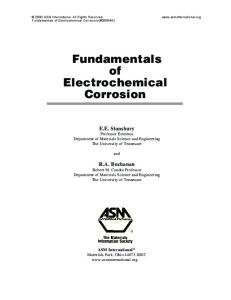
Figure 1 shows the cell room of the electrolyzer at Bayer Materials Science AG in Brunsb¨uttel, Germany. The main advantages of electrochemical processes are as follows: • Versatility: Direct or indirect oxidation and reduction, phase separation, concentration or dilution, biocide functionality, applicability to a variety of media and pollutants in gases, liquids, and solids, and treatment of small to large volumes from microliters up to millions of liters. • Energy efficiency: Lower temperature requirements than their nonelectrochemical counterparts, for example, anodic destruction of organic pollutants instead of thermal incineration; power losses caused by inhomogeneous current distribution, voltage drop, and side reactions being minimized by optimization of electrode structure and cell design. • Amenability to automation: The system inherent variables of electrochemical processes, for example, electrode potential and cell current, are particularly suitable for facilitating process automation and control. • Cost effectiveness: Cell constructions and peripheral equipment are generally simple and, if properly designed, also inexpensive. Since electrochemical reactions take place at the interface of an electronic conductor – the electrode – and an ion conductor – the electrolyte – electrochemical processes are of heterogeneous nature. This implies that, despite the advantages mentioned earlier, the performance of electrochemical processes suffers from masstransport limitations and the size of the specific electrode area. A crucial point is also the stability of cell components in
1.3 Electrochemical Reaction Engineering
.. Cell room of the hydrochloric acid electrolyzer with GDE in Brunsb uttel [28] (photo: Bayer Material Science AG). Fig. 1
contact with aggressive media, in particular, the durability and long-term stability of the electrode material and the catalysts.
1.3
Electrochemical Reaction Engineering
Electrochemical reaction engineering deals with modeling, computation, and prediction of production rates of electrochemical processes under real technical conditions in a way that technical processes can reach their optimum performance at the industrial scale. As in chemical engineering, it centers on the appropriate choice of the electrochemical reactor, its size and geometry, mode of operation, and the operation conditions. This includes calculation of performance parameters, such as space-time yield,
selectivity, degree of conversion, and energy efficiency for a given reaction in a special reactor. Electrochemical thermodynamics is the basis of electrochemical reaction engineering to estimate the driving forces and the energetics of the electrochemical reaction. Predictions of how fast the reactions may occur are answered by electrochemical kinetics. Such predictions need input from fundamental investigations of the reaction mechanism and the microkinetics at the molecular scale [29–50]. While microkinetics describes the charge transfer under idealized conditions at the laboratory scale, macrokinetics deals with the kinetics of the large-scale process for a certain cell design, taking into account the various transport phenomena. The microkinetics combined with calculations of the spatial distribution of the potential
5
6
1 Technical Scale of Electrochemistry Fig. 2 Concept of microkinetics and macrokinetics for electrochemical reactions.
Macro kinetics
Micro kinetics
Charge transfer
Reaction mechanism
Mass transport
Heat transfer
Cell design
and current density at the electrodes leads to the macrokinetic description of an electrochemical reactor [3–5, 7, 9, 10, 12–18]. The relation between micro- and macrokinetics is shown schematically in Fig. 2. The phenomenon of charge transport, which is unique to all electrochemical processes, must be considered along with mass, heat, and momentum transport. The charge transport determines the current distribution in an electrochemical cell, and has far-reaching implications on the current efficiency, space-time yield, specific energy consumption, and the scale-up of electrochemical reactors.
1.4
Fundamentals
In the following, similarities and differences in the fundamental description of chemical and electrochemical reactions are considered with a definition of symbols and signs [51, 52]. In general, a chemical reaction is written as the sum of educts Ai and products Bj � � νAi Ai = νBj Bj (1) i
j
with stoichiometric coefficients νi . The rate of the reaction is defined by 1 dnAi 1 dnBj = νAi dt νBj dt
r=
∀
i, j. (2)
where the stoichiometric coefficients are by definition negative for the educts, νAi < 0, and positive for the products, νBj > 0. Taking into account that the mole numbers of the educts are decreasing (dnAi /dt < 0) and those of the products are increasing (dnBi /dt > 0), the reaction rate r (mol sec−1 ) is always a positive number (r > 0). Electrochemical reactions are characterized by at least one electron charge transfer step taking place at the electrode/electrolyte interface. Therefore, the electron e− appears as a reactant in the reaction equation with its stoichiometric coefficient νe � i
νAi Ai + νe e− =
�
νBj Bj ,
(3)
j
Typical electrode reactions are given in Table 1. Applying Eq. (2) to the reactant e− , the reaction rate normalized to the geometrical
1.4 Fundamentals Tab. 1 Electrode reactions and standard potentials Eo [18]
Electrode reaction
Standard potential Eo /V vs SHE
Li+ + e− → Li Na+ + e− → Na Al3+ + 3e− → Al 2H2 O + 2e− → H2 + 2OH− Zn2+ + 2e− → Zn Fe2+ + 2e− → Fe Ni2+ + 2e− → Ni Pb2+ + 2e− → Pb 2H3 O+ + 2e− → H2 + 2H2 O Cu2+ + 2e− → Cu [Fe(CN)6 ]3− + e− → [Fe(CN)6 ]4− O2 + 2H3 O+ + 2e− → H2 O2 + 2H2 O Fe3+ + e− → Fe2+ Ag+ + e− → Ag O2 + 4H3 O+ + 4e− → 6H2 O Cl2 + 2e− → 2Cl− Ce4+ + e− → Ce3+ + − MnO− 4 + 8H3 O + 5e → 2+ Mn + 12H2 O O3 + 2H3 O+ + 2e− → O2 + 3H2 O F2 + 2e− → 2F−
−3.045 −2.711 −1.706 −0.8277 −0.763 −0.409 −0.230 −0.126 0 0.340 0.356 0.682 0.771 0.799 1.229 1.37 1.443 1.491
1 dne Ae νe dt
2.87
(4)
The number of moles ne transferred within a certain time t can be expressed by the electrical charge Qt = I t = Ae it and the Faraday constant F = 96 485 As mol−1 ne =
Qt F
(5)
(7)
when applied to the simplified electrode reaction νR R + νe e− = νp P with a single reactant R and product P mP =
νP MP Qt νe F
reactant R
or with respect to the
mR =
νR MR Qt νe F
(8)
Here mP and mR are the mass and MP and MR the molar mass of R and P, respectively. Owing to the sign convention of νi , the mass mR in Eq. (8) is negative, indicating that R is consumed during the reaction (Qt < 0). A prerequisite for the validity of these equations is that only the considered reaction takes place at the electrode. In reality, side reactions can occur in parallel, the individual contribution of which is given by their current efficiency �e . 1.4.1
Current Efficiency
The linear relation r=
1 dne 1 dnP = νP dt νe dt
2.07
electrode surface area Ae can be written as r=
(mol cm−2 sec−1 ) is proportional to the current density i (A cm−2 ), the sign of which is determined by the sign of the stoichiometric coefficient νe . It follows that the current density is negative (cathodic), if the electrode reaction describes a reduction process (e.g., Eq. 3), and positive (anodic) for an oxidation process (opposite direction). Equation (6) is the differential form of Faraday’s law. The common expression is obtained by integration of Eq. (2)
i , νe F
(6)
which results from (4) and (5) shows that the rate of an electrochemical reaction r
The classical definition of the current efficiency �e is based on Faraday’s law and relates the mole numbers nP of the product to that of the electron ne consumed in the
7
8
1 Technical Scale of Electrochemistry
electrochemical reaction. �eP =
mP νe F nP /νP = νP MP Qt ne /νe
(9)
In that sense, �e is the ‘‘yield of charge’’ Qt consumed in the course of the reaction. The current efficiency defined by Eq. (9) represents an average value. The differential or point current efficiency is defined by [17] 1 dnP � Ae i � �eP = νP dt νe F
(10)
which is consistent with the definition of the partial current density of the product � P , iP = i�eP . 1.4.2
Space-time Yield
Another performance criterion, which is of particular importance for the calculation of capital investment and running costs of an electrochemical reactor is the space-time ρst yield, which is the amount of product mP produced per unit of time t and reactor volume Vr ρst =
1 dmP Vr dt
νP MP e � ae i(t) νe F
id,lim = −
νe F km cR νR
(13)
This leads to the following expression: ρst = −
νP MP �e ae km cR νR
(14)
In this case, ρst is proportional to the mass-transport coefficient km , which can be increased by forced convection, for example, through agitation of the solution, enhanced electrolyte flow, turbulence promoters, or setting the electrodes in motion. Equations (12) and (14) are the key formula for the optimization of electrochemical cell design. Equation (14) is of particular importance for reactions with low concentrations, for example, recycling of metals from spent solutions or wastewater.
1.5
Electrochemical Thermodynamics
(11)
Substitution of mP from Eq. (8) leads to the point space-time yield ρst =
from charge transfer to a mass-transportcontrolled regime, where the diffusionlimited current density, as the maximum of the reaction rate, can be reached
(12)
which contains a design factor (the specific electrode area ae = Ae /Vr (cm2 /cm3 )) and a reaction factor (the product of current density and current efficiency). It is evident that optimization will be directed toward enlargement of ae and increase in the reaction rate, that is, the current density i. The latter can be achieved, for example, by shifting the reaction
The Galvani potential difference arising at the electrode/solution interface, �ϕ = ϕs − ϕe , depends specifically on the energy and density of electronic states in the two phases in contact. In principle, it is impossible to measure �ϕ at a single electrode. By combining two electrodes 1 and 2 to an electrochemical cell, the difference between the two interface potentials can be measured as the cell voltage Uc = �ϕ1 − �ϕ2 . To normalize this potential measurement, the standard hydrogen electrode (SHE) is used as a reference and the cell voltage Uc is denoted as electrode potential E versus SHE. The
1.5 Electrochemical Thermodynamics
electrode potential at equilibrium, Eo , depends on the concentrations ci or activities ai of the reactants according to the Nernst equation Eo = E o +
RT � νi ln ai νe F
(15)
i
where E o is the standard potential at ai = 1, T = 298 K, and pressure p = 1.013 × 10⁵ Pa = 1013 bar. Table 1 contains the standard potentials E o of the selected electrode reactions. The standard potentials E o versus SHE or cell voltages Uco can be calculated from thermodynamic data. The standard Gibbs free energy of the overall cell reaction �Go298 is related to the electrical work nF Uco , �Go298
= −nF
Uco
(16)
which can be gained under quasireversible operating conditions of the cell, that is, at an infinitely low reaction rate. �Go298 is the stoichiometric sum of the Gibbs free energies of formation, �Gof,i , of the reactants involved in the reaction �Go298 = Tab. 2
νi �Gof,i
o o �Go298 = �H298 − T �S298
(18)
where T �S o is the reversible heat exchanged with the environment. The entropy change �S o can be either positive or negative and is directly related to the temperature coefficient of the cell
(17)
�
∂Uco ∂T
� =− p
1 1 ∂�Go298 o = �S298 nF ∂T nF (19)
Thermodynamic data of typical reactants [41]
Reactant H2 Cl2 H3 O+ Cl− O2 H2 O Zn0 Zn++ HCl C CO
�
In (16), n is the number of electrons transferred in the overall process to maintain electroneutrality. Thermodynamic data for many chemical reactants and compounds are available as standard o and entropies S o from enthalpies �Hf,i f,i thermodynamic tables in handbooks, for example, [53, 54]. For the elements and for the proton H + (aq) in aqueous soluo values are zero by tion (H3 O+ ), the �Hf,i definition. Thermodynamic data for some typical electrochemical reactants are given in Table 2. These data are related to the Gibbs free energy of reaction �Go298 by the Gibbs–Helmholtz equation
State of aggregation g g aq aq g l s aq g s g
�Ho298 [kJmol−1 ] 0 0 0 −167.54 0 −285.25 0 −152.51 −92.53 0 −110.5
(g: gas; l: liquid; s: solid; aq: aqueous solution of activity one)
o [JK −1 mol−1 ] S298
130.74 223.09 0 55.13 205.25 70.12 41.65 −106.54 186.79 5.69 198.0
9
10
1 Technical Scale of Electrochemistry
The �Go298 values are calculated from the stoichiometric sum of the enthalpies o and the entropies S o of formation �Hf,i f,i of the species involved �Go298 =
�
o νi �Hf,i −T
i
�
o νi Sf,i
Oxygen electrode: 1 O2 + 2H+ + 2e− = H2 O with 2 o = +1.229 V versus SHE EO 2 /H2 O (21)
i
(20) If �Go298 is negative, the reaction is exergonic and should occur spontaneously, otherwise it is endergonic and does not occur or occurs in the reverse direction only. The negative sign in Eq. (16) implies that the cell voltage or standard potential of an exergonic reaction must be positive. This calls for a definition of the cell voltage measurement. According to IUPAC [51], the cell voltage is the potential difference between the right half cell I and the left half cell II, as shown in Fig. 3. The direction of the electronic current in the outer electronic circuit is defined from left to right, which means that cathodic reduction must take place in half cell I and anodic oxidation in half cell II. This is demonstrated by combining an oxygen electrode and a hydrogen electrode as the two half cells of an electrochemical cell. The half cell reactions are commonly formulated as reductions:
Hydrogen electrode: 1 o H2 with EH + /H 2 2 = 0.0 V versus SHE (22)
H+ + e− =
If the oxygen electrode is placed on the right and the hydrogen electrode on the left in Fig. 3, according to IUPAC convention, the electrode reactions must be written 1 O2 + 2H+ + 2e− = H2 O 2 H2 = 2H+ + 2e−
1 O 2 + H2 = H2 O 2
Half cell II
+
e−
e−
Half cell I
Electrochemical cell for the definition of cell voltage measurement according to the IUPAC convention [51].
Fig. 3
Oxidation
Reduction
(25)
For the example considered, the overall electron-transfer number in Eq. (16) is n = 2.
e− −
(24)
so that the sum yields the overall cell reaction and the electrons are cancelled.
Cell voltage Uc [V]
e−
(23)
1.5 Electrochemical Thermodynamics
The cell voltage under standard conditions is the potential difference between the right and left half cell: Uco = o o o − EH EO + /H = 1.229 V. Since Uc 2 /H2 O 2 is positive, the Gibbs free energy of the reaction is negative according to Eq. (16) �Go298
= −2.96485
reaction. This effect can be compensated if the cell is operated at an increased cell voltage generating the corresponding amount of Joule’s heat in the system. The corresponding cell voltage is denoted as the thermoneutral voltage 1 o with �H298 nF o o �H298 = �Go298 + T �S298 .
Uth = −
· (1.299 − 0)VAs mol−1
(27)
= −237.160 kJ mol−1 . The cell reaction (25) occurs spontaneously and the cell delivers electrical work nF Uco , which is utilized in H2 /O2 fuel cells (see also Chapter 8). Calculation of �Go298 from thermodynamic data in Table 2 yields 1 o o −�HH − �HOo 2,g ) �Go298 = (�HH 2 Ofl 2,g 2 1 o o o − SH − SO ) − T (SH 2 Ofl 2,g 2 2,g (26) �Go298 = (−285.25 − 0 − 0) − 298 1 · (70.12 − 130.74 − 205.25) 2 = −236.603 kJ mol−1 The reversible heat T �S o = −1 −48.647 kJ mol is negative. It is released by the system and cannot be exploited as electrical work. If the two half cells are arranged opposite with the hydrogen electrode on the right and the oxygen electrode on the left, the corresponding reactions are reversed and the overall process refers to the electrolysis of water with hydrogen and oxygen as the products. In this case, the cell voltage Uco is negative and �Go298 is positive. The reversible heat T �S o is positive and is taken up from the environment; the cell cools down in the course of the
It is interesting to note that, in contrast to chemical reactions, electrochemical cells can operate in principle against a positive �G if an outer current source is applied, driving the electrons in the opposite direction. This is the principle of the secondary batteries and electrochemical power sources, which can be charged and discharged to accumulate and release electrical energy. 1.5.1
Energy Yield
The costs of electrochemical processes are closely connected to the energy efficiency or energy yield, which is either related to the change of the Gibbs free energy of the reaction �G γG =
�G�e Uc,o e = � , nF Uc Uc
(28)
or to the thermal energy (enthalpy change �H ) γH =
�H �e Uth e = � . nF Uc Uc
(29)
Here Uc,o = −�G/nF is the cell voltage at equilibrium, Uc is the actual cell voltage under current operation, and Uth is the thermoneutral voltage, Eq. (27), which permits isothermal operation.
11
12
1 Technical Scale of Electrochemistry
1.5.2
the fluidized-bed cell [72–76], and the rolling tube cell [77, 78].
Specific Electrical Energy Consumption
For solid or liquid products, the specific electrical energy consumed is usually mass related Ese =
Uc νe F (J kg−1 ) νP MP �e
(30)
1.6
Electrochemical Cell Design
Different electrochemical cells have been developed for various applications in the past. According to the criteria of high mass-transport coefficient km and/or large specific electrode area ae , as predicted by Eq. (14), these cells can be classified as [20]: • Cells with relatively small electrode area but improved mass transport to increase km by setting the electrodes in motion or by applying turbulence promoters. Examples are the pump cell [55, 56], the Chemelec cell [57], the ECO cell [58–60], the beat-rod cell [61, 62], and cells with vibrating electrodes or electrolytes [63]. • Cells with enlarged electrode area in a small cell volume are found in the multiple-cathode cell [64], the Swiss-role cell [65], the extended surface electrolysis (ESE) cell [66], and the capillary gap cell [13, 67]. • Cells with three-dimensional electrodes providing enlarged specific electrode area and improved mass transport due to the specific fluid dynamics inside the threedimensional structure are, for example, the porous flow-through cell [68], the RETEC (RETEC is a trademark of ELTECH Systems Inc., Cardon, Ohio) cell [15], the packed-bed cell [69–71],
Some of them are shown, for example, in Fig. 4(a–c). The pump cell is the rotating analogue to the capillary gap cell [67]. Although this cell has not yet been employed on an industrial scale, it is interesting because of its operation principles. It consists of two static disc electrodes with current connections and a bipolar rotating disk in between. The electrolyte is pumped radially from the central tube to the outer circumference by the rotating disk. The advantage of this design is that the mass-transfer coefficient can be controlled independent of the flow rate and the residence time of the electrolyte. The Chemelec cell, Fig. 4(b), uses a fluidized bed of glass spheres as turbulence promoters to improve the mass transport to the electrodes consisting of a series of closely spaced gauze or expanded metal sheet. The residence time and the degree of conversion per pass are relatively low because the flow rate has to exceed the fluidization velocity of the bed. This cell is therefore suitable for pretreatment or recycling operations and is commonly used in the electroplating industry for maintaining a moderate metal ion concentration in a recirculated wash-water tank. High mass-transport coefficients are obtained in cells with a rotating cylinder electrode (RCE) and a small gap between the anode and the cathode, Fig. 4(a). High rates of mass transport are experienced in the turbulent flow regime, so that RCE reactors allow metal deposition at high speed, even from dilute solutions. RCE reactors have been operated at a scale involving diameters from 5 to 100 cm, with rotation speeds from 100 to 1500 rpm and currents from 1 A to 10 kA [79]. It
Fig. 4
+ − Flow + −
Multicathode cell
Waste water
(a–c) Electrochemical cell design [13].
(b)
Anolyte
− Multimesh cathode
+
Mesh electrodes
Ion-exchange membrane
Pump cell
+
Chemelec cell
Inlets
Distributor
Anolyte
−
Metal powder
− Electrolyte outlet Rod guidance Rod cathodes
Separator
+
Swiss-role cell
Electrode
Beat-rod cell
Rotation axes Electrolyte inlet
Catholyte Concentric anodes
Fluidized bed level
Electrolyte level
ECO cell
+
Rotating cylinder cathode
+ − + − + − +
Baffle plates
−
Catholyte
Magnetically driven rotor running on ceramic shaft
Stator
Rotor
DSA mesh anode
(a)
Flow
+ Current connections −
Flow
Anolyte
1.6 Electrochemical Cell Design 13
Fig. 4
(Continued).
(c)
Inlet
Packed-bed cathode
Packed-bed enViro cell
Overflow channel
Catholyte outlet
Flow distributor
Large particle outlet
Graphite anode Fluidizedbed cathode
Outlet
Small particle inlet +
Anode
Anolyte
Fluidized-bed cell
Catholyte
Cathode − feeder electrode
Ion-exchange membrane
Gas outlet
Inner cylinder anode
Outer plate anodes
Rotation axes
Membrane
Anolyte outlet + −
Rolling tube cell
Rolling particles (graphite)
Rotating sieve tube
Tankhouse
Cathodic feeder electrode
14
1 Technical Scale of Electrochemistry
1.6 Electrochemical Cell Design
is possible to design RCE reactors with a scrapping device to remove deposited metal powder continuously from the cathode surface. The so-called ECO cell, Fig. 4(a), with a cascade of baffle plates around the rotating cylinder cathode, which prevent back mixing of the solution to a great extent, attains high degrees of conversion. A cell with a special design is the beatrod cell, Fig. 4(a), which was mainly used in small electroplating shops. Supported cathode rods slowly rotate within an annular type of chamber in the electrolysis tank. The rods strike one another so that the metal deposit is removed and settles as a powder at the bottom. An efficient way of fitting large planar electrodes in a small volume is the design of the Swiss-role cell, Fig. 4(b). Thin metal foils are separated by a plastic mesh and wrapped around a central core. The ohmic drop within the thin metal foil is largely compensated by contacting the foils on the opposite side. The electrolyte flows axially through the electrode pack. Large space-time yields are realized and masstransport conditions are favorable since the separator also functions as a turbulence promoter. Mesh electrodes wrapped around a perforated winding core lead to another version of the Swiss-role cell with radial flow. Cells with mesh electrodes instead of foils are known as extended surface electrode ESE cells. A commercial system of this type is the RETEC cell, which contains 6–50 three-dimensional cathodes as flow-through metal sponge electrodes [15]. The cell is used in closed water recycling systems in the electroplating industry with applications similar to those of the Chemelec cell, Fig. 4(b). A simple three-dimensional electrode is obtained by using a packed bed of conductive particulate material through which the
electrolyte is pumped. Numerous versions of packed-bed cells have been described in the literature [13, 68, 80–84]. The potential distribution and optimum bed depth for metal deposition, Mez+ + ze− = Me, was calculated as a function of the effective particle and solution conductivities (κp , κs ) [13, 20]. For rectangular cell geometry and fully developed diffusion limited current density within the particle bed, the following relation was found for the optimal bed depth: � 2εκs �η hopt = ae zF km cMez+ (condition κp � κs )
(31)
where ε is the voidage of the 3-D electrode structure and �η the overvoltage range of the prevailing limiting diffusion current density in the microkinetic polarization curve. According to Eq. (31), the optimal bed depth increases with decreasing metal ion concentration by an inverse square root dependence. This has led to the enVirocell design depicted in Fig. 4(c), where the bed depth widens with decreasing concentration along the flow direction of the solution. The principle of fluidized-bed electrolysis originates from Fleischmann and Goodridge [73]. It has been examined for different applications [72, 85, 86] and was applied on an industrial scale for metal recovery [75, 76]. The electrolyte flows from bottom to top through a bed of fluidized particles, which are charged via a feeder electrode. The advantage is that the particles are held in suspension, thus avoiding bed blockage by the deposited metal. Because the height of the cell is restricted to about 2 m for hydraulic reasons and the fluidization velocity has to be maintained at a relatively high level, short residence times and thus only a limited degree of
15
1 Technical Scale of Electrochemistry
conversion per pass can be achieved. Continuous operation with recirculation of the solution and cascade arrangement of cells has therefore been used in practical applications. Moving and circulating bed electrodes, also denoted as a spouted bed, are described in the literature [87]. As an example, the rolling tube cell is shown in Fig. 4(c) [77, 78]. In principle, this cell resembles the wellknown plating process for piece goods, using slowly rotating barrels. The rotating drum is only partially filled with particles to achieve thorough agitation. This cell has proved to be especially useful for silver and gold recovery. Further developments of moving bed electrodes and their application can be found elsewhere [88]. In Fig. 5, the specific electrode area ae (cm−1 ) of various electrochemical cells is shown as a function of a characteristic length (interelectrode distance or particle diameter). It can be seen that the electrochemical cells differ significantly in their specific area and characteristic length by orders of magnitude. At a current
efficiency of �e = 1, the space-time yield is mainly determined by the product ae i =
I = j ∗. Vr
(32)
The quantity j ∗ (A cm−3 ) can be considered as a volumetric current density or a current concentration, also shown in Fig. 5 as a function of the characteristic length. Extremely high current densities, for example, 10 kA cm−2 in the chloralkali electrolysis, can be applied only in a limited number of cases, the number of cells with high specific electrode area is restricted to cases of low current densities [13]. A special cell concept combining ease of construction and scale-up is the capillary gap cell, which is mainly applied in electro-organic synthesis, where low conductivities of the electrolytes are a major problem, Figs 6 and 7, [13, 28, 67, 89]. The cell consists of circular disk electrodes with a small interelectrode gap (1–2 mm) to minimize the ohmic voltage drop in the electrolyte. The electrolyte
Porous flowthrough cell
100
Porous flowthrough cell
100
Fluidizedbed cell 10
Current concentration j * [A cm−3]
Plate-andframe cell Specific electrode area ae [cm−1]
16
Packed-bed cell
Swiss-roll cell
1.0
Plate-andframe cell
0.10
Swiss-roll cell
Packed-bed cell 0.01
Chloralkali cell (mercury process) 0.1 00.1
0.1
Chloralkali cell (mercury process)
Fluidizedbed cell 1
Characteristic length [cm]
10
0.001 00.1
0.1
1
Characteristic length [cm]
Specific electrode area ae and volumetric current concentration j∗ as a function of the characteristic length of different electrochemical cells [13].
Fig. 5
10
1.6 Electrochemical Cell Design Current collector Cell hood Outlet Contact plate graphite Product + H2 Graphite disks “Capillary gap”(1–2 mm) Electrolyte flow Base plate/connector Inlet Fig. 6
Fig. 7
Scheme of the capillary gap cell of BASF AG [28].
Cell room with capillary gap electrolyzers [28] (photo: BASF AG).
enters via a central channel and is radially distributed between the circular disk electrodes. In the bipolar configuration, the disks are isolated from each other and connected at the end plates to the voltage supply. To avoid reconversion of the product at the counterelectrodes in the undivided cells, the disk geometry and flow velocity must be carefully tuned to ensure that the diffusion layer thickness,
which increases along the radius, does not reach the counterelectrode. Although the scale-up of the stack height and number of disks is simple, the outer disk radius cannot be enlarged. A number of electroorganic processes with methoxylation reactions for production of, for example, anisaldehyde and tert-butylbenzaldehyde, were recently developed at BASF [90, 91] using a somewhat modified cell with
17
18
1 Technical Scale of Electrochemistry
graphite felt electrodes. They were also successful in developing ‘‘paired electrolysis’’ with the simultaneous formation of valuable products at the anode and at the cathode. A methoxylation at the anode was combined, for example, with the reduction of phthalic acid dimethylester to phthalide, a valuable precursor in pest management chemistry [92]. Anode :R-C6 H4 -CH3 −4e− +2 CH3 OH −−−→ R-C6 H4 -CH(OCH3 )2 + 4 H+ Cathode :C6 H4 (COOCH3 )2 +4e− +4 H+ −−−→ C8 H8 O2 + 2 MeOH Another cell design strictly directed toward minimization of the ohmic drop in the electrolyte, especially if gases are developed at the electrodes, is the zerogap cell, shown in Fig. 8 [17, 93, 94]. The perforated electrodes are pressed directly onto the diaphragm by the current collectors providing optimum contact across the whole electrode area. However, uneven
current distribution and voltage drop in the electrolyte as well as in the diaphragm cannot be avoided, as illustrated in Fig. 8. Zero-gap cells have been successfully used for alkaline water electrolysis [93, 94]. Another design that is used in chloralkali electrolysis, water electrolysis, and electro-organic synthesis [95–97] is the solid polymer electrolyte (SPE) cell, where an ion exchanger membrane, for example, Nafion, serves as the electrolyte, Fig. 9. The microporous catalytic reaction layers are pressed directly onto the membrane with porous current collectors allowing transport of dissolved reactants and gaseous products into and out of the reaction layer. The advantages of SPE technology are as follows: electro-organic synthesis without an additional supporting electrolyte, reduced energy demand for separation and recycling processes, and elimination of side reactions with the electrolyte at moderate reaction conditions with ease of process control. The structure of the SPE electrolysis cell is similar to that of the membrane
Electrodes
Schematic distribution of current lines
Gas bubbles
Diaphragm
Fig. 8 Gas evolution and current distribution at perforated zero-gap electrodes [13].
1.6 Electrochemical Cell Design Solid polymer electrolyte (SPE) cell with cation exchanger Anode with catalyst layer membrane Nafion [13].
Fig. 9
Cathode with catalyst layer Metal mesh
Bipolar plate
Nafion 120 Anodic current collector
electrode assembly in polymer electrolyte membrane (PEM) fuel cell technology, which is described in detail in Chapter 8. References 1. C. Wagner, The scope of electrochemical engineering in Advances in Electrochemistry and Electrochemical Engineering (Eds.: P. Delahaye, C. W. Tobias), WileyInterscience, New York, London, Sydney, 1962, p. 1, Vol. 2. 2. C. L. Mantel, Electrochemical Engineering, 4th ed., MacGraw-Hill, New York, 1960. 3. O. Levenspiel, Chemical Reaction Engineering, 2nd ed., wiley, New York, 1972. 4. J. S. Newman, Electrochemical Systems, Prentice-Hall, Englewood Cliffs, 1973. 5. D. J. Pickett, Electrochemical Reactor Design, 2nd ed., Elsevier, Amsterdam, 1979. 6. F. Beck, Elektroorganische Chemie, VCH, Weinheim, 1974. 7. J. O. M. Bockris, B. E. Conway, E. Yeager, Comprehensive Treatise of Electrochemistry, Plenum Press, New York, Vol. 2, Electrochemical Processing, 1981, Vol. 3, Electrochemical Energy Conversion and Storage, 1981, Vol. 4, Electrochemical Material Science, 1981, Vol. 6, Electronics: Transport, 1983. 8. F. Coeuret, A. Storck, Elements de Genie Electrochimique, Tecdoc, Paris, 1984.
Cathodic current collector
9. F. Hine, Electrode Processes and Electrochemical Engineering, Plenum Press, New York, 1985. 10. T. Z. Fahidy, Principles of Electrochemical Reactor Analysis, Elsevier, Amsterdam, 1985. 11. I. Rouzar, K. Micka, A. Kimla, Electrochemical Engineering, Elsevier, Amsterdam, 1986, Vol. 1 and 2. 12. E. Heitz, G. Kreysa, Principles of Electrochemical Engineering, VCH, Weinheim, 1986. 13. F. Beck, H. Goldacker, G. Kreysa et al., Electrochemistry in Ullmann’s Encyclopedia of Industrial Chemistry, VCH, Weinheim, 1987, pp. 183–254, Vol. A9. 14. K. Scott, Electrochemical Reaction Engineering, Academic Press, London, 1991. 15. D. Pletcher, F. C. Walsh, Industrial Electrochemistry, Chapman and Hall, London, 1993. 16. F. Goodridge, K. Scott, Electrochemical Process Engineering, Plenum Press, New York, 1995. 17. H. Wendt, G. Kreysa, Electrochemical Engineering, Springer, Berlin, 1999. 18. V. M. Schmidt, Elektrochemische Verfahrenstechnik, Wiley-VCH, Weinheim, 2003. 19. J. O. M. Bockris, Electrochemistry of Cleaner Environments, Plenum, New York, 1972. 20. G. Kreysa, Reactor design for electrochemical water treatment in Process Technologies for Water Treatment (Ed.: S. Stucki), Plenum Publishing Corporation, New York, 1988. 21. D. Pletcher, N. L. Weinberg, The Green Potential of Electrochemistry, Chemical
19
20
1 Technical Scale of Electrochemistry
22. 23. 24.
25.
26. 27.
28. 29. 30. 31. 32. 33.
34.
35.
36. 37.
38.
39. 40.
41.
Engineering (London), 1992, Aug. 98–103 (Part 1), Nov. 132–141 (Part 2). K. Rajeshwar, J. G. Ibanez, G. M. Swain, J. Appl. Electrochem. 1994, 24, 1077. C. A. C. Sequeira, Environmentally Oriented Electrochemistry, Elsevier, Amsterdam, 1994. S. Trasatti, Electrochemistry and the environment: the role of electrocatalysis, Int. J. Hydrogen Energy 1995, 20, 835. K. Rajeshwar, J. G. Ibanez, Fundamentals and Application in Pollution Abatement, Academic Press, San Diego, 1997. D. Simonson, Electrochemistry for a cleaner environment, Chem. Soc. Rev. 1997, 26, 181. K. J¨uttner, U. Galla, H. Schmieder, Electrochemical approaches to environmental problems in the process industry, Electrochim. Acta 2000, 45, 2575. D. Hoormann, J. J¨orissen, H. P¨utter, Chem.Ing.-Tech. 2005, 77, 1363–1376. P. Delahay, Double Layer and Electrode Kinetics, Wiley Interscience, New York, 1965. K. J. Vetter, Electrochemical Kinetics, Academic Press, New York, 1967. P. W. Atkins, Physical Chemistry, 3rd ed., Oxford University Press, Oxford, 1986. J. Koryta, J. Dvorak, Principles of Electrochemistry, Wiley, Chichester, 1987. D. D. Macdonald, Transient Techniques in Electrochemistry, Plenum Press, New York, 1977. J. Lipkowsky, P. Ross, Frontiers of Electrochemistry, Wiley, New York, Vol. 1: Adsorption of Molecules at Metal Electrodes, 1992, Vol. 2: Structure of Electrified Interfaces, 1993. C. M. A. Brett, A. M. O. Brett, Electrochemistry, Principles, Methods and Applications, Oxford University Press, Oxford, 1993. E. Gileadi, J. Wang, Electrode Kinetics, Wiley, New York, 1994. K. B. Oldham, J. C. Myland, Fundamentals of Electrochemical Science, Academic Press, San Diego, CA, 1994. A. Mozik, W. Schmickler, F. Willig, Surface Electron Transfer Processes, VCH, Weinheim, 1995. W. Schmickler, Interfacial Electrochemistry, Oxford University Press, Oxford, 1996. E. B. Budevski, G. T. Staikov, W. J. Lorenz, Electrochemical Phase Formation and Growth, Wiley, New York, 1996. A. Hamnett, C. H. Hamann, W. Vielstich, Electrochemistry, VCH, Weinheim, 1997.
42. J. O. M. Bockris, A. K. N. Reddy, M. GamboaAldeco, Modern Electrochemistry 2A – Fundamentals of Electronics, Kluwer, New York, 1998. 43. M. Paunovic, Fundamentals in Electrochemical Deposition, Wiley, New York, 1998. 44. W. J. Lorenz, W. Plieth, Electrochemical Nanotechnology, Wiley-VCH, Weinheim, 1998. 45. J. Grimshaw, Electrochemical Reactions and Mechanisms in Organic Chemistry, Elsevier, Amsterdam, 2000. 46. R. Memming, Semiconductor Electrochemistry, Wiley-VCH, Weinheim, 2000. 47. J. Bard, L. R. Faulkner, Electrochemical Methods, 2nd ed., Wiley, New York, 2001. 48. J. W. Schultze, G. Staikov, Scaling Down in Electrochemistry: Electrochemical Micro- and Nanosystem Technology, Elsevier, Amsterdam, 2001. 49. H. Kaesche, Corrosion of Metals, Physicochemical Principles and Current Problems, Springer, Berlin, 2003. 50. H. H. Girault, Analytical and Physical Electrochemistry, EPFI Press, Marcel Dekker, 2004. 51. International Union of Pure and Applied Chemistry: Gr¨oßen, Einheiten und Symbole in der Physikalischen Chemie (Ed.: K.-H. Homann), VCH, Weinheim, 1996. 52. G. Gritzner, G. Kreysa, Nomenclature, symbols and definitions in electrochemical engineering, J. Electroanal. Chem. 1993, 360, 351. 53. Handbook of Chemistry and Physics, Robert and Weast, 1977. 54. I. Barin, O. Knacke, O. Kubaschewski, Thermodynamical Properties of Inorganic Substances, Springer, Berlin, 1973. 55. R. E. W. Janson, R. J. Marshall, Chem. Eng. 1976, 315, 769. 56. R. E. W. Janson, N. R. Tomov, Chem. Eng. 1977, 327, 867. 57. C. L. Lopez-Cacicedo, Inst. Chem. Eng. Symp. Ser. 1975, 42, 29. 58. D. R. Gabe, J. Appl. Electrochem. 1974, 4, 91. 59. F. S. Holland, Chem. Ind. (London), 1978, 13, 453. 60. L. J. Ricci, Chem. Eng. 1975, 82(27), 29. 61. R. Kammel, H.-W. Lieber, Galvanotechnik 1977, 68, 710. 62. W. G¨otzelmann, Galvanotechnik 1977, 68, 789. 63. D. Bruhn, W. Dietz, K.-J. M¨uller, C. Reynvaan, EPA 86109265.8, 1986.
1.6 Electrochemical Cell Design 64. A. Storck, P. M. Robertson, N. Ibl, Electrochim. Acta 1979, 24, 373. 65. P. M. Robertson, F. Schwager, N. Ibl, J. Electroanal. Chem. 1975, 65, 883. 66. K. B. Keating, J. M. Williams, Res. Rec. Conserv. 1976, 2, 39. 67. F. Beck, H. Guthke, Chem.-Ing.-Tech. 1969, 41, 943. 68. D. N. Bennion, J. Newman, J. Appl. Electrochem. 1972, 2, 113. 69. G. Kreysa, Chem.-Ing.-Tech. 1983, 55, 23. 70. G. Kreysa, C. Reynvaan, J. Appl. Electrochem. 1982, 12, 241. 71. G. Kreysa, Elektrochem. Zelle, DE 26 22 497, 1976. 72. J. R. Backhurst, J. M. Coulson, F. Goodridge, et al., J. Electrochem. Soc. 1969, 116, 1600. 73. J. R. Backhurst, M. Fleischmann, F. Goodridge, R. E. Plimley, GB Pat, 1 194 181, 1970. 74. H. Scharf, DE 22 27 084, 1972. 75. C. Raats, H. Boon, W. Eveleens, Erzmetall 1977, 30, 365. 76. G. van der Heiden, C. Raats, H. Boon, Chem. Ind. (London), 1978, 13, 465. 77. R. Kammel, H.-W. Lieber, Galvanotechnik 1978, 69, 687. 78. W. G¨otzelmann, Galvanotechnik 1979, 70, 596. 79. D. R. Gabe, F. C. Walsh, Trans. IchemE 1990, 68B, 107. 80. G. Kreysa, Chem.-Ing.-Tech. 1978, 50, 332. 81. G. Kreysa, Metalloberf¨ache 1980, 34, 494. 82. G. A. Carlson, E. E. Estep, D. Jacqueau, Chem.-Ing.-Tech. 1973, 45, 217. 83. R. S. Wenger, D. N. Bennion, J. Appl. Electrochem. 1976, 6, 385.
84. J. van Zee, J. Newman, J. Electrochem. Soc. 1977, 124, 706. 85. D. S. Flett, Chem. Ind. (London), 1971, 10, 300. 86. D. S. Flett, Chem. Ind. (London), 1972, 14, 983. 87. K. Scott, J. Appl. Electrochem. 1988, 18, 504. 88. H. Bergmann, H. Hertwig, F. Nieber, Chem. Eng. Proc. 1992, 31, 195. 89. J. J¨orissen, Practical Aspects of Preparative Scale Electrochemistry, Encyclopedia of Electrochemistry, Organic Electrochemistry (Ed.: H. Sch¨afer), Viley-VCH, Weinheim, 2004, Vol 8, Chapter 2. 90. H. P¨utter, Industrial electroorganic chemistry in Hrsg., Organic Electrochemistry (Eds.: H. Lund, O. Hammerich), 4th ed., Marcel Dekker, New York, 2001, pp. 1259. 91. N. Aust, A. Fischer, T. Freund, U. Griesbach, G. Heyderich, H. P¨utter, D. Z¨ollinger, New electrochemical oxidations – green and sustainable chemistry for valuable intermediates, ISE 55th Annual Meeting, Thessaloniki, 2004. 92. H. Hannebaum, H. P¨utter, Chemie in unserer Zeit 1999, 33, 373–374. 93. J. Fischer, H. Hofmann, G. Luft, et al., AIChE J. 1980, 26, 794. 94. J. Divisek, H. Schmitz, J. Mergel, Chem.Ing.-Tech. 1980, 52, 465. 95. S. Stucki, A. Menth, Ber. Bunsen-Ges. Phys. Chem. 1980, 84, 1008. 96. J. J¨orissen, Electrochim. Acta 1996, 41, 553–562. 97. J. J¨orissen, J. Appl. Electrochem. 2003, 33, 969–977.
21
23
2
Electrocatalysis A. Katsaounis, S. Brosda, and C.G. Vayenas University of Patras, Patras, Greece
2.1
Introduction . . . . . . . . . . . . . . . . . . . . . . . . . . . . . . . . . . . . . .
25
2.2
Adsorption . . . . . . . . . . . . . . . . . . . . . . . . . . . . . . . . . . . . . . .
28
2.3 2.3.1 2.3.2 2.3.3 2.3.4 2.3.5
Basic Electrokinetic Principles and Experimental Techniques Electrokinetic and Mass-transport Control . . . . . . . . . . . . . The Measurement of IR-free Electrocatalyst Overpotential . . Cyclic Voltammetry . . . . . . . . . . . . . . . . . . . . . . . . . . . . AC-impedance Spectroscopy . . . . . . . . . . . . . . . . . . . . . . Normalization of Active Surface . . . . . . . . . . . . . . . . . . . .
. . . . . .
. . . . . .
. . . . . .
. . . . . .
. . . . . .
34 34 36 38 43 47
2.4 2.4.1 2.4.2 2.4.3 2.4.4 2.4.5
Theory of Electrocatalysis . . . . . . . . . . . . . . . Overpotentials and the Butler–Volmer Equation Volcano Plots . . . . . . . . . . . . . . . . . . . . . . . Transition State Approaches . . . . . . . . . . . . . Quantum Mechanics–based Models . . . . . . . . Promotional Effects . . . . . . . . . . . . . . . . . . .
. . . . . .
. . . . . .
. . . . . .
. . . . . .
. . . . . .
48 48 51 53 54 57
2.5
The Hydrogen Oxidation/Evolution Reaction . . . . . . . . . . . . . . . .
58
2.6
Oxygen Reduction/Evolution Reaction . . . . . . . . . . . . . . . . . . . . .
60
2.7
Oxidation of Small Organic Molecules . . . . . . . . . . . . . . . . . . . . .
63
2.8
Other Important Electrocatalytic Systems . . . . . . . . . . . . . . . . . . .
66
2.9
Electrochemical Promotion of Catalytic Reactions . . . . . . . . . . . . .
69
2.10
Promotional Rules in Catalytic and Electrocatalytic Systems . . . . . .
76
. . . . . .
. . . . . .
. . . . . .
. . . . . .
. . . . . .
. . . . . .
. . . . . .
. . . . . .
. . . . . .
Encyclopedia of Electrochemistry. Edited by A.J. Bard and M. Stratmann Vol. 5 Electrochemical Engineering. Edited by Digby D. Macdonald and Patrik Schmuki Copyright 2007 Wiley-VCH Verlag GmbH & Co. KGaA, Weinheim. ISBN: 978-3-527-30397-7
24
2 Electrocatalysis
2.11
Concluding Remarks . . . . . . . . . . . . . . . . . . . . . . . . . . . . . . . . References . . . . . . . . . . . . . . . . . . . . . . . . . . . . . . . . . . . . . . .
80 80
25
2.1
Introduction
The term electrocatalysis was first introduced by Grubb in 1963 [1] in connection with the anodic and cathodic chargetransfer reactions in fuel cells. However, the first systematic experimental investigations of various electrocatalysts had been carried out in the 1920s by Bowden and Rideal [2] and the concept and first interpretation of electrocatalysis had been introduced in the 1930s by Horiuti and Polanyi [3]. Their theory and its extensions and improvements have been analyzed lucidly by Bockris [4–6]. Recent reviews of progress in electrocatalysis can be found in more general [6–8] or specialized books [9–11]. An electrocatalyst is an electrode that can accelerate the approach to equilibrium of an electrochemical process, which involves a net charge transfer, without itself being consumed in the process. This definition is in analogy to that of a catalyst which is a substance (quite often a solid) which can accelerate, without being consumed, the approach to equilibrium of a chemical process in a gaseous or liquid mixture. In heterogeneous catalysis, the specific activity of a catalyst is usually expressed as turnover frequency (TOF) (s−1 )
which expresses the number of catalytic turnovers per surface catalyst atom per second. Typical turnover frequencies of industrial catalytic processes are 10−3 to 102 s−1 . Slower TOFs are economically uninteresting and larger ones are usually not realizable in a practical environment because of diffusional limitations. In electrocatalysis, the activity of different electrocatalysts is usually expressed via the exchange current Io , and the specific activity, via the exchange current density, io (A cm−2 ), still often computed on the basis of the superficial electrode surface area. Only when the current is normalized using the true surface area of the electrode–electrolyte interface, the comparison between different electrocatalysts is truly meaningful. The determination of the true surface area of porous electrodes is discussed in Sect. 2.3.5. For a Pt(111) surface, with a surface density of 1.5 × 10¹⁵ atoms cm−2 , the current density corresponding to a TOF of 1 s−1 is 0.18 mA cm−2 for a oneelectron charge-transfer process. Such exchange current densities based on the real electrocatalyst surface area are quite typical for a decent electrocatalyst for H2 evolution or oxidation. Thus, one may conclude that the order of magnitude of the TOFs of catalytic and electrocatalytic reactions are quite similar. In the latter
Encyclopedia of Electrochemistry. Edited by A.J. Bard and M. Stratmann Vol. 5 Electrochemical Engineering. Edited by Digby D. Macdonald and Patrik Schmuki Copyright 2007 Wiley-VCH Verlag GmbH & Co. KGaA, Weinheim. ISBN: 978-3-527-30397-7
2 Electrocatalysis
case, of course, the TOF can be very significantly modified by the electrode potential. Different electrodes can have dramatically different electrocatalytic activity. An example is given in Fig. 1 which shows current–potential curves obtained with different electrodes for the same chargetransfer reaction, that is, H2 evolution. One observes that at the same overpotential, the current density, i, obtained with different electrocatalysts and, thus, also the specific rate of H2 evolution i/F , where F is the Faraday constant (96 450 C mol−1 ), varies by many orders of magnitude. In this figure, the current has been normalized using the superficial electrode surface area and this is the main reason for the very large differences that are observed between ‘‘bright’’ Pt and ‘‘spongy’’ Pt (Fig. 1). Horiuti and Polanyi [3] were the first to provide an interpretation of electrocatalysis (Fig. 2). The potential energy of a proton moving toward the electrode exhibits a maximum at the intersection of the potential energy curve of the proton in solution and that of a H atom adsorbed on the electrode. A good electrocatalyst is that Potential against saturated calomel electrode
26
in which this maximum is small. Upon varying the electrode potential, the energy of adsorption varies by ��Hads and thus the activation barrier changes by β��Hads where the parameter β (typically of the order of 0.5–1) dictates, to a large extent, the slope of the Tafel diagrams of Fig. 1. Although, during the last 50 years, significantly more detailed classical or quantum mechanical treatments have been formulated to describe and predict the classical Tafel behavior of electrocatalysis (Fig. 1) [12–22], the basic ideas of the Horiuti and Polanyi interpretation remain fruitful. In fact, the linear variation in adsorption enthalpies with potential is well established in high-temperature solid electrolyte electrochemistry [23, 24] (Fig. 3), where enthalpies and entropies of adsorption are quite straightforward to measure using standard surface science techniques, such as temperature-programmed desorption (TPD). This is similar with the observed linear variation of the adsorption enthalpies of alkalis on metal surfaces with the adsorption-induced change in catalyst work function [23, 25] (Fig. 4). It is worth noting in Figs 3 and 4 that the slope of the
−1.4 −1.2
I
Fig. 1 Some of the first published comparative current–potential (Tafel) plots obtained by Bowden and Rideal [2, 4]. I. Mercury. II. Platinized VI V III −0.8 mercury, 1/100 covered. III. Platinized IV mercury, thin film of Pt. IV. Etched −0.6 VII silver, new. V. Etched silver, old. VI. VIII Polished silver. VII. Bright platinum. −0.4 VIII. Spongy platinum. (In Curve VIII the current density is expressed in amperes −0.2 ×10⁻⁶ in order to bring it on the figure. 0 It should be displaced two divisions to 0 0.5 1 1.5 2 2.5 3 3.5 4 4.5 the right.) (Reprinted with permission Logarithm of apparent current density from Ref. 2, Copyright 1928 by The Royal −2 −7 [A cm × 10 ] Society).
−1
II
2.1 Introduction The effect of the variation of the ��H on the potential energy–distance diagram. (Reprinted with permission from Ref. 4, Copyright 1994 by Elsevier).
Fig. 2
PE
C
A B ∆HAox ∆∆H
∆HBox
∆∆H ox = b∆∆HAds
XAB
Effect of catalyst potential on the oxygen desorption activation energy, Ed , calculated from the Redhead analysis of O2 TPD spectra for Pt, Ag, and Au electrodes deposited on YSZ. (Reprinted with permission from Ref. 24, Copyright 1997 by Springer). Fig. 3
∆Φ [eV] 3
Ed [eV]
2.5 Au 2 Pt 1.5 Ag 0
0.2
0.4
0.6 0.8 eU*WR [eV]
1
3.5
80
3
70 60
2.5
50 2
1
40
Na K STD K Cs STD
1.5
−4
−3
−2 ∆Φ [eV]
−1
30 0
1.2
Ed [kcd mol−1]
Fig. 4 Effect of work function change �� on the alkali desorption energy [23, 25]. (Reprinted with permission from [25], Copyright 1987 by Elsevier).
Ed [eV]
1
27
28
2 Electrocatalysis
straight lines are of the order −1 for atomic oxygen and +1 for atomic potassium, an observation supported by rigorous quantum mechanical cluster treatments [23, 26]. This linear variation in adsorption enthalpies with potential is also responsible for the effect of electrochemical promotion on non-Faradaic electrochemical modification of catalytic activity (NEMCA) effect where electrocatalysis is used to generate promoters for catalytic (no net charge transfer) reactions in situ. It has been shown [26] that, in most cases, these linear on near-linear variations in adsorption enthalpies with potential reflect the fact that adsorption involves formation of a chemical (chemisorptive) bond, between the adsorbate and the electrode, in the presence of a very strong electric field (typically 1010 V m−1 or 1 V A˚ −1 ) created in the double layer formed at the electrode–liquid or electrode–gas interface owing to the presence of the adsorbate and other weakly or strongly coadsorbed species. This electric field varies linearly with potential (it vanishes at the potential of zero charge, pzc) [23, 27] and its interaction with the adsorbate dipoles is the main cause for the observed linear variation in adsorption enthalpies with potential. During the last 15 years, the urgent need for developing practical fuel cell devices has led to an unprecedented interest in electrocatalysis for the development of efficient anodes and cathodes both in aqueous [9] and in high-temperature [28] electrochemistry.
2.2
Adsorption
The role of adsorption in electrocatalysis is as important as it is in heterogeneous catalysis. In aqueous electrochemistry, the
presence of H2 O makes the study of adsorption more complex than in solidstate electrochemistry or in heterogeneous catalysis. The basic principles of the subject are analyzed lucidly by Gileadi [29]. The simplest isotherm in electrocatalysis is the electrochemical Langmuir isotherm. Considering, for example, the adsorption of chlorine atoms on a metal electrode, M, one can write: � Cl− + M − M � − − Cl + e
(1)
and the electrochemical Langmuir isotherm is θ/(1 − θ) = Kc exp[F U/RT ]
(2)
where θ is the coverage of Cl on the metal surface, U is the electrode potential, c is the concentration of Cl− ions in the solution, and K is an adsorption equilibrium constant. If the adsorption is dissociative, for example + − − � 2H 2M + H2 � − + 2e + 2M
− � 2M � − −H
(3)
then the Langmuir isotherm can be expressed as θ 2 /(1 − θ)2 = KpH2 = Kc2 exp[−F U/RT ] (4) where c is the proton concentration. If the adsorption involves a large molecule which occupies n sites on the surface, then Eq. (2) can be written in the form θ/(1 − θ)n = Kc exp[F U/RT ]
(5)
where the sign of the potential in (5), as well as in Eqs (2) and (4), is dictated by whether an electron is taken from or given to the electrocatalyst during the adsorption
2.2 Adsorption Electrochemical Langmuir isotherm. Plots of fractional coverage θ versus (a) concentration and (b) potential or log c, for three values of the equilibrium constant K = 1, 5, and 25. (Reprinted with permission from Ref. 29, Copyright 1993 by Wiley-VCH).
Fig. 5
1 K 25
Fractional coverge [θ]
0.8
5 0.6
0.4
1
0.2
0
0
0.4
0.8
(a)
0 1
0.8 Fractional coverge [θ]
1.2
1.6
2
C [mM] U vs arbitary reference [mV] 60 120 180 240
K
25
5
300
1
0.6
0.4
0.2
0 −3 (b)
process. Thus, the sign is positive when the adsorbate starts as an anion and negative when the adsorbate starts as a cation. Figure 5 shows plots of Eq. (2) for various values of K. In Fig. 5(a), the coverage θ is plotted versus c, while in Fig. 5(b) it is plotted versus log c. In the latter case, increasing K causes a parallel shift in the θ versus log c plot. A change in the potential equal to 2.3RT/F has the same effect on θ as a change of a factor of 10 in the ion concentration.
−2
−1
0
1
2
log C [mM]
The assumptions of the electrochemical Langmuir isotherm are the same as those for the Langmuir isotherm in heterogeneous catalysis, that is, surface homogeneity and negligible lateral adsorbate interactions. This leads to a K value which does not depend on θ and, thus, to a standard free energy of adsorption, �G◦ , which also does not depend on θ. Note that in the context of the Langmuir or electrochemical Langmuir adsorption isotherm the standard state of the adsorbate is at θ = 1/2.
29
2 Electrocatalysis
The first refinement of the electrochemical Langmuir isotherm is the Frumkin isotherm, which is obtained by assuming a linear dependence of �G◦ on θ, that is, ◦
◦
�G = �Go + rθ
(6)
where the parameter r (typically |r| = 20–100 kJ mol−1 ) is a measure of the surface heterogeneity and, usually more importantly, a measure of the strength of lateral adsorbate–adsorbate interactions, which can be mediated either via the aqueous or gas phase or via the metal electrode itself. A positive r implies repulsive adsorbate–adsorbate interactions and a negative r implies attractive adsorbate interactions. The resulting isotherm θ/(1 − θ) exp(rθ/RT ) = Ko c exp(F U/RT )
(7)
is known as the Frumkin isotherm. Figure 6 shows the dependence of θ on potential for a fixed value of c. The plots of θ versus c at fixed potential are qualitatively similar. For r/RT < −4, one obtains steady-state multiplicity, that is, for fixed c there are three steady-state coverage values, two of which (the lowest
and the highest) are stable, and usually very different. The high-coverage state corresponds to surface ‘‘condensation’’, or island formation, due to the attractive lateral interactions which lead to an ordered two-dimensional adsorbate surface structure. The Frumkin isotherm is mathematically equivalent to the effective doublelayer (EDL) isotherm recently introduced in heterogeneous catalysis [23, 27] and which accounts for the existence of an overall neutral double layer at the metal–gas interface. This type of isotherm is very useful in describing the effect of electrochemical promotion of catalysis (EPOC or NEMCA effect), which is further discussed in the following text, and refers to the pronounced and strongly non-Faradaic change in catalytic activity observed upon electrochemical supply or removal of ions to or from a catalyst surface. This effect has been studied in much more detail in solid-state electrochemistry, utilizing Y2 O3 -stabilized ZrO2 (YSZ), (an O2− conductor) or β �� -Al2 O3 (a Na+ conductor) [23], than in aqueous systems [23, 30, 31], where, on the other hand, the NEMCA effect was recently shown to play
1 −8
Fractional coverage [θ]
30
−4
0
8
16
r f =_ RT 0.1
0.01
0.001 −200
−100
0
100
f [V]
200
300
Fig. 6 Frumkin isotherm, plotted as log θ versus U, for different values of f = r/RT. Negative values of f correspond to a lateral attraction interaction (i.e., to an increase of |�G◦θ | with coverage). The standard potential for adsorption, Uoθ , is defined as the potential where [θ/(1 − θ)] = 0 for r = 0 400 and unit concentration in the solution. (Reprinted with permission from Ref. 29, Copyright 1993 by Wiley-VCH).
2.2 Adsorption
a significant role in the operation of COpoisoned low-temperature polymer electrolyte membrane (PEM) fuel cells [32]. In aqueous electrochemistry, two more factors are important to consider when studying adsorption or using adsorption isotherms. The first is the presence of H2 O. The state-of-the-art knowledge of water adsorption in ultrahigh vacuum (UHV), up to the late 1980s has been reviewed in detail by Thiel and Madey [33] and in a very lucid and concise form by Leiva [34]. Water bonding occurs with charge transfer to the surface, lowering the work function of the metal significantly, while the internal molecular structure and vibrational properties of water are only slightly perturbed. The adsorption energy of water varies between 0.4 and 0.7 eV. Thus, water is a weakly chemisorbed species when compared to other adsorbates such as CO. The low adsorption energy implies that adsorbed water molecules tend to make hydrogen bonds with each other, even at low coverages. Thus, it is experimentally very difficult to study isolated adsorbed molecules. Water clustering is practically unavoidable. The water structure of the first two monolayers, established from diffraction experiments over hexagonal surfaces, is shown in Fig. 7. This structure consists of an icelike hydrogen-bonded network in which the first layer is bound to
Fig. 7 Schematic diagram of an adsorbed water bilayer over an hexagonal surface. Large empty circles denote surface atoms and small black-filled circles represent hydrogen atoms in water molecules. The remaining circles denote oxygen atoms belonging to adsorbed water molecules. √ √ The ( 3× 3)R30o unit cell is outlined. (Reprinted with permission from Ref. 33, Copyright 1987 by Elsevier).
the metallic surface through oxygen atoms and the second layer is held to the first layer by hydrogen bonding. The stability of this structure decreases with increasing lattice mismatch between ice and the underlying surface. The structure of water at the metal– solution interface is further complicated by the presence of an external electric field. One may distinguish three different cases: the surface at the pzc; the surface at a potential more positive than the pzc, thus having a positive charge; and the surface at more negative potentials than the pzc, thus having a negative charge. Owing to the strong dipole moment of water and the high electric fields present at the interface, one expects that the structure of the water–metal interface in the region close to the metal will exhibit significant differences between these three cases. Indeed, this is the case as shown in Fig. 8 which presents some classical X-ray diffraction experiments carried out by Toney’s group [34, 35] and shows the oxygen distribution function in the neighborhood of a Ag(111) electrode at a potential more negative (Fig. 8a) and more positive (Fig. 8b) than the pzc for a Ag(111) surface. These distribution functions represent the local increase or decrease in the oxygen density at a certain distance from the surface with respect to the bulk average value. One observes from the three peaks,
First layer Second layer
31
Oxygen distribution function
2 Electrocatalysis Fig. 8 Oxygen distribution functions in the direction parallel to a Ag(111) electrode as obtained from X-ray diffraction experiments [35]. (a,b) Potentials of −0.23 and +0.52 V with respect to the potential of zero charge respectively. Z = 0 corresponds to the center of the first Ag plane. Density is referred to the bulk density of water. (Reprinted with permission from Ref. 35, Copyright 1995 by Elsevier).
4
3
2
1
0
0
2
4
8
10
12
8
10
12
4
3
2
1
0 (b)
6
Z [Å]
(a)
Oxygen distribution function
32
0
2
4
6 Z [Å]
next to the surface in both graphs, that the electrode surface produces a layering of the water molecules that extends up to three layers toward the bulk. The differences between positively and negatively charged surfaces are pronounced; at a positive surface (Fig. 8b), charged water molecules are attracted toward the electrode and the density of the layers is increased with respect to the negatively charged surface (Fig. 8a). Additional useful information about the water structure at the
metal–solution interface comes from the use of infrared spectroscopic techniques. Both the intensity and the frequency of surface water IR bands change when going from positively to negatively charged surfaces [36]. In Fig. 9, the relative intensity of the HOH bending band, obtained from surface-enhanced infrared absorption spectroscopy (SEIRAS) of a Au(111) surface in contact with a perchloric acid solution, is shown as a function of electrode potential. The observed changes in intensity are due to changes in the orientation of the water molecules at the interface. At the pzc, the water molecules are nearly parallel to the surface and change from oxygen-up to oxygen-down in going from negative to positive charges. The structure at positive potentials is interpreted to be icelike as in Fig. 7. This structure is distorted at potentials over 0.8 V owing to perchlorate anion adsorption. Another example of the abrupt change in interfacial water structure near the pzc is presented in Fig. 10 which shows the potential dependence of the in-bending mode of water adsorbed at a Pt(111) electrode. At a potential near 0.4 V, the band center frequency changes abruptly. A second important factor to be considered when studying adsorption or using adsorption isotherms in liquid solutions is the change in ion concentration in the proximity of the electrode owing to
2.2 Adsorption 1
0.8 Relative intensity [a.u.]
Fig. 9 Plot of the integrated intensities of adsorbed water bending infrared modes as a function of applied potential. Water is adsorbed over a Au(111) electrode. (Reprinted with permission from Ref. 37, Copyright 1996 by the American Chemical Society).
1648 cm−1 Strongly H - bonded
0.6 Weakly H - bonded 1612 cm−1 Icelike 1642 cm−1
0.4 0.2 0
pzc
0
0.2
0.4
0.6
0.8
1
1.2
1.4
U vs RHE [V]
Potential dependence of the water bending infrared band center frequency as function of applied potential for water adsorbed at a Pt(111) electrode. (Reprinted with permission from Ref. 36, Copyright 1997 by the American Chemical Society).
Fig. 10
Band center frequency [cm−1]
1640 1630 1620 1610 1600 dHOH 1590
electrostatic effects. Leiva [34] has used the Gouy-Chapman model and, solving the Poisson–Boltzmann equation � � 1� zi eϕ(r) zi eci∞ exp − ε kb T i (8) he has obtained Fig. 11(a), which shows the very significant deviation of the ratio c/cbulk from unity when significant potential differences exist at the metal–solution interface. This implies that the surface concentration values, to be used in the electrochemical Langmuir or Frumkin ∇ 2 ϕ(r) = −
0
0.2
0.4
0.6 0.8 Potential [V]
1
1.2
isotherms, may be substantially different from the bulk concentration, cbulk , values. In general, upon adsorption, anions tend to lose part of their solvation layer, which frequently leads to specific adsorption, quite similar to gas-phase adsorption in surface science and heterogeneous catalysis, whereas cations tend to retain their solvation layer. The geometrical centers of specifically adsorbed anions define the inner Helmholz plane (IHP), whereas the centers of cations define the outer Helmholz plane (OHP) as depicted in Fig. 11(b). One may say that the electrode
33
2 Electrocatalysis (a) Effect of distance from electrode on ion concentration. Excess concentration of attracted and repelled ions with respect to bulk concentration in the vicinity of an electrode surface calculated from Gouy-Chapman model [34]. Curves correspond to 0.025, 0.050, and 0.100 V potential differences. (b) Outer Helmholz plane (OHP) and inner Helmholz plane (IHP). Anions adsorbed on the surface have lost part of their solvation layer and are contact adsorbed (IHP); cations remain fully solvated and are water-separated adsorbed (OHP). (Reprinted with permission from Ref. 34, Copyright 2003 by John Wiley & Sons Ltd).
Fig. 11
14 12 10
c/cbulk
34
Attracted ions
8 6 4
Repelled ions
2
(a)
0
Distance
OHP IHP
(b)
surface and the OHP define the limits of the compact double layer present at the metal–solution interface. This compact double layer creates a strong (107 V cm−1 ) electric field which significantly affects both specific adsorption (chemisorption) and electrocatalysis.
2.3
Basic Electrokinetic Principles and Experimental Techniques 2.3.1
Electrokinetic and Mass-transport Control
Electrocatalysis plays an important role in the performance both of fuel cells, for the production of power, and of electrolytic cells, for the production of chemicals. It also has an important role in
electrochemical cogenerative cells where useful chemicals and electrical power are produced simultaneously, for example, via oxidation of NH3 to HNO3 or SO2 to SO3 [23]. However, the performance of a Galvanic or electrolytic cell is not dictated only by the quality of its anodic and cathodic electrocatalysts but also by the resistance of the electrolyte between the two electrodes, which must be minimized, and by the rates of mass transport of reactants and products to and from the two electrodes. An illustrative example is shown in Fig. 12 which shows the current–potential curve obtained during electrolysis of a dilute (0.01 M) solution of KI in H2 SO4 using two Pt electrodes. The minimum potential, Urev , required for the electrolysis reaction is 0.49 V, computed from thermodynamics via Urev = −�G/nF,
2.3 Basic Electrokinetic Principles and Experimental Techniques 14
Iac 12
Il
10 Current density [mA cm−2]
Fig. 12 I/E plot for the electrolysis of a dilute (0.01 M) solution of KI in H2 SO4 , employing two Pt electrodes. The minimum potential for current flow is 0.49 V. Line a is purely activation-controlled current Iac , line b is the actual current which will be measured, having a mass-transport-limited value Il . (Reprinted with permission from Ref. 29, Copyright 1993 by Wiley-VCH).
a 8
Infinite Activation resistance control
b Mixed control
6
Masstransport control
4 2 0
0
0.2 0.4 0.6 0.8
1
1.2 1.4 1.6 1.8
Potential [V]
where �G is the Gibbs energy change of the overall reaction, n is the number of electrons transferred, for example, n = 1 for the electrolysis of KI, and F is Faraday’s constant. Above this potential difference, the cell current becomes finite and the S-shaped current–potential curve shown in Fig. 12 is obtained. The deviation in potential, U − Urev , is the total cell overpotential. As already shown in Fig. 1, a general feature of electrocatalysis is that the current passing through an electrode–electrolyte interface depends exponentially on overpotential, as described by the Butler–Volmer equation discussed in Sect. 2.4.1, so that log i versus η(U − Urev ) gives straight lines, termed Tafel plots (Fig. 1). On this basis, one would expect an exponential-type dependence of current on overpotential in Fig. 12 (curve labeled Iac ). Such a curve would correspond to pure activation control, that is, to infinitely fast mass-transport rates of reactants and products to and from the two electrodes.
However, in any practical cell, these mass-transport rates have a maximum, corresponding to zero concentration of the reactants or very high concentration of the products on the electrode surface, and this maximum, denoted Il (for diffusionlimited current) dictates the actual shape of the current–potential curve at high overpotentials. Under these conditions, the cell operation is mass transport controlled (Fig. 12). The total cell activation overpotential is the sum of the activation overpotentials at the anode and cathode, as shown in Fig. 13 for the case of H2 O electrolysis using Pt electrodes in alkaline solutions. The two overpotentials can be separated by the use of a reference electrode. Thus, the use of reference electrodes is essential for the study of electrocatalysis, since in this case one can individually study the dependence of each electrode overpotential on the current and thus assess the electrocatalytic performance of each electrode. The best electrocatalyst, for each chargetransfer reaction is, obviously, the one that minimizes the activation overpotential.
35
2 Electrocatalysis V RHE 1.6
2OH−
Working potential of oxygen electrode
Pt 1 _ + H2O + 2e− 2 O2
Total overpotential at the oxygen electrode 1.23 Electrode of potential
36
Activation overpotential of oxygen (electrode)
Cell voltage UC Total overpotential at the hydrogen electrode
0 Working potential of the H2 electrode
Pt 1 _ H2 + OH−) 2(H2O+e− 2 Working current density
Current density
Current–voltage diagram showing the meaning of activation overpotential for the electrolysis of water using platinum electrodes in alkaline solution. (Reprinted with permission from Ref. 8, Copyright 1998 by Wiley-VCH).
Fig. 13
2.3.2
The Measurement of IR-free Electrocatalyst Overpotential
An important aspect of the study of electrocatalysis is the accurate measurement of the overpotential, η, of the electrocatalyst. The overpotential is the deviation of the electrocatalyst potential from its opencircuit (I = 0) value. The basic experimental setup for the study of electrocatalysis is the three-electrode system comprising the electrocatalyst under study, termed working electrode (W), a counterelectrode (C), and a reference electrode (R). When a current I flows between the working electrode (W) and the counterelectrode (C), then the potential difference between them, UWC , deviates from its o (Fig. 14). The elecopen-circuit value UWC trochemical cell overpotential ηWC is then
defined from ηWC = UWC − UoWC
(9)
The cell overpotential ηWC is the sum of three terms: ηWC = ηW + ηC + ηohmic,WC
(10)
where ηW , ηC are the overpotentials of the catalyst (W) and counter (C) electrodes, respectively, and ηohmic,WC is the ohmic overpotential due to the resistance of the electrolyte between the working and counterelectrodes. The latter equals I RWC where RWC is the ohmic resistance between the working and counterelectrodes. Experimentally, it is rather easy to measure the ηohmic,WC term using the current interruption technique as shown in Fig. 14. Upon current interruption, the ohmic overpotential ηohmic,WC
2.3 Basic Electrokinetic Principles and Experimental Techniques l=0
l=0
l=1
U WC
hohmic, wc = IRwc
hWC hW + hC
U °WC (a)
t
0
l=0
l=0
l=1
UWR
hohmic, WR
hW
U °WR
(b)
0
t
(a) Use of the current interruption technique to measure the ohmic overpotential, ηohmic,WC , between the working (W) and counter (C) electrodes. (b) Use of the current interruption technique to measure the uncompensated ohmic drop, ηohmic,WR , between the working (W) and reference (R) electrodes. (Reprinted with permission from Ref. 23), Copyright 2003 by Kluwer/Plenum Publisher). Fig. 14
vanishes within less than 1 µs and the remaining part of the overpotential which vanishes much slower is ηW + ηC . It is worth emphasizing that although overpotentials are usually associated with electrode–electrolyte interfaces, in reality they refer to, and are measured as, deviations of the potential of the electrodes
only. Thus, the concept of overpotential must be associated with an electrode and not with an electrode–electrolyte interface, although the nature of this interface will, in general, dictate the magnitude of the measured overpotential. When studying an anodic or cathodic working electrode in electrochemistry, one
37
38
2 Electrocatalysis
would like to separate the ηW and ηC terms in order to know ηW for any fixed value of the current. This is done with the use of a reference electrode. It is worth reminding that a galvanostat always fixes the current between the working (W) and counter (C) electrodes at a desired value, whereas a potentiostat always fixes the current between the working and counterelectrodes so that the potential between the working (W) and reference (R) electrodes is at a fixed desired value UWR . In either case, the current, I , is flowing between the working and counterelectrodes. In principle, no current passes through the reference electrode. In practice, usually a very small current passes through the reference electrode (this problem is more pronounced in solidstate electrochemistry) and an appropriate correction has to be made as follows. One rewrites Eqs (9) and (10) but now considering the working (W) and reference (R) electrodes: o ηWR = UWR − UWR
(11)
where ηWR is the working-reference overo potential and UWR is the open-circuit (I = 0) value of the potential difference UWR . Again ηWR consists of three terms: ηWR = ηW + ηR + ηohmic,WR
(12)
Ideally no current flows through the reference electrode; therefore, ηR = 0 and ηohmic,WR = 0 should be the case. In practice, the first assumption is usually good for reasonably nonpolarizable reference electrodes, since the parasitic uncompensated current flowing through the reference electrode is usually very small. The ohmic drop, however, between the working and reference electrodes, that is, ηohmic,WR , may in general, and particularly in solid-state electrochemistry, not be
negligible and must be determined using the current interruption technique, preferably in conjunction with a recording oscilloscope [7, 23]. The ohmic component decays to zero within less than 1 µs and the remaining part of ηWR is ηW (Fig. 14). In aqueous electrochemistry, the ohmic overpotential ηohmic,WR is minimized by using a Luggin capillary which brings the reference electrode as close as possible to the working electrode and not in the current path between the working and counterelectrodes in the electrolyte. Similarly, in solid-state electrochemistry, the reference electrode must be placed as close to the working electrode as possible to minimize ηohmic,WR . This, however, is practically not easy when using flat electrolyte components (e.g., plates or disks) in which case the parasitic ηohmic,WR ohmic term must always be measured accurately [23]. Figure 15 shows typical current–overpotential curves (Tafel plots) for Pt (Fig. 15a) and Ag electrodes interfaced with YSZ and also acting simultaneously as heterogeneous catalysts for C2 H4 oxidation. Figure 15(a) shows the importance of metal–gas–electrolyte three-phase-boundary (tpb) length, as the tpb length of the Pt film labeled R1 is 104 times larger than that of the film R2. The tpb length can be controlled by sintering during electrocatalyst preparation [23]. 2.3.3
Cyclic Voltammetry
Cyclic voltammetry is still the most commonly used technique for the investigation of electrocatalysis. It involves the repeated imposition of a triangular potential function, against time, usually created by a function generator and applied via a potentiostat between the working and reference electrodes, while recording the
39
R1
100
p C2H4 = 0.40 × 10⁻² bar °C 50 p O2 = 4.8 × 10⁻² bar 4
C 5° 42 C 8° 39 C 9° 36
10
I [µA]
eg ion
1
0.1
0.01
R2 p C2H4 = 0.40 × 10⁻² bar
Ta fe lr
Fig. 15 (a) Typical Tafel plots for Pt catalyst–YSZ interfaces during C2 H4 oxidation on Pt; the large difference in I0 values between the two Pt films (labeled R1 and R2) is due to the higher calcination temperature of Pt film R2 versus Pt film R1 and concomitant pronounced decrease in the three-phase-boundary (tpb) length. (b) Effect of temperature on the Tafel plots and corresponding I0 values of a Ag catalyst–YSZ interface during C2 H4 oxidation on Ag. (Reprinted with permission from Ref. 23, Copyright 2003 by Kluwer/Plenum Publisher).
0° C 3 296 32 60 ° C °C 4 ° C
2.3 Basic Electrokinetic Principles and Experimental Techniques
0
200
400
(a)
p O2 = 6.4 × 10⁻² bar
600 800 ∆UWR [mV]
1000 1200
500 300 200 100
I [µA]
50 30 20
p C2H4 = 2.30 × 10⁻² bar p O2 = 3.15 × 10⁻² bar
10
T = 436 °C T = 398 °C T = 368 °C
5 3 2 1
(b)
current generated between the working and counterelectrodes as a function of the applied potential. The theory of cyclic voltammetry is presented lucidly by Bard and Faulkner [7]. Typical cyclic voltammograms (CVs) of Pt in alkaline (1 M KOH) and of Pt and Au in acidic (0.5 M H2 SO4 ) solutions [8, 38] are shown in Fig. 16. The advantages of cyclic voltammetry versus stationary current–potential plots is
0
100
200
300
400
∆UWR [mV]
twofold. First, all the difficulties related to the elimination of diffusion overpotential in stationary measurements are solved without having to use rotating disk or ring electrodes. Second, the problem of impurities accumulating on the electrode surface, which can severely affect the performance of the electrocatalyst during prolonged stationary measurements, is also, to a large extent, eliminated owing
39
2 Electrocatalysis Hydrogen
Double - layer
Oxygen region
0.4 O2
Pt−H - oxidation
Current density j [mA cm−2]
0.2
mA cm−2
0
Pt−OH then Pt−O - formation
0.5
j
1.5 V RHE
1.0 Reversible
−0.2
O2 - potential
Pt−H formation Pt − O - reduction
−0.4
H2
−0.6 (a)
Potential U
0.8 0.6
b
0.4 a Current density j [mA cm−2]
40
0.2
0.5
1.0
1.5
V RHE
0 −0.2 −0.4
A
B
−0.6 −0.8 −1.0
Potential U
(b)
(a) Cyclic voltammogram of polycrystalline platinum in 1 M KOH. The solution was purged with N2 , and the measurement was carried out at 20 ◦ C with |ν| = 100 mV s−1 . (b) Cyclic voltammogram in 0.5 H2 SO4 at room temperature, |ν| = 100 mV s−1 with nitrogen purging: (A) platinum and (B) gold. (Reprinted with permission from Ref. 8, Copyright 1998 by Wiley-VCH). Fig. 16
2.3 Basic Electrokinetic Principles and Experimental Techniques
to electrochemical oxidation or reduction of these impurities. The disadvantage is, of course, that the accurate determination of the three parameters, i0 , aa , and ac , of the Butler–Volmer equation for a given electrocatalytic reaction, from a CV is, realistically, not feasible. One, instead, gets a qualitative and, in some cases, semiquantitative assessment of the activity of the electrocatalyst for a specific chargetransfer reaction from the deviation of the observed potential (at the peak maximum) from the thermodynamic equilibrium potential for the charge-transfer reaction under consideration. The smaller this deviation, the better the electrocatalyst. Since these potential deviations (or overpotentials) from the equilibrium potential are usually equal and opposite, it follows that the smaller the potential difference between the anodic and cathodic peak, the better the electrocatalyst. If the two peaks are exactly symmetric, that is, opposite to each other, it follows that the chargetransfer reaction is significantly faster than the potential scan rate υ (mV s−1 ). The scan rate, υ, and the negative (cathodic) and positive (anodic) turnaround potentials, Utc and Uta , are the operating parameters of cyclic voltammetry. The former, υ, is usually chosen in the range 10 to 100 mV s−1 , whereas the latter in aqueous electrochemistry are chosen between the potentials for the hydrogen (reversible hydrogen electrode (RHE = 0) and oxygen (RHE = 1.23 V) evolution potentials. Similarly, in solid-state electrochemistry, Utc and Uta are chosen so that electrolysis of the solid electrolyte is avoided both at the working electrode (standard oxygen electrode (SOE) potential > − 2.3 V in YSZ) and at the counterelectrode. The basic features of a CV in aqueous solution, not containing an additional redox couple, are shown in Fig. 16. The
potential scale (RHE) refers to a reversible H2 electrode in the same solution. One distinguishes the double-layer capacitance region between 0.45 and 0.55 V, where the current is only used to charge the double layer [8]. The capacitance of the double layer, Cd , can be computed from Cd = υ/i where i has been normalized using the true electrode surface area. The value of Cd is of the order of 3 − 15 µF cm−2 . Above 0.55 V, the chemisorption of oxygen starts (oxide formation region) with the reaction: Pt + OH− → Pt − OH + e−
(13)
followed by Pt − OH + OH− → Pt − O + H2 O + e− (14) above ∼0.8 V. Oxygen evolution, which is thermodynamically possible above 1.23 V, starts usually above 1.6 V, that is, there is a significant activation overpotential for O2 evolution, and thus also for oxide reduction, as can be seen in Fig. 16, even when using Pt electrodes [8]. In the cathodic region (I < 0), after the oxide reduction peak Pt − O + H2 O + 2e− → Pt + 2OH− (15) one obtains H chemisorption via Pt + H2 O + e− → Pt − H + OH− (16) close to the thermodynamic potential (RHE = 0) of the H2 /H2 O couple, followed by H2 evolution. At the beginning of the anodic scan (I > 0), one observes three Pt–H oxidation peaks, assigned to the reverse of reaction (16) and corresponding to three different H adsorption sites. These hydrogen reduction/oxidation peaks near the low-potential end of the CV are used routinely for computing the
41
2 Electrocatalysis
true surface area of polycrystalline electrodes by comparing their area with that obtained with Pt single-crystal electrodes. By comparing Figure 16(a) and (b), one observes that the electrolyte has a rather minor effect on the CV of Pt, provided it does not introduce a redox couple. On the other hand, the CV of Au (Figure 16(b)) is substantially different: The H adsorption peaks are very severely suppressed, the double-layer region is very significantly
expanded, and the oxide formation and reduction occur at much more positive potentials, indicative of the much weaker adsorption of hydrogen and oxygen on Au than on Pt. When oxidation processes take place on the electrode surface, the CV becomes more complex [8] (Fig. 17). The oxidation of an organic molecule gives rise to a strong anodic (I > 0) peak and the anodic cleanup of the surface from the oxide,
1 M H2SO4 1.5
current density j [mA cm−2]
42
1 M KOH 3
CH3OH
1.0
2
0.5
1
0
0
30
CH2O
60
20
40
10
20
0
0
CH3OH
CH2O
0.2 4
HCOOH 0.1
2
HCOO−
0 −0.1
0
0
0.6
1.2
0
0.6
1.2
Electrode potential U (vs RHE)
Cyclic voltammogram of 1 M methanol, 1 M formaldehyde, and 1 M formic acid at smooth platinum electrodes in 0.5 H2 SO4 , 1 M KOH, 20 ◦ C, all solutions purged with nitrogen to remove oxygen. (Reprinted with permission from Ref. 8, Copyright 1998 by Wiley-VCH).
Fig. 17
2.3 Basic Electrokinetic Principles and Experimental Techniques (a) Cyclic voltammograms of Pt/YSZ electrodes in air at different temperatures at 50 mV s−1 . (Reprinted with permission from Ref. 39. Copyright 1991 Elsevier) (b) Cyclic voltammograms of a Pt/YSZ film at 673 K and various holding times under UHV. Holding potential: 0.8 V; scan rate: 50 mV s−1 . (Reprinted with permission from Ref. 40, Copyright 1995 by the American Chemical Society).
Fig. 18
Current
0.5 mA + 3 mA +
600 °C 750 °C
30 mA +
900 °C
−0.4 (a)
100 mA
0 −0.2 Potential [V]
0.2
40 30 20
I [mA]
which can passivate the surface, thus causing the disappearance of the oxygen reduction peak and the appearance of a second oxidation peak at more negative potentials in the reverse scan. The better electrocatalyst is obviously the one where the anodic oxidation peak appears as left as possible, that is, as close to the thermodynamic potential of the oxidation reaction as possible. Solid electrolyte CVs bear several similarities and differences with aqueous CVs. In the examples in Fig. 18, the Pt/YSZ (an O2− conductor) electrode is exposed to O2 , so there are obviously no hydrogen reduction/oxidation peaks and, quite often, no anodic oxidation peaks [23, 39, 40]. This is because the oxide (chemisorbed oxygen layer) is formed spontaneously from gaseous O2 during the scan in a net catalytic (no charge transfer) step, thus not giving rise to an anodic oxidation peak. As a result, the only observable peak is the chemisorbed oxygen (oxide) reduction peak. Figure 18(b) shows that when the holding time at the anodic potential is increased, different types of surface oxides grow. This is quite important for studying the effect of EP or NEMCA effect. The first reduction peak corresponds to normally chemisorbed oxygen (forming the well-known (2 × 2)O overlayer on Pt(111)), whereas the second reduction peak corresponds to the reduction of more ionically bonded ‘‘spillover’’ oxygen
+
450 °C
10 0 0s
−10 −20 −30 −1 (b)
20 s
400 s 600 s
60 s 40 s 160 s 100 s 260 s
−0.7 −0.4 −0.1 0.2
0.5
0.8
UWR [V]
originating from the YSZ support (rather than from the gas phase) and acting as a ‘‘sacrificial promoter’’ in the EPOC oxidations [23]. These observations have been confirmed using X-ray photoelectron spectroscopy (XPS), [23] and also 18 O2 [41] investigations. 2.3.4
AC-impedance Spectroscopy
The technique of AC-impedance spectroscopy is one of the most commonly used techniques in electrochemistry, both aqueous and solid [7, 8]. An AC voltage of small amplitude and frequency
43
2 Electrocatalysis
f is applied between the working and reference electrodes, superimposed to the catalyst potential UWR , and both the real (ZRe ) and imaginary (ZIm ) part of the impedance Z(=dUWR /dI = ZRe + iZIm ) are obtained as a function of f (Bode plot, Fig. 19a). Upon crossplotting ZIm against ZRe , a Nyquist plot is obtained (Fig. 19b). One can also obtain Nyquist plots for various imposed UWR values as shown in Fig. 20. Owing to the small amplitude of the superimposed voltage or current, the current–voltage relationship is linear and, thus, even charge-transfer reactions, which normally give rise to an exponential current–potential dependence, appear as resistances, usually coupled with a capacitance. Thus, any real ohmic resistance associated with the electrode will appear
as a single point, whereas a chargetransfer reaction (e.g., taking place at the tpb) will appear ideally as a semicircle, that is, a combination of a resistor and capacitor connected in parallel (Fig. 19). Figures 19(a) and (b) show the Bode and Nyquist plots for a resistor, R0 , connected in series with a resistor, R1 , and a capacitor, C1 , connected in parallel. This is the simplest model which can be used for a metal–electrolyte or a metal–solid electrolyte interface. Note in Fig. 19(b) how the first intersect of the semicircle with the real axis gives R0 and how the second intersect gives R0 + R1 . Also note how the capacitance, C1 , can be computed from the frequency value, fm , at the top of the semicircle (summit frequency), from C1 = 1/2πfm R1 . −2
ZRe
R0
R1
Zlm
C1
R0 + R1
−1
4
5
6
R0 = 4 kΩ, R1= 2 kΩ, R2 = 1 kΩ, R0 C1 = 10−4 F
7
C1
C2
R1 R2 C2 = 10−7 F
R0 0
R1C1 = 1/2pfm
−1
C2 = 10−5 F
0
f
C2 = 10−6 F
−1
R0 + R1
R0 (b)
−Zlm [KΩ]
log f
(a)
−Zlm
44
ZRe 0 (c)
4
5
6
7
ZRe [KΩ]
Bode (a) and corresponding Nyquist plot (b) of the circuit, shown in inset, which is frequently used to model a metal/solid electrolyte interface. Effect (c) of capacitance C2 on the Nyquist plot at fixed R0 , R1 , and R2 . (Reprinted with permission from Ref. 23, Copyright 2001 by Kluwer/Plenum Publisher).
Fig. 19
2.3 Basic Electrokinetic Principles and Experimental Techniques
Figure 19(c) shows Nyquist plots corresponding to a more complex resistor–capacitor network which is frequently found to describe the behavior of metal–solid electrolyte interfaces under electrochemical promotion conditions well. The left, high-frequency semicircle simulates the charge-transfer reaction at the tpb and the right, low-frequency semicircle simulates the charge-transfer reaction over the entire gas-exposed electrode surface. Figure 19(c) shows that the second semicircle appears clearly only when C2 exceeds C1 by 2 orders of magnitude. Figure 20(a) exemplifies such a behavior of a Pd catalyst electrode deposited on YSZ and exposed to CH4 /O2 mixtures [42]. The resistance R0 is associated with the ohmic resistance of the electrode, whereas the semicircles labeled C1 and C2 are associated with the charge-transfer reaction − − � O2− � O(a) − + 2e
(17)
taking place at the tpbs, YSZ–Pd–gas, (semicircle C1 ), and over the entire Pd–gas interface (semicircle C2 ). They correspond to capacitance values Cd,1 and Cd,2 computed from Cd,i = 1/2πfm,i Ri where i = (1, 2) and fm,i is the frequency at the peak of semicircle i. The capacitance values are Cd,1 ≈ 0.1 − 10 µF cm−2 and Cd,2 ≈ 500 µF cm−2 (Fig. 20b). The semicircle labeled C2 is the ‘‘backspillover oxygen semicircle’’. It appears only at positive imposed UWR values, that is, when O2− is supplied to the catalyst surface. It corresponds to a capacitance Cd,2 again computed from Cd,2 = 1/2πfm,2 R2 and gives a Cd,2 value of 200 µF cm−2 . It is due to the charge-transfer reaction (17) now taking place over the entire gas-exposed electrode surface area. The dependency of Cd,1 , and Cd,2 on potential is shown in Fig. 20(b).
For the experiments shown in Fig. 20(a) and (b), the ratio Cd,2 /Cd,1 is on the average 2500, very close to the ratio NG /Ntpb (≈3570) where NG is the gas-exposed electrode surface area and Ntpb is the ‘‘surface area’’ of the tpbs [23, 42]. These quantities were measured by surface titration and scanning electron microscopy (SEM), and other techniques described in detail in Refs 23, 41. Therefore, once NG has been measured, AC-impedance spectroscopy allows for an estimation of the tpb length via Ntpb NG
=
Cd,1 Cd,2
(18)
Similar conclusions were derived from the work of Kek, Pejovnik, and Mogensen [43] who were the first to use AC-impedance spectroscopy for the detailed investigation of Pt, Au, and Ni films deposited in YSZ and exposed to mildly reducing environments (Fig. 20c–e). The low-frequency capacitance of the metal/YSZ interface is up to 300 µF cm−2 , manifesting the presence of a double layer at the metal/gas interface even under mildly reducing conditions (∼1% H2 ) (Fig. 20c,d). This double layer is stabilized even on Au by prolonged anodic polarization (Fig. 20e). Thus, in the metal/YSZ systems of solidstate electrochemistry, AC-impedance spectroscopy provides concrete evidence for the formation of an effective electrochemical double layer over the entire gas-exposed electrode surface. The capacitance of this metal/gas double layer is of the order of 100–500 µF cm−2 of superficial electrode surface area and of the order 2–10 µF cm−2 when the electrode roughness is taken into account and, thus, the true metal/gas interface surface area is used, comparable to that corresponding to the metal/solid electrolyte double layer. Furthermore AC-impedance spectroscopy
45
2 Electrocatalysis 1V 1.4V 2V
2 −zim [kΩ]
6
2V
−zim [kΩ]
C1
0.6 V
C2
0
4
4
ZRe
o.c = −0.13 V
C1
8
6
−0.6 V −2 V
[kΩ] 2
C1′
(a)
C1
0 0
2
4
C2
0.1 Hz
1 Hz
0.1 Hz
6
8
10
12
14
ZRe [kΩ] 103
400 Pt/YSZ
Cd,2 102
300
−2
Cd
Cd,i [mF cm−2]
10
1
10
[mF cm ]
Cd,1
200
100
−1
10−2 −2
−1
0
1
UWR [V]
(b)
0 −0.6
2
−0.4
−0.2
0
0.2
0.4
0.6
h [V]
(c)
300 Ni/YSZ
Au/YSZ
Cd [mF cm−2]
200
Cd [mF cm−2]
46
100
100
0
(d)
−0.6
−0.4
−0.2 h [V]
0
10 −0.6
0.2 (e)
−0.4
−0.2
0
0.2
h [V]
(a) Complex impedance spectra (Nyquist plots) of the CH4 , O2 , and Pd|YSZ system at different Pd catalyst potentials. Open-circuit potential UoWR = −0.13 V. (b) Dependence on catalyst potential of Cd,1 and Cd,2 . (Reprinted with permission from Ref. 23, Copyright 2003 by Kluwer/Plenum Publisher) (c) Double-layer capacitance as a function of overpotential of the systems Pt/YSZ, (d) Ni/YSZ, and (e) Au/YSZ, the latter before (•) and after (◦) prolonged anodic overpotential application [42, 43]. (Reprinted with permission from Ref. 23, Copyright 2003 by Kluwer/Plenum Publisher). Fig. 20
2.3 Basic Electrokinetic Principles and Experimental Techniques
2.3.5
Normalization of Active Surface
For the quantitative comparison of different electrocatalysts, it is necessary to know their true active surface area. The experimental techniques which allow for the determination of the true surface area of an electrocatalyst can be divided into ex situ and in situ techniques. In the first group belong the techniques which are also used in heterogeneous catalysis for determining the surface area of catalysts. Two such techniques are widely used: The Brunauer–Emett–Teller (BET) method, based on the physical adsorption of N2 or Ar at very low temperatures [8, 44] and the H2 or CO chemisorption method [8, 44]. The first method leads to the total catalyst surface area, whereas the second leads to the specific (active metal) surface area. In the case of supported electrocatalysts (e.g., Pt/C electrocatalysts used as anodes in PEM fuel cells) the two techniques are complementary, as the former can lead to the total electrocatalyst surface
area and the latter to supported metal (e.g., Pt) surface area. In situ techniques are based primarily on the determination of the charge stored in the H adsorption region of the CV of the electrocatalyst (Fig. 21). As shown in this figure, the double-layer charge must be subtracted for a reliable measurement. The currently recommended normalization value, based on a 1:1 H to Pt chemisorption is 210 µC cm−2 , which roughly corresponds to the surface density of Pt(111) [38]. The use of cyclic voltammetry in conjunction with CO adsorption and CO stripping for estimating electrocatalyst surface area and CO coverage is shown in Fig. 22 for Pt and Rh electrocatalysts in acidic solution [45, 46].
60
0.5
∫ ( j − jdl)dU
0.05
30
j [mA cm−2]
permits estimation of the tpb length via Eq. (18) once the gas-exposed electrode surface area NG is known.
jdl
0 0
0.2
j/ V
−30 −60
(a)
(a) Cyclic voltammogram of a smooth platinum electrode in 0.05 M H2 SO4 solution showing the principle of the method to integrate the electric charge for the hydrogen desorption. Sweep rate: 0.05 V s−1 . (b) Cyclic voltammogram of Pt/Vulcan dispersed electrode with a loading of 28 µg Pt cm−2 . The gray rectangle is the estimated double-layer charge and the Vulcan capacitance used to correct the charge due to the hydrogen adsorption–desorption. The solution was 0.5 M H2 SO4 at 25 ◦ C and the speed rate is 0.02 V s−1 . (Reprinted with permission from Ref. 9, Copyright 2003 by John Wiley & Sons Ltd). Fig. 21
(100)
j [mA cm−2]
(100) 0
0.25 (110) 0 (b)
0.5
U vs [V]
47
2 Electrocatalysis Cyclic voltammogram for CO stripping at sputter-cleaned electrodes in 0.5 M H2 SO4 , dashed lines after CO removal. (a) Pt and (b) Ru. Immersion and adsorption at 250 mV, sweep rate: 20 mV s−1 . (Reprinted with permission from Refs 45, 46, Copyright 1994 by the American Chemical Society). Fig. 22
j [mA cm−2]
Pt/CO
(a)
50 Ru/CO
j [mA cm−2]
48
0 (b)
0.5 U [V]
1
2.4
Theory of Electrocatalysis 2.4.1
Overpotentials and the Butler–Volmer Equation
The concept and theory of overpotential is of central importance in understanding electrocatalysis [47–55]. Operationally, the measured overpotential η of a working electrode (W), is the deviation of its potential from its opencircuit (I = 0) value and can be considered to be the sum of three terms, that is: ηW = ηac,W + ηconc,W + ηohmic,W
(19)
where ηac,W , ηconc,W , and ηohmic,W are the activation overpotential, the concentration (diffusion or mass transport) overpotential, and the ohmic overpotential respectively. Once the ohmic overpotential, ηohmic,W , has been eliminated or computed via current interruption, one is left with the activation and concentration (or diffusion) overpotentials only. The activation overpotential, ηac,W , is due to slow charge-transfer
reactions at the electrode–electrolyte interface and is related to current via the Butler–Volmer equation discussed below. A slow chemical reaction (e.g., adsorption, desorption, spillover [23]) preceding or following the charge-transfer step can also contribute to the development of activation overpotential. The concentration overpotential ηconc,W is due to slow mass transfer of reactants and/or products involved in the charge-transfer reaction. There exist simple equations for computing its magnitude in terms of mass-transfer coefficients or, more frequently, in terms of the limiting current Il , which is the maximum current obtained when the charge-transfer reaction is completely mass transfer controlled. In aqueous electrochemistry, the concentration (or diffusion) overpotential can be minimized by the use of the rotating disk or rotating ring electrodes which, when rotated sufficiently fast, lead to very high mass-transfer coefficients and limiting currents Il . Contrary to aqueous electrochemistry, where concentration overpotential is frequently important due to low reactant and/or product diffusivities in the aqueous phase, in solid electrolyte cells mass transfer in the gas phase is fast and, consequently, gaseous concentration overpotential is usually negligible, particularly in electrochemical promotion applications where the currents involved are usually very small. The dependence of the activation overpotential on current in generally described
2.4 Theory of Electrocatalysis
reaction mechanism is given in detail by Bockris [5]. Thus, for a multistep reaction
by the Butler–Volmer equation: I /I0 = i/i0 = exp(aa F η/RT ) − exp(−ac F η/RT ) (20) where I0 and io are the exchange current or exchange current density, respectively, and aa and ac are the anodic (I > 0) and cathodic (I < 0) transfer coefficients. The usual procedure for extracting the exchange current I0 is to measure ηW as a function of I and to plot ln I versus ηW (Tafel plot). Such plots were shown in Fig. 1 for aqueous electrolytes and in Fig. 15 for Pt and Ag catalyst electrodes interfaced with YSZ in solidstate electrochemistry. When |η| > 100 mV, Butler–Volmer equation reduces to its ‘‘high field approximation’’ form, that is, ln(I /I0 ) = aa F η/RT
(21)
for anodic (I > 0, η > 0) operation and to ln(−I /I0 ) = −ac F η/RT
(22)
for cathodic (I < 0, η < 0) operation which lead to the well-known Tafel plots (Figs 1 and 15). Thus, by extrapolating the linear part of the ln|I | versus η plot to η = 0 one obtains I0 . The slopes of the linear parts of the plot give the transfer coefficients αa and αc . One can then plot I versus η and use the ‘‘low field’’ approximation of the Butler–Volmer equation which is valid for |η| < 10 mV, that is, I /I0 = (aa + ac )F η/RT
(23)
in order to check the accuracy of the extracted I0 , aa , and ac values. The parameters aa and ac contain useful information about the reaction mechanism and their analytical computation using the symmetry factor, β (∼0.5); the
A + ne− −−−→ B
(24)
and denoting the number of one-electron steps preceding and following the rate→ ← determining step (rds) by γ and γ , the number of times the rds is repeated by ν, and the number of electrons exchanged in the rds by r, one obtains →
αa = (n − γ )/ν − νβ; →
αc = γ /ν + νβ; αa + αc = n/ν (25) In extension of the definition of reaction order in heterogeneous catalysis, the order of an electrocatalytic reaction, ai , with respect to a reactant, j , is defined as � � � � ∂ log i0 ∂ log i = ai = ∂ log cj ∂ log cj j �=k j � =k,�U (26) which implies that the comparison is made at constant potential U , or overpotential η, so that ai expresses the variation of the exchange current with varying concentration cj . Therefore, from Eq. (26) it follows that the exchange current i0 , which is the measure of the activity of an electrocatalyst, is not a simple temperature-dependent constant, but also depends on reactant concentration. Thus, in solid-state electrochemistry, the exchange current I0 is known to be strongly dependent both on temperature and on gaseous composition. It increases with temperature with an activation energy which is typically 35–45 kcal mol−1 for Pt and 20–25 kcal mol−1 for Ag films deposited on stabilized zirconia [23]. The I0 dependence on gaseous composition is usually complex. It has therefore
49
50
2 Electrocatalysis
been shown [23, 56] that I0 goes through a maximum with increasing pO2 at any fixed temperature for Pt|ZrO2 (Y2 O3 ) catalyst films. These results can be described adequately on the basis of Langmuir-type adsorption of oxygen at the tpb, that is, θO =
1/2 1/2 KO pO2 /(1 + KO pO2 )
(27)
where θO is the oxygen coverage. It can be shown [23, 56] that I0 ∼ [θO (1 − θO )]1/2
(28)
or, equivalently, 1/4
1/2
I0 ∼ KO pO2 /(1 + KO pO2 )
(29)
which satisfactorily explains the observed maxima and the fact that I0 is proportional 1/4 −1/4 to pO2 for low pO2 and to pO2 for high pO2 [23, 56]. According to this model, the I0 maxima correspond to θO = 1/2. It has been found, however, that for low T and high pO2 the situation becomes more complicated owing to the formation of surface Pt oxide PtO2 [23]. When other gases are present in the gas phase in addition to O2 , then I0 can be affected in two different ways: first, because θO may be affected because of a catalytic reaction and/or because of competitive chemisorption. Second, because these gases may react with O2− at the tpb. In general, it is difficult to determine experimentally which one of these two factors is more important. The exchange current I0 is also an important parameter for the quantitative description of the electrochemical promotion (NEMCA effect). It has been found both theoretically and experimentally [23] that the order of magnitude of the absolute value |�| of the Faradaic efficiency � defined from � = �r/(I /2F )
(30)
where �r is the electrochemically induced change in the catalytic rate and I is the applied current, can be usually estimated for any catalytic reaction from |�| ≈ 2F r0 /I0
(31)
where r0 is the regular, that is, opencircuit, catalytic rate. When using Eq. (31) to estimate the order of magnitude of the enhancement factor � expected for a given catalytic reaction, one must use the I0 value measured in the presence of the reacting gas mixture. The fact that I0 increases exponentially with temperature in conjunction with the fact that � is inversely proportional to I0 explains why EPOC is limited usually to temperatures below 600 ◦ C [23]. As already noted, the performance of a galvanic cell (for electricity production) or of an electrolytic cell (for the production of chemicals) is dictated by the magnitude of the overpotentials both at the anode and at the cathode, ηa and ηc , by the ohmic drop between the anode and the cathode and by the diffusional overpotentials, ηd,a and ηd,c , at the anode and cathode respectively, resulting from slow mass transfer at the anode and cathode. The latter are described by RT ln(1 − i/i�,a ); F RT ln(1 − i/i�,c ) = F
ηd,a = ηd,c
(32)
where i�,a and i�,c are the diffusion-limited anodic and cathodic current densities, respectively. The computation of i�,a and i�,c for different electrode geometries are described in other chapters of this encyclopedia. These diffusional limitations, resulting from slow mass transfer relative to the electrocatalytic reaction, present
2.4 Theory of Electrocatalysis
a serious problem in the study of electrocatalysis. As already noted, in order to minimize their effect during electrocatalytic measurements, the rotational disk and rotational ring electrodes have been developed. Their theory and experimental aspects are presented in other chapters of this encyclopedia. 2.4.2
rr respectively, using the Butler–Volmer equations αF η (34) rf = If /F = kf (1 − θB ) exp RT � � αF η rr = −Ir /F = kr θB exp − (35) RT one obtains upon multiplication and setting If = −If = I0
Volcano Plots
(I0 /F )2 = kf kr θB (1 − θB )
A+ + e −−−→ B(a) where the adsorbed intermediate is in equilibrium with gaseous B, expressing the rate of the forward reverse charge-transfer reactions, rF
(33) B(a) and and and
Sketch of a ‘‘volcano’’ curve in electrocatalysis involving adsorption of B as an intermediate (Eq. 33) resulting from Eqs (38) and (41). (Reprinted with permission from Ref. 57, Copyright 2003 by John Wiley & Sons Ltd).
Fig. 23
therefore I0 = (kf kr )1/2 F [θB (1 − θB )]1/2
(37)
One thus observes that the exchange current I0 which expresses the electrocatalytic activity is maximized when θB ≈ 0.5. If one uses a Langmuir isotherm to relate θB with pB [56], then Eq. (37) gives 1/2 1/2
I0 = (kf kr )1/2 F
KB pB (1 + KB pB )
(38)
which is maximum for KB pB = 1, that is, for moderate values of the adsorption equilibrium constant KB . Figure 23 (Ref. 57), shows the expected dependence use of I0
Electrocatalytic activity, In j
The Sabatier principle of catalysis also finds extensive application in the area of electrocatalysis: reactants should be moderately adsorbed on the catalyst/electrocatalyst surface. Very weak or very strong adsorption leads to low electrocatalytic activity. This has been demonstrated repeatedly in the literature by the use of volcano plots (Figs 23–25). In these plots, the electrocatalytic activity is plotted as a function of the adsorption energy of the key reactant or some other parameter related to it in a linear or near-linear fashion, such as the work function of the metal [5], or the metal−H bond strength when discussing the H2 evolution reaction (Fig. 24) [54] or the enthalpy of the lowerto-higher oxide transition when examining the O2 evolution reaction (Fig. 25) [55]. Considering a general reaction:
(36)
qB ≈ 1
qB ≈ 0 (2)
(1)
Weakly adsorbed
Strongly adsorbed 0
Adsorption energy, ∆G B
51
2 Electrocatalysis
−2
Pt
−3
Rh
−4 log jo [A cm−2]
Experimental volcano plot of the standard exchange current density, log j0 , versus M−H bond energy on different metals. (Reprinted with permission from Ref. 55, Copyright 2000 by Elsevier Science).
Fig. 24
−1 Re
lr
Au
Cu Ni Co p-block and Noble d-electron Fe UPD H W rich Sn Bi Mo Ti Ag Pb Zn Fe- group Ta Nb Ga and noble Cd Form d-electron In TI hydride rich A B C phase D
−5 −6 −7 −8 −9 −10 −11
125.4
209
292.6
which has been demonstrated to be in good agreement in solid-state electrochemistry for Pt/YSZ electrodes [23, 56]. From Eq. (40) and from the dependence of KB on the energy of adsorption �GB
376.2
�GB = −RT ln KB
(41)
M−H bond strength [kJ mol−1]
0.1
Volcano plot of the overpotential for oxygen evolution versus the enthalpy of the lower-to-higher oxide transition (◦) alkaline and (•) acidic solution. (Reprinted with permission from Ref. 54, Copyright 1984 by Elsevier).
Fig. 25
RuO2
0.2 Overpotential [V]
52
0.3
PtO2 IrO2
Co3o4
MnO2 0.4
NiOx
0.5 Fe3O4
0.6 PbO2 0.7
0
−100
−200
−300
−400
Enthalpy change lower-to-higher oxide transition [KJ mol−1]
it follows that the dependence of the exchange current, I0 , on �GA will be of the form given in Fig. 23. This type of plot is commonly termed volcano plot [57–65]. On the weak adsorption side of the volcano (KB pB 1), Eq. (38) gives 1/2
ln I0 = ln[(kf kr )1/2 FpB ] +
�GB (42) 2RT
on KB and on the Gibbs energy of adsorption of the intermediate. For example, in the case of dissociative O2 adsorption in solid-state Pt/YSZ electrodes,
whereas on the strong adsorption side (KB pB 1) it gives
2O2− −−−→ 2O(a) + 2e− ;
that is, ideally the volcano plot is predicted to be symmetric with respect to �GB (Fig. 23). Since energies of adsorption are closely related to the chemisorption bond strength, one frequently uses the metal–adsorbate bond strength as the abscissa of volcano plots (Fig. 24).
2O(a) −−−→ O2 (g)
(39)
the same analysis gives 1/2 1/4
I0 = (kf kr )1/2 F
KO pO2
1/2
(1 + KO pO2 )
(40)
1/2
ln I0 = ln(kf kr )1/2 F /pB −
�GB (43) 2RT
2.4 Theory of Electrocatalysis
2.4.3
Transition State Approaches
Starting from the pioneering work of Polanyi and Horiuti [3], the first theoretical approaches to electrocatalysis were based on the transition state theory. Thus, the rate of the reduction reaction A+ + e −−−→ A
(44)
can be expressed as � rred = cA+ ce kred exp
� =o
−�Gred (ϕM )
RT
(45) where cA+ is the concentration of H+ at the OHP, ce is the concentration of electrons in the metal electrode, kred is a constant with � =o dimensions of frequency, and �Gred is the standard free energy of the transition state which is a function of the Galvani potential inside the metal, ϕM . This leads [5, 6, 66] to Scheme of diabatic (nonadiabatic) potential energy surfaces U(R) as functions of coordinate R for the process Ox + e → Red at different overpotentials η. The intersection of the curves corresponding to the oxidized Uox and reduced Ured states are marked with dots. (Reprinted with permission from Ref. 34, Copyright 2003 by John Wiley & Sons Ltd). Fig. 26
the single-electron exchange (n = 1) form of the Butler–Volmer equation: � � �� � � (1 − β)F η βF η i = i0 exp − exp RT RT (46) o ) is the overpotential where η(= ϕM − ϕM o is the value of ϕ when i = 0. In and ϕM M the context of the transition state theory, the symmetry factor, β, represents the fraction of electronic charge remaining on the electrode at the transition state. The value of the symmetry factor β is usually near 0.5 and it also physically expresses the fraction of the potential difference across the double layer which diminishes the chemical barrier for an ion undergoing reduction (Fig. 26). The transition state approach leads in a natural way to the Butler–Volmer equation, but is relatively weak in its predictive properties regarding the exchange current, i0 , which is proportional to the frequency � =o factor kred and to exp(−�Gred ). The latter is quite closely related to the enthalpy and standard entropy of formation of the adsorbed reduction product or intermediate, and this is one main reason for the very intense modern efforts to develop predictive theoretical tools for the ab initio computation of adsorption energies at
h >0 h =0
U [R]
This particular volcano plot is indeed nearly symmetric and demonstrates that Pt, Rh, Ir, and Re have the optimal M−H bond strength for maximum activity (exchange current density) for the hydrogen evolution/hydrogen oxidation reaction (HER/HOR). Similarly, the overpotential for the O2 evolution reaction is minimized (i.e., the electrocatalytic activity is maximized) for intermediate values of the enthalpy of the lower-to-higher oxide transition (Fig. 25).
h 7)
U vs RHE [V]
0 0.16
0.7 0.31
0.6
0.5 0.43 0.57 0.73 0.82
0.4 0.3 0.001
0.98
0.01
0.1
I [mA real cm−2]
� H2 + Pt − 2Pt � − −H
(53)
followed by two parallel routes in acidic solutions: Pt − H −−−→ Pt + H+ + e− +
(54)
H2 + Pt −−−→ H + Pt − H + e
−
Cyclic voltammogram of platinum single-crystal surfaces in the hydrogen adsorption region in 0.5 M H2 SO4 under nitrogen purging; |ν| = 50 mV s−1 [117, 122]. (Reprinted with permission from Ref. 122, Copyright 1991 by EDP Sciences).
(55)
where the relative importance of the two steps (Volmer–Tafel and Volmer– Heyrovsky) depends on the pH of the solution. Similar to heterogeneous catalysis, the HER/HOR system is structure sensitive as shown by the CVs in Fig. 35 [122] and
(52)
The enthalpy of adsorption of Hupd on Pt(111) is not constant, but varies linearly from −42 to −22 kJ mol−1 as the coverage θH increases from 0 to 0.6 [117]. The HOR proceeds via the dissociative adsorption of H2 Fig. 35
0.8
Pt(110) Pt(100)
Current density j
− � Pt−H � − upd +H2 O (pH < 7)
0.9
Pt(111)
0.3
V RHE Potential U
59
2 Electrocatalysis Arrhenius plots of the exchange current densities (i0 ) for the HER/HOR on Pt(hkl) in acid solution. (Reprinted with permission from Ref. 117, Copyright 2003 by John Wiley & Sons Ltd).
Fig. 36
−2.8
−3.2 −3.4 Pt(110) Pt(100) Pt(111)
−3.6 −3.8
3.2
3
3.4
3.6
3.8
T −1 [10−3 K−1]
the steady-state log i0 versus T plots in Fig. 36 [117], which demonstrate that the highest density Pt(111) surface is the less reactive one. This structure sensitivity has been studied in detail by Markovic [117] and is also demonstrated in Fig. 37 which shows steady-state current–potential curves obtained in alkaline environment on different crystallographic Pt planes and
Hupd 3
also depicting the possible position of Hupd and Hopd on the different surfaces. It is interesting to note that the anodic current passes through a maximum near 0.4 V (versus RHE) which is primarily due to the very low coverage of Hupd at more positive potentials.
2.6
Oxygen Reduction/Evolution Reaction
This electrocatalytic system is of great importance [123–136] both for efficient fuel cell operation [123, 125] and for efficient electrolysis [123]. The progress in understanding oxygen electrocatalysis has been reviewed by Yeager [129], Appleby [130], Hopd
(a)
(b)
4
2
3 Hupd Hopd
1
Pt(110)
jo [mA cm−2]
0 −1 −2
0.1
0
1 Hupd
Pt(111)
0
Hopd
−1
0.01 3 3.2 3.4 3.6
T
−0.2
−1
10
−3
−1
−2
K
0.2 0.4 0.6 0.8
U vs RHE [V]
(a) Polarization curves for the HER and the HOR on Pt(111) in 0.1 M KOH at 2500 rpm, 274 K, and 20 mV s−1 . (b) Polarization curves for the HER and the HOR on Pt(111) in 0.1 KOH Fig. 37
2
1
j [mA cm−2]
log(jo) [A cm−2]
−3
j [mA cm−2]
60
−0.2
0
0.2 0.4 0.6 0.8
1
U vs RHE [V]
at 2500 rpm, 333 K, and 20 mV s−1 . (Reprinted with permission from Ref. 117, Copyright 2003 by John Wiley & Sons Ltd).
2.6 Oxygen Reduction/Evolution Reaction
Damjanovic [131], Kinoshita [132], Bockris [92], Adjic [134], MacDougall [123], and Ross [124] among others for aqueous systems and by McEvoy [28] and IversTiff´ee [125] for solid-state electrochemical systems. The oxygen reduction reaction (ORR) at the cathode of an electrochemical cell involves the transfer of four electrons from the cathode to an O2 molecule followed by removal of the reduced product from the interface. Reduction of an O2 molecule to water or to hydroxyl anions at an electrode/aqueous electrolyte interface is to be distinguished from reduction of O2 to 2O2− at the surface of an oxide or at an electrode/solid electrolyte interface in solid-state electrochemistry. In the latter case, the ORR is generally different at the surface of a noble metal like Pt from that at the surface of a metallic oxide. The ORR requires a weakening of the oxygen–oxygen bond of the O2 molecule and therefore a strong interaction with the surface of the catalytic electrode. A noble metal like Pt has too large a work function to be able to donate two electrons to an adsorbed oxygen atom to create O2− ions at the surface; but it can transfer one electron per oxygen atom, and this electron is charge compensated by a proton from the solution. If both oxygen atoms of the O2 molecule are adsorbed on the surface, a bidentate adsorption occurs [137]. Thus, in acid solution O2 + 2e− + 2H+ −−−→ 2OHads
(56)
and in alkaline solution O2 + 2e− + 2H2 O −−−→ 2OHads + 2OH−
(57)
If the molecule is adsorbed end-on, only one electron is transferred. In acid solution O2 + e− + H+ −−−→ HO2,ads
(58)
and in alkaline solution O2 + H2 O + e− −−−→ HO2,ads + OH− (59) These two different types of adsorbed species lead to two different ORR pathways, one to a direct reduction to 2H2 O or 4OH− and the other to a peroxide H2 O2 or HO− 2 intermediate. Thus, in acidic solutions, the first pathway proceeds via 2OHads + 2H+ + 2e− → 2H2 O
(60)
and gives the overall direct reaction: O2 + 4H+ + 4e− −−−→ 2H2 O, �U o = 1.23 V
(61)
where the standard potential �U o is referred to the standard hydrogen electrode (SHE). The second pathway proceeds via HO2,ads + e− + H+ −−−→ H2 O2
(62)
and leads to the overall reaction: O2 + 2H+ + 2e− −−−→ 2H2 O2 , �U o = 0.682 V
(63)
where H2 O2 + 2H+ + 2e− −−−→ 2H2 O, �U o = 1.77 V
(64)
may not be accessed [137]. Therefore, the indirect reaction leads to the generation of, usually undesirable, peroxide species and to a lowering of the open-circuit potential. In alkaline solutions, the first pathway proceeds via 2OHads + 2e− −−−→ 2OH−
(65)
61
62
2 Electrocatalysis
reducible metal, one can formulate the O2 reduction pathway by
and gives the overall direct ORR: O2 + 2H2 O + 4e− −−−→ 4OH− , �U o = 0.401 V
(66)
M(m−1)+ − � − M(m−1)+ + O2 −−−→ Mm+ − (O2 )2− − Mm+ (72)
whereas the second pathway: HO2,ads + e− −−−→ HO− 2
(67)
leads to the overall reaction: −
O2 + H2 O + 2e −−−→
HO− 2
−
+ OH ,
o
�U = −0.076 V
(68)
with HO− 2
−
−
+ H2 O + 2e −−−→ 3OH ,
�U o = 0.88 V
(69)
In solid-state electrochemical cells, for example those utilizing YSZ, the reduction of O2 does not generally involve OH formation, but with noble metal electrodes proceeds via O2 + 2e− −−−→ 2O− ads (70) 2O− + 2e− + 2�el • −−−→ 2O2− (71) ads el where O− ads is adsorbed on the Pt from where it spills over to a vacancy, �el , in the solid electrolyte [137]. The reverse of reaction (71) is of particular importance in the area of EPOC [23], formed by anodic polarizasince the O− ads tion of the Pt/YSZ interface is different from the Oads formed by gaseous O2 and acts as a sacrificial promoter for catalytic reactions taking place at the species metal/gas interface where the O− ads migrates (backspillover) from the solid electrolyte [23]. When a reducible metal oxide is used as the cathode, for example, perovskites such as Lax Sr1 – x MnO3 used in solid oxide fuel cells [28, 125], then, denoting by M the
followed by migration of the extra, active, oxygen over the surface to another vacancy where it also gets reduced as follows: Oads + M(m−1)+ − � − M(m−1)+ −−−→ Mm+ − O2− − Mm+
(73)
followed by 2Mm+ + 2e− −−−→ 2M(m−1)+
(74)
The O2 evolution reaction which is of great importance in electrolytic cells, proceeds in general via the reverse of the above reactions. Owing to the principle of microscopic reversibility, it is obvious that active O2 reduction electrocatalysts are equally active for the O2 evolution reaction. The use of mixed ionic-electronic conductors (MIECs) as ORR electrocatalysts is quite common in solid-state electrochemistry [125], because the reaction zone is extended over the entire electrode/gas interface, contrary to the case of metal electrodes where the reaction is, to a large extent, restricted to the tpb zone [23]. In general, finding efficient electrocatalysis for the oxygen reduction/evolution system is much more demanding than for the H2 oxidation/evolution system. One reason is the much stronger chemisorption of O atoms on metals, in general, which leads easily to surface or bulk oxide formation. This can be appreciated from the CVs in Fig. 38 [138] which show that on Pt in acidic solutions, oxygen reduction takes place at 0.8 V (RHE), regardless of the amount of oxide formed and that, therefore, there is an overpotential of
2.7 Oxidation of Small Organic Molecules Platinum electrode voltammograms showing the reversible and irreversible regimes for the formation of platinum oxide species. (0.5 M H2 SO4 , 100 mV s−1 , UH = RHE). (Reprinted with permission from Ref. 138, Copyright 1973 by Elsevier Science). Fig. 38
2.7
Oxidation of Small Organic Molecules
The oxidation of small organic molecules, recently reviewed by Iwasita [142], has attracted wide attention during the last
Volcano plot for oxygen reduction versus d-orbital vacancies. (The d-orbital vacancy for Os is considered to be the same as that for Ru) (85% H3 PO4 and 25 ◦ C; 900 mV versus RHE corresponds to η = −360 mV) (Reprinted with permission from Ref. 139, Copyright 1995 by Marcel Dekker, Inc). Fig. 39
15
i × 104 [Acm−2]
2 1
0 −1 −2
Pt, 0.5 M H2SO4 0.10 V s−1
0
0.2 0.4 0.6 0.8 1.0 1.2 1.4
UH [V]
20 years in connection with the development of direct methanol fuel cells (DMFCs) Table 1 shows the equilibrium oxidation potentials for H2 , CH3 OH, H2 CO, HCOOH, and CO. One observes that the open-circuit potentials of the corresponding fuel cells utilizing these molecules as the fuel at the anode are close to each other and thus show similar promise from a thermodynamic point of view [142]. However, as shown in Fig. 22, the oxidation of CO exhibits an overpotential of 0.7 V on Pt and 0.6 V on Ru anodes in acidic environments. The overpotential for CO oxidation is significantly smaller in −5
current density at 800 mV [A cm−2]
0.45 V from the thermodynamic potential of 1.23 V for the O2 (g) reduction reaction. As shown by the volcano plots of Figs 25 and 39 [139], Pt and Pt–Ru alloys are among the most active electrocatalysts for the oxygen evolution reaction. However, RuO2 , which is also the main component of dimensionally stable anode (DSA) electrodes, is significantly more active (Fig. 25). The nature of O adatoms on noble metals, which frequently form islands on the electrocatalytic surface (Fig. 40), has been studied in detail and imaged by scanning tunneling microscopy (STM), by Ertl and coworkers [140]. Some of the best binary and tertiary alloy electrocatalysts developed so far for the ORR reaction are compared in Fig. 41 [141].
Regions almost A1 A2 A3 6 thermodynamically 5 7 8 9 4 reversible 3
1
Pt
Pt-8 Ru Pd Pt-8 Ru Pt-40 Ru
−6 −7
Pt-60 lr,Rh
−8
Ru
Os Pt/Ru alloys are expressed in atom %
−9 −10 Au −11 Ag
0
1 d-band vacancies
2
63
2 Electrocatalysis Atomic-resolution images of oxygen islands on Pt(111). These images illustrate the enhanced precursor dissociation probability at adsorbed oxygen atoms and the resulting quasi-one-dimensional growth for (a) T = 140 K (3 L dose, image 100 × 60 A˚ 2 ); (b) T = 105 K with chainlike islands corresponding to strings of oxygen pairs (1 L dose, image 70 × 40 A˚ 2 ); (c) model illustrating the directional growth of Oad (black spheres) chains for Pt(111); (i) an oxygen precursor molecule (shaded) approaches an atom island; (ii) on its dissociation a chain segment evolves. (Reprinted with permission from Ref. 140, Copyright 1997 by Nature Publishing Group).
Fig. 40
T = 140 K
(a)
T = 105 K
(b)
(c)
0.8 0.7 0.6
Current density [mA cm−2]
64
0.5
Pt Pt4.5Ru4Ir0.5 Pt4Ru4Ir1 Pt/Ru Pt/Ir
0.4 0.3
alkaline environments [117] but such environments are of no interest for polymer electrolyte membrane fuel cell (PEMFC), applications. The same trend is observed when examining the oxidation of small organic molecules and comparing the performance of Pt electrocatalysts in acidic and alkaline environments, as shown earlier in Fig. 17. The same figure showed the multipeak CVs obtained primarily in acidic environments resulting from the oxidation of passivating oxide and subsequent easier oxidation on the cleaned surface in the reverse scan. Since such high anodic overpotentials are prohibitive for practical applications, a very intense research effort has been launched during the last 20 years for finding more efficient anodic electrocatalysts. The source of the problem is that the direct anodic six-electron oxidation
0.2 0.1 0
Combined polarization curves of various catalysts for both oxygen evolution and oxygen reduction. (Reprinted with permission from Ref. 141, Copyright 2001 by Elsevier Science).
Fig. 41 400 600 800 1000 1200 1400 1600 1800
Potential vs RHE [mV]
2.7 Oxidation of Small Organic Molecules Thermodynamic data on the oxidation of CO, methanol, and related substances at 25 ◦ C and 1 atm [142]
Tab. 1
Theoretical cell reaction
�Ho [kcal mol−1 ] �So [cal mol−1 ] �G◦ [kcal mol−1 ] n �Uo [V]
H2 + O2 → H2 O(l) C + 1/2O2 → CO CO + 1/2O2 → CO2 CH3 OH + 3/2O2 → CO2 + 2H2 O CH2 O + O2 → CO2 + H2 O HCOOH + 1/2O2 → CO2 + H2 O
−68.14 −26.4 −67.62 −173.8 −134.28 −64.66
CH3 OH + H2 O −−−→ CO2 + 6H+ + 6e− (75) does not take place on any known electrocatalyst, but, as shown by Breiter [143], proceeds via a sequence of steps, which can be generally expressed as CH3 OH −−−→ (adsorbed intermediates) � CO(ad) � H2 CO, HCOOH → CO2
(76)
The formation of adsorbed CO is recognized as a major factor for the observed high anodic overpotentials [142]. In aqueous environments, a good electrocatalyst should be able to
−39.0 +21.4 −20.7 −23.5 −32.1 +11.8
Direct electrochemical mass spectrometric (DEMS) experiment: current and mass-signal (m/e = 44, CO2 and m/e = 60, methyl formate) voltammograms during methanol oxidation on a porous Pt electrode. 0.1 M CH3 OH/1 M HClO4 ; 20 mV s−1 . Surface roughness: ca 50. (Reprinted with permission from Ref. 144, Copyright 1990 by Wiley-VCH).
2 2 2 6 4 2
1.23 0.71 1.33 1.21 1.35 1.48
CH3 OH cannot displace adsorbed H atoms, so CH3 OH adsorption starts above 0.2 V versus RHE. The second process (b) requires dissociation of H2O which acts as the oxygen donor of the reaction. On pure Pt, this is possible only at potentials above 0.4–0.45 versus RHE [142]. Thus, on pure Pt, the oxidation of CH3 OH to CO2 cannot start below 0.45 V and, owing to the inefficient catalysis of the second step, practically starts at 0.7 V, that is, at potentials of no technological interest. The use of on-line mass spectrometry, direct electrochemical mass spectrometry, (DEMS), has revealed several interesting features of the CH3 OH oxidation on Pt
(a) dissociate the C–H bond to form adsorbed methanol; (b) activate the reaction of H2 O with the resulting carbonaceous intermediate. On Pt electrodes, which are known to be good catalysts for C−H bond cleavage,
−56.69 −32.81 −61.45 −166.8 −124.7 −68.2
Current
2 mA
(m s−1 = 60)
2 × 10⁻¹³ A
Fig. 42
4 × 10⁻¹¹ A
(m s−1 = 40)
0
0.5
1.0
Potential vs RHE [V]
1.5
65
2 Electrocatalysis
(Fig. 42) [144]. In addition to CO2 (m/e = 44), significant amounts of methyl formate (m/e = 60) are also formed. Similar direct electrochemical mass spectrometric (DEMS) studies by Vielstich and Anastasijevic [8, 145, 146] of the anodic oxidation of H2 CO in alkaline solutions led to some of the first reports of electrochemical promotion (NEMCA effect) in aqueous solutions, that is, to current efficiencies for CO2 formation exceeding 100%, owing to the electrochemical activation of a purely catalytic parallel oxidation step on the Pt catalyst electrode [8, 145, 146]. The continuing intense effort for developing efficient anodes for DMFCs usually involves the use of alloys, such as Pt/Ru, where a pronounced synergistic effect is observed (Fig. 43) [11, 147], probably primarily due to bifunctionality. The anode performance is significantly enhanced by the use of various promoting adatoms, such as Bi, which decrease by more than 2 eV the work function of Pt [148] and also Sb and Se where again a pronounced current density enhancement is observed at intermediate adatom coverage values (Fig. 44) [148, 149]. Of particular promise are electrocatalysts involving Pt/Sn where activity is again optimized Pt values close to 0.5 for the elecfor θSn trooxidation of CO, HCOOH, H2 CO, and 15
0.1
0.06
10
0.04
CH3 OH (Fig. 45) [150]. The use of Pb, Bi, and Sb adatoms for the oxidation of HCOOH on Pt electrodes also leads to very enhanced anodic performance [104]. The investigation of the mechanism of the anodic oxidation of HCOOH is an area of very active research [151–164]. The oxidation of C2 molecules is also attracting increasing interest [165–169].
2.8
Other Important Electrocatalytic Systems
Although the effort for developing efficient PEM, and also solid oxide fuel cell (SOFC), electrocatalysts has absorbed the majority of the research activities in electrocatalysis during the last 15 years, there are also several other theoretically and technologically important electrocatalytic fields that have attracted significant attention and where important advances have been made. The anodic oxidation of volatile organic components (VOCs) using metal-oxide electrodes has attracted much attention and the group of Comninellis [170–174] has found that often the complete electrochemical oxidation of some organics in aqueous media occurs, without any loss in electrode activity, only at high potentials with concomitant evolution of O2 . Furthermore, it has been found that the nature of electrode material strongly influences both the selectivity and the efficiency of the process.
i [mA cm−2]
0.08
i [mA cm−2]
66
Methanol electrooxidation current densities as a function of ruthenium coverage at 0.56 V (•) and at 0.38 V (�) on the Pt(111)/Ru electrode. (Reprinted with permission from Ref. 147, Copyright 1998 by the American Chemical Society). Fig. 43
0.02 5 0 0.1
0.15
0.2
θRu [mL]
0.25
0.3
2.8 Other Important Electrocatalytic Systems Comparison between experimental (•) and theoretical currents for formic acid oxidation versus the fraction of platinum surface blocked by the adatom on three different electrodes: (a) Bi/Pt(111), (b) Sb/Pt(111), and (c) Se/Pt(111). (Reprinted with permission from Refs 148, 149, Copyright 1997 by the American Chemical Society). Fig. 44
50
j [mA cm−2]
40 30 20 10 0 0
0.2
(a)
0.4 0.6 1 − qH
0.8
1
30
j [mA cm−2]
25 20 15 10 5 0 0
0.2
0.4 0.6 1 − qH
0.8
1
0
0.2
0.4 0.6 1 − qH
0.8
1
(b)
j [mA cm−2]
1.5
1
0.5
0 (c)
In order to interpret these observations, a comprehensive model for anodic oxidation of organics in acidic media, including competition with oxygen evolution, has been proposed [170]. This model permits
the distinction between the two limiting cases of ‘‘active’’ and ‘‘nonactive’’ anodes. Figure 46 illustrates the reaction scheme in acid medium (e.g., HCIO4 ), where M designates an active site at the anode surface. In all cases, the initial step is the discharge of water molecules to form adsorbed hydroxyl radicals (77): M + H2 O −−−→ (M − OH) + H+ + e− (77) The electrochemical and chemical reactivities of the adsorbed hydroxyl radicals strongly depend on the nature of electrode material used. Two extreme classes of electrodes can be defined: ‘‘active’’ and ‘‘nonactive’’ electrodes: At ‘‘active’’ electrodes there is a strong electrode (M)–hydroxyl radical (• OH) interaction. In this case, the adsorbed hydroxyl radicals may interact with the anode with possible transition of the oxygen from the hydroxyl radical to the anode surface, forming the so-called higher oxide (Eq. 78). This may be the case when higher oxidation states on the surface electrode are available above the thermodynamic potential for oxygen evolution (1.23 V/RHE). M(• OH) −−−→ MO + H+ + e−
(78)
The surface redox couple MO/M can act as a mediator in the oxidation of organics at ‘‘active’’ electrodes (Eq. 79). This reaction competes with the side reaction of oxygen evolution due to the
67
2 Electrocatalysis Polarization curves for the oxidation of CO (A), HCOOH (B), HCHO (C), and CH3 OH (D) at 40 ◦ C on Pt with deposited Sn atoms. (Reprinted with permission from Ref. 150, Copyright 1976 by Elsevier Science).
Fig. 45
C
100
i [mA real cm−2]
68
A
10
participation of the anode surface:
B D
1
0
0.5
1
Pt qSn
chemical decomposition of the higher oxide (Eq. 80). MO + R −−−→ M + RO
(79)
MO −−−→ M + 1/2O2
(80)
The oxidation reaction via the surface redox couple MO/M (Eq. 79) may result in the partial (selective) oxidation of organics. At ‘‘nonactive’’ electrodes there is a weak electrode (M)–hydroxyl radical (• OH) interaction. In this case, the oxidation of organics is mediated by hydroxyl radicals (Eq. 81), which may result in fully oxidized reaction products, that is, CO2 . M(• OH) + R −−−→ M + mCO2 + nH2 O + H+ + e−
(81)
In this schematic reaction equation, R is the fraction of an organic compound, which contains no heteroatom and needs one atom of oxygen to be transformed to fully oxidized elements. (Actual values of m and n depend on the elemental composition of R to be oxidized.) This reaction competes with the side reaction of hydroxyl radical discharge (direct or indirect through formation of H2 O2 as intermediate) to O2 (Eq. 82) without any
M(• OH) −−−→ M + 1/2O2 + H+ + e− (82) The distinction between ‘‘active’’ and ‘‘nonactive’’ behavior and the underlying mechanistic explanation are supported by several experimental observations, including measurement of the concentration of reactive intermediates in the oxygen evolution reaction, such as hydroxyl radicals produced by discharge of water. In fact, hydroxyl radicals produced at ‘‘nonactive’’ electrodes can be intercepted by using p-nitrosodimethylaniline as a selective scavenger [170]. In practice, however, most anodes will exhibit a mixed behavior since both parallel reaction paths will participate in organics oxidation and oxygen evolution reactions. As a general rule, the closer the reversible potential of the surface redox couple to the potential of oxygen evolution, the higher the active character of the anode. In Ref. 170, dimensionally stable–type anodes (DSA) based on IrO2 (Ti/IrO2 ) and synthetic boron-doped diamond (p-Si/BDD) electrodes are compared in the oxidation of organics in acid media (1 M H2 SO4 or 1 M HC1O4 ). Ti/IrO2 may serve as a typical example of ‘‘active’’ anode (the redox potential of the IrO3 /IrO2 couple, 1.35 V/RHE, is close to the standard potential of O2 evolution, 1.23 V/RHE) and is thus suitable for electrosynthesis, while p-Si/BDD, a typical ‘‘nonactive’’ BDD, is known to be inert and to have weak adsorption properties.
2.9 Electrochemical Promotion of Catalytic Reactions Scheme of the electrochemical oxidation of M 1/2O2 H2O organic compounds on ‘‘active’’ anodes (Reactions (4) 1–4) and on ‘‘‘nonactive’’ anodes (Reactions 1, (1) m CO2 + n H2O RO H+ + e− (3) 5, 6). (1) Water discharge to hydroxyl radicals, + H+ + e− R (2) formation of the higher metal oxide, (3) partial R (5) (6) 1/2O2 + (selective) oxidation of the organic compound, R, H+ + e− via the higher metal oxide, (4) oxygen evolution by ·OH) M ( MO chemical decomposition of the higher metal oxide, (5) combustion of the organic compound via hydroxyl radicals, and (6) oxygen evolution by (2) electrochemical oxidation of hydroxyl radicals. H+ + e− (Reprinted with permission from Ref. 172, Copyright 1999 by The Electrochemical Society, Inc).
Fig. 46
Significant advances have also been made in developing novel materials for oxygen reduction. For example, the use of Chevrel phases and chalcogenides as ORR electrocatalysts in aqueous electrochemistry has been significantly advanced since their discovery in 1986 by Alonso-Vante and Tributsch [175–177]. Recent advances using macrocycles, such as supported metal–phthalocyamine and metal–tetraphenyl-porphyrine, pioneered by Jasinski [178] and pursued by Zagal and others [179–181] show significant promise, although significant optimization is necessary to reach practical current densities. Similar efforts in solid-state electrochemistry for SOFC development focus on the exploration of new perovskites not only for the ORR but also for the anodic oxidation of hydrocarbons [182]. In this area, the discovery that Cu-based anodes present a viable alternative to the classical Ni-YSZ cermet anodes is particularly noteworthy [166, 183, 184], owing to the significant enhancement of performance by avoiding coke deposition. Similar important advances have occurred in the molten carbonate fuel cell (MCFC) area [9]. The electrocatalysis of hydrogenation reactions has also witnessed significant progress in recent years, particularly the
area of the technologically extremely important CO2 hydrogenation [185–194]. Electrochemical capacitors and supercapacitors have also received increasing attention both for energy storage and also due to the fact that such carbon-supported electrode capacitors play an important role in PEM fuel cell operation [9].
2.9
Electrochemical Promotion of Catalytic Reactions
The phenomenon of EPOC or NEMCA effect was first reported in solid electrolyte systems [23, 195–205], but several NEMCA studies already exist using aqueous electrolyte systems [23, 30, 31, 145] or Nafion membranes [23]. The EPOC phenomenon leads to apparent Faradaic efficiencies, �, well in excess of 100% (values up to 105 have been measured in solid-state electrochemistry and up to 102 in aqueous electrochemistry). This is due to the fact that, as shown by a variety of surface science and electrochemical techniques [23, 40, 195–198, 206–209], the NEMCA effect is due to electrocatalytic (Faradaic) introduction of promoting species onto catalyst-electrode surfaces [23, 196], each of these promoting species being able to catalyze numerous (�) catalytic turnovers.
69
2 Electrocatalysis
The main experimental features and theory of the EPOC have been reviewed recently [23, 196, 199, 206, 207] and summarized lucidly by Sanchez and Leiva [208, 209].
The basic phenomenology of EPOC when using O2− - or H+ -conducting supports is given in Figs 47 and 48 respectively. In the former case (Fig. 47, [23]), the (usually porous) metal (Pt) catalyst
Electrochemical (electrocatalytic) oxidation rate re = l/nF
Catalytic oxidation rate r current-induced rate change ∆r > >l/nF
C2H4 + 6O2−
C2H4 + 3O2
2CO2 + 2H2O + 12e−
2CO2 + 2H2O
e− O2−
U
O2−
O2−
e−
Catalyst electrode Solid electrolyte Counterelectrode
O2 (g)
(a) 50 100
I=0
I = + 1 mA
I=0
800
600
40 20 0
r [10−8 mol Os−1]
60
30
400
20
200
ro + (I/2F) × 104
10
0 −200
0 0
(b)
Catalyst potential UWR [mV]
40
80 TOF [s−1]
70
t
2FNG/I 1200
2400 6600 78 000
Time [seconds]
(a) Basic experimental setup and operating principle of electrochemical promotion with O2− -conducting supports. (b) Catalytic rate, r, and turnover frequency, TOF, response of C2 H4 oxidation on Pt deposited on YSZ, an O2− conductor, upon step changes in applied current. T = 370 ◦ C, pO2 = 4.6 kPa, pC2 H4 = 0.36 kPa. Also shown (dashed line) is the catalyst-electrode potential, UWR , response with respect to the reference, R, electrode. The catalytic rate increase, �r, is 25 times larger than the rate, r0 , before current application and 74 000 times larger than the rate, I/2F, of O2− supply to the catalyst electrode. NG is the Pt/gas interface surface area, in moles Pt and TOF is the catalytic turnover frequency (moles of O reacting per surface Pt moles per second). (Reprinted with permission from Ref. 23, Copyright 2001 by Kluwer/Plenum Publishers). Fig. 47
2.9 Electrochemical Promotion of Catalytic Reactions
electrode, typically 40 nm to 4 µm thick, is deposited on an 8 mol% YSZ solid electrolyte. In the latter case (Fig. 48, Ref. 201)
the nanodispersed Pd catalyst is deposited on porous conductive graphitic C which is supported on Nafion, a H+ conductor.
Electrochemical reaction 2H+ (Nafion) + 2e−+1-butene
Catalytic reaction 1-butene cis-2-butene trans-2-butene
butene
Pt
e− H+
U
H+
H+
H+
UWR
e− (a)
AU
AU
1.4
25 30 Wt% Pd/C
rcis rtrans rbutane i (mA cm−2)
r [10−6 mol s−1]
1
20
15
0.8
0.6
i [mA cm−2]
1.2
10
0.4 5 0.2
0 (b)
0
0.1
0.2
0.3
0.4
0
Cell voltage [V]
(a) Basic experimental setup and operating principle of electrochemical promotion using a H+ conductor during 1-butene isomerization to cis-2-butene and trans-2-butene on C-supported Pd [23].(b) Electrochemical promotion of the isomerization reaction [201]. Steady-state effect of cell potential on the current density, and on the rates of formation of cis-2-butene, trans-2-butene, and butane produced from 1-butene supplied over a dispersed Pd/C catalyst electrode deposited on Nafion, a H+ conductor [201].(c) Corresponding effect of cell potential on the selectivities to cis-2-butene, trans-2-butene, and butane and on the apparent Faradaic efficiency, � (filled symbols) defined as �rtotal /(I/F). Thus, each proton catalyzes the isomerization of up to 50 molecules of 1-butene to cis- and trans-2-butene. (Reprinted with permission from Ref. 23, Copyright 2001 by Kluwer/Plenum Publishers (a) and from Ref. 201, Copyright 1997 by the American Chemical Society (b).) Fig. 48
71
2 Electrocatalysis 100
80
cis-butene trans-butene butene
50
60 30
40
20
20
0
10
0
0.05
0.1
0.15
0.2
0.25
0 0.3
Cell voltage [V]
(c) Fig. 48
Faradaic efficiency [Λ]
40 % Selectivity
72
Continued.
In both cases, under open-circuit operation (I = 0, no electrochemical rate), there is a catalytic rate, r0 , of ethylene consumption for oxidation to CO2 (Fig. 47) or of 1-butene consumption owing to reduction to butane and isomerization to cis-2-butene and trans-2-butene (Fig. 47). Application of an electrical current, I , or potential (UWR ) between the catalyst and a counterelectrode and, thus, changing the catalyst potential, UWR , with respect to a reference electrode, causes very pronounced and strongly non-Faradaic (i.e., �r I /2F in Fig. 47, �r |–I /F | in Fig. 48) alterations to the catalytic rate (Figs 47 and 48) and to the product selectivity (Fig. 48). Two parameters are commonly used to describe the magnitude of electrochemical promotion: first, the apparent Faradaic efficiency, �, defined from � = �rcatalytic /(I /2F )
(83)
where �rcatalytic is the current- or potentialinduced change in catalytic rate, I is the applied current, and F is Faraday’s constant. Second, the rate enhancement, ρ, defined from (84) ρ = r/ro where r is the electropromoted catalytic rate and ro is the unpromoted (open circuit) catalytic rate. A reaction exhibits electrochemical promotion when |�| > 1, whereas electrocatalysis is limited when |�| ≤ 1. A reaction is termed electrophobic when � > 1 and electrophilic when � < −1. In the former case, the rate increases with catalyst potential, U , whereas in the latter case the rate decreases with catalyst potential. � values up to 3 × 10⁵ [23, 210] and ρ values up to 150 [23] have been found for several systems. More recently, ρ values between 300 and 1200 [211, 212] have been measured for C2 H4 oxidation on Pt.
2.9 Electrochemical Promotion of Catalytic Reactions
In the experiment shown in Fig. 47, it is � = 74 000 and ρ = 26, that is, the rate of C2 H4 oxidation increases by a factor of 25 and the increase in the rate of O consumption is 74 000 times larger than the rate, I /2F , of O2− supply to the catalyst. In the experiment shown in Fig. 48, the maximum ρ values for the production of cis-2-butene, trans-2butene, and butene are of the order of 50 and the corresponding maximum � values are of the order of 40 for cis-2butene formation, 10 for trans-2-butene formation, and less than 1 for butene formation. Thus, each proton supplied to the Pd catalyst can cause the isomerization of up to 40 1-butene molecules to cis-2butene and up to 10 1-butene molecules to trans-2-butene, whereas the hydrogenation of 1-butene to butane is electrocatalytic, that is, Faradaic. So far, more than 70 different catalytic reactions (oxidations, hydrogenations, dehydrogenations, isomerizations, decompositions) have been electrochemically promoted on Pt, Pd, Rh, Ag, Au, Ni, IrO2 , RuO2 catalysts deposited on O2− (YSZ), Na+ (β �� -Al2 O3 ), H+ (CaZr0.9 In0.1 O3 – α , Nafion), F− (CaF2 ), aqueous, molten salt, and mixed ionic-electronic (TiO2 , CeO2 ) conductors [23]. These studies have shown that, quite often, over relatively wide (e.g., 0.3–0.5 V) ranges of potential, the catalytic rates depend on catalyst-electrode potential in an exponential manner, similar to the high field approximation of the Butler–Volmer equation, that is, � � � � αe�U α�� = exp r/ro = exp kb T kb T (85) where ro is the unpromoted (i.e., opencircuit) catalytic rate, �U is the applied overpotential, �� is the overpotential-
induced change in the catalyst-electrode work function and α (typically |α| ≈ 0.2–1) is a parameter that is positive for electrophobic reactions (∂r/∂� > 0, � > 1) and negative for electrophilic reactions (∂r/∂� < 0, � < −1) (Fig. 53). The second equality (85) holds because, as shown by Kelvin probe [23, 195] and ultra-violet electron spectroscopic (UPS), [23] work function measurements, the equality e�UWR = ��
(86)
is valid over wide (e.g., 0.5–1 V) catalystelectrode potential ranges in solid-state electrochemistry. This equation is identical to that reported in aqueous electrochemistry for emersed electrodes [213, 214]. Equation (86) is a limiting case of the general equation e�UWR = −�µ(= −�EF ) = �� + e�� (87) valid for any electrochemical cell [23], where µ is the electrochemical potential of electrons in the catalyst electrode, EF (= µ) is the Fermi level of the catalyst-electrode, and � is the outer (Volta) potential of the metal catalyst electrode in the gas outside the metal/gas interface. The latter vanishes (� = 0, �� = 0) when no net charge resides at the metal/gas interface [23, 215]. Thus, the experimental Eq. (86) manifests the formation of a neutral double layer, termed effective double layer, at the metal/gas interface (Fig. 49). At the molecular level, the stability of the EDL and thus the validity of Eq. (86) requires that the migration (backspillover) of the promoting ion (Oδ− , Naδ+ ) is fast relative to its desorption or catalytic consumption. When this condition is not met (e.g., high T or nonporous electrodes) or also when the limits of zero or saturation coverage of the promoting ion
73
74
2 Electrocatalysis O
Gas reactants (e.g., O2, CO) O O
δ+
δ− O δ+
++ O2−
Gas reactants (e.g., O2, CO)
Effective double layer δ− O δ+
δ+
δ−
O
δ−
δ− O δ+
C
Metal ++ ++ O2− O2−
δ−
O δ+
Double layer δ−
C
O δ+
++ O2−
Na
O
δ−
δ+ O
Solid electrolyte (YSZ)
δ+
δ−
Naδ+
Effective double layer Naδ+ δ−
Naδ+ δ−
Naδ+
Metal
δ−
Na+
Na+
Double layer
O
δ−
Na+
Solid electrolyte (b"-AI2O3)
Schematic representation of a metal catalyst electrode deposited on a O2− - and a Na+ -conducting solid electrolyte, showing the location of the metal–solid electrolyte double layer and that of the effective double layer created at the metal/gas interface due to potentialcontrolled ion migration (backspillover). (Reprinted with permission from Ref. 23, Copyright 2001 by Kluwer/Plenum Publishers). Fig. 49
are reached (at very positive or negative �UWR ), then deviations from Eq. (1) are observed [23, 215]. From Eq. (86) it follows that in electrochemical promotion the work function of the catalyst surface can be in situ controlled by the applied potential UWR and thus electrochemical promotion is, simply, catalysis in presence of an electrochemically controllable double layer at the catalyst/gas interface [23]. The EDL affects the binding strength of chemisorbed reactants and reaction intermediates and thus affects the catalytic rate in a very pronounced and reversible manner. The molecular origin of electrochemical promotion is currently understood on the basis of the sacrificial promoter mechanism [23]. NEMCA results from the Faradaic (i.e., at a rate I /nF) introduction of promoting species (Oδ− in the case of O2− conductors, H+ in the case of H+ conductors) on the catalyst surface. This electrochemically introduced O2− species acts as a promoter for the catalytic reaction (by changing the catalyst work function and affecting the chemisorptive bond strengths of coadsorbed reactants and intermediates) and is eventually consumed at a rate equal, at steady state, to its rate of supply (I /2F ) which is � times
smaller than the rate of consumption of the catalytic reactant, for example, atomic O originating from the gas phase [23]. Figure 50 shows the validity of the sacrificial promoter concept for the galvanostatic transient in Fig. 47, by presenting O2 TPD (Fig. 50b) and cyclic voltammetric (Fig. 50c) spectra obtained at times corresponding to those of the NEMCA galvanostatic transient of C2 H4 oxidation (Fig. 47), under high vacuum conditions. One clearly observes, both with TPD and with cyclic voltammetry, the Faradaic introduction, over a time period 2F NG /I (where NG is the catalyst surface area expressed in moles and thus 2F NG /I is the time required to form a monolayer of O2− on the catalyst surface), of a second (backspillover) strongly bonded oxygen species on the Pt catalyst surface which displaces the normally chemisorbed oxygen state to lower desorption temperatures. This displacement, which results from strong repulsive lateral interactions, between O2− and more covalently bonded atomic oxygen [23] causes the observed pronounced enhancement in the catalytic rate. The backspillover O2− state acts as a sacrificial promoter. This molecular picture has been recently confirmed by the use of 18 O2 TPD [41].
2.9 Electrochemical Promotion of Catalytic Reactions 50
I=0
40
r [10−8 mol O/s]
80 TOF [s−1]
30
60
20
40
20
10
0
0
800
r0 = 1.5 × 10⁻⁸ mol O/s ∆r = 38.5 × 10⁻⁸ mol O/s I/2F = 5.2 × 10⁻¹² mol O/s 600 rmax = 26 Lmax = 74 000 400 NG = 4.2 × 10⁻⁹ mol Pt 2FNG/I = 800 s Strongly bonded O backspillover state consumed over a period TOFmax /Λ
Strongly bonded backspillover state gets populated at a rate I/2F, Catalytic rate is 99%due to weakly bonded state
0 τ
0 −200
2FNG/I 1200
(a)
200
Catalyst potential U WR [mV]
I = +1mA
I=0 100
2400
6600 78 000
Time [Seconds]
T [K] 600
20
700
800
900
3900 s Weakly bonded highly reactive O state
(dN/dT ) [10−1 mol/s−1]
16
Strongly bonded O backspillover state
2030 s
12 700 s
2FNG/I = 2500 s
340 s 8 125 s 4
0
(b)
0s
300
400
500
600
T [°C]
NEMCA and its origin on Pt/YSZ catalyst electrodes [23]. Transient effect of the application of a constant current (a,b) or constant potential UWR (c) on (a) the rate, r, of C2 H4 oxidation on Pt/YSZ (also showing the corresponding UWR transient), (b) the O2 TPD spectrum on Pt/YSZ after current (I = 15 µA) application for various times t, and (c) the cyclic voltammogram of Pt/YSZ after holding the potential at UWR = 0.8 V for various times t. (Reprinted with permission from Ref. 23, Copyright 2001 by Kluwer/Plenum Publishers). Fig. 50
75
2 Electrocatalysis 40 2FNG/I = 1200 s
30 20
I [mA]
10 0 0s
−10 160 s
−20 Strongly bonded O backspillover state
−30
−1
−0.7
−0.4
20 s 60 s 40 s 100 s
Weakly bonded Higly reactive O state
0.2
0.5
400 s 260 s 600 s
−0.1
0.8
UWR [V]
(c) Fig. 50
Continued.
900 775 600 106 Pt Rh 105 Ag IrO2 104 Ni Pd 3 10
425
250
2.10
Promotional Rules in Catalytic and Electrocatalytic Systems
102 10
Electrochemical promotion
1
Electrocatalysis 0.1 0.8
1
1.2
Effect of temperature on the Faradaic efficiency, �, values measured in electrochemical promotion (NEMCA) studies of C2 H4 oxidation on various metals [23]. (Reprinted with permission from Ref. 23, Copyright 2001 by Kluwer/Plenum Publishers).
Fig. 51
T [°C]
L
76
1.4 1.6 (1000/T ) [K−1]
1.8
2
The limits of electrocatalysis (|�| ≤ 1) and electrochemical promotion (|�| > 1) are defined by the parameter 2F ro /I0 (Eq. 31, Refs 23, 208) which provides an estimate of |�|. In general, |�| decreases with temperature until the limit of electrocatalysis and electrochemical promotion are reached as shown in Fig. 51.
In recent years, and starting from electrochemical promotion studies [23], certain rules have been extracted for the selection of promoters for catalytic and electrocatalytic systems. From Eq. (86), one can study the dependence of catalytic reactions on catalyst work function. Four types of rate-work function dependence have been identified experimentally, that is, electrophobic (∂r/∂� > 0), electrophilic (∂r/∂� < 0), volcano (where the rate exhibits a maximum with varying �) and inverted volcano type, where the rate exhibits a minimum with varying � (Fig. 52).
2.10 Promotional Rules in Catalytic and Electrocatalytic Systems UWR [V] −0.8
80
−0.4
UWR [V] 0
−1.6 −1.2
0.4
T = 700 °C
−0.8 −0.4
10
r/r0
r/r0
po2 = 0.25 kPa pCH4 = 10 kPa
5
0.4
T = 450 °C pNO = 1.3 kPa pC2H4 = 3.7 kPa
5 10
0
po2 = 0.50 kPa pCH4 =10 kPa 1
−10
−5
0
0.6
5
Π
(a)
1
(b)
−25 −20 −15 −10 −5 Π
UWR [V] 8
−0.1
0
0.1
0
5
UWR [V] 0.2
−0.8 −0.4
0.3
0
0.8
0.4
10
5
r/r0
r/r0
5
T = 560 °C po2 = 0.2 kPa pCO = 11 kPa 1 −2 (c)
T = 425°C po2 = 19 kPa pCH3OH = 0.9 kPa
1 0
2 Π
4
−15 −10 −5 (d)
0 Π
5
10
15
Examples for the four types of electrochemical promotion behavior: (a) electrophobic, (b) electrophilic, (c) volcano type, and (d) inverted volcano type. (a) Effect of catalyst potential and work function change (versus I = 0) on the rate of CH4 oxidation for high (20:1) and (40:1) CH4 to O2 feed ratios, Pt/YSZ. (b) Effect of catalyst potential on the rate enhancement ratio for the rate of NO reduction by C2 H4 consumption on Pt/YSZ. (c) NEMCA-generated volcano plots during CO oxidation on Pt/YSZ. (d) Effect of dimensionless catalyst potential on the rate constant of H2 CO formation, Pt/YSZ ([23], original references therein). � = FUWR /RT (= ��/kb T). (Reprinted with permission from Ref. 23, Copyright 2001 by Kluwer/Plenum Publishers). Fig. 52
There exist rules which allow one to predict the type to which a given catalytic reaction belongs on the basis of the reaction kinetics with respect
to the electron acceptor (A) or electron donor (D) reactants [23, 27]. The latter are defined operationally by the sign of the change induced in catalyst-electrode work
77
2 Electrocatalysis UWR, ∆Φ [V] [eV]
UWR, ∆Φ [V] [eV] −0.5
0
0.5
1.0
1.0
−1.0
−0.5
lD = 0.15
10
r/r0
1
1 0.4
ϑD
ϑD
0.1
ϑA 0.2
ϑA
0.01
−10
0
10
0 −20
20
Π
(a)
−10
−1.0
−0.5
0
0.5
1.0
1.0
−1.0
0.8 ϑD ϑA
−0.5
0
0.5
1.0
kD = 0.01, kA = 0.01 pD = 1, pA = 1 lD = 0.15, lA = 0.15
0.1
ϑD
JD′ JA
r/r0
0.6
0.4
0.2
20
10
0.8
kD = 100, pD = 1 lD = 0.15
10
UWR, ∆Φ [V] [eV]
1
0.6
0
0.01
Π
(b)
UWR, ∆Φ [V] [eV] 1.0
0.1
ϑA
0.2 ϑD
0 −20
10
lA = 0.15
0.6
0.4
100
JD′ JA
JD′ JA
0.6
1.0
kA = 0.01, pA = 1
0.8
kD = 0.01, pD = 1 kA = 100, p A = 1 lD = 0.15 lA = 0.15
0.5
kD = 100, pD = 1
100 0.8
0
r /r 0
−1.0
r/r0
1.0
JD′ JA
78
ϑA
0.4
kA = 100 pA = 1 lA = 0.15
0.2 1
0 −20 (c)
−10
0
10
20
0.01
Π
Effective double-layer model–predicted electrochemical promotion behavior: (a) electrophobic, (b) electrophilic, (c) volcano type, and (d) inverted volcano type [23], showing the dependence of catalytic rate and corresponding coverages of the electron donor (D) and electron acceptor (A) reactants on
Fig. 53
0 −20 (d)
−10
0 Π
10
20
catalyst-electrode potential, work function, and dimensionless potential � = eUWR /kb T. One observes the transition between the four promotional behaviors upon varying the equilibrium adsorption constants kA and kD . (Reprinted with permission from Ref. 23, Copyright 2001 by Kluwer/Plenum Publishers).
2.10 Promotional Rules in Catalytic and Electrocatalytic Systems
function, �, by the adsorption of a reactant. In the case of an electron acceptor (A, e.g., O2 ), it is ∂�/∂θA > 0, whereas in the case of an electron donor (D, e.g., C2 H4 ), it is ∂�/∂θD < 0 [23, 27]. These rules have recently been shown to apply to supported heterogeneous catalysts as well, owing to the thermally induced spillover of ions from the support to the metal/gas interface [23] and concomitant establishment of an EDL at the metal–gas interface [23, 27]. According to these rules, a reaction is electrophobic (∂r/∂� > 0) when ∂r/∂pD > 0 and ∂r/∂pA ≤ 0 and electrophilic (∂r/∂� < 0) when ∂r/∂pD ≤ 0 and ∂r/∂pA > 0. In the former case the rate, is enhanced with electronegative promoters, whereas in the latter case it is enhanced with electropositive promoters. Electrophobic and electrophilic catalytic reactions are similar to electrocatalytic oxidations and reduction reactions, respectively, since in the cases of electrophobic catalytic reaction and electrocatalytic oxidations the rate increases with increasing potential, whereas in the case of electrophilic catalytic reactions or electrocatalytic reductions the rate increases with decreasing potential. One can use the EDL isotherm [23, 27]: kj pj = (θj /(1 − θj )) exp(−λj �)
(88)
which is mathematically equivalent to the Frumkin isotherm, Eq. (7), where λj (±0.1–0.5) are the partial chargetransfer parameters of the reactants in the adsorbed state [23] and � = ��/kb T = e�U , to derive analytical mathematical kb T expressions for catalytic promotional kinetics [23]. Thus, for the case of surface reaction rate control the corresponding
expression is: r=
kR kA kD pA pD exp[(λD + λA )�] (89) [1 + kD pD exp(λD �) + kA pA exp(λA �)]2
where kR = koR exp(λR �) and λR is the partial charge-transfer parameter of the transition state. Figure 52 shows plots of Eq. (89) for different values of kD and kA and shows the transition from electrophobic to electrophilic to volcano type and to inverted volcano type behavior by simply varying the values of the adsorption equilibrium constants kD and kA . The above rules can also help rationalize some of the key observations in electrocatalytic systems of great theoretical and practical importance. The example of CO oxidation on Pt in aqueous solutions is quite illustrative: It is well established [117] that the activity of Pt(111) increases dramatically in the sequence Br − HClO4 NaOH or KOH and the oxidation ignition starts at 1.1, 0.92, and 0.65 V (versus RHE) [117]. In the latter case (0.1 M KOH), the onset of the preignition starts at 0.25 V (versus RHE), that is, in the Hupd potential region. The CO oxidation proceeds via reaction between adsorbed CO and OH− in a Langmuir–Hinshelwood (L−H)-type mechanism. This implies that in alkaline solutions adsorbed OH can exist even at potentials below 0.25 V (versus RHE). In view of the fact that in this lowpotential region the surface is predominantly covered by CO with very small coverage of the electron acceptor surface oxygen species, this L–H reaction is, by definition, electrophilic and is thus expected to be promoted by electron donor species, such as Na+ present at the OHP, as experimentally observed [117].
79
80
2 Electrocatalysis
Conversely, the presence of adsorbed o of HClO− UWR 4 ions is expected to further hinder the adsorption of the rate-limiting oxygen-containing reactant, further poisoning the reaction, as also experimentally observed [117]. Thus, in view of the fact that in the CO oxidation system in aqueous solutions CO has significantly lower electron acceptor character than coadsorbed oxygen, that is, it behaves operationally as the electron donor reactant which is more strongly bound to the surface, it follows that the addition of electropositive promoters (e.g., NaOH) or the alloying of Pt with metals which lowers its work function, will enhance the rate, in agreement with experiment. These observations strongly underline the close similarity of electrocatalytic and catalytic reactions. Similar to heterogeneous catalysis, metal alloying, such as Pt3 Sn, leads to both ligand (electronic) and bifunctional effects [9, 117] which can act cooperatively to enhance the electrocatalyst performance.
2.11
Concluding Remarks
The urgent need to develop more efficient fuel cell anodes and cathodes has brought the electrochemical, catalytic, and surface science communities closer than ever before and has made electrocatalysis a rapidly growing field both in experimental new findings and in theoretical understanding. It is very likely that the rapid advances in catalyst and electrocatalyst nanoparticle preparation and characterization [10], together with the utilization of new powerful in situ techniques, such as electrochemical nuclear magnetic resonance (NMR) [216] in conjunction with
the rapidly developing theoretical and computational methods [89] will soon become valuable tools not only for a better fundamental understanding of electrocatalysis but also for the design of more efficient practical electrocatalysts. References 1. W. T. Grubb, 17th Annual Power Sources Conference, Atlantic City, 1963. 2. F. B. Bowden, E. Rideal, Proc. R. Soc. 1928, A120, 59–79. 3. (a) I. Horiuti, M. Polanyi, Acta Physicohimica U.R.S.S. 1935, 2, 505–532; (b) Trans. Faraday Soc. 1934, 30, 1164–1172. 4. J. O. M. Bockris, Z. S. Minevski, Electrochim. Acta 1994, 39, 1471–1479. 5. J. O. M. Bockris, A. K. N. Reddy, M. Gamboa-Aldeco, Modern Electrochemistry, 2nd ed., Kluwer Academic/Plenum Publishers, New York, 2000 6. J. O. M. Bockris, S. U. M. Khan, Surface Electrochemistry, A Molecular Level Approach, Plenum Press, New York, 1993, pp. 319–349, 394–405. 7. A. J. Bard, L. R. Faulkner, Electrochemical Methods. Fundamentals and Applications, John Wiley and Sons, New York, 2001. 8. C. H. Hamann, A. Hamnett, W. Vielstich, Electrochemistry, 2nd ed., Wiley-VCH, Weinheim, 1998. 9. W. Vielstich, A. Lamm, H. A. Gasteiger, (Eds.), Handbook of Fuel Cells: Fundamentals Technology and Applications, Electrocatalysis, John Wiley and Sons, Chichester, 2003, Vol. 2. 10. A. Wieckowski, E. Savinova, C. G. Vayenas, (Eds.), Catalysis and Electrocatalysis at Nanoparticles, Marcel Dekker, New York, 2003. 11. P. N. Ross, in Electrocatalysis (Eds.: J. Lipkowski, P. N. Ross), John Wiley and Sons-VCH, New York, 1998, pp. 43–74. 12. R. Parsons, J. O. M. Bockris, Trans. Faraday Soc. 1951, 47, 914. 13. B. E. Conway, J. O. M. Bockris, Can. J. Chem. 1957, 35, 1124. 14. P. George, J. Griffith, in Enzymes (Eds.: P. D. Boyer, H. Lardy, K. Myrback), Academic Press, New York, 1959, p. 347, Vol. 1.
2.11 Concluding Remarks 15. V. Levich, R. R. Dogonadze, Dokl. Akad. Nauk SSSR 1959, 124, 123. 16. R. A. Marcus, J. Chem. Phys. 1965, 93, 679. 17. J. O. M. Bockris, S. U. M. Khan, Quantum Electrochemistry, A Monograph, Plenum Press, New York, 1979, p. 538. 18. W. Schmickler, J. Electroanal. Theory 1979, 100, 533. 19. W. Schmickler, J. Electroanal. Chem. 1990, 284, 269. 20. M. J. Weaver, Chem. Rev. 1992, 92, 463. 21. W. Schmickler, Chem. Phys. Lett. 1995, 237, 152. 22. W. Schmickler, Interfacial Electrochemistry, Oxford University Press, Oxford, 1996. 23. C. G. Vayenas, S. Bebelis, C. Pliangos et al., Electrochemical Activation of Catalysis: Promotion, Electrochemical Promotion and Metal-Support Interactions, Kluwer Academic/Plenum Publishers, New York, 2001. 24. D. Tsiplakides, S. Neophytides, C. G. Vayenas, Ionics 1997, 3, 201–208. 25. G. Rangelov, L. Surnev, Surf. Sci. 1987, 185, 457–468. 26. G. Pacchioni, F. Illas, S. Neophytides et al., J. Phys. Chem. 1996, 100, 16653–16661. 27. S. Brosda, C. G. Vayenas, J. Catal. 2002, 208, 38–53. 28. A. J. McEvoy, in Handbook of Fuel Cells–Fundamentals, Technology and Applications (Eds.: W. Vielstich, A. Lamm, H. A. Gasteiger), John Wiley and Sons, Chichester, 2003, pp. 394–407, Vol. 2. 29. E. Gileadi, Electrode Kinetics for Chemists, Chemical Engineers and Material Scientists, Wiley-VCH, New York, 1993. 30. S. Neophytides, D. Tsiplakides, P. Stonehart et al., Nature 1994, 370, 45–47. 31. L. Ploense, M. Salazar, B. Gurau et al., J. Am. Ceram. Soc. 1997, 119, 11550. 32. F. Sapountzi, M. N. Tsampas, C. G. Vayenas, Top. Catal. 2006, in press. 33. P. A. Thiel, T. E. Madey, Surf. Sci. Rep. 1987, 7, 211. 34. C. S´anchez, E. Leiva, in Handbook of Fuel Cells–Fundamentals, Technology and Applications (Eds.: W. Vielstich, A. Lamm, H. A. Gasteiger), John Wiley and Sons, Chichester, 2003, pp. 4–13, Vol. 2. 35. J. G. Gordon, O. R. Melroy, M. F. Toney, Electrochim. Acta 1995, 40, 3–8. 36. T. Iwasita, X. H. Xia, H. D. Liess et al., J. Phys. Chem. B 1997, 101, 7542.
37. K. Ataka, T. Yotsyanagi, M. Osawa, J. Phys. Chem. 1996, 10, 10664. 38. W. Vielstich, Cyclic voltammetry, in Handbook of Fuel Cells–Fundamentals, Technology and Applications (Eds.: W. Vielstich, A. Lamm, H. A. Gasteiger), John Wiley and Sons, Chichester, 2003, pp. 153–162, Vol. 2. 39. T. Chao, K. J. Walsh, P. S. Fedkiw, Solid State Ionics 1991, 47, 277–285. 40. S. G. Neophytides, C. G. Vayenas, J. Phys. Chem. 1995, 99, 17063–17067. 41. A. Katsaounis, Z. Nikopoulou, X. E. Verykios et al., J. Catal. 2004, 222, 192–206. 42. A. D. Frantzis, S. Bebelis, C. G. Vayenas, Solid State Ionics 2000, 136-137, 863–872. 43. D. Kek, M. Mogensen, S. Pejovnik, J. Electrochem. Soc. 2001, 148(8), A878–A886. 44. G. Ertl, H. Kn¨otzinger, J. Weitcamp, Handbook of Catalysis, VCH Publishers, Weinheim, 1997. 45. T. J. Schmidt, H. A. Gasteiger, G. D. Staeb et al., J. Electrochem. Soc. 1998, 145, 2355. 46. H. A. Gasteiger, N. Markovic, P. N. Ross Jr et al., J. Phys. Chem. 1994, 98, 617. 47. S. Trasatti, Reaction mechanism and rate determining steps, in Handbook of Fuel Cells–Fundamentals, Technology and Applications (Eds.: W. Vielstich, A. Lamm, H. A. Gasteiger), John Wiley and Sons, Chichester, 2003, pp. 79–87, Vol. 2. 48. R. Parsons, The structure of the electrical double layer and its influence on the rates of electrode reactions, in Advances in Electrochemistry and Electrochemical Engineering (Eds.: P. Delahay), Wiley-Interscience, New York, 1961, pp. 1–64, Vol. 1. 49. A. N. Frumkin, Z. Phys. Chem. 1933, 164, 121. 50. B. E. Conway, M. Salomon, Electrochim. Acta 1964, 9, 1599. 51. S. Trasatti, Electrode kinetics and electrocatalysis of hydrogen and oxygen electrode reactions. 4. The oxygen evolution reaction, in Electrochemical Hydrogen Technologies (Ed.: H. Wendt), Elsevier, Amsterdam, 1990, pp. 104–135. 52. (a) B. E. Conway, D. P. Wilkinson, J. Electroanal. Chem. 1986, 210, 167; (b) 1986, 214, 633. 53. M. T. M. Koper, W. Schmickler, A unified model for electron and ion transfer reactions on metal electrodes, in Electrocatalysis
81
82
2 Electrocatalysis
54. 55. 56. 57.
58. 59.
60. 61.
62. 63. 64.
65.
66.
67.
68. 69.
70. 71.
(Eds.: J. Lipkowski, P. N. Ross), Wiley-VCH, New York, 1998, pp. 291–322. S. Trasatti, Electrochim. Acta 1984, 29(11), 1503–1512. B. E. Conway, G. Jerkiewicz, Electrochim. Acta 2000, 45, 4075–4083. D. Y. Wang, A. S. Nowick, J. Electrochem. Soc. 1981, 128(1), 55. S. Trasatti, in Handbook of Fuel Cells–Fundamentals, Technology and Applications (Eds.: W. Vielstich, A. Lamm, H. A. Gasteiger), John Wiley and Sons, Chichester, 2003, pp. 88–92, Vol. 2. M. T. M. Koper, G. A. Voth, J. Chem. Phys. 1998, 109, 1991. A. Wieckowski, (Ed.), Interfacial Electrochemistry, Marcel Dekker, New York, 1999, pp. 769–954. R. Parsons, Trans. Faraday Soc. 1958, 54, 1053. (a) H. Gerischer, Z. Phys. Chem. NF 1956, 8, 137; (b) Bull. Soc. Chem. Belg. 1958, 67, 506. (a) L. I. Krishtalik, Zh. Fiz. Khim. 1957, 31, 2403. (b) 1959, 33, 1715. O. A. Petrii, G. A. Tsirlina, Electrochim. Acta 1994, 39, 1739. S. Trasatti, E. Lust, The potential of zero charge, in Modern Aspects of Electrochemistry (Eds.: R. E. White, J. O. M. Bockris, B. E. Conway), Plenum, New York, 1999, pp. 1–215, Vol. 33. S. Trasatti, Interfacial electrochemistry of conductive metal oxides for electrocatalysis, in Interfacial Electrochemistry: Theory, Experiment, and Applications (Ed.: A. Wieckowski), Marcel Dekker, New York, 1999, pp. 769–792. C. S´anchez, E. Leiva, in Handbook of Fuel Cells–Fundamentals, Technology and Applications (Eds.: W. Vielstich, A. Lamm, H. A. Gasteiger), John Wiley and Sons, Chichester, 2003, pp. 14–35, Vol. 2. L. I. Schiff, Approximation methods for bound states, in Quantum Mechanics, McGraw-Hill, New York, 1968, pp. 279–295. R. A. Marcus, J. Chem. Phys. 1965, 43, 679. W. Schmickler, in Interfacial Electrochemistry, Oxford University Press, New York, 1996, Chapters 3 and 5. (a) H. Gerischer, Z. Phys. Chem. 1960, F 26, 223. (b) 1961, 27, 40. W. Schmickler, Ber. Bunsen-Ges. Phys. Chem. 1978, 82, 477.
72. J. Ulstrup, Surf. Sci. 1986, 101, 564. 73. W. Schmickler, J. Electroanal. Chem. 1986, 204, 31. 74. W. Schmickler, M. T. M. Koper, Electrochem. Commun. 1999, 1, 402. 75. M. Koper, W. Schmickler, A unified model for electron and ion transfer reactions on metal electrodes, in Electrocatalysis (Eds.: J. Lipkowski, P. N. Ross), Wiley VCH, New York, 1998. 76. M. T. M. Koper, A. P. J. Jansen, R. A. van Santen et al., J. Chem. Phys. 1998, 109, 6051. 77. H. A. Gasteiger, N. Markovic, P. N. Ross Jr et al., J. Phys. Chem. 1994, 98, 617. 78. P. N. Ross, in Electrocatalysis (Eds.: J. Lipkowski, P. N. Ross), John Wiley and Sons, New York, 1998. 79. E. Shustorovich, H. Sellers, Surf. Sci. Rep. 1998, 31, 1. 80. H. A. Gasteiger, N. Markovic, P. Ross et al., J. Phys. Chem. 1993, 97, 12020. 81. D. S. Corrigan, M. J. Weaver, J. Electroanal. Chem. 1988, 241, 143. 82. F. Jensen, Introduction to Computational Chemistry, John Wiley and Sons, Chichester, 1999. 83. P. Hohenberg, W. Kohn, Phys. Rev., B 1964, 136, 864. 84. M. T. M. Koper, Numerical simulation of electrocatalytic processes, in Handbook of Fuel Cells, Electrocatalysis, John Wiley and Sons, Chichester, 2003, Vol. 2. 85. B. Hammer, J. K. Nørskov, Adv. Catal. 2001, 45, 71. 86. R. A. van Santen, M. Neurock, Catal. Rev.–Sci. Eng. 1995, 37, 357. 87. B. Hammer, Y. Morikawa, J. K. Nørskov, Phys. Rev. Lett. 1996, 76, 2141. 88. M. T. M. Koper, R. A. van Santen, S. A. Wasileski et al., J. Chem. Phys. 2000, 113, 4392. 89. M. T. M. Koper, in Modern Aspects of Electrochemistry (Eds.: C. G. Vayenas, B. E. Conway, R. E. White), Kluwer Academic/Plenum Publishers, New York, 2003, pp. 51–130, Vol. 36. 90. F. Illas, F. Mele, D. Curulla et al., Electrochim. Acta 1998, 44, 1213. 91. H. A. Gasteiger, N. M. Markovic, P. N. Ross Jr, Catal. Lett. 1998, 36, 617. 92. M. T. M. Koper, R. A. van Santen, J. Electroanal. Chem. 1999, 476, 64. 93. P. S. Bagus, G. Pacchioni, Electrochim. Acta 1991, 36, 1669.
2.11 Concluding Remarks 94. M. T. M. Koper, T. J. Schmidt, N. M. Markovic et al., J. Phys. Chem. B 2001, 105, 8361. 95. S. K. Desai, P. Venkataraman, M. Neurock, J. Phys. Chem. 2001, 105, 7227. 96. M. Watanabe, New CO-tolerant catalyst concepts, in Handbook of Fuel Cells, Electrocatalysis, John Wiley and Sons, Chichester, 2003, Vol. 2. 97. M. Watanabe, H. Igarashi, T. Fujino, Electrochemistry 1999, 67, 1194. 98. H. Igarashi, T. Fujino, Y. Zhu et al., Phys. Chem. Chem. Phys. 2001, 3, 306. 99. C. G. Vayenas, S. Brosda, C. Pliangos, J. Catal. 2001, 203, 329–350. 100. S. Brosda, C. G. Vayenas, J. Wei, Appl. Catal., B 2006, 68, 109–124. 101. T. Iwasita, in Advances in Electrochemical Science and Engineering (Eds.: H. Gerischer, C. Tobias), Verlag Chemie, Weinheim, 1990, p. 127, Vol. 1. 102. M. Shibata, S. Motoo, J. Electroanal. Chem. 1985, 192, 367. 103. M. Watanabe, S. Motoo, J. Electroanal. Chem. 1975, 60, 259. 104. M. Watanabe, M. Horiuchi, S. Motoo, J. Electroanal. Chem. 1988, 250, 117. 105. J. O. M. Bockris, Electrode kinetics, in Modern Aspects of Electrochemistry (Ed.: J. O. M. Bockris), Scientific Publications, London, 1954, pp. 180–276, Chapter 4. 106. A. N. Frumkin, Hydrogen overvoltage and adsorption phenomena: part I, mercury, in Advances in Electrochemistry and Electrochemical Engineering (Eds.: P. Delahay, Ch. W. Tobias), Interscience Publishers, New York, 1961, pp. 65–122, Chapter 2. 107. A. N. Frumkin, Hydrogen overvoltage and adsorption phenomena: part II, in Advances in Electrochemistry and Electrochemical Engineering (Eds.: P. Delahay, C. W. Tobias), Interscience Publishers, New York, 1961, pp. 65–122, Chapter 2. ´ 108. K. J. Vetter, Electrochemische Kinetic, Springer-Verlag, Berlin, 1961 109. T. Erdey-Gruz, M. Volmer, Z. Phys. Chem. A 1930, 150, 203. 110. J. Tafel, Z. Phys. Chem. 1905, 50, 641. 111. J. Heyrovsky, Recl. Trav. Chem. Pays-Bas 1927, 46, 582. 112. M. Temkin, Zh. Fiz. Khim. 1941, 15, 296. 113. A. N. Frumkin, Z. Phys. 1926, 34, 792. 114. M. W. Breiter, Electrochemical Processes in Fuel Cells, Springer-Verlag, Berlin, 1969.
115. M. W. Breiter, Reaction of the H2 oxidation/evolution reaction in Handbook of Fuel Cells, Electrocatalysis, John Wiley and Sons, Chichester, 2003, Vol. 2. 116. A. Lasia, Hydrogen evolution reaction in Handbook of Fuel Cells, Electrocatalysis, John Wiley and Sons, Chichester, 2003, Vol. 2. 117. N. M. Markovic, The hydrogen electrode reaction and the electrooxidation of CO and H2 /CO mixtures on well-characterized Pt and Pt-bimetallic surfaces, in Handbook of Fuel Cells–Fundamentals, Technology and Applications (Eds.: W. Vielstich, A. Lamm, H. A. Gasteiger), John Wiley and Sons, Chichester, 2003, pp. 368–393, Vol. 2. 118. B. E. Conway, J. O. M. Bockris, J. Chem. Phys. 1957, 26, 532. 119. H. Gerischer, Bull. Soc. Chem. Belg. 1958, 67, 506. 120. S. Trasatti, J. Electroanal. Chem. 1972, 39, 163. 121. S. Trasatti, Surf. Sci. 1995, 335, 1. 122. J. Clavilier, A. Rhodes, M. A. Zamakhachari, J. Chim. Phys. 1991, 88, 1291. 123. M. Gattrell, B. MacDougall, Reaction mechanisms of the O2 reduction/evolution reaction, in Handbook of Fuel Cells, Electrocatalysis, John Wiley and Sons, Chichester, 2003, Vol. 2. 124. P. N. Ross Jr, Oxygen reduction reaction on smooth single crystal electrodes, in Handbook of Fuel Cells, Electrocatalysis, John Wiley and Sons, Chichester, 2003, Vol. 2. 125. E. Ivers-Tiff´ee, A. Weber, H. Schichleim, Electrochemical impedance spectroscopy, in Handbook of Fuel Cells, Electrocatalysis, John Wiley and Sons, Chichester, 2003, Vol. 2. 126. J. P. Hoare, The Electrochemistry of Oxygen, Interscience, New York, 1968, 86. 127. A. Damjanovic, Mechanistic analysis of oxygen electrode reactions, in Modern Aspects of Electrochemistry, No. 5 (Eds.: B. E. Conway, J. O. M. Bockris), Plenum Press, New York, 1969, pp. 369–483, Chapter 5. 128. J. P. Hoare, Oxygen, in The Encyclopedia of the Electrochemistry of the Elements (Ed.: A. J. Bard), Dekker, New York, 1974, p. 208, Vol. 2. 129. M. R. Tarasevich, A. Sadkowski, E. Yeager, Oxygen electrochemistry, in Comprehensive Treatise of Electrochemistry (Eds.: B. E. Conway, J. O. M. Bockris, E. Yeager
83
84
2 Electrocatalysis
130. 131.
132.
133. 134.
135. 136.
137.
138.
139. 140. 141. 142.
143. 144.
145.
146.
et al.), Plenum Press, New York, 1983, pp. 301–398, Vol. 7. A. J. Appleby, J. Electroanal. Chem. 1993, 357, 117. A. Damjanovic, Progress in the studies of oxygen reduction during the last thirty years, in Electrochemistry in Transition (Eds.: O. J. Murphy, S. Srinivasan, B. E. Conway), Plenum Press, New York, 1992, pp. 107–126. K. Kinoshita, Electrochemical Oxygen Technology, John Wiley and Sons, New York, 1992, pp. 19–65, 99–112. N. M. Markovic, T. J. Schmidt, V. Stamenkovic et al., Fuel Cells 2001, 1, 105. R. Adzic, Recent advances in the kinetics of oxygen reduction, in Electrocatalysis (Eds.: J. Lipkowski, P. N. Ross), Wiley-VCH, New York, 1998, pp. 197–242. T. E. Springer, M. S. Wilson, S. Gottesfeld, J. Electrochem. Soc. 1993, 140(12), 3512. M. Pourbaix, Atlas of Electrochemical Equilibria in Aqueous Solutions, 2nd ed., NACE, Houston, 1974, pp. 97–105. J. B. Goodenough, B. L. Cushing, Oxidebased ORR catalysts, in Handbook of Fuel Cells, Electrocatalysis, John Wiley and Sons, Chichester, 2003, Vol. 2, Chapter 35. H. Angerstein-Kozlowska, B. E. Conway, W. B. A. Sharp, J. Electroanal. Chem. 1973, 43, 9. S. Mukerjee, S. Srinivasan, M. P. Soriaga et al., J. Electrochem. Soc. 1995, 142(5), 1409. T. Zambelli, J. V. Barth, J. Wintterlin et al., Nature 1997, 390(4), 495. G. Chen, D. A. Delafuente, S. Sarangapani et al., Catal. Today 2001, 67, 341–355. T. Iwasita, Methanol and CO electrooxidation, in Handbook of Fuel Cells, Electrocatalysis, John Wiley and Sons, Chichester, 2003, Vol. 2, Chapter 41. M. Breiter, Electrochim. Acta 1967, 12, 1213. T. Iwasita, in Advances in Electrochemical Science and Engineering (Eds.: H. Gerischer, C. Tobias), Verlag Chemie, Weinheim, 1990, p. 127, Vol. 1. H. Baltruschat, N. A. Anastasijevic, M. Beltowska-Brzezinska et al., Ber. Bunsen-Ges. Phys. Chem. 1990, 94, 996–1000. C. H. Hamann, A. Hamnett, W. Vielstich, Electrochemical modification of catalytic activity in heterogeneous chemical reactionsthe NEMCA effect, in Electrochemistry,
147. 148.
149. 150. 151. 152. 153. 154. 155. 156. 157. 158.
159.
160. 161. 162. 163. 164.
165.
166.
2nd ed., Wiley-VCH, Weinheim, 1998, pp. 328–330. W. Chrzanowski, A. Wieckowski, Langmuir 1998, 14, 1967–1970. E. Leiva, C. S´anchez, in Handbook of Fuel Cells–Fundamentals, Technology and Applications (Eds.: W. Vielstich, A. Lamm, H. A. Gasteiger), John Wiley and Sons, Chichester, 2003, pp. 93–131, Vol. 2. E. Leiva, T. Iwasita, E. Herrero et al., Langmuir 1997, 13, 6287–6293. S. Motoo, M. Watanabe, J. Electroanal. Chem. 1976, 69, 429–431. J. Clavilier, R. Parsons, R. Durand et al., J. Electroanal. Chem. 1981, 124, 321. C. Lamy, J. M. Leger, J. Clavilier et al., J. Electroanal. Chem. 1983, 150, 321. R. R. Adjic, A. V. Tripkovic, W. O’Grady, Nature 1982, 296, 137. R. R. Adzic, D. N. Simic, R. R. Despic et al., J. Electroanal. Chem. 1975, 65, 587. E. Herrero, V. Climent, J. M. Feliu, Electrochem. Commun. 2000, 2, 636. Y.-Y. Yang, Z. Y. Zhou, S.-G. Sun, J. Electroanal. Chem. 2001, 500, 233. E. Leiva, T. Iwasita, E. Herrero et al., Langmuir 1997, 13, 6287. A. Hamnett, in Interfacial Electrochemistry: Theory, Experiment, and Applications (Ed.: A. Wieckowski), Marcel Dekker, New York, 1999, p. 843. W. Chrzanowski, A. Wieckowski, in Interfacial Electrochemistry, Theory, Experiment, and Applications (Ed.: A. Wieckowski), Marcel Dekker, New York, 1999, pp. 937–954. C. Lamy, E. M. Belgsir, J. M. Leger, J. Appl. Electrochem. 2001, 31, 799. P. Waszczuk, C. Coutanceau, J.-M. Leger et al., J. Electroanal. Chem. 2001, 511, 55. N. M. Markovic, H. A. Gasteiger, P. N. Ross et al., Electrochim. Acta 1995, 40, 91. N. M. Markovic, C. A. Lucas, V. Climent et al., Surf. Sci. 2000, 465, 103. N. M. Markovic, V. Radmilovic, P. N. Ross, in Catalysis and Electrocatalysis at Nanoparticle Surfaces (Ed.: A. Wieckowski), Marcel Dekker, New York, 2002. O. A. Petrii, Oxidation of C2 molecules, in Handbook of Fuel Cells, Electrocatalysis (Eds.: W. Vielstich, A. Lamm, H. A. Gasteiger), John Wiley and Sons, Chichester, 2003, Vol. 2, Chapter 45. Y. Jiang, A. V. Virkar, J. Electrochem. Soc. 2001, 148, A706.
2.11 Concluding Remarks 167. J. T. Muller, P. M. Urban, W. F. Hoelderich et al., J. Electrochem. Soc. 2000, 147, 4058. 168. A. Oliveira-Neto, M. J. Giz, J. Perez et al., J. Electrochem. Soc. 2002, 149, A272. 169. E. Peled, V. Livshits, T. Duvdevani, J. Power Sources 2002, 106, 245. 170. G. Foti, Ch. Comninellis, in Modern Aspects of Electrochemistry (Eds.: C. G. Vayenas, B. E. Conway, R. E. White), Kluwer Academic/Plenum Publishers, New York, 2003, pp. 3–130, Vol. 37. 171. C. Comninellis, A. De Battisti, J. Chem. Phys. 1996, 93, 673. 172. G. Foti, D. Gandini, C. Comninellis et al., Electrochem. Solid-State Lett. 1999, 2, 228. 173. F. Cardarelli, P. Taxil, A. Savall et al., J. Appl. Electrochem. 2001, 148, D78. 174. P.-A. Gherardini, M. Michaud, M. Panizza et al., J. Electrochem. Soc. 1998, 281, 245. 175. R. Chevrel, M. Sergent, J. Pringent, J. Solid State Chem. 1971, 3, 515. 176. (a) N. Alonso-Vante, H. Tributsch, Nature (London) 1986, 323, 431; (b) N. AlonsoVante, W. Jaegermann, H. Tributsch et al., J. Am. Chem. Soc. 1987, 109, 3251; (c) N. Alonso-Vante, B. Schubert, H. Tributsch et al., J. Catal. 1988, 112, 384; (d) N. Alonso-Vante, B. Schubert, H. Tributsch, Mater. Chem. Phys. 1989, 22, 281; (e) C. Fischer, N. Alonso-Vante, S. Fiechter et al., J. Appl. Electrochem. 1995, 25, 1004. 177. N. Alonso-Vante, P. Bogdanoff, H. Tributsch, J. Catal. 2000, 190, 240. 178. R. Jasinski, Nature 1964, 201, 1212. 179. J. H. Zagal, Coord. Chem. Rev. 1992, 119, 89. 180. J. H. Zagal, G. Cardenas-Jiron, Electrochim. Acta 2000, 489, 96. 181. W. Vielstich, V. A. Paganin, F. H. B. Lima et al., J. Electrochem. Soc. 2001, 148A, 502. 182. J. T. Irvine, P. R. Slater, A. Kaiser et al., Proceedings of the 4th European SOFC Forum Luzern, Switzerland, 2000, p. 471. 183. (a) S. Park, R. Cracium, J. M. Vohs et al., J. Electrochem. Soc. 1999, 146, 3603; (b) C. Wang, W. L. Worrell, S. Park et al., J. Electrochem. Soc. 2001, 146, A864; (c) R. J. Gorte, H. Kim, J. M. Vohs, J. Power Sources 2002, 106, 10. 184. H. Kim, S. Park, J. M. Vohs et al., J. Electrochem. Soc. 2001, 148, A693. 185. E. Pastor, S. Wasmus, T. Iwasita et al., J. Electroanal. Chem. 1994, 371, 167.
186. E. Pastor, J. L. Rodriguez, Hydrogenation reactions, in Handbook of Fuel Cells–Fundamentals, Technology and Applications, Electrocatalysis (Eds.: W. Vielstich, A. Lamm, H. A. Gasteiger), John Wiley and Sons, Chichester, 2003, Vol. 2, Chapter 47. 187. Y. Hori, CO2 -reduction, catalyzed by metal electrodes, in Handbook of Fuel Cells–Fundamentals, Technology and Applications, Electrocatalysis (Eds.: W. Vielstich, A. Lamm, H. A. Gasteiger), John Wiley and Sons, Chichester, 2003, Vol. 2, Chapter 48. 188. I. Taniguchi, Electrochemical and photoelectrochemical reduction of carbon dioxide, in Modern Aspect of Electrochemistry, Plenum Press, New York, 1989, p. 327, Vol. 20. 189. Y. Hori, A. Murata, R. Takahashi, J. Chem. Soc., Faraday Trans. I 1989, 85, 2309. 190. D. W. DeWulf, A. J. Bard, Catal. Lett. 1988, 1, 73. 191. S. Ikeda, Bull. Chem. Soc. Jpn. 1987, 60, 2517. 192. Y. Hori, H. Wakebe, T. Tsukamoto et al., Electrochim. Acta 1994, 39, 1833. 193. B. N. Nikolic, H. Huang, D. Gervasio et al., J. Electroanal. Chem. 1990, 295, 415. 194. K. Hara, A. Kudo, T. Sakata et al., J. Electrochem. Soc. 1995, 142, L57. 195. C. G. Vayenas, S. Bebelis, S. Ladas, Nature 1990, 343, 625–627. 196. C. G. Vayenas, M. M. Jaksic, S. Bebelis et al., The Electrochemical Activation of Catalysis (Eds.: J. O. M. Bockris, B. E. Conway, R. E. White), Kluwer Academic/Plenum Publishers, New York, 1996, No. 29, pp. 57–202. 197. J. Pritchard, Nature 1990, 343, 592. 198. R. M. Lambert, F. Williams, A. Palermo et al., Top. Catal. 2000, 13, 91. 199. G. Foti, I. Bolzonella, C. Comninellis, in Modern Aspects of Electrochemistry (Eds.: C. G. Vayenas, B. E. Conway, R. E. White), Kluwer Academic/Plenum Publishers, New York, 2003, pp. 191–254, Vol. 36. 200. C. A. Cavalca, G. L. Haller, J. Catal. 1998, 177, 389. 201. L. Ploense, M. Salazar, B. Gurau et al., J. Am. Ceram. Soc. 1997, 119, 11550. 202. P. Vernoux, F. Gaillard, L. Bultel et al., J. Catal. 2002, 208, 412. 203. I. Metcalfe, J. Catal. 2001, 199, 247. 204. G.-Q. Lu, A. Wieckowski, Curr. Opin. Colloid Interf. Sci. 2000, 5, 95–100.
85
86
2 Electrocatalysis 205. B. Grzybowska-Swierkosz, J. Haber, Annual Reports on the Progress of Chemistry, The Royal Society of Chemistry, Cambridge, 1994. 206. D. Tsiplakides, S. Balomenou, A. Katsaounis et al., Catal. Today 2005, 100, 133–144. 207. C. G. Vayenas, S. Brosda, C. Pliangos, 40th Anniversary issue, J. Catal. 2003, 216, 487–504. 208. C. S´anchez, E. Leiva, in Handbook of Fuel Cells–Fundamentals, Technology and Applications (Eds.: W. Vielstich, A. Lamm, H. A. Gasteiger), John Wiley and Sons, New York, 2003, pp. 65–68, Vol. 2. 209. E. Leiva, C. S´anchez, in Handbook of Fuel Cells–Fundamentals, Technology and Applications (Eds.: W. Vielstich, A. Lamm, H. A. Gasteiger), John Wiley and Sons, New York, 2003, pp. 145–149, Vol. 2.
210. S. Bebelis, C. G. Vayenas, J. Catal. 1989, 118, 125–146. 211. C. Kokkofitis, G. Karagiannakis, M. Stoukides, Top. Catal. 2006, in press. 212. N. Kotsionopoulos, S. Bebelis, Top. Catal. 2006, in press. 213. D. L. Rath, D. M. Kolb, Surf. Sci. 1981, 109, 641–647. 214. D. M. Kolb, Z. f. Phys. Chem. Neue Folge 1987, 154, 179–199. 215. I. Riess, C. G. Vayenas, Solid State Ionics 2003, 159, 313–329. 216. P. K. Babu, E. Oldfield, A. Wieckowski, in Modern Aspects of Electrochemistry (Eds.: C. G. Vayenas, B. E. Conway, R. E. White), Kluwer Academic/Plenum Publishers, New York, 2003, pp. 1–50, Vol. 36.
87
3
Electrochemical Deposition Milan Paunovic IBM Research Division Yorktown Heights, New York
3.1 3.1.1 3.1.2 3.1.3 3.1.3.1 3.1.3.1.1 3.1.3.1.2 3.1.3.2 3.1.3.3 3.1.3.4 3.1.4 3.1.4.1 3.1.4.2 3.1.5 3.1.5.1 3.1.5.2
Electrodeposition . . . . . . . . . . . . . . . . . . . . . . . . . . . . . . Introduction . . . . . . . . . . . . . . . . . . . . . . . . . . . . . . . . . Metal/Metal-ion (M/Mz+ ) Interphase at Equilibrium . . . . . . Electrode Potential Departs from Equilibrium: Overpotential High-overpotential Approximation . . . . . . . . . . . . . . . . . . Large Cathodic Current . . . . . . . . . . . . . . . . . . . . . . . . . . Large Anodic Current . . . . . . . . . . . . . . . . . . . . . . . . . . . Low-overpotential Approximation . . . . . . . . . . . . . . . . . . . Influence of Mass Transport on Electrode Kinetics . . . . . . . Underpotential Deposition . . . . . . . . . . . . . . . . . . . . . . . Atomistic Aspects of Electrodeposition . . . . . . . . . . . . . . . Step-edge Ion-transfer Mechanism . . . . . . . . . . . . . . . . . . Terrace Ion-transfer Mechanism . . . . . . . . . . . . . . . . . . . Techniques for the Study on Electrode Processes . . . . . . . . . Galvanostatic Transient Technique . . . . . . . . . . . . . . . . . . Potentiostatic Transient Technique . . . . . . . . . . . . . . . . . .
. . . . . . . . . . . . . . . .
. . . . . . . . . . . . . . . .
. . . . . . . . . . . . . . . .
. . . . . . . . . . . . . . . .
. . . . . . . . . . . . . . . .
91 91 92 93 95 95 95 97 97 98 99 99 99 101 101 102
3.2 3.2.1 3.2.2 3.2.2.1 3.2.2.2 3.2.3 3.2.3.1 3.2.3.2 3.2.3.3 3.2.3.4 3.2.4 3.2.4.1 3.2.4.2
Nucleation and Growth . . . . . . . . . . . . . . . . . . . . . Introduction . . . . . . . . . . . . . . . . . . . . . . . . . . . . Nucleation and Growth of Surface Nuclei . . . . . . . . Nucleation of Surface Nuclei . . . . . . . . . . . . . . . . . Growth of Surface Nuclei . . . . . . . . . . . . . . . . . . . Layer Growth Mechanism . . . . . . . . . . . . . . . . . . . Monoatomic Steps . . . . . . . . . . . . . . . . . . . . . . . . Microsteps . . . . . . . . . . . . . . . . . . . . . . . . . . . . . Macrosteps . . . . . . . . . . . . . . . . . . . . . . . . . . . . . Lateral Merging of Steps . . . . . . . . . . . . . . . . . . . . Nucleation-coalescence Growth Mechanism . . . . . . . Coalescence-induced Defects . . . . . . . . . . . . . . . . . Deposition of a Metal on a Foreign Metallic Substrate
. . . . . . . . . . . . .
. . . . . . . . . . . . .
. . . . . . . . . . . . .
. . . . . . . . . . . . .
. . . . . . . . . . . . .
103 103 103 104 105 106 106 106 107 107 108 108 108
. . . . . . . . . . . . .
. . . . . . . . . . . . .
. . . . . . . . . . . . .
. . . . . . . . . . . . .
. . . . . . . . . . . . .
Encyclopedia of Electrochemistry. Edited by A.J. Bard and M. Stratmann Vol. 5 Electrochemical Engineering. Edited by Digby D. Macdonald and Patrik Schmuki Copyright 2007 Wiley-VCH Verlag GmbH & Co. KGaA, Weinheim. ISBN: 978-3-527-30397-7
88
3 Electrochemical Deposition
3.2.5 3.2.5.1 3.2.5.2 3.2.5.3 3.2.5.4 3.2.5.5 3.2.5.6 3.2.5.7 3.2.5.8
Effect of Additives . . . . . . . . . . . . . . . . . . . . . . . . . . . . . . . . . . Chemisorption and Physisorption . . . . . . . . . . . . . . . . . . . . . . . Adsorption Equilibrium . . . . . . . . . . . . . . . . . . . . . . . . . . . . . . Effect of Additives on Kinetics and Mechanism of Electrodeposition . Effect of Additives on Nucleation and Growth . . . . . . . . . . . . . . . . Dependence of Types of Deposit on the Surface Coverage by Additive Leveling . . . . . . . . . . . . . . . . . . . . . . . . . . . . . . . . . . . . . . . . . Brightening . . . . . . . . . . . . . . . . . . . . . . . . . . . . . . . . . . . . . . Consumption of Additives . . . . . . . . . . . . . . . . . . . . . . . . . . . . .
109 109 110 110 110 111 111 111 111
3.3 3.3.1 3.3.2 3.3.2.1 3.3.2.2 3.3.2.3 3.3.3 3.3.3.1 3.3.3.2 3.3.3.3 3.3.3.4 3.3.3.5 3.3.4 3.3.4.1 3.3.4.2 3.3.4.3 3.3.4.4
Electroless Deposition . . . . . . . . . . . . . . . . . . . . . . . Introduction . . . . . . . . . . . . . . . . . . . . . . . . . . . . . . Electrochemical Model: the Mixed-potential Theory . . . . Wagner–Traud Diagram . . . . . . . . . . . . . . . . . . . . . . Evans Diagram . . . . . . . . . . . . . . . . . . . . . . . . . . . . Mixed Potential, Emp . . . . . . . . . . . . . . . . . . . . . . . . Kinetics and Mechanism . . . . . . . . . . . . . . . . . . . . . . The Cathodic Partial Reaction. Kinetic Scheme . . . . . . . Kinetics . . . . . . . . . . . . . . . . . . . . . . . . . . . . . . . . . The Anodic Partial Reaction. Mechanism . . . . . . . . . . . Parallel Reactions . . . . . . . . . . . . . . . . . . . . . . . . . . Kinetics . . . . . . . . . . . . . . . . . . . . . . . . . . . . . . . . . Activation of Noncatalytic Surfaces . . . . . . . . . . . . . . . Electrochemical Activation . . . . . . . . . . . . . . . . . . . . Photochemical Activation . . . . . . . . . . . . . . . . . . . . . Activation by Displacement Deposition . . . . . . . . . . . . Activation by Thermal Decomposition of Metallic Oxides
. . . . . . . . . . . . . . . . .
112 112 113 114 115 115 117 117 117 117 118 118 119 119 119 119 119
3.4 3.4.1 3.4.2 3.4.2.1
120 120 121
3.4.3
Displacement Deposition . . . . . . . . . . . . . . . . . . . . . . . . . . . . . Introduction . . . . . . . . . . . . . . . . . . . . . . . . . . . . . . . . . . . . . . Electrochemical Model . . . . . . . . . . . . . . . . . . . . . . . . . . . . . . . Predictions of the Feasibility of the Reaction. Complexed Metal Ions in Displacement Deposition . . . . . . . . . . . . . . . . . . . . . . . . . . . Kinetics and Mechanism . . . . . . . . . . . . . . . . . . . . . . . . . . . . . .
3.5 3.5.1 3.5.2 3.5.2.1 3.5.2.2 3.5.2.3 3.5.2.4 3.5.3
Electrochemical Deposition of Alloys . Introduction . . . . . . . . . . . . . . . . . Electrodeposition . . . . . . . . . . . . . . Feasibility . . . . . . . . . . . . . . . . . . . A Simple Model . . . . . . . . . . . . . . Extended Feasibility . . . . . . . . . . . . Anomalous Codeposition . . . . . . . . Electroless Deposition . . . . . . . . . .
123 123 124 124 124 125 126 128
. . . . . . . .
. . . . . . . .
. . . . . . . .
. . . . . . . .
. . . . . . . .
. . . . . . . .
. . . . . . . .
. . . . . . . .
. . . . . . . .
. . . . . . . .
. . . . . . . .
. . . . . . . .
. . . . . . . .
. . . . . . . . . . . . . . . . .
. . . . . . . .
. . . . . . . . . . . . . . . . .
. . . . . . . .
. . . . . . . . . . . . . . . . .
. . . . . . . .
. . . . . . . . . . . . . . . . .
. . . . . . . .
. . . . . . . . . . . . . . . . .
. . . . . . . .
. . . . . . . . . . . . . . . . .
. . . . . . . .
. . . . . . . . . . . . . . . . .
. . . . . . . .
. . . . . . . .
122 123
3 Electrochemical Deposition
3.6 3.6.1 3.6.2 3.6.3 3.6.4 3.6.4.1 3.6.4.2 3.6.4.3 3.6.5 3.6.6 3.6.7 3.6.8
Structure and Properties of Deposits . . . . . . . . . Introduction . . . . . . . . . . . . . . . . . . . . . . . . . Overpotential Dependence of the Growth Forms . Columnar Microstructure . . . . . . . . . . . . . . . . Development of Texture . . . . . . . . . . . . . . . . . Single-crystal Substrate . . . . . . . . . . . . . . . . . . Polycrystalline Randomly Oriented Substrate . . . Amorphous Substrate . . . . . . . . . . . . . . . . . . . Dendrites . . . . . . . . . . . . . . . . . . . . . . . . . . . Whiskers . . . . . . . . . . . . . . . . . . . . . . . . . . . Electrical Resistance . . . . . . . . . . . . . . . . . . . . Mechanical Properties . . . . . . . . . . . . . . . . . .
. . . . . . . . . . . .
. . . . . . . . . . . .
. . . . . . . . . . . .
. . . . . . . . . . . .
. . . . . . . . . . . .
. . . . . . . . . . . .
. . . . . . . . . . . .
. . . . . . . . . . . .
. . . . . . . . . . . .
. . . . . . . . . . . .
. . . . . . . . . . . .
. . . . . . . . . . . .
. . . . . . . . . . . .
129 129 129 129 131 131 131 132 132 132 133 134
3.7 3.7.1 3.7.2 3.7.3
Applications in Semiconductor Technology . Introduction . . . . . . . . . . . . . . . . . . . . . . Deposition of Cu Interconnections on Chips Diffusion Barriers and Seed Layer . . . . . . .
. . . .
. . . .
. . . .
. . . .
. . . .
. . . .
. . . .
. . . .
. . . .
. . . .
. . . .
. . . .
. . . .
. . . .
. . . .
. . . .
134 134 136 138
3.8 3.8.1 3.8.2 3.8.3 3.8.4
Applications in Magnetic Recording Industry Introduction . . . . . . . . . . . . . . . . . . . . . . Write Heads . . . . . . . . . . . . . . . . . . . . . . Read Heads . . . . . . . . . . . . . . . . . . . . . . Magnetic Recording Media . . . . . . . . . . . . References . . . . . . . . . . . . . . . . . . . . . . . Appendix . . . . . . . . . . . . . . . . . . . . . . . .
. . . . . . .
. . . . . . .
. . . . . . .
. . . . . . .
. . . . . . .
. . . . . . .
. . . . . . .
. . . . . . .
. . . . . . .
. . . . . . .
. . . . . . .
. . . . . . .
. . . . . . .
. . . . . . .
. . . . . . .
. . . . . . .
142 142 143 145 149 152 156
A1
Magnetization and Hysteresis Loops for Hard Magnetic Material . . .
156
A2
Magnetization and Hysteresis Loops for Soft Magnetic Material . . .
157
A3
Magnetic Anisotropy . . . . . . . . . . . . . . . . . . . . . . . . . . . . . . . .
157
A4
Magnetostriction . . . . . . . . . . . . . . . . . . . . . . . . . . . . . . . . . . .
158
89
91
Electrochemical deposition involves (1) electrodeposition (Sects 3.1, 3.2, and 3.5.2), (2) electroless deposition (Sects 3.3 and 3.5.3), and (3) displacement deposition (Sect. 3.4). The structure and properties of the deposits are the subject of Sect. 3.6. The applications of electrochemical deposition in modern electrochemical technology are discussed in Sects 3.7 and 3.8.
3.1
Electrodeposition 3.1.1
Introduction
Electrodeposition of metals involves the reduction of metal ions from aqueous, organic, and fused-salt electrolytes. The reduction of metal ions Mz+ in aqueous solution is represented by Mz+ solution + ze −−−→ Mlattice
(1)
where z is the number of electrons (e). A simplified representation of the electrodeposition process, Eq. (1), is z+ Mz+ solution −−−→ Mlattice
(2)
since a metal may be considered a fixed lattice of positive ions permeated by a gas of free electrons [1]. According to
this representation, a metal ion Mz+ is transferred from the solution into the ionic metal lattice. This process is accompanied by the transfer of z electrons (e) from an external electron source (power supply) to the electron gas in the metal M [1, 2]. The overall reaction, Eq. (1), may take place in a number of steps or partial reactions. There are four possible partial reactions: charge transfer, mass transport, chemical reaction, and crystallization. Charge-transfer reactions involve the transfer of charge carriers (ions or electrons) across the double layer. This is the basic deposition reaction. The chargetransfer reaction is the only partial reaction directly affected by the electrode potential. In mass transport processes, the substances consumed or formed during the electrode reaction are transported from the bulk solution to the interphase (double layer) and from the interphase to the bulk solution. This mass transport takes place by diffusion. Chemical reactions involved in the overall deposition process can be homogeneous reactions in the solution and heterogeneous reactions at the surface. The rate constants of chemical reactions are independent of the potential. In crystallization partial reactions, atoms are either incorporated into or removed from the crystal lattice.
Encyclopedia of Electrochemistry. Edited by A.J. Bard and M. Stratmann Vol. 5 Electrochemical Engineering. Edited by Digby D. Macdonald and Patrik Schmuki Copyright 2007 Wiley-VCH Verlag GmbH & Co. KGaA, Weinheim. ISBN: 978-3-527-30397-7
92
3 Electrochemical Deposition
The slowest partial reaction is rate determining for the total overall reaction. Section 3.1.2 discusses metal/metal-ion interphase at equilibrium; Sect. 3.1.3 discusses the relationship between current and potential; Sect. 3.1.4 describes the atomistic aspects of electrodeposition and Sect. 3.1.5 presents the techniques for studying deposition processes. 3.1.2
Metal/Metal-ion Equilibrium
(M/Mz+ )
Interphase at
Here we consider a metal M immersed in the aqueous solution of its salt MA. In this case, both the phases, metal and the ionic solution, contain Mz+ ions. Thus, there will be an exchange of metal ions Mz+ between the two phases at the metal–solution interface (physical boundary) (Fig. 1). Let us assume that conditions are such that more Mz+ ions leave than enter the crystal lattice. In this case, there is an excess of electrons on the metal and the metal acquires negative charge, qM − (charge on the metal per unit area). In response to the charging of the metal side of the interface, there is a rearrangement of charges on the solution side of the interface. The negative charge on the metal attracts positively charged Mz+ ions from the solution and repels negatively charged Az− ions. The result of this is an excess of positive Mz+ ions in the solution in
the vicinity of the metal interface. If the number per square centimeter of ionic species i in the bulk of solution is nbi and the number per square centimeter of these species in the interphase is ni , then the excess charge of ionic species in the interphase is �ni = ni − nbi
Thus, in this case the solution side of the interphase acquires an opposite and equal charge, qS + (the charge per unit area on the solution side of the interphase). At the dynamic equilibrium, the interphase region is neutral (4) qM = −qS and the same number of Mz+ ions enter, ← n , and the same number of Mz+ ions leave → the crystal lattice, n , (Fig. 1) →
(5)
In the general case of a metal/metal-ion electrode, a metal M is in equilibrium with its ions in the solution Mz+ + ze ←−→ M
(6)
The reaction from left to right consumes electrons and is called reduction. The reaction from right to left liberates electrons and is called oxidation. The next question is how the excess charges qM and −qS are distributed on the metal and solution sides of the interphase.
Metal/metal-ion interphase at equilibrium: an equal number of metal ions Mz+ crossing in both directions across the metal/solution interphase.
Solution Fig. 1 Mz +
←
n = n
Mz +
Metal
(3)
3.1 Electrodeposition
These topics are discussed in Chapter 3, Volume 1. The potential difference across the interphase is ��(M, S) = �M − �S . This potential difference cannot be measured directly (see Chapter 1 in Volume 1). The electrode potential E of the metal/metal-ion electrode (with respect to the reference electrode) depends on the concentration (more exactly, the activity) of the metal ions Mz+ in solution according to the Nernst equation E = Eo +
RT ln[Mz+ ] zF
(7)
where R, T , z, and F are the gas constant, absolute temperature, number of electrons involved in reaction (6), and Faraday’s constant (96 500 C), respectively. The square brackets [], in general, signify activity of the species inside the brackets; when the concentration of the solution is low, for example, 0.001 M or lower, the activity in [] can be replaced by the concentration in moles per liter (the relationship between concentration and activity is discussed in Volume 1). When the activity of Mz+ in the solution is equal to 1, then from Eq. (7) it follows that (since ln 1 = 0) E = E o , [Mz+ ] = 1
(8)
where E o is the relative standard electrode potential of the M/Mz+ electrode. Converting the natural logarithm into decimal logarithm, Eq. (7) yields RT E = E + 2.303 log[Mz+ ] zF o
(9)
The quantity RT/F has the dimensions of voltage and at 298 K (25 ◦ C) has the value (RT /F ) = 0.0257 V and the quantity 2.303 (RT /F ) = 0.0592 V. With these values, Eq. (9) becomes E = Eo +
0.0592 log[Mz+ ] z
(10)
E o can be determined by plotting log [Mz+ ] against E and extrapolating to [Mz+ ] = 1. 3.1.3
Electrode Potential Departs from Equilibrium: Overpotential
When an electrode is made a part of an electrochemical cell through which current is flowing, its potential will differ from the equilibrium potential. If the equilibrium potential of the electrode (potential in the absence of external current) is E and the potential of the same electrode as a result of external current I flowing is E(I ), then the difference η between these two potentials η = E(I ) − E
(11a)
is called overpotential. In terms of �� η = ��(I ) − ��eq.
(11b)
The overpotential η is required to overcome the hindrance of the overall electrode reaction, which is usually composed of the sequence of partial reactions. There are four possible partial reactions, as described in Sect. 3.1.1 and, thus, four types of rate control: charge transfer, diffusion, chemical reaction, and crystallization. Four different kinds of overpotential are distinguished and the total overpotential η can be considered to be composed of four components η = ηct + ηd + ηr + ηc
(12)
where ηct , ηd , ηr , and ηc are, as defined above, charge-transfer, diffusion, chemical reaction, and crystallization overpotentials, respectively. We first consider the case in which the charge transfer is the slow step. In this case, the rate of the electrode reaction is determined by the charge-transfer overpotential, η = ηct . It is assumed here that
93
94
3 Electrochemical Deposition
other processes, such as mass transport, are fast steps. Work on the development of the modern theory of the charge-transfer overpotential started when Eyring and Wynne-Jones and Eyring formulated the absolute rate theory on the basis of statistical mechanics [3, 4]. This expresses the rate constant k of a chemical reaction in terms of the activation energy �G�= , Boltzmann’s constant kB and Planck’s constant h k=
kB T exp(−�G�= /RT ) h
(13)
where R and T are the gas constant and absolute temperature, respectively. For an electrochemical reaction, the rate and the rate constant depend on electrode potential E, specifically, the potential difference across electrode–solution interphase �� through the electrochemical �= activation energy �Gec . Thus, the central problem here is to find the function �=
�Gec = f (E)
(14)
It is not possible at present to evaluate this function theoretically. The system is too complicated. An approximate solution �= is possible if we assume that �Gec can be separated into two parts �=
�=
�=
�Gec = �Gpin + �Gpd �=
�=
(15)
where �Gpin and �Gpd are the potentialindependent and the potential-dependent parts of the electrochemical activation energy, respectively. The potential-dependent �= part of the activation energy �Gpd can be estimated (approximated) by the introduction of the transfer coefficient α, which was introduced in 1930 by Erdey-Gruz and Volmer [5]. With this approximation, the potential-dependent contribution for the reduction reaction is αzF�� where α is
in the range from 0 to 1 and is often 0.5 (symmetric energy barrier). For the reverse reaction, oxidation, the potentialdependent contribution is (1 − α)zF��. The substitution of these values into �= Eq. (15) yields �Gec = f (E) for the reduction and the oxidation processes. Using these values for the electrochemical activation energy and equations for expressing the rate of electrochemical reaction in terms of the current density i (in amperes per square centimeter), one gets the current–potential relationship for the partial reactions [1]. Thus, the cathodic partial current density is →
i = io exp(−αzF η/RT )
(16)
and the anodic partial current density is ←
i = io exp((1 − α)zF η/RT )
(17)
where io is the exchange current density, one of the most important parameters of electrochemical kinetics. When an electrode is at equilibrium, the equilibrium partial current densities → ← i and i are equal and they are designated by one symbol, io . This equality on an atomic scale means that a constant exchange of charge carriers (electrons or ions) takes place across the metal–solution interphase (Fig. 1). When the interphase is not in equilibrium, a net current density i flows through the electrode (the double layer). It is given by the difference between the anodic partial current density ← i (a positive quantity) and the cathodic → partial current density i (a negative quantity): ← → (18) i= i − i Figure 2 illustrates the metal/metal-ion electrode in nonequilibrium state. From Eqs (16–18), we get the Butler–Volmer
3.1 Electrodeposition Fig. 2 Metal/metal-ion electrode deviates from the equilibrium potential: two currents flowing in opposite directions.
Mz + Mz + Mz +
equation
h>0 i>0 Net anodic reaction
Difference of two
i =io [exp((1 − α)zF η/RT ) − exp(−αzF η)/RT ] (19)
Solution Metal
This equation gives the relationship between the current density i and the charge-transfer overpotential η in terms of two parameters, the exchange current density io and the transfer coefficient α. Figure 3 shows the variation of the partial current densities and the net current density with overpotential. It can be seen that for large departures from the equilibrium potential, large ±η values, the partial current densities approach the net current density i. For large pos← itive values of overpotential, i ≈ i; and for large negative values of overpoten→ tial, i ≈ i. The double exponential Butler–Volmer equation has two limiting forms. 3.1.3.1
High-overpotential Approximation
Large Cathodic Current For these conditions Eq. (19) can be simplified. Analysis of Eq. (19) shows that when η becomes more negative, the first exponential term in the equation (corresponding to the anodic partial current) decreases, while the second exponential term (corresponding to the cathodic partial reaction) increases. Under these conditions, the smaller term exp[(1 − α)zF η/RT] can be neglected, yielding an approximate form of the Butler–Volmer equation which is essentially single exponential Eq. (16).
3.1.3.1.1
Mz + Mz +
h E(M/Mn+ ), �E > 0
(26)
(27)
3.1 Electrodeposition
UPD is discussed in detail in Chapter 6 in Volume 1. 3.1.4
Atomistic Aspects of Electrodeposition
Atomistic processes that constitute the electrodeposition process, Eqs (1 and 2), can be seen by presenting the structure of the initial, Mz+ (solution), and the final, Mz+ (lattice), states. Since metal ions in the aqueous solution are hydrated, the structure of the initial state in Eq. (2) is represented by [M(H2 O)x ]z+ . The structure of the final state is the M adion (atom) at the kink site (Fig. 7), since it is generally assumed that atoms (ions) are attached to the crystal via a kink site [1] (see Chapter 4.1 in Volume 2). Thus, the final step of the overall reaction, Eq. (2), is the incorporation of Mz+ adions into the kink site. Because of surface inhomogeneity, the transition from the initial [M(H2 O)x ]z+ (solution) to the final Mz+ (kink) state [M(H2 O)x ]z+ (solution) −−−→ Mz+ (kink) (28) can proceed via either (1) step-edge site ion-transfer mechanism or (2) terrace site ion-transfer mechanism.
Step-edge Ion-transfer Mechanism The step-edge site ion transfer, or direct transfer mechanism, is illustrated in Fig. 8. It shows that in this mechanism ion transfer from solution (OHP, outer Helmholtz plane of the double layer; see Chapter 3 in Volume 1) takes place on a kink site of a step edge or on any other site on the step edge. In both the cases, the result of the ion transfer is an M adion in the metal crystal lattice. In the first case, a direct transfer to the kink site, the M adion is in the half-crystal position, where it is bonded to the crystal lattice with one-half of the bonding energy of the bulk ion. Thus, the M adion belongs to the bulk crystal. However, it still has some water of hydration (Fig. 8). In the second case, a direct transfer to the step-edge site other than kink, the transferred metal ion diffuses along the step edge until it finds a kink site (Fig. 8). Thus, in a step-edge site transfer mechanism, there are two possible paths: direct transfer to a kink site and the step-edge diffusion path. 3.1.4.1
Terrace Ion-transfer Mechanism In the terrace site transfer mechanism, a metal ion is transferred from the solution 3.1.4.2
Initial state
Mz + H2O Solution
Fig. 7 Initial and final states in metal deposition.
Kink site final state
99
100
3 Electrochemical Deposition Fig. 8 Step-edge ion-transfer mechanism.
Mz+
Solution
H2O
Kink site
Step edge
Solution
Fig. 9 Ion transfer to the terrace site, surface diffusion, H2O and incorporation at kink site.
Mz +
(OHP) to the flat surface of the terrace region (Fig. 9). At this position, the metal ion is in the adion (adsorbed-like) state having most of its water of hydration. It is weakly bound to the crystal lattice. From this position, it diffuses on the surface and loses some water of hydration, seeking a position of lower energy. The final position is a kink site. In view of these two mechanisms, the step-edge and terrace ion transfer, it is clear that the basic factors in determining the kinetics and mechanism of the deposition process and the morphology of
deposit are the atomic structure of the surface, the population density of the surface defects (dislocations, growth edges, kinks, and vacancies) and adsorbed species, and the electronic structure of surfaces (Ref. 1; Chapter 4 in Volume 2). The initial theoretical treatment of these mechanisms of deposition was given by Lorenz [6, 8–10]. The initial experimental studies on surface diffusion were published by Mehl and Bockris [7, 11]. Conway and Bockris [12, 13] calculated activation energies for the ion-transfer process of various surface sites. The simulation of
3.1 Electrodeposition
crystal growth with surface diffusion was discussed by Gilmer and Bennema [14]. 3.1.5
Techniques for the Study on Electrode Processes
The study of the charge-transfer processes, free from the effects of mass transport, is possible by the use of transient techniques. In the simplest transient techniques, the interface at equilibrium is abruptly changed from an equilibrium state to a steady state characterized by a new potential difference ��. This abrupt change is imposed by applying either (1) the constant current, galvanostatic transient technique or (2) the constant potential, potentiostatic transient technique. The study of transient processes utilizes the three-electrode cell design (Fig. 10). Galvanostatic Transient Technique In the galvanostatic technique, the current between the test electrode and the auxiliary 3.1.5.1
(counter) electrode is held constant with a current source (galvanostat) and the potential between the test electrode and the reference electrode is determined as a function of time. The potential is the dependent variable, which is recorded with a suitable recording system such as recorders or oscilloscopes. The input signal and the response to the signal are compared in Fig. 11. The response function Ei = f (t) shows that a certain time (t1 ) is necessary to reach a potential Ei when the electrode reaction begins at a measurable rate. When a constant current is applied, the current (electron flow) is used for (1) charging the double-layer capacitance Cdl up to the potential at which the electrode reaction can proceed with a measurable velocity and (2) electrode reaction (charge transfer). Thus, the total galvanostatic current density ig is given by i = idl + ict
(29)
Solution level RE
CE
LC
GF TE
Three-compartment, three-electrode, electrochemical cell; RE, reference electrode; LC, Lugin capillary; TE, test electrode; GF, glass frit; CE, counterelectrode.
Fig. 10
101
3 Electrochemical Deposition Variation of the potential of the test electrode, E, with time during galvanostatic electrolysis (millisecond range); Eo , equilibrium potential; Ei , potential of the test electrode at the beginning of electrolysis at constant current density i. Fig. 11
i
Input
i t=0
Time [ms]
the potential Ei when the electrode reaction begins at a measurable rate. The time necessary to charge capacitor Cdl is in the range of microseconds. Thus, in the galvanostatic transient technique the duration of the input current density pulse is of the order of milliseconds (ms). From a series of measurements of Ei for a set of i values, one can construct the current–potential relationship for an electrochemical process. Figure 4 was constructed in this way.
E Ei Response
Overpotential h
Eo t=0
t1
Time
iDL
t=0
Potentiostatic Transient Technique In the potentiostatic technique, the potential of the test electrode is controlled, while the current, the dependent variable, is measured as a function of time. The potential difference between the test electrode and the reference electrode is controlled by a potentiostat. 3.1.5.2
Time
where idl is the capacitive and ict is the faradaic current (charge transfer). The first process after applying a current is charging the double-layer capacitance, Cdl , from the reversible potential E up to
Input
E h
Eo t=0 i i = f (t )
Response
102
i
Variation of current with time during potentiostatic electrolysis.
Fig. 12
t=0
Time
3.2 Nucleation and Growth
The input function, a constant potential, and the response function, i = f (t), are shown in Fig. 12. Other techniques for the study of electrode processes include, for example, potential sweep, alternating current (ac), and rotating electrodes [15].
Initial stages of electrocrystallization are discussed in Sect. 3.2.2, growth mechanisms are discussed in Sects 3.2.3 and 3.2.4, and the effect of additives on these processes are discussed in Sect. 3.2.5. 3.2.2
Nucleation and Growth of Surface Nuclei 3.2
Nucleation and Growth 3.2.1
Introduction
In Sect. 3.1.4, we presented atomistic processes in the transition of an individual metal ion from the solution to a position in a metal crystal lattice. In this section, we discuss the building of a stable metal crystal lattice from a sequence of a number of individual atomistic steps. The building of a metal crystal lattice involves two groups of processes: (1) nucleation and growth of surface nuclei and (2) formation of coherent deposit. The first group includes the formation and growth of adion clusters and nucleation of surface nuclei. The formation of a coherent deposit may proceed by two basic mechanisms: layer growth and nucleationcoalescence growth. All these processes are influenced by the presence of additives in the solution. Theoretical and experimental studies of the initial stages of building of a metal crystal lattice introduced a major advancement in the interpretation of the deposition processes and resulted in a series of new models [1, 16]. Experimental studies include applications of in situ surface analytical methods [17–21], including scanning tunneling microscopy (STM) and atomic force microscopy (AFM).
An adion deposited on the surface of a perfect crystal stays on the surface as an adion only temporarily since its binding energy to the crystal is small. It is not a stable entity on the surface but it can increase its stability by the formation of clusters. The free energy of formation of a cluster of N ions, �G(N ), has two components (terms) �G(N ) = −N ze/η/ + �(N )
(30)
where the first term is related to the transfer of N ions from solution to the crystal phase and the second term is related to the increase of the surface energy owing to the creation of the surface of a cluster. This increase of the surface energy, or this excess energy, is equal to the difference of the binding energies of N bulk ions and N ions as arranged on the surface of the crystal. Both the terms in Eq. (30) are functions of the size of the cluster N . The first term increases linearly with N and the second increases as N 2/3 . The dependence of the energy of formation of a cluster �G(N ) on the number of adions N in a 2D cluster is shown in Fig. 13. It can be seen that �G increases initially, reaches a maximum, and then decreases with increasing N . At the maximum the cluster size is Nc . The size of the critical nucleus Nc (the number of atoms in the cluster) in two-dimensional (2D) nucleation is given by Nc = Sε/zeη
(31)
103
104
3 Electrochemical Deposition Free energy of formation of a cluster as a function of size N (a cluster of N atoms); Nc , the size of the critical cluster (nucleus).
Fig. 13
∆G
∆Gc
Nc
N
where b is the factor relating the surface area S of the nucleus to its perimeter P (b = P 2 /4S; b = π for a circular nucleus), s is the area occupied by an atom on the surface of the nucleus, and ε is the edge energy. For Ag nuclei, using Eq. (31) one calculates that the Nc at η = 5, 10, and 25 mV is 128, 32, and 5, respectively (S = 6.55 × 10⁻¹⁶ cm2 , ε = 2 × 10⁻¹³ J cm−1 , z = 1, and e = 1.602 × 10⁻¹⁹ C). Thus, Nc strongly depends on the overpotential; it is inversely proportional to η2 . The critical radius of the surface nucleus rc is a function of the overpotential rc = sε/zeη
(32)
˚ the critical radius For Ag (r = 1.444 A), rc at η = 5, 10, and 25 mV is 16.35, 8.18, ˚ respectively. and 3.27 A, The spontaneous growth of clusters is possible after the maximum �G is reached. This critical cluster is the nucleus of the new phase and it is characterized by equal probability for growth and dissolution. The growth of clusters before a maximum is reached, and when average �G is increasing, is due to statistical energy fluctuations, which allow local higher values of �G, beyond the maximum [22]. Kolb et al. [18, 23, 24] formed nanoclusters of Cu on Au substrate by depositing Cu
from solution onto the STM tip and subsequently transferring Cu from the tip to the substrate by an appropriate tip approach (Fig. 14). This technique can be fully automated and used for the fabrication of a variety of products in nano-electrochemical technology (e.g. conductors in microelectronics). Nucleation of Surface Nuclei The nucleation law for a uniform probability with time t of conversion of a site on the metal electrode into nuclei is given by 3.2.2.1
N = No [1 − exp(−At)]
(33)
where No is the total number of sites (the maximum possible number of nuclei on unit surface) and A is the nucleation rate constant. This equation represents the first-order kinetic model of nucleation. The rate of 2D nucleation J is given by J = k1 exp[−bsε2 /zekT η]
(34)
where k1 is the rate constant; b, the geometric factor depending on the shape of the 2D cluster, Eq. (32); s, the area occupied by an atom on the surface of the cluster; ε, the specific edge energy; k, the Boltzmann’s constant; the other symbols have their usual meaning.
3.2 Nucleation and Growth STM tip
Cu2+
Cu cluster
Substrate surface
Schematic diagram for the transfer of electrodeposited Cu from a Cu-covered STM tip to the Au substrate during a tip approach (from Ref. 18 with permission from Elsevier Science Inc.).
Fig. 14
There are two limiting cases for Eq. (33) for the initial stages of nucleation (low t value). First, for a large nucleation constant A, Eq. (33) reduces to N ≈ No
(35)
indicating that all electrode sites are converted to nuclei instantaneously. Hence, this is referred to as instantaneous nucleation. Second, for small A and small t, Eq. (33) reduces to N ≈ ANo t
(36)
since the exponential term in Eq. (33) can be represented as a linear approximation (−e−At ≈ −1 − At). In this case, the number of nuclei N is a function of time t
Overlap of diffusion zones of cylindrical nuclei growing on a surface. Shaded regions, two zones overlapping; black region, three zones overlapping.
Fig. 15
and the nucleation is termed progressive nucleation. It is possible to distinguish between these two modes of nucleation experimentally, for example, by the use of potentiostatic current–time transients (see Chapter 5 in Volume 2). Growth of Surface Nuclei In the initial stages of the growth of the nuclei, it can be assumed that nuclei grow independent of each other. This is valid only for the initial stages of growth. However, in the succeeding stages, it is necessary to consider the effect of the overlap between diffusion fields around growing nuclei [1]. The result of this overlap is the development of local 3.2.2.2
105
106
3 Electrochemical Deposition
concentration and overpotential distribution in the neighborhood of the growing nuclei (clusters). Overlap areas are zones of reduced concentration and reduced nucleation rate (Fig. 15). Growing nuclei cannot grow freely in all directions since they will impinge on each other. The growth will stop at the point of contact, resulting in the limitation of the size of growth center. Theoretical analysis of potentiostatic current–time transients (Sect. 3.1.5) was used to formulate models of growth of surface nuclei [1, 25, 26]. For further discussion see Chapter 5 in Volume 2. 3.2.3
Layer Growth Mechanism
A schematic presentation of two basic mechanisms for the formation of a coherent deposit is shown in Fig. 16. In the layer growth mechanism, a crystal grows by the lateral spreading of discrete layers (steps) one after another across the surface. In this case, a growth layer, a step, is a structure component of a coherent deposit. Steps are structure components for the construction of a variety of growth
forms in the electrodeposition of metals (e.g. columnar crystals, whiskers, fiber textures). We can distinguish between monoatomic steps, polyatomic microsteps, and polyatomic macrosteps. Monoatomic Steps Propagation of monoatomic steps (terraces) on the (111) Cu surface was monitored by AFM [20]. 3.2.3.1
Microsteps Propagation of copper microsteps on real surfaces of Pt was observed by Rynders and Alkire [27] using in situ AFM. They used the Pt single crystal as the substrate that was cut not exactly parallel to the (100) plane but with a misorientation of about 2◦ . This misorientation in cutting resulted in microsteps of 25 to 50 A˚ in height and terraces approximately 1 µ in length. Copper was electrodeposited from the CuSO4 /H2 SO4 electrolyte. A sequence of potential (or current) pulses (10 ms to 10 s) was used to obtain a sequence of data that represents the initial growth processes. AFM images show that the 3.2.3.2
Substrate (a)
(b)
(c)
Schematic representation of the layer growth (a,b) and the nucleation-coalescence mechanism (c).
Fig. 16
3.2 Nucleation and Growth
growth of copper on Pt(100) at 1 mA cm−2 initiated along the largest of the steps and that the deposition rate was uniform along the step. At an intermediate current density, 10 mA cm−2 , deposit grew on all the steps. At current densities above 15 mA cm−2 , deposition occurred on both step and terrace sites. Propagation of microsteps with a height of 30–100 A˚ (15–50 monoatomic layers) on a quasi-ideal surface of Ag was directly observed by Bostanov et al. using Nomarski differential contrast technique [28]. Macrosteps Polyatomic macrosteps originate either from screw dislocations or from 3D nucleation. In the former case, steps are self-perpetuating and in the latter case, they are nucleation dependent. Macrosteps can be formed by the bunching of 1000 or more microsteps. There is, in general, the tendency of a large number of thin steps to bunch into a system of a few thick steps. Many monoatomic steps can unite (bunch, coalesce) to form a polyatomic step. Frank proposed the bunching mechanism to explain this process [29]. Bunching of steps is illustrated schematically in Fig. 17. Wranglen observed using the optical microscope that a great many layers originate, one after the other, at growth centers [30]. At low current densities, a new layer does not start until the former 3.2.3.3
has reached the edge of the crystal. At higher current densities, new layers are developed before the forerunners have reached their final size at the edge of the crystal. In this case, a great many layers propagate simultaneously. Damjanovic et al. observed in situ lateral and vertical growth of macrosteps using optical microscopy [31]. They found that the average velocity of the step motion is about 2 × 10⁻⁶ cm s−1 in the case of current density of 5 mA cm−2 for the electrodeposition of Cu on Cu(100) single-crystal face from CuSO4 /H2 SO4 solution. The average height of steps varies linearly with the thickness of the deposit (2–12 × 10−6 cm at 5 mA cm−2 for the time of deposition of 9–35 min). Giesen et al. reported an analysis of step fluctuations on a Cu(100) electrode in aqueous electrolyte using STM [19]. These fluctuations involve a rapid exchange of atoms along the steps, between neighboring steps, and on adjacent terraces. They determined the mass transport involved in the fluctuations as a function of the electrode potential. Lateral Merging of Steps Bertocci and Bertocci found that the principal mechanism for the formation of the defect clusters in the electrodeposition of Cu on single crystals is the interaction between steps laterally merging and annihilating [32]. Defect concentration tends to 3.2.3.4
t1
t2 Fig. 17
Bunching of steps.
107
108
3 Electrochemical Deposition
increase when the misorientation is larger than a few degrees. 3.2.4
Nucleation-coalescence Growth Mechanism
In this case, the structure components are 3D crystallites, and a coherent deposit is built by the coalescence (joining) of these crystallites. As an example of nucleation-coalescence growth mechanism, we describe the nucleation and growth of electrodeposited gold on (111) surfaces of silver by means of electron microscopy. Dickinson et al. [33] found that growth from HAuCl4 −KCl solutions occurs by a nucleation mechanism and that in the first stage of deposition gold is in the form of very thin platelike isolated islands (or three-dimensional crystallites, TDCs). At this stage, the isolated nuclei or TDC had a population density of j4 × 1010 cm−2 and the total surface coverage was about 22%. After this stage of isolated nuclei, further deposition leads to the coalescence of some of the TDCs into the form of elongated crystallites with a reduction in population to j1 × 1010 cm−2 . In the next stage, a linked network structure is formed, corresponding to a surface coverage of about 58%. The next structure can be described as a continuous deposit containing holes and channels. Further deposition leads to the filling of these holes and channels and a complete hole-free film ˚ is formed at a thickness of 80–100 A. Thus, the sequence of growth of electrodeposited gold by nucleationcoalescence mechanism has four stages: (1) formation of isolated nuclei and their growth to TDC, (2) coalescence of TDC, (3) formation of linked network, and (4) formation of a continuous deposit.
It is interesting to note that it was concluded in this work that the first few angstroms of deposit form an alloy layer. Another interesting and important conclusion in this work is that the sequence of growth of electrodeposits (at 20 ◦ C) is very similar to that of the evaporated deposits (at 250–300 ◦ C). Three-dimensional epitaxial crystallites (TECs) were observed in the first stages of electrodeposition of copper [34] and nickel [35] on copper substrates. TEC of nickel formed on copper-film substrate from the nickel sulfate solutions in low concentrations are rectangular in shape with the edges having an average length of ˚ The coherent deposit was formed 1300 A. by the growth and coalescence of TEC. The continuous deposit was observed when the ˚ average thickness was 20–50 A. Coalescence-induced Defects The two most significant coalescenceinduced defects are voids and dislocations. Nakahara [36] has shown by transmission electron microscopy that microscopic ˚ are generated in electrodevoids (
CX2
C X
>
Thus, the persubstitution at a terminal carbon by three fluorine atoms makes possible at least one bond scission (a twoelectron reduction). The position of the heteroatom may also strongly affect the global reactivity of the molecule. Thus, ethers, esters, thioethers, and even amines, that are normally weakly reactive toward the electron, can afford cleavage at the condition to be in an activated position (benzylic or allylic) to the X group (a fast cleavage of the radical anion results in a large shift to less cathodic potentials when the global bielectronic step is considered). In a different way, the reduction of ethers and amines could be achieved only under the conditions of the Birch reaction (i.e. reduction by Li metal in amines or by a solvated electron). These conditions can be electrochemically e−
ArSR
e−
ArSO2R′
(But ArSOR
t-Bu
+
Me
S
ArSR
Cl−
ArCH2OR
2e−/DMF 2H+(proton donor) mercury cathode
ArCH3 + HOR
while OR
+ R
e− H+
RH e−
R
H+
RH
ArSR + H2O) +
MeSMe ter-Butylation reactions
e−, Μ
H
H
Below are exhibited some useful reactions based on the cathodic cleavage of bonds, which can be seen often as a source of free radicals (homogeneous or heterogeneous cleavage reactions): Lastly, intramolecular cyclizations (presumably provoked by the transient radical)
Me
R4N+, X−
H
4/H2NMe
EtOH as proton donor glassy carbon cathode
ArSO2− +
t-Bu
RO 2e−/LiClO
ArS
ArSO2R
2e−, 2H+
mimicked (use of amines as solvents and a dried lithium salt as electrolyte). In the two examples given below [1a], it must be recalled that in the first one the cleavage reaction is kinetically prominent, while under the Birch reaction conditions one observes a partial saturation (protonation reaction) of the aromatic ring.
[R4N+, M−] (Amalgam if M = Hg)
R
+
R3N
Efficient for chemical reductions requiring highly negative potentials
347
348
6 Electrochemistry Applied to Organic Synthesis: Principles and Main Achievements
can occur [72]:
Ph
C
C(CH2)4I
e−
PhC
−I−
Ph
Some studies mention the cleavage of dianion π acceptors, which looks like a homolytic cleavage by cathodic activation. When electron-poor bonds are considered, this type of scission should not be confused [73] with retrodimerization of pinacols (or any dimer with labile hydrogens) in strongly basic media:
C(CH2)3CH2
Ph
H
SH −S
Ar'
Ar' C Ar
C
OH OH Ar
2B 2BH
Ar' Ar
C
C
O
O
Ar'
Ar'
Ar
Ar
C O
Disproportionation and protonation by BH
Ar'
H
+
C Ar
6.6.2
Other Types of Bond Scissions
Of course, the facility for scission electron transfer should be influenced by the bond strength and the electron density relative to these bonds. Thus, atom sequences like carbon–carbon and heteroatom–heteroatom (like R−X−X−R) can be cathodically cleaved. The susceptibility of such structures to be cleaved in this manner depend both on the π ∗ level of the MO relative to R groups and the σ ∗ level specific to the X−X bond. Many examples can be quoted in the cathodic cleavage of C−C, S−S, S−O, S−N, P−S, P−N, and so on. Some of them are considered to be of economic interest (e.g. cathodic cleavage of the S−S linkage for the conversion cystine into cysteine).
OH
Ar' C
O
Ar
As to the oxidation, an opposite situation may exist [74a] since only strongly electron-enriched bonds are able to undergo scission.
OMe OMe OMe OMe OMe
OMe OMe OMe OMe
−2e− 2MeOH (−2H+) OMe
Lastly, let us consider [74b] the case of diphenyl pyridazine, which, when reduced in the presence of acetic anhydride as an electrophile, exhibits a potential reversible closure of the ring in the oxidative
6.6 Scission of Chemical Bonds by Means of Cathodic or Anodic Electron Transfers
range. Ph
Ph N N
Ac N Ac N Ac Ac
4e− 4Ac2O
Ph
Ph Oxidation −4e−, −Ac+
6.6.3
Application of the Electrochemical Scission of Bonds to the Chemical Deprotection
The presence in an organic structure of several functions of similar reactivity toward the same reagent led organic synthesists to the development of the concept of selective protection and deprotection. Numerous protecting groups have been successfully used, but all of them must obey the following criteria: • the obtaining of the protected substrate has to be selective and is to be achieved in high yields; • the removal of the protecting group (deprotection process) has to be simple, facile, and without any modifications to the rest of the organic structure; and • the protecting group must not bring in a supplementary functionality. However, the major problem met by organic chemists concerns function deprotection, which can be, in some cases, delicate owing to new, unfavorable electronic effects or the necessity to use strongly reactive agents (hydrolysis in highly acidic media or the use of polluting reagents) that are consequently weakly selective.
In many cases, the electrochemical technique recently developed has been shown to be a fruitful alternative to chemical deprotection. Thus, organic chemistry functions that are mainly involved in protection/deprotection processes are mostly aldehydes and ketones, amines, alcohols, and thiols; carboxylic acids can also be quoted, although their esterification as well as their ester hydrolyses are not straightforward. The cleavage of a protecting group by electrochemical means, when such a method is applicable, can be considered as advantageous for the following reasons: • The equipment is simple (a two-compartment cell with adequate electrodes and a source of current – potentiostat or galvanostat). • The reaction needs, in principle, only electron transfer. There are therefore no predictable side reactions, but the choice of the solvent (nucleophilic for anodic deprotection) can be crucial. • The potential or current can be adjusted (and controlled carefully during the course of the reaction) in order to render the deprotection regioselective (control of the potential or the amount of charge). • Sometimes the use of redox mediators (with electron transfer now taking place in the homogeneous phase) may contribute to better selectivity. Thus, deprotection can be carried out under very mild conditions.
6.6.3.1 Anodic Deprotection of the Carbonyl Group: Cleavage of C−S Bonds Numerous organic syntheses, particularly those concerning natural products analogs, involve polyfunctional systems
349
350
6 Electrochemistry Applied to Organic Synthesis: Principles and Main Achievements
allows carbonyl group recovery, consumes 2 F mol−1 and therefore the current integration can be regarded as an efficient control to obtain maximum yield. The generally admitted mechanism [79, 80] with dithianes involves C−S bond scission at the stage of the radical cation followed by an attack of a nucleophile (usually water). Treatment by acidic water during the workup affords carbonyl function recovery.
often possessing one or several carbonyl functions. These groups can be easily protected at the stage of acetals, dioxolanes, thioacetals, or dithianes. Their deprotection can be achieved by oxidation processes [75] or hydrolysis reactions [76, 77] (e.g. catalysis by acids or metallic salts, respectively). Especially in the case of dithioacetals and dithianes, the anodic oxidation is now widely considered as a nice method to regenerate carbonyl compounds. Macroscale electrolyses are R1
S C
R2
−e−
H2O/−H+
S
R2 R1
−H
S
C
+
R2
OH S S
S
OH
+
C R2
R1
H2O
C
S
−1e−
+
R1
S
OH
−H2O
R1 C
O
R2
easily achievable in a several-grams scale allowing the isolation of [78] the wanted aldehyde or ketone (in good yields ranging from 70 to 95%). The experimental conditions are very simple: the oxidation of the sulfur compound is very often carried out at a fixed potential in acetonitrile containing a low percentage of water (1 to 10%) acting as a nucleophile. The electrolyte (concentration 0.1 M) must not be electroactive like LiClO4 or tetraalkylammonium tetrafluoroborate: banish imperatively salts containing halides. In order to avoid progressive poisoning of the platinum anode by sulfur compounds, pulse electrolyses are efficient. Alternatively, glassy carbon electrodes, which avoid generally self-inhibition processes, can be used. The global oxidation, which
Chemical reactivity of mono- or polysaccharides can be complex owing to the presence of multiple hydroxyl groups, which must be masked temporarily under ester or dioxolane forms. Conditions of deprotection of carbonyl groups of Dgalactose, D-mannose, and D-glucose hidden by dithioacetal functions was shown to be successful [81]. The excessive acidity in the anodic compartment of the cell can be efficiently neutralized by the addition of sodium carbonate. Under such conditions, deprotection yields may reach 65 to 85% without the hydrolysis of other protecting groups, if any. Other examples can be given in the field of deprotection of β-ketophosphonium salts [82] with
6.6 Scission of Chemical Bonds by Means of Cathodic or Anodic Electron Transfers
quantitative yields.
S Ph3P
S
+
R2 H R1
ClO4−
Platinum or glassy carbon anode
O +
ClO4−
Ph3P
R2
R1
H
The total synthesis of brevicomine, which is the pheromone of a parasite of west American pines O
H
O
has as a starting building block the following α-diketone chemically obtained as its monodithiane: O
At this level, all chemical deprotection attempts (including concentrated sulfuric acid) failed. On the contrary, the anodic deprotection (potential applied: +1.35 V versus SCE) yielded diketone with a yield of 70%. Dithianes and gemdithioacetals could be alternatively oxidized indirectly by means of the redox catalysis method. The technique appeared to be particularly mild and mainly avoided inhibition and adsorption phenomena relative to the anode platinum interface. Thus aromatic hydrocarbons (e.g. 9,10-diphenylanthracene) [83] and judiciously substituted triphenylamines [84] afford quite stable cation radicals used homogeneously as oxidants. Their stano , will determine the dard potential, Eox rate of electron exchange with the concerned sulfur compound. The cleavage of a C−S bond in any dithiane can be regarded as fast enough to draw the redox catalysis process to the indirect oxidation.
6.6.3.2 Amine Function Deprotection: Cathodic Cleavages of C−S and N−S Bonds Peptidic synthesis by means of amino acid condensation implies protection of the amine function in one of the substrates and that of the acid function in the other. R1
CH—COX + R2 —CH—COP2 NHP1
NH2
O
−XH R1
NHP1
O C2H5
S
CH—CO—NH—CH—R2
S
COP2
In order to build the amino acid chain, the chemist has to selectively eliminate protecting groups P1 and P2 .
351
352
6 Electrochemistry Applied to Organic Synthesis: Principles and Main Achievements
The classical protection modes consist in the replacement of hydrogen atoms by a substituent of strongly withdrawing effect like:
manner. Ts
Ts
—SO2
CH3
CO—O—C(CH3)3 CO—O—CH2—C6H5
: Paratoluene sulfonyl : Boc (alkyl or aryloxycarbonyl)
N
R1 N R2
SO2Ar
e−
R1 N R2
R1
SO2Ar
+ ArSO2−
N R2
N
Ts
(CH2)n N Ts
− 4Ts−, 4H+ 8e−
CO—O—CH2—CH2Y with Y = F, Cl, Br, and I
Thus cathodic cleavage of the N−S bond occurs according to a global two-electron process in a nonaqueous medium.
(CH2)n
N
H N
(CH2)n
HN
NH
(CH2)n N H n = 1 96% n = 2 95%
However, only the Ts groups, which are electrophores (π ∗ level is sufficiently low) in comparison with Ms (mesylate), are electroactive [87, 88]. Thus, the electroactivity difference between these two groups is easily perceived in the reduction of some tetraamides as exemplified below:
e−, H+
Ms N
R1 NH
Ts
N
N
R2
Ts
N Ms
As a matter of fact, the synthesis of polyaminomacrocycles or/and multiheteromacrocycles often needs the step of deprotection of amines blocked under the form of tosyl (Ts) or mesylamide (Ms). The electrochemical method was revealed [85, 86] to be very well adapted to applying deprotection in a very mild and selective
−2Ts−, 2H+ 4e− Ms N NH
HN N Ms
6.6 Scission of Chemical Bonds by Means of Cathodic or Anodic Electron Transfers
However, it is worth noting that the cleavage reaction of secondary tosylamides, as well as of those possessing a benzyl group on the nitrogen atom, must be achieved [89] in the presence of an excess of a proton donor, the pKa of which is smaller than that of sulfonamide. In fact, the substrate may play the role of a protonating reagent toward EGB (vide infra) leading then to a partial decomposition of the starting tosylamide, more or less, especially of those with benzyl groups.
R1
H CH—N—Ts
R2
R1
2e− (Aprotic solvent)
CH—N—H R2 R1
R1
Starting Sulfonamide
R2 R1
+
CH—NH2 H C—NTs
−Ts−
R2 H2O −NH3
CH—NTs R2 R1 C NH R2
R1 C O R2
On the other hand, the electrochemical reduction of carbanates (also deprotection of amine functions) occurs [90], but at rather negative potentials (−2.0 V versus Ag+ /Ag system). R—OH + BrCH2
NO2
1 Reduction RO—CH2—
O O O
N C—OtBu R +
2H 2e− (Solvent) O O
NH + CO2 + tBu4 R
More electroactive protecting groups (such as p-NO2 C6 H4 SO2 − and pNO2 C6 H4 CH2 SO2 − ) may also be used with amines. Activation by a nitrogroup makes that reduction occur much more easily. Indirect reductions of tosylamide have also been reported. 6.6.3.3 Protection and Deprotection of Alcohols and Thiols In general, the breaking of the carbon−oxygen bond appears difficult to achieve and needs activation by strongly polar groups. For these reasons, alcohol deprotection is carried out cathodically under the form of benzylic [91] and allylic [92] ethers as well as tosylates [91]. Thus, Torii [93] used the 4-nitrobenzyl group to protect alcohols. The deprotection was carried out in two steps: (1) reduction of the nitrogroup of the amine and (2) oxidation of the amine at a platinum electrode (yield up to 93%). RO—CH2 —
NO2
NO2
RO—CH2 —
NH2
RO—CH
NH
Deprotection phase 2 Oxidation RO—CH2 —
NH2
ROH
353
354
6 Electrochemistry Applied to Organic Synthesis: Principles and Main Achievements
Oligosaccharide synthesis very often needs the protection of the alcoholic functions of a sugar. The specific protection by π-methoxyphenyl and its oxidation giving back the OH function in the anomeric position have been achieved [94] in good yield (74%). BnO BnO BnO
OBn O O
6.7
Electrosynthesis as a Tool for a New Solid-Phase Methodology
OCH3
2) +1.55 V 1) −2e− / CH3CN/H2O, (vs Ag/AgCl/Cl− ) Bu4NPF6
BnO BnO BnO
indirect oxidation (thanks to the tris-(4bromophenyl amine radical cation)). A very similar approach was proposed for alcohol deprotection. The scheme below required that the E o of the triarylamine used as a mediator be lower than E o of the thioethers. The equilibrium is displaced by the fast cleavage reactions at the stage of the radical cation (see below).
OBn O OH
Steckhan [95] used, to good account, the oxidative redox property of 4methoxybenzyl (MBZL) to achieve thioether deprotection by means of
C6H11—S—MBZl
CH3CN/lutidine
+
(4–BrC6H4)3N
e− +
C6H11S—MBZL
Since the 1960s, the tremendous activity devoted to solid phase chemistry has found a renewal of interest with the emergence of a new concept, the combinatorial synthesis [96], which now finds various applications in both academic research and in industry. On the basis of the difference in solubility between a polymeric material and a simple reactant or impurity, the following cleavage from the support and the recovery of the desired product have led to the development of
Fast
+
C6H11—S—MBZL
(4–BrC6H4)3N
Anode
C6H11—S + Coupling
Ritter reaction
C6H11—S — 2
89%
+
4–CH3 OC6H4CH2 H2O
Acetamide
6.7 Electrosynthesis as a Tool for a New Solid-Phase Methodology
milder and more selective methodologies. Among the wide range of processes used, the photochemical and the electrochemical ones are now evolving. The latter, particularly, involve new conducting polymers electrogenerated at a solid cathode. The originality of this method consists in the cathodic liberation of supported materials. This electrochemical cleavage proceeds through a two-electron mechanism (see Sect. 6.6.3) via a radical anion, which decomposes readily to sulfinate ions and radicals. Ar SO2 XRR' Ar SO2 XRR' RR'X Ar : phenyl, naphthyl
−
e
Fast e−
Ar SO2 XRR' + RR'X
Ar SO2 RR'X
X : CH, N
The fast protonation in the solution of the resulting anion gives the subsequent product. Taking advantage of this wellknown procedure [97], its extension to the design of a new solid-phase methodology has been developed by the Simonet’s group. For this purpose, new conducting
NH2
RHN
polythiophenes (PT) bearing an electroactive aryl sulfone or the sulfonamide moiety have been synthesized. Spacer
S
n
As an example, the PT matrix (spacer:–(CH2 )2 OCH2 –and Ar: phenyl) generated by electrodeposition on platinum or on a glassy carbon plate (area = 5 cm2 ) at constant potential (+1.40 V versus 0.1 M Ag+ /Ag reference electrode in acetonitrile, anodic charge = 2 C) was found to afford an interfacial functionalization of 2 µmol cm−2 . Moreover, a direct functional group accessibility can be electrochemically measured with further complete polymer (PT) recycling by using electroactive probes [98]. Most of the tested, functionalized PTs exhibit satisfactory electrochemical stability with highly reversible n- and p- doping,
NHSO2
R: hexCO,PhCO, BzCO
RHN
N H
SO2NEt2
Spacer: -(CH2)2OCH2- , -(CH2)2O- , -(CH2)1-4, -(CH2)2O(CH2)2OCH2Ar : Phenyl, naphthyl
H2N
PT
Ar
SO2Cl
NHR
R: PhCO
CH3
355
356
6 Electrochemistry Applied to Organic Synthesis: Principles and Main Achievements
This electrochemical cleavage appeared to be faster (less than 1 mn) than the parent chemical [100] or photochemical [101] processes. These mild and fast conditions should therefore be of particular interest for the synthesis of fragile compounds such as acid labile derivatives. Finally, considering the small amount of products obtained at the cathode interface, this methodology currently seems fully applicable for combinatorial chemistry.
partly because of the presence of a sulfonamide moiety [99]. This new interfacial process, starting from the electrogenerated sulfonylchloride PT, has been validated in the synthesis of various polyamine precursors, which were obtained with yields ranging from 40 to 60%. Thus, the deprotected secondary amine shown in the scheme below has been obtained in 60% yield according to the following sequence:
N3 O
O
SO2Cl
SO2N N3
(1) S
n
S
n
(2) NH2 O
SO2N NH2
S
n
(3) NHCOPh O
SO2N NHCOPh
S
n
(4)
NHCOPh HN NHCOPh
(1) [N3(CH2)3]2NH, pyridine; (2) SnCl2, PhSH, Et3N; (3) PhCOCl, pyridine; (4) 2e−, proton source
Besides their good electrochemical stability, most of the tested polymers present an identical behavior toward usual chemical reagents as well as a functionalization similar to the ‘‘classical’’ polystyrene beads. All supported molecules formed by successive chemical steps were cleaved off from the conducting resin by the cathodic S−N bond scission of the aryl sulfonamide moiety.
6.8
What is the State of the Art for Organic Silicon Derivatives? 6.8.1
Electroreduction
The electroreduction of silicon derivatives has to be focused on organylchlorosilanes, which usually consist of a Si−Cl bond cleavage resulting in silyl anionic
6.8 What is the State of the Art for Organic Silicon Derivatives?
species. Because this process requires highly negative potentials, not many organic compounds are electrochemically inactive under these conditions to be suitable electrophiles in the reaction with electrogenerated silyl anions. More often, it is a starting molecule itself that acts as a trap for silyl anions, so the reduction of chlorosilanes results in Si−Si products. Main products of the electroreduction of organylchlorosilanes in carefully dried organic polar solvents are the corresponding hexaorganyldisilanes [102]. +2e−
2R3 SiCl −−−−→ R3 SiSiR3 −2Cl−
When reducing a mixture of two monochlorosilanes, cross-disilanes were obtained, usually along with some amount of a symmetrical disilane formed from the easiest-to-reduce starting chlorosilane [103]. +2e−
R3 SiCl + Me3 SiCl −−−−→ R3 SiSiMe3 −2Cl−
R = Alk, Ar Similarly, reducing mono- and dichlorosilanes and disilanes taken in different combinations (e.g. R2 SiCl2 + R�3 SiCl; R3 SiSiR�2 Cl + R3 SiCl; 2R3 SiSiR�2 Cl; 2R3 SiSiR�2 Cl + R2 SiCl2 , etc.) yield tri-, tetra-, and pentasilanes [102, 104, 105]. Silyl anions, electrogenerated by the cathodic reduction of polyfunctional chlorosilanes, react with remaining Si−Cl bonds of the starting molecules or of intermediately formed oligomers to give linear polysilanes. The molecular mass of the resulting polysilanes depends on the electrolysis conditions (solvent, electrode material, supporting salt, etc.) [102,
105–108]. 4e− to 8e− R1R2SiCl2
−2Cl−
R1 Si
n
R2
R1, R2 = Ar, Me
Since organylchlorosilanes are good electrophiles in SN 2 reactions, another possibility for cathodic synthesis of organosilicon compounds is the reaction of an electrogenerated nucleophile with various chlorosilanes. The most developed are processes involving C–nucleophiles, obtained by the electroreduction of an appropriate halogen derivative, more often a chloride. Some of these processes have turned out to be efficient alternative synthetic routes to C−Si compounds and witnessed the award of several patents [109]. The active center of such a C–nucleophile can be Csp3 [107] or Csp2 [110] carbon. It seems that Csp carbanions, electrogenerated by reducing a C−H bond in phenylacetylene, can also react with chlorosilanes, though the mechanism of formation of silylated products is not yet clear [111, 112]. In this reaction, linear and cyclic alkylsilanes [107, 109, 113], allyl and vinylsilanes [114], benzylsilanes [115], and aryl [110, 116], and heteroarylsilanes [117] were obtained. The use of polyhalogenated aromatics in this process provides an easy and selective route to polysilylated aromatic products [110]. Not only halogenorganic derivatives but also various organoelement compounds, which are easier to reduce than chlorosilanes, can be involved in a similar process. A number of electrogenerated organoelement nucleophiles substitute Cl in chlorosilanes to give different silylated
357
358
6 Electrochemistry Applied to Organic Synthesis: Principles and Main Achievements
products at relatively low cathodic potentials. R−X
+2e− +X−
R− +
SiCl
polysilanes [125]. Below, reactions using two different types of fluorinating reagents are shown:
R− R3SiR
−Cl−
Si−R
Here R− represents N− [118], O− [119], − S [120], Se− [121], Ge− [122], and Sn− [123] nucleophiles. The electrochemical generation of nucleophiles from the substrates initially inactive toward chlorosilanes, affected immediately in the presence of the latter, provides a very convenient way for obtaining a large palette of organosilicon products. Finally, let us note that the electroreduction of trimethylarylsilanes themselves leads to silylated products with the loss of aromaticity [124]. 6.8.2
Electrooxidation
Among the most thoroughly explored reactions in anodic silicon electrochemistry are the processes of direct and indirect anodic substitution, both based on the high ability of the Me3 Si group to cationic elimination. In the first group of these reactions, a silicon substrate undergoes oxidation giving electrophilic species that react with an external nucleophile [125]; in the second, an organic compound is oxidized to produce an electrophile that attacks organosilanes, usually allylsilanes, β-silylated electron-rich systems [126,] or silyl enol ethers [127]. Thus, a large variety of processes of direct anodic substitution were realized, providing convenient ways for functionalization of allyl, benzyl, carbonyl, carboxy, ether, amino, and thio derivatives. An example of such a reaction is the anodic fluorination of silanes and
Si
−2e− Et3N 3HF −2e−
n
Et4NBF4
R3SiF
F
Si
n
F
Oxidizing tetraorganylsilanes in the presence of some carboxylic acids, alcohols, or water yield the corresponding benzyl and allyl derivatives [126, 128]: −2e− /Nu−
RCHSiMe3 −−−−−−−→ RCH2 Nu R = Ph, CH2 CH; Nu = ROH, RCOOH, H2 O. A similar process with β-silyl amines, carbamates [129], ethers [130], sulfides [130], or selenides [131] also results in the displacement of the Me3 Si group with an appropriate nucleophile. Indirect anodic substitution was used for a functionalization of heteroatom (O, S, N) α-substituted organylstannanes and organylsilanes, and of triphenylphosphine [127].
6.9
Some Words about the Use of Selenium in Organic Synthesis 6.9.1
Electroreduction
The behavior of selenium organic compounds appears to be similar to that of the sulfur analogs. The electrochemical reduction of a mixture of Ph2 Se2 with arylhalogenides bearing acceptor substituents [132], or with an aliphatic
6.9 Some Words about the Use of Selenium in Organic Synthesis
bromide [133] results in corresponding arylselenides. +2e− , 2RX
Ph2 Se2 −−−−−−−→ 2 RSePh −X−
The use of sacrificial Se electrodes, producing Se2− and Se2 2− anions under cathodic polarization, allows one to obtain diorganylselenids and diselenides, respectively [134].
Likewise, in organic chemistry, the βelimination of selenoxides is very important when electrochemically oxidizing organylselenides containing a (Se)Csp3 –H fragment. This reaction, combined with the above selenylation, is a key step in a whole series of selenium-catalyzed processes of the functionalization of organic compounds [138a, 139].
−2e−/Nu R
R
Nu SePh
−2e−
Nu
R
Ph2Se2
+2e−
2Se− −−−−−−−→ R2 Se2 2RX, −2X
−
6.9.2
Electrooxidation
High localization of the positive charge on the Se atom in electrochemically generated species often results in many interesting processes, both possibly involving a cleavage of bonds formed by Se. First reported by Torii [135] and Bewick [136], anodic selenenylation of alkenes or enol compounds gives rise to various RSe adducts bearing a nucleophile at a vicinal position [137]. R2Se2
RSe −2e−, Nu
Nu
Electrooxidation of diphenylselenide [140] and of a number of cyclic aryl selenides (having no acidic protons at the α-carbon prone to syn elimination), potentially interesting from the biological point of view, gives selenoxides in different yields [141]. High acidity of a proton in the β position to selenium, increasing even more when the molecule obtains the positive charge upon oxidation, can be used for its oxidative replacement. Thus, the reactions of α-methoxylation, acetoxylation, and fluorination (Nu = MeO, AcO, F) of alkylarylselenides [142] have been realized. −2e−
PhSeCH2 R −−−−−−→ PhSeCH(Nu)R Nu, −H+
RSe Nu
If the unsaturated compound contains an internal electron donor center that is able to act as a nucleophile in this process, intramolecular etherification or lactonization is observed [138].
Another interesting process is the electrosynthesis of triarylselenonium salts, hard to obtain through traditional chemical ways [143]. −2e−
+
Ph2 Se2 −−−−−−−→ Ph2 SeAr ArH, −H+
359
360
6 Electrochemistry Applied to Organic Synthesis: Principles and Main Achievements
6.10
Electrochemical Activation of Small Inorganic Molecules Usable in Organic Synthesis
Small molecules can be advantageously activated by electron transfer at cathodic or anodic interfaces. Thus the reduction of dioxygen into the superoxide O¯·2 as the primary reaction appears now as being very trivial. But carbon dioxide, sulfur dioxide, tellurium, selenium, and sulfur can be cathodically activated as well, with the formation of nucleophilic entities, the reaction of which in situ can be considered. On the other hand, electrophiles can be generated from nitrogen nitroxide or molecular sulfur. Below are detailed (vide infra) reactions that are related essentially to dioxygen and sulfur, in order to achieve organic synthesis of molecules. Conception and building of electrochemical sensors in relation to the detection of small electroactive molecules do not find their place in the present chapter. Lastly, the anodic oxidation of halides and the electrochemical halogenation of organic molecules (addition, substitution) are treated separately (see section 6.11). 6.10.1
Cathodic Intermediates from Dioxygen and Principal Types of Reactions
Potassium superoxide KO2 is commercially available. But since dioxygen is reversibly reduced in aprotic organic solvents at many types of electrodes (e.g. platinum, glassy carbon), it can be easily formed in situ [144]. The superoxide can be readily protonated: therefore aprotic solvents possessing an efficient proton donor and aqueous solvents permit a two-electron step to occur. This step affords the formation of hydrogen peroxide. Its further reduction
can be achieved (conversion into water), but at very negative potential values. A large number of studies exist concerning the electrocatalysis of the latter conversion at chemically modified electrodes (e.g. at electrodes covered by polymers containing metalloporphyrin sites). e−
O2 +
O2
H+
+
e−
O2H− +
H+
O2H
aprotic medium
O2
O2H Fast
O2H− O2H2
The use of molecular oxygen in electroorganic synthesis must take into account the fact that superoxide can act both as a reducing reagent and nucleophile. Additionally, in the presence of fairly acidic substrates (but not electroactive at the standard potential of O2 (in acetonitrile EO2 = −1.06 V versus SCE)) acidobasic reactions may take place in the bulk of the catholyte (owing to the basicity of O•2¯ and O2 H− ). Below are described some standard reactions employing dioxygen (or its reduced forms) generated in DMF, principally in the presence of tetraalkylammonium salts. • acidic substrates (carbon substitution) [145 146] R
Ph C
CO2H
Ph H
2 H O
+ O2 , NR4
e−, coupling [146] O2
R
OH Ph
OH C CO2H
Ph OH
OH OH OH [146]
6.10 Electrochemical Activation of Small Inorganic Molecules Usable in Organic Synthesis
• generation of the hydroxyl radical from hydrogen peroxide [147] (electrochemical Fenton reaction) O2 + e−
O2 −
O2 + H2O2
OH + OH− + O2
OH +
Phenoxy derivatives
R
• coupling superoxide/radical anion of the π –acceptor. Cleavage of C−C bonds [148] R1 R2 R—N C—C N—R 2e−, 2O2 Aprotic DMF R1
R2 +
RNH C O
RNH
C
O
N.B. Dioxygen can be implicated in reactions induced by anodic electron transfers. It is particularly the case in the oxidation of electron-rich double bonds in the presence of molecular oxygen. The reaction below exemplifies such a catalytic process (here in the case of adamantylideneadamantane) with the formation of dioxetane [149, 150]. Note that in this case the reaction is catalytic in electron (i.e. catalytic amount of charge extracted by the anode). + O2 1
Anode
O O
2 1 − e− 1 + + O2
1
+
1 − O2
+
1+ 1 − O2
2
+
+
1
+
6.10.2
Reduction of Carbon Dioxide
CO2 reduction at metallic electrodes is generally poorly selective [151]. Monoelectronic reduction of carbon dioxide may occur at a platinum cathode in nonaqueous solvents, but at very negative potentials. Catalytic activation of CO2 has been described (e.g. at a cathode modified by a rhenium complex in a hydroorganic solvent): the observed conversions did correspond to the formation of CO and formic acid. In organic synthesis, CO2 was mainly used as an electrophile (toward electrogenerated anions from π –acceptors or electrogenerated nucleophiles when adequate transition metals ions were present in situ) for the purpose of carboxylation.
6.10.3
Cathodic Behavior of Sulfur, Tellurium, and Selenium: an Easy Way of Forming Specifically Reactive Nucleophiles
Although sulfur (S8 ) is poorly soluble in organic solvents, particularly in polar ones, it can be electrochemically activated by the use [152]of solid sulfur/carbon electrodes (produced by melting and solidifying mixtures S/C generally in the ratio 2/1 w/w). Under electrochemical polarization, nucleophiles from S8 can be formed and allowed to react in situ with nonelectroactive electrophiles. Product distributions after the electrolyses are in agreement with the formation of nucle− ophiles principally like S2 − and S22 . Thus the use of sulfur sacrificial cathodes permitted elegant synthesis of persubstituted thiophenes [153]:
361
362
6 Electrochemistry Applied to Organic Synthesis: Principles and Main Achievements 2R1
C
a platinum anode) and was shown to correspond to the equation:
R2
C
DMF S8, cathode
R2
R1
+2.0 V vs SCE
S8 −−−−−−−−−−−−−−−→ 8S2+ + 16e− Tetraethylammonium tetrafluoroborate/CH2 Cl2 Pt anode
R2
S
R1
R1 = C6H5 R2 = CHO or CO2Me Yield: 82−85%
Many other examples of the addition of electrogenerated nucleophiles from sulfur on activated olefins are available [154]. However, such reactions are rarely specific and regioselective. − Similarly, the cathodic formation of Se22 2− and Se (to be reacted with a large palette of electrophiles in situ) from solid sele-
2XArH + S2+
XAr—S—ArX + 2H+
The regioselectivity [155] can be changed with the acidity of the considered medium.
In acetonitrile + 0.1 Et4NClO4
OH 2
After electrolysis, the solution of [S2+ , 2BF4 − ] in CH2 Cl2 is transferred into a flask (the absence of moisture is necessary) and is allowed to react with a large palette of nucleophilic entities or donors. Thus, with aromatic systems, C−S−C linkages can easily be formed.
HO
S
S2+
OH 95%
OH 1 M Cl3CCOOH
S
In CH2Cl2 + 0.1 M Et4NClO4
OH 37%
nium (with the help of ultrasound for activating its reduction) has also been reported. This method appears to be of interest for a safer chemistry when using organic derivatives of selenium and tellurium.
With other nucleophiles, such as thiols [156], S−S−S linkages are generated in good yield. However, the side formation of S−S bonds could be provoked by the oxidative properties of S2+ . 2RSH
+
RS—S—SR + 2H+
S2+
6.10.4
CH2 —S
Anodic Activation of Molecular Sulfur and of S−S Bonds HS—CH2 —CH2 —SH
The use of sulfur sacrificial anodes readily allows the activation of sulfur, principally in methylene chloride. The reaction takes place at rather positive potentials (at
S2+
CH2 —S
S 48%
S—CH 2 —CH 2 —S S—CH 2 —CH 2 —S 20%
6.11 Oxidation of Halides
N.B. Similarly, useful electrophiles can be readily generated from the anodic oxidation of disulfides.
to a large palette of amides.
t-BuSSBu-t
R
S
S
−2e−
R
−2e−
2tBu+ + S2
2RS+ R'CN H2O/−H+
Through this path, electrophilic substitution and addition can be achieved on aromatic and unsaturated substrates. It appears to be a good way to introduce the MeS group in a fairly regioselective manner. OH(R)
OH(R) SMe
CH3S+ −H+ [157] + RS+
Acetonitrile RS N
[158]
CCH3 +
H2O/H+ RS
tBuNCOR'
6.11
Oxidation of Halides
The anodic oxidation of I− , Br− , and Cl− , and the active species generated by the oxidation may be useful in organic synthesis. The use of halides in electrochemistry has to be classified in two categories: (1) generation of the oxidizing species and (2) halogenating reagents. Thus, Br− and I− can advantageously be used as mediators in some specific, indirect oxidations. Let us quote the oxidation of furan [161] in methanol in the presence of a catalytic amount of ammonium bromide:
NCOCH3 OH
O
−H+ CH2Cl2 [159] O SAr
[157–159] However, the above schemes do not work with a tertiary R. The oxidation of the corresponding disulfides yields essentially tertiary carbocation. Consequently, oxidations performed in nitriles [160] can be considered as an elegant route (via the Ritter reaction)
OCH3
−2e−
+ ArS+
NH4Br/CH3OH
CH3O H
H
O
as well as the oxidation of alcohols [162,] in excellent yield, in the presence of potassium iodide.
C6H13—CH—CH3 OH
−2e− KI/H2O
C6H13—C—CH3 O
Such a mediator was successfully used [163] to obtain 2,5-dihydro-1H -imidazoles from ketones in liquid ammonia.
363
364
6 Electrochemistry Applied to Organic Synthesis: Principles and Main Achievements R1
6.12
R1
NH3
O
Anodic Fluorination
NH
R2
R2 I−/I+ −2e− R1 N
R1
R2 N H
R2
Br− and Cl− were also employed to prepare, from C=C bonds, epoxides in excellent yields [164]. Such a process was also recently applied for the successful industrial synthesis of mucic acid from the indirect oxidation of galacturonic acid [165]. CO2H HO
CO2H
H
HO
H
OH
−2e−, H2O
H
H
OH
Br−
H
HO
H
H OH OH
HO
H CO2H
CHO
On the other hand, the generation of I2 , Br2 , and Cl2 at the anodic interface may afford specific reactions toward organic substrates. Thus, unsaturated bonds that are electroinactive can lead [166] to addition, especially in a nucleophilic solvent like acetonitrile. R
R C
R
C R
+
X−
− 2e− Nu−
MeO
C
C
Nu
X
R
CH2
EWG
CH
EWG
F − −2e−
R
R R
The introduction (by substitution or addition) of one or several fluorine atoms to an organic molecule can be achieved anodically [169]. For that several methods or processes exist. Electrolyses can be conducted directly in anhydrous hydrogen fluoride (Simons process). Such anodic reactions (e.g. substitution of alkanes) assume in principle the primary oxidation of the substrate (into a radical cation or a cation) with which the oxidation products are allowed to react in situ with HF. Thus, such fluorination reactions have to be achieved at very positive potentials and are often poorly selective. On the other hand, fluorination can be also achieved in the presence of the fluoride ion in conventional solvents like acetonitrile, nitromethane, and sulfolane. In such cases, the F− ions (as nucleophiles) belong to the electrolyte: use principally of R4 NF, R4 NF·xHF, or Et3 Nx·HF. Numerous substitution reactions have been reported, especially when the CH function is activated by the presence of a electron-withdrawing group in the α-position. For example:
MeO
F
Accordingly, the iodoamidation of cyclohexene in acetonitrile was shown to result in quantitative yields. The chlorination of benzene derivatives [167] as well as the iodination of anisole (mixture of the three isomers [168]) was also reported. However, these substitution reactions required very positive potentials, suggesting that the organic substrate has to be concomitantly oxidized.
Ar—S— CH2
EWG
Acetonitrile Et N·3HF 3 Pt anode Ar—S—CH—EWG F SCH2R EWG Acetonitrile Et N·3HF 3 Pt anode
S—CHR EWG
F
6.14 Elements of Electrochemical Chiral Synthesis
At more positive potentials, another fluorination step occurs and allows also the formation of gem-difluorinated compounds in high yields. 6.13
Zero-current Electrolyses
Electrochemistry has also been widely used to form EGBs in the cathodic compartment and EGAs in the anodic compartment in order to carry out specific reactions. Such bases and/or acids can be formed from probases and/or proacids, judiciously chosen in order to obtain the pKs necessary to induce organic reactions in situ. Also, in this review, one can quote some examples of the formation of free radicals capable of inducing radical chains. In this respect, the use of electrochemistry for triggering of S1RN reactions [170, 171] via electrogener− → ← − ated transient species ( E C E processes, in which the electricity consumption is practically zero) is worth mentioning. This reaction was mainly studied in the case where an electrophilic aryl radical Ar• is formed (via heterogeneous electron transfer, essentially). The main conditions are: (1) a fast addition of the nucleophile onto the aryl radical, (2) a fast electron exchange between ArNu¯· and ArX, and
(3) the use of solvents that are H donors, in order to limit the formation of ArH, which is considered as a termination reaction of the radical chain. Lastly, cyclodimerization and cycloadditions can also be achieved thanks to ion radicals possibly produced via anodic or cathodic means. Let us quote the cyclodimerization of vinylphenylsulfone (well known as a dienophile in Diels–Alder additions), which can afford in good yield a totally new dienophile [172] that is particularly useful in cyclobutane compound chemistry. Its cyclodimerization which is catalyzed by electron transfer leads to ladderanes as well [173]: 2PhSO2
Cathode DMF PhSO2
Electrogenerated O2 As EGB DMF Cathode PhO2S
SO2Ph
Elements of Electrochemical Chiral Synthesis
To a certain extend, electrochemistry can be successful [1] in chiral organic
(Induction at the cathode)
ArNu ArX X− ArX
ArNu
SO2Ph
6.14
ArX e−
SO2Ph
Ar
Nu−
(Propagation) in solution
365
366
6 Electrochemistry Applied to Organic Synthesis: Principles and Main Achievements
The reaction is stereoselective, and by simply varying the attachment point of the chiral pro-metal auxiliary to the starting arene, all four possible monoketal diastereomers were shown to be accessible.
synthesis. Many methods have been used, such as the building of chiral interfaces (modified electrodes by chiral electrode absorbants [174]) or with specific polymercoated electrodes [175], the achievement HO H R O
H H H
Anodic aoxydation
R O
R
Hydrolysis
O OMe
OMe H
H H
S
O
O
H
O S
OMe Br
Br
Br
Only one diastereoisomer !
of asymmetric synthesis thanks to chiral media [176] or electrolytes [177], as well as the development of electrogenerated chiral oxidants (such as Os-catalyzed asymmetric dihydroxylation of olefins with Sharpless’s ligand [178]). Recent works in asymmetric induction has yielded two new ways: (1) the electroenzymatic reduction [179, 180] and (2) the use of oreganometallic complexes as mediators (like complexes of NiII , PdII , or CoII [181, 182]. For example, nickel-catalyzed cross coupling between aryl halides and α-chloropropionic acid derivatives bearing chiral auxiliaries affords arylpropionates in high yield and excellent enantiomeric excess [183]. On the other hand, the induction bound to the presence of chiral auxiliary was elegantly applied [184] both within the cathodic and anodic ranges. Below is described a recent example in which the anodic oxidation allowed the conversion of arylmethyl ethers bearing a chiral ethanol unit into different dimethyl ketal units.
6.15
Some Models of Electrolysis Cells: From Laboratory Cells to Scaling up
The present chapter gives a long, but farfrom-exhaustive, list of reactions achievable by means of electrochemistry at cathodes or anodes under specific experimental conditions (choice of the solvent, the electrolyte, the material of the working electrode, etc.). However, the geometry of the cell, strictly depending on the distance and the volume between the working electrode and the counterelectrode, and the nature of the separator, if any, can play a fundamental role in the success of the electrochemical method for achieving a synthesis. Below are presented a few cells, some made of glass, of small volume, which could be convenient for organic chemists to test on small amounts of substrates (e.g. from 0.1 to 10 g), their possible interest, and the feasibility of electrochemical conversion. Some other cells usable for
6.15 Some Models of Electrolysis Cells: From Laboratory Cells to Scaling up
industrial applications are quoted for their principle. 6.15.1
Laboratory Cells
The simplest cell ever designed is certainly that used for achieving the oxidation of carboxylates: one beaker with two large area electrodes (the working electrode made of a grid of platinum) dipping in a solution of sodium methanolate in methanol. There is no separator, as there is no need for the same under an inert atmosphere. The cell is connected to a simple battery. In general, if a precise electrochemical potential of the working electrode is necessary (in order to avoid side reactions), a three-electrode cell appears necessary. The control of the electrochemical potential of the working electrode is ensured thanks to a potentiostat. Fig. 1 shows a small cell (a four-fingered cell) working with about 4 to 6 ml of liquid electrolyte, a simple
Fig. 1 View of a glass cell (capacity: 5 to 7 ml of solution) connected to a power source (potentiostat). Case of a reduction at a copper cathode. A: inlet for inert gas, B: reference electrode like a saturated calomel electrode, C: anodic compartment (a glass tube ended by a glass frit), D: platinum grid as anode, E: working electrode: copper grid (area: about 4 cm2 ), F: inert gas outlet. The solution is stirred with a magnetic bar. Thus for an amount of electroactive compound (one-electron reduction) of 10−3 mol, electrolysis current could be of the order of 0.1 A and the reaction completed (until nil current) in much less than 1 hour.
separator, and a nitrogen bubbling system. The amount of substrate submitted to electrochemical conversion could be about 10−4 mol. Another possibility for use with larger amounts of the electroactive substrate is the H-shaped cell with a separator (glass frit) between the two compartments of the cell (Fig. 2). For a better distribution of potential at the working electrode surface, cylindrical cells are preferred: here the cathode and the anode (of the same area) are placed at parallel positions on either side of the separator. Figure 3 gives an example of a convenient cell of this type, which is easy to conceive and is excellent for collecting gaseous effluents. Especially in the field of anodic oxidations (conveniently adapted to platinum or glassy carbon electrodes), concentric capillary-gap cells are useful with solvents of low dielectric constant such as methylene chloride. Such cells do not have separators, and the reaction at the counter electrode (and products) should not interfere
367
368
6 Electrochemistry Applied to Organic Synthesis: Principles and Main Achievements
Working solid electrode Counter electrode (carbon or Pt grid) Inert gas Additional inlet entry
Reference electrode
Outlet
Porous glass separator
Contact for Hg pool
cm
Inert gas outlet
Location for counter electrode
Location for reference electrode
Inert gas inlet
Porous glass separator Pt contact for Hg pool
Fig. 2 Glass vessel used as H-shaped cell. Capacity of the compartment: 10 to 20 ml of liquid electrolyte. A solid electrode (cylindrical shape) can be used but this type of cell fits well with a small size (diameter: 2 cm) mercury pool.
with the starting material and/or the reaction product formed at the working electrode. Most of the time, the cathodic reaction leads to hydrogen evolution. Lastly, cells equipped of porous electrodes are useful in organic electrochemistry. Redox flow cells were efficiently developed by Moinet [55], and this concept can be considered as a great advantage toward conventional reduction and oxidation methods in organic chemistry. It is essentially because they can be particularly useful to obtain electroactive intermediates in reduction and oxidation multistep processes. A striking example had been mentioned in Sect. 6.5.1.1 in the synthesis of aryl nitroso compounds. However, the flow of the solution through the two porous electrodes is difficult to regulate. 6.15.2
Industrial Cells
Within the last three decades, a large number of versatile electrochemical cells have been developed [185]. Beside their suitable geometry and principle of operation of the cell, the availability of more stable electrodes and separators (mostly membranes of acceptable lifetime) has considerably improved.
Fig. 3 Glass vessel (two compartments) having a large volume (50–100 ml) working compartment. Its main interest is to provide a short distance between anode and cathode and therefore a better distribution of current lines.
6.16 Possible Industrial Applications of Organic Electrosynthesis Fig. 4 Schematic representation of a plate-and-frame cell (according to [185]).
The ideal cell in order to scale up an electrochemical reaction can depend on the reaction, the electroactivity of the substrate to convert, the concentration of the substrate, as well as the current density at the working electrode. The use of a separator is necessary when the electrode can affect the whole process negatively. With anodic oxidations, the reaction at the counter electrode is most frequently the cathodic formation of hydrogen. In these cases, a separator does not seem indispensable: a tank cell (kind of Grignard type reactor equipped with cylindrical electrodes) or a capillary-gap cell (piling of bipolar electrodes in a cylinder-shaped vessel connected to an anodes and a cathode located at the top and the bottom of the cell) can be considered as suitable devices for anodic conversions. More generally, the so-called plate-and-frame cells (Fig. 4) are used in a battery.
1
2
3
4
5
1 : Solid anode 2 : Anolyte frame with inlet/outlet for anolyte 3 : Separator 4 : Catholyte frame with catholyte inlet/outlet 5 : Solid cathode
6.16
Possible Industrial Applications of Organic Electrosynthesis
It is well known that electrochemistry is the main source for the synthesis of Organic feed
Spent oxidizing agent
Reactor Scrubber
Electrochemical cell Separator Oxidizing agent storage
Product
Flowsheet for an indirect electrochemical oxidation process with a separate chemical (from [186]).
Fig. 5
369
370
6 Electrochemistry Applied to Organic Synthesis: Principles and Main Achievements
reagents that can be (also) reducing (like alkali metals) or oxidizing (like transition metals ions of high valency) species. More specifically, direct processes can be scaled up by means of indirect (called ex-cell processes) or direct electrolyses. By ‘‘indirect’’ we mean that the electrolysis cell is only a conventional device capable of forming continuously a reducing or oxidizing reagent (possibly of short lifetime) (Fig. 5) transferred into a reactor where the redox reaction can occur. It is difficult to draw up on a yearly basis an exact list of industrial processes using the electrochemical technique. The situation evolves all the time, principally depending on the cost of energy in each country and the will of companies to invest in new processes. The scale also depends on the cost of chemical conversion and the specificity of the electrochemical method compared to the more
Product (cathodic (C) or anodic (A)) C Adiponitrile C 2,2-Dichloro-1-(4hydroxyphenyl) ethene C 3-Hydroxybenzyl alcohol C Tetrafluoro-p-xylene A A A A A A A C C A A
Dimethyl sebacate Anisic aldehyde Tolualdehyde Anthraquinone 2,5-Dimethoxy-2,5 dihydrofuran Calcium gluconate Fluorocarbons 4-Aminophenol Azoxybenzene Mucic acid Acetoin
conventional organic chemistry routes. We give below a table that summarizes some electrogenerated commercial products (according to Refs 186–188)). Most of the products quoted in the table above derive from electrochemical reactions given in the chapter. Obviously, the most accessible experimental conditions (like cheap and nonpolluting electrodes like graphite and steel, aqueous solvents or methanol, nonbuffered media) are preferred for reasons of cost and environmental requirements. Thus, acrylonitrile (an example of activated olefin) yields cathodically a coupling reaction (adiponitrile) in aqueous solution (use of quaternary salts) containing tetraethylammonium p-toluene sulfonate, which provides a hydrophobic thin layer at the cathode interface [189, 190]. This process first designed with a divided cell was transformed to
Precursor
Company/Country
Scale (metric tons per year)
Acrylonitrile 3,3,3-Trichloro-1hydroxy-1-(4hydroxyphenyl) ethene 3-Hydroxy benzoic acid Bis-quaternary ammonium salt Monomethyl adipate 4-Methoxytoluene p-Xylene Anthracene Furan
Monsanto (inventor) 300 000 in 1998 Japan 120
Mitsui Taatsu Europe
100 200
Asahi, other BASF BASF L.B. Holliday BASF
? 3500 1000 100 100
Glucose Carboxylic acids Nitrophenol Nitrobenzene Galacturonic acid Butanone
India, Sandoz 3 M, Bayer, Phillips India India EDF BASF
>1000 >10 ? 3 ? ?
6.16 Possible Industrial Applications of Organic Electrosynthesis
fit to an undivided cell. This example shows the versatility of the electrochemical method. Electrolyses in aqueous solutions were applied in saturation reactions (partial hydrogenation of phthalic acid in a divided cell at a lead cathode [191]) and oxidation of carboxylates by the Kolbe reaction (coupling leading to sebacic acid in methanol/sodium methanolate at a platinum anode [192]). A successful anodic substitution in the α-position of electron rich group was used [193] for realizing the oxidation of cyclohexanone. Such a process is achieved in methanol in the presence of KI. The electrogeneration of ‘‘I+ ’’ as a mediator in the process is believed to facilitate the whole process. O OMe
OMe OH
−2e−,
−
2H+
2MeOH/I− Graphite anode
A valuable goal appears to be the anodic conversion of substituted toluenes into the corresponding aldehydes. The reaction can be achieved either in methanol [194] (intermediate formation of a ketal) or in aqueous solution in an indirect manner (presence of MmII or/and CeIII ions as mediators [195]). The indirect oxidation of polyaromatic hydrocarbons (naphthalene, anthracene) into the corresponding quinones could be achieved in the presence of electrogenerated ceric ions. The selective cleavage of carbon– chlorine bonds is also of interest for industrial purposes (e.g. cathodic mono dehalogenation of dichloroacetic acid [196]). Similarly, the reductive scission of C−Cl bonds may lead under
more delicate conditions (use of an aprotic organic solvent like dimethylformamide, undivided cell, soluble anode process) to stabilized anions capable of reacting in situ with CO2 (synthesis of fenoprofen according to the process of SNPE and EDF in France [197]). References 1. (a) H. Lund, O. Hammerich, Organic Electrochemistry, 4th ed., Marcel Dekker, New York, 2001; (b) T. Shono, Electroorganic Synthesis, Academic Press, London, 1991; (c) J. Grimshaw, Electrochemical Reactions and Mechanisms in Organic Chemistry, Elsevier, 2000. 2. J. H. P. Utley, R. J. Holman, Electrochim. Acta 1976, 21, 987–989. 3. R. N. Renaud, P. J. Champagne, S. Savard, Can. J. Chem. 1979, 57, 2627. 4. L. Becking, H. J. Sch¨afer, Tetrahedron Lett. 1988, 29, 2797–2800. 5. G. Le Guillanton, J. Simonet, Tetrahedron Lett. 1990, 31, 3149–3150. 6. J. Simonet, unpublished results. 7. K. Nyberg, Acta Chem. Scand. 1971, 25, 534–542. 8. L. Eberson, K. Nuberg, H. Sternerup, Acta Chem. Scand. 1973, 27, 1679–1683. 9. J. M. Chapuzet, J. Simonet, Tetrahedron 1991, 47, 791–798. 10. V. Le Berre, L. Angely, N. SimonetGueguen et al., New J. Chem. 1989, 13, 131–137. 11. V. Le Berre, L. Angely, N. SimonetGueguen et al., New J. Chem. 1985, 9, 419–426. 12. Y. Rollin, M. Troupel, O. G. Tuck et al., J. Organomet. Chem. 1986, 303, 131–137. 13. S. Torii, H. Tanaka, K. Morisaki, Tetrahedron Lett. 1984, 26, 1655–1658. 14. A. Jutand, S. Negri, A. Mosleh, J. Chem. Soc., Chem. Commun. 1992, 23, 1729–1730. 15. C. Amatore, A. Jutand, L. Thouin et al., L’actualit´e Chim. 1998, 8–9, 43–62 and references cited therein. 16. M. Durandetti, M. Devaud, J. P´erichon, New J. Chem. 1996, 20, 659. 17. C. Amatore, A. Jutand, Organomeallics 1988, 7, 2203–2214.
371
372
6 Electrochemistry Applied to Organic Synthesis: Principles and Main Achievements 18. C. Amatore, in Novel Trends in Electroorganic Synthesis (Ed.: S. Torii), Kodansha, Tokyo, 1995, pp. 227–230. 19. M. Durandetti, S. Sibille, J. Y. N´ed´elec, in Novel Trends in Electroorganic Synthesis (Ed.: S. Torii), Kodansha, Tokyo, 1995, pp. 209–212. 20. M. Durandetti, S. Sibille, J. Y. N´ed´elec et al., Synth. Commun. 1994, 2, 145–146. 21. M. Durandetti, J. Y. N´ed´elec, J. P´erichon, J. Org. Chem. 1996, 61, 1748–1755. 22. C. Gosmini, J. Y. N´ed´elec, J. P´erichon, Tetrahedron Lett. 1997, 38, 1941–1942. 23. S. Condon-Gueugnot, E. L´eonel, J. Y. N´ed´elec et al., J. Org. Chem. 1995, 60, 7684–7686. 24. R. Scheffold, S. Abrecht, R. Orlinski et al., Pure Appl. Chem. 1987, 59, 363–372. 25. S. Condon-Gueugnot, J. Y. N´ed´elec, Novel Trends in Electroorganic Synthesis (Ed.: S. Torii), Springer-Verlag, Tokyo, 1998, pp. 387–390. 26. S. Ozaki, H. Matsushita, H. Ohmori, J. Chem. Soc., Perkin Trans. 1993, 19, 2339–2344. 27. M. Troupel, Y. Rollin, J. P´erichon et al., New J. Chem. 1981, 5, 621–625. 28. J. F. Fauvarque, C. Chevrot, A. Jutand et al., J. Organomet. Chem. 1984, 264, 273–281. 29. (a) B. Giese, Radicals in Organic Synthesis: Formation of Carbon-Carbon Bonds, Pergamon Press, Oxford, NY, Seoul, Tokyo, 1986; (b) G. Stork, in Selectivity – A Goal for Synthetic Efficiency (Ed.: W. Bartmann, B. M. Trost), Verlag Chemie, Basel, 1984. 30. (a) R. D. Little, M. K. Schwaebe, in Topics in Current Chemistry (Ed.: E. Steckhan), Springer-Verlag, Berlin, 1997, pp. 1–48, Vol. 185. (b) K. D. Moeller, Schwaebe, in Topics in Current Chemistry (Ed.: E. Steckhan), Springer-Verlag, Berlin, 1997, pp. 49–86. (c) J.-Y. N´ed´elec, J. P´erichon, M. Troupel, Schwaebe, in Topics in Current Chemistry (Ed.: E. Steckhan), SpringerVerlag, Berlin, 1997, pp. 141–173. 31. W. J. M. Van Tilborg, C. J. Smit, Recl. J. R. Netherl. Chem. Soc. 1978, 97, 89–90. 32. T. Shono, Electroorganic Synthesis, Academic Press, London, 1991, p. 98. 33. R. Scheffold, M. Dike, S. Dike et al., J. Am. Chem. Soc. 1980, 102, 3642–3644. 34. T. Shono, Electroorganic Synthesis, Academic Press, London, 1991, p. 103.
35. T. Shono, Electroorganic Synthesis, Academic Press, London, 1991, p. 102. 36. T. Chiba, Y. Takata, J. Org. Chem. 1977, 42, 2973–2977. 37. M. Cariou, K. El. Hobbi, J. Simonet, Electrochim. Acta 1993, 38, 2481–2484. 38. N. L. Weinberg, E. A. Brown, J. Org. Chem. 1966, 31, 4058–4061. 39. T. Shono, Y. Matsumura, K. Inoue et al., J. Am. Chem. Soc. 1982, 104, 5753–5757. 40. T. Shono, Electroorganic Synthesis, Academic Press, London, 1991, p. 71. 41. T. Shono, Y. Matsumura, K. Tsubata, Org. Synth. 1985, 63, 206–213. 42. A. Bewick, J. M. Mellor, B. S. Pons, J. Chem. Soc., Chem. Commun. 1978, 17, 738–740. 43. T. Shono, T. Nazoe, H. Maekawa et al., Tetrahedron Lett. 1988, 29, 555–556. 44. T. Shono, A. Ikeda, Chem. Lett. 1976, 311. 45. T. Shono, Y. Matsumura, O. Onomura et al., Synthesis 1987, 3, 1099. 46. M. N. Elinson, J. Simonet, J. Electroanal. Chem. 1993, 350, 117–132. 47. G. S. Wilson, D. D. Swanson, J. T. Klug et al., J. Am. Chem. Soc. 1979, 101, 1040–1041. 48. K. Uneyama, S. Torii, Tetrahedron Lett. 1971, 12, 329–332. 49. (a) M. Cariou, T. Douadi, J. Simonet, New J. Chem. 1995, 19, 65–76. (b) M. Cariou, T. Douadi, J. Simonet, Bull. Soc. Chim. Fr. 1996, 133, 597–610. 50. P. E. Iversen, H. Lund, Acta Chem. Scand. 1966, 19, 2303–2328. 51. P. E. Iversen, H. Lund, Tetrahedron Lett. 1967, 4027–4030. 52. (a) M. Cariou, R. Hazard, M. Jubault et al., J. Chem. Res. (S) 1986, 184–185. (b) M. Cariou, R. Hazard, M. Jubault, et al., Can. J. Chem. 1983, 61, 2359–2366. 53. A. Darchen, C. Moinet, J. Electroanal. Chem. 1975, 61, 373–375; 1976, 68, 173–180; 1977, 78, 81–88; J. Chem. Soc., Chem. Commun. 1976, 487–488. 54. C. Lamoureux, C. Moinet, A. Tallec, Electrochim. Acta 1986, 31, 1–12. 55. C. Lamoureux, C. Moinet, Bull. Soc. Chim. Fr. 1988, 59–65. 56. A. Darchen, D. Peltier, Bull. Soc. Chim. Fr. 1972, 40–4081; 1972, 4061–4067; 1973, 1608–1611. 57. H. Lund, Acta Chem. Scand. 1959, 13, 249–267.
6.16 Possible Industrial Applications of Organic Electrosynthesis 58. H. Lund, O. Hammerich, Organic Electrochemistry, 4th ed., Marcel Dekker, New York, 2001, pp. 466–467. 59. G. Jacob, C. Moinet, A. Tallec, Electrochim. Acta 1982, 27, 1417–1423. 60. J. Simonet, N. Gueguen-Simonet, in The Chemistry of the Hydrazo, Azo and Azoxy Groups (Ed.: S. Patai), John Wiley & Sons, Chichester, 1997, pp. 391–463. 61. J. Volke, V. Skala, J. Electroanal. Chem. 1972, 36, 383–388. 62. C. Brosa, C. Rodriguez-Santamaria, J. F. Pilard et al., Phys. Chem. Chem. Phys. 2001, 3, 2655–2661. 63. L. Horner, D. Degner, 1971, 1245–1248; Electrochim. Acta 1974, 19, 611–627. 64. R. N. Gourley, J. Grimshaw, P. G. Millar, J. Chem. Soc., Chem. Commun. 1967, 3, 1278–1279; J. Chem. Soc. (C) 1970, 2318–2323. 65. (a) M. Jubault, A. Lebouc, A. Tallec, Electrochim. Acta 1982, 27, 1339–1341; (b) M. Jubault, E. Raoult, D. Peltier, J. Chem. Soc., Chem. Commun. 1979, 232–233. 66. D. Seebach, H. A. Oei, Angew. Chem. 1975, 87, 629–630. 67. B. F. Watkins, J. R. Behling, E. Kariv et al., J. Am. Chem. Soc. 1975, 97, 3549–3550. 68. B. E. Firth, L. L. Miller, M. Mitani et al., J. Am. Chem. Soc. 1976, 98, 8271–8272. 69. H. Lund, Acta Chem. Scand. 1963, 17, 972–978. 70. H. Lund, Acta Chem. Scand. 1963, 17, 2325–2340. 71. J. M. Sav´eant, Acc. Chem. Res. 1993, 26, 455–461. 72. B. C. Willett, W. M. Moore, A. Salajegheh et al., J. Am. Chem. Soc. 1979, 101, 1162–1167. 73. M. A. Michel, G. Mousset, J. Simonet et al., Electrochim. Acta 1975, 20, 143–149. 74. (a) B. Belleau, N. L. Weinberg, J. Am. Chem. Soc. 1963, 85, 2525–2526; (b) N. L. Weinberg, B. Belleau, Tetrahedron 1973, 29, 179–185; (c) H. Lund, J. Simonet, C. R. Acad Sci. Paris 1973, 277, 1387–1389. 75. H. Kunz, H. Waldmann, in Comprehensive Organic Synthesis (Ed.: B. M. Trost, I. Fleming), Pergamon, Oxford, 1991, p. 675, Vol. 6. 76. E. J. Corey, B. W. Erickson, J. Org. Chem. 1971, 36, 3553–3560. 77. B. T. Grobel, D. Seebach, Synthesis 1977, 357–402.
78. P. Besse, H. Veschambre, M. Dickman et al., J. Org. Chem. 1994, 59, 8288–8291. 79. J. Gourcy, P. Martigny, J. Simonet et al., Tetrahedron 1981, 37, 1495–1502. 80. Q. N. Porter, J. H. P. Utley, J. Chem. Soc., Chem. Commun. 1978, 255–256. 81. A. Lebouc, J. Simonet, J. Gelas et al., Synthesis 1987, 3, 320–321. 82. H. J. Cristau, B. Chabaud, C. Niangoran, J. Org. Chem. 1983, 48, 1527–1529. 83. P. Martigny, J. Simonet, J. Electroanal. Chem. 1980, 111, 133–137. 84. M. Platen, E. Steckhan, Tetrahedron Lett. 1980, 21, 511–514. 85. (a) L. Horner, H. Neumann, Chem. Ber. 1965, 98, 3462–3469. (b) L. Horner, R. Singer, Justus Liebigs Ann. Chem. 1969, 723, 1–10. 86. C. K. Mann, R. T. Cottrel, J. Am. Chem. Soc. 1971, 93, 3579–3583. 87. R. Kossai, G. Jeminet, J. Simonet, Electrochim. Acta 1977, 22, 1395–1402. 88. R. Kossai, J. Simonet, G. Jeminet, Tetrahedron Lett. 1979, 20, 1059–1062. 89. A. Lebouc, P. Martigny, R. Carlier et al., Tetrahedron Lett. 1985, 41, 1251–1258. 90. M. V. B. Zanoni, C. H. M. Sartorello, N. R. Stradiotto, J. Electroanal. Chem. 1993, 361, 103–108. 91. T. W. Green, P. G. M. Wuts, Protective Groups in Organic Synthesis, 2nd ed., Wiley, New York, 1991, pp. 46–55. 92. R. Grigg, J. Chem. Soc., Perkin Trans 1979, 1, 712 and references cited therein. 93. K. Fukase, H. Tanaka, S. Torii et al., Tetrahedron Lett. 1990, 31(3), 389–392. 94. S. Iacobucci, N. Filippova, M. d’Alarcao, Carbohydr. Res. 1995, 277, 321–325. 95. M. Platen, E. Steckhan, Liebigs Ann. Chem. 1984, 9, 1563–1576. 96. (a) P. Hodge, Chem. Soc. Rev. 1997, 26, 417–424. (b) F. Balkenhol, C. von dem Bussche-H¨unnefeld, A. Lansky et al., Angew. Chem., Int. Ed. Engl. 1996, 35, 2288–2337. 97. J. F. Pilard, G. Marchand, J. Simonet, Tetrahedron 1994, 94, 9401–9414. 98. (a) S. Dubey, B. Fabre, G. Marchand et al., J. Electroanal. Chem. 1999, 477, 121–129. (b) G. Marchand, J. F. Pilard, B. Fabre et al., New J. Chem. 1999, 23, 869–875. 99. W. S. Schlindwein, Y. Gofer, H. Sarker et al., J. Electroanal. Chem. 1999, 460, 46–52.
373
374
6 Electrochemistry Applied to Organic Synthesis: Principles and Main Achievements 100. S. M. Hutchins, K. T. Chapman, Tetrahedron Lett. 1995, 36, 2583–2586. 101. (a) S. C. MacKeon, S. P. Watson, R. A. E. Carr et al., Tetrahedron Lett. 1999, 40, 2407–2410. (b) J. Nielsen, Tetrahedron Lett. 1996, 37, 1710. 102. (a) E. Hengge, G. Litscher, Angew. Chem. 1976, 88, 412–414. (b) T. Shono, S. Kashimura, M. Ishifune et al., J. Chem. Soc., Chem. Commun. 1990, 7, 1160–1161. (c) C. Biran, M. Bordeau, P. Pons et al., J. Organomet. Chem. 1990, 382, C17–C20. 103. E. Hengge, H. Firgo, J. Organomet. Chem. 1981, 212, 155–161. 104. C. Biran, M. Bordeau, M. P. Leger, in Inorganic, Organometallic Polymers with Special Properties (Ed.: R. M. Lain), Kluwer Academic Publishers, Dordrecht, The Netherlands, 1990, p. 79. 105. M. Umezawa, H. Ichikawa, T. Ishikawa et al., Denki Kagaku 1991, 59, 421–426. 106. M. Umezawa, M. Takeda, H. Ichikawa et al., Electrochim. Acta 1990, 35, 1867–1872. 107. (a) A. Kunai, T. Kawakami, E. Toyoda et al., Organometallics 1991, 10, 2001–2003. (b) P. Pons, C. Biran, M. Bordeau et al., J. Organomet. Chem. 1988, 358, 31–37. 108. M. Bordeau, C. Biran, M.-P. Leger-Lambert et al., J. Chem. Soc., Chem. Commun. 1991, 1476–1477. 109. (a) F. Renauld, J. Tonge, Electrochemical synthesis of organosilicon compounds, UK Pat., GB 2 234 511A, 1991; (b) M. Bordeau, D. Deffieux, M. Leger-Lambert et al., Synthesis of organosilicon compounds, FR Pat., FR 2681866 A1, 1993. 110. M. Bordeau, C. Biran, P. Pons et al., J. Org. Chem. 1992, 57, 4705–4711. 111. V. Jouikov, G. Salaheev, Electrochim. Acta 1996, 41, 2623–2326. 112. A. Kunai, O. Ohnishi, T. Sakurai et al., Chem. Lett. 1995, 1051–1052. 113. V. Jouikov, V. Krasnov, J. Organomet. Chem. 1995, 498, 213–219. 114. (a) J.-I. Yoshida, K. Muraki, H. Funahashi et al., J. Org. Chem. 1986, 51, 3996–4000. (b) V. Jouikov, L. Grigorieva, Electrochim. Acta 1996, 41, 469–470. (c) S. Torii, H. Tanaka, T. Katoh et al., Tetrahedron Lett. 1984, 25, 3207–3208. 115. A. Boukhtiarov, A. Tomilov, V. Bud’ko, Sov. Electrochem. 1980, 16, 1274.
116. M. Bordeau, C. Biran, P. Pons et al., J. Org. Chem. 1992, 57, 4705–4711. 117. D. Deffieux, D. Bonafoux, M. Bordeau et al., Organometallics 1996, 15, 2041–2046. 118. S. Grelier, T. Constantieux, D. Deffieux et al., Organometallics 1994, 13, 3711–3714. 119. S. Kashimura, Y. Murai, M. Ishifune et al., Tetrahedron Lett. 1995, 36, 4805–4808. 120. V. Jouikov, D. Fattakhova, V. Ivkov et al., Elektrokhimica 1996, 32, 297–301. 121. V. Jouikov, L. Grigorieva, Electrochim. Acta 1996, 41, 2489–2491. 122. T. Shono, S. Kashimura, H. Murase, J Chem. Soc., Chem. Commun. 1992, 896–897. 123. T. Ishiwata, T. Nonaka, M. Umezawa, Chem. Lett. 1994, 9, 1631–1634. 124. C. Eaborn, R. A. Jackson, J. Chem. Soc., Perkin Trans. 1 1974, 17, 2055. 125. (a) J. Y. Becker, E. Shakkour, R. West, Tetrahedron Lett. 1992, 33, 5633–5636. (b) J. -I. Yoshida, T. Murata, S. Isoe, Tetrahedron Lett. 1987, 28, 211–214. 126. J.-I. Yoshida, T. Murata, S. Isoe, Tetrahedron Lett. 1986, 27, 3373–3376. 127. T. Takanami, K. Suda, H. Ohmori et al., Chem. Lett. 1987, 7, 1335–1336. 128. T. Koizumi, T. Fuchigami, T. Nonaka, Electrochim. Acta 1988, 33, 1635–1644. 129. S. Torii, ´ı. Okumoto, International Symposium on Electroorganic Synthesis, Kurashiki, PII-29, 1994, p. 130. 130. J.-I. Yoshida, Y. Ishichi, S. Isoe, J. Am. Chem. Soc. 1992, 114, 7594–7595. 131. V. Jouikov, D. Fattakhova, Electrochim. Acta 1998, 43, 1811. 132. C. Degrand, J. Org. Chem. 1987, 52, 1421–1424. 133. S. Torii, T. Inokuchi, N. Hasegawa, Chem. Lett. 1980, 639–640. 134. (a) P. Jeroschewski, W. Ruth, B. Strubing et al., J. Prakt. Chem. 1982, 324, 787–792. (b) B. Gautheron, C. Degrand, J. Electroanal. Chem. 1984, 163, 415–418. 135. S. Torii, K. Uneyama, K. Honda, Tetrahedron Lett. 1980, 21, 1863–1866. 136. A. Bewick, D. Coe, G. Fuller et al., Tetrahedron Lett. 1980, 21, 3827–3828. 137. (a) S. Torii, K. Uneyama, M. Ono, Tetrahedron Lett. 1980, 21, 2653–2654. (b) V. Jouikov, V. Latypova, Y. Kargin, Zh. Obshch. Khim. 1986, 56, 1802. (c) K. Uneyama, K. Takeno, S. Torii, Tetrahedron Lett. 1982, 23, 1161–1164. (d) K. Uneyama, H. Asai,
6.16 Possible Industrial Applications of Organic Electrosynthesis
138. 139. 140. 141.
142.
143. 144.
145.
146. 147. 148. 149. 150.
151. 152.
153. 154. 155.
156. 157. 158.
Y. Danoh et al., Electrochim. Acta 1997, 42, 2005–2007. R. Vukicevic, S. Konstantinovic, M. Mihailovic, Tetrahedron 1991, 47, 859–865. K. Uneyama, M. Ono, S. Torii, Phosphorus Sulfur 1983, 16, 35–43. R. Seeber, A. Cinquantini, P. Zanello et al., J. Electroanal. Chem. 1978, 88, 137–145. B. Dakova, A. Walcarius, L. Lamberts et al., Electrochim. Acta 1992, 37, 1453–1456; 1990, 35, 1855–1860. (a) V. Jouikov, V. Ivkov, D. Fattahova, Tetrahedron Lett. 1993, 34, 6045–6048. (b) K. Surowiec, T. Fuchigami, Tetrahedron Lett. 1992, 33, 1065–1068. V. Jouikov, Zh. Obshch. Khim. 1998, 68, 2071. J. Simonet, J. F. Pilard, Organic Electrochemistry, 4th ed., Marcel Dekker, New York, 2001, pp. 1204–1208 and references cited therein. K. Kyriacou, Modern Electroorganic Chemistry, Springer-Verlag, Berlin, 1994, pp. 215–219. J. Delaunay, A. Orliac-Le Moing, A. Lebouc et al., J. Chem. Res. (S) 1986, 418–419. T. Masue, F. Fujihira, T. Osa, J. Electrochem. Soc. 1981, 128, 2565–2569. K. Boujlel, J. Simonet, Tetrahedron Lett. 1985, 26, 3005–3006. S. Nelsen, R. Akaba, J. Am. Chem. Soc. 1981, 103, 2096–2097. E. L. Clennan, W. Simmons, C. W. Almgren, J. Am. Chem. Soc. 1981, 103, 2098–2099. M. Schwartz, R. L. Cook, V. M. Kehoe et al., J. Electrochem. Soc. 1993, 140, 614–618. G. Le Guillanton, Q. T. Do, J. Simonet, Bull. Soc. Chim. Fr. 1989, 126, 433–440; 1990, 127, 427–439. G. Le Guillanton, Q. T. Do, J. Simonet, Tetrahedron Lett. 1986, 27, 2261–2262. G. Le Guillanton, Sulf. Rep. 1992, 12, 405–435. (a) Q. T. Do, D. Elothmani, J. Simonet et al., Bull. Soc. Chim. Fr. 1994, 131, 779–788. (b) D. Elothmani, Q. T. Do, J. Simonet et al., Bull. Soc. Chim. Fr. 1994, 131, 789–793. Q. T. Do, J. Simonet, G. Le Guillanton, Bull. Soc. Chim. Fr. 1996, 133, 273–281. Q. T. Do, D. Elothmani, J. Simonet et al., Electrochim. Acta, 2005, 50, 4792–4799. (a) G. Bontempelli, F. Magno, G. A. Mazzocchin, J. Electroanal. Chem. 1973, 42,
159. 160. 161. 162. 163. 164.
165.
166. 167. 168. 169.
170. 171.
172.
173. 174. 175. 176.
57–67. (b) A. Bewick, D. E. Coe, J. M. Mellord et al., J. Chem. Soc., Chem. Commun. 1980, 51–52. (c) A. Bewick, D. E. Coe, M. Libert et al., J. Electroanal. Chem. 1983, 144, 235–250. (d) A. Bewick, D. E. Coe, J. M. Mellord et al., J. Chem. Soc., Perkin Trans. 1 1985, 1033–1038. S. T¨oteberg-Kaulen, E. Steckhan, Tetrahedron 1988, 44, 4389–4397. D. Elothmani, Q. T. Do, J. Simonet et al., J. Chem. Soc., Chem. Commun. 1993, 715–717. N. Clauson-Kass, F. Limborg, K. Glens, Acta Chem. Scand. 1952, 6, 531–534. T. Shono, Y. Matsumura, J. Hayashi et al., Tetrahedron Lett. 1979, 165–168. T. Chiba, H. Sakagami, M. Murata et al., J. Org. Chem. 1995, 60, 6764–6770. (a) S. Torii, K. Uneyama, M. Ono et al., Tetrahedron Lett. 1979, 20, 4661–4662; (b) J. Y. Becker, D. Zemach, J. Chem. Soc., Perkin 2 1981, 336; (c) K. Rossen, R. P. Volante, R. J. Reider, Tetrahedron Lett. 1997, 38, 777–778. J. F. Fauvarque, G. Gu´erin, S. Petit et al., Process and electrolytic cell for preparing galactaric acid, Fr. Demande, Fr 2699937, 1994. N. L. Weinberg, K. Hoffman, A. Kentaro, Can. J. Chem. 1971, 49, 740–745. J. Gourcy, J. Simonet, M. Jaccaud, Electrochim. Acta 1979, 24, 1039–1046. L. L. Miller, B. F. Watkins, J. Am. Chem. Soc. 1976, 98, 1515–1519. T. Fuchigami, in Organic Electrochemistry, 4th ed. (Eds.: H. Lund, O. Hammerich), Marcel Dekker, NY, Basel, 2000, pp. 1035–1050. J. M. Sav´eant, Acc. Chem. Res. 1980, 13, 323–329. J. Pinson, J. M. Sav´eant, in Electroorganic Synthesis. Festschrift for Manuel M. Baizer (Eds.: R. D. Little, N. L. Weinberg), Marcel Dekker, New York, 1991, pp. 29–44. J. Delaunay, A. Orliac, J. Simonet, Tetrahedron Lett. 1986, 27, 6205–6206; 1995, 36, 2083–2084. J. Delaunay, J. Simonet, C. R. Acad. Sci. Paris 1997, 324II, 269–273. M. F. Nielsen, B. Batanero, T. Lohl et al., Chem. Eur. 1997, 3, 2011. D. Caras-Quintero, P. Baeuerle, Chem. Commun. 2004, 8, 926–927. A. M. Marthe, G. Mousset, P. Pouillen et al., Electrochim. Acta 1991, 36, 1911.
375
376
6 Electrochemistry Applied to Organic Synthesis: Principles and Main Achievements 177. L. Horner, D. Degner, Tetrahedron Lett. 1968, 5889. 178. A. R. Amundsen, E. N. Balko, J. Appl. Electrochem. 1992, 22, 810. 179. H. Simon, H. Gunther, J. Bader et al., Angew. Chem. 1981, 93, 897. 180. R. Yuan, S. Watanabe, S. Kuwabata et al., J. Org. Chem. 1997, 62, 2494–2499. 181. E. Dunach, A. P. Esteves, M. Medeiros et al., J. Electroanal. Chem. 2004, 566, 39–45. 182. J. Pytkowicz, S. Roland, P. Mangeney et al., J. Organomet. Chem. 2003, 678, 166–179. 183. M. Durandetti, J. Perichon, J.-Y. Nedelec, J. Org. Chem. 1997, 62, 7914–7915. 184. S. Quideau, I. Fabre, D. Deffieu, Org. Lett. 2004, 6, 4571–4573. 185. H. Putter, Industrial electroorganic chemistry, Organic Electrochemistry, 4th ed., Marcel Dekker, New York, 2001. 186. I. M. Dalrymple, A. R. Jones, J. P. Millington, Electrochemical Society Meeting, Extented Abstract, Washington, DC, 1976, p. 690. 187. E. Steckhan, G. Hilt, R. Kempf et al., Organic synthesis, Proc. Symp., 5th, Heidelberg, Sept. 26–28, 1996.
188. D. Pletcher, F. Walsh, Industrial Electrochemistry, 2nd ed., Chapman & Hall, London, 1990, pp. 313–323. 189. M. M. Baizer, J. Electrochem. Soc. 1964, 111, 215. 190. M. M. Baizer, D. E. Danly, CHEMTECH 1980, 10, 302. 191. D. Degner, H. Hannebaum, H. Nohe et al., AlChE Symp Ser. 1979, 75, 14–18. 192. M. Seko, A. Yomiyama, T. Isoya, Hydrocarbon Process. 1979, 117. 193. H. Putter, J. Botzem, H. Hannebaum et al., Elektrochemische Methoxylierung von Ketronen, Annual Conference of the GDCh. Fachgruppe Angewandte Elektrochemie, Frankfurt, September 1998, GDCh Monograph, pp. 458–465. 194. BASF information 15.10.98, Company brochure, BASF, Ludwigshafen. 195. P. Vaudano, E. Plattner, C. Comninellis, Chimia 1995, 49, 12–16. 196. (a) S. Dapperheld, R. Rossmeissel, Process for partial electrolyte dehalogenation of dichloro- and trichloroacetic acids and electrolysis solutions, Geo. Offen. DE 4029068, 1992. 197. J. Chaussard, M. Troupel, Y. Robin et al., J. Appl. Electrochem. 1984, 19, 345–348.
377
7
Batteries: Basic Principles, Technologies, and Modeling Gerardine G. Botte Ohio University, Athens, OH
7.1
Introduction . . . . . . . . . . . . . . . . . . . . . . . . . . . . . . . . . . . . . .
379
7.2
Basic Principles . . . . . . . . . . . . . . . . . . . . . . . . . . . . . . . . . . . .
379
7.3
History of Batteries . . . . . . . . . . . . . . . . . . . . . . . . . . . . . . . . .
384
7.4
Battery Applications and Market . . . . . . . . . . . . . . . . . . . . . . . . .
388
7.5 7.5.1 7.5.2
Thermodynamics of Batteries and Electrode Kinetics . . . . . . . . . . . Thermodynamics and Cell Potentials . . . . . . . . . . . . . . . . . . . . . Electrode Kinetics . . . . . . . . . . . . . . . . . . . . . . . . . . . . . . . . . .
391 391 396
7.6
Transport Mechanisms in Batteries . . . . . . . . . . . . . . . . . . . . . . .
397
7.7
Characteristics of Batteries . . . . . . . . . . . . . . . . . . . . . . . . . . . .
398
7.8 7.8.1 7.8.2
Theoretical Capacity and Voltage . . . . . . . . . . . . . . . . . . . . . . . . Theoretical Capacity . . . . . . . . . . . . . . . . . . . . . . . . . . . . . . . . . Theoretical Voltage . . . . . . . . . . . . . . . . . . . . . . . . . . . . . . . . .
400 400 402
7.9 7.9.1 7.9.1.1 7.9.1.2 7.9.1.3 7.9.1.4 7.9.1.5 7.9.1.6 7.9.1.6.1 7.9.1.6.2
Battery Technologies . . . . . . . . . . . . Primary Batteries . . . . . . . . . . . . . . . Leclanch´e’s Cells . . . . . . . . . . . . . . . Magnesium Cells . . . . . . . . . . . . . . . Alkaline Manganese Dioxide Batteries . Silver Oxide Cells . . . . . . . . . . . . . . . Zinc/Air Cells . . . . . . . . . . . . . . . . . Lithium Batteries . . . . . . . . . . . . . . . Li/SO2 Cells . . . . . . . . . . . . . . . . . . Li/MnO2 Cells . . . . . . . . . . . . . . . .
402 402 402 404 405 406 406 407 407 408
. . . . . . . . . .
. . . . . . . . . .
. . . . . . . . . .
. . . . . . . . . .
. . . . . . . . . .
. . . . . . . . . .
. . . . . . . . . .
. . . . . . . . . .
. . . . . . . . . .
. . . . . . . . . .
. . . . . . . . . .
. . . . . . . . . .
. . . . . . . . . .
. . . . . . . . . .
. . . . . . . . . .
. . . . . . . . . .
. . . . . . . . . .
. . . . . . . . . .
Encyclopedia of Electrochemistry. Edited by A.J. Bard and M. Stratmann Vol. 5 Electrochemical Engineering. Edited by Digby D. Macdonald and Patrik Schmuki Copyright 2007 Wiley-VCH Verlag GmbH & Co. KGaA, Weinheim. ISBN: 978-3-527-30397-7
. . . . . . . . . .
. . . . . . . . . .
378
7 Batteries: Basic Principles, Technologies, and Modeling
7.9.2 7.9.2.1 7.9.2.2 7.9.2.3 7.9.2.4 7.9.2.5
Secondary Batteries . . . . . . . . . . . . . . . Lead-acid Batteries . . . . . . . . . . . . . . . . Nickel–Cadmium Batteries . . . . . . . . . . Nickel–Hydrogen Batteries . . . . . . . . . . Nickel–Metal Hydride (Ni/MH) Batteries Lithium-ion Batteries (Li-ion) . . . . . . . . .
. . . . . .
. . . . . .
. . . . . .
. . . . . .
. . . . . .
. . . . . .
. . . . . .
. . . . . .
. . . . . .
. . . . . .
. . . . . .
. . . . . .
. . . . . .
. . . . . .
409 409 411 412 413 414
7.10 7.10.1 7.10.1.1 7.10.1.2 7.10.2 7.10.3 7.10.4 7.10.5
Mathematical Modeling of Batteries . . . . . . . . . Schematic Diagram and Complexity of the Model Empirical Models . . . . . . . . . . . . . . . . . . . . . First-principle Models . . . . . . . . . . . . . . . . . . Formulation of the Equations . . . . . . . . . . . . . Solution of Model Equations . . . . . . . . . . . . . . Estimation of Properties and Parameters . . . . . . Validation of the Model . . . . . . . . . . . . . . . . . .
. . . . . . . .
. . . . . . . .
. . . . . . . .
. . . . . . . .
. . . . . . . .
. . . . . . . .
. . . . . . . .
. . . . . . . .
. . . . . . . .
. . . . . . . .
. . . . . . . .
. . . . . . . .
. . . . . . . .
415 416 416 417 417 418 418 418
7.11
Summary and Battery Trends . . . . . . . . . . . . . . . . . . . . . . . . . .
418
7.12
List of Symbols Greek . . . . . . Subscripts . . . Superscripts . . References . . .
420 420 421 421 421
. . . . .
. . . . .
. . . . .
. . . . .
. . . . .
. . . . .
. . . . .
. . . . .
. . . . .
. . . . .
. . . . .
. . . . .
. . . . .
. . . . .
. . . . .
. . . . .
. . . . .
. . . . .
. . . . . .
. . . . .
. . . . . .
. . . . .
. . . . . .
. . . . .
. . . . . .
. . . . .
. . . . .
. . . . .
. . . . .
. . . . .
. . . . .
. . . . .
. . . . .
. . . . .
. . . . .
. . . . .
. . . . .
. . . . .
. . . . .
. . . . .
379
7.1
Introduction
Many things occur to us when we hear the word battery. The thoughts about ‘battery’ depend on the person: a child will think about a favorite toy that moves or talks or does both, a teenager will think about a CD player or game, an executive will remember his cell phone or possibly his laptop, a mechanic will see a car, and a medical doctor will see a pace maker or a hearing-aid device. The different thoughts are examples of the applications of batteries across the world. Batteries are widespread all over the world; they can be as small as the coin batteries used to provide power for watches and hearing-aid devices, or as large as the ones used to provide power for satellites and electric vehicles. Independent of the size, a battery is a complex device that is able to transform chemical energy into electrical energy. It is called complex because it involves many areas of science, such as chemistry, kinetics, transport phenomena, thermodynamics, and physics. Consequently, the development of battery systems is a very challenging process. In this chapter, an introduction to batteries is presented including an understanding on how they work; their applications; their thermodynamics; the kinetics of their electrodes; the transport processes that
occur in batteries; and the fundamental variables involved in their design. An overview of the different battery technologies available in the market, an explanation of how to predict or model battery behavior, and some applications of battery modeling are also included. Finally, the future directions in battery technologies are discussed.
7.2
Basic Principles
This section presents the definition of specific terms used in battery technology and the basic principles for the regular operation of batteries. Lithium-ion batteries will be used as an example to illustrate these concepts because they possess attributes that exhibit the most recent technologies available in batteries. A battery is a complex device that delivers electrical energy by transforming chemical energy. The electrical energy is provided by electrochemical reactions (oxidation–reduction reactions) that take place at the anode and the cathode of the battery. While the term battery is often used, the basic electrochemical unit being referred to is the cell [1]. A battery is composed of several cell units that are connected in series or in parallel
Encyclopedia of Electrochemistry. Edited by A.J. Bard and M. Stratmann Vol. 5 Electrochemical Engineering. Edited by Digby D. Macdonald and Patrik Schmuki Copyright 2007 Wiley-VCH Verlag GmbH & Co. KGaA, Weinheim. ISBN: 978-3-527-30397-7
7 Batteries: Basic Principles, Technologies, and Modeling
depending on the desired voltage and capacity. Series connections are used to provide a higher voltage than the voltage of one cell, while parallel connections are used to provide a higher capacity than the capacity of one cell. Batteries can be classified according to their application, as primary and secondary batteries. Primary batteries are not rechargeable while secondary batteries are rechargeable. Figure 1 shows a schematic of a unit cell for a lithium-ion battery,
which is a secondary type of battery. The figure shows the main components of a unit cell: negative electrode, positive electrode, separator, electrolyte, binder, filler, current collectors, and tabs. All these components are typical parts of any battery; however, the specific materials used for all of them depend on the battery type and application. A description of each of the components is given next. Figure 1 shows the negative and the positive electrodes in a lithium-ion cell. The
Negative electrode (Lix C6)
Separator
Li+
Positive electrode (Li1−x AB)
(+) Tab
DV
(+) Current collector
(−) Current collector
e−
(−) Tab
380
Electrolyte, binder, and filler Active material
Idealized schematic diagram of a lithium-ion cell during discharge. The cell sandwich consists of a negative lithiated carbon electrode Lix C6 (e.g. natural graphite, petroleum coke), separator (e.g. polyethylene, polypropylene), and a positive electrode Li1−x AB (Li1−x AB represents a lithiated composite material, e.g. Li1−x CoO2 , Li1−x NiO2 , Li1−x MnO2 ). The amount of lithium present in the electrodes in the intercalated state is represented by x, and 1 − x, for the negative and positive electrodes, respectively. The active material in the electrodes is depicted as spherical particles (active material shapes vary, e.g. spherical, fibers, amorphous). During the discharge, lithium is deintercalated from the negative electrode and oxidized at the surface of the particle-producing lithium ions (see Eq. 1). Lithium ions migrate and diffuse to the positive electrode where they are reduced at the surface of the particle-producing lithium in the intercalated state (see Eq. 2). The electrons (generated from the cell reaction at the negative electrode, Eq. 1) flow from the negative electrode to the positive electrode (where they participate in the cell reduction process, Eq. 2) through the external circuit causing a difference in the potential (�V). During the charge of the cell, the opposite processes take place. Fig. 1
7.2 Basic Principles
negative electrode is a type of lithiated carbon, petroleum coke, or graphite (Lix C6 ), while the positive electrode is a lithium composite material that has been represented by Li1−x AB (e.g. Li1−x CoO2 , Li1−x NiO2 , Li1−x MnO2 ). In the battery nomenclature, the electrode that is defined as the anode during the discharge of the battery (or cell) is called the negative electrode (it has a negative charge because electrons are being produced), while the electrode that is defined as the cathode during the discharge of the battery is called the positive electrode (it has a positive charge because electrons are being consumed). It is important to mention that the anode is not always called the negative electrode, and the cathode is not always called the positive electrode; this is true in primary batteries, and in secondary batteries only during the discharge process. In secondary batteries, the designation of the anode and the cathode electrodes depends on the discharge or charge process but the negative and positive electrodes are always the same by definition. The nomenclature of negative and positive electrodes was defined to avoid confusion of the electrodes in secondary batteries. For this reason, it is preferable to use the terms negative and positive electrodes in secondary batteries, instead of anode and cathode. At the anode (also known as the reducing electrode) an oxidation process takes place (loss of electrons); in the case shown in Fig. 1, the lithium intercalated into the carbon is being oxidized into lithium ions and electrons are produced according to the oxidation reaction [2]: Discharge
+ − −− � Lix C6 � −− −− −− −− − − xLi + C6 + xe
(1)
Charge
where x represents the lithium fraction deintercalated during the process. At the
cathode (also known as the oxidation electrode) a reduction process takes place; in the case shown in Fig. 1, lithium ions are reduced into lithium in the solid-intercalated state in the specific material. Electrons are being consumed in this process according to the reduction reaction: Discharge
−− −− −− −− −− → xLi+ + xe− + Li1−x AB − ← − LiAB Charge
(2) where AB represents a composite material. The reactions given in Eqs (1) and (2) are reversible, that is the reason why lithium-ion batteries are rechargeable. Theoretically, the deintercalation and intercalation fractions of lithium (x) in both the electrodes should be the same (as shown in Eqs 1 and 2). However, because of side reactions or decomposition reactions that take place during the charge and discharge processes lithium may react with other species present in the battery affecting the lithium balance shown in Eqs (1) and (2) (e.g. the formation of the solid electrolyte interface, SEI). These details have been suppressed to avoid complications that are not necessary to illustrate the objectives of this section. More details about side reactions in lithium-ion batteries can be found in the literature [3]. There are two types of electrodes, metal electrodes and porous electrodes. For instance, lithium-ion batteries possess porous electrodes (as shown in Fig. 1), while lead-acid batteries have metal electrodes. The selection between metal and porous electrodes depends on the chemistry and on the safety of the battery. Porous electrodes in a battery are usually very thin to reduce the internal resistance of the battery. They are typically made of small particles to reduce internal diffusion limitations and to provide a large
381
382
7 Batteries: Basic Principles, Technologies, and Modeling
surface area for electrochemical reactions. In Fig. 1 the active material in the electrodes is depicted as spherical particles; however, it can have different shapes (e.g. fibrous, amorphous). Independent of the electrode type, the capacity of the positive electrode is normally different from that of the negative electrode in a battery. If there is extra capacity on the positive electrode, the battery is negative limited, and vice versa. For example, nickel electrode–based batteries and lithium-ion batteries are normally positive limited. The oxidation and reduction reactions (e.g. Eqs 1 and 2, respectively) take place at two different sides of the battery or cell, allowing the electrons to flow through an external circuit that is connected to the specific application. For the battery to operate, the ions need to be transported inside the cell. The transport of ions is done through the electrolyte. The electrolyte is another component of the unit cell as shown in Fig. 1. The ions in the electrolyte can move through diffusion, migration, and convection (although convection is usually negligible in batteries because the velocity of the ions is very slow). A good electrolyte needs to have a high ionic conductivity (to allow fast transport of the ions reducing the resistances inside the cell or battery), it needs to be chemically stable with the electrodes and other components, and it should also be thermally stable at the operating temperature of the cell or battery. The electrolytes can be liquids or solids, and aqueous or nonaqueous. The selection of the electrolyte system depends on the chemistry of the battery. The anode and the cathode cannot be in direct contact; otherwise the battery would be short circuited. To avoid direct contact of the electrodes a separator is used between them, as shown in Fig. 1. The separator should allow the transport of the ions
very easily, therefore the material should be permeable to the ions and it should also have a high ionic conductivity. The separator should be chemically stable with the electrolyte, the active materials, and other components at the temperature of operation of the cell or battery. Other components of the battery are the current collectors. Figure 1 shows the current collectors for the positive and negative electrodes in the lithium-ion cell. The active materials for the positive and negative electrodes (in this case) consist of thick layers of porous materials coated onto the current collectors. The current collector works as a support for the active material and provides a conducting path for the active material paste reducing the resistance of the battery [4]. Current collectors are used only in porous electrodes; metal electrodes do not require current collectors. The current collectors should be chemically stable and resistant to corrosion. They should also have a high electronic conductivity to reduce the internal resistance of the battery. Copper and aluminum are the current collectors used in lithium-ion batteries for the negative and positive electrodes, respectively. Attached to the current collectors of the battery (or to the electrode in metal electrodes) are the tabs. The tabs electrically connect the battery to the can, to transport the electrons and therefore the current. They should also be chemically stable and resistant to corrosion. At the same time, they should have a high electronic conductivity to reduce the internal resistance of the battery. The tabs used in lithium-ion batteries are made of nickel. Other additional components shown in Fig. 1 are the binder and the filler. The binder is the chemical compound used in this case to attach the active material to the current
7.2 Basic Principles
collectors. Polyvinylidene fluoride (PVDF) is the compound used as binder in lithiumion batteries. The filler is a compound used to increase the electronic conductivity of the electrodes and decrease the internal resistance of the cell. Carbon black is the most common filler used in lithium-ion batteries. Both binder and filler are used in porous electrodes only. Figure 2 shows a schematic diagram of a complete battery (lithium-ion battery). Several cells as the one shown in Fig. 1 are wrapped together in parallel. The schematic corresponds to a cylindrical battery. The anode, separator, and cathode materials are tightly wrapped and held together to form what is called the jelly roll (see Fig. 2(a)). The jelly roll is introduced into the container or can. The container or can should be resistant to corrosion from both inside and outside. It should also have the required mechanical strength for the specific application [4]. The containers usually have a plastic insulator for protection of the can from the external media. More details of the components of the battery including safety devices are
given in Fig. 2(b). Electrical energy is stored in a battery in the form of chemical energy; this makes the battery susceptible to safety problems that need to be controlled through safety devices. Three safety devices are shown in Fig. 2(b), the burst disk, the positive temperature coefficient (PTC), and the separator. One of the most common safety devices is the burst disk. The burst disk is an irreversible safety mechanism. When the pressure of the battery increases under extreme conditions, the disk breaks releasing the pressure of the battery. The PTC is a reversible safety mechanism. Its function is to stop the current flow if the battery overheats. When the battery overheats, the material inside the PTC expands disconnecting the header of the battery from the positive tab [5]. The process is reversible, and after the battery cools down, the material inside the PTC is compressed, electrically connecting the battery. The separator also acts as a safety device. When the temperature of the battery undergoes extreme conditions, the separator melts thereby stopping the flow of ions through the battery, and
Lid Gasket Tabs
Cathode lead Burst disk PTC Separator
Insulator Can with plastic insulator
Separator
Anode lead
Can
Insulator Jelly roll Cathode (a)
Anode
(b)
Schematic diagram of a complete lithium-ion battery. (a) Jelly roll, (b) other components and safety devices (from Ref. 5).
Fig. 2
383
384
7 Batteries: Basic Principles, Technologies, and Modeling
therefore the flow of current. This process is irreversible. Similar safety devices can be found in other types of batteries. Batteries are made in three special shapes: cylindrical (as shown in Fig. 2), flat or prismatic, and button shape. The selection of the shape depends on the application, for example button cells are used to power hearing-aid devices. The three special shapes are available in different sizes. Batteries are produced by different manufactures all around the world. Independent of the manufacturer, batteries should meet international standards that make them interchangeable. The international criteria that standardize batteries have been prepared by the International Electrotechnical Commission (IEC). The standardization of batteries includes the following criteria: dimensions (sizes, shape), voltage, polarity, terminals, nomenclature, and marking. The standardization of batteries not only make the batteries from different manufacturers interchangeable but also (1) limits the number of battery types, (2) defines the standard quality of batteries and provides guidance for its assessment, and (3) supplies guidance on safety matters during transportation, storage, and uses of batteries. Battery standardization allows a third-party buyer to easily replace a battery for a specific application. More details about battery standardization are given elsewhere [1].
7.3
History of Batteries
Batteries were probably used more than 4000 years ago. It is believed that Parthians used batteries to electroplate silver (Baghdad, 250 B.C.), and also that the Egyptians were able to electroplate antimony onto copper more than 4000 years
ago [6]. However, the written evidence in battery history began 200 years ago. More than two centuries have passed since Luigi Galvani performed the first experiment related to batteries (frog leg experiment, 1791). His experiments were continued by Alessandro Volta (voltaic pile, 1800) [7]. Since then, a lot of changes and new technologies in batteries have been developed and introduced into the market. Figure 3 presents a schematic of the major events during the evolution of batteries in time, starting with Galvani’s frog leg experiment (1791) and finishing with the most recent technologies (lithium-ion batteries, 1991). Luigi Galvani (1791) was the first to discover the physiological action of electricity. He demonstrated the existence of bioelectric forces in animal tissue. His experiments led Alessandro Volta to the invention of the first battery, voltaic pile [8]. In 1800, Alessandro Volta described the voltaic pile in a letter to the Royal Society in London [7]. The original voltaic cell used two metal disks as electrodes, namely zinc and silver. Cardboard disks separated the electrodes and seawater was the electrolyte. A current was produced when the silver disk was connected to the zinc disk through an external wire. The voltaic pile established the foundation for the liquid battery type. Many other metals and electrolytes have been tried during the last two centuries [9]. John Frederic Daniell started some experiments to improve the behavior of the voltaic pile. The use of the voltaic pile was limited because it was not able to sustain a constant current for a certain period of time. The problem was due to the polarization of the cell. In 1836, Daniell improved the voltaic cell by solving the polarization problem. He invented a cell in which hydrogen was eliminated through the generation
Fig. 3
Gaston Planté developed the first rechargeable battery (lead acid battery).
1859
1973
1947 Neumann successfully sealed the Ni/Cd battery. His design is currently used in electronic applications
1940
Ni/H2 battery was developed for satellite applications.
Rechargeable alkaline manganese (RAM) cells were developed.
1975
1991 Sony commercialized the first lithium ion battery.
1959
1970
1990 Sanyo and Matsushita commercialized Ni/MH batteries
Eveready commercialized the first alkaline battery developed by Lew Urry.
SAFT introduced the first commercial primary lithium cell for military applications.
The first button cell was developed (zinc/silver oxide cell).
Maiche designed the first air cell.
1878
Timeline for the major events in the history of batteries.
Alessandro Volta described the first electrochemical battery (voltaic pile).
1800
1866 George Lionel Leclanché developed the first prototype of the modern dry cell (Leclanché’s cell).
1791 Galvani observed that electricity is conducted through animal tissue (frog leg experiment).
Edison (USA) invented the Ni/Fe battery (1901)
1899-1901 Waldmar Jungner (Sweden) invented the Ni/Cd battery (1899).
1836 John Fredric Daniell developed the first battery able to produce a constant source of electricity (Daniell’s cell).
7.3 History of Batteries 385
386
7 Batteries: Basic Principles, Technologies, and Modeling
of electricity. Daniell is responsible for inventing the first battery able to produce a constant source of electricity for a long period of time (Daniell’s cell [9]). Daniell’s cell used copper and zinc as the working electrodes, porous earthenware as separator, and copper sulfate as electrolyte. Research in batteries kept going on for specific applications. In 1859, Raymond Gaston Plant´e developed the first rechargeable battery, lead-acid battery (also known as Plant´e’s cell in honor of its inventor). His design was developed further by Faure in 1881 [10]. The original Plant´e cell consisted of two sheets of soft lead plates, separated by rubber strips, rolled into spirals, and immersed in a solution of 10% sulfuric acid [8]. This cell led to the conversion of lead oxide (PbO2 ) at the surface of the positive electrode, and metallic spongy lead at the negative electrode. The capacity of the Plant´e battery was limited because the positive electrode had a small amount of active material. In 1881, Faure modified Plant´e’s cell. He used a paste of lead oxide or pasted plate (a sheet of lead coated with lead oxide and sulfuric acid) for the positive electrode instead of the soft lead plate used by Plant´e. This change in the electrode provided more mass of active material, increasing the capacity and the efficiency of the cell. Even though this cell was invented more than 150 years ago, it is still one of the most important secondary batteries in the market. Georges-Lionel Leclanch´e developed the first prototype of the modern dry cell, Leclanch´e’s cell, in 1866. The cell was designed with the purpose of providing a reliable and easily maintainable power source for telegraphic offices [1]. The original cell was assembled in a porous pot that worked as the separator [8]. The positive electrode consisted of manganese dioxide with a little mix of carbon, the negative
electrode was a zinc rod, and the electrolyte was a solution of ammonium chloride. Leclanch´e’s cell became the first prototype of the dry zinc–carbon cell. This cell was inexpensive, safe, easy to maintain, and provided an excellent storage life with the appropriate performance [1]. In 1876, Leclanch´e improved the design of his cell by removing the porous pot and by adding a resin to the manganese dioxide [1]. Other researchers such as Carl Gassner (1888) worked on a better prototype of Leclanch´e’s cell, resulting in the construction of dry cells. Other changes were also made in Leclanch´e’s prototype. In 1878, Maiche designed the first air cell by replacing the manganese dioxide cathode of Leclanch´e’s cell with a mixture of platinum carbon powder/air electrode [7]. Limitations in his technology delayed the commercialization of the zinc/air cells. It was not until 1932, when Heise and Schumacher modified the cell design, that the air cells were commercialized [1]. They built alkaline electrolyte zinc/air cells, which used porous carbon air cathodes impregnated with wax to prevent flooding. Their design has practically remained unchanged and is still in use for the manufacture of large industrial zinc/air batteries. These batteries use oxygen (cathode reactant) from the atmosphere to produce electrochemical energy. In 1899, Waldmar Jungner (Sweden) invented the nickel–cadmium battery (Ni/Cd) [6]. The battery used nickel for the cathode, cadmium for the anode, and an aqueous solution of potassium hydroxide for the electrolyte. The applications of these batteries were limited because of the high cost of the materials compared to other battery systems (lead acid). In 1901, Edison (USA) modified the design of the battery by replacing the anode material with iron [7]. This design is known as the
7.3 History of Batteries
nickel iron battery (Ni/Fe). The applications of these batteries were also limited because of the cost of the materials. Many improvements have been made in these batteries, particularly associated with the method of production of the nickel oxide electrodes. In 1912, Edison patented a sealed Ni/Fe cell but the commercialization of sealed cells started 50 years later in Europe [7]. In 1932, Slalecht and Ackermann (Germany) invented the sintered pole plate [6]. The electrodes produced according to this method had a low internal resistance producing large improvements in the performance of the batteries. It was not until 1947 that the sealed Ni/Cd battery [6], which is the design that we currently use in applications such as computers, telecommunications, electronics, and so forth, was designed by Neumann (France). More research was done on electronic applications, resulting in the development of the button cells and the alkaline batteries. The introduction of the button cells represented a significant advance for the electronic business. The first button cell to be developed was the zinc/mercuric oxide cell, in the 1940s. Later the zinc/silver oxide cell was developed, in the 1960s [10]. Both cells used amalgamated pellet zinc powder as anode, HgO (zinc/mercury cell) or Ag2 O2 (zinc/silver oxide cell) mixed with carbon as cathode materials [10], and an alkaline solution (potassium hydroxide in water) as electrolyte. Another significant advance for the electronic business was the commercialization of the alkaline batteries. In 1959, Eveready commercialized the first alkaline battery. The battery was developed by Lew Urry [8]. The battery is a variation of Leclanch´e’s cell. It uses manganese oxide (MnO2 ) for the cathode material, powdered zinc for the anode material, and potassium hydroxide with some
quantities of zinc oxide in aqueous solution for the electrolyte [7]. These batteries are now available in two different sizes: relatively large cylindrical cells and miniature button cells. Long cycle batteries were needed for satellite applications. In 1970, the first nickel–hydrogen battery (Ni/H2 ) was developed for this purpose. These batteries are able to store hydrogen at very high pressures but they are very expensive. The long cycle capability of these batteries catalyzed the research and development of a similar type of battery for consumer applications. Different alloys were developed to store hydrogen; however, they were very unstable. It was not until the 1980s, when enough stable materials were developed for use in commercial cells [6], that the nickel–metal hydride cells (Ni/MH) were designed. In 1990, a Ni/MH battery was commercialized in Japan by Sanyo and Matsushita [11]. These two companies started the large-scale commercialization of small sealed Ni/MH batteries. The companies associated themselves with Duracell, Toshiba, and Varta in a consortium known as the 3C alliance (camcorders, cellular phones, and computers) [7]. The idea of the ‘‘3C alliance’’ was to use the Ni/MH batteries for applications such as communications, cordless consumer products, and other high rate long cycle life applications. This cell system is currently under research and development for electric vehicles applications. A revolutionary event in the primary battery market was the development of primary lithium batteries in 1973. Lithium is a very attractive metal for battery applications due to its low atomic mass (6.94), its high specific capacity (3.86 Ah g−1 ), and its high electrochemical reduction potential (−3.035 V) [10]. Research in lithium batteries started in the late 1950s. It was then
387
388
7 Batteries: Basic Principles, Technologies, and Modeling
demonstrated that lithium metal could be stable in a series of electrolyte systems due to the passivation of the material [7]. Lithium reacts with the electrolyte system forming a passivation layer called solid electrolyte interface that makes the material chemically stable. In 1973, SAFT introduced the first commercial lithium cell for military applications. Its use was limited because of some safety considerations [1]. Today, primary lithium batteries are largely used in electronic applications. Continuous research in primary alkaline manganese batteries ended up in the development of rechargeable alkaline manganese (RAM) cells. The design of these cells dated to 1975 [1]. These batteries are basically an extension of the primary alkaline batteries. They also use zinc for the negative electrode, manganese dioxide for the positive electrode, and an aqueous solution of potassium hydroxide for the electrolyte. One of the major events in the history of modern batteries was the development of secondary lithium batteries. Attempts to develop these types of batteries started during the 1980s [6]. However, the attempts failed because of the safety problems of the battery. The first rechargeable lithium batteries used lithium foil as the negative electrode, a lithiated metallic oxide intercalation compound as the positive electrode, and a liquid organic electrolyte. The applications of these batteries were limited to small scale size because of safety concerns; under certain conditions the temperature of the battery increased violently, causing fire and explosion of the battery. This phenomenon is known as thermal runaway. It was found that during cycling of the battery, lithium was deposited on the negative electrode (on the lithium metal) forming a rough shape on the surface
of the material. The lithium metal electrode formed a rough surface susceptible to violent reactions. In 1991, Sony commercialized the first lithium-ion battery, which uses a carbon intercalation material for the negative electrode instead of lithium metal. This design tremendously improved the safety of these batteries by reducing the lithium metal deposition. Today, the lithium-ion batteries have invaded the electronic applications market and they are under research and development for large-scale applications such as electric vehicles and satellites. 7.4
Battery Applications and Market
Batteries are used in many different fields: consumer, electronics, telecommunications, military and defense, space, and medicine. They are designed according to the specific application, and can be classified, as mentioned in Sect. 7.2, into primary and secondary batteries. The applications of both primary and secondary batteries are enormous; some examples are given in Table 1. It is known that the battery market has been in a continuous growth as evidenced by the increase in the number of portable applications that use batteries, especially electronic applications (see Table 1). However, there is no definitive authority reporting on world battery markets, and the majority of the marketing analysis in batteries are private reports specializing in a particular area. Therefore, the analysis presented in this section is only based on the reputed information available in the unrestricted literature, which is basically based on battery sales until 1997 (information for further years is not available in the public literature). Since Japan is one of the countries with the largest battery production in
7.4 Battery Applications and Market Tab. 1
Examples of battery applications
Battery
Applications
Primary batteries
Portable electronic devices: watches, cameras, camcorders, calculators, remote controls, walkmans, toothbrushes, shavers, toys. Household: flash lamps, smoke detectors, radios. Workshop: portable tools (wireless drill, screwdrivers, etc.), test meters. Medicine: hearing-aid devices, pace maker devices, blood pressure monitors. Portable electronic devices: cell phones, cordless phones, laptops, camcorders, toys. Communications: satellites, military radios. Transportation: electric vehicles, car ignition batteries. Defense: torpedoes, missiles.
Secondary batteries
the world, information about their market is used as reference in this analysis. Figure 4 shows the sales of small-size batteries in Japan from 1992 to 1997 [12]. The sales followed a parabolic growth tendency. In 1997, the total worldwide sales of batteries were about $14 billion [13], while the total battery sales in Japan were $6.74 billion, which represent 48% of the global battery sales in the world. The percentage left (52%) was distributed among US, China, Indonesia, Singapore, UK, and other countries in Europe. In 1997, 25% of the battery sales in Japan corresponded to primary batteries ($1.69 billion) and the other 75% corresponded to secondary batteries ($5.05 billion) [12]. It is expected that in the coming years the sales in secondary batteries will increase even more and the sales in primary batteries will decrease, as
secondary batteries become less expensive and will substitute some of the primary batteries applications. Figure 5 shows a breakdown of the battery sales in Japan during 1997. The major sales in primary batteries corresponded to alkaline manganese batteries (40% of $1.69 billion). The major sales in secondary batteries corresponded to lithium-ion batteries (34% of $5.05 billion), even though the production of these batteries was smaller than the production of Ni–Cd and Ni–MH batteries for that year, as evidenced from Fig. 6. The difference was basically due to the higher cost of lithium-ion batteries compared to that of Ni–Cd and Ni–MH batteries. More than half of the sales (59%) in lead-acid batteries were mainly for automobiles excluding motorcycles, and less than half of the sales were for industries (41%).
Battery sales in Japan from 1992 to 1997 (from Ref. 12). The sales showed a parabolic trend. In all the years, the sales showed a positive marked growth with respect to the previous year. Fig. 4
Sales, billion $
10 8 6 4 2 0 1992
1993
1994 1995 Year
1996
1997
389
7 Batteries: Basic Principles, Technologies, and Modeling Mercury oxide batteries 7% Alkaline manganese batteries 40% Lithium batteries 26%
Others 2% Manganese dry batteries 25% Lead storage batteries 30%
Lithium-ion batteries 34%
Nickel-cadmium batteries 18% Nickel hydride batteries 17%
Other alkaline storage batteries 1%
Battery sales breakdown in Japan during 1997; from a total of $6.74 billion, $1.69 billion (25%) corresponded to primary batteries and $5.05 billion (75%) corresponded to secondary batteries (from Ref. 12).
Fig. 5
1000 Production, million cells
390
Ni– Cd Ni– MH Li ion
800 600 400 200 0
1991
1992
1993
1994 Year
1995
1996
1997
Fig. 6 Production of small-size secondary batteries in Japan from 1991 to 1997 (from Ref. 11).
7.5 Thermodynamics of Batteries and Electrode Kinetics
Figure 6 presents the production of small-size secondary batteries in Japan from 1991 to 1997 [11]. The production of Ni–Cd batteries started to decrease with the introduction of the Ni–MH and Li-ion batteries. It is expected that the production of lithium-ion batteries will increase in the coming years taking over the majority of the market. Nowadays, lithium-ion batteries are the preferred ones for laptops, while Ni–MH batteries dominate the market for cordless phones.
7.5
Thermodynamics of Batteries and Electrode Kinetics
The thermodynamics of batteries and the kinetics of their electrodes are very complex. The purpose of this section is to introduce the reader to the basic concepts in this area in a simple manner. To achieve this goal, the concepts will be introduced using a simple electrochemical cell as an example, which uses potassium and mercuric oxide as electrodes, instead of using the lithium-ion battery described in Sect. 7.2, which is a more complex
system. It is impossible to capture all the details in such a short account. A more comprehensive analysis is available elsewhere [14, 15]. 7.5.1
Thermodynamics and Cell Potentials
Suppose that we want to build an electrochemical cell (a single unit in a battery) using a potassium electrode, a mercuric oxide electrode, and potassium hydroxide in water as electrolyte. The oxidation and reduction reactions are K(s) −−−→ K+ + e−
(3)
HgO + H2 O + 2e− −−−→ Hg(l) + 2OH− (4) The cell will be connected to the external circuit using platinum tabs. The schematic of the cell is given in Fig. 7. Several questions about the cell can be formulated: (1) What is the polarity of the electrodes? (2) What is the maximum potential that the cell can deliver? (3) Does the concentration affect the potential of the cell? One way to address these questions is experimentally, by connecting the electrodes to a voltmeter.
e− V K(s) → K+ + e− (+)
(−)
Hg HgO
K OH− K+
KOH/water
Fig. 7
K+ OH−
OH−
K+
K+
OH−
HgO + H2O + 2e− → Hg(l) + 2OH− Porous membrane
Schematic diagram of a K/HgO–Hg cell.
391
392
7 Batteries: Basic Principles, Technologies, and Modeling
The voltmeter will indicate the maximum voltage that the cell can deliver. To deliver energy from the cell (which is the function of a battery), the polarity of the voltage should be positive; this criterion is used to connect the electrodes properly to the external circuit (to decide which are the positive and the negative electrodes). Consequently, the connections of the electrode tabs should be switched until a voltage with a positive polarity is measured. In our example, the negative electrode is the potassium electrode and the positive one is the mercuric oxide electrode, and this connection to the voltmeter should give a positive potential. The potential measured in the voltmeter as soon as the cell is connected to it should be 3.013 V. This potential is known as the standard open-circuit potential. It is called open because there is no current passing through the external circuit (realistically when the system is closed through the voltmeter, there will be a small current very close to zero). The potential measured will be the maximum potential of the cell and it is independent of the concentration. If the circuit is kept open for a long time at a constant temperature the potential will drop because of the change in the concentration of the cell. All these issues can also be addressed theoretically using thermodynamics. Thermodynamics can be used to predict the open-circuit potential of the cell, and the reading of the voltmeter (standard potential) when only reversible effects are considered (equilibrium conditions) by using thermodynamic equilibrium relations. Nonreversible effects (i.e. diffusion and migration) can be predicted using transport phenomena. The first step to apply the thermodynamic equilibrium relations is to draw a schematic diagram of the cell distinguishing the different phases as
given by � � � � � β � δ � � � � K(s) � KOH/H O � 2 � � � ε �� φ �� α � �� HgO � Hg(l) � Pt �
� �α � � Pt
(5)
where lines separate the different phases. When the cell is in equilibrium, the following should be true • • • • •
Phase α in equilibrium with phase β Phase β in equilibrium with phase δ Phase δ in equilibrium with phase ε Phase ε in equilibrium with phase φ Phase φ in equilibrium with phase α � .
The equilibrium condition at each phase is represented by = µPhase2 µPhase1 i i
(6)
where µ represents the chemical potential (joules per mole), and i represents the species in equilibrium. The species can be ions and electrons. When two phases have common ions, the ions are the species under equilibrium; when they do not have common ions the species under equilibrium are the electrons. For the cell given in Eq. (5) the following equilibrium relations apply β
µαe− = µe−
(7)
α� e−
(8)
φ
µe− = µ
Equilibrium relations between phases β and δ, and ε and φ are also needed. These relations can be obtained using the electrochemical reactions given in Eqs (3) and (4). For the general electrode reaction given by [15] � si Mizi −−−→ ne− (9) i
7.5 Thermodynamics of Batteries and Electrode Kinetics
the equilibrium condition is given by [15] � si µzi i −−−→ nµe− (10) i
where si is the stoichiometric coefficient of species i in the electrode reaction, zi is the charge number of species i, n is the number of electrodes transferred during the electrode reaction, and Mi is the compound formula or ion participating in the reaction. Therefore, the equilibrium relation for Eq. (3) is given by β
β
µδK+ − µK(s) = µe−
(11)
and for Eq. (4) is given by φ
µεHgO(s) + µδH2 O − µHg(l) − 2µδOH− φ
= 2µe−
(12)
We have specified all the equilibrium relations. The last step in the derivation is to connect the chemical equilibrium with the electrochemical potential; this can be done using the definition of electrochemical potential. The electrochemical potential of an ion was defined for first time by Guggenheim [16] as follows: the difference in the electrochemical potential of an ion between two phases is defined as the work of transferring reversibly, at constant temperature and constant volume, 1 mol from one phase to the other. Hence [15] β
w = µαi − µi = zi F ( α − β )
(13)
where w is the reversible work transferred (joules per mole), F is the Faraday’s constant (96487 C equiv−1 ), and is the electric potential (voltage). Let us define U as the electric potential difference between phases β and α (right versus left electrode), that is (14) U = β − α
where U is the open-circuit potential of the cell (voltage), and according to Eq. (13) it represents the change in the Gibbs free energy of the cell. Applying Eqs (13) and (14) to the cell given in Eq. (5), the open-circuit potential of the cell is given by �
F U = µαe− − µαe−
(15)
Substituting the equilibrium relations given in Eqs (7), (8), (11), and (12) into Eq. (15) provides the equation for the opencircuit potential of the cell: 1 φ β F U = µδKOH + µHg(s) − µK(s) 2 1 1 − µεHgO(s) − µδH2 O (16) 2 2 where µδKOH = µδK+ + µδOH− . In the derivation of Eq. (16), it has been assumed that the concentration in the cell is uniform. The effect of nonuniform electrolyte concentration in the cell can be included in the open-circuit potential using transport equations as shown by Newman [15]. The chemical potential is related to the concentration and activity coefficients of the species through [15] µi = RT ln(mi γi λθi )
(17)
where mi is the molality of species i (moles per kilogram), γi is the molal activity coefficient of species i, R is the universal gas constant (joules per mole kelvin), T is the cell temperature (kelvin), and λθi is the proportionality constant expression at a secondary reference state (kilograms per mole), which is independent of composition and electrical state, but dependent on solvent, temperature, and pressure. The use of Eq. (17) requires the definition of a reference state. The most common reference states used are
393
394
7 Batteries: Basic Principles, Technologies, and Modeling
• pure solid at the cell temperature,γi = 1; • pure solvent at the cell temperature, γi = 1. Equation (17) can also be used for gas phase by using fugacity coefficients (φi ) instead of activity coefficients (γi ), and by using partial pressure of species Pi (atmosphere) instead of molality; then µi = RT ln(Pi φi λθi,g )
(18)
where λθi,g is the proportionality constant for the gas phase (1/ atm). In this case the most convenient reference state is φi → 1 as Pi → 0(ideal gas). Substituting Eq. (17) into Eq. (16) and using pure solid reference state and pure solvent reference state, gives the equation for the concentration dependence of the open-circuit potential of the cell given in Eq. (5): F U = F U θ + RT ln(mKOH γKOH ) (19) where U θ represents the standard opencircuit potential of the cell (voltage) and is given by FUθ =
1 0 µ + RT 2 Hg 1 − µ0HgO − 2
ln(λθKOH ) − µ0K 1 0 µ 2 H2 O
(20)
The superscript 0 indicates pure phases at the same temperature and pressure. As shown in Eq. (20), the standard potential is independent of composition but it depends on the system, solvent, temperature, and pressure. U θ represents the maximum potential of the cell given at the beginning of this section (3.013 V). We have shown how thermodynamics can be used to predict the open-circuit potential of the cell and to provide the expression for the standard open-circuit potential. Irreversible effects have not
been included for cleanness; however, they can be significant in some cases. More information about irreversible effects in the cell potential can be found in the literature [15]. The final question that we need to address is, how to calculate the maximum potential of the cell using thermodynamics? We have defined that the standard open-circuit potential gives the maximum potential of the cell. This value can be calculated using tabulated thermodynamics data. According to the definition of electrochemical potential given in Eq. (13), it does not make sense to talk about absolute potential values because only differences in potential can be measured. Values of potentials are reported and tabulated with respect to a reference electrode. The potential of the reference electrode, by definition, is zero (there is no potential difference between two electrodes of the same type). The primary reference electrode by convention is the standard hydrogen electrode (SHE) Pt/H2 [14] 2H+ + 2e− � � H2 (g)
(21)
The choice of the reference electrode depends on the system. The SHE is the common choice for aqueous electrolytes. For nonaqueous electrolytes, the choice of the reference electrode is more complex and particular for each system; for instance, for lithium-ion batteries the reference electrode is the Li/Li+ electrode in the specific electrolyte used in the cell. Half-cell standard potentials at 25 ◦ C with respect to the SHE are tabulated [17–19]. The procedure explained above to determine the open-circuit potential of a cell can be used to calculate the half-cell open-circuit potential with respect to a SHE. Once again, the first step is to represent the schematic of the cells.
7.5 Thermodynamics of Batteries and Electrode Kinetics
For the potassium electrode the half-cell schematic is given by � � � � � � � � β � α� � α δ � � � � � � Pt/H2 (g) � H+ /H2 O � K(s) � Pt � (22) and for the mercuric oxide electrode the half-cell schematic is given by � � � � � � β � � δ α � � � � � Pt/H2 (g) � H+ /H2 O � HgO(s) � � � ε �� α� �� (23) Hg(l) � Pt � Following the procedure described previously (using ideal gas as secondary reference state for the SHE) it is easy to show that for the anode half-cell reaction (Eq. 3), the standard cell potential with respect to SHE is given by � � λθK+ 1 ∗ θ 0 F U = −µK + µH2 + RT ln 2 λθH+ (24) where the superscript * indicates ideal gas secondary reference state. The tabulated value for this standard cell potential is U θ = 2.925 V [14]. For the cathode halfcell reaction (Eq. 4) the standard cell potential with respect to SHE is given by FUθ =
1 ∗ (µ + µ0HgO(s) + µ0H2 O 2 H2 − µ0Hg(l) ) − RT ln(λθH+ λθOH− ) (25)
The tabulated value for this standard cell potential is U θ = −0.098 V [14]. Finally, the standard open-circuit potential of the cell is given by subtracting Eq. (25) from Eq. (24). This gives the same expression as Eq. (20). The value of the standard cell potential of the cell is U θ = 3.023 V. Summarizing, the steps to calculate the open-circuit potential of cells using thermodynamics are:
• Draw schematic representation of the cell distinguishing the different phases. • Write equilibrium relations for each of the phases (use Eqs (6) and (10)). • Use the potential definition given by Eq. (13). • Substitute chemical potential equilibrium relations into the potential definition. • Express the chemical potential as a function of concentration and activity coefficients for liquid and solid phase (Eq. 17) or as a function of partial pressure and fugacity coefficients for the gas phase (Eq. 18). Define appropriate secondary reference states. • Collect concentration dependent and independent terms. Equations for the open-circuit potential of cells can be simplified further by defining all the activity coefficients and fugacity coefficients equal to 1. This simplification is known as Nernst equation for the opencircuit potential. The Nernst equation for the open-circuit potential of the cell shown in Eq. (5) is given by simplifying Eq. (19): F U = F U θ + RT ln(mKOH )
(26)
where the activity coefficient of potassium hydroxide has been approximated to 1 (γKOH = 1). Eq. (26) not only neglects the effects of junction potentials (assumes constant concentration in the cell) but also neglects the interactions in the electrolyte. Cells with open-circuit potentials, which follow Nernst equation are known as Nernstian cells, and the ones that do not follow Nernst equation are known as nonNernstian cells. Some of the reasons for a non-Nernstian cell could be that the junction potential (irreversible potential) is significant or that the interactions of the ions are strong. For instance, the opencircuit potential of the electrode LiC6 (used
395
396
7 Batteries: Basic Principles, Technologies, and Modeling
in lithium-ion batteries) with respect to a Li reference electrode does not follow Nernst equation due to the strong Li–Li interactions in the solid phase [20]. More details about the pitfalls of Nernst equation are given by Newman [15]. 7.5.2
Electrode Kinetics
An important factor to analyze the performance of a battery is to characterize the electrode kinetics reaction rate, because the chemical energy is transformed into electrical energy through the electrode kinetics. The rates of the electrode reactions depend on the nature of the electrode surface, the composition of the electrolyte solution adjacent to the electrode (outside the double layer), and the electrode potential [15]. Before we analyze the typical expressions for electrode reaction rates, we need to discuss some important concepts such as double layer, and surface overpotential. Close to the electrode surface there is a distribution of charges that is known as double layer. Let us suppose that we have the electrode reaction given by Eq. (3), and the electrode is immersed in a KOH/H2 O electrolyte solution. A distribution of the charges as the one shown in Fig. 8 will
K(s)
K+
OH−
K+
OH−
H
OH −
O
H
Water– electrolyte interface
H
n
µi
(27)
Expressions used for the reaction rates of the electrodes relate the current density with the surface overpotential and the concentration outside the double layer. One of the simplest relations used to express electrode reaction rates is the
O
H
� si i
H
nm Double layer
−F ηs = µe− −
O
H H
H K+
O
take place close to the electrode. The K+ ions will tend to be close to the electrode surface while the OH− ions will be close to the water interface due to intermolecular forces (OH− ions will be attracted to the hydrogen atoms in the water molecules). The excess of K+ ions close to the electrode formed the diffuse part of the double layer. The thickness of the double layer is of the order of nanometers. More details about double layer are given by others [14, 15]. The electrode potential is characterized by the surface overpotential (ηs ), which is defined as the potential of the working electrode with respect to a reference electrode of the same kind placed in the solution adjacent to the electrode just outside the double layer [15]. The surface overpotential represents the deviation from the equilibrium condition of an electrode reaction given by Eq. (10); [15] therefore
Fig. 8 Schematic representation of the double layer for the electrode reaction given in Eq. (3). The thickness of the double layer is of the order of nanometers.
7.6 Transport Mechanisms in Batteries
Butler–Volmer equation: [15] � �α F αc F a ηs − ηs RT −e I = io e RT (28) where io is the exchange current density (amperes per square meter) which depends on the composition, temperature, and nature of electrode surface; αa and αc are the anodic and cathodic transfer coefficients, respectively; and I is the current density (amperes per square meter). The transfer coefficients are the measure of the symmetry of the energy barrier of the transition state [14]. If the surface overpotential is very small (ηs → 0), Eq. (28) can be approximated by I = io
(αa + αc ) F ηs RT
The double layer can affect the distribution of the current density. When the electrode potential changes the current that flows will be distributed, part of it will be used to charge the double-layer capacity and another part will go to the faradic reaction (see Eq. 9). For a given current, the double layer will decrease the potential of the cell acting as an internal resistance (a fraction of the current will go to the double layer). The electrode kinetics is measured experimentally. Some common measurement techniques are impedance spectroscopy, potential sweep rates, and intermittent methods. Details about these techniques are given elsewhere [14].
7.6
(29)
Equation (29) is known as the linear approximation of kinetics and is only valid for very small surface overpotentials. If αa F ηs � RT the anodic reaction is more significant than the cathodic reaction; therefore � αa F ηs I = i e RT (30) o
If −αc F ηs � RT the cathodic reaction is more significant than the anodic reaction; therefore � αc F − ηs RT I = −i e (31) o
Equations (30) and (31) are known as Tafle equations and they are approximations of the Butler–Volmer equation, which is valid for irreversible reactions. Equation (30) is valid for irreversible anodic reactions, while Eq. (31) is valid for irreversible cathodic reactions.
Transport Mechanisms in Batteries
The transport laws used in electrolytic solutions can be applied to describe the transport mechanisms in a battery. A detailed description of transport mechanisms in electrochemical systems is available elsewhere [14, 15]. Some general comments will be given in this section. A material balance in a unit cell is given by ∂Ci (32) = −∇Ni + �i ∂t where Ci is the concentration of species i (moles per cubic meter), t is the time (seconds), Ni is the molar flux of species i (moles per square meter second), and �i is the homogenous reaction rate of species i (moles per cubic meter second). The molar flux of species i can be calculated using Nernst-Plank equation: [15] Ni = −zi ui F Ci ∇ − Di ∇Ci + Ci ν (33)
397
398
7 Batteries: Basic Principles, Technologies, and Modeling
where ν is the velocity of the bulk (meters per second), Di is the diffusion coefficient of species i (square meter per second), ui is the mobility of species i (square meter mole per joule second), and ∇ is the electric field potential gradient. The first term of Eq. (33) accounts for migration, the second term accounts for diffusion, and the last term accounts for convection. Migration accounts for the movements of charged species under the influence of an electric field, diffusion accounts for the movement of the species due to a chemical potential gradient (i.e. concentration gradient), and convection accounts for the movement due to stirring or hydrodynamic transport. In a battery, and therefore in a unit cell, if the velocity of the electrolyte is very slow (no-stirring), then the convection term is usually neglected in Eq. (33) resulting in the following molar flux equation: Ni = −zi ui F Ci ∇ − Di ∇Ci
(34)
The application of Eq. (34) is limited to infinitely dilute systems (very dilute electrolytes). More details are given by Newman [15]. A more accurate representation of the flux is obtained when the gradient of the chemical potential is used for the derivation of the molar flux. This approach is known as concentrated solution theory [15]. For a binary electrolyte, the molar flux for the cations using concentrated solution theory becomes � 0 I t+ d ln C0 N+ = −D 1 − ∇C + d ln C z+ v+ F (35) where C is the electrolyte concentration (moles per cubic meter), C0 is the solvent concentration (moles per cubic meter), D is the diffusion coefficient of the electrolyte (square meter per second), v+ is the number of cations in which the specie
0 is the transfer number dissociates, and t+ of cations in the electrolyte relative to the solvent velocity. Convection has been neglected from Eq. (35). The homogeneous reaction term, �i in Eq. (32), can be neglected in the separator region of the cell (assuming that the separator is chemically inert). This term can also be neglected in nonporous electrodes. When dealing with porous electrodes, the term �i is used to include the effect of the electrochemical reactions in the porous active material. An expression for �i can be obtained by using porous electrode theory. More details and references about porous electrode theory are given in the literature [15]. Other equations necessary to describe the transport of species in a unit cell or battery are the charge balance equation: � I =F zi Ni (36) i
and the electroneutrality condition: � zi Ci = 0
(37)
i
7.7
Characteristics of Batteries
The characteristics of batteries include the values of some properties of the batteries that are necessary for the selection and use of the batteries in a specific application. The characteristics of the batteries are defined by the chemistry of the battery, that is, by the materials used for the construction of the battery (electrodes and electrolyte). The most common properties or characteristics used for the selection of a battery system are energy density, capacity, operating voltage, operating temperature, service life, cycle life (for secondary
7.7 Characteristics of Batteries
batteries), shelf life, self-discharge rate, safety and reliability, and cost. In this section, we will describe briefly each of these characteristics or selection criteria. The energy density is a measure of the total energy available in the battery per unit mass. Typical unit for the energy density are watt hour per kilogram (Wh/kg). The energy density is a function of the capacity and the voltage of the battery; it can be calculated as the product of the capacity and the voltage. The capacity of a battery indicates how much current a battery is able to deliver during a 1-hour period. The common unit for the capacity is ampere hour (A h). For instance, a battery that has a capacity of 1 Ah will be discharged in 1 hour if the discharge current applied to the battery is 1 A. The capacity and the energy density of a battery pack can be modified by tuning variables such as length of the electrodes, thickness of the electrodes, particle size of the active material, porosity of the electrodes (for porous electrodes), and thickness of the separator. The criterion to increase the capacity and the energy density of a particular battery size is to pack the maximum amount of active material possible in the volume of the can (always under safe conditions, see operating temperature description). An approximate value of the capacity of the cell can be obtained from the theoretical capacity. The theoretical capacity of the cell is the maximum cell capacity and depends only on the capacity of the electrode materials. In real life, the capacity of the cell is approximately 20 to 30% lower than the theoretical capacity because of the transport and kinetics limitations inside the battery. The theoretical capacity of the cell does not account for any internal resistances inside the battery.
The procedure to calculate the theoretical capacity of batteries is given in Sect. 7.8. The operating voltage indicates the range for the potential of the cell during operation (charged and discharged values). The voltage of the battery is a function of the electrodes, electrolyte concentration, and temperature. The maximum voltage available in the battery (charged state) is given by the open-circuit potential of the battery. An approximate value of the open-circuit potential of the battery is given by the theoretical voltage. The theoretical voltage of the battery depends on the standard open-circuit potential of the electrodes (which can be calculated theoretically or measured experimentally as explained in Sect. 7.5.1). In real life, the open-circuit potential of the battery is lower than the theoretical voltage due to temperature and irreversible effects. More details about the theoretical voltage are given in Sect.7.8. The operating temperature of the battery is very important for both the electrochemical and thermal performances of the battery. The electrochemical performance of the battery is affected by the temperature, which has influence on the transport properties, and electrochemical reaction rates. Transport properties and electrochemical reaction rates are enhanced at high temperatures and therefore internal resistances are reduced. However, high temperatures can cause chemical deterioration of the battery by enhancing secondary reactions in the electrodes and electrolytes, which may end up in a permanent capacity loss. Therefore, the electrode materials, electrolytes, separator, and so forth, should be stable at the range of temperature operation. The operating temperature also affects the thermal performance and safety of the battery through the sensible heat (heat generated because of the mass of the cell), ohmic
399
400
7 Batteries: Basic Principles, Technologies, and Modeling
heat, and heat transfer to the ambience. Batteries must be designed to be safe at their temperature of operation; this is the reason why it is preferred to pack less active material in a battery can than the maximum possible amount. There is a trade-off between capacity of the battery and safety. Service life is defined as the length of time operation. Service life is usually measured in hours. The service life of a battery depends on the chemistry of the battery, the type of discharge, discharge rate, capacity, and temperature. Long service lives, low discharge rates, and high temperatures (assuming the battery is chemically stable at the operating temperature) are achieved by large battery capacities. The service life represents the end of use in primary batteries and the start of a recharge cycle in secondary batteries. The end of life in secondary batteries is measured by their cycle life. A cycle is complete when the battery is discharged and charged. The cycle life of secondary batteries depends on the type of discharge, discharge rates, and temperature. The battery reaches an end due to a complete loss of capacity, which is mostly caused by undesired side reactions. The side reactions are enhanced mainly by high discharge rates and high operating temperatures. Shelf life indicates the conditions (e.g. temperature, storage time) at which the battery can be stored. The storage conditions must be maintained carefully to reduce the self-discharge rate. Self-discharge rate is a measure of the capacity loss of a battery while it is stored. The self-discharge rate is usually measured at 20 ◦ C, and it is indicated as the percentage loss of capacity in a year of storage (percentage loss per year). Self-discharge rates are accelerated by high storage temperatures. Safety and reliability is a very important selection criterion for battery applications,
and it considers factors such as failure rates, variability, leaking and gas generation, use of hazardous or toxic components, environmental friendly, operation under severe conditions, type of effluents, and so on. Cost is another factor for battery selection. The cost of a battery system includes the production cost, operating or life-cycle cost, and disposing cost. The production or initial cost is affected by the design and chemistry of the battery, that is, cost of materials, type of sealing, and so on. The operating or life-cycle cost accounts for the service life and cycle life of the battery. Usually, batteries that require a high initial cost have a low operating cost. Finally, the disposing cost is the cost associated with recycling and disposal of the batteries once they are no longer useful. Battery producers are compelled to participate in a recycling and disposal program to protect the environment.
7.8
Theoretical Capacity and Voltage
The capacity and voltage of the battery was discussed in Sect. 7.7. It was mentioned that the theoretical capacity and the theoretical voltage give the maximum capacity and voltage available in the battery and that they can be used to make an estimate of these values. This section presents more details about theoretical capacity and theoretical voltage, emphasizing the procedure to calculate them. 7.8.1
Theoretical Capacity
As mentioned before, the theoretical capacity of the battery is the maximum battery capacity and depends only on
7.8 Theoretical Capacity and Voltage
the theoretical capacity of the electrode materials. It does not account for any internal resistances inside the battery. To calculate the theoretical capacity of a battery it is necessary to calculate the theoretical capacity of the electrode materials. The theoretical capacity of the electrode materials can be calculated using Faraday’s law. For the general electrode reaction given in Eq. (9), the theoretical capacity is given by Ce = 26.8
A-h 1 eq - g Me
(38)
where Ce is the theoretical capacity of the electrode (ampere hour per gram), and Me is the equivalent weight (grams per equivalent gram, molecular weight of the electrode material divided by the number of electrons transferred during the electrode reaction) of the electrode material. Once the theoretical capacity of both electrodes is calculated, the total capacity of each electrode should be calculated by multiplying the theoretical capacity of the electrode with the total weight of active material in the electrode, as shown CT = Ce We
(39)
where CT is the total capacity of the electrode (ampere hour), and We is the weight of the active material in the electrode (grams). The theoretical capacity of the cell is then given by the lowest total capacity of the two electrodes. The electrode with the lowest total capacity limits the capacity of the cell. For example, let us calculate the theoretical capacity of the Mercad cell (mercuric oxide/cadmium cell). The anodic reaction is Cd + 2OH− −−−→ Cd(OH)2 + 2e− (40)
and the cathodic reaction is given by HgO + H2 O + 2e− −−−→ Hg + 2OH− (41) The equivalent weight for the anode and cathode is Me,Cd = 56.201 g/eq-g and Me,HgO = 108.295 g/eq-g, respectively. The theoretical capacity of each of the electrodes can be calculated using Eq. (38), therefore Ce,Cd = 0.477 A - h/g and Ce,HgO = 0.247 A - h/g. Cadmium is usually in excess in a Mercad battery; therefore the capacity of the cell is limited by the capacity of the mercuric oxide electrode (positive electrode). If we use 5 g of the positive electrode, the total theoretical capacity of the battery will be CT = 1.235 A - h. This means that for a discharge current of 1.235 A, the battery will be theoretically discharged in 1 hour; 1.235 A is the theoretical 1C rate of the battery; where 1C is the discharge/charge rate required to theoretically discharge/charge the battery in 1 hour. Other authors [1] define the theoretical capacity in a different way. They define it as the total quantity of electricity involved in the electrochemical reactions, and it is usually given in ampere hour per gram. According to their definition the capacity is given by CT =
1 1/Ce,negative + 1/Ce,positive
(42)
Equation (42) expresses the total current from both the electrodes regardless of the limiting one. The user can follow any of the two definitions for the capacity of the battery (Eqs 38 or 42); however, Eq. (38) gives a closer value to the real capacity of the battery than Eq. (42). Equation (38) is commonly used when building and testing batteries.
401
402
7 Batteries: Basic Principles, Technologies, and Modeling
7.8.2
Theoretical Voltage
The theoretical voltage of the battery represents the maximum potential that can be obtained from the battery. It is measured experimentally. The theoretical voltage is the same standard potential of the battery that was defined in Sect. 7.5.1. As explained before, it can also be calculated from the standard potentials of each of the electrodes with respect to a reference electrode. For the Mercad cell, the standard potential of each of the electrodes with respect to a SHE in θ = 0.81 V aqueous solution at 25 ◦ C is UCd θ and UHgO = 0.10 V, for Eqs (40) and (41), respectively [1]. Adding both potentials gives the standard open-circuit potential of the cell, U θ = 0.91 V. As explained before, the open-circuit potential of the battery depends on concentration, temperature, and transport limitations. The real voltage delivered by a battery in a closed circuit is affected by ohmic limitations (ohmic potential), concentration limitations (concentration overpotential), and surface limitations (surface overpotential). The close circuit potential of the cell is given by the open-circuit potential of the cell minus the drop in potential due to ohmic potential, concentration overpotential, and surface overpotential. The ohmic potential is due to the ohmic potential drop in the solution. It is mostly affected by the applied charge/discharge current of the battery. The concentration overpotential is associated with the concentration variations in the solution near the electrodes. It is strongly affected by transport properties such as: electrolyte conductivity, transference number, and diffusion coefficients. Finally, the surface overpotential is due to the limited rates of the electrode reactions.
More details about potential limitations are given by Newman [15].
7.9
Battery Technologies
There are many different battery technologies available but only some of the most widespread ones will be discussed in this section. The literature about this topic is very extensive; only some of the most important aspects have been summarized in this section. The interested reader is referred to Refs 1, 7, 10 for more details. 7.9.1
Primary Batteries
The chemistry, advantages, disadvantages, applications, and some of the major components of the most common nonrechargeable battery technologies are summarized in this section. Table 2 presents a comparison of the energy density, open-circuit voltage, nominal voltage, end voltage, self-discharge rate, electrolyte solvents, and costs for the different primary batteries. More details about the different technologies are given next. Leclanch´e’s Cells Leclanch´e’s cells have been around for more than 100 years. They are also known as zinc/carbon cells or dry cells. They use a chemically produced manganese dioxide cathode (positive electrode), a zinc (foil or sheet) anode (negative electrode), and an aqueous electrolyte. Typical electrolyte mixtures include ammonium chloride and zinc chloride dissolved in water. The electrodes are separated by a cereal paste wet with electrolyte or a starch or polymercoated absorbent kraft paper. The reactions 7.9.1.1
Cylindrical shape Button shape
b At
taken from Ref. 1. 20 ◦ C. c If sealed. d Acetonitrile. e Propylene carbonate or 1,2-dimethoxyethane.
a Data
Open-circuit voltage (V) Nominal voltage (V) End voltage (V) Self-discharge rateb (% loss year−1 ) Electrolyte solvent Cost (1 to 5 – least to most expensive)
Energy densityb (Wh kg−1 ) 100 – 1.9–2.0 1.6 1.2 3 Aqueous 3
Aqueous 1
Magnesium
65 – 1.5–1.75 1.5 0.9 10
Leclanch´e
Characteristics and comparison of primary batteriesa
Characteristics
Tab. 2
Aqueous 2
125 38 1.5–1.6 1.5 0.9 4
Alkaline manganese dioxide
Aqueous 5
– 120 1.6 1.5 1.0 6
Silver oxide
– 340 1.45 1.5 0.9 3c
Zn/air
Aqueous 3
Primary batteries
230 200 3.5 3.0 2.0 1–2 Not aqueouse 4
Not aqueousd 5
Li/MnO2
260 – 3.1 3.0 2.0 2
Li/SO2
7.9 Battery Technologies 403
404
7 Batteries: Basic Principles, Technologies, and Modeling
in Leclanch´e’s cells are very complex and they have not been entirely understood yet. The basic reaction process starts with the reduction of the manganese electrode and the oxidation of the zinc electrode as follows 2MnO2 + 2H2 O + 2e− −−−→ 2MnOOH + 2OH− Zn −−−→ Zn+2 + 2e−
(43) (44)
Equations (43) and (44) take place at the positive electrode (cathode) and the negative electrode (anode), respectively. The products from the basic electrochemical reactions (Eqs 43 and 44) can react with the electrolyte solution forming different intermediate compounds depending on the discharge rate. For instance, when a solution of ammonium chloride in water is used as electrolyte, the zinc cations can react with the electrolyte according to Zn+2 + 2OH− + 2NH+ 4 −−−→ Zn(NH3 )+2 2 + 2H2 O
(45)
Leclanch´e’s cells are produced in cylindrical and flat (prismatic) designs in different sizes. Their energy density at 20 ◦ C is very low (65 Wh kg−1 for the cylindrical size, see Table 2) compared to the other primary battery technologies. However, they are the cheapest batteries available in the market (see Table 2). Their nominal voltage is 1.5 V, which is comparable with other battery technologies (see Table 2). The applications of Leclanch´e’s cells include gas lighter, toys, watches, alarms, emergency lighting, lanterns, Geiger counters, and mass spectrometers. One of the main advantages of Leclanch´e’s cells is that they have a long tradition of reliability; other advantages include low cell cost, large selection of shapes, and diverse sizes, voltages, and capacities. Disadvantages of these cells are low energy density, low efficiency, and poor storage life. It has also been reported that Leclanch´e’s cells do not operate well under low-temperature conditions, they leak easily under abuse conditions, and their voltage falls steadily with discharge.
For cells with zinc chloride as electrolyte, the overall reaction for light discharge rates can be summarized by
Magnesium Cells The chemistry of Leclanch´e’s cells was modified by changing the zinc electrode for a magnesium electrode. This change brought a new type of cells known as magnesium cells into the battery market. Magnesium cells use a manganese dioxide cathode (like the Leclanch´e’s cells), a magnesium anode, and an aqueous electrolyte. Typical electrolyte mixtures include solutions of magnesium perchlorate with lithium chromate or magnesium bromide dissolved in water. Kraft paper is used as separator. The cell reactions are
Zn + 2MnO2 + 2H2 O + ZnCl2 −−−→
2MnO2 + H2 O + 2e− −−−→
More information about the cell reactions and their mechanisms can be found elsewhere [1, 7]. For cells with ammonium chloride as electrolyte, the overall reaction for light discharge rates can be summarized by Zn + 2MnO2 + 2NH4 Cl −−−→ 2MnOOH + Zn(NH3 )2 Cl2 (46)
2MnOOH + 2Zn(OH)Cl
(47)
7.9.1.2
Mn2 O3 + 2OH−
(48)
7.9 Battery Technologies
Mg + 2OH− −−−→ Mg(OH)2 + 2e
−
(49)
Equations (48) and (49) take place at the cathode and anode, respectively. Therefore, the overall cell reaction can be summarized by Mg + 2MnO2 + H2 O −−−→ Mn2 O3 + Mg(OH)2
(50)
Magnesium cells are produced in cylindrical shape. Their energy density at 20 ◦ C is 100 Wh kg−1 , which is higher than that of Leclanch´e’s cells but lower than that for other battery technologies (see Table 2). Their nominal voltage is 1.6 V, which is comparable with other battery technologies (see Table 2). These cells are mainly used in military applications, such as radio transceivers, and emergency or standby equipment. The main advantage of the magnesium cells is that they double the capacity of Leclanch´e’s cell. Other advantages of magnesium cells include good capacity retention, higher cell voltage than zinc–carbon cells, and low cost. Disadvantages of these cells are voltage delay, production of hydrogen during discharge because of the corrosion of magnesium, heat generated during use, and poor low-temperature performance. 7.9.1.3 Alkaline Manganese Dioxide Batteries Alkaline manganese dioxide batteries have been around since 1959. They are usually known as alkaline batteries. They are a variation of Leclanch´e’s cells. They use an electrolyte produced manganese dioxide as cathode (to improve its purity and increase the capacity of the cell), powdered zinc as anode (to provide a larger surface area for the reaction), and a highly
concentrated solution of potassium hydroxide dissolved in water as electrolyte. Alkaline manganese dioxide batteries have a better electrochemical performance than Leclanch´e’s cells, which is basically due to the electrolyte system and the purity and characteristics of the electrode materials used in alkaline manganese dioxide batteries. Cellulose, vinyl polymers, and polyolefins are used as separators. The cell reactions are very complex and are dependent on the discharge rate; the initial process includes the reduction of the manganese oxide electrode and the oxidation of the zinc electrode as given in 2MnO2 + 2H2 O + 2e− −−−→ 2MnOOH + 2OH−
(51)
Zn + 2OH− −−−→ Zn(OH)2 + 2e−
(52)
Equations (51) and (52) take place at the positive and negative electrodes, respectively. The overall cell reaction can be summarized by Zn + 2MnO2 + 2H2 O −−−→ Zn(OH)2 + 2MnOOH
(53)
Alkaline manganese dioxide batteries are produced in cylindrical and button shapes. Their energy density at 20 ◦ C is 125 and 38 Wh kg−1 for cylindrical and button shapes, respectively (see Table 2). Their nominal voltage is 1.5 V, which is comparable with other battery technologies (see Table 2). The primary market of the alkaline cells is for small-scale portable applications such as cameras, toys, headphones, stereos, radios, liquid crystal TVs, and emergency lighting. Advantages of alkaline manganese dioxide batteries are good high rate discharge capability, high energy
405
406
7 Batteries: Basic Principles, Technologies, and Modeling
output, good shelf life, good leakage resistance, good low-temperature performance, and good shock resistance. Their disadvantages include high initial production costs and a slightly higher operating cost than carbon-zinc cells (cylindrical type), see Table 2.
curve, good low-temperature performance, negligible leakage, negligible salting performance, shock and vibration resistance, and good shelf life. Their main disadvantage is their high cost, which limits the number of applications. They have one of the highest costs as indicated in Table 2.
Silver Oxide Cells Silver oxide cells were developed in the 1960s. These cells use silver oxide mixed with carbon (to increase the electronic conductivity of the material) as cathode, amalgamated pellet zinc powder as anode, and a solution of potassium hydroxide or sodium hydroxide with dissolved zincates in water as electrolyte. Permion (a radiation graft of methacrylic acid onto a polyethylene membrane) is used as separator. The cell reactions are
7.9.1.5
7.9.1.4
Ag2 O + H2 O + 2e− −−−→ 2Ag + 2OH− (54) −
Zn + 2OH −−−→ Zn(OH)2 + 2e
−
(55)
Equations (54) and (55) take place at the cathode and anode, respectively. The overall cell reaction is given by Zn + Ag2 O + H2 O −−−→ Zn(OH)2 + 2Ag
(56)
Silver oxide batteries are produced in button shapes. Their energy density at 20 ◦ C is 120 Wh kg−1 , which is higher than that of the alkaline manganese dioxide batteries (see Table 2). Their nominal voltage is 1.5 V, which is comparable with other battery technologies (see Table 2). The primary market of these cells is for hearing-aid devices, photographic applications, watches, and calculators. Advantages of these cells include high energy density, high rate capability, flat discharge
Zinc/Air Cells Zinc/air cells were commercialized in 1932. They use oxygen from the environment to produce electrical energy. Oxygen diffuses into the cell and is used as cathode, powdered zinc is used as anode, and an aqueous solution of potassium hydroxide is used as electrolyte. Excess of water vapor can degrade the performance of the cell; to minimize this situation a hydrophobic membrane is used as separator. The cell reactions are
1 O2 + H2 O + 2e− −−−→ 2OH− (57) 2 Zn −−−→ Zn+2 + 2e− +2
Zn
(58)
−
+ 2OH −−−→ Zn(OH)2 (59)
Zn(OH)2 −−−→ ZnO + H2 O
(60)
Equation (57) takes place at the cathode, while Eqs (58–60) take place at the anode. The overall cell reaction is given by 1 Zn + O2 −−−→ ZnO 2
(61)
Zinc/air batteries are produced in button shape. Their energy density at 20 ◦ C is 340 Wh kg−1 , which is the highest energy density of the primary battery technologies (see Table 2); however, their applications are limited because their performance is not independent on the environmental conditions (because oxygen is obtained from the environment). Their nominal voltage is 1.5 V, which is comparable with other battery technologies (see Table 2).
7.9 Battery Technologies
Their primary market is for applications such as: man-pack radios, radar systems, electronic watches, and hearingaid devices. Their advantages include high energy density, flat discharge voltage, long shelf life, low cost, capacity independent of temperature, and load within the operating range. Another advantage is that the cathode material does not run out from the system because it is obtained from the environment. The capacity of the battery is limited by the amount of zinc available in the cell. The cells are environmental friendly. Their main disadvantage is the limited power output. In addition, the cells have a short life once activated if the humidity of the air used is higher than the equilibrium water vapor pressure of the electrolyte mixture. Lithium Batteries Primary lithium batteries were introduced into the market in 1973, although research in this area started 20 years earlier. The major concern with the use of lithium in batteries was the stabilization and passivation of the material. Several properties make lithium a very attractive metal for battery applications, such as its light weight, high electrochemical equivalence, high voltage, and good conductivity. However, lithium is a very reactive material, especially in the presence of water. Nonaqueous electrolytes are used in lithium batteries to avoid violent reactions. Even though the electrolytes are mostly dry, lithium still reacts with the electrolyte forming a passivation layer called solid electrolyte interface (SEI). The formation of the SEI is convenient from a safety standpoint; it makes the material stable during the operation of the battery and provides a longer shelf life to the battery. On the other hand, the SEI causes a decrease in the capacity of the cell and it significantly modifies the 7.9.1.6
electrochemical behavior of lithium. Kinetics and details about the formation of the SEI are still unknown. Lithium primary batteries can be classified into three different categories: soluble cathode cells, solid cathode cells, and solid electrolyte cells. Their classification depends on the type of cathode material and the electrolytes used. Soluble cathode cells use liquid or gaseous cathode materials that are dissolved in the electrolyte. Because of the physical state of the cathode, they have a low resistance, which gives them a high rate capability. Nevertheless, the pressure in these cells can go really high due to the presence of gases. Solid cathode cells use solid materials as cathodes. They have the advantage of not being highly pressurized; however, they do not have the high rate capability that soluble cathode cells possess. Solid cathode cells are usually designed to handle medium discharge rates. Solid electrolyte cells use solid electrolytes, which give them an extremely long storage life, and practically eliminate pressure problems in lithium batteries. However, the internal resistance of these cells is the highest and therefore they are capable of handling only low discharge rates. The most common primary lithium batteries available in the market belong to the soluble cathode cells and solid cathode cells categories. A brief description of the most popular designs in these two categories is given next. Li/SO2 Cells Lithium/sulfur dioxide cells (Li/SO2 ) are perhaps one of the most advanced lithium battery systems. They belong to the soluble cathode cells category. Liquid SO2 is used as cathode; a lithium foil is used as anode, and lithium bromide dissolved in acetonitrile is used as electrolyte. The active cathode material is held on an aluminum mesh with 7.9.1.6.1
407
408
7 Batteries: Basic Principles, Technologies, and Modeling
a carbon black/Teflon mix. Carbon black is used as filler to increase the electronic conductivity of the cathode and Teflon is used as binder. The separator is made of a microporous polypropylene. The cell reactions are 2SO2 + 2e− −−−→ S2 O4 = +
2Li −−−→ 2Li + 2e
−
(62) (63)
Equations (62) and (63) take place at the cathode and anode electrodes, respectively. The overall cell reaction is given by 2Li + 2SO2 −−−→ Li2 S2 O4
(64)
Li/SO2 batteries are produced in cylindrical shapes. Their energy density at 20 ◦ C is 260 Wh kg−1 , which is the highest energy density of the primary battery technologies at the cylindrical size (see Table 2). Their nominal voltage is 3.1 V, which is twice as high as the nominal voltage of other primary batteries (see Table 2). These batteries are one of the most expensive batteries in the market. These cells are mainly used in military equipment such as radio transceivers, portable surveillance devices, and munitions. The cells possess a low internal resistance and they can handle high current or high-power requirements. Other advantages of Li/SO2 cells include light weight, small size, and excellent performance at low temperatures. On the other hand, these batteries may produce severe voltage delay during long storage, which is a consequence of the SEI on the surface of the anode. In addition, if the cells are abused they may explode or vent a highly toxic gas. 7.9.1.6.2 Li/MnO2 Cells The lithium/ manganese dioxide cells are the most popular cells produced in the solid cathode
category of lithium primary batteries. Specially treated manganese dioxide is used as cathode, a lithium foil is used as anode, and a lithium salt dissolved in an organic solvent is used as electrolyte. Lithium perchlorate is one of the most common salts used in the electrolyte, while propylene carbonate and 1,2-dimethoxyethane are the main solvents used in the electrolyte mixture. Polypropylene is used as separator. The cell reactions are MnIV O2 + Li+ + e− −−−→ MnIII O2 (Li+ ) (65) +
Li −−−→ Li + e
−
(66)
Equations (65) and (66) take place at the cathode and anode electrodes, respectively. In this case, lithium ions enter into the manganese dioxide crystal lattice; this structure is represented by MnIII O2 (Li+ ). The overall cell reaction is summarized by Li + MnIV O2 −−−→ MnIII O2 (Li+ ) (67) Li/MnO2 batteries are produced in cylindrical, flat (prismatic), and button shapes. Their energy density at 20 ◦ C is 230 and 200 Wh kg−1 for cylindrical and button shapes, respectively (see Table 2). Their nominal voltage is 3.5 V, which is the highest nominal voltage of the primary battery technologies (see Table 2). Because of the solid cathode material, these cells are used at moderate and low discharge rates. Their primary market is for memory backup applications. They are also used in watches, calculators, cameras, photoflash, motor drives, and toys. Li/manganese dioxide cells have a great performance at moderate and low discharge rates. Other advantages include high cell voltage and excellent storability even at elevated temperatures. Their major
7.9 Battery Technologies
disadvantage is the moderate and low capability rate due to the internal resistance of the cells. Because of the low discharge rate limitation, these cells are not available in large sizes.
Equations (68) and (69) take place at the cathode and anode electrodes, respectively. The overall cell reaction is summarized by Discharge
−− � Pb + PbO2 + 2H2 SO4 � −− −− −− −− − − Charge
7.9.2
2PbSO4 + 2H2 O
Secondary Batteries
The chemistry, advantages, disadvantages, applications, and some of the major components of the most common rechargeable battery technologies are summarized in this section. Table 3 presents a comparison of the energy density, cell voltage operating range, operating temperature, self-discharge rate, cycle life, electrolyte solvents, high rate performance, and costs for the different secondary batteries. More details about the different secondary battery technologies are given next. Lead-acid Batteries Lead-acid batteries were developed in 1859 by Plant´e. Scientists including Faure, Volkmar, Brush, Gladstone, Tudor, Phillipart, and Woodward among others, contributed to improve Plant´e’s cell and to create the lead-acid battery designs that are now available in the market. Lead-acid batteries use lead dioxide as cathode material, metallic lead as negative material, and a sulfuric acid solution as electrolyte. Different materials are used as separator, for example, microporous rubber, cellulose, polyvinyl chloride, polyethylene, and glass fiber. The cell reactions are 7.9.2.1
Discharge
− � PbO2 + H2 SO4 + 2H+ + 2e− − � −− −− −− −− − − Charge
PbSO4 + 2H2 O
(68)
Discharge
− � Pb + H2 SO4 − � −− −− −− −− − − PbSO4 Charge
+
+ 2H + 2e
−
(69)
(70)
Lead-acid batteries are produced in prismatic sizes. There are different models of lead-acid batteries available in the market. The models can be classified according to the application on: • SLI (starting, lighting, ignition) batteries. These models are used in automobiles (automotive design). Their function is to start an internal combustion engine. SLI batteries discharge briefly but at high current. The most important characteristics of the SLI models are given in Table 3. • Deep cycle and traction batteries. These models are used in electric vehicles. Traction batteries are designed to power vehicles. The market of lead-acid batteries is divided into the following categories: automotive designs (and small energy storage designs) and industrial designs. Common applications in automotive designs (and small storage designs) are golf carts, offroad vehicles, on-road vehicles, emergency lighting, alarm signs, and sealed cells for tools, instruments, and electronic devices. Common applications in industrial designs are railway signals, switchgears, and so on. The operating voltage of lead-acid batteries is from 2.0 to 1.8 V. Their operating voltage is higher than those for other technologies but lower than the operating voltage of lithium-ion batteries (see Table 3). Lead-acid batteries have the best
409
35 2.0– 1.8 −40 to 55 2–3c 200–700 Aqueous Good 1
30–35 1.25–1.0 −40 to 50 15–20 300–700 Aqueous Good 2
Nickel–Cadmium (sealed design)
55 1.3–1.15 0 to 50 60 1500–6000 Aqueous Good 4
Nickel–Hydrogen
Secondary batteries
b At
taken from Ref. 1. 20 ◦ C. c Maintenance free design. d Organic solvents such as propylene carbonate, ethylene carbonate, ethyl methyl carbonate, and so on.
a Data
Energy densityb (Wh kg−1 ) Cell voltage operating range (V) Operating temperature ( ◦ C) Self-discharge rateb (% loss/month) Cycle life Electrolyte solvent High rate performance Cost (1 to 4 – least to most expensive)
Lead acid (SLI design)
Characteristics and comparison of secondary batteriesa
Characteristics
Tab. 3
50 1.25–1.10 −20 to 50 20 300–600 Aqueous Good 3
Nickel–Metal hydride
90 4.0–2.5 −20 to 55 5–10 500–1000 Not aqueousd Moderate 3
Lithium-ion (C/LiCoO2 system)
410
7 Batteries: Basic Principles, Technologies, and Modeling
7.9 Battery Technologies
self-discharge rate (2–3 % loss month−1 ) of the secondary battery technologies and they are the cheapest to produce. Other advantages of lead-acid batteries include their relatively low production cost, ease of manufacture, availability of the raw materials, long cycle life, and versatile uses. Disadvantages of these batteries are poor low-temperature characteristics, limited energy density, and poor charge retention. These batteries cannot be left in the discharged state for too long without being damaged. In addition, lead-acid batteries are subject to the following self-discharge reactions: PbO2 + H+ + HSO− 4 −−−→ PbSO4 1 + H2 O + O2 2
(71)
Pb + H+ + HSO− 4 −−−→ PbSO4 + H2 (72) The self-discharge reactions cause hydrogen and oxygen evolution, which may end up causing thermal runaway in the battery. The rates of the self-discharge processes (Eqs 71 and 72) depend on temperature, electrolyte volume and concentration, and impurity content (specially antimony content). More details about the self-discharge process in these batteries is given in the literature [7].
Nickel–Cadmium Batteries Nickel–cadmium (Ni–Cd) batteries were invented in 1899 by Jungner. They use nickel hydroxide as cathode active material, cadmium and iron as anode, and an aqueous solution of potassium hydroxide as electrolyte. Materials such as polystyrene, nonwoven nylon, and cellulose are used as 7.9.2.2
separators. The cell reactions are Discharge
− � 2NiO(OH) + 2H2 O + 2e− − � −− −− −− −− − − Charge
2Ni(OH)2 + 2OH
−
(73)
Discharge
− −− � Cd + 2OH− � −− −− −− −− − − Cd(OH)2 + 2e
Charge
(74) Equations (73) and (74) take place at the cathode and anode, respectively. In practice, these reactions are more complex with the formation of different NiO(OH) modifications and a series of higher nickel oxides with different degrees of hydration. The overall reaction is summarized by Discharge
− � Cd + 2NiO(OH) + 2H2 O − � −− −− −− −− − − Charge
Cd(OH)2 + 2Ni(OH)2
(75)
Ni–Cd batteries are produced in prismatic, cylindrical, and button designs in different sizes. There are different kinds of Ni–Cd batteries available but all of them fall into any of the two categories: vented Ni–Cd batteries and sealed Ni–Cd batteries. Sealed Ni–Cd batteries are not designed for a pressure build up. More details about sealed Ni–Cd batteries are given in Table 3. Ni–Cd batteries are used in different standby power applications such as: emergency lighting, emergency power source, extensive railroad, emergency brakes, and air conditioning. They can be used as a power source for signal lamps, hand lamps, and searchlights. Other applications include lightweight portable applications for mobile and military equipment. They are also used to start engines such as aircraft turbine engines and diesel engines. The different types of Ni–Cd
411
412
7 Batteries: Basic Principles, Technologies, and Modeling
batteries (vented or sealed) have the following common advantages: long life cycles, reliability, low maintenance, strong and sturdy, great long-term storage, good charge retention, and they can be operated at a wide range of temperatures. The vented sintered plate has 50% higher energy density than the pocket plate. The sealed type has the advantage of being closed. Disadvantages of Ni–Cd batteries include: they are more expensive than leadacid batteries, they require a controlled charging system to prevent thermal runaway, and they go through the ‘‘memory effect’’. The term memory effect is used to describe a reversible process that may result in a gradual reduction of both power and capacity of the Ni–Cd batteries with cycling (it may also take place in Nickel–metal hydride batteries). The effect takes place following shallow charge–discharge cycles, that is, the effect is usually noticed when the batteries are partially discharged and recharged repetitively without the benefit of a full discharge. For instance, suppose that a Ni–Cd battery is usually discharged in three hours for a particular application when submitted to complete charge/discharge cycles; if the battery is not allowed to discharge completely before charging it, the user will notice that the next time the battery is used it will discharge in a time shorter than 3 hours. The phenomenon is called memory effect because the battery seems to remember the lower capacity. The total capacity of the cell is not affected during this process, because the process is reversible and can be fixed by submitting the battery to a regular full charge/discharge cycle. What appears to be happening is that some morphological change occurs in the undischarged active material, which causes the reduction of the working cell
voltage during subsequent operations [7]. It is not clear what this morphological change is and how it originates; however, it has been suggested that the effect is due to an increase in the resistance of the undischarged active material. Recently, it has been suggested that the cause of the memory effect of secondary batteries that possess a nickel electrode is mainly due to the formation of γ -NiOOH at the surface of the electrode [21]. The term memory effect should not be confused with other degradation phenomena that take place in Ni–Cd batteries, which are known as voltage depression (reversible capacity loss) and capacity fade (irreversible capacity loss). Voltage depression takes place when the battery is overcharged, especially at high temperatures, which causes the formation of nickel–cadmium alloy. Nickel–cadmium alloy discharges at a lower voltage than pure cadmium, causing a reversible decrease in the capacity of the battery. The effect is reversible and can be fixed by submitting the battery to a normal full discharge/charge cycle. Irreversible capacity loss (capacity fade) is caused by a reduction of the electrolyte volume due to evaporation at high temperatures, by degradation of the separator, or by internal short circuits in the battery. Nickel–Hydrogen Batteries Nickel–hydrogen batteries (Ni/H2 ) were developed in 1970 for aerospace applications. These batteries are a combination of the Ni–Cd technology (Ni electrode) and the fuel-cell technology (H2 electrode). They use nickel hydroxide as cathode active material, a hydrogen electrode as anode, and an aqueous solution of potassium hydroxide as electrolyte. Asbestos (fuel-cell grade asbestos paper) and Zircar (untreated knit ZYK-15 Zircar cloth) are used 7.9.2.3
7.9 Battery Technologies
to H2 . More details are given by Visintin et al. [22].
as separators. The cell reactions are Discharge
− � NiO(OH) + H2 O + e− − � −− −− −− −− − − Charge
Ni(OH)2 + OH−
(76)
Discharge 1 − −− � H2 + OH− � −− −− −− −− − − H2 O + e 2 Charge
(77) Equations (76) and (77) take place at the cathode and anode, respectively. The overall cell reaction is given by Discharge 1 − � H2 + NiO(OH) − � −− −− −− −− − − Ni(OH)2 2 Charge (78) Ni/H2 batteries are built in a particular shape, especially designed for applications such as geosynchronous earth orbit (GEO) commercial communications satellites and low earth orbit (LEO) satellites. Ni/H2 batteries have a high energy density (55 Wh kg−1 ) as shown in Table 3, and they have the best cycle life among secondary batteries. Another advantage of these cells is that they can tolerate overcharge. Additionally, the state of charge of the battery is correlated with the pressure of H2 , which makes it easy to have an indication of the state of charge of the battery. The specific technology used in these batteries, their design, and range of operation make these batteries the most expensive to build among secondary batteries. Another disadvantage is that their self-discharge is proportional to hydrogen pressure. Some scientists [22] have concluded that the selfdischarge in Ni/H2 batteries is due to a direct reaction of hydrogen with nickel oxide, and that the reaction rate depends linearly on hydrogen pressure indicating that the reaction is first order with respect
7.9.2.4 Nickel–Metal Hydride (Ni/MH) Batteries Nickel–metal hydride batteries (Ni/MH) were designed after Ni/H2 batteries. The idea was to design a battery with characteristics similar to the Ni/H2 batteries for consumer applications. In Ni/MH batteries a metal alloy is used to store hydrogen while Ni/H2 batteries use a direct hydrogen electrode. Ni/MH batteries were commercialized in 1990 by Sanyo and Matsushita for consumer applications. Ni/MH batteries use nickel hydroxide as active material for the cathode, a metal hydride as anode, and a solution of potassium hydroxide in water as electrolyte. The metal hydride is a type of alloy (hydrogen absorption alloy) that is capable of undergoing a reversible hydrogen absorbing/desorbing process while the battery is charged and discharged. Hydrogen absorption alloys can absorb up to a thousand times their own volume of hydrogen and they are composed of two metals, one that absorbs hydrogen exothermically and the other that absorbs hydrogen through an endothermic process. The combination of the two metals allows the release of hydrogen at normal temperature and pressure levels while the battery is operating. The most common metal hydride materials are the AB2 series (e.g. ZrNi2 ) and the AB5 series (e.g. LaNi5 ). More details about hydrogen absorption alloys can be found elsewhere [1, 7]. Separators for these batteries are made of fine fibers that allow oxygen diffusion (e.g. synthetic nonwoven material). The cell reactions are Charge
− � NiO(OH) + H2 O + e− − � −− −− −− −− − − Discharge
Ni(OH)2 + OH−
(79)
413
414
7 Batteries: Basic Principles, Technologies, and Modeling Charge
− −− � MH + OH− � −− −− −− −− − − M + H2 O + e
Discharge
electrodes. Self-discharge and capacity fade in Ni/MH batteries are enhanced by high temperatures.
(80) Equations (79) and (80) take place at the cathode and anode, respectively. The overall reaction is summarized by Charge
− � MH + NiO(OH) − � −− −− −− −− − − M + Ni(OH)2 Discharge
(81) The overall reaction does not involve the electrolyte; therefore, the electrolyte volume does not change in the battery during discharge and charge cycles, as it does in Ni/Cd batteries (see Eq. 75). Nickel–metal hydride batteries are produced in cylindrical, button, and flat designs in different sizes. Some characteristics of these batteries are summarized in Table 3. Ni/MH batteries have a much higher energy density than Ni/Cd batteries. Their energy density is about 50 Wh kg−1 at 20 ◦ C. Applications of Ni/MH batteries include computers, camcorders, cellular phones, communication equipment, variety of cordless consumer products, high rate long cycle life applications, electric vehicles (under development), and so on. Ni/MH batteries are more environmental friendly than Ni/Cd batteries, and they are easy to dispose. Disadvantages of Ni/MH batteries include lower rate capability, poorer charge retention, and less tolerance for overcharge than Ni–Cd batteries. Like Ni/Cd batteries, Ni/MH batteries are also subject to the memory effect; a description of this phenomenon can be found in Sect. 7.9.2.2. Ni/MH batteries are subject to selfdischarge and capacity fade due to the reaction of the residual hydrogen in the cell with the positive electrode, as well as the slow decomposition of both
Lithium-ion Batteries (Li-ion) Lithium-ion batteries (Li-ion) were developed after primary lithium batteries to get rechargeable high energy density batteries. The first rechargeable batteries were made using a lithium foil and they are known as rechargeable lithium batteries or secondary lithium batteries. These batteries had a high energy density but they had a tendency to pose safety problems. Problems arose when lithium batteries were recharged, which caused lithium to deposit on the metallic lithium electrode forming a porous deposit with a much larger surface area than the original metal. The increase in the surface area produced a material more reactive and more sensitive to thermal stability than the original lithium electrode (explosions of these batteries were reported, thermal runaway). Another problem with secondary lithium batteries was the constraint to obtain a good cycle life. As mentioned in Sect. 7.9.1.6, lithium is a very reactive material that gets passivity in the electrolyte by forming a SEI. Every time the battery was recharged, lithium was deposited on the lithium electrode disturbing the SEI layer, and then new lithium from the electrode was used to rebuild the SEI layer. This process decreased the capacity of the battery and reduced its cycle life. Therefore, to obtain a reasonable cycle life, an excess of lithium was used, usually a three- to fivefold excess of lithium. These problems were solved with the development of lithium-ion batteries. Lithium-ion batteries have been commercialized recently. In 1991, Sony introduced the first lithium-ion battery into the market. Li-ion batteries use carbon materials (which can reversibly accept and donate 7.9.2.5
7.10 Mathematical Modeling of Batteries
significant amounts of lithium, without affecting its mechanical and electrical properties) as anodes, lithium intercalation compounds as positive electrodes, and nonaqueous solutions as electrolyte mixtures. Carbon can be used as anode material because the chemical potential of lithiated carbon is almost identical to the chemical potential of lithium. Different types of carbons are used (e.g. natural graphite, petroleum coke), and the capacity of the battery will depend on the material used as the anode. Transition metal intercalation compounds used as positive or cathode electrodes include LiCoO2 , LiMn2 O4 , and LiNiO2 . LiNiO2 has the highest capacity, while LiMn2 O4 has the lowest capacity; on the other hand, LiMn2 O4 decomposes at higher temperatures than LiNiO2 . Again, the capacity of the battery depends on the material used as positive electrode. Electrolyte mixtures include a lithiated salt (e.g. LiPF6 , LiASF6 , LiClO4 ) dissolved into an organic solvent (e.g. ethylene carbonate, propylene carbonate, ethyl methyl carbonate, dimethyl carbonate). Polyethylene and polypropylene are used as separators. The cell reactions are +
−
Discharge
−− � xLi + xe + Li1−x AB � −− −− −− −− − − LiAB Charge
(82) Discharge
+ − − � Lix C6 − � −− −− −− −− − − xLi + C6 + xe
(83)
Charge
Equations (82) and (83) take place at the cathode and anode, respectively. The overall cell reaction is summarized by Discharge
− � Lix C6 + Li1−x AB − � −− −− −− −− − − C6 + LiAB Charge
(84) Lithium-ion batteries are built in cylindrical and flat designs in different sizes.
Table 3 summarizes some of the characteristics of Li-ion batteries. Li-ion batteries possess the highest energy density (90 Wh kg−1 ) and the highest voltage range (4.0–2.5 V) among secondary batteries. Other advantages include lightweight, and no memory effect. Applications of lithium-ion batteries include cell phones, laptops, electric vehicles (under development), and satellites (under development). Disadvantages of these batteries are no high rate capability (nonaqueous electrolyte increases the internal resistance of the battery) and capacity fade. One of the mechanisms associated with capacity fade is the formation of the SEI layer; more details about this are given in Sect. 7.9.1.6. Other mechanisms associated with capacity fade are electrolyte decomposition, active material dissolution, lithium deposition, electrolyte oxidation, phase change, and so on. A summary of the different mechanisms is given by Arora et al. [3].
7.10
Mathematical Modeling of Batteries
Mathematical modeling of batteries has many applications. Once a model has been validated, it can be used to (1) predict the performance of the battery, (2) design a battery for specific applications, (3) estimate important parameters and properties (i.e. solid diffusion coefficients, activity coefficients, etc.), and (4) validate a theory proposed to explain the behavior of experimental data. The behavior of a battery is normally hard to predict due to the complex chemical and physical processes inside the battery. A very detailed model implies the solution of the material and energy balances in the battery, and therefore the simultaneous solutions of partial
415
416
7 Batteries: Basic Principles, Technologies, and Modeling
differential equations (PDE). The purpose of this section is to present a general procedure for the mathematical modeling of batteries, and to provide the reader with some references in the field. The formulation of equations required for the modeling of the battery is beyond the scope of this section. The required equations and examples of their applications can be found in some of the references cited here. Mathematical modeling of batteries can be accomplished successfully through the following steps: (1) draw schematic diagram of the battery and define the complexity of the model, (2) formulate the equations, (3) solve model equations, (4) estimate properties and parameters, and (5) validate the model. An explanation for each of these steps is given next. 7.10.1
Schematic Diagram and Complexity of the Model
The first step is to draw a schematic diagram of the battery with a clear definition of the desired predicted variables (dependent variables) and the provided variables (independent variables). As mentioned before, a battery is a combination of several electrochemical cells connected in series or in parallel depending on the desired voltage and capacity, which increases the complexity of the model.
−
We need to decide how the battery (set of cells) will be modeled. To do this it is necessary to define the complexity of the model. The complexity of the model depends on the purpose and the application of the model. We have classified the complexity of the model as (1) empirical models and (2) first-principle models. One widely used approach in engineering to characterize a device is to use empirical fitting based on extensive experimental data, which has the advantage of good accuracy and easy implementation; however, the obtained model equations are cell and operation specific and cannot provide any mechanism information about the cell. Compared to empirical models, first-principle models are usually more complex and very time consuming to build, but they can be used to investigate the intrinsic mechanisms of the system and to provide reasonable explanations of some abnormal behaviors of the system. They can also be easily adjusted for different types of cells. Both of these approaches are discussed below. Empirical Models Empirical models use analog circuit theory to predict the performance of the battery. In this case, an appropriate circuit is used as the schematic representation of the battery. Figure 9 shows an example of a 7.10.1.1
R int
V +
Analog circuit representation of a battery.
Fig. 9
I
7.10 Mathematical Modeling of Batteries
circuit representation of a battery representation has used in battery modeling. the battery performance is the following equation:
battery. This been widely In this case, described by
V = U + Iapp Rint
7.10.2
Formulation of the Equations
(85)
where Rint is the internal resistance of the battery (ohms), and Iapp is the total applied current (amperes), and V is the potential of the battery (voltage). It is assumed that the battery has a constant open-circuit potential, and the potential of a loaded battery varies linearly with the applied current. This model is actually oversimplified. It will accurately predict the potential of the battery, based on the open-circuit potential of the battery and the internal resistance. However, it cannot reflect many characteristics of a real battery, and it cannot be used for the design of batteries. First-principle Models First-principle modeling of batteries has become popular in recent years. It is an effective approach for battery design and optimization. Since detailed chemical and physical processes are considered, first-principle battery models are generally complicated (with a large system of differential/algebraic equations and tens or hundreds of parameters). As a result, these models usually require significant computational power and cannot be integrated easily with other simulation programs to investigate the behavior of whole power systems. In fact, most first-principle battery models are coded in FORTRAN for stand-alone simulations and are usable for only limited operating schemes. First-principle modeling requires a detailed schematic diagram of the battery. The most common approach is to use a cell 7.10.1.2
sandwich representation. An example of a cell sandwich diagram is given in Fig. 1.
Once the complexity of the model has been defined, and the appropriate schematic diagram has been drawn, a formulation of the equations is required. The discussion in this section will consider first-principle models only. First-principle models require the formulation of the material and energy balances in the battery. The basic equations (needed to predict the electrochemical performance of the battery) are given in previous sections (see Sects 7.5 and 7.6). Equations for the energy balance are given elsewhere: Bernardi et al. [23] and Rao and Newman [24] present a description for the formulation of the energy balance in a battery. Botte et al. [25] extended Rao and Newman’s energy balance description to incorporate the effect of side reactions in the thermal behavior of a cell. They also presented the details for transforming the general energy equation (Eq. 3 of Ref. 25) to the applied form of the equation (Eq. 8 of Ref. 25). Most of the batteries use porous electrodes. Hence, the material and energy balance should consider the use of porous electrode theory. Botte et al. [26] present a review of the different approaches that have been used for porous electrode theory. Several authors have used first-principle models to predict the performance of batteries. It is impossible to summarize all the available models within such a short account. The interested reader is referred to Refs 27–63, for examples of models for primary batteries, and to Refs 25, 26, 40,
417
418
7 Batteries: Basic Principles, Technologies, and Modeling
64–90, for examples of models for secondary batteries. 7.10.3
Solution of Model Equations
Once the governing equations have been defined for the dependent variables of interest, they should be simplified and finally solved. One should check carefully for all the assumptions made in the model. Sometimes, assumptions are made implicitly; and final results do not make physical sense [26]. The governing equations can be solved using analytical or numerical techniques. Analytical techniques are the best, if available, because they show explicitly how the parameters of the system are involved. In addition, analytical techniques give much insight into a system, which is one of the primary objectives of modeling [26]. However, the equations required for battery modeling are usually very complicated and most of the time they can be solved only with numerical techniques. Botte et al. [26] present a brief review of the analytical and numerical techniques that have been used in modeling of batteries. Some of the analytical techniques are series expansion, Laplace transform, separation of variables, and perturbation methods. Some of the numerical techniques are finite difference approximation, finite element technique, control volume formulation, and method of lines. They also discuss the use of available software that help in solving the equations, programming languages, and the different trends in the solution of the governing equation that simulate the performance of the cell. The trend is to use commercially available software or many freely available robust solvers (available from NETLIB [91]) of discretized algebraic
equations (DAE) to solve for the governing equations. Recently, Wu and White [92] developed a procedure for serial simulation of cycling processes that can be used for modeling the cycling processes of rechargeable (secondary) batteries. 7.10.4
Estimation of Properties and Parameters
The parameters and properties required by the model need to be estimated or measured. The model will be as good as the parameters used. Bad input data will generate wrong results. The measurement of transport properties, kinetics parameters, and physical properties is not an easy job. Bard and Faulkner [14] give a description of the experimental techniques that can be used to estimate electrochemical properties. Computational chemistry and molecular simulations can also be used for the prediction of some required properties. The trend is to combine experimental techniques with computational chemistry and molecular modeling to understand and predict the physical properties of batteries [26]. 7.10.5
Validation of the Model
The last step is the validation of the model with experimental data. Depending on the model, different type of data can be used for its validation, such as galvanostatic charge/discharge curves, voltammetry data, and pulse charge/discharge data. 7.11
Summary and Battery Trends
An overview about batteries was given including an understanding of how they
7.11 Summary and Battery Trends
work, their thermodynamics, electrode kinetics, transport processes, applications, market and trends, and characteristic variables. A summary of the most common available technologies in batteries, and a description of the steps for battery modeling were also discussed. Significant changes and developments have been accomplished in the field of batteries in the last 200 years. The battery market has seen a tremendous growth in the last 10 years. It is expected that in the coming years secondary batteries will replace some of the market for primary batteries, as the production costs of secondary batteries decrease. In secondary batteries, the trend is that the production of lithium-ion batteries will take the majority of this market in the next few years due to their high energy density. The new environmental control regulations (specially the control of gas emissions from automobiles) and the search for new alternate sources of energy make batteries an excellent choice for transportation purposes. Adapting batteries for electric vehicle applications has been very challenging for battery researchers and developers because of the need to provide electric vehicles with the same performance as conventionally powered vehicles. Nickel–metal hydride batteries and lithium-ion batteries are the most promising technologies for electric vehicle applications, because they offer technical advantages over the lead-acid batteries used in conventional vehicles and electric vehicles already in the market. However, some challenges need to be undertaken to improve these two technologies for transportation purposes; lead-acid batteries have been under study for the last 100 years, while lithium-ion batteries and nickel–metal hydride batteries have been under consideration for
the last 12 years only. The challenges that need to be faced to use nickel–metal hydride batteries and lithium-ion batteries for vehicle applications include (1) cost reduction; the costs associated with the production of these batteries nowadays are very high to make them competitive with conventionally powered vehicles (part of the high production costs are due to the cost of the electrode materials, and the capital invested on research and development of these two battery technologies), (2) capacity increase, to allow the user to drive for a significant large number of miles before recharging the batteries, (3) cycling life improvement, to guarantee years of operation before replacing the batteries, and (4) improvement of high rate and thermal performance to guarantee the safety of the system, mostly in lithium-ion batteries. The key activities to accomplish these challenges are to (1) develop new electrode materials to increase the capacity of these batteries, improve their cycling rate, and reduce their production costs (both Ni/MH and Li-ion batteries), (2) to improve battery design and volume manufacturing of these batteries, so as to increase the capacity of the batteries and reduce the production costs, and (3) develop new electrolytes and additives to improve their thermal performance mostly for lithiumion batteries. These challenges require a complete understanding of the electrode kinetics, side reactions and capacity fade mechanisms, and transport processes (including porous electrode) involved in these batteries. Finally, the growth of battery applications in electronics, stationary sources, and transportation sources demands more research to be undertaken in the area of recycling and disposing of used batteries.
419
420
7 Batteries: Basic Principles, Technologies, and Modeling
7.12
List of Symbols
AB C Ce C0 Ci CT D
Di F io I Iapp Me Mi mi Ni n Pi R �i
Rint
composite material electrolyte concentration, moles per cubic meter theoretical capacity of the electrode, amperes hour per gram solvent concentration, moles per cubic meter concentration of species i, moles per cubic meter total capacity of the electrode, ampere hour diffusion coefficient of the electrolyte, square meter per second diffusion coefficient of species i, square meter per second Faraday constant, 96487 C equiv−1 . exchange current density, amperes per square meter current density, amperes per square meter total applied current, amperes equivalent weight, grams per equivalent gram compound formula or ion participating in electrode reaction molality of species i, moles per kilogram molar flux of species i, moles per square meter second number of electrodes transferred during electrode reaction partial pressure of species i, atmosphere universal gas constant, 8.314 J mol−1 K−1 homogenous reaction rate of species i, moles per cubic meter second internal resistance of the battery, ohms
si
T t 0 t+
U Uθ ui V v v+ We w
x zi
stoichiometric coefficient of species i in the electrode reaction, dimensionless temperature, kelvin time, seconds transfer number of cations in the electrolyte relative to the solvent velocity, dimensionless open-circuit potential of the cell, voltage standard open-circuit potential of the cell, voltage mobility of species i, square meter mole per joule second potential of the battery, voltage velocity of the bulk, meters per second number of cations in which the species dissociates weight of the active material in the electrode, grams reversible work transferred in an electrochemical cell, joules per mole lithium intercalation fraction, dimensionless charge number of species i, dimensionless
Greek electric potential, voltage αa anodic transfer coefficients for Butler–Volmer equation, dimensionless αc cathodic transfer coefficients for Butler–Volmer equation, dimensionless φi fugacity coefficient, dimensionless γi the molal activity coefficient of species i, dimensionless ηs surface overpotential, voltage λθi proportionality constant expression at secondary reference state, kilograms per mol
7.12 List of Symbols
λθi,g µ
proportionality constant for the gas phase, 1/ atm chemical potential, joules per mole
Subscripts i species in equilibrium + cation − anion Superscripts 0 pure phases at the same temperature and pressure * ideal gas secondary reference state References 1. D. Linden, Handbook of Batteries, McGrawHill, New York, 1995. 2. G. G. Botte, Mathematical Modeling and Thermal Stability of Lithium Ion Batteries, University of South Carolina, Columbia, 2000. 3. P. Arora, R. E. White, J. Electrochem. Soc. 1998, 145, 3647–3668. 4. D. Pletcher, F. C. Walsh, Industrial Electrochemistry, Chapman & Hall, New York, 1990. 5. B. A. Johnson, R. E. White, J. Power Sources 1998, 70, 48–54. 6. Buchmann I. Batteries in a portable world, 2001, http://www.buchmann.ca/. 7. C. A. Vincent, B. Scrosati, Modern Batteries, John Wiley and Sons, New York, 1997. 8. Corrosion Doctors, 1999, http://www. corrosion-doctors.org/Batteries/History. htm. 9. Encyclopaedia Britannica Incorporation. The New Encyclopaedia Britannica, Encyclopaedia Britannica, Inc, Chicago, 1987. 10. R. M. Dell, Solid State Ionics 2000, 134, 139–158. 11. T. Sakai, I. Uehara, H. Ishikawa, J. Alloys Compd. 1999, 293, 762–769. 12. Japanese Market News, 2003, http://www. wtcosaka.com/market/item/batteries.html. 13. Battery Technologies Incorporation, 2006, http://www.batterytech.com. 14. A. J. Bard, L. R. Faulkner, Electrochemical Methods Fundamentals and Applications, John Wiley and Sons, New York, 2001.
15. J. S. Newman, Electrochemical Systems, Englewood Cliffs, Prentice-Hall, Inc., 1991. 16. E. A. Guggenheim, J. Phys. Chem 1929, 33, 842–849. 17. G. Milazzo, S. Caroli, Tables of Standard Electrode Potentials, Wiley-Interscience, New York, 1977. 18. A. J. Bard, H. Lund, The Encyclopedia of the Electrochemistry of the Elements, Marcel Dekker, New York, 1973. 19. A. J. Bard, J. Jordan, R. Parsons, Standard Potentials in Aqueous Solutions, Marcel Dekker, New York, 1985. 20. M. W. Verbrugge, B. J. Koch, J. Electrochem. Soc. 1996, 143, 600–608. 21. Y. Sato, S. Takeuchi, K. Kobayakawa, J. Power Sources 2001, 93, 20–24. 22. A. Visintin, A. Anani, S. Srinivasan et al., J. Power Sources 1995, 25, 833–840. 23. D. Bernardi, E. Pawlikowski, J. Newman, J. Electrochem. Soc. 1985, 132, 5–12. 24. L. Rao, J. Newman, J. Electrochem. Soc. 1997, 144, 2697–2704. 25. G. G. Botte, B. A. Johnson, R. E. White, J. Electrochem. Soc. 1999, 146, 914–923. 26. G. G. Botte, V. R. Subramanian, R. E. White, Electrochim. Acta 2000, 45, 2595–2609. 27. D. Bernardi, J. Newman. In Electrochemical and Thermal Modeling of Battery, Fuel Cell and Photoenergy Conversion Systems (Eds.: J. R. Selman, H. C. Maru), ECS, Pennington, 1986, pp. 165–192, Vol. 86–12. 28. D. Bernardi, J. Newman, J. Electrochem. Soc. 1987, 134, 1309–1318. 29. D. Bernardi, E. M. Pawlikowski, J. Newman, J. Electrochem. Soc. 1988, 135, 2922–2931. 30. H. Y. Cheh, Y. Zhang, Tutorials in Electrochemical Engineering-Mathematical Modeling (Eds.: R. F. Savinell, A. C. West, J. M. Fenton, J. Weidler), ECS, Pennington, 1999, pp. 141–143, Vol. 99–14. 31. J. S. Chen, H. Y. Cheh, J. Electrochem. Soc. 1993, 140, 1213–1218. 32. T. I. Evans, R. E. White. In Electrochemical and Thermal Modeling of Battery, Fuel Cell and Photoenergy Conversion Systems (Eds.: J. R. Selman, H. C. Maru), ECS, Pennington, 1986, pp. 22–42, Vol. 86–12. 33. T. I. Evans, R. E. White, J. Electrochem. Soc. 1987, 134, 2725–2733. 34. T. I. Evans, R. E. White, J. Electrochem. Soc. 1987, 134, 866–874. 35. T. I. Evans, R. E. White, J. Electrochem. Soc. 1989, 136, 2798–2805.
421
422
7 Batteries: Basic Principles, Technologies, and Modeling 36. T. I. Evans, R. E. White, J. Electrochem. Soc. 1989, 136, 2145–2152. 37. T. I. Evans, T. V. Nguyen, R. E. White, J. Electrochem. Soc. 1989, 136, 328–339. 38. W. B. Gu, C. Y. Wang, J. W. Weidner et al., J. Electrochem. Soc. 2000, 147, 427–434. 39. M. Jain, G. Nagasubramanian, R. G. Jungst et al., J. Electrochem. Soc. 1999, 146, 4023–4030. 40. M. Jain, J. W. Weidner. in Selected Battery Topics (Eds.: G. Halpert, M. L. Gopikanth, K. M. Abraham, W. R. Cieslak, W. A. Adams), ECS, Pennington, 1999, pp. 202–213, Vol. 98–15. 41. M. Jain, G. Nagasubramanian, R. G. Jungst et al., in Selected Battery Topics (Eds.: G. Halpert, M. L. Gopikanth, K. M. Abraham, W. R. Cieslak, W. A. Adams), ECS, Pennington, 1999, pp. 162–173, Vol. 98–15. 42. J. J. Kriegsmann, H. Y. Cheh, J. Power Sources 1999, 84, 114–125. 43. J. J. Kriegsmann, H. Y. Cheh, J. Power Sources 1999, 84, 52–62. 44. J. J. Kriegsmann, H. Y. Cheh, J. Power Sources 2000, 85, 190–202. 45. M. J. Mader, R. E. White, J. Electrochem. Soc. 1986, 133, 1297–1307. 46. Z. Mao, R. E. White, J. Electrochem. Soc. 1992, 139, 1105–1114. 47. Z. Mao, R. E. White, J. Power Sources 1993, 43, 181–191. 48. J. D. Norton, C. L. Schmidt, in Batteries for Portable Applications and Electric Vehicles (Eds.: C. F. Holmes, A. R. Landgrebe), ECS, Pennington, 1997, pp. 389–397, Vol. 97–18. 49. E. J. Podlaha, H. Y. Cheh, J. Electrochem. Soc. 1994, 141, 28–35. 50. E. J. Podlaha, H. Y. Cheh, J. Electrochem. Soc. 1994, 141, 15–27. 51. R. Pollard, J. Newman, J. Electrochem. Soc. 1981, 128, 491–502. 52. R. Pollard, J. Newman, J. Electrochem. Soc. 1981, 128, 503–507. 53. C. L. Schmidt, P. M. Skarstad, J. Power Sources 1991, 13, 347–361. 54. C. L. Schmidt, P. M. Skarstad, J. Power Sources 1997, 65, 121–128. 55. C. L. Schmidt, A. M. Crespi, P. M. Skarstad, in Lithium Batteries (Eds.: R. A. Marsh, Z. Ogumi, J. Prakash, S. Surapudi), ECS, Pennington, 2000, pp. 781–789, Vol. 99–25. 56. G. D. Simpson, R. E. White, J. Electrochem. Soc. 1989, 136, 2137–2144.
57. G. D. Simpson, R. E. White, J. Electrochem. Soc. 1990, 137, 1843–1846. 58. P. M. Skarstad, C. L. Schmidt, in Primary and Secondary Lithium Batteries (Eds.: K. M. Abraham, M. Salomon), ECS, Pennington, 1991, pp. 85–95,, Vol. 91-3. 59. P. M. Skarstad, C. L. Schmidt, J. Power Sources 1993, 43, 111–118. 60. M. Sudoh, J. Newman, J. Electrochem. Soc. 1990, 137, 876–883. 61. B. Wu, R. Dougal, R. E. White, J. Power Sources 2001, 93, 186–200. 62. Y. Zhang, H. Y. Cheh, J. Electrochem. Soc. 1999, 146, 3566–3570. 63. Y. Zhang, H. Y. Cheh, J. Electrochem. Soc. 1999, 146, 850–856. 64. T. V. Nguyen, R. E. White, Electrochim. Acta 1993, 38, 935–945. 65. C. R. Pals, J. Newman, J. Electrochem. Soc. 1995, 142, 3282–3288. 66. C. R. Pals, J. Newman, J. Electrochem. Soc. 1995, 142, 3274–3281. 67. B. Paxton, J. Newman, J. Electrochem. Soc. 1997, 144, 3818–3831. 68. L. Song, J. W. Evans, J. Electrochem. Soc. 2000, 147, 2086–2095. 69. C. Y. Wang, W. B. Gu, B. Y. Liaw, J. Electrochem. Soc. 1998, 145, 3407–3417. 70. B. Wu, R. E. White, J. Electrochem. Soc. 2000, 147, 902–909. 71. Z. Mao, R. E. White, J. Electrochem. Soc. 1991, 138, 3354–3361. 72. J. Landfors, D. Simonsson, R. E. White, J. Appl. Electrochem. 1995, 25, 315–325. 73. J. Kim, T. V. Nguyen, R. E. White, J. Electrochem. Soc. 1992, 139, 2781–2787. 74. W. B. Gu, C. Y. Wang, J. Electrochem. Soc. 2000, 147, 2910–2922. 75. W. B. Gu, C. Y. Wang, S. M. Li et al., Electrochim. Acta 1999, 44, 4525–4541. 76. W. B. Gu, C. Y. Wang, B. Y. Liaw, J. Electrochem. Soc. 1998, 145, 3418–3427. 77. W. B. Gu, C. Y. Wang, B. Y. Liaw, J. Electrochem. Soc. 1997, 144, 2053–2061. 78. H. Gu, T. V. Nguyen, R. E. White, J. Electrochem. Soc. 1987, 134, 2953–2960. 79. T. F. Fuller, M. Doyle, J. Newman, J. Electrochem. Soc. 1994, 141, 982–990. 80. M. Doyle, J. Newman, J. Power Sources 1995, 54, 46–51. 81. M. Doyle, J. Newman, Electrochim. Acta 1995, 40, 2191–2196. 82. M. Doyle, T. F. Fuller, J. Newman, J. Electrochem. Soc. 1993, 140, 1526–1533.
7.12 List of Symbols 83. P. De Vidts, J. Delgado, B. Wu et al., J. Electrochem. Soc. 1998, 145, 3874–3883. 84. R. Darling, J. Newman, J. Electrochem. Soc. 1998, 145, 990–998. 85. R. Darling, J. Newman, J. Electrochem. Soc. 1997, 144, 4201–4208. 86. Y. Chen, J. W. Evans, J. Electrochem. Soc. 1996, 143, 2708–2712. 87. Y. Chen, J. W. Evans, Electrochim. Acta 1994, 39, 517–526.
88. Y. Chen, J. W. Evans, J. Electrochem. Soc. 1994, 141, 2947–2955. 89. Y. Chen, J. W. Evans, J. Electrochem. Soc. 1993, 140, 1833–1838. 90. G. G. Botte, R. E. White, J. Electrochem. Soc. 2001, 148, A54–A66. 91. NETLIB, http://www.netlib.org. 92. B. Wu, R. E. White, J. Power Sources 2001, 92, 177–186.
423
429
8.1
Principles, Functions, and Classification of Fuel Cells Marcella Cappadonia .. Technische Universit´at M unchen, Garching, Germany Ulrich Stimmig .. .. Technische Universit at M unchen, Garching, Germany Karl V. Kordesch .. Technische Universit at, Graz, Graz, Austria Julio Cesar Tambasco de Oliveira .. Technische Universit at, Graz, Graz, Austria Patrik Schmuki University of Erlangen-Nuremberg, Erlangen, Germany
8.1.1
Introduction
Energy conversion systems are the principal source of pollution on our planet. In the industrialized countries, the electric power plants which convert chemical energy into electrical energy are the main producers of CO2 and SO2 emissions; private cars, on the other hand, are the principal producers of CO and NOx emissions. An
alternative energy conversion technology such as the fuel cell technology offers an attractive possibility for reducing air pollution. Fuel cells convert the chemical energy of a fuel such as methane directly into electrical energy with a better yield and much lower emission levels than any other energy conversion system [1–3]. Although the principal operation of a fuel cell has been known since the last century, the necessary technology for producing fuel cell systems of high efficiency, acceptable costs, and at an industrial level has only been developed in the last few decades. 8.1.2
Principles of Fuel Cells Functions The principle operation of a fuel cell is comparable to that of a battery. In contrast to batteries – where the chemical energy is stored in substances inside the battery – fuel cells are just converting systems; the reagents have to be supplied continuously to the fuel cell in order to obtain electricity. Thus, fuel cells are systems which convert chemical energy directly into electricity in an invariant electrochemical setup. Figure 1 schematically shows the principle of a fuel cell with a proton-conducting electrolyte, hydrogen as fuel and oxygen 8.1.2.1
Encyclopedia of Electrochemistry. Edited by A.J. Bard and M. Stratmann Vol. 5 Electrochemical Engineering. Edited by Digby D. Macdonald and Patrik Schmuki Copyright 2007 Wiley-VCH Verlag GmbH & Co. KGaA, Weinheim. ISBN: 978-3-527-30397-7
8 Fuel Cells Load −
+ 2e−
H2
2e− 2H+
H2
O2
O2
H2O H2
O2
Anode Anode:
Electrolyte
Cathode 2H+ + 2e−
H2
Cathode: 1/2O2 + 2H+ + 2e−
H2O
Overall reaction: H2 + 1/2O2
H2O
as oxidant. Hydrogen and oxygen are supplied to porous electrodes, the gases reach the electrode–electrolyte interface and react such that water and an electrical current are produced. Because of the direct energy conversion, fuel cells work at a higher efficiency than energy conversion processes, which
Fig. 1 Sketch of the principal operation of a fuel cell: two electrodes are separated by a gastight electrolyte. The fuel (H2 ) is supplied at the anode, where it is oxidized releasing electrons. The oxidant (O2 ) is supplied at the cathode, where it is reduced consuming electrons.
involve a conventional heating cycle. The latter are, therefore, limited by the Carnot’s cycle. An obvious aspect is that fewer steps are involved in the fuel cell process than in the conventional process. In addition, the conventional process exhibits a lower conversion efficiency due to thermodynamic limitations. In a conventional process the chemical energy of fossil fuels is converted into electrical energy after several steps comprising a chemical reactor, mechanical engines, and electrical generators, with each step causing energy losses; a fuel cell can directly convert chemical energy into electrical energy, minimizing the losses. This is illustrated in Fig. 2 which compares the theoretical efficiencies as a function of temperature of a fuel cell supplied with pure hydrogen and pure oxygen and a Carnot process as the most efficient heat cycle operating between a heat reservoir at T and one at 300 K. Only at temperatures higher than 1000 ◦ C is
1.0 0.8
Theoretical efficiency of a H2 /O2-fuel cell
0.6 Efficiency
430
0.4 0.2 0 200
Carnot cycle lower heat reservoir at 300 K
Carnot cycle Fuel cell, theoretical
600 1000 Temperature [K]
Fig. 2 Efficiency as a function of temperature of the energy 1400 conversion of a fuel cell and a conversion process limited by the Carnot’s factor.
8.1 Principles, Functions, and Classification of Fuel Cells
the efficiency of a Carnot process higher than that of a fuel cell. However, practical efficiencies of fuel cells remain higher even if the thermal cycles operate at much higher temperatures. The efficiencies of the different energy conversion systems are compared in Fig. 3 as a function of the size of power plants. Figure 3 shows that the efficiencies of two types of fuel cell systems (phosphoric acid fuel cell, PAFC, see Sect. 8.1.3.1.3 and solid oxide fuel cell, SOFC, see Sect. 8.1.3.2.2) are higher than those of engines and conventional power plants of comparable size. Setup The electrodes of a fuel cell exhibit a porous structure; through the pores, fuel and oxidant reach the so-called three-phase zones, where the reagents come in contact with both the catalyst deposited on the electrodes and the electrolyte. The reactions occur in these regions. Referring to Fig. 1, the fuel (H2 ) is oxidized at the anode, to 8.1.2.2
70
form protons which move through the gasimpermeable electrolyte. At the cathode, oxygen is reduced and water is produced, while electrons flow in an external circuit. Water is the only by-product of the energy conversion in a hydrogen–oxygen fuel cell. This water is produced at the cathode in a fuel cell with proton-conducting electrolytes such as a proton exchange membrane or phosphoric acid, and at the anode in fuel cells with an alkaline electrolyte or an oxygen-ion-conducting electrolyte such as yttrium stabilized zirconia (YSZ). Figure 1 shows only the electrochemical core of a fuel cell. However, a single electrode–electrolyte assembly is not sufficient for electricity generation, since the typical voltage of a single cell is below 1 V. In order to obtain suitable voltages, a number of cells are serially connected. Thus, in addition to the electrochemical components, a fuel cell needs interconnector plates, which connect two electrically adjacent electrochemical units and usually also SOFC
60 PAFC
50 Combined cycle power plant
Efficiency [%]
40
Steam power plant
30 20
Diesel engine Industrial gas turbine
Gas engine
10 0
0.1
0.5
1
5
10
50
100
500 1000
Power plant performance [MW]
Efficiency of energy conversion as a function of the size of the power plant; conventional systems are compared with projected fuel cell systems such as PAFC and SOFC.
Fig. 3
431
8 Fuel Cells
act as the reactant distributor. Several fuel cells connected by interconnectors form a stack. The supply of pure hydrogen and pure oxygen is not easy to realize, since no distribution system exists for these pure substances. In usual applications, a fuel cell should work with air as oxidant and with hydrogen produced in or near the system by the reforming of other fuels. Typical reactions are reforming of hydrocarbons (e.g., methane) or alcohols (e.g., methanol) (see Sect. 8.1.3.1.2). Thus, a reformer is needed in the periphery of a fuel cell system. Operation with pure chemicals involves the advantages of working at low temperature and almost problem-free operation of the catalytic materials of the electrodes, whose performance depends strongly on the presence of impurities in the reagents. In recent years many efforts have been put into the improvement of the electrocatalysts and into the gas separation process after reforming in order to use cheaper and more common fuels and air in the fuel cell. A catalytic burner for the combustion of unreacted gases and a dc/ac convertor also belong to the periphery of a fuel cell system. The materials used in a fuel cell must exhibit properties which can be generally summarized as:
120
T = 850 °C/O2 T = 950 °C/O2 T = 850 °C/Air T = 950 °C/Air
100 80 Stack voltage [V]
432
60 40 20 0
0
200 400 Current density [mA cm−2]
600
The electrolyte has to have a high conductivity at operating temperature, that is, it should cause a low ohmic drop ( jpc the current–voltage performance is given by U=
njpc − jw jp Uc njp − jw jpc −
L njp (jp − jpc ) σr njp − jw
(27)
where Uc is the membrane voltage drop at the critical current density jpc , that is, the one at which the water content on the anode side of the membrane drops to the percolation value wc . For jp > jpc the membrane potential drop increases strongly, being inversely proportional to the residual conductivity σr , which is usually small compared to
σ0 . For σr = 0, jpc is a limiting current density. Exploring the Model Upon specification of the functions w(r), n(w), σel (w) for a specific PEM sample, the given set of equations provides analytical or numerical solutions for stationary water-content profiles and current–voltage performance. Analytical expressions, which help to rationalize the relevant asymptotic cases (i.e., nonohmic corrections at low current densities, asymptotic behavior near jpc ), have been studied in detail [16]. 8.2.2.8
8.2.2.8.1 Effects of the Pore Size The effect of the psd Distribution on the current–voltage plot reveals the relationship between the membrane ‘‘capillary portrait’’ and its performance in a cell. Current–voltage plots in Fig. 6 (for jw = 0) are shown in comparison with the purely Ohmic resistance of the saturated membrane. They suggest that
0.00 −0.05
U/Jm [VA−1cm2]
470
−0.10 −0.15 Ohm's law (1) (2) (3)
−0.20 −0.25 0.0
0.2
0.4 Jp /Jm
0.6
Effect of the psd on current–voltage performance (for jw = 0). The corresponding psd parameters are listed in Table 1. The other parameters are specified in Table 2. Current densities and voltages have been scaled to Jm (∝ r1 ).
Fig. 6
8.2 Physical Modeling of Fuel Cells and their Components Membrane parameters, used for the calculation of membrane performance under PEFC operating conditions. Parameters are chosen in order to reproduce Nafion 117 data
Tab. 2
Thickness Conductivity parameter (Eq. 12) Residual conductivity (Eq. 12) Saturation water content Percolation water content Surface tension Viscosity Inverse tortuousity Concentration of water Electroosmotic coefficient
L = 0.02 cm σ0 = 0.07 Scm−1 σr = 0.0007 Scm−1 ws = 0.4(vol. fraction) wc = 0.1ws γ = 0.05 Jm−2 µ ≈ 10−3 kgs−1 m−1 ξ = 1/3 cw = 55 mol l−1 n = 1.2
membrane dehydration becomes relevant only in the vicinity of jpc . Below jpc nonlinear corrections to the ideal ohmic performance are small. This is a universal feature of the given model. Figure 6 accentuates the effect of the width of the psd. The three parameterizations with s = 0.15, 0.3, 0.6, labeled as (1), (2), (3) in Table 1 and Fig. 5 are used in Fig. 6. All other parameters of the calculation are specified in Table 2. The width of the psd decreases upon increasing s. The first moments of the psds are, respectively, r1 = 14.9, 3.0, 1.2 nm. In Fig. 6, jp and U are scaled to Jm ∝ r1 , defined in Eq. (19). Table 1 indicates that the permeability of the saturated membrane, K(ws ), varies strongly with s. However, the effect of the psd width on membrane performance is accumulated in the scaling parameter Jm , as shown in Fig. 6. Here, the critical current densities are found at jpc /Jm ≈ 0.66, 0.65, 0.67, practically independent of the psd with this scaling to Jm . The overall effect of the psd can be narrowed down to the variation of its first moment r1 , which turns up explicitly in the definition of Jm , the cumulative parameter of the model. A larger value
of r1 , obtained with larger rm (r1 ∝ rm ) or increased width of the psd (smaller s), gives a larger critical current density jpc , due to the proportionality jpc ∝ Jm ∝ r1
(28)
Table 1 reveals a significant effect of s on r1 and, thus, on jpc . This finding has been further explored in Ref. 83. Due to the demonstrated weak sensitivity of membrane performance to the width of the psd (besides its effect on r1 ), it is admissable to use a δ-function like psd in the model, dw(r) = ws δ(r − r1 ), w(r) = �(r − r1 ) dr (29) which is solely characterized by the first moment r1 and the saturation water content ws . This gives an explicit expression for the critical current density, � � wc 1 j w + Jm 1 − (30) jpc = n ws In this equation, essential dependencies of membrane performance on material parameters are explicitly seen. Although derived for an idealized, δ-function psd,
471
8 Fuel Cells 1.0
0.8
0.6
w/ws
472
0.4
jp /Jm = 0.109 jp /Jm = 0.288 jp /Jm = 0.390 jp /Jm = 0.441 jpc /Jm = 0.454
0.2
0.0 0.000 Anode
0.005
0.010 x [cm]
0.015
0.020( = L) Cathode
Stationary water-content profiles at various current densities for the model psd (4), cf. Table 1.
Fig. 7
it catches the main qualitative features of membrane behavior: seemingly, the larger the average pore in the membrane, the easier water returns to the anode, and the higher are the current densities that lead to full dehydration of the anode side. Based on the psd, which gives the best approximation to experimental porosity data for Nafion 117 (parameterization (4) in Fig. 5), the effects of other parameters on membrane performance have been studied in Refs. 16, 83. We reproduce here (cf. Fig. 7) water-content profiles at various jp /Jm . The depletion of local water content at the anode side is small for jp < jpc . For jp ≥ 0.8jpc it becomes remarkable. At jp = jpc the water content at the anodic membrane boundary drops down to wc , disturbing the performance. Although the depletion is largely localized in the vicinity of the anode, it is sufficient to limit the current density. What is the value of Jm , the key parameter of the model? An estimate for Nafion 117 at T = 30 ◦ C with the parameters specified in Table 2 and parameterization
(4) in Fig. 5 gives Jm ≈ 5 A cm−2 (for jw = 0). With this estimate the value jpc ≈ 2.5 A cm−2 is obtained. Given this value, membrane dehydration will not be critical for fuel cell operation at jp ≤ 2.0 A cm−2 , whereas typical current densities that provide high fuel cell efficiencies are njp (at �P g = 0) is feasible to keep the membrane in a well-hydrated state. This may, however, lead to massive problems with flooding in the cathode compartment. On the other hand, the optimum current–voltage performance can be reached at jw = 0 with �P g = n
µL jp Fcw K(ws )
(33)
or, if the water produced in the cathode reaction is removed via the anode compartment, � � 1 µL (34) jp �P g = n + 2 Fcw K(ws ) A numerical estimate for Nafion 117 with parameters specified in Sect. 8.2.2.8.1 gives Fcw K(ws ) ≈ 1.0A cm−2 atm−1 nµL
(35)
Thus, a pressure difference �P g ≈ 1 atm would be required to keep the membrane in a completely hydrated state at a current density of 1.0 A cm−2 . Again, using a thinner membrane would reduce the required pressure by a factor inversely proportional to the membrane thickness. On the other hand, a strong effect of the psd on this number can be expected according to Table 1: a broader psd and a larger value of r1 result in considerably larger K(ws ). Correspondingly, a considerably smaller pressure gradient would be required in order to provide conditions of optimum water management, indicated by Eq. (33). If, for instance, r1 is smaller by a factor 10, then the necessary pressure variation increases by a factor of the order 103 !
473
474
8 Fuel Cells
Practical modes of water management include the supply of water at the anode side by humidification of the anodic feed gas, or the application of a pressure across the membrane that creates the backflow from cathode to anode (anode water removal). Different approaches of effective fuel cell water management are discussed, for example, in Ref. 45. Understanding the laws of membrane dehydration and the possible measures of avoiding it should be taken into account in the regulation of the overall water balance in fuel cell stacks. 8.2.2.9 Generalized Model of Water Backflow
Generalized Formalism A generalized membrane transport model, in the form of the ‘‘black box’’ models discussed earlier, can be considered in order to compare alternative mechanisms of water backflow in gradients of chemical potential, activity or concentration of water. Each of these gradients can be expressed by a gradient in w. The equation of net water flow is, thus, 8.2.2.9.1
jw = n(wx )jp −
L ∗ dwx (36) J D(wx ) ws m dx
∗ is a constant with unit of Here, Jm current density and D(wx ) is an effective dimensionless diffusion coefficient. The migration equation reads
dϕel (x) dx σel (wx ) n(wx )jp − jw dϕel =− ∗ LJm D(wx ) dwx
jp = −σel (wx )
(37)
Structural characteristics of the membrane are now incorporated into the transport coefficients D(wx ), n(wx ), σel (wx ). Formally, the generalized model looks like
a diffusion model for the interdiffusion of water within the polymer matrix. The effective diffusion model implies water uptake at complete wetting, that is, a homogeneous hydration of the membrane under zero proton current. The attractive feature of this model is its simplicity, since it ignores any explicit elements of phase separation in the membrane, that is, its heterogeneity. It is, thus, free from somewhat artificial assumptions on the three-phase equilibria inside the soft, swelling PEM, typical for the hydraulic model. For the special case with w-independent n, the solution for jp < jpc which is given by
� ws 1 1 ∗ jp = dwD(w) , j w + Jm n 1 − (x/L) wx � ws jp D(w) ∗ dw U = −LJm (38) njp − jw wa σel (w) (for jp > jpc it is the same as in Eq. (27)) The critical current density, defined via
� ws 1 ∗ dwD(w) (39) jpc = j w + Jm n wc is proportional to the area under the D(w) curve within the limits w = wc and w = ws . The task of physical models and of ex-situ diagnostics is to determine detailed D(w) dependences. 8.2.2.9.2 Hydraulic Permeation versus Diffusion and Comparison with Experiments In earlier approaches to the problem of membrane water management, an activitydependent diffusion coefficient was considered which was transformed into a w-dependent diffusion coefficient, D (in cm2 s−1 ) [7]. Within the diffusion approach the nondimensional effective coefficient D is related to the dimensional diffusion constant D (in cm2 s−1 ) via the identity ∗ D = Fc w D/L. Jm w s
8.2 Physical Modeling of Fuel Cells and their Components
In contrast to the diffusion approach, in the previous sections hydraulic permeation was considered as the effective mode of water transport. Transformed to the form of an effective diffusion coefficient the transport coefficient of the latter model becomes � � 1 (w − wc )ρ(r) dw(r) −1 D(w) = r1 r2 dr (40) In Fig. 8 the parameterizations for D(w) in the diffusion model (index d), used by Springer et al. [7], and the one obtained with Eq. (40) from the hydraulic permeation model (index h) [16] are compared with each other. They have been scaled in order to give the same value ∗ (same area under the curves). of jpc /Jm Whereas Dd (w) is practically independent of w, a strong dependence of Dh (w) is observed. In the limit w → ws , Dh (w) diverges, simply reflecting the fact that pressure driven water transport is possible even if no w-gradient exists (i.e., it is possible to have ∇P l = 0 for ∇w = 0). For w → wc , Dh (w) smoothly converges to 0. Considering a superposition ∗ D = J D + J D as a likely scenario, Jm d d h h Fig. 8 suggests that diffusional transport prevails at low w (strong water–polymer interactions), whereas hydraulic transport
dominates in the saturation limit w → ws , which physically makes sense. This would actually confirm that it is possible to keep the membrane in a homogeneously saturated state by controlling the external pressure gradient �P g , as discussed in Sect. 8.2.2.8.2. Obviously, this mode of water management would not be feasible, if diffusional transport were prevailing in the saturation limit. Membrane performance characteristics in the ‘‘hydraulic’’ and ‘‘diffusion’’ limits are compared to each other in Fig. 9. Figure 9(a) illustrates that in the diffusion model considerable deviations from the purely ohmic performance of the saturated membrane arise already at small jp /Jd , well below the critical current density. This is in line with the comparison of the water-content profiles calculated in the diffusion model, Fig. 9(b), with those from the hydraulic permeation model, in Fig. 7. Indeed, membrane dehydration is much stronger in the diffusion model, affecting larger membrane domains at given values of jp /Jd . Moreover, the profiles exhibit different curvature from those in Fig. 7. Experimental data by B¨uchi et al. [66, 92] and Mosdale et al. [93] speak in favor of hydraulic permeation as the basic mode of
6
Parameterizations of effective dimensionless diffusion constants D(w) in the model of hydraulic permeation (cf. Eq. 2.40), using parameterization (4) in Table 1) and in the diffusion model. In the latter, D is obtained from the dimensional diffusion constant D (in cm2 s−1 ) via the identity J∗m D = Fcw ws D/L. Absolute values have been adjusted in such a way, that both parameterizations will give the same value of jpc /J∗m .
Hydr. perm. Diffusion
Fig. 8
D
4
2
0 0.0
0.2
0.4
0.6
w /ws
0.8
1.0
475
8 Fuel Cells 0.0 −0.2 −0.4
U/Jm [VA−1cm2]
Hydr. perm. Diffusion
−0.6 −0.8 −1.0 0.0
0.1
0.2
0.3
0.4
jp /Jm
(a) 1.0
0.8
0.6
w/ws
476
0.4
jp /Jm = 0.109 jp /Jm = 0.288 jp /Jm = 0.390 jp /Jm = 0.441 jpc /Jm = 0.454
0.2
0.0 0.000 (b)
0.005
0.010 x [cm]
0.015
0.020
(a) Current–voltage performances for the model of hydraulic permeation and in the diffusion model. (b) water-content profiles in the diffusion model (compare with Fig. 7).
Fig. 9
water backflow, at least under conditions close to saturation. In Refs. 66, 92 it was shown that membrane dehydration is significant only in the thin membrane layer near the anode. The curvature of water-content profiles reported in Ref. 93 resembles the one for the hydraulic permeation model (Fig. 7).
In Fig. 10 the membrane resistance �
L
�=
dx 0
1 σel (wx )
(41)
is shown. Experimental data by B¨uchi and Scherer [94] are compared to values calculated in both model variants. All
8.2 Physical Modeling of Fuel Cells and their Components 1.4 5
1.3
Exp. Hydr. perm Diff.
4
ℜ/ℜs
3
1.2
2 1 0.0
1.1
0.5
1.0
1.0 0.0
0.2
0.4
0.6
0.8
1.0
jp [A cm−2]
Membrane resistance in H2 /O2 fuel cell as a function of proton current density. Experimental data, normalized to the resistance �s of the saturated membrane at various temperatures have been extracted from Ref. 94. They are compared to the values calculated in the hydraulic permeation model (main figure) and to the results of the diffusion model, taken from Ref. 7 (inset).
Fig. 10
values are normalized to the resistance of the saturated membrane at various temperatures. A significant increase of resistance is observed in the experimental data only in the vicinity of the critical current density. Experimental data agree well with the results of the hydraulic permeation model, as demonstrated in the main figure. The diffusion model, on the other hand, seems to overestimate the dehydration effect, cf. the inset. This deficiency of the diffusion model is due to the fact that it underestimates the driving force of water backflow in the saturation limit, as indicated by Fig. 9(a). Recent analysis shows that another parameterization of Dd (w) giving a lower �d at w ≤ 10, would generate a better agreement of the diffusion model with experimental data [95]. However, any feasible approach has to be based on the proper experimental determination of the
corresponding transport coefficient and its incorporation into the appropriate physical model. A realistic approach should combine in some way elements of hydraulic permeation and diffusion, since generally the ‘‘complex truth’’ about water transport in PEM lies, presumably, somewhere between these two limits, with hydraulic permeation mechanism dominating at large and diffusion at small water contents. Furthermore, which mechanism prevails is also determined by the membrane microstructure and water/polymer interactions. A pronounced hydrophobic/hydrophilic phase separation will result in a well-developed porous structure and, thereby promote hydraulic permeation as the relevant mechanism. In random polymer membranes, which exhibit a smaller extent of ion clustering, water fractions will be more dispersed in the
477
478
8 Fuel Cells
polymer host. This will fortify the diffusional component of water backflow. 8.2.2.10 Membrane Performance The key concept used in Guidelines this chapter on membrane performance in PEFC is the perception of presentday PEMs as phase-separated systems. A hydrophobic phase of polymer backbones that provides mechanical stability and a hydrophilic phase of water-containing pathways for proton and water mobility are distinguished. This notion is supported by a large number of independent experimental data, related to structure and mobility in these membranes. It implies furthermore a distinction of proton mobility in various water environments, strongly bound surface water and liquidlike bulk water, and the existence of water-filled pores as network forming elements. Appropriate theoretical treatment of such systems involves random network models of proton conductivity and concepts from percolation theory, and includes hydraulic permeation as a prevailing mechanism of water transport under operation conditions. On the basis of these concepts a consistent approach to membrane performance can be presented. The main conclusions for membrane water management are:
Spatial distribution of water: During fuel cell operation, the PEM exhibits an inhomogeneous water distribution. Strong dehydration arises in the interfacial regions close to the anode, whereas the other membrane regions remain in a well-hydrated state, close to saturation. This picture was confirmed experimentally [66, 92]. Critical current density: A critical current density jpc exists at which the total
membrane resistance increases strongly. It is reached when the water content w at the anode side drops to the percolation value wc of the membrane proton conductance. Estimated values of the critical current density jpc ≈ 1–10 A cm−2 for the best currently used membranes lie in the upper range of fuel cell operation, but they could be considerably lower for ‘‘cheaper’’ membranes. The important proportionality jpc ∝ Jm ∝ r1 was found, revealing the influence of the psd via its first moment r1 . This result is confirmed by experimental data for several membranes, including Nafion 117 [96]. According to these data, the larger the saturation water content ws and the smaller the equivalent weight of the membrane, the better the performance characteristics. In Ref. 92 the relation between equivalent weight and dehydration effect was studied by means of in situ resistance measurements on Nafion 115 and Nafion 105. Due to the smaller equivalent weight of Nafion 105, corresponding to larger mean pore radii, no effect of dehydration is observed at jp < 1 A cm−2 , whereas at this current density dehydration is already obvious in Nafion 115. Of greater importance is the proportionality of jpc to n−1 : If n could be suppressed, jpc would be shifted to higher values. Nonlinear corrections: Nonlinear corrections in current–voltage relations are only relevant in the proximity of jpc . Well below jpc the resistance �s = L/σel,s of the saturated state determines the membrane performance. Above jpc the residual conductivity of dehydrated domains determines the performance. Membrane thickness: Due to jpc ∝ Jm ∝ L−1 the usage of a thinner membrane will not only reduce �s = L/σel,s , but it will also shift the occurrence of the dehydration
8.2 Physical Modeling of Fuel Cells and their Components
effect to larger jpc . Nonohmic corrections are smaller for a thin membrane. Water management: Water management in the membrane can be controlled via the parameters jw , the net water flow, and �P g , the gas pressure gradient between cathode and anode. If jw > njp the hydraulic backflow vanishes and w is uniform. The jw flow may be supplied at the anode and extracted at the cathode. This measure, however, cannot be considered out of relation with the problems with flooding at the cathode. An alternative means of water management control includes the application of an external gradient �P g > 0. The value of jp at which membrane dehydration becomes relevant is proportional to �P g K(ws )/L. This indicates that for thinner membranes and membranes with larger permeability a smaller gas pressure gradient is sufficient to provide optimum humidification at a given current density. These suggestions still need further experimental verification. 8.2.3
Structure and Function of Catalyst Layers Catalyst Layer Characterization The sluggish oxygen reduction reaction (ORR) in the cathode catalyst layer (CCL) induces a major fraction of voltage losses in PEFCs. Due to the requirement of sufficient membrane humidification, discussed in Sect. 8.2.2, and the limitation it imposes on the working temperature range ( l gives homogeneous catalyst utilization, whereas for lp � only a small fraction of the catalyst close to the membrane is used for the reaction, since a small proton conductivity inhibits protons from penetrating the layer. The value of lp may serve as an orientation for an optimal catalyst layer thickness, which would provide a compromise between high catalyst utilization and small η0 . In order to reduce η0 , Eq. (50) suggests that σp , an effective conductivity of the catalyst layer, should be large. This can be achieved with large electrolyte conductivity σel , large specific catalyst surface S0 , large reaction rate k ∗ , and large oxygen concentration c¯O2 .
8.2.3.4
High Electrode Potentials
8.2.3.4.1 Dimensionless Form of Basic Equations At η0 ≥ 3b the rate of current generation is well approximated using the Tafel law given by Eq. (46). It is convenient to rewrite the basic set of equations in an entirely dimensionless form [17],
dp = −(1 − i) dζ
(54)
d� = g�i dζ
(55)
di = p� dζ
(56)
where the three independent variables i, p, and � are functions of ζ , with the notations �η� jp i ∗I j0 ζ = (1 − χ), i = , � = 2 exp I j0 b j0 (57) Now it is obvious that for fixed l the solution is determined by a single parameter, I g= (58) σb which allows us to distinguish between diffusion limited (g � 1), conductivity limited (g � 1) and mixed (g = 1) cases. From the definition of � we immediately retain η = b ln � + 2b ln
j0 i∗ − b ln I I
(59)
Equations (54–56) and Eq. (59) reveal three important features of the solution. First, since the system of Eqs. (54–56) is invariant with respect to i ∗ , the explicit contribution of i ∗ to η is incorporated in the logarithmic term in Eq. (59). Second, the appearance of a term 2b ln(j0 /I ) with twice the Tafel slope of the pure reaction is a universal result, not due to any specific parameter values, following only
8.2 Physical Modeling of Fuel Cells and their Components
from the structure of the equations. Under certain conditions this term can give the dominating contribution to η. Third, since g is invariant with respect to l, the effect of l on the catalyst layer performance can be easily rationalized from Eqs. (54–56). A change of thickness from l to � l = κl, at a simultaneous change from j0 to � j0 = j0 /κ will lead to a shift of � η0 = η0 − 2b ln κ. These features help to determine the thickness dependence of voltage losses incurred by the cathode, as discussed in Sect. 8.2.3.5.3. General Solution boundary conditions 8.2.3.4.2
�(ζ = 0) = �1
(60)
gives j0 and,
� � j0 �0 = � ζ = I
(62)
Finally, the cathode potential is calculated from j0 i∗ − b ln I I
(63)
Limit of Fast Oxygen Diffusion The case of fast oxygen transport through the catalyst layer is of practical interest, since nowadays thin catalyst layers (5–10 µm) are usually used. One may expect the oxygen concentration to vary only moderately across such a thin layer. The catalyst layer performance is then governed by Eqs. (43) and (46), with
(64)
which can be exactly integrated to give a solution in parametric form η(χ) = η1 − 2b �� � η �� αc l 1 ln cos (1 − χ) exp 2 lp 2b √
�η �
(65)
1
2σ bi ∗ exp 2b �� � η �� αc l 1 (1 − χ) exp × tan (66) 2 lp 2b
jp (χ) =
the profiles in p(ζ ), �(ζ ), and i(ζ ) can be calculated. Matching the self-consistency condition � � j0 =1 (61) i ζ = I
8.2.3.4.3
� �2 � � d2 η(χ) η(χ) ˜ l = b exp dx 2 lp b
For fixed
p(ζ = 0) = 1, i(ζ = 0) = 0,
η0 = b ln �0 + 2b ln
fixed normalized oxygen pressure p ≡ 1. These two equations are equivalent to a Poisson–Boltzmann-like expression,
where the working point is fixed by specifying a value η1 , the electrode potential at χ = 0. The potential losses in the catalyst layer are obtained by putting χ = 0 in these equations and calculating the corresponding η0 = η(0) and j0 = j√ p (0) at the given η1 . Note that the factor 2σ bi ∗ is independent of l, since σ ∝ l −1 and i ∗ ∝ l. An alternative way toward this solution was pursued in Ref. 108. Differentiating Eq. (46) with respect to χ and substituting dη/dχ from Eq. (43) an expression leads to d dχ
�
djp 1 + jp 2 dχ 2σ b
� =0
(67)
The latter equation indicates the spatial invariance of the term in brackets, � djp �� djp 1 1 2 + + jp = j0 2 dχ 2σ b dχ �χ=0 2σ b (68) Further integration of this equation subject to the boundary condition jp (χ = 1) = 0 yields a single equation, which relates j0
485
486
8 Fuel Cells
potential η1 at χ = 1 approaches a j0 independent maximum value
and η0 [108], j0 2σ b �
� � � η � � j �2 αc l 2 0 0 = exp − 2 lp b 2σ b � � �2 � η � � j �2 α l c 0 0 × tan exp − 2 lp b 2σ b (69)
It is not possible to resolve this transcendental equation for the explicit η0 (j0 ) dependence. However, two limiting cases can be conveniently studied: in the limit j0 � 2σ b the simple Tafel kinetics is recovered, � η0 = b ln
j0 i∗
� ,
j0 � 2σ b
(70)
whereas under conditions of severe proton transport limitations, j0 � 2σ b, the electrode potential reveals a characteristic double Tafel-slope dependence � � j0 η0 = 2b ln √ , 2σ bi ∗
j0 � 2σ b
(71) Note that according to Eq. (65) the latter limit is attained when the local electrode
10
j0 2sb
� � π lp η1,max = 2b ln √ 2αc l
whereas η0 increases according to Eq. (71). The corresponding potential drop in the electrolyte phase is �
� j0 η0 − η1 = 2b ln , πσ b
Limit of High Proton Conductivity In the case of negligible proton transport limitations, that is, η(χ) = η0 , but possible oxygen diffusion limitations the catalyst layer performance is determined by 8.2.3.4.4
� ∗ � η �� i d2 p(χ) 0 = exp p(χ) dχ 2 I b
1
0.1
0.01 0.01
j0 h i* = exp ( 0 ) 2sb 2sb b 0.1
1 10 i * exp h0 (b) 2sb
100
j0 � 2σ b
(73) Figure 12 shows the current–voltage plot of the catalyst layer in log–log coordinates. The transition from j0 = i ∗ exp√(η0 /b) at small current densities to j0 = 2σ bi ∗ exp (η0 /2b) at large current densities is clearly seen in this plot. Near j0 = 2σ b the transition region described by Eq. (69) couples the two limiting straight lines.
h j0 i * exp 0 = ( ) 2sb 2sb b
Log–log plot of normalized current density versus exponent of normalized voltage losses incurred by the cathode catalyst layer (Uc = η0 ), in the limit of fast oxygen diffusion (Sect. 8.2.3.4.3). This representation reveals the transition from the simple Tafel kinetics at j0 � 2σ b to the double Tafel-slope dependence at j0 � 2σ b. Fig. 12
(72)
(74)
8.2 Physical Modeling of Fuel Cells and their Components
Its solution gives the profiles p(χ) = sinh(ϒ0 (1 − χ))[coth(ϒ0 (1 − χ)) � �η � i∗ 0 − tanh(ϒ0 )], ϒ0 = exp , I 2b jp (χ) = I ϒ0 [tanh(ϒ0 ) − tanh(ϒ0 ) × cosh(ϒ0 (1 − χ)) + sinh(ϒ0 (1 − χ))]
(75)
and j0 = I ϒ0 tanh(ϒ0 )
(76)
However, for η0 < b ln(I /i ∗ ) (ϒ0 < 1), oxygen diffusion limitations can be neglected as well, and one may put p ≡ 1 throughout the layer. As a result, the reaction determined Tafel law, Eq. (46), will control the performance. But for η0 > b ln(I /i ∗ ) (ϒ0 > 1) oxygen diffusion is critical and the performance is given by � � j0 (77) η0 = 2b ln √ i∗I
network of polymer electrolyte, it will have severe gas transport limitations, but good proton transport and vice versa. The dominance of one transport limitation, be it proton transport (Sect. 8.2.3.4.3) or oxygen diffusion (Sect. 8.2.3.4.4), results in a logarithmic current–voltage plot with double Tafel slope at large j√ 0 . The characteristic √ current densities are 2σ bi ∗ or i ∗ I , respectively, which are both independent of l, demonstrating that in the regime with double Tafel-slope signature the electrode performance is l invariant. 8.2.3.5 General Performance Characteristics There are new features of performance if both transport limitations are present at the same time. Understanding them takes more effort and a more general consideration, which, however, also leads to clear-cut conclusions on the current–voltage performance and the profile of p(χ) and jp (χ)/j0 .
with
� � j0 p(χ) = exp − (1 − χ) , I �� � � j0 jp (χ) = j0 1 − exp − (1 − χ) I
Basic Regimes of Performance These could be classified subject to the values of the parameter g [17]: (1) g � 1 (strong oxygen diffusion limitations, fast proton transport), (2) g ≈ 1 (mixed kinetics), (3) g � 1 (fast oxygen diffusion, strong proton transport limitations). Results for case (2) are shown in Fig. 13. In polarization curves three regimes of current density can be distinguished, which are indicated in Fig. 13(a): (1) the kinetic regime, j0 � I , with a simple Tafel dependence, ηkin = b ln(j0 /i ∗ ), determined by the kinetic parameter i ∗ , (2) the intermediate regime, j0 ≈ I , with a dominating double Tafel-slope behavior ηint = 2b ln(j0 /I ), (3) the oxygen exhaustion regime, j0 � I , in which all oxygen is consumed in an active sublayer of 8.2.3.5.1
(78)
These profiles reveal the thickness of the effective layer, adjacent to the backing layer, I δeff = l (79) j0 in which the major fraction of the current density is generated. 8.2.3.4.5 The Double Tafel Slope as a Signature of Transport Limitations The kind of transport limitations that prevail depend on the structure of the catalyst layer. If it has insufficient porosity, but a continuous
487
8 Fuel Cells 0.4 Oxygen depletion
η [V]
5
Intermediate 4 Kinetic 3
0.3
0.2
h0 2b ln (j0 /i ) ln(G0)
2
0.1
0.0
1 0
1
2
(a)
3
4
j0 /i 1.0 0.8
j /j0
0.6 1 (0.001) 0.4 0.2 0.0 0.0
2 3 4 5 6
0.2
(0.5) (1.0) (1.6) (2.5) (4.0)
0.4
(b)
Dimensionless plot of polarization characteristics of the catalyst layer and profiles of current density and pressure along the thickness coordinate χ. Here, these properties are depicted in the mixed regime, when proton and oxygen transport limitations are of equal importance, I = σ b (g = 1). (a) The potential drop ηo and particular contributions according to Eq. (81) (2b ln(j0 /I), b ln �c ) are shown, helping to distinguish the three indicated regimes of performance. (b) The profiles of jp /j0 and (c) p are depicted at the points 1–6 marked in (a). Local distributions in electrode potential, which are also calculated in the model, are not shown here. The general trend observed from them is an increase towards the membrane interface. At point 6 the total increase is ≈2b. Fig. 13
6
0.6
0.8
1.0
0.6
0.8
1.0
x/l 1.0 0.8 0.6
p
488
0.4 0.2 0.0 0.0
(c)
0.2
0.4
x /l
thickness δeff , defined in Eq. (79), adjacent to the backing layer. Voltage losses due to proton transport show a characteristic slope proportional to 1/σ in the oxygen depletion regime, incurred in the remaining inactive sublayer. It is to be noted that the distinction of the three regimes of performance is an idealization, since in reality their boundaries can be defined only with a certain tolerance. However, their approximate identification in experimental
electrode polarization curves will provide useful estimates of the fitting parameters i ∗ , I , σ b. Effect of Oxygen Depletion At various values of j0 , labeled with dots in Fig. 13(a), local distributions of jp (χ)/j0 and p(χ) are shown in Fig. 13(b) and (c). In the kinetic regime (points 1 and 2) oxygen homogeneously penetrates the whole catalyst layer and reaction rates are 8.2.3.5.2
8.2 Physical Modeling of Fuel Cells and their Components
likewise distributed homogeneously. The intermediate regime (points 3 and 4) is characterized by a considerable decrease of p near the membrane. Corresponding distributions of jp (χ)/j0 are slightly nonlinear, indicating a modest increase of reaction rates near the backing layer. Nevertheless, in the intermediate regime all the catalyst particles are used for reactions, i.e. there is no definite loss in catalyst utilization. Finally, in the oxygen depletion regime (points 5 and 6) both profiles are strongly nonlinear. In this regime, due to the poor oxygen diffusivity, practically all the supplied O2 is consumed in an active sublayer (1 − δeff / l) < χ < 1, where δeff is inversely proportional to j0 according to Eq. (79). The remaining sublayer on the membrane side is not used for reactions. The electrode potential in the inactive region 0 < χ < (1 − δeff / l) is given by j0 (1 − χ − δeff / l) σ (80) These voltage losses are most pronounced for low proton conductivity, that is, small σ . The ohmic contribution (∝ σ −1 ) results from a simple fact: if there is a layer close to the membrane with no oxygen, the protons must pass this layer (without any reaction) to reach another layer, close to the backing layer, where there is oxygen to react with. Actually, at current densities j0 ≥ I the catalyst layer performs as if it had one flexible boundary at χ = 1 − δeff / l. While the boundary on one side, χ = 1, remains fixed, the boundary at χ = 1 − δeff / l moves away from the membrane interface with increasing current density. The electrode potential for δeff � l is η(χ) ≈ ηχ=1−δeff / l +
η0 ≈ b ln �c + 2b ln
j0 j0 i∗ + − b ln I σ I (81)
with constant �c = �(ζeff ≡ (δeff / l) (j0 /I )). Noteworthy, Eq. (81) is a universal asymptotic law at current densities j0 ≥ 2I , valid for all values g. The current–voltage dependence in this regime, thus, involves a logarithmic term with a double Tafel slope and an ohmic term. The latter contribution becomes dominant for case (3) (g � 1), which is characterized by prevailing Ohmic losses in the inactive sublayer (0 < χ < (1 − δeff / l)). Whereas it is intuitively clear that there must be oxygen depletion effects at large current, ad hoc imposition of them is not a safe procedure. For instance Ref. 115, which rests formally on a model with a layout similar to those presented in Refs. 8, 17, presupposes the existence of a limiting current density due to O2 -diffusion limitations, assuming at the same time a possibility of unlimited oxygen consumption. To support the high oxygen consumption rate, corresponding to a large fuel cell current density j0 , the incoming O2 flux has to be high. As we have explained, this is achieved by the shrinking of the effective thickness δeff , at the expense of a smaller reaction-active area and increased ohmic losses in the inactive parts of the layer. But an a priori definition of a limiting current density could be misleading. Oxygen depletion in the inactive parts, taken alone, does not necessarily evoke critical or limiting effects in the current–voltage relations. Such an effect, that is, a strong potential drop across the cathode at a certain current density, arises only if the oxygen depletion caused by slow gas diffusion is accompanied by likewise slow proton transport. The cooperation of both mass transport limitations will cause a large potential drop in the inactive parts of the layer. The concerted nature of this effect is illustrated below in Figs. 16 and 17.
489
490
8 Fuel Cells
We see that a drastic increase in voltage losses appears at a certain current density, but only for the case of poor proton conductivity. 8.2.3.5.3 Optimum Thickness The thickness dependence of the performance characteristics can be analyzed generally in terms of the scaling properties of Eqs. (54–56) with respect to l, cf. Sect. 8.2.3.4.1. Consider a catalyst layer of the thickness l at a reference current density j0 . Equation (59) shows that the adjustment to a new thickness � l = κl at a simultaneous change of � j0 = j0 /κ results in a potential shift by �η = −2b ln κ. If the performance in the original system with thickness l were given by η0 (j0 ) = √ 2b ln(j0 / I i ∗ ), the rescaled system (indicated by ∼) will exhibit the following performance
�
�
j0 η˜ 0 (j˜0 ) = 2b ln √ − 2b ln κ I i∗ � � j0 = 2b ln √ κ I i∗ � � j˜0 = η0 (j˜0 ). = 2b ln √ I i∗
(82)
Thus, the electrode potentials η0 and η˜ 0 are identical functions of the current density in the original system (thickness l) and in the rescaled system (thickness l˜ = κl). If the performance is determined by η0 (j0 ) = b ln(j0 /i ∗ ) the rescaling procedure will give η˜ 0 (j˜0 ) = η0 (j˜0 ) − b ln κ.
(83)
Thus, the electrode potential in the rescaled system is given by the one in the original system plus a constant shift by −b ln κ.
In other words, in the kinetic regime with a predominant simple Tafel dependence a change in l by a factor of κ shifts polarization losses by −b ln κ. i ∗ is the most important parameter here, and a larger active surface due to increased thickness improves the performance. In the intermediate regime the dominat√ ing contribution to η0 is a 2b ln(j0 / I i ∗ ) term, and, thus, as demonstrated in general terms, the electrode potential is almost l independent. The catalyst layer thickness could be varied without having to pay a penalty in electrode potential. In the oxygen depletion regime, an ohmic contribution to electrode potential √ appears in addition to the 2b ln(j0 / I i ∗ ) term. This contribution could be dominant for small σ . The effect of thickness in this regime is given by j˜0 η˜ 0 (j˜0 ) = η0 (j˜0 ) + (1 + κ)l˜ . σ
(84)
Evidently, the best compromise between performance losses incurred by the reaction kinetics on the one hand and transport limitations on the other hand, is realized in the intermediate regime. Hence, for a fixed composition and specified target current density j0 (or j0 interval) there is an optimum thickness lopt . The same layer may be too thin in the kinetic regime, whereas it may be too thick, when operated in the oxygen depletion regime. This thickness paradigm, just explained, is visualized in Fig. 14. For a definite electrode composition the optimum current density range (intermediate regime) can be identified by checking the correspondence of the polarization curve to the � � √ double logarithmic law 2b ln j0 / I i ∗ . Once the limits on j0 for which this correspondence holds are known, one can draw the phase diagram by using the fact that
8.2 Physical Modeling of Fuel Cells and their Components Phase diagram, which indicates the thickness that a catalyst layer of certain composition should have in order to perform in the intermediate regime (the region between the solid lines, which corresponds to minimal overvoltage losses). κ is the factor of thickness rescaling relative to the reference thickness ( ˜ = κ ). In the kinetic regime voltage losses could be reduced by increasing . In the oxygen depletion regime reduction of will reduce mass transport losses and thereby improve performance.
Fig. 14
10 8 Oxygen depletion regime
k
6 4
Intermediate regime Range of optimum performance (k = 1)
2 0
Kinetic regime 0.0
0.5
1.0
1.5
2.0
j0 /I
these limits vary inversely proportional to the electrode thickness, subject to the invariance properties of Eqs. (54–56). For instance, at the reference thickness l the electrode with the phase diagram depicted in Fig. 14 performs best in the current density range 0.5 < (j0 /I ) < 1.0, where I = 4FP¯O2 D/RT l. A smaller current will ask for a larger optimum thickness, as evident from Fig. 14. Consider, for example, a catalyst layer with thickness l = 10 µm and I = 1 A cm−2 (corresponding to D ≈ 10−4 cm2 s−1 at T = 300 KP¯O2 = 1 atm), which obeys the phase diagram in Fig. 14 (at defined composition). The optimum current density range of operation for this electrode would be 0.5–1.0 A cm−2 . If, however, for example, for reasons of maximum efficiency, the target current density of fuel cell operation is 0.25 A cm−2 then the electrode thickness should be increased to at least l = 30 µm. This would mean that (since composition is kept fixed) the material costs of the catalyst layer would increase as well by a factor of 3. It is thus obvious that a phase diagram of the catalyst layer is a powerful tool for a rational choice of the optimal thickness of the layer.
Composition Dependence In Sect. 8.2.3.5 we have discussed how for the given parameters that characterize ionic transport, gas transport, and reactivity of the catalyst layer, and a specified target current density, one can choose the layer thickness, which provides minimal voltage losses. The parameters, however, depend on composition, which can be varied to optimize the performance. By composition one may imply the chemical composition of the components. Such variation is a subject of material chemistry. Here we will discuss only the variation of the relative amounts of the distinct components (carbon, Pt, PFSI, PTFE) which is a subject of physics of composites. In spite of the widely recognized importance of an advanced catalyst layer design, detailed structural data for catalyst layers are still scarce in the open literature on fuel cells [116, 117]. In one of the rare experimental studies, Uchida et al. showed the effect of the variation of the PFSI (and PTFE) content on catalyst layer performance [101]. An attempt to rationalize the experimentally observed composition dependence theoretically was first undertaken in Ref. 17. The prerequisites for an adequate theoretical study 8.2.3.6
491
492
8 Fuel Cells
are appropriate parameterizations of proton conductivity, oxygen diffusivity, and electrochemically active surface area as functions of the composition. Compared to the initial parameterizations suggested, upgraded versions will be discussed here. The parameterizations in Ref. 17 were based on the two-phase balance of electrolyte and gas pores within the preformed void space left open by the carbon/catalyst phase. In contrast to that, the parameterizations considered here are based on the full balance between varying volume portions of all three components (electrolyte portions, carbon/catalyst phase, and pores). 8.2.3.6.1 Percolation Properties The problem of the distribution of the catalyst layer components refers to the class of percolation problems, cf. [91, 118]. Percolating pathways must span through the carbon/catalyst phase, open pore space, and electrolyte network in order to provide an adequate supply of all the reactants and removal of the products. The physics of percolation of GDEs has quite a long history (see Ref. 105 and the literature quoted therein). We will consider here much simpler, ‘‘integral’’ concepts, which are quite lessening for the first acquaintance. We also restrict our discussion to the case that the electronically conductive (carbon/catalyst) phase lies above the corresponding percolation threshold. It thus provides a high electronic conductivity and corresponding ohmic losses are negligible. The percolation threshold is denoted as Xc . It depends on structural properties of the composite. For densely packed composite structures one finds Xc ≈ 0.19 (for the site percolation) [91]. Weakly interconnected random packings or pore spaces like those resembling a regular
diamond lattice have larger values of Xc . The volume portions of the different components are denoted as Xm (metal phase) and Xel (electrolyte). The volume portion of the remaining pore space is thus given by (1 − Xm − Xel ). The values of percolation threshold lower than 1/3 give an option of percolation through each of the three components. As it was recently shown [119], the particle size distribution can dramatically diminish the percolation threshold, because smaller particles build bridges in the voids among larger particles of the same sort, which increases connectivity of the network of the given sort of particles. The law of diminishing is, roughly, given by equation poly
Xc
= Xcmono /(1 + �/4)
(85)
poly
and Xcmono are the percoHere Xc lation thresholds in, respectively, a polydisperse and a reference monodisperse system, whose particle size is equal to the mean particle size in the polydisperse system. � characterizes dispersion, �=
�r 4 � −1 �r 2 �2
(86)
(< r 2 > is the mean square radius of the particles), and Eq. (85) is valid for moderate dispersion, � < 4. For more details, the reader is referred to Ref. 119, but its main message for us here is that the percolation threshold can easily become as small as 0.1 in dense polydisperse composites or assemblies of soft particles. Based on these definitions the proton conductivity of the layer is often parameterized as σ (Xel ) = σs
(Xel − Xc )τ �(Xel − Xc ) (1 − Xc )τ (87)
8.2 Physical Modeling of Fuel Cells and their Components
where σs is the bulk-electrolyte conductivity and τ is the critical exponent. � is the Heaviside step function, which accounts for zero conductivity below the percolation threshold. Near the percolation threshold critical exponents are universal, that is, independent of the structure of the composite material, but they depend on the dimensionality of the system. In three dimensions τ ≈ 2 [91, 118]. Strictly speaking this expression and its universality hold only close to the percolation threshold, but in 3d densely packed lattices it appears to work, empirically, almost in the full range of concentrations, except for the close proximity of Xel = 1. The latter is, however, not an interesting region for us, because full occupation of the composite by one component will ruin the connectivity in the networks of the other two components, and no one should fabricate such catalyst layers. Less straightforward than the parameterization of conductivity is the one of oxygen diffusivity. The main pathways of O2 supply run through the open pore space, in which they exhibit percolation-type dependence. However, there is also a residual O2 diffusivity through the polymer material, and through nanopores between the carbon/catalyst grains, which are impenetrable for the polymer material. An appropriate parameterization of the diffusivity parameter, introduced in Eq. (42) is, therefore, given by I (Xel ) = Is [(1−χd )θ(1−Xel −Xm −Xc ) � � � 1 − Xel − Xm − Xc ν + χd (88) × 1 − Xc Is is the diffusion parameter in the absence of any network constraints, say the one at very high porosity. The exponent ν here can not be exactly the same as in Eq. (78), but we will take the same value for
simplicity. The parameter χd accounts for the residual gas transport through short ‘‘necks’’ of membrane material. At high residual diffusivity, that is, χd ≈ 1, the diffusion coefficients would not depend on composition. There are a number of purely empirical approximations for gas diffusivity of the porous layers [80, 88], but we will use Eq. (88) for qualitative estimates. For the exchange current density it is logical to adopt a parameterization, which rests on the theory of active bonds in dual porous composite materials [120] i ∗ = is∗ P (Xel )P (Xm ){(1 − χec ) × (1 − [1 − P (1 − Xel − Xm )]M ) + χec [1 − P (1 − Xel − Xm )]M } (89) Here, is∗ is the total exchange current density (in A cm−2 ), proportional to the optimum surface area of all catalyst particles at densest packing of carbon/catalyst particles. It thus, involves, as a factor, the maximum real-to-apparent surface area ratio with typical values 200–400 [121]. The real exchange current density, i ∗ , involves the reduced real-to-apparent surface area ratio, corresponding to the electroactive fraction of the catalyst surface at random composition, which is obtained subject to the following criteria. The factor P (Xel )P (Xm ) in Eq. (89) takes into account the probability to obtain a meeting point between a carbon/catalyst and an electrolyte particle with both of them connected to their corresponding infinite clusters. P (X) is the density of an infinite cluster of a percolating component, for which one may use a fitting approximation [120], P (X) =
X [1 + exp(−a(X − Xc ))]b
(90)
493
8 Fuel Cells Dependence of basic catalyst layer parameters on composition, according to Eqs. (87–89). The percolation-type dependencies on electrolyte content Xel are depicted for the normalized parameters of (a) proton conductivity, σ , and oxygen diffusivity, I, as well as (b) for the exchange current density at the indicated values of χec (residual reactivity), the percolation threshold Xc = 0.1, and the residual diffusivity parameter χd = 0.01. Fig. 15
0.4 I/Is s/ss
0.3
0.2
0.1
0.0 0.0
0.1
0.2
0.3
0.4
0.5
0.6
0.7
Xel
(a)
c=0 c = 0.01
0.12
c = 0.1 c = 0.2
i */is*
494
0.08
0.04
0.00 0.0 (b)
0.2
0.4
0.6
0.8
1.0
Xel
With a = 53.7 and b = 3.2, Eq. (90) reproduces well experimental and simulation data for face centered cubic (fcc) lattice (with no claim on reproduction of critical exponent at the percolation threshold); for other structures the parameters could be different. The first term in curly brackets in Eq. (89) takes into account the probability that the two particles have at least one pore as their bond neighbor that belongs to the infinite pore network, cf. [120]. The parameter M is the average number of bond neighbors (for fcc lattice M = 4). Bonds that are not connected to the infinite cluster of pores can still exhibit a residual electroactivity since they are not entirely disconnected from the oxygen supply. Indeed, usually, there is a continuous pathway through small voids
between even densely packed particles; furthermore, oxygen is able to pass the short tracks without voids through the PEM component. This is taken into account by the second term in the curly brackets of Eq. (89). The parameter χec accounts for this opportunity, provided by the effect of residual diffusivity of oxygen. A large residual diffusivity (χd ≈ 1) will make the requirement of accessibility to the infinite gas pore cluster redundant, thus giving χec = 1. For small residual diffusivities (χd ≈ 0), χec will also be small, χec ≈ 0, since reactions will predominantly take place at the fraction of electroactive meeting points that fulfill the requirement of connectivity to the infinite gas pore cluster. The relative importance of gas phase diffusion and accessible three-phase boundary will also depend on electrode thickness. With decreasing thickness, mass transport limitations will be less important, corresponding to larger values of χec . For thickness of about 100 nm, χec ≈ 1. The inclusion of the residual diffusivity via the ‘‘switch parameter’’ χec (which may be called a coefficient of residual electroactivity) in Eq. (89) is an interpolation formula. A rigorous treatment would have considered the two contributions to current generation separately, namely, solving the corresponding separate sets of Eqs. (54–56). The first set should involve
8.2 Physical Modeling of Fuel Cells and their Components
gas pore diffusivity to the three-phase boundary of the three percolating components. The second set should explore only the residual diffusivity to the twophase boundary between carbon/catalyst and electrolyte components. The two contributions to the current generation should be then properly summed up. However, as a mean field approximation, the interpolation scheme, implicit in Eq. (89), is good enough for qualitative estimates, at least outside the region of close vicinity of the point Xel ≈ 1 − Xm − Xc . Dependencies of the three main parameters on the electrolyte volume portion Xel are depicted in Fig. 15. Here, a percolation threshold Xc = 0.1 is taken, implying a highly interconnected composite structure. The carbon/catalyst volume portion is kept fixed at Xm = 0.3, a value that lies well above the percolation threshold. Consistent with the small percolation threshold a large value M = 8–10 was presumed. The residual diffusivity coefficient was taken
ad hoc as χd = 0.01. The effect of different values of the residual electroactivity parameter χec is shown in the plot of i ∗ in Fig. 15(b). The plot of i ∗ as a function of Xe exhibits a maximum in the electroactive fraction i ∗ /(is∗ Xm ) of catalyst particles (normalized to the metal content). For the specified percolation parameters of the layer, the catalyst utilization corresponding to this maximum is 42%, as obtained at Xel = 0.5 (and Xm = 0.3). This example illustrates the limitations imposed on the catalyst utilization by the percolation properties of the interpenetrating networks. 8.2.3.6.2 Composition-dependent Performance Polarization curves of catalyst layers at varying compositions are shown in Fig. 16, using composition dependencies as depicted in Fig. 15 and is∗ = 10−7 A cm−2 , Is = 1 A cm−2 , b = 30 mV (nt = 1, αc = 1), σs b = 1 A cm−2 ,
1.0
h0 [V]
0.8
0.6 0.105 0.125 0.300 0.500 0.600
0.4
0.2 0.0
0.2
0.4
0.6
0.8
j0 [A cm−2]
Catalyst layer polarization relations at various compositions, that is, various electrolyte volume portions Xel , indicated in the box, at Is = σs b = 1 A cm−2 , i∗s = 10−7 A cm−2 , b = 30 mV.
Fig. 16
495
8 Fuel Cells
χd = 0.01, and χec = 0.01. The curves demonstrate that upon increasing j0 better performance will be obtained with larger electrolyte content. The larger electrolyte volume portions reduce ohmic losses in the layer and thereby improve the performance at large current densities. For increased ratio Is /σs b the best performance will be achieved with larger Xel , since proton conductivity becomes the rate-determining process. If Is /σs b becomes large enough so that sufficient oxygen supply is warranted independent of the percolation properties, the optimum performance will be obtained for Xel = 1, i.e. we do not need a dual porous composite. This, of course, does not correspond to the real situation, unless ultralow thicknesses (l � 100 nm) are considered. For small residual diffusivity, that is, small χd , the optimum performance will be obtained at smaller Xel .
In Fig. 17 the calculated compositiondependent current–voltage plots of the CCL are compared with experimental fuel cell data by Uchida et al. [101] The parameters used in the model are is∗ = 10−7 A cm−2 , Is = 1.2 A cm−2 , σs b = 1.2 A cm−2 , b = 30 mV and χd = 0.01 and the fuel cell voltage is given by Ufc = 1.23 V − η0 (j0 ) − 0.1
0.1 mg cm−2 0.6 mg cm−2 1.0 mg cm−2
0.8
0.6
Xel = 0.5 0.4
Xel = 0.125 Xel = 0.3
0.2
Xel = 0.105 0.0 0.0
0.2
0.4
0.6
0.8
1.0
j0 [A cm−2]
Comparison of the model calculations with experimental data by Uchida et al.[101, 102]. Current–voltage plots for the fuel cell (including voltage losses due to membrane and cathode catalyst layer). The fits are obtained with the percolation properties of Fig. 15, and Is = σs b = 1.2 A cm−2 , i∗s = 10−7 A cm−2 , b = 30 mV. A linear relation between PFSI content µPFSI and Xel was used, Xel = (0.5 mg−1 cm2 )µPFSI .
Fig. 17
cm2 j0 (91) S
where the open-circuit potential is ≈1.23 V under ambient conditions. The last term on the rhs accounts for overvoltage losses incurred by the membrane (Flemion , 100 µm thick, conductivity 0.1 S cm−1 , no dehumidification, cf. Sect. 8.2.2). Anode losses are neglected. The relation between electrolyte weight content µPFSI (in mg cm−2 ) and volume portion, Xel , is approximated by Xel = (0.5 mg−1 cm2 )µPFSI .
1.0
Ufc [V]
496
8.2 Physical Modeling of Fuel Cells and their Components
We see that the main experimentally observed trends are reproduced within the percolation approach. At j0 > 0.2 A cm−2 the optimal electrolyte content is 1.0 mg cm−2 . At small current densities, electrodes with reduced electrolyte content can give slightly better performance. For the smallest electrolyte content of 0.1 mg cm−2 , insufficient proton conductivity leads to electrode failure at j0 ≈ 0.2 A cm−2 . The deviation between experimental data and calculated curves at j0 > 0.6 A cm−2 is probably due to deficient water management in the experimentally studied cell, which leads to electrode flooding, a phenomenon that is not considered in the current model. 8.2.3.6.3 Optimum Composition Theory predicts that the optimum current–voltage performance is obtained with ∼33 vol% of ionomer, as validated by experiments [122, 123]. The optimum catalyst utilization is, however, found with ∼50 vol% of ionomer, as can be seen in Fig. 15. This discrepancy is due to nonoptimal gas diffusion. Facilitating oxygen diffusion would bring the two optima together. As mentioned before, a result of the statistical theory is that the maximum catalyst utilization does not exceed ∼40%. The theory was also used to explore novel design ideas. It was predicted that functionally graded layers with enhanced ionomer content near the membrane interface and correspondingly reduced ionomer content near the GDL side would result in better performances compared to standard CCLs with uniform composition [122]. This prediction was recently verified in experiment [123]. Correspondingly, fabricated catalyst layers with a three-sublayer structure result in enhancements of fuel cell voltage by ∼5–10%.
8.2.3.6.4 Effectiveness Factor of Single Agglomerates Macrohomogeneous electrode theory, described so far, has been successfully explored in fuel cell diagnostics and optimization [17, 122–126]. Nowadays, finer details of structure and electrocatalytic mechanisms in CLs and model nanoparticle electrocatalysts are moving into focus [127]. The three-phase boundary, prescribing exclusive locations at which reactions proceed, is well defined in regular composite media, as encountered more genuinely in SOFC anodes [120, 128]. In CCLs of PEFCs it cannot be defined precisely, as indicated in Fig. 11(b). Here, catalyst particles acquire individual activities depending on their immediate environment. It is rather useful to consider agglomerates as structural units of CCLs, cf. Fig. 11(b). Ionomer molecules in micropores could act as binder. Bulky ionomer on the agglomerate surfaces is the proton conductor. Ideal locations of catalyst particles are at the true three-phase boundary between gas pores, bulky ionomer, and Pt/C phase (highlighted by the red star in Fig. 11(b)). How active are catalyst particles at some distance away from this ideal spot, for instance, at the three points indicated by yellow stars in Fig. 11(b)? For each of these points, the contact to gas phase, proton-conducting electrolyte phase or both of these, are impaired. A recent model of performance at the single agglomerate level revealed that the effectiveness of catalyst utilization depends strongly on composition and size of agglomerates and the local operation conditions (electrode potential, concentrations) [129]. Distributions of reactant concentrations, protons, electrode potential, and resulting reaction rates are obtained from solving diffusion and Poisson–Nernst–Planck equations with the Butler–Volmer equation as
497
498
8 Fuel Cells
a sink term. Corresponding effectiveness factors were found to vary between 30 and 100%. It is vital that micropores inside agglomerates are filled with liquid water in order to keep Pt particles active. What is interesting in this model is the ambivalent role of the potential ϕel in the liquid water phase. Protons diffuse through water-filled pores from the surface of the agglomerate toward the center. Under stationary conditions, a gradient ϕel is established in order to counterbalance the diffusive proton flux by migration. Therefor, ϕel increases from the agglomerate surface toward the center. At the same time, ϕel is the driving force for the electrochemical reaction. The variation of ϕel could, thus, be rather beneficial in view of achieving uniform distributions of reaction rates. Complex Impedance An important supplementary tool for performance analysis of PEFC electrodes is the study of the complex impedance, as it provides a tool to monitor changes of electrode function upon variation of its composition. It can help to detect in real time the structural changes due to spontaneous or current-induced repartitioning of the elements of the porous dual percolation network, that could lead to phase segregation and catalyst layer degradation. The power of electrochemical impedance spectroscopy (EIS) is well acknowledged and widely used in various systems [130, 131]. The history of impedance of porous, distributed electrodes in liquid electrolytes goes back to the early 1960s (see Refs. 132, 133), and some later works [134, 135]. In the context of accumulators, interpretation of electrode impedance was already long ago considered as a promising way to acquire information on the current state of the electrodes [136]. The same refers to the study of corrosion [137, 138]. Nowadays, 8.2.3.7
regular conferences on EIS cover multifarious realms of applications [139, 140]. The potential benefit of impedance studies of porous GDEs for fuel applications has been stressed in Refs. 141, 142. A detailed combined experimental and theoretical investigation of the impedance response of PEFC was reported in Ref. 143. Going beyond these earlier approaches, which were based entirely on numerical solutions, analytical solutions in relevant ranges of parameters have been presented in Ref. 144 which are convenient for the treatment of experimental data. It was shown, in particular, how impedance spectroscopy could be used to determine electrode parameters as functions of the structure and composition. The percolation-type approximations used in Ref. 144, were, however, incomplete, having the same caveats as those used in Ref. 17. Incorporation of the refined percolation-type dependencies, discussed in the previous section, reveals effects due to varying electrode composition and, thus, provides diagnostic tools for optimization of the catalyst layer structure. 8.2.3.7.1 Basic Relations In order to obtain the complex impedance response of the catalyst layer, the general model, outlined in Sect. 8.2.3.2, has to be amended by the process of double-layer charging in Eq. (45) or (46),
∂jp (χ, t) ∂η(χ, t) = −J (χ, t) − Cdl (η) ∂χ ∂t (92) Here J (χ, t) is the rate of current generation which is either given by the RHS of Eq. (45) or (46), and Cdl is the doublelayer capacitance per unit volume of the distributed electrode. In other words, it is the capacity per unit surface area of the contact between the metal and electrolyte
8.2 Physical Modeling of Fuel Cells and their Components
normalized to the density of such contributions along the coordinate χ. The capacitance per unit surface area could be whatever it should be for that complex interface, including possible constant phase element [130]; the simplest but certainly oversimplified estimate is given by linear Gouy–Chapman theory [145]. Then Cdl = εε0
Sdl l , δdl
(93)
Sdl is the specific area (per unit volume) of the interface between carbon/catalyst and electrolyte. δdl is the thickness of the double layer of mobile protons and ε is the dielectric constant of the medium in the double layer (ε ≈ 2–5). Within the linear Gouy–Chapman model, neither ε, nor δdl depend on η. If electrostriction effects on the catalyst layer are ignored, Sdl neither depends on η, being a constant over the sample. Hereafter, we will adopt the approximation of potential independent Cdl . Such a continuous electrical network of the catalyst layer can also be mimicked by a discrete transmission line equivalent circuit. The corresponding Kirchhoff equations of the discrete model are reduced to the above given equations in the continuum limit. In general, the inclusion of the doublelayer charging effects makes it more cumbersome to obtain analytical expressions. In the following only an outline of the solution and a few characteristic expressions will be presented (for details see Ref. 144). In the stationary problem it is possible to obtain analytical solutions in certain limiting cases, when one of the transport processes causes only negligible losses. These analytical stationary solutions form the basis for the calculation of the dynamic response. Analytical solutions of the stationary problem for the case of vanishing oxygen transport limitations are given by Eq. (50)
in the linear regime of small electrode potentials and by Eqs. (65) and (66) in the Tafel regime. We discuss now the corresponding dynamic response to sinusoidal signals with frequency ω and small amplitude compared to b. Linear regime: In the small electrode potential regime the complex impedance is � � ω −1/2 1+I ωp � � � � l ω 1/2 (94) × coth 1+I lp ωp
1 Z(ω) = σp
√ where I = −1 denotes the imaginary unit and ωp is the characteristic frequency ωp =
i∗ ˜ dl bC
(95)
Simple algebraic manipulations of Eq. (94) will give the expression Z(ω) that was obtained in Ref. 144. Tafel regime: In order to calculate the dynamic response to a small perturbation (δη, δj ) at the working point (η0 , j0 ), the complex signals are split into their stationary and dynamic parts in Fourier space, η(χ, ω) = η(χ) + δη(χ, ω) and jp (χ, ω) = jp (χ) + δjp (χ, ω)
(96)
Restriction to linear response requires δη/b � 1(b ≈ 30–50 mV), resulting in � � η(χ) + δη(χ, ω) exp b � �� � η(χ) δη(χ, ω) ≈ exp 1+ (97) b b The stationary solution at the working point is used in the Fourier transforms of Eqs. (43) and (92). Subtracting the stationary parts from these equations gives
499
500
8 Fuel Cells
equations on the dynamic response,
(cf. Eq. 52)
�η � √ 1 d(δη) 1 �p = αc σp exp (104) = − (δjp ) (98) 2b dχ σ �∗ � � � d(δjp ) i η(χ) Due to the exponential acceleration of =− exp + IωCdl (δη) the reaction rate with electrode potential, dχ b b (99) the penetration depth decreases, whereas the characteristic frequency as well as the The substitution of η(χ) from Eq. (65) effective electrode conductivity increase exgives ponentially. The spatial variation of the stationary 2 2 l d (δη) = electrode potential, η(χ), is small, as long dχ 2 Lp 2 (η1 ) as Lp > 2l. Therefore, the validity criterion � � � of Eq. (103) is l −2 (1 − χ) × cos √ � � 2Lp (η1 ) √ lp αc 2b < η1 < 2b ln (105) � l ω +I (δη) �p (η1 ) If η1 exceeds this interval, the spatial (100) dependence of η(χ) cannot be neglected. In this case the solution of Eq. (100) leads The definitions used here are to a hypergeometric equation, which, due � η � lp to its complexity, is not shown here. 1 (101) Lp (η1 ) = √ exp − At ω = 0 the real differential resistance αc 2b �η � of the layer is recovered (cf. Eq. 51), 1 �p (η1 ) = αc ωp exp (102) � � b 1 l (106) coth �diff = A simple analytical solution can be �p Lp obtained, when the renormalized reactionSeveral approximations for the calculapenetration depth Lp is large compared tion of the effect of O2 -transport limitato l. Indeed, for this case the variation of η(χ) with χ can be neglected, that tions on the complex impedance response is, the electrolyte phase in the electrode of the electrode have been studied [144]. is equipotential. Therefore, the dynamic In one of these approximations, only oxyresponse in the Tafel regime is given by a gen diffusion limitations were considered, similar expression as in the linear regime, whereas proton transport limitations were neglected (equipotential electrolyte phase), � � 1 ω −1/2 cf. Sect. 8.2.3.4.4. The stationary solution Z(ω) = 1+I �p �p for this case provides the definition of a � gas-diffusion-limited reaction-penetration � �1/2 � l ω (103) depth, × coth 1+I Lp �p � � η � I δeff 0 exp − = (107) however, with renormalized penetration l i∗ 2b depth Lp , (cf. Eq.(101)) characteristic frequency �p , (cf. Eq.(102)) and conductance as discussed in Sect. 8.2.3.4.4 (cf. Eq. 79).
8.2 Physical Modeling of Fuel Cells and their Components
In the second approximation, both kinds of transport limitations were taken into account in the dynamic equations, but they are considered to be still small enough to ignore spatial dependencies in the stationary parts. Here, in the zero frequency limit the differential resistance is given by similar expressions for I � σ b (cf. Eq. 51) � � � η � b l 0 �diff ≈ √ exp − coth ∗ 2b Lp σ bi (108) and for I � σ b � � � η � b l 0 exp − �diff ≈ √ coth 2b δeff I i∗ (109) Note that the replacement σ b ↔ I transforms Eq. (101) into Eq. (107) and Eq. (108) into Eq. (109), emphasizing similar impacts of proton and oxygen transport limitations. The most accurate solution, which does not use any of the aforementioned approximations, can be obtained only numerically; it utilizes the first-order expressions for the spatial variations of the stationary parts of local electrode potential, η(χ), as well as local oxygen partial pressure, p(χ). These solutions will not be reproduced here. Instead this section will be concluded with a discussion of limiting frequency and thickness regimes, exemplifying the possible use of impedance spectroscopy for catalyst layer diagnosis. All the approximate analytical expressions that were considered in Ref. 144 give the best results when transport limitations can be considered as insignificant for the stationary electrode performance, corresponding to large renormalized characteristic lengths as compared to the electrode thickness, δeff , Lp ≥ 2l. These conditions are most likely to be realized at small current densities.
Limiting Regimes Highfrequency limit, ω � �c . In this regime, the complex impedance has a linear branch at an angle of 45◦ in the Cole–Cole representation, which is prescribed by � √ 1 2 Z(ω) = ω−1/2 (1 − I). (110) σ Cdl 2 8.2.3.7.2
Here, the impedance response is independent of the working point, and the frequency dependence is determined solely by the material parameters of the composite. For l � Lp , the linear branch appears only at frequencies ω > (σ/Cdl ). Doublelayer charging and proton transport dominate the overall electrode response in this regime, whereas Faradaic processes are insignificant due to the high frequencies. An equivalent representation of this system is an RC-transmission line [130]. Since no fractality or branching of the network is assumed, the response resembles that of a Warburg impedance with a characteristic proportionality Z ∝ ω−1/2 , where the proportionality constant in Eq. (110) is a characteristic function of the composition. This proportionality constant could be determined in a plot of |Z| versus ω−1/2 . Therefore, if σ were known from independent ex situ conductivity measurements or from theoretical considerations based on percolation theory, Cdl could be inferred from this kind of plot (or vice versa). Important conclusions may be drawn about the distribution of electrolyte and its effect on performance. A frequency-dependent penetration depth of the sinusoidal signal can be defined by � σ l (111) λ(ω) = ωCdl Poor proton conductivity will give a small value of this penetration depth. This will
501
502
8 Fuel Cells
cause the response given by Eq. (110) to be more pronounced in the impedance spectra. In the case where only oxygen diffusion transport limitations are considered and proton transport limitations are neglected, the linear impedance response prescribes a perfect semicircle in the complex plane without showing a linear branch in the high-frequency limit. The response given by Eq. (110) is, thus, an exclusive feature of proton transport limitations, which, thereby, provides a feasible tool for their characterization. Low frequency limit, ω � �p . In this regime, a Taylor expansion in Eq. (103) gives � � � � �2 l ω Z(ω) = �diff 1 − A Lp �p � �� ω l −I B (112) �p Lp with
3/2 + ξ coth(ξ ) 3 + 2ξ , 4 sinh(2ξ )
2ξ 1 1+ , ξ = l/Lp . B(ξ ) = 2 sinh(2ξ )
A(ξ ) =
1 2
(113) This asymptotic expansion forms a part of a semicircle in the complex plane of a Cole–Cole plot. This kind of response indicates charge-transfer limitations, bypassed through the double-layer charging. The center of the semicircle is located on the real axis at � � B2 M = �diff 1 − (114) 2A and its radius is given by R = �diff
B2 2A
(115)
For Lp / l � 1 the limitations due to proton transport are practically absent and the impedance response forms a perfect semicircle in the Cole–Cole representation with M = R = �diff /2, due to the parallel processes of charge-transfer and double-layer charging, which are distributed homogeneously within the layer. The frequency in the turning point of the semicircle is ≈�p , the approximation being the better the larger the ratio Lp / l. For Lp / l ∼ = 1 the error of this estimate is about 10%. The linear response to a small perturbation in the Tafel regime is characterized by the renormalized values Lp , �p , and �p . Close to the lower boundary of the potential range, specified in Eq. (105), the penetration depth Lp will be large compared to the electrode thickness. With the increase of the electrode potential, however, Lp decreases exponentially, while �p increases exponentially. Once Lp approaches l, the differential electrode resistance takes the form � η � 1 1 �diff ≈ √ exp − (116) αc σp 2b that is, the Tafel slope doubles if proton transport limitations become as important as kinetic losses. Thus, the graphical representation of impedance spectra provides definite tools for the determination of catalyst layer parameters via the identification of the linear branch in the high-frequency limit and the branches of semicircular character. In Fig. 18 composition-dependent impedance spectra are depicted. Catalyst layer properties have been parameterized as functions of the composition as described in Sect. 8.2.3.6.1. For the doublelayer capacitance a parameterization in the form. s P (Xel )P (Xm ) Cdl = Cdl
(117)
8.2 Physical Modeling of Fuel Cells and their Components
Im(Z ) [Ω cm2]
0
−1
Xel = 0.15 Xel = 0.30 Xel = 0.45 Xel = 0.60
−2
0
1
2
3
5
4
Re(Z ) [Ω cm2]
Composition-dependent impedance spectra at j0 = 0.01 A cm−2 . The plotted spectra are calculated from Eq. (103). For high electrolyte contents, Xel > 0.3, Eq. (92) gives good results. The reference parameters used are b = 30 mV, i∗s = 10−7 A cm−2 , σs = 20 S cm−2 , and l = 10 µm. The percolation relations depicted in Fig. 15 control composition dependence.
Fig. 18
s is the double-layer is used. Here, Cdl capacitance of a system that is completely filled with electrolyte. The accessibility to the infinite macroporous network is not a prerequisite for a piece of the contact area in order to contribute to the doublelayer charging. The impedance spectra were calculated for j0 = 0.01 A cm−2 using the approximations that only include proton transport limitations, based on Eq. (100). Since oxygen transport limitations were supposed to be negligible (I � j0 ) in this figure, it was consistent to put χd = 1 in Eq. (89). The reference parameters used in this plot are b = 30 mV, i ∗ / l = 2 × 10⁻⁴ A cm−3 , σ = 20 S cm−2 , and l = 10 µm. The high-frequency domain of the impedance spectra clearly exhibits the linear branch of the response, prescribed by Eq. (110). It is the more pronounced, the more severe proton transport limitations are, that is, the smaller Xel is. Calculated parameters corresponding to different compositions are listed in Table 3. At small Xel the renormalized penetration depth Lp is smaller than the electrode thick-
Tab. 3 Calculated parameters, which characterize the catalyst layer performance in the limit of vanishing oxygen diffusion limitations for various compositions at j0 = 0.01 A cm−2 . Reference parameters are specified in the caption of Fig. 16
Xel
0.15 0.30 0.45 0.60
ηl [V]
η0 [V]
lp /l
Lp /l
�c s−1
0.225 0.211 0.198 0.189
0.248 0.214 0.199 0.190
18.3 42.0 58.1 72.0
0.60 1.77 3.04 4.33
902 568 365 277
ness. Therefore, the stationary potential drop over the catalyst layer is considerable (�η ≈ 20 mV) and Eq. (100) has to be used in order to calculate the impedance response. At larger Xel > 0.30, one obtains Lp / l ≥ 2. Hence, the local variations in stationary electrode potential are small, and Eq. (103) provides a good approximation of the complex impedance. 8.2.3.8 Electrode Characterization and Diagnostics A simple phenomenological model of the CCL in PEFC helps to rationalize
503
504
8 Fuel Cells
the impacts of oxygen diffusivity, proton conductivity, and exchange current density on electrode performance. The catalyst layer has a three-phase composite structure, which consists of fractions of carbon/catalyst, gas pores and electrolyte. The performance is calculated and analyzed in a macro-homogeneous approach in which three effective parameters (σ , I, i ∗ ) represent the physical properties of the layer. Although the approach is presented here for the CCL in PEFC, similar approaches can be used to rationalize the operation of anode catalyst layers in DMFC. The main conclusions are: Reaction-penetration depths: Characteristic length scales can be defined in various limiting regimes, which represent the penetration of the reaction zone into the layer. In the case of small electrode potentials, the reaction-penetration depth lp is an important orientation for the optimum thickness with homogeneous catalyst utilization and minimized overvoltage losses. At large electrode potentials, at which reaction rates are described by the Tafel law, the characteristic lengths in the case of dominating proton transport limitations, Lp , or oxygen diffusion limitations, δeff , decrease exponentially with electrode potential. Performance regimes: In polarization curves, presented, for example, in Fig. 12, three regimes with dominance of different effects can be discriminated: a kinetic regime at small j0 � min(I, σ b), which exhibits simple Tafel characteristics and homogeneously distributed reaction rates (lp � l); an intermediate regime, in which both transport limitations can be considerable and thereby cause inhomogeneous distributions of reaction rates, resulting in a Tafel dependence with a double Tafel slope; and an oxygen depletion regime, in which only a fraction of the layer with thickness δeff effectively
contributes to the current generation with a double Tafel-slope term, whereas the inactive part gives rise to ohmic contributions to electrode potential. Note that it is the concerted effect of proton and oxygen transport limitations that produces the Ohmic corrections. Each of the effects taken alone would give a pure double Tafelslope dependence in the limit of high j0 . Optimum thickness. At fixed composition a phase diagram of the catalyst layer can be generated, which establishes a relation between the optimum thickness interval of the catalyst layer and the target current density j0 (or j0 interval) of fuel cell operation. The optimum compromise between kinetic losses and mass transport losses is realized in the intermediate regime. The existence of an upper limit on the thickness beyond which the performance would start to deteriorate is due to the concerted impact of oxygen and proton transport limitations, whereas considered separately each of the effects would only serve to define a minimal thickness. Composition effects: The effect of catalyst layer composition on performance has been studied using percolation-type dependencies. Calculated polarization curves exhibit a good correspondence with experimental data. At a given current density the optimum composition can be determined on the basis of the model calculations. At larger current densities j0 , the optimum composition corresponds to higher electrolyte contents. At first sight, this latter finding may appear counterintuitive since larger electrolyte contents reduce the porosity of the layer, letting oxygen exhaustion become more severe. However, ohmic losses incurred in regions which are partially or completely depleted in oxygen will be smaller due to the enhanced proton
8.2 Physical Modeling of Fuel Cells and their Components
conductivity. The net effect, which can only be seen if the complex interplay of both transport limitations is considered, is an improvement of performance. Impedance spectroscopy: Features in impedance spectra, like the linear branch (in Cole–Cole representation) due to proton transport limitations in the highfrequency limit or the semicircular character of the response, observed at lower frequencies, give information about the actual morphology of the layer. Catalyst utilization: Several factors limit the efficiency of catalyst utilization: 1. catalyst particles in nanometers pores (between carbon grains) are impenetrable for electrolyte and, therefore could be utilized only with diminished effectiveness; liquid water saturation of these pores could, however, render them active; 2. of the remaining catalyst particles, only the fraction that is accessible to oxygen and protons through the corresponding percolating networks, as determined by Eq. (89), is electrochemically active; in the example in Sect. 8.2.3.6.1 the maximum fraction amounted to 42%; 3. at large j0 only a part of the layer with thickness determined by the renormalized reaction-penetration depth due to proton transport (Sects. 8.2.3.3 and 8.2.3.7.1) or by the effective layer thickness due to oxygen diffusion (Sects. 8.2.3.4.4 and 8.2.3.7.1) contributes effectively to the electrochemical current generation. Advanced design: Control of the catalyst layer thickness and composition provide the means to optimize catalyst utilization and performance issues. Taking together all factors listed above, only 10–20% of the catalyst is effectively
utilized in conventional three-phase composite layers. Most of the expensive Pt is not utilized at all or utilized ineffectively. This astounding result is corroborated also by experimental findings. Ostensibly, CCL design is a field where PEFC could be made much better and cheaper. The routes toward improved design should start at the microscopic level, for example, via site-selective electrochemical deposition of Pt at the active three-phase boundary [146]. At this point, it is hard to estimate extra efforts to be invested in such procedures, but their prospects for optimized catalyst utilization are obvious. Another alternative that would help to raise catalyst utilization would be to make CLs of extremely thin two-phase composites. Electroactive Pt (eventually deposited on a substrate) should form the electronically conductive phase. The remaining volume should be filled with liquid water. Since the layer is only a two-phase composite, not impregnated with ionomer, the problem of the protonic contact resistance at the PEM|CL interface could be mitigated, making the CCL insensitive to the type of PEM. Using Poisson–Nernst–Planck theory, it could be shown that close to 100% of the catalyst would be utilized, since transport of oxygen and protons would be unproblematic for such thicknesses (∼100 nm) [129]. A novel design route expanding on such a two-phase concept has already been followed by the company 3M for some time. The benefits in terms of catalyst utilization and performance enhancement are evident from that work [147]. The activity per total mass of Pt of the 3M layers is larger by about a factor 6 than the mass activity of conventional three-phase CCLs. This affirms the awful inactivity of Pt in conventional CCLs.
505
8 Fuel Cells
Structure–function: at the frontier line: Note that in the case of catalyst layers we deal with very complicated objects. Their structure would not match any ideal lattice model. The particle size distribution notion does not apply straightforwardly because unlike the solid composites for solid oxide fuel cells, the PEM catalyst layer is rather a bicontinuous dispersion than an agglomerate of the grains (particles). On the other hand, they are unlikely volume or surface fractal objects [148] to impose certain generality of the properties due to their fractal geometry [149]. Preparation of catalyst layers as MEAs involves procedures, for example, the hot pressing or spraying techniques [150–152], that still lack sufficient reproducibility, necessary for fundamental studies of the structure–function relationship. Recently developed automated methods of MEA fabrication [153] give a decent level of reproducibility of the stack properties, but not of a single electrode. Furthermore comparison of the structure and performance of
different MEAs is often restricted by the proprietary issues that have nothing to do with science. In this situation application of any additional methods of characterization of MEAs (standard porosimetry, SANS, etc.) in an academic environment would be highly valuable. Using the simple, integral, mean field concepts is ‘‘in accord’’ with our poor knowledge of the detailed microscopic structure of MEAs. This may change soon, but probably not before systematic studies driven by these concepts are available. 8.2.4
Quasi-three-dimensional Simulation of a Cell Goals and Methods The cross section of a fuel cell is shown in Fig. 19. The MEA, which includes backing layers, catalyst layers, and the membrane, is clamped between two metallic or graphite plates with machined channels for feed gases supply. The gases then 8.2.4.1
z
Fuel channel "windows"
y
Catalyst layer Membrane Catalyst layer Backing layer
x Fig. 19
Air channel "windows"
Sketch of the fuel cell with meander flow field.
3D element
Backing layer 2D element
506
8.2 Physical Modeling of Fuel Cells and their Components
pass through the porous backing layers and reach the catalyst layers, where they produce or consume charged particles. Protons produced at the anode move through the membrane to the cathode, while electrons move in the opposite direction through an external load. Any model of PEFC must cover at least the three basic processes: (1) transport of reactants to/from the catalyst sites, (2) charged particles production or consumption at these sites, and (3) transport of charged particles (electron and proton currents). The simplest realistic model of PEFC must take into account these processes. (More sophisticated models, particularly important for high current regimes, ought to take into account on the same footing the production of water at the cathode side and dynamic liquid–vapor phase balance.) The first numerical models of PEFC were developed about 15 years ago. Springer et al. published a one-dimensional (1D) steady-state model of PEFC [7]. At the same time Bernardi and Verbrugge developed a model of the PEFC cathode [5] (and later extended it to the whole cell [6]), which in many respects is close to the model of Springer et al. These models are based on 1D mass and current conservation equations, coupled with Tafel equations in each electrode. Various versions of such models are used nowadays [154–158]. Simplified versions of these models were even amenable to analytical treatment and a number of important aspects of electrode performance were rationalized on the basis of analytical solutions (cf. the preceding section). These models clarified a number of features of PEFC operation and allowed to identify important sources of voltage losses in the cell.
In 1D models it is assumed that gases and potentials are uniformly distributed in the cell lateral cross section. Although this assumption may work in some fragments of the cell, on the scales of the whole cell it is far from real (cf. Fig. 19). There are two main factors that disturb uniformity. First, channels and ribs alternate along the y axis, that is, domains of fixed gas concentration and zero normal current alternate with domains of fixed potential and zero flux of gases. This leads to a complicated 2D field of concentrations and currents in a plane, perpendicular to the channel axis. Second, the feed gas is consumed as it moves along the channel, which leads to nonuniform ‘‘along-thechannel’’ distribution of local current density. Furthermore, the two effects are coupled with each other. More detailed information on cell operation is given by 2D models. These models can be subdivided into two groups. The first group constitute the so-called alongthe-channel models, in which equations are written in a plane, directed along the z axis (Fig. 19) [10, 159–166]. Further simplification comes from an assumption that the z-direction components of the fluxes and currents in the MEA are small compared to x-direction components. The 2D problem then is reduced to a set of 1D problems along x direction and to the problem of gas flow in the channel, which supplies the ‘‘boundary conditions’’ for the 1D problems [10, 159, 161, 166]. The second group constitute fully 2D ‘‘across-the-channel’’ models, which deal with equations in the xy plane [18, 19, 167–171]. These models give 2D fields in the single 2D element (Fig. 19) in the plane perpendicular to the channel, ignoring feed gas consumption along the channel. Clearly, the complete picture of fuel cell operation would be given by a fully 3D
507
508
8 Fuel Cells
model. Such a model, however, would be very demanding in terms of computational resources. One of the first 3D models of PEFC was published in Refs. 172, 173. (Historically, the first 3D model of PEFC was developed in Refs. 174, 175. The authors simulated several adjacent 3D elements, shown in Fig. 19, but the length of their computational domain along axis z (Fig. 19) was less than 1 cm.) A small fragment of the structure, shown in Fig. 19 (3D element) which includes a 10-cm fragment of the feed channels was simulated [172, 173]. Presumably due to computational limitations, this model does not resolve catalyst layers, which are represented by effective boundary conditions. Fortunately, the fuel cell is a twoscale system. The two characteristic length scales are the MEA thickness lMEA and the length of the feed channel L. The latter is 3 to 4 orders of magnitude larger than the former. This allows developing an efficient Q3D model, which combines the advantages of along- and acrossthe-channel models. This model gives a ‘‘performance map’’ in xy cross section of a cell, shown in Fig. 19, taking into account feed gases consumption in the channels. The model makes it possible to investigate the interplay between the small- and largescale phenomena in fuel cells. Developed for parallel computers, it allows simulating fuel cells with feed channels up to several meters long. The Q3D model rests on the following idea. Along-the-channel models clearly show [10, 159] that the variation of the local current density and feed gas concentration along the channel are negligible on a length of the order of the MEA thickness. This permits one to neglect the z component of fluxes in mass and current conservation equations, written for
the xy plane. In the channel, however, the gas flows mainly along the z axis. Therefore, the fully 3D problem can be split into a 2D problem in the porous layers (internal problem) and a problem of gas flow in the channels (channel problem). In the simplest variant the variation of the feed gas concentration along the channel can be described by 1D equations. (A more accurate would be 2D or even 3D descriptions of flows in the channel. However, the crucial effects caused by the feed gas exhaustion can be captured, as is shown below, within the scope of a 1D model.) The outline of calculations is as follows. Let the cell voltage be fixed. For given along-the-channel profiles of feed gas concentrations, the internal problem returns the profile of the local current density. This local current density is then used to update the concentrations of feed gases in the channels. This procedure is repeated until convergence is reached. Thereby a point on the voltage current curve and a map of parameters in a cell cross section is obtained. The cross section of a fuel cell consists of a number of geometrically identical (or similar) 2D elements (Fig. 19). The internal problem is formulated for a single element. The code is designed for a parallel computer, so that each element ‘‘is solved’’ on a separate processor. At the end of each iteration step adjacent elements exchange their ‘‘boundary conditions’’ (concentrations and currents along the dashed lines in Fig. 19). 8.2.4.2
Physical Model of a Single 2D
Element 8.2.4.2.1 Basic Assumptions In order to demonstrate the capabilities of the Q3D model we consider in this chapter a basic
8.2 Physical Modeling of Fuel Cells and their Components
variant of it, which rests on a number of simplifying assumptions. Our basic conjecture will be that the membrane is impermeable to gases and fully hydrated. The assumption of impermeability to gases is justified for PEFC. In liquid feed DMFC methanol permeation through the membrane (crossover) leads to large overvoltage losses. The methanol crossover in gas-fed DMFC (which are considered here) is lower [176]. In this simplified description we will neglect the crossover. The membrane is assumed to be fully hydrated. The model of membrane water management, discussed in Sect. 8.2.2, suggests that for now, in the mostly used Nafion-type membranes, with thickness in the range of 50 µm, the critical current density of membrane dehydration exceeds by far the typical current densities of fuel cell operation ( β. The point � z = β thus separates the domains of monotonic and nonmonotonic local polarization curves [201]. Note that if for some reason the local current in the ‘‘monotonic’’ domain is limited, the cell voltage exhibits oscillations [201]. Differential Pressure Flow Field As it was shown already, an interdigitated flow field, which utilizes pressure gradient forces between the inlet and outlet channels, has distinct advantages 8.2.4.5.5
523
524
8 Fuel Cells Conditions and parameters for DMFC with differential pressure flow field
Tab. 6
Inlet gas pressure [atm] Membrane phase conductivity [S cm−1 ] Feed channel length [cm]
Anode side
Cathode side
1.5
2 (1.95 red)
0.034
0.034
19.35 (red)
19.35 (red)
over the conventional flow field [167, 168, 202–206]. However, a pressure gradient can be applied in a conventional flow field as well [177]. We present here an example, which shows how one can facilitate water removal from the cathode, using this principle. Consider gas-fed DMFC with the three parallel meander-like channels on both sides of the cell (cf. Fig. 28). On the anode side the pressure in all channels is the same, whereas on the cathode side
the pressure in the Red channel is lower than in the other two. Most of the basic conditions and parameters of the simulation are the same as in Table 5; those which are different are given in Table 6. The map of the cell is presented in Fig. 29. Application of a pressure gradient changes the distribution of water vapor concentration at the cathode dramatically. Due to the pressure gradient water accumulates in front of the Red channel. This leads to a significant flux of water into this channel (cf. Fig. 30). Under current density 0.4 A cm−2 the flux of water is about 0.1 A cm−2 (cf. Fig. 30). The Red channel, therefore, collects water. In a multichannel flow-field design the channels with ‘‘normal’’ and lowered pressure may alternate and one may expect that the latter will effectively remove excessive water from the cathode compartment. Such a flow field may have advantages over the interdigitated flow field since gas flow in the water-draining (Red) channels is externally driven and can be varied to reach optimal conditions. Hydrogen Cell (PEFC) To apply the Q3D model to hydrogen PEFC, one has to modify the gas composition, the diffusion coefficients and the reaction rate parameters on the anode side. The parameters used for the PEFC simulation are listed in Table 7 (those parameters which are not shown here are the same as in Table 5). Since hydrogen oxidation
8.2.4.5.6
Inlet
Outlet
A sketch of the flow field. On both sides of the cell the flow field is formed by three parallel meanders. On the anode side in all channels pressure is the same. On the cathode side pressure in the Green and Blue channels is the same; in the Red channel it is reduced. (Red channel is between Green and Blue).
Fig. 28
8.2 Physical Modeling of Fuel Cells and their Components
2
4
6
8
10
Qa, Qc 6
8
2 4 6 Inlet Inlet
10 8
12 10
12
0
200
400
600
800 1000
P 1.95 1.96 1.97 1.98 1.99 2.00 Anode Outlet Outlet Outlet
P
H2 O
O2
Qa Mem Qc CH3OH
CH3OH 0 O2 4 H2O 0 Inlet
B
A Inlet
Inlet
Inlet
C Cathode
D Outlet Outlet Outlet
Map of the gas-feed DMFC with differential pressure flow field. Shown are methanol, oxygen, and water vapor molar concentrations (10−6 mol cm−3 ), the rates of electrochemical reactions Qa , Qc (A cm−3 ), and the pressure in the cathode compartment (atm).
Fig. 29
is much faster than oxidation of methanol the exchange current density at the anode of PEFC is several orders of magnitude larger than in DMFC. The sketch of the simulated PEFC is shown in Fig. 31. The maps of parameters in the leftmost and rightmost cell elements are displayed in Fig. 32. Due to small mass, hydrogen diffusivity is much higher, than that of methanol and oxygen. Near the inlet H2 almost uniformly fills the backing and catalyst layers (cf. Fig. 32). Near
the outlet, however, hydrogen-depleted regions form in front of the current collectors. On the cathode side the distribution of reaction rate reflects the distribution of oxygen concentration and ηc . On the anode side, the reaction rate follows the distribution of ηa . Figure 32 shows that the reaction rate is high near the membrane/catalyst layer interface, where ηa is high. The difference between the profiles of reaction rates across the anode and the CCL is tremendous.
525
8 Fuel Cells Conditions and parameters for hydrogen–oxygen fuel cell
Tab. 7
Anode side Cell temperature T [ ◦ C] 85 Inlet gas pressure [atm] 1.5 Inlet gas velocity [cm s−1 ] 50 Oxygen molar fraction at – the inlet Water vapor molar 0.40 fraction at the inlet Nitrogen molar fraction – at the inlet Hydrogen molar fraction 0.45 at the inlet CO2 molar fraction at the 0.15 inlet Exchange current density 1.4 × 10⁵ i∗ [A cm−3 ] Transfer coefficient α 0.5 Reaction order γ 1.0 Red channel length [cm] 25.8
Cathode side 85 2 50 0.2 0.01 0.79 – – 1 × 10⁻⁵ 2.0 1.0 25.8
Figure 33 shows the profiles of reaction rates across the catalyst layers in the inlet element (along the white line in Fig. 32). In this example, the reaction rate on the cathode side is almost constant along x, whereas on the anode side it rapidly grows with x. Most of the anode catalyst layer thickness is not used for reaction, except for the thin sublayer near the membrane, with the thickness of the order of 2–3 µm.
Physically, the reason for the dramatic difference between performances of cathode and anode active layers is the exchange current density ia : at the anode the latter is 10 orders of magnitude higher than at the cathode [6]. Due to the large ia , the electrode potential ηa is small. The anode of PEFC, hence, operates in the ‘‘linear’’ regime, when both exponential terms in the Butler-Volmer equation can be expanded [178]. This leads to exponential variation of ηa across the catalyst layer with the characteristic length (in the exponent) � � � σel ba cH2 ref γ ∗ , (158) la = 2i∗a cH2 which is similar to the well-known reaction-penetration depth in the context of GEDs [11, 106]. Figure 34(a) shows the exponential fit of the simulation data. The slope of the fitting curves is in excellent agreement with that given by Eq. (158). Thus the concept of reaction-penetration depth is valid for PEFC anodes with long feed channels at practically interesting current densities. 8.2.5
From Understanding to New Designs
We have shown a number of findings that can be taken into account to
120 D C B A
100 Water flux [mA cm−2]
526
80 60
20
Water flux (mA cm−2 ) to the Red channel on the cathode side (molar flux of 500 water is multiplied by 2F). The cross sections A, B, C, and D are shown in Fig. 29. Fig. 30
40 100
200
300
Current density [mA cm−2]
400
8.2 Physical Modeling of Fuel Cells and their Components White Black Grey Outlet Inlet
Outlet
Inlet
y
Cell element
Cell element
Anode backing layer Anode catalyst layer Membrane Cathode catalyst layer Cathode backing layer
x
Inlet
Outlet
Sketch of the simulated fuel cell. On both sides of the cell the flow field is formed by three parallel meander channels (shown on top). The cell cross section is shown below. The computational domain consists of 15 identical elements (one element is depicted by dashed lines).
Fig. 31
different extents, after proper experimental verification, in an optimized design of the cell or cell components. Let us list them in the sequence of a rising potential for applications today. In the first part we have drawn some guidelines in understanding the physics of membrane performance. These were mechanisms of the increase of the conductance of a single water-filled pore (at decreasing activation energy) with the increase of the pore size. We have seen how the single-pore conductance translates into the performance of the
continuous proton-conducting network. A relationship was shown between the psd and the ability of a membrane to return water hydraulically to the region adjacent to the anode, which electroosmosis tends to dehydrate. Admittedly, this knowledge does not give us immediate suggestions on how to fabricate better membranes. It can stimulate our imagination, however. Imagine, for example, a membrane with two separate hydrophilic pore networks, one lined with acid groups (proton-conducting pores) and one without acid groups, but big channels for
527
8 Fuel Cells Inlet
Outlet ha
Qa
H2
19
1800
1.2
15
1200
0.8
11
600
0.4
H2
Qa
X [cm]
0.010 ha 0.011 Membrane 0.013
X [cm]
528
hc
12
250
0.014
567 10 200
Qc 8
563 150
6
O2
559 100
4
O2 Inlet
Qc
hc
Outlet
Maps of hydrogen concentration (10−6 mol cm−3 ), reaction rates (A cm−3 ), electrode potentials (mV), and oxygen concentration (10−6 mol cm−3 ) in the anode and cathode catalyst layers. Shown are the maps for the elements at the inlet of the White channel and at the outlet of the Grey channel (Fig. 31). Mean current density in the cell is 200 mA cm−2 .
Fig. 32
hydraulic water flux – the structure would allow control of electroosmosis and backflow independently. If realized, theory can help to optimize parameters of such a membrane. Still, staying away from science fiction, one can systematically check
the effect of the flexibility and length of the side chains, as observed in the simulations. A more precise morphological picture of the membrane should be verified by further experiments (beyond the established correlations between the
8.2 Physical Modeling of Fuel Cells and their Components The profiles of reaction rates across the catalyst layers in the first element (at the inlet of White channel). Plotted are the profiles along the dashed line, shown in Fig. 32.
Fig. 33
103 Reaction rate [A cm−3]
200 102 101 1 0.01
200 Membrane
100
100
0.011
0.012
0.013
0.014
Distance [cm]
macroscopic and microscopic swelling). Focusing on the bottlenecks for the proton transfer, it is suggested that the key measure to facilitate it would be making aqueous nanoscale necks between the unit cells of the quasicrystalline structure slightly larger, without ruining the elastic matrix of the ionomer. But a real design-oriented approach toward membrane improvement would require a concerted undertaking which incorporates the knowledge of chemical details on the polymer–water (or other solvents) interaction [207–209], the insight gained by the structural analysis of the ionomer, and MDs simulations; all this should be combined with what we understand about the membrane operation in situ. Furthermore, one cannot speculate about optimized membrane properties, without considering elastic properties of the membranes on the level of microstresses and resistance to damage, polymer statistical properties and its ability to denature. The concepts provided above help to understand the membrane operation in a fuel cell; they tell us how the membrane should be operated or which type of membrane should be used in order to extract the best possible performance from the cell. A couple of straightforward suggestions concerning the observation and the study of the currents limited by dehydration were
presented in the summary section of the membrane part together with several other hints. The practical outcome of the second part is the dimensionless performance diagram of the CCL, which may be extended with minimal modifications onto the anode. This diagram allows fixing an optimum thickness of the layer subject to the relevant current regime. To use this diagram for each particular layer, we need to know the proton conductivity of the layer, its gas permeability, and parameters of the equation for reaction rate in the layer. This requires a lot of systematic experimental work. Parameterization of the catalyst layer performance as a function of the polymerelectrolyte content was based on certain expressions coming from the lattice percolation theory. It gives only a hint of what these dependencies could look like and whether such simple ideas could, in principle, rationalize the measured families of the current–voltage plots. Although they appear to be able to reproduce existing experimental data, the laws or at least parameters of the lattice percolation theory might be essentially different in a polydisperse complex metal electrolyte mixture [104].
529
8 Fuel Cells
Despite all the complications, catalyst layer theory provides a few clear instructions for improvements. Composition and thickness can be readily adjusted, following recent optimization studies. The theory was used, for instance, to study upgraded design with nonuniform compositions [123, 124]. Performance enhancements measured for correspondingly fabricated functionally graded CCLs are in line with predictions of the theory. The theory-based estimate, that Pt utilization in conventional three-phase composite CCLs reaches only 10–20% of its full potential, gives rise to optimistic speculations on how much better catalyst layers could be made. Exploring these reserves requires innovative fabrication procedures. Such efforts could be facilitated decisively, however, by upgrades in the theoretical understanding of catalyst layer functioning. Aspects of partial liquid water saturation, water formation/transformation and two-phase transport in porous structures should be included in the macro-homogeneous electrode theory. At microscopic or atomistic resolution, on the other hand, improved theoretical understanding of relevant reaction mechanisms in nanoparticle systems could reveal routes toward nanostructured electrocatalysts with highest activities.
(a)
200
10−1
Membrane
Anode potential [mV]
1
100
10−2
10−3
0.0100
0.0105
0.0110
1
10−1
Outlet Inlet
10−2
10−3 (b)
Membrane
(a) The profile of electrode potential ηa across the anode catalyst layer at the inlet of white channel for indicated values of mean current density in the cell (mA cm−2 ). η is shown along the same, as in Fig. 33 line. (b) The profiles of electrode potentials across the anode catalyst layer in the ‘‘first’’ and ‘‘last’’ cell elements (at the inlet of White channel and at the outlet of Grey channel, respectively). Mean current density: 200 mA cm−2 .
Fig. 34
Anode potential [mV]
530
200 0.0100
0.0105 Distance [cm]
0.0110
The suggestions that come out from the third part are more straightforward: 1. In the cells of conventional flow-field geometry there are shaded zones in the catalyst layer, behind the current collector plates or in front of the gas channels [18], depending on the permeability and conductivity of the backing layers. This asks for saving precious catalyst material by removing it from the reaction-dead zones. However, the mere existence of dead zones immediately suggests a better design of embedded current collectors which provides a much more homogeneous distribution of events in the cell, in which the dead zones do not emerge. 2. The use of the parallel meanders with differential pressure should help water removal from the channels of the cathode.
8.2 Physical Modeling of Fuel Cells and their Components
3. The characteristic or even finite length of feed consumption of the fuel in the gas supplying channels and the existence of the corresponding limiting currents was predicted by the simulations and theory [194] and verified experimentally, cf. [195]. For a given regime of feeding and the channel structure, the theory helps to calculate the characteristic length of the feed consumption, which is instructive for the cell design, and, last but not least, helps to rationalize the existing empirical tricks which are used to avoid cell starvation. Theoretical understanding of the starvation laws is in line with the recent experimental findings of F. Buechi’s group at the Paul Scherrer Institute, Villingen. They designed a cell having a gradual decrease of platinum loading along the channel from the inlet to the outlet. Using platinum loading patterns optimized for the target stoichiometry was shown to be a cost-efficient solution. More examples could be drawn, if not limited by the length of this chapter, as the field is rapidly developing. To facilitate its faster success, a much higher level of cooperation between the theory, electrochemical experiments (also in the nanoscale range [187, 188, 210]), and modified stack testing is vital. Such cooperation, however, requires a different level of openness between academia and industry, than exists in the current gold rush atmosphere of PEFC/DMFC research and development. Symbols – Membrane Water Management, Section 2
cw
Concentration of water, ≈55 mol l−1
D(wx ) jw , jwa , jwc jp jpc jm K(wx ) L n(wx ) P g, P l, P c r r1 � U w wc ws x
Water diffusion coefficient (dimensionless) Water flow (membrane, anode, cathode), A cm−2 Proton current density, A cm−2 Critical proton current density, A cm−2 Characteristic parameter, jm ∝ jpc , A cm−2 Hydraulic permeability, nm2 Membrane thickness, µm Electroosmotic coefficient Gas, liquid, capillary pressure, atm Pore radius, nm First moment of the pore radius distribution, nm Membrane resistance, � cm Membrane potential drop, V Water content (volume fraction) in the membrane Percolation water content Saturation water content Coordinate perpendicular to membrane surface, µm
Greek symbols γ Surface tension of water in membrane pores, J m−2 µ Viscosity, mJ s cm−2 ξ Tortuousity factor Membrane σel (wz ) conductivity, S cm−1 ϕel Local membrane potential, V ‘‘psd’’ Pore size distribution ‘‘REV’’ Representative elementary volume
531
532
8 Fuel Cells
Symbols – Electrode Performance, Section 3
χ Xel , Xm , Xc
b b˜ c¯O2
Cdl g
I i∗ jp j0
l lp Lp PO2 p �c �diff S0
x
Apparent Tafel slope, b = RT /αc nt F , V Tafel parameter in linear regime, b˜ = RT /nt F , V Oxygen concentration at diffusion layer interface, mol l−1 Double-layer capacitance, Fcm−2 Ratio of O2 diffusion versus proton conductivity, g = I /σ b Characteristic parameter of O2 diffusion, A cm−2 Exchange current density parameter, A cm−2 Local proton current density, A cm−2 Proton current density at interface to membrane, A cm−2 Catalyst layer thickness, µm Reaction penetration depth (proton transport), µm Renormalized reaction penetration depth, µm Oxygen partial pressure, atm Nondimensional pressures,p = PO2 /PO∗2 Linear electrode polarization resistance, � cm2 Differential resistivity, � cm2 Effective catalyst|electrolyte contact area, cm−1 Coordinate perpendicular to catalyst layer surface, µm
Z(ω)
Nondimensional coordinate, χ = x/ l Volume portions (electrolyte, metal, percolation threshold) Complex impedance, �cm2
Greek symbols � Dimensionless parameter, � = (i ∗ I /j02 ) exp(η/b) δeff Thickness of active part of the catalyst layer, µm η Local electrode potential, V Catalyst η0 layer overpotential, V Specific proton σel conductivity, S cm−1 σ Proton conductance per surface area, σ = σel / l, S cm−2 σp Mixed conductance parameter, S cm2 (def. in Eq. (52)) �p Renormalized conductance, S cm2 ϕel Local electrolyte potential, V Potential ϕc of carbon/catalyst phase, V Parameter of residual χec (χd ) reactivity (diffusivity) ω Frequency of sinusoidal signal, s−1 ωp Characteristic frequency (renormalized: �p ), s−1 Symbols – Q3D Model, Section 4
c h i
Molar concentration, mol cm−3 Channel height, cm Exchange (volumetric) current density, A cm−3
8.2 Physical Modeling of Fuel Cells and their Components
j j jlim kp K1 l la∗
L L1 M M n Ni p Q
S v x, y, z
Local current density, A cm−2 Mean current density in a cell, A cm−2 Limiting current density due to feed gas exhaustion, A cm−2 Hydraulic permeability, cm2 Dimensionless constant in (147) Catalyst layer thickness, cm Characteristic thickness (158) (anode catalyst layer of PEFC), cm Channel length, cm Characteristic length of feed gas consumption, cm Molecular weight, g mol−1 Mass of the molecule, g Number of electrons, participating in the reaction Molar flux of ith component, mol cm−2 s−1 Pressure, g cm−1 s−2 Rate of charged particles production in electrochemical reaction, cm−3 s−1 Stoichiometric coefficient Celocity of the flow in the channel, cm s−1 Coordinates, cm
Subscripts and superscripts 0 At the inlet a,c Anode, cathode el Membrane phase M Methanol n Carbon phase O2 Oxygen ref Reference value w Water vapor
Greek symbols α Butler–Volmer transfer coefficient ς Correction factor for porosity (binary diffusion coefficient). γ Reaction order � Kinetic coefficient µ Gas viscosity, g cm−1 s−1 σ Conductivity, S cm−1 ρ Gas density, g cm−3 ξi Molar fraction of ith component. ψ Correction factor for tortuosity (Knudsen diffusion coefficient).
For reasons not depending on the authors, this chapter has been with the publisher for more than four years. The core of the text was written in 2002; some amendments and updations were done in 2005. Following the philosophy of this encyclopedia, we tried to collect and illustrate the ideas that form the basis for a physical modeling of cells and their components. This field, however, is young and its basis is being continuously extended. The recent almost threefold increase in oil prices and a growing awareness of the adverse environmental effects of the current energy use intensify the economic and political stress, which in turn induces dramatic growth of the interest in fuel cells. The data from www.scopus.com show that the number of publications on fuel cells grows exponentially. This exponential growth is a signature of emerging technology; it means rapid addition of new knowledge, new effects, and new important details to our understanding of how the cells function.
533
534
8 Fuel Cells
Below we briefly review the works, which highlight the most recent achievements in the field. Fuel cell modeling is a multidisciplinary problem, which extends its limits capturing new areas in the adjoining sciences. The review below is definitely not complete; the list of cited papers includes the works that came into the authors’ view.
Membrane Models
Our section on membrane modeling focuses primarily on functional requirements and performance modeling of polymer electrolyte membranes (PEM) for fuel cells. There have not been decisive new insights for this type of ‘‘device’’ modeling since the writing of this chapter. The very basics of the pertinent understanding of the structure of Nafion and its water sorption properties are revisited in Ref. 211. The relevant phenomenology of various transport phenomena and reactions in proton conductors for fuel cell applications has been reviewed recently in Ref. 212. An encyclopedic survey of existing models of transport phenomena in membranes can be found in Ref. 213. An avalanche-like rush of new research activities has evolved around new routes in membrane synthesis and strategies in theoretical and computational modeling that could facilitate a deliberate design of highly functionalized fuel cell membranes. Comprehensive reviews on membrane synthesis highlight principles and fabrication of new membranes particularly those applicable for DMFC [214], those that are feasible for operation at elevated temperatures (up to 200◦ C under ambient pressures) [215], and those that are based on various modifications of Nafion-type membranes [216].
Recent interest in the theory and simulation of PEMs has shifted toward understanding molecular mechanisms of proton transport, exploring the formation of phase-segregated membrane morphologies upon hydration, and developing multiscale modeling approaches with predictive capabilities. Despite rapidly growing computational resources and tools for studying complex many-particle systems, the full multiscale modeling of structure formation and transport in membranes, starting from first principles and leading all the way through to properties and performance of a membrane as a macroscopic device, is still a distant perspective. Insightful activities focus on structure formation in systems consisting of charged polymer molecules and water, utilizing full-atomistic molecular dynamics [217–219], lattice Monte Carlo [220], and coarse-grained mesodynamics based on self-consistent field theory [221, 222]. These studies explore the emergence of rodlike fibrils and of watercontaining pathways upon hydration. Calculations utilizing density functional theory, ab initio molecular dynamics, and equivalent valence bond approaches focus on unraveling structures and transport mechanisms in narrow pores and in the interfacial region between polymer and water. The purpose is to obtain a detailed molecular-level understanding of the coupling between the dynamics of charged, flexible side chains and the transport of mobile protons in the adjacent strongly bound water layers [223–225]. The question of whether high rates of proton transport could be attained in a minimal hydrated membrane that only retains strongly bound water molecules at the interface has been addressed recently in experiment [226] and ab initio quantum mechanical calculations [225]. In this context, it is also expedient to
8.2 Physical Modeling of Fuel Cells and their Components
refer to a number of studies that focus on the molecular-level understanding of mechanisms of lateral proton transport along biological membranes and lipid monolayer films [227–232]. Similarities with proton transport phenomena in bioenergetics could stimulate the design of advanced, bioinspired PEMs.
Models of Catalyst Layers
This chapter focuses mainly on macrohomogeneous approaches that could rationalize the effects of catalyst layer thickness and composition on catalyst utilization and performance. It is relevant for the operation of random three-phase composite layers, which are still the state of the art in fuel cell technology. It is widely recognized that activity and utilization of the catalyst will have to be understood at finer structural resolution in order to be able to reduce catalyst loadings to the levels that are acceptable for industrial applications. Determining the true extent to which catalyst is utilized in current layers remains a challenge for experimental diagnostics. Theoretical estimates suggest that the effectiveness of catalyst utilization could be improved more than 10-fold. A number of fundamental studies explore catalyst activity at an atomistic scale. DFT calculations can reveal how the rates of surface processes depend on the local electronic structure of surface atoms [233–238]. Monte Carlo simulations and mean-field approaches can incorporate this information in order to rationalize the effects of nanoparticle sizes and surface structure on the overall rates of current conversion [233, 239]. Thereby the nontrivial dependence of reactivity on particle size could be explained.
Experiments suggest that agglomerates of carbon particles form distinct structural units in the fabrication process. Electrostatic effects control the spatial distributions of electrical potential and reaction rates in agglomerates. Corresponding effectiveness factors of agglomerates have been studied in Ref. 240 as a function of agglomerate radius, composition, and the charge-transfer coefficient. Another vital step in rationalizing catalyst layer operation and long-term stability would be the understanding of structure formation during the fabrication process. Approaches similar to those employed in studying the structure formation in membranes could be utilized for this task. This work is currently in progress. Understanding how different conditions during fabrication and operation precipitate degradation of the catalyst layer structure would be helpful. The role of the porous structure and partial liquid-water saturation in the catalyst layer in performance and fuel cell water balance has been studied in Ref. 241. As demonstrated, the cathode catalyst layer fulfills key functions in vaporizing liquid water and in directing liquid-water fluxes in the cell toward the membrane and cathode outlet. At relevant current densities, the accumulation of water in the cathode catalyst layer could lead to the failure of the complete cell. The porous structure controls these functions. Diagnostics of the resulting structures and the corresponding effective properties of the catalytic layer continue to be the key issues. One could distinguish here the physical measurements of conductances and diffusivities of different phases of the composite, a difficult but not impossible task, which could indicate how good the percolation in each component is (see e.g.,
535
536
8 Fuel Cells
Refs. 242, 243). Another issue is monitoring the structure and its changes with degradation. We are not aware of any substantial results on this front. The relevant structures and their changes during operation are not only poorly predictable but they are also not sufficiently well characterized. At high anodic overpotentials, methanol oxidation reaction exhibits strongly nonTafel behavior owing to finite and potential-independent rate of methanol adsorption on catalyst surface [244]. The equations of Section 8.2.3 can be modified to take into account the non-Tafel kinetics of methanol oxidation. The results reveal an interesting regime of the anode catalyst layer operation featuring a variable thickness of the current-generating domain [245]. The experimental verification of this effect, however, has not yet been performed.
Models of Cells and Stacks
The approach described in Sections 8.2.3 and 8.2.4.5.3 was used to construct quasi-2D (Q2D) analytical and semianalytical models of PEFC [246, 247] and DMFC [248, 249]. The Q2D model of a PEFC [246] takes into account water management effects, losses due to oxygen transport through the GDL, and the effect of oxygen stoichiometry. The model is fast and thus suitable for fitting; however, the systematic comparison of model predictions with experiment has yet not been performed. Q2D approaches have been employed to construct a model of PEFC performance degradation [250], to explain the instabilities of PEFC operation [251, 252] and to rationalize the effect of CO2 bubbles in the anode channel on DMFC performance [253, 254].
The Q2D model of a DMFC [248] revealed a new effect: localization of current close to the inlet of the oxygen channel at small airflow rate. The effect is due to methanol crossover through the membrane: a system with crossover current is generated only close to the inlet of the oxygen channel, where oxygen is in excess (galvanic domain). In the rest of the cell, all available oxygen is consumed in a direct burning with permeated methanol. Further theoretical [255, 256] and experimental [257–260] studies of this regime have shown that the oxygen-depleted part of the cell works as an electrolytic cell: it consumes current produced in the galvanic domain to split methanol on the cathode side and to produce hydrogen on the anode side. The Q2D approach was utilized to construct the models of PEFC [261–263] and DMFC [264, 265] stacks. Assembling the cells into a stack leads to another overhead: one needs to transport the current through the bipolar plates (BPs) separating individual cells. The respective voltage loss can be calculated on the basis of the model [262]. Generally, in-plane current in BPs can flow in any direction; the plates are thus true 2D objects [265]. A promising approach to stack modeling would be a combination of Q2D models for the description of individual cells with fully 2D models of current and heat transport in the BPs. Progress in computer technology facilitates 3D modeling of cells [266, 267]. The 3D results help understand the role of 3D effects in cell function and to explore and optimize complex geometries of flow fields. Reduced models [268, 269], which utilize the idea of splitting the fully 3D or 2D problem into a number of problems of lower dimensionality seem to be very promising (this idea is similar to that described in Section 8.2.4). These models are
8.2 Physical Modeling of Fuel Cells and their Components
much faster, than their fully 3D counterparts, which is vitally important for cell optimization and massive comparison of model predictions with experiment.
Final Remarks
Fuel cells are probably the only viable alternative to traditional power sources based on direct combustion of fossil fuels (including uranium). The economy based on a direct combustion is as old as human society; it will inevitably come to an end with the exhaustion of fossil fuels. The idea of intelligent and very efficient two-step combustion with generation of charged particles as intermediates was suggested more than 150 years ago by Christian Friedrich Schoenbein (1838). It was immediately explored by Sir William Grove (1839), who was the first to demonstrate its great practical potential [270]. The fuels for this two-step combustion can, in principle, be produced from renewable sources like biomass, wind, and sunlight. Fuel cells remain very attractive for both technical and aesthetical reasons. Probably nothing is more elegant and straightforward in the family of power generators. Thanks to nature, all pairs of half-cell reactions yield open-circuit voltage on the order of 1 V; learning how to use this potential in a most efficient way is a task that may change the history of civilization. References 1. M. Eikerling, A. A. Kornyshev, A. A. Kulikovsky, The Fuel Cell Rev. 2004–2005, 15. 2. M. W. Verbrugge, R. F. Hill, J. Phys. Chem. 1988, 92, 6778.
3. M. W. Verbrugge, R. F. Hill, J. Electrochem. Soc. 1990, 137, 886. 4. T. F. Fuller, J. Newman, in Fuel Cells, (Eds.: R. E. White, A. J. Appleby), Proc. Series PV 89-14, The Electrochemical Society, Pennington, 1989, p. 25. 5. D. M. Bernardi, M. W. Verbrugge, AIC’hE 1991, 37, 1151. 6. D. M. Bernardi, M. W. Verbrugge, J. Electrochem. Soc. 1992, 139, 2477. 7. T. E. Springer, T. A. Zawodzinski, S. Gottesfeld, J. Electrochem. Soc. 1991, 138, 2334. 8. T. E. Springer, S. Gottesfeld, in Proceedings of the Symposium on Modeling of Batteries and Fuel Cells (Eds.: R. E. White, M. W. Verbrugge, J. F. Stockel), PV 91-10, The Electrochemical Society, 1991, p. 197. 9. T. E. Springer, M. S. Wilson, S. Gottesfeld, J. Electrochem. Soc. 1993, 140, 3513. 10. N. Nguyen, R. E. White, J. Electrochem. Soc. 1993, 140, 2178. 11. A. N. Frumkin, Zh. Fiz. Khim. 1949, 23, 1477. 12. O. S. Ksenzhek, V. V. Stender, Dokl. Akad. NSSSR 1956, 107, 280. 13. K. Mund, F. V. Sturm, Electrochim. Acta 1974, 20, 463. 14. I. Rousar, K. Micka, A. Kimla, Electrochemical Engineering II, Part F, Elsevier, Amsterdam, 1986. 15. R. P. Iczkowski, M. B. Cutlip, J. Electrochem. Soc. 1980, 127, 1433. 16. M. Eikerling, Yu. I. Kharkats, A. A. Kornyshev et al., J. Electrochem. Soc. 1998, 145, 2684. 17. M. Eikerling, A. A. Kornyshev, J. Electroanal. Chem. 1999, 475, 107. 18. A. A. Kulikovsky, J. Divisek, A. A. Kornyshev, J. Electrochem. Soc. 1999, 146, 3981. 19. A. A. Kulikovsky, J. Divisek, A. A. Kornyshev, J. Electrochem. Soc. 2000, 147, 953. 20. Ph. Colomban (Ed.), Proton Conductors. Solids, Membranes and Gels – Materials and Devices, Cambridge University Press, Cambridge, 1992. ´ 21. T. Erdey-Gruz, Transport Phenomena in Aqueous Solutions, Adam Hilger, London, 1974. 22. N. Agmon, Chem. Phys. Lett. 1995, 244, 456. 23. O. Savadogo, J. New Mater. Electrochem. Syst. 1998, 1, 47. 24. M. Doyle, S. K. Choi, G. Proulx, J. Electrochem. Soc. 2000, 147, 34.
537
538
8 Fuel Cells 25. J. Ding, C. Chuy, S. Holdcroft, Chem. Mater. 2001, 13, 2231. 26. W. Grot, Chem.-Ing.-Tech. 1972, 44, 167. 27. G. A. Eisman, in Diaphragms, Separators, and Ion-Exchange Membranes (Eds.: J. W. Van Zee, R. E. White, K. Kinoshita et al.), Proc. Vol. 86-13, The Electrochemical Society, Pennington, 1986, p. 52. 28. A. Eisenberg, Macromolecules 1990, 23, 4098. 29. S. J. Paddison, J. New Mater. Electrochem. Syst. 2001, 4, 197. 30. M. Eikerling, S. J. Paddison, T. A. Zawodzinski Jr., J. New Mater. Electrochem. Syst. 2002, 5, 1. 31. J. J. Sumner, S. E. Creager, J. J. Ma et al., J. Electrochem. Soc. 1998, 145, 107. 32. H. K. Christensen, J. Fang, J. N. Israelachvili, Phys. Rev. B 1989, 39, 11750. 33. K.-D. Kreuer, S. J. Paddison, E. Spohr et al., Chem. Rev. 2004, 104, 4637. 34. S. Walbran, A. A. Kornyshev, J. Chem. Phys. 2001, 114, 10039. 35. E. Spohr, Mol. Sim. 2004, 30, 107. 36. P. Commer, C. Hartnig, D. Seeliger et al., Mol. Sim. 2004, 30, 755. 37. E. Spohr, P. Commer, A. A. Kornyshev, J. Phys. Chem. B 2002, 106, 10560. 38. P. Commer, A. G. Cherstvy, E. Spohr et al., Fuel Cells 2002, 2, 127. 39. M. Eikerling, A. A. Kornyshev, U. Stimming, J. Phys. Chem. B 1997, 101, 10807. 40. M. Eikerling, A. A. Kornyshev, A. M. Kuznetsov et al., J. Phys. Chem. B 2001, 105, 3646. 41. T. A. Zawodzinski Jr., C. Derouin, S. Radzinski et al., J. Electrochem.Soc. 1993, 140, 1041. 42. K. D. Kreuer, T. Dippel, W. Meyer, J. Meier, Mater. Res. Soc. Symp. Proc. 1993, 293, 273. 43. M. Eikerling, A. A. Kornyshev, J. Electroanal. Chem. 2001, 502, 1. 44. M. Eikerling, A. A. Kornyshev, J. Electroanal. Chem. 2002, 528, 196. 45. H. H. Voss, D. P. Wilkinson, P. G. Pickup et al., Electrochim. Acta 1995, 40, 321. 46. M. Cappadonia, J. W. Erning, S. M. Saberi Niaki et al., Solid State Ionics 1995, 77, 65. 47. Z. Luz, S. Meiboom, J. Am. Chem. Soc. 1964, 86, 4768. 48. L. I. Krishtalik, Charge Transfer Reactions in Electrochemical and Chemical Processes, Plenum, New York, 1986.
49. D. Marx, M. E. Tuckermann, M. Parinello, J. Phys.: Condens. Matter 2000, 12, A153. 50. U. W. Schmitt, G. A. Voth, J. Chem. Phys. 1999, 111, 9361. 51. A. A. Kornyshev, A. M. Kuznetsov, J. Ulstrup et al., J. Phys. Chem. B 1997, 101, 5917. 52. A. M. Kuznetsov, Charge Transfer in Physics, Chemistry and Biology, Gordon & Breach, Reading, 1995. 53. M. Eikerling, S. J. Paddison, L. W. Pratt et al., Chem. Phys. Lett. 2003, 368, 108. 54. T. D. Gierke, G. E. Munn, F. C. Wilson, J. Polym. Sci. Polym. Phys. Ed. 1981, 19, 1687. 55. G. Gebel, Polymer 2000, 41, 5829. 56. V. I. Gordelyi, A. Islamov, A. Kettner et al., to be published. 57. L. Rubatat, A. L. Rollet, G. Gebel et al., Macromol. 2002, 35, 4050. 58. O. Diat, S. Lyonnard, G. Gebel et al., Physica B 2004, 350, e959. 59. R. E. Baltus, J. Membr. Sci. 1997, 123, 165. 60. J. Divisek, M. Eikerling, V. Mazin et al., J. Electrochem. Soc. 1998, 145, 2677. 61. A. S. Ioselevich, A. A. Kornyshev, J. Steinke, J. Phys. Chem. B 2004, 108, 11953. 62. A. S. Ioselevich, A. A. Kornyshev, N. Marchal, to be published. 63. X. Ren, T. A. Zawodzinksi Jr., F. Uribe et al., Electrochem. Soc. Proc. 1995, 95-23, 284. 64. K. D. Kreuer, J. Membr. Sci. 2001, 185, 29. 65. G. Alberti, M. Casciola, L. Massinelli et al., J. Membr. Sci. 2001, 185, 73. 66. F. N. B¨uchi, G. G. Scherer, J. Electrochem. Soc. 2001, 148, A183. 67. X. Z. Du, J. Yu, M. Han et al., Phys. Chem. Chem. Phys. 2001, 3, 3175. 68. J. Kerres, J. Membr. Sci. 2001, 185, 3. 69. B. Gupta, F. N. B¨uchi, G. G. Scherer, Solid State Ionics 1993, 61, 213. 70. T. Lehtinen, G. Sundholm, S. Holmberg et al., Electrochim. Acta 1997, 43, 1881. 71. J. S. Wainright, J.-T. Wang, D. Weng et al., J. Electrochem. Soc. 1995, 142, L121. 72. S. M. Haile, D. A. Boysen, C. R. I. Chisholm et al., Nature 2001, 410, 910. 73. K. D. Kreuer, A. Fuchs, M. Ise et al., Electrochim. Acta 1998, 43, 1281. 74. J. J. Sumner, S. E. Creager, J. J. Ma et al., J. Electrochem. Soc. 1998, 145, 107. 75. P. Jannasch, Curr. Opin. Colloid Interface Sci. 2003, 8, 96.
8.2 Physical Modeling of Fuel Cells and their Components 76. F. Wang, M. Hickner, Y. S. Kim et al., J. Membr. Sci. 2002, 197, 231. 77. Y. Yang, S. Holdcroft, Fuel Cells 2005, 5, 171. 78. A. Lehmani, O. Bernard, P. Turq, J. Stat. Phys. 1997, 89, 379. 79. J. L. Fales, N. E. Vanderbrogh, P. Stroeve, in Diaphragms, Separators, and Ion-Exchange Membranes (Eds.: J. W. Van Zee, R. E. White, K. Kinoshita et al.), Proc. Vol. 86-13, The Electrochemical Society, Pennington, 1986, p. 179. 80. F. A. L. Dullien, Porous Media, Academic Press, New York, 1979. 81. Yu. M. Volfkovich, N. V. Kuleshov, and E. L. Filippov, Sov. Electrochem. 1980, 16, 1512. 82. C. Fabiani, S. Scuppa, L. Bimdi et al., J. Electrochem. Soc. 1983, 130, 583. 83. M. Eikerling, Theoretische Modellierung der elektrophysikalischen Eigenschaften, der Struktur und Funktion von NiedertemperaturIonenaustauschemembranen, Dissertation, TU, M¨unchen, 1999, J¨ulich-Report-3717, 2000. 84. A. Vishnyakov, A. V. Neimark, J. Phys. Chem. B 2001, 105, 9586. 85. T. A. Zawodzinski Jr., T. E. Springer, F. Uribe et al., Solid State Ionics 1993, 60, 199. 86. T. A. Zawodzinski Jr., J. Davey, J. Valerio et al., Electrochim. Acta 1995, 40, 297. 87. M. Ise, K. D. Kreuer, J. Maier, Solid State Ionics 1999, 125, 213. 88. M. Sahimi, Flow and Transport in Porous Media and Fractured Rock, VCH, Weinheim, 1995. 89. M. Miyahara, H. Kanda, T. Yoshioka et al., Langmuir 2000, 16, 4293. 90. W. J. Stroud, J. E. Curry, J. H. Cushman, Langmuir 2001, 17, 688. 91. D. Stauffer, A. A. Aharony, Introduction to Percolation Theory, revised 2nd edition, Taylor & Francis, London, 1994. 92. F. N. B¨uchi, J. Huslage, G. G. Scherer, PSI – Annual Report 1997, Annex V, General Energy Research, 48. 93. R. Mosdale, G. Gebel, M. Pineri, J. Membr. Sci. 1996, 118, 269. 94. F. N. B¨uchi, G. G. Scherer, J. Electroanal. Chem. 1996, 404, 37. 95. A. A. Kulikovsky, J. Electrochem. Soc. 2003, 150, A1432. 96. M. Wakizoe, O. A. Velev, S. Srinivasan, Electrochim. Acta 1995, 40, 335.
97. K. Bolwin, E. G¨ulzow, D. Bevers et al., Solid State Ionics 1995, 77, 324. 98. S. Escribiano, P. Aldebert, Solid State Ionics 1995, 77, 318. 99. S. Gottesfeld, T. A. Zawodzinski Jr., Polymer Electrolyte Fuel Cells, in Advances in Electrochemical Science and Engineering (Eds.: R. C. Alkire, H. Gerischer, D. M. Kolb et al.), Wiley-VCH, Weinheim, New York, 1997, p. 195, Vol. 5. 100. T. R. Ralph, G. A. Hards, G. E. Keating et al., J. Electrochem. Soc. 1997, 144, L267. 101. M. Uchida, Y. Aoyama, N. Eda et al., J. Electrochem. Soc. 1995, 142, 463. 102. M. Uchida, Y. Aoyama, N. Eda et al., J. Electrochem. Soc. 1995, 142, 4143. 103. R. B. Bird, W. E. Stewart, E. N. Lightfoot, Transport Phenomena, Wiley, New York, 1960. 104. M. M. Mezedur, M. Kaviany, W. Moore, AIChE J. 2002, 48, 15. 105. Yu. A. Chizmadzev, Yu. G. Chirkov, Chapter 5, Electrodics: Transport, in Comprehensive Treatise of Electrochemistry (Eds.: J. O. M. Bockris, Yu. A. Chizmadzhev, B. E. Conway et al.), Plenum Press, New York, 1983, pp. 317–391, Vol. 6. 106. J. S. Newman, Electrochemical Systems, Prentice Hall, 1991. 107. M. Eikerling, A. A. Kornyshev, A. S. Ioselevich Fuel Cells 2004, 4, 131. 108. A. A. Kulikovsky, Electrochem. Commun. 2002, 4, 318. 109. A. C. Fisher, Electrode Dynamics, Oxford University Press, Oxford, 1996. 110. A. Parthasarathy, S. Srinivasan, A. J. Appleby et al., J. Electrochem. Soc. 1992, 139, 2856. 111. A. Damjanovic, D. B. Sepa, M. V. Vojnovic, Electrochim. Acta 1979, 24, 887. 112. A. M. Kuznetsov, J. Ulstrup, Electron Transfer in Chemistry and Biology, Wiley Series in Theoretical Chemistry, John Wiley & Sons, New York, 1998. 113. C. H. Haman, W. Vielstich, Elektrochemie II, Verlag Chemie, Physik-Verlag, Weinheim, 1981, p. 26. 114. O. A. Khazova, A. A. Mikhailova, A. M. Skundin et al., Fuel Cells 2002, 2, 99. 115. L. X. You, H. Liu, Int. J. Hydrogen Energy 2001, 26, 991. 116. J. Ihonen, F. Jaouen, G. Lindbergh et al., J. Electrochem Soc. 2002, 149, A448.
539
540
8 Fuel Cells 117. J. Xie, K. L. Moore, T. A. Zawodzinski et al., J. Electrochem. Soc. 2004, 151, A1841. 118. M. B. Isichenko, Rev. Mod. Phys. 1992, 64, 961. 119. A. S. Ioselevich, A. A. Kornyshev, Phys. Rev. E 2002, 65, 2131. 120. A. Ioselevich, A. A. Kornyshev, W. Lehnert, Solid State Ionics 1999, 124, 221. 121. R. P. Simpraga, B. E. Conway, Electrochim. Acta 1998, 43, 3045. 122. Q. Wang, M. Eikerling, D. Song et al., J. Electrochem. Soc. 2004, 151, A950. 123. Z. Xie, T. Navessin, Z. Shi et al., J. Electrochem. Soc. 2005, 152, A1171. 124. D. Song, Q. Wang, S. Liu et al., J. Power Sources 2004, 126, 104. 125. T. Navessin, S. Holdcroft, Q. Wang et al., J. Electroanal. Chem. 2004, 567, 111. 126. T. Navessin, M. Eikerling, Q. Wang et al., J. Electrochem. Soc. 2005, 152, A796. 127. F. Maillard, M. Eikerling, O. V. Cherstiouk et al., Faraday Discuss 2004, 125, 357. 128. A. S. Ioselevich, A. A. Kornyshev, Fuel Cells 2001, 1, 40. 129. Q. Wang, M. Eikerling, D. Song et al., J. Electroanal. Chem. 2004, 573, 61. 130. J. J. Macdonald (Ed.), Impedance Spectroscopy, Wiley, New York, 1987. 131. Z. B. Stoynov, B. M. Grafov, B. S. SavovaStoynov et al., Electrochemical Impedance, Nauka, Moscow, 1991. 132. R. De Levie, in Advances in Electrochemistry and Electrochemical Engineering (Ed.: P. Delahay), Wiley, New York, 1967, p. 329, Vol. 6. 133. F. Gutmann, J. Appl. Electrochem. 1965, 112, 94. 134. H. Keiser, K. Beccu, M. A. Gutjahr, Electrochim. Acta 1976, 21, 539. 135. M. Keddam, C. Rakotomavo, H. Takenouti, Electrochim. Acta 1984, 14, 437. 136. N. A. Hampson, S. A. G. R. Karunathilaka, R. Leek, J. Appl. Electrochem. 1980, 10, 3. 137. J. I. Zhang, F. Wenger, M. Jerome et al., C.R. Acad. Sci. C 1985, 995. 138. P. Lay, P. F. Lawrence, N. J. M. Wilkins et al., J. Appl. Electrochem. 1985, 15, 755. 139. Proceedings of 4th International Symposium on Electrochemical Impedance Spectroscopy, Rio de Janeiro, Brazil, 1998. 140. Proceedings of.5th International Symposium on Electrochemical Impedance Spectroscopy, Marileva, Italy, 2001.
141. T. E. Springer, I. D. Raistrick, J. Electrochem. Soc. 1989, 136, 1594. 142. I. D. Raistrick, Electrochim. Acta 1990, 35, 1579. 143. T. E. Springer, T. A. Zawodzinksi, M. S. Wilson et al., in Proceedings of the First International Symposium on Proton Conducting Membrane Fuel Cells I (Eds.: S. Gottesfeld, G. Halpert, A. Landgrebe), Proc. 95-23, The Electrochemical Society, Pennington, NJ, 1995. 144. M. Eikerling, A. A. Kornyshev, J. Electroanal. Chem. 1999, 475, 107. 145. A. J. Bard, L. R. Faulkner, Chapter 12, Electrochemical Methods, Wiley, New York, 1980, p. 501. 146. H. Natter, R. Hempelmann, Electrochim. Acta 2003, 49, 51. 147. M. K. Debe, in Handbook of Fuel Cells: Fundamentals, Technology, and Applications, (Eds.: W. Vielstich, A. Lamm et al.), John Wiley & Sons, New York, 2002, Vol. 3, Ch. 45, p. 576. 148. J. Feders, Fractals, Plenum, New York, 1988. 149. B. B. Mandelbrot, The Fractal Geometry of Nature, W.H. Freeman, New York, 1982. 150. M. S. Wilson, Thin Film Electrode, US patent #5211984, May 18, 1993. 151. P. Zelenay, S. C. Thomas, S. Gottesfeld, Direct Methanol Fuel Cells: Recent Progress in Fuel Efficiency, Cell Performance and Performance Stability, in Proton Conducting Membrane Fuel Cells (Second International Symposium) (Eds.: S. Gottesfeld, T. F. Fuller, G. Halpert), Proc. Vol. 98-27 Electrochemical Society, Pennington, 1999, pp. 300–315. 152. S. C. Thomas, X. Ren, S. Gottesfeld and P. Zelenay, ‘‘Direct Methanol Fuel Cells: Progress in Cell Performance and Cathode Research,’’ Electrochim. Acta 2002, 47, 3741. 153. J. Mergel, D. Stolten, H. Schmitz et al., Presented at 2002 Fuel Cell Seminar, Palm Springs, Nov. 18 – 21, 2002. 154. K. Scott, W. Taama, J. Cruichshank, J. Appl. Electrochem. 1998, 28, 289. 155. S. F. Baxter, V. S. Battaglia, R. E. White, J. Electrochem. Soc. 1999, 146, 437. 156. K. Scott, P. Argyropoulos, K. Sundmacher, J. Electroanal. Chem. 2000, 477, 97. 157. H. Dohle, J. Divisek, R. Jung, J. Power Sources 2000, 86, 469. 158. G. Murgia, L. Pisani, M. Valentini et al., J. Electrochem. Soc. 2002, 149, A31.
8.2 Physical Modeling of Fuel Cells and their Components 159. J. S. Yi, T. V. Nguyen, J. Electrochem. Soc. 1998, 145, 1149. 160. V. Gurau, H. Liu, S. Kakac, AIChE J. 1998, 44, 2410. 161. K. Dannenberg, P. Ekdunge, G. Lindbergh, J. Appl. Electrochem. 2000, 30, 1377. 162. S. Um, C.-Y. Wang, K. S. Chen, J. Electrochem. Soc. 2000, 147, 4485. 163. P. Futerko, I.-M. Hsing, Electrochim. Acta 2000, 45, 1741. 164. I.-M. Hsing, P. Futerko, Chem. Eng. Sci. 2000, 55, 4209. 165. Z. H. Wang, C. Y. Wang, K. S. Chen, J. Power Sources 2001, 94, 40. 166. T. E. Springer, T. Rockward, T. A. Zawodzinski et al., J. Electrochem. Soc. 2001, 148, A11. 167. A. Kazim, H. T. Liu, P. Forges, J. Appl. Electrochem. 1999, 29, 1409. 168. J. S. Yi, T. V. Nguyen, J. Electrochem. Soc. 1999, 146, 38. 169. A. A. Kulikovsky, J. Appl. Electrochem. 2000, 30, 1005. 170. W. He, J. S. Yi, T. V. Nguyen, AIChE J. 2000, 46, 2053. 171. D. Natarajan, T. V. Nguyen, J. Electrochem. Soc. 2001, 148, A1324. 172. S. Dutta, S. Shimpalee, J. W. Van Zee, J. Appl. Electrochem. 2000, 30, 135. 173. S. Shimpalee, S. Dutta, Num. Heat Transfer 2000, 38, 111. 174. J. Mosig, Dreidimensionale mathematische Modellierung einer Brennstoffzelle unit Protonen-Austausche Membran (PEMFC) PhD thesis, Forschungszentrum J¨ulich, J¨ul-3480 D82, ISSN 0944–2952, 1997. 175. J. Divisek, J. Mosig, B. Steffen, Proton Exchange Membrane Fuel Cell Model, in Electrochemical Engineering and Energy (Eds.: F. Lapicque, A. Stork, A. A. Wragg), Plenum Press, New York, 1995, pp. 187–196. 176. J. Divisek, private communication, 1998. 177. A. A. Kulikovsky, Electrochem. Commun. 2001, 3, 460. 178. A. A. Kulikovsky, Fuel Cells 2001, 1, 162. 179. V. S. Bagotzky, Yu. B. Vasilyev, Electrochim. Acta 1964, 9, 869. 180. C. Lamy, J.-M. Leger, J. Chem. Phys. 1991, 88, 1649. 181. S. J. Ridge, R. I. White, Y. Tsou et al., J. Electrochem. Soc. 1989, 136, 1902. 182. A. S. Ari´co, V. Antonicci, V. Alderucci et al., J. Appl. Electrochem. 1993, 23, 1107.
183. A. Parthasarathy, C. R. Martin, S. Srinivasan, J. Electrochem. Soc. 1991, 138, 916. 184. P. S. Kauranen, E. Skou, J. Electroanal. Chem. 1996, 408, 189. 185. P. S. Kauranen, E. Skou, J. Munk, J. Electroanal. Chem. 1996, 404, 1. 186. T. J. Schmidt, H. A. Gasteiger, R. J. Behm, Electrochem. Commun. 1999, 1, 1. 187. A. Wieckowski, E. Savinova, C. Vayenas (Eds.), Catalysis and Electrocatalysis at Nanoparticle Surfaces, Marcel Dekker, New York, 2003. 188. O. V. Cherstiouk, P. A. Simonov, E. R. Savinova, Electrochim. Acta 2003, 48, 385. 189. V. P. Zhdanov, B. Kasemo, Surf. Sci. Rep. 2000, 39, 25–104. 190. W. H. Press, B. P. Flannery, S. A. Teukolsky et al., Numerical Recipes in C: The Art of Scientific Computing, Cambridge University Press, Cambridge, 1993. 191. D. N. de G. Allen, R. V. Southwell, Q. J. Mech. Appl. Math. 1955, 8, 129. 192. A. A. Kulikovsky, Electrochem. Commun. 2001, 3, 572. 193. K. Scott, P. Argyropoulos, P. Yiannopoulos et al., J. Appl. Electrochem. 2001, 31, 823. 194. A. A. Kornyshev, A. A. Kulikovsky, Electrochim. Acta 2001, 45, 4389. 195. H. Dohle, A. A. Kornyshev, A. A. Kulikovsky et al., Electrochem. Commun. 2001, 3, 73. 196. A. A. Kulikovsky Electrochim. Acta 2004, 49, 617. 197. D. J. L. Brett, S. Atkins, N. P. Brandon et al., Electrochem. Commun. 2001, 3, 628. 198. A. A. Kulikovsky Electrochem. Commun. 2002, 4, 845. 199. A. A. Kulikovsky, A. Kucernak, A. A. Kornyshev Electrochim. Acta 2005, 50, 1323. 200. M. M. Mench, C. Y. Wang, M. Ishikawa. J. Electrochem. Soc. 2003, 150, 1052. 201. A. A. Kulikovsky, H. Scharmann, K. Wipperman. Electrochem. Commun 2004, 6, 729. 202. A. S. Ari´co, P. Cret`ı, V. Baglio et al., J. Power Sources 2000, 91, 202. 203. A. S. Ari´co, S. Srinivasan, V. Antonucci, Fuel Cells 2001, 1, 133. 204. M. S. Wilson, T. E. Springer, J. R. Davey et al., in Proton Conducting Membrane Fuel Cells I (Eds.: S. Gottesfeld, G. Halpert, A. Langrebe), Proc. Ser. PV 95–23, The Electrochemical Society, Pennington, 1995, p. 115.
541
542
8 Fuel Cells 205. T. V. Nguyen, J. Electrochem. Soc. 1996, 143, L103. 206. D. L. Wood, J. S. Yi, T. V. Nguyen III, Electrochim. Acta 1998, 43, 3795. 207. A. Vishnyakov, A. V. Neimark, J. Phys. Chem. B 2000, 104, 4471. 208. A. Vishnyakov, A. V. Neimark, J. Phys. Chem. B 2001, 105, 7830. 209. J. Ennari, M. Elomaa, F. Sundholm, Polymer 1999, 40, 5035. 210. K. A. Friedrich, K. P. Geyzers, A. J. Dickinson et al., J. Electroanal. Chem. 2002, 524, 261. 211. K. A. Mauritz and R. B. Moore, Chem Rev. 2004, 104, 4535. 212. K. D. Kreuer, S. J. Paddison, E. Spohr et al., Chem Rev. yr2004, 104, 4637. 213. A. Z. Weber and J. Newman, Chem Rev. 2004, 104, 4679. 214. N. W. Deluca and Y. A. Elabd, J. Polym. Sci. B, Polym. Phys. 2006, 44, 2201. 215. Q. F. Li, R. H. He, J. O. Jensen et al., Chem. Mater. 2003, 15, 4896. 216. B. Smitha, S. Sridhar, and A. A. Khan, J. Membrane Sci. 2005, 259, 10. 217. A. Vishnyakov and A. V. Neimark, J. Phys. Chem. 2001, 105, 9586. 218. S. S. Jang, V. Molinero, T. Caˇ ¸ gin et al., J. Phys. Chem. B 2004, 108, 3149. 219. D. Seeliger, C. Hartnig, and E. Spohr, Electrochim. Acta 2005 50, 4234. 220. J. L. Matthews, E. K. Lada, L. M. Weiland et al. Smart Mat. Struct. 2006, 15, 187. 221. (a) P. G. Khalatur, S. K. Talitskikh, and A. R.Khokhlov, Macromol. Theory Sim. 2002, 11, 566–586. (b) D. Y. Galperin and A. R. Khokhlov, Macromol. Theory Simul. 2006, 15, 137. 222. J. T. Wescott, Y. Qi, L. Subramanian et al., J. Chem. Phys. 2006, 124, 134702. 223. (a) S. J. Paddison and J. A. Elliott, J. Phys. Chem. A 2005, 109, 7583; S. J. Paddison, Ann. Rev. Mater. Res. 2003, 33, 289. 224. M. K. Petersen, F. Wang, N. P. Blake et al., J. Phys. Chem. B 2005, 109, 3727–3730. 225. A. Roudgar, S. P. Narasimachary, and M. Eikerling, J. Phys. Chem. B in press. 226. M. Schuster, T. Rager, A. Noda et al., J. Fuel Cells 2005, 5, 355. 227. J. Teissi´e, M. Prats, P. Soucaille et al., Proc. Natl. Acad. Sci. 1985, 82, 3217. 228. V. B. P. Leite, A. Cavalli, and O. N. Oliveira, Jr., Phys. Rev. E 1998, 57, 6835.
229. D. Bazeia, V. B. P. Leite, B. H. B. Lima et al. Chem. Phys. Lett. 2001, 340, 205. 230. A. M. Smondyrev, and G. A. Voth, Biophys. J. 2002, 82, 1460. 231. S. Serowy, S. M. Saparov, Y. N. Antonenko et al., Biophys. J. 2003, 84, 1031. 232. A. Y. Mulkidjanian, J. Heberle, and D. A. Cheerepanov, Biophys. Biochem. Acta 2006 (in press). 233. C. Hartnig, P. Vassilev, and M. T. M. Koper, Electrochim. Acta 2003, 48, 3751. 234. A. Wieckowski, E. R. Savinova and C. G. Vayenas, (Eds.), Catalysis and Electrocatalysis at Nanoparticle Surfaces, Marcel Dekker, Inc, New York, 2003, pp.970. 235. J. Greeley, J. K. Nørskov, and M. Mavrikakis, Ann. Rev. Phys. Chem. 2002, 53, 319. 236. M. Neurock, J. Catalysis 2003, 216, 73. 237. J. Meier, J. Schiotz, P. Liu et al., Chem. Phys. Lett. 2004, 390 440. 238. V. Stamenkovic, B. S. Mun, K. J. J. Mayrhofer et al., Ang. Chem. Int. Ed. 2006, 45, 2897. 239. B. Andreaus, F. Maillard, J. B. Kocylo et al., J. Phys. Chem. B 2006, in press. 240. Q. Wang, M. Eikerling, D. Song et al., J. Electroanal. Chem. 2004, 573, 61. 241. M. Eikerling, J. Electrochem. Soc. 2006, 153, E58. 242. A. Havranek, K. Wippermann, J. Electroanal. Chem. 2004, 567, 305. 243. J. Stumper, H. Haas, and A. Granados, J. Electrochem. Soc. 2005, 152, A837. 244. J. P. Meyers and J. Newman J. Electrochem. Soc. 2002, 149, A718. 245. A. A. Kulikovsky, Electrochem. Comm. 2005, 7, 969. 246. A. A. Kulikovsky, Electrochem. Comm. 2004, 6, 969. 247. S. M. Senn, D. Poulikakos Electrochem. Comm. 2005, 7, 773. 248. A. A. Kulikovsky J. Electrochem. Soc. 2005, 152, A1121. 249. S. M. Senn, D. Poulikakos Int. J. Heat and Mass Transf., 2006, 49, 1516. 250. A. A. Kulikovsky, H. Scharmann, K. Wippermann, Electrochem. Comm. 2004, 6, 75. 251. A. A. Kulikovsky, H. Scharmann, K. Wippermann Electrochem. Comm. 2004, 6, 729. 252. I. Nazarow and K. Promislow, Chem. Eng. Sci. 2006, 61, 3198. 253. A. A. Kulikovsky, Electrochem. Comm. 2005, 7, 237.
8.2 Physical Modeling of Fuel Cells and their Components 254. A. A. Kulikovsky Electrochim. Acta 2005, 2006, 51, 2003. 255. A. A. Kulikovsky, Electrochem. Comm. 2004, 6, 1259. 256. Q. Ye, T. S. Zhao, H. Yang et al., Electrochem. Solid – State Lett. 2005, 8, A52. 257. M. Mueller, H. Dohle, A. A. Kulikovsky, Electrochem. Solid – State Lett. 2005, 9, L7. 258. Q. Ye, T. S. Zhao, J. Electrochem. Soc. 2005, 152, A2238. 259. A. A. Kulikovsky, K. Klafki, K. Wippermann, Electrochem. Comm. 2005, 7, 394. 260. A. A. Kulikovsky, H. Schmitz, K. Wippermann et al., Electrochem. Comm. 2006, 8, 754. 261. G. S. Kim, J. St-Pierre, K. Promislow et al., J.Power Sources 2005, 152, 210. 262. A. A. Kulikovsky J. Power Sources 2006, doi: 10.1016/j.jpowsour.2006.01.058.
263. P. Berg, A. Caglar, K. Promislow et al., IMA J. Appl. Math. 2005, 71, 241. 264. A. A. Kulikovsky, J.Electrochem. Soc. 2006, 153, A1672. 265. A. A. Kulikovsky, Electrochem. Comm. 2006, 8, 1225. 266. S. Shimpalee, S. Greenway, D. Spuckler et al., J. Power Sources 2004, 135, 79. 267. H. Meng, C.-Y. Wang, J. Electrochem. Soc. 2005, 152, A1723. 268. E. Birgersson, J. Nordlund, H. Ekstroem et al., J. Electrochem. Soc. 2003, 150, A1368. 269. E. Birgersson, J. Nordlund, M. Vynnycky, et al., J. Electrochem. Soc. 2004, 151, A2157. 270. Ulf Bossel The Birth of the Fuel Cell, European Fuel Cell Forum, 2000. ISBN 3-905592-09-6. Offset – and DissertationsDruck Juergen Kinzel, Goettingen, Germany.
543
544
8 Fuel Cells
8.3
Polymer Electrolyte and Direct Methanol Fuel Cells Shimshon Gottesfeld MTI Microfuel Cells, Albany, New York, USA and Fuel Cell Consulting, LLC, Niskayuna, LLC, Niskayuna, NY, USA 8.3.1
Introduction
This chapter covers electrochemical science and engineering aspects of polymer electrolyte hydrogen/air fuel cell (PEFC) and direct methanol/air fuel cell (DMFC) technologies. These two technologies underwent exciting developments during the last two decades, enabled by a wide range of efforts worldwide to advance from R&D to prototype building and testing of PEFC and DMFC power systems targetting market entry of early commercial products. This introduction to the chapter provides a brief overview of key challenges in these areas of electrochemical technology, together with the R&D work done to date to advance the technology. Technology elements, briefly covered in the introduction, reflect those covered in the body of the chapter: protonconducting polymeric membranes, PEFC membrane/electrode assemblies (MEAs) and PEFC stacks, electrocatalysis and transport in the PEFC anode and PEFC cathode, and last, but not least, membrane electrolytes and electrode processes in DMFCs and the potential of small-scale DMFC systems to serve as next-generation batteries for handsets and laptops. The PEFC has been one of the fastest growing fields of research, development, and engineering in the area of applied electrochemistry over the last 20 years (1985–2005). The growing interest in this type of fuel cell has been the result of the
ever-growing search for cleaner and more efficient energy-conversion processes in major areas of fuel and energy consumption, including primarily automotive transportation and generation of electric power. As an electrochemical, fuel/oxygen cell that converts the chemical energy of the fuel directly to electric energy, this type of power source has some intrinsic attractive features. One such feature is the high efficiency, ηtheor , theoretically achievable at temperatures under 100 ◦ C in direct conversion of the chemical energy of a fuel into electric energy. ηtheor is calculated as: ηcell, theor = �Gcell process /�Hcell process (1) where �Gcell process is the Gibbs free energy change and �Hcell process the enthalpy change in the cell process (the fuel ‘‘heating value’’) at the relevant cell temperature and activities of reactants and products. This theoretical efficiency exceeds 80% for a fuel cell directly converting hydrogen or methanol fuel to electric power at operation temperatures typical for a PEFC, that is, 30–100 ◦ C. Given that the practical energy-conversion efficiency of heat engines is typically below 30% and approaches 50% only for gas turbines operating at much higher temperatures, a fuel-cell power source of heat engine level power density, operating near ambient temperatures and converting the chemical to electric energy at 50% efficiency is an attractive alternative. The argument for low temperature power source operation is strong in transportation applications, where fast ‘‘cold start-up’’ is of high premium. So is elimination of energy losses associated with repeated heating of power sources operating at much higher temperatures, particularly when several on/off cycles per day are involved.
Encyclopedia of Electrochemistry.Edited by A.J. Bard and M. Stratmann Vol. 5 Electrochemical Engineering. Edited by Digby D. Macdonald and Patrik Schmuki Copyright 2007 Wiley-VCH Verlag GmbH & Co. KGaA, Weinheim.ISBN: 978-3-527-30397-7
8.3 Polymer Electrolyte and Direct Methanol Fuel Cells
Beyond the high conversion efficiency, the other very significant promise of fuel cells as new technology for transportation and electric power generation is the environmental benefits. These include lowering, or eliminating altogether of hazardous tail pipe emissions and, in addition, reducing greenhouse gas emissions. Nitrogen oxide (NOx ), a major pollutant emitted by internal combustion engines is not generated by a fuel-cell power source operating at 80 ◦ C or below. Other hazardous emissions, for example, carbon monoxide, are also drastically lowered in a fuel-cell-powered vehicle and are, in fact, brought down to zero (‘‘zeroemission vehicle’’) when hydrogen is used as fuel for the PEFC, and water vapor becomes the only exhaust from the power system. Whereas transportation and off-grid power generation have been highlighted to date as the central potential applications of PEFCs, applications of PEFCs and, particularly, of DMFCs for portable power sources may actually provide the first market entry for these low-temperature fuel-cell technologies. The latter type of application has generated a significant increase in interest and activity during the last 5 years, driven by the clear need in the consumer electronics industry, as well as in the military sector, for power sources of energy density exceeding that of advanced Li batteries. Such advanced power sources are required to power present and, particularly, next-generation multifunctional handheld devices, to achieve longer use times. The projection of faster market entry in this sector of the technology is based on the evident potential to significantly exceed the energy density of present-day portable power sources and, at the same time, compete favorably on cost with the incumbent battery technology.
The PEFC was developed originally in the 1960s and represented a new and different type of low-temperature fuel-cell technology. When compared with the two low-temperature fuel-cell technologies introduced earlier, the alkaline fuel cell (AFC) and the phosphoric acid fuel cell (PAFC), the outstanding feature of the PEFC is a polymer membrane electrolyte of high protonic conductivity requiring only deionized water to facilitate protonic conductivity in the polymer. Consequently, a significant advantage of the PEFC over other, low-temperature fuel cells is the elimination of problems typically associated with a liquid electrolyte, including electrolyte migration within and electrolyte loss from the fuel cell. It could be argued that these problems have been replaced by the need of effective ‘‘water management’’ to achieve optimized water level and distribution in an operating PEFC, but, while water management presents some hurdles in PEFC stack and system design, the PEFC system remains significantly more manufacturer and user friendly by avoiding the handling and system management of corrosive liquid electrolytes. In the development of fuel-cell technology based on this unique polymer electrolyte, special chapters in electrochemical science and engineering have emerged, addressing the fuel-cell ionomeric membrane itself and the optimized fabrication of MEAs. The invention of Nafion, a poly(perfluorosulfonic acid) (poly(PFSA)) at DuPont in the 1960s, was, in fact, a key (if not the key) milestone in the development of PEFC technology. The chemical and mechanical properties of such poly(PFSA) extruded membranes, which are based on a perfluorocarbon backbone, enabled to achieve stable materials properties and, consequently,
545
546
8 Fuel Cells
stable PEFC performance over thousands of hours. Under constant load conditions purely proton conductor (tH+ = 1), the protonic mobility in the polymer membrane electrolyte, is a strong function of water content and, consequently, proper measurement and modeling of membrane transport properties, and their role in effective water management in an operating PEFC or DMFC, has contributed significantly to technology advancements. The (pseudo) solid nature of the electrolyte in the PEFC system presented a challenge to researchers and technologists in this field as they came to optimize the electrode/membrane electrolyte interface to maximize catalyst utilization. With distilled water as the only liquid in the cell, ionic mobility is confined to the hydrated ionomer (ion-containing polymer). For this, an electrode/electrolyte interface had to be designed and optimized for a process where the reactant is gaseous (O2 or H2 ) and the overall available active surface area is defined by carbon-supported metal, or metal alloy catalyst particles typically 2–5 nm in diameter, that have to maintain good contact with the hydrated ionomer. Work during the last 20 years has generated a good understanding and a detailed physicochemical description of the mixed conductor layer containing the dispersed catalyst particles, that is required to maximize catalyst utilization in the PEFC electrode. This resulted in continued optimization of the structure and composition of such catalyst layers and their bonding to the membrane surface. The latter specific area of activity is a very important facet of the science and engineering of PEFCs and DMFCs, paving the way to cost-effective technology. When it comes to the intrinsic activity of the metal electrocatalyst itself, both
the PEFC and DMFC technologies can be described as ‘‘strongly challenged’’. An air (oxygen) electrode operating in an acid electrolyte presents a well-documented challenge, which is further exacerbated if interfacial water activity falls below unity – a potential problem in the case of the membrane proton conductor. Power densities exceeding 1 kW L−1 , achieved in hydrogen/air PEFC stacks, are therefore indication for the high quality of PEFC air electrodes developed on the basis of catalyst layers of optimized compositions and proper cell humidification. With such electrochemical and materials science tools, the intrinsically low oxygen reduction reaction (ORR) activity of best-available catalysts can be remedied by effectively utilized catalysts of high surface area. The electrocatalysis challenge on the fuel (anode) side of the PEFC is of different nature, but not much less demanding. Achieving satisfactory ‘‘CO tolerance’’, as demanded by hydrogen feed streams derived from carbonaceous fuels, has been one of the most intriguing aspects of the electrochemistry of the PEFC and the effective chemical and/or electrochemical approaches developed to provide good CO tolerance are key technology enablers. It is, however, the DMFC that presents the higher electrocatalysis challenge in the fuel (anode) side of the cell. Polymer electrolyte DMFC technology is based on direct and complete electrooxidation of a carbonaceous liquid fuel, that has to be maintained at high rate for thousands of hours at temperature close to ambient. This is highly demanding catalytically; however, it deserves the effort as these fuel cells that convert directly liquid fuel at low temperature are of high value, particularly as man-portable power sources. Various electrochemical and power system aspects of
8.3 Polymer Electrolyte and Direct Methanol Fuel Cells
polymer electrolyte DMFCs are covered in the last part of this chapter. Finally, the fuel-cell stack and overall PEFC, or the DMFC power system, involve many elements beyond the electrochemical cell itself. The PEFC stack requires effective design and fabrication to achieve uniform current distribution across large cell areas (up to 1 ft2 ), as well as uniform performance of many individual cells connected electrically in series and having typically parallel fuel and air feed streams. The stack also requires effective heat management to dissipate a heat load typically larger than the electric power generated, under quite limited temperature gradients available between the stack and ambient air. PEFC stack engineering aspects have strongly advanced hand in hand with the advancements in electrochemical and materials science aspects of the technology, with equally important contributions made from both ends to fabrication of high performance, compact PEFC and DMFC stacks. This field of science and technology was reviewed during the last decade in several papers and books including specific chapters devoted to PEFCs. Two earlier contributions were devoted to a general review of PEFCs [1] and to the potential application of PEFCs and DMFCs for portable power sources [2]. A recent book [3] covers engineering and systems aspects of fuel cells, including significant parts devoted to PEFCs. For Electrochemical Society Symposia Proceeding Volumes cover symposia devoted specifically to the science and technology of polymer electrolyte PEFCs and DMFCs [4]. Finally, a comprehensive source of information on fuel-cell science and technology was provided in the form of a four-volume ‘‘Handbook of Fuel Cells’’ [5], published
in 2003. The reader is referred to the above for further relevant material and insight. 8.3.2
The Polymer Electrolyte and Direct Methanol Fuel Cells: Brief Overview of Key Components and Features of Cells and Stacks
Figure 1 provides a schematic presentation of the cross section of a single PEFC. This scheme is used to discuss key materials and processes in the PEFCs. The ‘‘heart’’ of the cell, which is magnified in the scheme, is the so-called MEA. In its simplest form, the ‘‘electrode’’ component of the MEA consists of a thin film (typically 5–10 µm thick) containing a dispersed Pt catalyst. This catalyst layer is in good contact with the ionomeric membrane (the central slab in the scheme in Fig. 1), which serves as electrolyte and fuel/oxidant separator in this cell. The membrane electrolyte ranges in thickness between 25 and 175-µm thickness, with the thinner values usually associated with high-power-density PEFCs and the larger values more typical for DMFCs. The ‘‘3-layer’’ combination of a polymeric membrane with two catalyst layers has been referred to sometimes as catalyst-coated membrane (‘‘CCM’’), with the term MEA reserved for the ‘‘5layer’’ combination including the two gasdiffuser layers (GDLs) (also called backing layers) in immediate contact with the catalyzed membrane (see Fig. 1). The latter are made of wet-proofed porous carbon paper, or carbon cloth, typically 100–300µm thick. Wet proofing is done by coating the fibers of the carton paper/cloth with polytetrafluoroethylene (PTFE), typically employing for this purpose an aqueous colloidal suspension of PTFE. In other modes of PEFC fabrication, the catalyst layer is applied to the porous
547
548
8 Fuel Cells Anode vent
Cathode vent
2H++ 2e Anode : H2 Cathode: O2 + 4e + 4H+ 2H2O
H+
0.7 V Anode feed, H2
Cathode feed, O2
Gas diffusion backing
Schematic presentation of a cross section of a single PEFC cell. The cell (left) consists of a proton-conducting membrane catalyzed on each side by a thin film of mixed electronic and protonic conductivity, containing uniformly distributed nanometer size catalyst particles. The gaseous reactants access the catalyst layer through a wet-proofed gas-diffusion backing layer (GDL) attached to each of the catalyst layer outer surfaces. The gaseous reactants pass along the active area of the cell (corresponding to a plane perpendicular to the page) via flow fields that are machined or molded in the current collectors. The current collectors/gas distributors are shown in the scheme as the outermost elements of the unit cell. They become ‘‘bipolar plates’’ in the PEFC stack, each such plate having a flow field for fuel on one side and for air on the other side of an element of high electronic conductivity and negligible gas permeability. The so-called MEA is described schematically in the magnified drawing on the right and corresponds to the most common case of a PEFC catalyst layer consisting of carbon-supported platinum particles, with a diameter of typically 10 nm (carbon) and 2–3 nm (Pt); such Pt/C particles are mixed with proton-conducting medium of recast ionomer and applied to the membrane surface as a catalyst layer typically 1–10 µm thick. Completing the MEA are the two GDLs (hatched) pressed onto the outer surface of each of the catalyst layers.
Fig. 1
carbon backing-layer and this catalyzed carbon paper is subsequently hot pressed onto the membrane. For this mode of fabrication, the term electrode usually refers to the carbon paper (or carbon cloth) with the catalyst layer on one of its surfaces – the surface to be bonded in turn to the membrane. Irrespective of how the catalyst layer
is bonded, first to the membrane or first to the porous carbon backing, the complete MEA of a PEFC has a cross-sectional structure which, when visually scanned from the center out in both directions, involves three adjacent layers: ionomeric membrane/catalyst layer/porous wet-proofed carbon backing (Fig. 1). The single-cell
8.3 Polymer Electrolyte and Direct Methanol Fuel Cells Generic scheme of two adjacent cells in a bipolar stack, highlighting the general form and functions of the bipolar plate. In view is the major plane of the bipolar plate, showing a serpentine flow field designed to evenly distribute the reactant – fuel or air – across the active surface of an adjacent MEA surface (MEAs are designated in the drawing by ‘‘11’’ and bipolar plates by ‘‘12’’). Each bipolar plate has a flow field of such general type on each of its major sides, with fuel flowing along one side of each plate and air on the other side of the same plate, each plate thereby feeding the cathode side of one MEA and the anode side of the next MEA in the stack. To reach each flow field of an individual cell, the fuel and air both flow along the axial dimension of the stack through manifolds defined by two sets of openings in the plates (top and bottom divided triangular features in the scheme). Access from an inlet manifold to the flow field and back to an outlet manifold is provided on one side of each plate for fuel, and on its opposite side for air. (The additional openings shown on the horizontal edges of the plates stand for optional coolant inlet and outlet manifolds, the use of which would require to add coolant flow fields not shown in this scheme.)
Fig. 2
basic structure is completed by current collector plates with flow fields that could be machined on the major surfaces of the plate, or introduced as part of the fabrication of molded current collector plates. Such flow fields are required for effective distribution of reactant gases across the surface of the PEFC electrode that could be as large as 1000 cm2 . A current collector with flow fields on each of the two major surfaces and zero gas permeability across the thickness dimension becomes the ‘‘bipolar plate’’ in the fuel-cell stack. The MEA is typically framed to seal the periphery
12 11 12 11 12
and confine flow to the designed flow fields. As the generic scheme in Fig. 2 shows, matched openings in the corners of the MEA frame and the bipolar plates define separate manifolds for fuel and air supply along the length dimension of the stack. The fuel and air feed streams enter the anode and cathode of every single cell in the stack from the respective manifolds through a corner inlet point. The exhaust stream leaves through a diagonally opposite outlet point. Air and fuel could, in principle, be designed for parallel or for counterflow along the active surface of the MEA.
549
550
8 Fuel Cells
Returning to the MEA, the magnified part in Fig. 1 highlights the components of this central element of the PEFC, which consists of a proton-conducting membrane electrolyte with a composite catalyst layer adjacent to each of its surfaces. The scheme shows the catalyst layer as Pt (small circles) supported on carbon (larger circles). This type of supported catalyst has been used in most PEFCs developed in recent years for either transportation or stationary power generation applications. The Pt/C powder, with the weight percent of Pt ranging typically between 20 and 60, is prepared mostly by procedures based on controlled reduction of Pt complexes from aqueous solution to form metal particles of the order of 2 nm in diameter, supported onto the carbon and further stabilized through established principles of colloid chemistry. For use in a PEFC or DMFC, the Pt/C powder has to be effectively intermixed with recast ionomer to provide sufficient ionic conductivity within the catalyst layer. The catalyst layer can hence be described as a Pt/C//ionomer composite, where each of the three components is uniformly distributed within the volume of the layer. The scheme in Fig. 1 highlights PEFC catalyst layers employing Pt/C; however, in the case of DMFCs, ‘‘blacks’’ of Pt or Pt alloys have to date been used as frequently as carbon-supported catalysts, both at the anode, where PtRu alloy catalysts are the common choice, and on the DMFC cathode for which use of Pt black catalysts has been reported. Reasons for the preference of one form of dispersed catalyst against the other are discussed further in Sect. 8.3.5. The proton-conducting polymeric membrane is the unique element of the PEFC, as is indeed reflected by any of the three names used for this
type of cell: PEM fuel cell = polymer electrolyte membrane fuel cell, SPE fuel cell = solid polymer electrolyte fuel cell, or PEFC = polymer electrolyte fuel cell. In this chapter, we have preferred the latter acronym. The membrane material commonly employed in most recent PEFC technology developments is poly(PFSA). Nafion made by DuPont is the best-known material of this type. Similar materials are produced by Asahi Chemical and Asahi Glass (Japan), as well as by 3M (United States). W.L. Gore developed and provided a composite membrane for PEFCs, with expanded PTFE as backbone and poly(PFSA) as the active material. These structures are aimed at providing improved lateral dimensional stability, particularly to avoid excessive lateral dimensional changes during membrane drying/rehydration cycles. The combined chemical and physical properties of poly(PFSA) membranes give them significant advantages as membrane electrolyte for PEFCs. These membranes exhibit superior long-term chemical stability under both oxidative and reductive environments owing to their Teflon-like molecular backbone. The specific protonic conductivity achieved in well-humidified membranes of this type is of the order of 0.1 S cm−1 at typical cell operation temperatures, which translates, for example, to an areal resistance of 0.05 � cm2 for a membrane of 50-µm thickness. These thin membranes are, at the same time, effective gas separators: the permeability of both oxygen and hydrogen through the membrane is of the order of 10−11 –10−10 mol cm−1 s−1 atm−1 , which translates to a gas crossover equivalent current density of 1–10 mA cm−2 through a membrane in an operating fuel cell. This ‘‘leakage current’’ is at or below 1% of
8.3 Polymer Electrolyte and Direct Methanol Fuel Cells
the operating current of a PEFC – typically around 1 A cm−2 . The two important drawbacks of PFSA membranes are the limited range of temperatures in which they can be effectively employed and their high cost at present. The first limitation typically forces operation of PEFCs at temperatures below 100 ◦ C, although some increase in the temperature of operation, e.g., to 120 ◦ C, is possible at the expense of operation under pressurized steam. The upper limit on the temperature is dictated by the need of effective humidification of the membrane, a prerequisite for maximizing membrane protonic conductivity. Effective humidification requires, in turn, operation with poly(PFSA) membranes in a temperature/pressure domain corresponding to a dual-phase (liquid/vapor) water system because complete humidification requires the membrane to be in contact with liquid water. The need of liquid water in contact with the membrane to maximize cell performance also results in the need of subsystems adjacent to the stack, which ensure sufficient water content in the stack. This can be done, for example, by returning much of the water exhausting the stack cathode back to the stack using a water vapor exchanger (‘‘enthalpy exchanger’’) in which the incoming airstream flows counter to the cathode exhaust stream before entering the cathode inlet, the two streams being separated in the exchanger by a membrane of high water mobility, for example, a thin Nafion membrane [6]. As to the cost of the poly(PFSA) membrane, it has been repeatedly projected that the present cost of 500–1000 $/m2 , corresponding to 50–100 $/kW generated in the PEFC, should come down substantially as the market for the membrane increases significantly, particularly under
a scenario of large-scale application in electric vehicles. Adjacent to the ionomeric membrane on both sides are the thin films containing the catalyst (Fig. 1), usually referred to as catalyst layers. These catalyst layers could be based on Pt or Pt alloy ‘‘black’’ of typical mass loadings of 1–4 mg Pt/cm2 of membrane area, as used till date in some polymer electrolyte DMFCs, or could be composites of carbon-supported Pt and recast ionomer of lower Pt loading of 0.1–0.4 mg Pt/cm2 on each electrode, as developed for terrestrial transportation applications of PEFCs. The choice of carbon-supported versus unsupported catalyst (catalyst ‘‘black’’) depends on the intrinsic activity of the catalyst in the required electrode reaction and on cost considerations. Supported catalysts are more highly dispersed and, therefore, provide higher surface area per unit mass, or per unit cost of the precious metal catalyst. Carbon-supported Pt can typically provide catalyst surface areas of the order of 150–600 cm2 Pt/cm2 of membrane area, in a catalyst layer that is typically 10 µm thick or below, Pt mass loading of 0.1–0.4 mg Pt/cm2 of the membrane. Such Pt mass loading and overall catalyst surface area per cm2 of the membrane are typical in advanced MEA technology developed first in the 1990s for hydrogen/air PEFCs [7–13], targeting highly cost-sensitive applications, primarily in transportation. In spite of the lower dispersion achievable, unsupported catalysts (catalyst ‘‘blacks’’) are still preferred in applications where the catalyst surface area required per square centimeter of membrane cross-sectional area is 1000 cm2 or higher, that is, an order of magnitude higher than that typically used in advanced CCM technology for PEFCs. This requirement of very high overall catalyst surface area arises because
551
552
8 Fuel Cells
of intrinsically slow interfacial kinetics and lower temperature of cell operation particularly when both constraints apply, as, for example, in the case of polymer electrolyte DMFCs for portable power applications. In the latter case, ‘‘packaging’’ of the carbon-supported catalyst to achieve as much as 1000 cm2 Pt/cm2 of membrane area would result in catalyst layers much thicker than 10 µm, resulting, in turn, in limited catalyst utilization because of prohibitive charge and masstransport limitations within catalyst layers of excessive thickness [10, 11, 13]. The significantly higher volume fraction of Pt in an optimized Pt black/ionomer composite versus that achievable in a Pt/C//ionomer composite, then becomes a significant advantageous feature of the black. The particle size of blacks is typically around 5 nm or larger; however, the metal volume density advantage overweighs the dispersion advantage of the supported catalyst when the target is a packing of higher catalyst surface area (≥1 mg cm−2 of membrane surface), within a catalyst layer of limited thickness. The electrochemical processes in the fuel cell take place at the interface between the dispersed anode and cathode electrocatalysts and hydrated ionomer electrolyte. In the hydrogen/air or reformate/air fuel cell, the processes at the anode and cathode, respectively, are as follows: 2H2 = 4H+ + 4e
(2)
O2 + 4e + 4H+ = 2H2 O
(3)
and
In the direct methanol polymer electrolyte cell (methanol/air fuel cell or DMFC), the anode process is as follows: CH3 OH + H2 O = CO2 + 6H+ + 6e (4)
and the cathode process: 1.5O2 + 6H+ + 6e = 3H2 O
(5)
In addition to the interfacial catalytic activity required to achieve and sustain a certain current density at a design cell voltage and temperature, the reactant mass transport has to be facilitated to maximize the overall rate of the fuel-cell electrode process, which is practically always under ‘‘mixed control’’ by rates of interfacial and mass-transport processes. The porous backing layer placed behind the catalyst layer (Fig. 1) enables effective gaseous reactant supply to the catalyst layer. Wet proofing by PTFE ensures that at least part of the pore volume in the cathode backing remains free of liquid water in an operating fuel cell, enabling high rate, gas-phase transport practically all the way to the catalyst surface. The scale of the porosity and the amount of PTFE added are important parameters that determine the effectiveness of the backing layer in fulfilling the combined tasks of gas and water transport, to and from the catalyst layer, respectively. Obviously, the backing layer (GDL) has to be made of material of high and stable electronic conductivity in the electrochemical environment of the fuel cell. Most of PEFC backing layers to date have consequently been based on wet-proofed porous carbon paper or cloth. The outermost element of the unit cell (Figs 1 and 2) is the current collector plate, which typically contains a machined or molded gas flow field. These two functions of current collector and gas flow field may be fulfilled, in principle, by two separate components; however, in most of the cells and stacks built to date, the flow field is introduced as part of the current collector fabrication process. A current collector plate, with machined or molded flow field on each of its sides, becomes the
8.3 Polymer Electrolyte and Direct Methanol Fuel Cells
‘‘bipolar plate’’ in the PEFC or DMFC stack (Fig. 2). The flow field has a wide range of possible geometries, for example, a single serpentine channel, parallel channel flow, and series-parallel combinations. This geometry is highly significant in fulfilling the requirements of uniform supply of gases across electrodes of large PEFC stacks of active areas of 250–1000 cm2 , together with effective water supply and/or water removal. Serving as an electronic current conduit and allowing fuel flow along one of its main surfaces and airflow along the other, the bipolar plate material has to exhibit high electronic conductivity and be impermeable to oxygen and fuel. At the same time, it has to be built as thin and light as possible, to achieve stack power density and specific power targets. Graphite, carbon/plastic composites, and metals like stainless steel and titanium, with or without surface coating or treatment, have been considered as bipolar plates/flow fields in PEFCs and DMFCs. The important advantage of the carbonbased materials is their good immunity to corrosion in the PEFC and DMFC electrochemical environments, whereas their cost, particularly of molded composite plates, can in most cases be brought down sufficiently with larger-scale manufacturing. The main drawbacks of carbon-based composites as bipolar plate materials are limited mechanical strength, which calls for a significant minimum plate thickness, and nonnegligible electronic resistance, particularly contact resistances that could arise as a result of surface depletion of the carbon component in a carbon/plastic composite. The latter problem can be avoided by using plates with a continuous graphite phase. One type of such bipolar plates, commercialized by Graftech (United States), uses natural graphite as raw material and allows molding plates
with flow fields on both sides. Metal bipolar plates have some important advantages over carbon-based materials: better mechanical properties and higher electronic conductivity. Consequently, stacks based on metal hardware can achieve tighter packaging by using thinner bipolar plates and, therefore, achieve higher stack power densities. However, corrosion susceptibility of metal hardware in PEFCs and DMFCs, remains a challenge. Conflicting reports have described, on the one hand, successful implementation of metal hardware for PEFC and DMFC stacks and, on the other hand, testing showing insufficient immunity to corrosion. It seems that the choice of a specific metal alloy or surface-coated metal for PEFC hardware may be critical in achieving long-term, trouble-free performance. Reference 14 summarizes information on performance and durability of graphite and carbon composite bipolar plate materials, in addition to metal hardware including primarily stainless steel and surface-coated titanium and aluminum. An MEA/bipolar plate pair is the building block repeat unit of the fuel-cell stack. The length of the stack, that is, the number of MEA/bipolar plate pairs stacked in series is determined by the source voltage required by the relevant load, with this number reaching, for example, 300 cells in transportation applications which require a 200-V power source. The surface area of each cell in the stack is then determined by the maximum power demand, for example, in such a 300 cell, 200-V stack, a cell active area of 250 cm2 (1/4 ft2 ) generates 50 kW of total power at current density of 1 A cm−2 , achievable at a PEFC single cell voltage of 0.66 V. The PEFC has been developed to date for a wide variety of applications, ranging from 50 to 200 kW stacks
553
554
8 Fuel Cells Examining a large-scale, framed MEA for a 75-kW PEFC stack (courtesy of UTC Fuel Cells).
Fig. 3
for primary power sources in transportation all the way down to 1-W power sources for portable power in consumer electronics applications. These different applications obviously result in a wide variety of stack sizes and architectures. An idea about stack sizes associated with potential transportation applications
is given in Figs 3–5. Figure 3 shows an MEA mounted in a frame, to be used in a PEFC stack for transportation applications. Figure 4 shows the assembly of such a PEFC stack. It can be seen that hundreds of cells are stacked in series to provide the voltage requirement in an electric power train in a vehicle, typically over 250 V. Figure 5 shows a 75-kW PEFC developed for vehicular applications, in testing before installation in the vehicle. In (big) contrast, Fig. 6 shows the dimensions of a 1-W DMFC ‘‘stack’’ which, in this case, is actually not a stack in the ordinary sense, but rather a planar array of single cells connected in series electrically by current conduits external to the cells; a platform described as ‘‘monopolar’’ (as opposed to bipolar) series connection. The DMFC is ‘‘air breathing’’, that is, it is designed to be supplied by only a small flow of methanol fuel on one side, whereas air is supplied by natural convection and diffusion alone to the other side of this array of cells. It can be readily understood (see Fig. 4) that the design for air-breathing cathodes calls for a flat, monopolar array of cells to achieve effective air supply to all cell cathodes without resorting to an air mover of any type. 8.3.3
The Polymer Electrolyte and Direct Methanol Fuel Cells: Power Output and Energy-conversion Efficiency
The two primary merit parameters of a fuel-cell power source are the power output Stacking the bipolar plates and MEAs for a 75-kW PEFC stack (courtesy of UTC Fuel Cells).
Fig. 4
8.3 Polymer Electrolyte and Direct Methanol Fuel Cells Fig. 5 A 75-kW stack under testing (courtesy of UTC Fuel Cells).
The molded flat array of air-breathing DMFCs, shown held between the fingers on the right, generates power in the range 0.5–1 W in a concept prototype of a DMFC system for portable consumer electronics applications. (MTI Micro Fuel Cells).
Fig. 6
and the energy-conversion efficiency. The power output is usually gauged in terms of power density (kW L−1 ) and/or specific power (kW kg−1 ) of the stack, including the air, fuel, and water-management components, reflecting the ability to ‘‘package’’ some required power generating capacity into volume and/or weight restrictions set by some application. An example could be the packaging of a primary, 80-kW (109-HP) vehicular power source, under the hood of a passenger car, with the volume allowed for the fuel-cell stack limited to 60 L. This particular demand
would require a stack of power density of 1.33 kW L−1 . PEFC-based power sources have become attractive technology for transportation applications owing mainly to demonstrated power densities of the order of 1 kW L−1 , similar to power densities of internal combustion engines. Fundamentally, this high performance of the PEFC is enabled by high interfacial activities at the catalyzed surfaces of the hydrated polymeric membrane and by the thin dimensions of the unit cell. The latter is enabled, in turn, by robust ionomeric membranes of thicknesses as
555
556
8 Fuel Cells
low as 25–50 µm and proper design and fabrication of thin-profile bipolar plates of sufficient mechanical strength. Beyond the quality of the catalytic electrodes and the key cell materials, the power density ultimately achieved in a PEFC or a DMFC stack depends further on quality stack engineering. Better engineering should, for example, maximize the active fraction of the total volume of a stack through reduction of volume and weight of manifolds and of structural components required to render mechanical strength and tight compression along the axis of the stack. The combination of high intrinsic interfacial activity at the Pt/ionomer interface and effective catalyst dispersion also provides a key for high energy-conversion efficiency. The overall efficiency of a fuel cell converting fuel to electric power at some voltage, Vcell , across the load, is calculated as: ηcell = ηfuel × ηv
(6)
where ηfuel is the so-called fuel efficiency or fuel utilization, defined as the fraction of fuel flow into the cell converted to electric current, whereas the voltage efficiency ηv is defined as the cell voltage at the design point of operation divided by the thermodynamically allowed maximum 0 voltage of the cell, Vcell 0 ηv = Vcell /Vcell
(7)
0 is calculated as where Vcell 0 = �Go /nF Vcell
(8)
0 for a hydrogen/air fuel The value of Vcell cell, 1.23 V at 25 ◦ C and unity activities of hydrogen, oxygen, and water would be further corrected by the Nernst equation for specific values of pH2 , pO2 , aH2 O ,
and a specific cell temperature. The corresponding Gibbs free energy change for the process in the methanol/oxygen cell, that is, methanol + oxygen = water + CO2 , corresponds to 1.21 V under standard conditions of 25 ◦ C and unity activity of reactants and products. 0 derived from the The use of Vcell Gibbs free energy change (Eq. 8) in such calculations of the voltage efficiency in PEFCs is the accepted practice. However, it can be argued that the maximum theoretical conversion efficiency in a H2 /O2 fuel cell should be calculated not on the basis of �G, but rather of �H , the enthalpy change in the process, as the latter reflects the total energy content of the fuel. The enthalpy change in the conversion: fuel + oxygen = water (+CO2 in the case of methanol fuel), is calculated for temperatures significantly lower than 100 ◦ C with consideration of water in liquid form as final product. The relevant value of �H o then corresponds, for the hydrogen/oxygen couple, to 1.48 V, rather than 1.23 V. The use of 1.23 V 0 in calculation of the voltage for Vcell efficiency for a PEFC therefore requires some justification. One argument is that, in reality, under the active airflow along the cell cathode required to maintain cell performance, all the water product is likely to exhaust the cathode as vapor, rather than liquid, at a common cell temperature near 80 ◦ C. An additional argument of different nature is that, in conversion efficiency calculations for the same fuel in combustion processes, the ‘‘low heating value’’ of the fuel is used consistently, that is, the heat released when water vapor is the final product. The ‘‘low heating value’’ of the fuel is practically equivalent to the Gibbs free energy change in the PEFC process and, therefore, the use 0 amounts to of Eq. (8) to calculate Vcell
8.3 Polymer Electrolyte and Direct Methanol Fuel Cells
adaptation of the same ‘‘yardstick’’ for conversion efficiencies in the two types of fuel conversion processes, electrochemical and combustive. As seen from Eqs (6) and (7), the overall efficiency of the fuel-cell scales linearly with the voltage across the cell under load and for hydrogen/air fuel cells, where ηfuel is very close to 100% and the overall cell efficiency is practically equal to ηv . Fuel-cell technology therefore ascribes high value to maximizing the cell voltage at any specified power demand. As would be expected, there is, however, a trade-off between the two main merit parameters of the fuel cell, conversion efficiency and power output. To evaluate the expected dependence of fuelcell power on conversion efficiency, the cell ‘‘polarization curve’’ (i.e., the dependence of the cell voltage, Vcell , on the cell current, J ) is the starting point. The latter is given, in general terms, by the following expression: Vcell = Vcath (J )−Van (J )−J Rcell (J ) 0 = Vcell −ηcath (J )−ηan (J )−J Rcell (J )
(9) where Vcath (J ) and Van (J ) describe electrode potentials at current density J of the cathode and the anode respectively versus a reversible hydrogen electrode (RHE), ηcath (J ) and ηan (J ) describe the overall voltage loss at current density Jcell at the cathode and anode respectively (calculated versus the thermodynamically expected electrode potential versus RHE at Jcell = 0), and Rcell is the high-frequency component of the resistance of the cell, determined by the sum of (1) the membrane resistance (which, under some circumstances, exhibits dependence on cell current J ), (2) the cell plate/current collector bulk resistance, and (3) the various contact resistances originating from stacking and pressing together all cell components.
Following the general form of Eq. (9), a voltage–current density polarization curve for a hydrogen/air PEFC can be described in more specific terms by Eq. (10). Vcell
� Jcell aan J0,an � � Jcell acath J0,cath � −J Rohm − bcath log10 � Jcell 1− Jlim,cath (10) To highlight the major features of the PEFC polarization characteristics and their electrochemical origins, Eq. (10) is written assuming simple behavior of the fuel-cell anode and cathode behaving as ultrathin electrodes of total specific catalyst surface area (square centimeter of Pt per square centimeter of cross-sectional area) set by mass loading and dispersion of the catalyst. Additional losses in a PEFC electrode due to transport through the thickness dimension of the catalyst layer (see Sect. 8.3.7.2C) are not considered in Eq. (10) for the sake of simplicity. The equation can be seen to assume a constant ‘‘Tafel slope’’, bcath , for the interfacial oxygen electrode process through the current range covered and a voltage loss at the hydrogen anode calculated from the relevant linear relationship between ηan and Jcell , which applies because the cell current densities (per square centimeter of Pt) are of the same order or smaller than the exchange current density of the anode process. The PEFC-limiting current is set by the air cathode limiting current, Jlim,cath which is generally determined, in turn, by the rate of (gas phase) diffusion of oxygen from air through a porous cathode-backing layer of about 300-µm thickness, with the pores filled RT = V0 − F
�
557
8 Fuel Cells
Cell voltage [V], cell voltage efficiency ηv
Hydrogen-air cell 1.2 1
Voltage (Case: = j 0,cath10−6 A cm–2) Voltage (Case: j 0,cath 10−7 A cm–2)
0.8 0.6 0.4
Efficiency (Case: J 0,cath = 1e-6 A cm–2) Efficiency (Case: J0,cath = 1e-7 A cm–2)
0.2 0 0
0.25
0.5
(a)
0.75
1
1.25
1.5
1.75
2
Cell current density [A cm–2] Hydrogen-air cell ηv [%] 0
12.5
25
37.5
50
62.5
75
87.5
100
1000 900 800 Areal power density [mW cm–2]
558
Power density (Case: J0,cath = 10−6 A cm–2)
700 600 500 400
Power density (Case: J0,cath = 10−7A cm–2)
300 200 100 0 0
(b)
0.15
0.3
0.45
0.6
0.75
0.9
1.05
1.2
Cell voltage [V]
(a) Simulated voltage/current density and efficiency/current density relationships for a hydrogen/air PEFC based on Eq. (10), assuming the following parameters: J0,an = 0.05 A cm−2 Pt, J0,cath = 10−7 A cm−2 Pt, or 10−6 A cm−2 Pt, aan = acath = 100 cm2 Pt/cm2 geo, bcath = 100 mV/decade of current density, Jlim,cath = 2.0 A cm−2 and Rohm = 0.1 � cm2 . (b) Areal power density plotted against cell voltage and against cell conversion efficiency, for PEFCs of current voltage characteristics shown in Fig. 7(a).
Fig. 7
8.3 Polymer Electrolyte and Direct Methanol Fuel Cells
by nitrogen and water vapor [13]. Specific values of the parameters in Eq. (10) used to generate Fig. 7(a) below were J0,an = 0.05 A cm−2 Pt, J0,cath = 10−7 A cm−2 Pt, or 10−6 A cm−2 Pt aan = acath = 100 cm2 Pt/cm2 geo, bcath = 100 mV/decade of current density, Jlim,cath = 2 A cm−2 and Rohm = 0.1 � cm2 . These electrode parameters are typical for electrodes of low Pt loadings of 0.1–0.2 mg Pt/cm2 of electrode area, operating near 80 ◦ C, and the specific resistance is typical of the poly(PFSA) membranes used in PEFCs. Because the cathode voltage loss is, by far, the most dominant, two levels of intrinsic catalytic activity are considered in the polarization curve based on Eq. (10): J0,cath = 10−7 A cm−2 Pt and 10−6 A cm−2 Pt, highlighting what such improvement by an order of magnitude in cathode catalytic activity could do to enhance the conversion efficiency/power density combination available from a PEFC stack. It is obvious that the same enhancement can be achieved with higher active catalyst surface area (higher acath ), although the latter approach will incur higher cost. As can be seen from actual, measured PEFC polarization curves for operation on neat hydrogen and oxygen, and neat hydrogen and air, shown in Fig. 8, the calculated polarization curves in Fig. 7(a) reflect quite well the polarization characteristics of hydrogen/air PEFCs, employing thinner, state-of-the-art poly(PFSA) membranes. The curves shown in Fig. 8 exhibit, however, stronger voltage losses at the highest cell currents that are caused by transport limitations within the cathode catalyst layer, not considered in the simplified calculation (Eq. 10), which assumes ultrathin electrodes. As the PEFC power output, per unit MEA surface area is given, at some cell voltage, by Pout = Vcell × Jcell and, since
the increase in Jcell with drop in Vcell is superlinear through most of the useful cell voltage range (Fig. 7(a)), Pout increases with the rise in cell current/decrease in cell voltage, until further rise in cell current brings about the much sharper voltage drop caused by cathode mass-transport limitations (Fig. 7(a)). The consequence is an inverse relationship between cell power output, Pout , and cell voltage, Vcell , and, in cases where the fuel efficiency ηfuel is practically independent of cell current, the same inverse relationship would be observed between the power output, Pout , and the cell conversion efficiency ηcell (Eq. 7). Calculated Pout versus Vcell and versus ηcell for the polarization curves in Fig. 7(a) are given in Fig. 7(b). The case ηcell = ηv (Fig. 7(b)) applies to the hydrogen/air PEFC; however, this is not the case for the methanol/air cell, where ηfuel can vary significantly with cell current under some given rate of fuel delivery to the anode. The dependence of Pout on ηcell in the DMFC is therefore quite different than that shown in Fig. 7(b) and is discussed in detail in the section 8.3.8.2 as evident from actual, measured cell performance (Fig. 8), the calculated power efficiency plots in Figure 7(b) reveal the typical range of areal power output/conversion efficiency combinations, available from a hydrogen/air PEFC. At peak power of 0.7 W cm−2 (0.7 kW ft−2 ) of electrode cross-sectional area, the conversion efficiency is close to 50%, whereas at 25% of this peak power the conversion efficiency can be as high as 70%. Conversion from areal power output of an MEA, Pout , expressed typically as ∗ , exW cm−2 , to stack power density Pstack pressed typically in units of watts per cm3 or kilowatts per liter, is determined by two factors: the width of a single unit cell in the stack (‘‘cell pitch’’), δcell , and the fraction
559
8 Fuel Cells Polymer electrolyte fuel cells 1.0
Nafion 117 - HF Res Memb “C” - HF Res Nafion 105 - HF Res Dev. Dow - HF Res
HF resistance [Ω cm2] or cell voltage [V]
0.8
0.6 H2/O2 = 3/5 atm Tcell = 80 °C 0.12– 0.16 mg Pt /cm2
0.4
0.2
0
0
0.5
1.0
2.0
1.5
2.5
3.0
Current density [A cm–2]
(a)
1.0 Nafion 117 - HF Res Memb “C” - HF Res Nafion 105 - HF Res Dev. Dow - HF Res
0.8 HF resistance [Ω cm2] or cell voltage [V]
560
0.6 H2/air = 3/5 atm Tcell = 80 °C 0.12– 0.16 mg Pt /cm2
0.4
0.2
0 (b)
0
0.5
1.0
1.5
2.0
2.5
Current density [A cm–2]
Hydrogen/oxygen and hydrogen/air PEFC performance on low Pt catalyst loadings, as obtained at Los Alamos National Laboratory in the early 1990s using catalyst ‘‘inks’’ applied to the membrane surface. Cell characteristics are shown for several poly(PFSA) membranes of different thicknesses, with catalyst loadings in the range of 0.12–0.16 mg Pt/cm2 applied to each side of the membrane. Notice: (a) the current limit of 1.5 A cm−2 in the case of the thicker membrane is clearly associated with strong increase in membrane resistance with cell current in the case of the Nafion 117 membrane, which is lifted for thinner membranes (see Sect. 8.3.4.4.3); (b) the current limit of 2 A cm−2 for operation on air (but not on oxygen) with thinner membranes is caused by oxygen transport limitations as a result of dilution in the inert mixture of nitrogen and water vapor.
Fig. 8
8.3 Polymer Electrolyte and Direct Methanol Fuel Cells
of active volume out of the total volume of the stack, factive . This fraction enhanced by minimizing nonactive components of the stack, including end plates, fuel and air feed plenums, and extra components devoted to stack humidification, for example, ∗ is given, in ‘‘enthalpy exchangers’’. Pstack general, as ∗ = Pout [1· /δcell ]factive Pstack
(11)
As an example, at 0.6 W cm−2 of MEA area, unit cell width of 3 mm, and active volume fraction in the stack of 60%, the volume power density of such stack is calculated as 1.2 W cm−3 or 1.2 kW L−1 . Considering the very low exchange current density of the ORR process in aqueous acid electrolytes, the most significant single achievement leading to such highperformance hydrogen/air PEFCs, is the PEFC air electrode technology. Resolving the cathode voltage loss and tying it to the interfacial activity helps clarify how such high air electrode activity is achieved. This requires determination of the cathode potential, Vcath (J ), at cell current J , which requires, in turn, correction of the measured cell voltage, Vcell (J ), for ohmic loss. The ohmic component of the cell impedance, Rcell , is measured as the highfrequency component of the impedance (1–10 kHz) with the precise value of the frequency best selected by a phase angle of zero degrees (i.e., no imaginary component). An ‘‘iR-corrected cell voltage’’ can then be calculated at each measured current density, from the measured Vcell and Rcell , according to Vcorr (J ) = Vcell (J ) + J Rcell (J )
(12)
In a PEFC with a pure hydrogen anode feed, Vcath (J ) is practically identical to Vcorr (J ), as the anode overpotential ηan
is, at the most, 10 mV at a cell current density of 1 A cm−2 . With Vcell near 0.60 V at cell current density of 1 A cm−2 – a typical PEFC peak-power point at Tcell = 80 ◦ Cand with Rcell of typically 0.1 � cm2 , Vcath would be given to good approximation as Vcath = 0.6 V + J Rcell = 0.70 V versus RHE. At Vcath = 0.70 V, ηcath is over 0.5 V and the ORR current density per square centimeter Pt is expected to be 4–5 orders of magnitude higher than the exchange current density (see Eq. 10), that is, Jcell = 10 mA cm−2 Pt. Consequently, a cell current of 1 A cm−2 of MEA cross-sectional area will be obtained at Vcath = 0.70 V with 100 cm2 of catalyst area per square centimeter of MEA cross-sectional area. This degree of ‘‘surface area amplification’’ is achievable at 0.1–0.2 mg Pt/cm2 of MEA, assuming a Pt particle size of 2 nm and a high catalyst surface utilization. In summary, a low ohmic loss and good technology of catalyst dispersion and utilization enables to reach in a PEFC an areal power density of 0.6 W cm−2 together with a conversion efficiency of 40–50%, in spite of the intrinsically low activity of the air electrode (J0,cath = 10−7 –10−6 A cm−2 Pt). The cathode voltage loss, ηcath , of over 0.5 V, required to reach the maximum power point in the PEFC, corresponds, however, to a loss of over 40 percentage points (0.55 /1.23) in voltage efficiency, that is, in conversion efficiency. Another smaller loss of eight percentage points (0.10/1.23) is incurred by the PEFC’s ohmic resistance, associated with the membrane electrolyte itself and with inner cell contact resistances. In the case of the DMFC, a typical design point of Vcell = 0.45 V, in a state-of-theart cell, would allow a current density of 0.2 A cm−2 at cell temperature of 80 ◦ C. Under these conditions, the anode potential would typically be 0.4 V versus
561
562
8 Fuel Cells
RHE, the cathode potential 0.85 V versus RHE, and the iR loss (at 0.2 A cm−2 ) would typically be 0.03–0.05 V. In the case of the DMFC, the anode and cathode contributions to cell voltage loss, and hence to efficiency loss, are comparable, each causing, at an areal power density Pout = 0.1 W cm−2 , an voltage efficiency loss of around 30%. With the additional iR loss of 4%, the resulting overall voltage efficiency is ηv = 36%. Unlike the case of the PEFC, the fuel efficiency, ηfuel , in the case of the DMFC could be quite lower than 100%, and, to calculate the overall efficiency, this factor also has to be carefully considered (Eq. 6). At ηfuel = 90%, which is achievable by proper design of cell and operating conditions as discussed in Sect. 8.3.8.2, the overall DMFC stack conversion efficiency at peak power would be ηcell = 32%. Operation of the DMFC at half the maximum power output (0.05 W cm−2 ) could raise the cell voltage to 0.50 V and, consequently, raise ηv to 42%, and, with ηfuel = 90%, the DMFC conversion efficiency will be ηcell = 38%. With areal power outputs only 20–30% that of a PEFC and an energy-conversion efficiency of 30% near peak power versus 50% in the case of the PEFC, the DMFC remains of great interest because of the attractive properties of methanol fuel, a liquid of high energy density under ambient conditions, and because the DMFC enables direct conversion of this liquid carbonaceous fuel to electric power. Particularly in portable applications, these features help minimize the overall dimensions of the power system (fuel + fuel cell + auxiliaries) and achieve high system energy density. Looking at both the PEFC and DMFC state of the art, one can readily recognize
the ‘‘empty half of the glass’’, side by side with the ‘‘full half of the glass’’. While exceeding at such low temperature the conversion efficiencies of internal combustion engines at similar volume power densities the voltage losses in the PEFC and DMFC at useful power densities remain substantial. As explained earlier in this section, these losses originate from limited interfacial kinetics and limited transport rates, as well as from membrane electrolyte properties. The fundamental nature of cell components and materials and cell losses associated with each are discussed in more detail in the following sections. 8.3.4
The Ionomeric Membrane Chemical Structure and Chemical Stability of Proton-conducting Polymeric Membranes PEFCs are defined as a special class of fuel cells owing to the polymeric nature of the electrolyte. This electrolyte confers on the PEFC unique properties of a pseudo-solidstate device (only deionized water needs to be managed), operating at relatively low temperatures. The properties of the polymeric membrane are, therefore, the key for achieving high cell performance and long-term stability. Chemical structures of a variety of membrane materials that have been used in PEFCs, or developed and tested for PEFCs, are shown in Table 1. Initially, poly(styrenesulfonic acid) (PSSA) and sulfonated phenol-formaldehyde membranes were used for PEFCs, but the useful life of these materials was limited because of significant degradation under fuel-cell operating conditions. A critical breakthrough was achieved with the introduction of Nafion , a perfluorinated polymer with side chains 8.3.4.1
Poly(PFSA) of shorter chain as in the membrane, first presented by Dow Chemical. Similar membrane is now fabricated elsewhere
Nafion
(H2C–CH2)n
PSSA
CF3
SO3H
CF
CF2
(CF2CF2)n(CF2CF)m
CF2CF2SO3H
O
CF
CF2
O
(CF2CF2)n(CF2CF)m
SO3H
Chemical structure
Chemical structures of Ionomeric Membranes Employed in (or considered for) PEFCs and DMFCs
Membrane
Tab. 1
8.3 Polymer Electrolyte and Direct Methanol Fuel Cells 563
Sulfonated polyaromatics (partly fluorinated in this specific case), tested for possible operation at Tcell > 100 ◦ C and/or lower methanol permeability
Polybenzimidazole – the polymer used as membrane in the fuel cell is intermixed with neat phosphoric acid
α, β, β-Trifluorostyrene grafted onto poly(tetrafluoroethylene-ethylene) with postsulfonation
O
N H
N
CF3 C CF3
R2
O
N
H N
CF2
R1
(CH2CH2)p(CF2CF2)n(CF2CF)m
SO2
SO3H
CF2
1−x
co
O
CF3 C CF3
HO3S
O
SO2
x SO3H
564
8 Fuel Cells
8.3 Polymer Electrolyte and Direct Methanol Fuel Cells
terminating in sulfonic acid moieties. This specific material and its close poly(PFSA) relatives are currently the state of the art in membranes for PEFCs, satisfying, to a significant degree, the requirements for effective use in fuel cells, albeit with some remaining outstanding longevity issues. The poly(PFSA) membranes combine well the important requirements of high protonic conductivity, relatively high chemical stability under relevant operating conditions, and low gas permeabilities. Continuous tests of PEFCs based on such membranes under constant load for 104 hours and more with limited performance loss have been documented [13]. In spite of extensive work on alternative proton-conducting membranes for the PEFC, poly(PFSA) membranes have maintained to date a position of advantage versus any alternative, established due to the combined properties of high protonic conductivity and superior chemical and mechanical robustness. A central source of PFSA membranes is DuPont (United States), where these membranes were invented in the 1960s, used first in the 1960s for the fuel cell in the Gemini space program and made first into a commercial product (in Na+ form) for the chlor-alkali industry. Other sources of PFSA membranes for fuel cells have been Asahi Glass (Japan), Asahi Chemical (Japan), and 3M (United States). Microcomposite membranes for fuel cells based on PFSA as the proton-conducting material have been developed at and supplied by W.L. Gore (United States). The latter membrane has a backbone made of expanded PTFE, providing better mechanical strength particularly for thinner membranes ( Jcritical :
Vcell
� � Jcrit 1 − � � Jlim,an J � = V0 − ban log10 aan J0,an � J 1− Jlim,an � � J acath J0,cath � − bcath log10 � − J Rohm J 1− Jlim,cath
where Jcrit is the cell current density at which the concentration of methanol at the catalyst surface had dropped sufficiently to switch from zero order (step 54 rate limiting) to first order (step 52 becoming rate limiting). Up to Jcrit , the anode does not suffer any mass-transport loss because the rate of the interfacial process does not drop as the local concentration of methanol at the catalyst surface keeps falling.
(64)
is quite reasonable since in both cases measurable currents are observed first at a similar overpotential of 0.3 V). The ‘‘base case’’ curve reflects the state-of-theart for DMFCs operating slightly above ambient temperature and the other two curves demonstrate the strong DMFC performance advances expected from raising the rates of both electrocatalytic processes.
643
644
8 Fuel Cells
Before the next breakthrough in electrocatalysis of the methanol anode and/or the air cathode, the only viable way to increase the exchange current density by an order of magnitude (without further increase in the relatively high catalyst loading required in the DMFC) is to increase the cell temperature. In fact, the lower and mid curves in Fig. 52(a) describe well a DMFC operating close to ambient conditions and near 80 ◦ C, respectively. Figure 53 describes a measured DMFC polarization curve, recorded at 80 ◦ C with liquid aqueous 0.5 M methanol as anode feed and air supplied near ambient pressure, showing a power output near 100 mW cm−2 at 0.5 V – close to four times higher than generated at the same cell voltage at a cell temperature near ambient. Figure 52(b) describes the variations of cell power output and cell energy–conversion efficiency with cell current in a DMFC with fuel utilization is calculated as Jcell /Jlim,an (Eq. 63). This expression corresponds to the specific case of a (methanol) dead-ended anode. Unlike the case of the hydrogen/air cell, where fuel efficiency is high at any cell current, the power output and conversion efficiency of the DMFC increase hand in hand with rise in cell current. Both power output and conversion efficiency reach their peak slightly short of the cell (anode) limiting current and both drop with further increase in cell current. In fact, since ηcell = ηfuel × ηv , ηfuel given in the case of a dead-ended methanol anode as 0 , Jcell /Jlim,an and ηv is given by Vcell /Vcell both ηcell and Pcell and increase with the product Jcell Vcell and, consequently, peak power and peak efficiency are reached at an identical point on the polarization curve (Fig. 52b). A very similar pattern applies also for the case of a DMFC with a recirculated anode feed stream of controlled
methanol concentration, as can be seen from Eq. (62), which is applicable in the latter case. To summarize this description of the ‘‘leaky membrane challenge’’ in the DMFC and how it can be best addressed, the choice to date has been to either (1) develop an alternative membrane that will exhibit lower methanol permeability while maintaining high protonic conductivity and well-performing MEA or (2) stay with poly(PFSA) membranes and MEA technology and address the leaky nature of such membranes in operation with methanol by lowering the methanol concentration next on the anode side of the membrane in a cell under load. The latter is achieved by (1) lowering the concentration in the anode flow channel and (2) matching the anode permeability to the cell current demand to further significantly lower the methanol concentration at the membrane surface under current (Fig. 51). The alternative membrane route involves a significant materials R&D challenge: achieving high proton mobility-to-methanol mobility ratio in a well-conducting protonic membrane. In contrast, the optimized components and system route, uses other cell components and system controls to address the leaky nature of poly(PFSA) membranes in DMFCs. As in other similar cases, it is easier to implement earlier on a solution based on a proven and tested membrane material while applying proper correction(s) for its deficiencies at the stack and system design and control levels. The DMFC Air Cathode The air cathode in the DMFC presents some specific challenges beyond those documented for the hydrogen/air PEFC (see section 8.3.7.2). These challenges are related to the possible flux into the cathode 8.3.8.3
8.3 Polymer Electrolyte and Direct Methanol Fuel Cells O2 MeOH
Anode backing
Membrane
Cathode backing
Crossover flux = D MeOH, mem × (C MeOH) membrane/anode × 1/ dmem
Lowering the rate of methanol crossover by operation at cell current close to the limiting current defined by the anode backing layer. Solid – MeOH concentration profile at open circuit; dashed – MeOH concentration profile near Jlim,an .
Fig. 51
of methanol and water from a DMFC anode fed by liquid aqueous methanol. This liquid flux across the membrane is driven primarily by a concentration gradient in the case of methanol and by electroosmotic drag, that is, cell current in the case of water. Possible impacts of methanol penetration into the cathode start from the simplest case [110], where the processes of oxygen reduction and methanol oxidation each occur without interference by the other and the component cathode currents of opposite signs add algebraically. A more severe situation at the DMFC cathode corresponds to cathode ‘‘flooding’’, which can occur as a result of loss of hydrophobic nature of the cathode backing following wetting by aqueous methanol. Noninteracting processes of oxygen reduction and methanol oxidation at the DMFC cathode result in a ‘‘mixed potential’’ corresponding to increase of cathode overpotential at some given cell current.
Under most common DMFC operation conditions, the oxygen reduction process is under interfacial kinetics control and the methanol oxidation process is determined by the methanol flux across the membrane, Jcrossover , (Eqs 59–61). The increase in cathode overpotential is therefore be given by ∗ /(J∗cell − Jcrossover )] δηcath = bcath log[Jcell ∗ /Jcell )] = bcath log[Jcell
(65)
∗ is the oxygen reduction curwhere Jcell rent component at the cathode potential corresponding to a measured cell current ∗ −J density of Jcell = Jcell crossover . From Eq. (65), it is clear that the effect of some given flux, Jcrossover , of methanol penetrating into the cathode on ηcath , depends ∗ , causing cathon the ratio Jcrossover /Jcell ode potential shifts which are largest at the smallest cell current densities (higher ∗ is Vcell ), becoming negligible when Jcell
645
8 Fuel Cells 1.2 1.1 1
J0 = 1e-5 A cm−2
0.9
Cell voltage [V ]
0.8
J0 = 1e-6 A cm−2
0.7 0.6 0.5
Base case
0.4 0.3 0.2 0.1 0 0
0.025
0.05
0.075
0.1
0.125
0.15
Cell current density [A cm−2] 0.3
J0 = 1e-5 A cm
Dotted lines: energy conversion efficiency Bold lines: power density
0.25
0.72
−2
Note:
0.6 J0 = 1e-6 A cm−2
0.2
0.48
0.36
0.15 Base case
101 mW cm−2
0.1
0.24
74 mW cm−2 46 mW cm−2
0.05
0
0
0.025
0.05
0.075
0.1
0.125
Energy conversion efficiency
(a)
Power density [W cm−2]
646
0.12
0 0.15
Cell current density [A cm−2]
(b)
Fig. 52 (a) DMFC polarization curves calculated according to Eq. (64) which assumes ultrathin electrodes, negligible effect of methanol crossover, and zero-order anode process in methanol up to Jcrit = Jlim,an − 0.01 A cm−2 . The three calculated polarization curves, corresponding to 3 orders of magnitude of the exchange current density of the cathode and anode (assumed identical), reflect state-of-the-art polymer electrolyte DMFC performance near ambient conditions (bottom curve) and near 80 ◦ C (mid curve), as well as the further improvement in cell performance expected at 80 ◦ C if/when an increase by another order of magnitude of the catalytic activities of DMFC cathode and anode is achieved; (b) calculated power output and energy-conversion efficiency as function of cell polarization, corresponding to the three cases in (a). The specific parameters used for calculating the curves in Fig. 52 are as follows:
J0,an = J0,cath = 10−7 A cm−2 ,
aan = acath = 1000 cm2 of Pt/cm2 of membrane area,
ban = bcath = 120 mV/decade of current density, Jlim,cath = 0.35 A cm
−2
,
2
Rohm = 0.375 � cm ,
Jlim,an = 0.125 A cm−2 , Jcrit = Jlim,an − 0.01 A cm−2 .
8.3 Polymer Electrolyte and Direct Methanol Fuel Cells 1.0 6FCN-35, 51 µm thick Nafion 115, 127 µm thick
Cell voltage [V]
0.8
0.6
0.4
0.2
0.0
0
50
100
150
200
250
300
Current density [mA cm−2]
Comparison of DMFC polarizations curves at 80 ◦ C with anode feed of 0.5 M methanol solution and the air cathode operating at zero backpressure for a cell with a Nafion 115 membrane and a cell with a polyaromatic membrane of lower methanol permeability [105].
Fig. 53
significantly larger than Jcrossover . From Eq. (65), the cathode loss associated with crossover drops to 8 mV when the ratio ∗ drops to 0.25, correspondJcrossover /Jcell ing to a conversion efficiency loss of two percentage points versus the case of zero methanol crossover. As explained in detail in the previous section, operation near the cell (anode)–limiting current enables strong reduction in Jcrossover and, consequently, significant reduction in this type of DMFC cathode voltage loss. Cathode voltage losses incurred by methanol crossover could, however, go well beyond the loss calculated for such a ‘‘noninteraction’’ case. Cathode losses could be much more substantial when a film of aqueous methanol builds up in the cathode under some DMFC operation conditions and blocks oxygen access to the cathode catalyst. The resulting flooding of the cathode is typically a stronger challenge in DMFCs with aqueous methanol feed streams than it is in hydrogen/air PEFCs
because of the high rates of liquid penetration from a liquid-fed DMFC anode across the membrane into the cathode. The water flux is driven by an electroosmotic drag of 2.5–3.5 water molecules per proton, that is, nearly 20 molecules of water per molecule of methanol reacting at the anode travel across the membrane in a DMFC with an aqueous methanol anode feed [33]. Methanol carried along into the cathode further exacerbates cathode flooding by negatively affecting the cathode wetproofing characteristics. Water buildup in the DMFC cathode can, in fact, be reduced by minimizing the rate of methanol crossover through the range of DMFC operation conditions, that is, adjusting the fuel feed rate to the cell current as the latter varies (see Eq. 61). Additionally, proper design of the cathode flow field, to achieve effective liquid removal by airflow across the cathode surface can assist in sweeping excess cathode liquid with the air exhaust. Cathode features determining the
647
8 Fuel Cells
efficiency of water removal include a cathode backing with a proper degree of openness and strong hydrophobic surface characteristics and, at the same time, flow channels with hydrophilic surfaces, facilitating transfer of water droplets from the cathode GDL to the airflow channel (see Fig. 47). Figure 54 shows that, with effective design of the DMFC air cathode, cell performance is maintained high at very low stoichiometric flow of air. In fact, it is within 90% of the performance measured with very high airflow rates, shown in Fig. 53. The ability to operate at such low airflow rates has clear advantages in both minimizing parasitic power losses and in avoiding excessive water losses from the cell. 8.3.9
Potential Applications of DMFCs in Portable Power Sources
Significant interest has been shown recently by consumer electronics manufacturers and by the military sector in
low-temperature portable fuel cells, particularly portable DMFC. Both civilian and military sectors are interested in a nextgeneration, small portable power source of energy density that significantly exceeds that of leading-edge battery technologies. This means a power system energy density well beyond 400 Wh L−1 (0.4 Wh cm−3 ) and/or a specific energy well beyond 200 Wh kg−1 (0.2 Wh g−1 ) to be achieved while providing the power for the full dynamic range of the load in a given device. Advanced power sources able to meet and beat these specifications will allow greatly extended run times per recharge (refuel) for mobile phones, laptop computers, and digital cameras – and also for radios, night-vision goggles, global positioning systems, and laser-targeting units in the military arena. Perhaps most even more significantly, higher-energy-density power sources are likely to be essential building blocks in ‘‘converged’’ handheld communications devices that combine
0.9 0.8 0.7 Cell voltage [V]
648
0.6 0.5 0.4 0.3 0.2 0.1 0.0 0.00
0.05
0.10
0.15
0.20
0.25
Current density [A cm−2]
DMFC polarization curve (80 ◦ C) for a 50-cm2 cell using a Nafion 117 membrane, with anode feed of 0.5 M methanol solution and the air cathode operating at zero backpressure and limited stoichiometric flow of 1.9 at 0.5 V.
Fig. 54
8.3 Polymer Electrolyte and Direct Methanol Fuel Cells
color-display technology with voice, broadband data, and video functionality – all in a single ‘‘power-hungry’’ platform. The strong potential advantage of fuelcell power sources over batteries originates from the high energy density of the fuel. For low-temperature fuel cells (Tcell < 100 ◦ C) applicable for manportable devices, the theoretical specific energies of the two most suitable fuels are 33 Wh g−1 for hydrogen and 6.1 Wh g−1 for methanol. In comparison, advanced rechargeable lithium-ion batteries have a specific energy of around 0.2 Wh g−1 – less than 1% of the energy density of neat hydrogen and 3% that of neat methanol. Such a comparison is obviously skewed, because the battery comprises a complete power source in one package, whereas the fuel for a fuel cell still has to be packaged with the chemicalto-electrical energy-conversion device (the fuel cell itself) plus any further auxiliaries, including power conditioning and power system controls. Figure 55 is a building block scheme of a portable power source based on an air-breathing fuel cell fueled by liquid methanol. The power system includes a fuel-containment chamber and the volume fraction taken by the fuel is shown to be relatively large, as this is
prerequisite for overall system energy density advantage over the incumbent battery technology. The total volume of portable power sources of this type, designed for laptops, for example, will have to be limited to about 200 cm3 , whereas for handsets, it will have to ultimately drop under 30 cm3 . These very small volumes will have to accommodate enough methanol fuel to provide significantly more energy to the load than an incumbent battery of similar volume. The methanol fuel will have to share, however, the small total volume available, with the fuel cell itself and all auxiliaries required to generate power outputs in the range of 10–30 W for a laptop computer and 1–3 W for a handset. To summarize the effects of these key wt of the total parameters, if a fraction ffuel weight of a power system is the fuel itself and the system’s overall energy-conversion efficiency (chemical-to-electrical energy to the load) is ηsystem , then the actual wt specific energy of the power pack, Esystem −1 (Wh g ), will be given by Eq. (1). wt wt wt = ffuel × Efuel × ηsystem Esystem
(66)
wt is the weight fraction of fuel where ffuel wt is the theoretical spein the system, Efuel cific energy of the fuel stored, and ηsystem
Fuel Battery Power management and control Water collection and pumping
Fuel feed Fuel cell array
Wh to load/ccPower Pack = (Wh/cc)stored fuel × ƒfuel × ηPower system
Fig. 55 Building blocks scheme for a micro-DMFC Power Pack and the resulting impact on the system energy density, that is, the energy delivered to the load per unit volume of the power pack.
649
650
8 Fuel Cells
is system efficiency for conversion of the chemical energy of the fuel to electrical energy to the load. For example, for a fuelcell power system in which methanol fuel accounts for 50% of the weight and the syswt tem conversion efficiency is 25%, Esystem is calculated from Eq. (1) as 0.75 Wh g−1 . In other words, the specific energy advantage over a lithium-ion battery of specific energy of 0.2 Wh g−1 is 3.75:1. The fuelcell potential power-pack advantage is even stronger when it comes to carrying or supplying additional energy for extended use, that is, when the specific energy of the replacement fuel cartridge becomes a relewt = 1 in Eq. 66). In this vant parameter (ffuel case, the specific energy advantage over a replacement lithium battery is expected at 7.5:1. This significantly higher ratio (and stronger value proposition) is relevant for cases of long use without the ability to recharge – for example, in military applications, when longer use time requires supply of additional, fully charged batteries, whereas for a fuel cell power system, additional fuel cartridges. It also comes into play in the context of a ‘‘perfectly wireless world’’, in which lightweight replacement fuel cartridges could be used to eliminate the need for cord connections between handheld devices and a recharging power source. In the example given above, carrying replacement methanol cartridges for a cord-independent, fuel-cell-powered device is 7.5 times more mass-effective versus carrying replacement batteries. For compact portable consumer electronics applications like mobile phones, it is often the volume rather than the weight of the power source that is the key figure of merit in terms of system packaging. Under these circumstances, it is the energy density, rather than the specific energy, that is of greater interest. The equivalent
of Eq. (1) will then be Eq. (2). v v v = ffuel × Efuel × ηsystem Esystem
(67)
v is the fuel-volume fraction in Here, ffuel v the system, Efuel is the theoretical energy density of the fuel, expressed, for example, in Wh cm−3 ; ηsystem is, as before, the system conversion efficiency for chemical energy of fuel to electrical energy to the v load and Esystem is the effective energy density of the complete power system in Wh cm−3 . From the discussion above, it is clear that designers of small-scale fuel-cellbased power sources must adhere to the following priorities: wt 1. Maximize Efuel (Eq. 66) using the following guidelines:
(i) Realistic fuel storage options, based on either neat, energy-rich fuel or on a fuel storage form maintaining a large volume/weight fraction of a neat, energy-rich fuel. (ii) Use of fuel types acceptable for man-portable applications, considering safety requirements in such applications. wt (Eq. 66) by minimizing 2. Maximize ffuel wt (1 − ffuel ), the fraction of the powerpack weight (or volume) occupied by energy-conversion components of no energy content – that is, the fuel cell itself plus any auxiliaries The latter necessitates the following in turn:
(i) Fuel-cell stack technology of minimum weight (or volume) requirement to generate the average power demand of a portable device under the benign operating conditions dictated by handheld applications.
8.3 Polymer Electrolyte and Direct Methanol Fuel Cells
(ii) A simple overall power system to minimize auxiliaries weight/volume and to increase overall power system reliability. 3. Maximize ηsystem by raising (Eq. 7) the following: (i) Fuel utilization (ii) The fuel-cell voltage at the power level demanded by the load At this point in time, the choice of fuel for portable power applications is effectively limited to hydrogen and methanol. Proper storage of hydrogen for portable fuel-cell applications is challenging, however, and the most promising solution appears to be the use of metal hydrides when small volume is of higher premium than lower weight, or the use of ‘‘chemical hydrides’’ in the reverse case. In the former case, heating the metal hydride releases free hydrogen as fuel feed to the cell, while the latter typically comprises a hydrogen-releasing chemical reaction of a solid like sodium borohydride, which undergoes a controllable reaction with water over a proper catalyst. A variant of the latter has also been proposed: direct electrochemical oxidation of a soluble hydride – potassium borohydride fuel dissolved in an aqueous alkaline solution. The overall weight percent of hydrogen in relevant metal hydrides (those releasing hydrogen at temperatures under 100 ◦ C) is of the order of 1–2%. For the chemical hydrides, assuming the need to carry the water for the reaction, this figure can reach 6–8%. The case of a concentrated aqueous solution of sodium borohydride, discussed in the following text, corresponds to theoretical energy density of 1.8 Wh g−1 – about 40% the theoretical energy density of liquid methanol which stores energy at
6.1 Wh g−1 . The advantage of hydrogen fuel, though, is its superior electrochemical activity (see section 8.3.7.11), which is of particular significance at low fuel-cell temperatures, facilitating the achievement of higher stack power densities and thereby leaving more precious system space for fuel.This is of high premium in applications with the lowest volume availability, for example in potential applications in powering cell phones. The choice between the two candidate fuels, hydrogenated nd methanol, for portable power applications must be made with all the above in mind, in additions to other important features including fuel distribution infrastructure and power system safety can be readily understood, the choice may be a strong function of a specific application, particularly the target use time per single refuel, the market sector being consumer electronics or the military. Microfuel Cell System Engineering Challenges The two fundamental prerequisites for maximizing the power density and energyconversion efficiency in miniaturized fuel cells in general and miniaturized DMFCs, in particular, are (1) sufficient power and energy to the load per unit area of the electrodes to be generated at cell inner temperatures as low as 45–60 ◦ C and (2) minimal overall volume/weight of the non-fuel-containing fraction of the power system. With optimized PtRu alloy anode catalysts and well-prepared electrode structures, DMFCs can generate, at cell temperatures in the range of 45–60 ◦ C, an areal power density of 40–60 mW cm−2 at cell voltage ≥ 0.4 V. This can be achieved with no active air feed to the cathode, such that the cell is operating in an ‘‘air-breathing’’ mode. Assuming a typical unit cell thickness of 3–5 mm, a DMFC stack volume 8.3.9.1
651
8 Fuel Cells
power density of 100 mW cm−3 under cell conversion efficiency near 30% should be possible under these benign operation conditions relevant to man-portable power. While this power density is lower by factor 3–5 versus that of a hydrogen–air fuel cell operating at a similar cell temperature. However, the advantages of methanol as liquid fuel of high energy density, together with the potential for high simplicity of a DMFC system can provide a substantial advantage to the DMFC option, particularly so when the target use time per refuel is longer than 48 hours. The plots in Fig. 56 reveal the potential of a 1-W DMFC system for lowering the
system volume versus that of a lithiumion battery of energy density 0.2 Wh cm−3 . The volumes are compared for a range of overall system energy content demands or overall use time (the number of Whs equals the number of hours of use at the 1-W power output considered). At fuelcell stack power density of 100 mW cm−3 (100 W L−1 ), the energy density of a DMFC system is projected to exceed that of the lithium-ion battery for use times exceeding 4–6 hours – assuming total auxiliaries volume of 10 cm3 , equal to that of the fuel cell stack itself and assuming system conversion efficiency near 30%. The additional parallel lines in the figure show that, even if the volume
160 Prismatic Li-ion battery @ 0.2 Wh cm−3
140 120 100 volume (cm3)
652
80 60 40 DMFC @ 1.5 Wh per cm3 fuel
20 0
0
2
4
6
8
10
12
14
16
18
20
22
24
26
28
30
Energy [Wh]
Fig. 56 System volume for a 1-W DMFC power source versus number of watt-hours stored (= hours of use time at 1-W to the load per single fuel cartridge) compared to the volume of a prismatic Li-ion battery of the same number of watt-hours. The three cases shown are for three different volumes of the nonfuel-containing components of the DMFC system, that is, stack + auxiliaries. Assumptions for the DMFC system are: stack power density of 50–100 W L−1 (0.05–0.1 W cm−3 ), auxiliaries volume = stack volume, and system conversion efficiency = 30%.
8.3 Polymer Electrolyte and Direct Methanol Fuel Cells
of the non-fuel-containing part of the system is ×1.5 or ×2 larger than the best case of 20 cm3 considered here, significant volume reductions are still possible when slightly longer use times of 7–10 hours without recharge (or refuel). Figure 56 shows that the effective energy content of v ×η the fuel, Efuel system , is a key parameter in establishing energy-density advantage of the overall fuel-cell system over the Li battery. At the same time, the advantages of higher cell/stack power densities are also obvious from the same figure, allowing a larger space/weight for the fuel on board and enabling energy-density advantages over batteries for relatively shorter use times. The proper trade-off between higherenergy density of the fuel and higher cell/stack power density is likely to be decided on the basis of the target application, as well as the target use time for the specific application (see Fig. 56). Choices to date to develop a certain type of small-scale fuel-cell power source have been directed by such considerations, as well as by local technical expertise with either hydrogenfueled PEFCs, direct methanol–fueled DMFCs, or reformed methanol–fed PEFC. Among hydrogen-fueled, small-scale fuelcell systems described to date, one which has been developed so far into several demonstrated prototypes is based on fuel stored as aqueous alkaline solution of sodium borohydride at 20–25% by weight. The borohydride reacts with the solvent water when the solution is passed over a metal catalyst to release hydrogen according to NaBH4 + 2H2 O = NaBO2 + 4H2 (68) From Eq. (68), at 20 wt%, the aqueous solution of NaBH4 amounts to carrying hydrogen at somewhat above 4 wt%. Consequently, the theoretical energy content of
this type of fuel is near 1.3 Wh g−1 of fuel and, at 60% conversion efficiency (PEFC operating at Vcell = 0.7 V), the effective energy content of the aqueous borohydride fuel could reach 0.8 Wh g−1 of the fuel solution. A further energy content hike enabled by somewhat higher NaBH4 concentrations in the aqueous hydride fuel has been mentioned as a possibility. In comparison, a significantly higher effecwt × η tive fuel energy density, Efuel system , of −1 −3 1.4 Wh g (1.8 Wh cm ) of fuel stored, is achievable with a DMFC system storing neat methanol with the fuel cell operating at Vcell = 0.5 V. Effective utilization of this superior energy density of the fuel to achieve high system energy density requires maximizing of the DMFC stack power density and minimizing of the weight/volume of any auxiliary component. Until very recently, the only DMFC system designs recognized viable were, however, quite complex, largely because of the difficulties associated with water management of water. The challenge has been to reconcile the target of neat (100%) methanol in the fuel tank/cartridge as required to maximize system energy density, with the need for a sufficient water supply to the anode. The latter required for the anode process itself (see Eq. 56) and for dilution of the anode feed stream to lower the rate of methanol crossover by diluting the anode feed. The mainstream approach to this problem has been to provide the water to the anode from the air side of the DMFC, where water is the product of the cathode process using an ‘‘active-system approach’’ in which water collected from the cathode is pumped external to the cell and mixes with neat methanol from the fuel tank to provide a dilute aqueous methanol as anode feed. The concept for this recirculated anode loop configuration using active water pumping from
653
654
8 Fuel Cells
the cathode outlet and into the anode feed stream is shown in Fig. 57(a). Implementation of a complete water-management unit around the DMFC in an active system of this type has been demonstrated by several developers at the 20–40 W power levels. However, as Fig. 57(a) clearly implies, such a DMFC system falls short in terms of the targeted system simplicity, particularly for smaller power sources down at the 1-W level. The collection and pumping of the cathode water product requires a number of moving parts that are involved with extra system volume/weight, parasitic power losses, and system complexities – all translating into oversize and reliability issues for DMFC power sources of 1–3 W. One way to achieve a simpler DMFC system, albeit at significant expense of energy content would be to include water as a component of the liquid in the fuel cartridge, thereby eliminating the need to collect water and feed it back to the anode in the operating system. However, the energy content penalty associated with such an approach would be prohibitive: any sacrifice of neat fuel weight in a DMFC system significantly impacts the competitive edge versus incumbent battery technology. (From Fig. 56, consider v the effect of giving up, e.g., 50% of Efuel by carrying 50% aqueous methanol in the cartridge.) A recent novel approach to the water-management challenge in DMFCs has been developed and implemented at prototype level by MTI MicroFuel Cells (United States). In the latter approach, two key innovations are: (1) an effective mode of 100% methanol fuel delivery directly to the anode and (2) of the required flux spontaneous generation of water within the cell from the air cathode back to the methanol anode (Fig. 57b). The fuel-delivery mode
developed enables fine-tuning of the overall flux of neat methanol from reservoir to the anode. This controlled flux of 100% methanol mixes at the anode with water supplied from the cathode internally by a spontaneously occurring flux of water from cathode to anode across the thickness dimension of the cell. This mode of operation eliminates any water collection and pumping in a cell fed directly by 100% methanol fuel, resulting in superior DMFC system simplicity, which is much more compatible with miniaturized portable fuel-cell systems to be potentially embedded within consumer electronics devices. An early product developed for a handheld device, where a methanol cartridge and an air-breathing DMFC array were embedded by MTI Microfuel Cells to significantly enhance the device energy content, is shown in the photograph in Fig. 58. The device seen is an RFID tag reader (RFID) tag reader made by Intermec, inc., with an RF antenna located along the back, hidden surface, and an industrial version PDA resting on the handle. The DMFC cell array, located behind the vertical grill and air filter seen in the photograph breathes air through the air filter and is fed by methanol from a methanol cartridge shown in the photograph half inserted. The addition of this methanol cartridge and flat form DMFC array provided energy to the load of 35 Wh in continuous discharge to be compared with the 8 Wh provided by the rechargeable, cylindrical Li battery (located in the handle) ordinarily employed. A concept prototype of a further miniaturized DMFC and methanol cartridge considered for future integration into multifunctional handsets is shown in Fig. 6. The point to notice in Fig. 6 is the small size of the molded, DMFC array required to generate subwatt
8.3 Polymer Electrolyte and Direct Methanol Fuel Cells
Control logic Neat methanol
Fluidics and electronics
Fuel cell Anode in
DC/DC converter
Cathode ambient air
Pump driver MeOH feed pump Water recovery pump Recirculation pump
Water Anode out
(a)
Control logic Neat methanol
Fluidics and electronics
Fuel cell
DC-DC converter/ power conditioning
Cathode ambient air
MeOH feed
H2 O Water
(b)
(a) Generic DMFC system utilizing neat methanol with flow and flow control subsystems devoted primarily to cathode water recovery and backpumping to an anode recirculation loop. (b) Highly simplified DMFC system developed at MTI Microfuel Cells, Albany, NY, based on direct feed of 100% methanol to the cell anode at controlled rate and elimination of any need of external water pumping.
Fig. 57
655
656
8 Fuel Cells MTI Micro’s MobionTM DMFC and methanol cartridge integrated into intermec Inc.’s RFID reader DMFC system characteristics: Cartridge: 100% MeOH Power out: 1W Energy to load: in continuous discharge: 35 Wh* (*Present battery is 8 Wh) Fig. 58 Air-breathing DMFC cell array and methanol cartridge integrated into the handle of an RFID tag reader made by Intermec, Inc.
Fig. 59 A 50-W DMFC power source commercialized by Smart Fuel Cells (Germany). Volume of the 50-W (4 A; 11–14 V) stack shown is 1.3 L and it weighs 8 kg. The system efficiency is reported as 700 Wh L−1 (0.7 Wh cm−3 ) of 100% methanol stored in the tank. The system noise level is reported as low as 47 dB at a distance of 1 m.
power levels. The description ‘‘concept prototype’’ stresses that the level of miniaturization depicted in this photograph is still to be achieved for a viable DMFC system of superior energy density and sufficient power output.
Demonstrations of Small Fuel-cell System Prototypes Over the last 4–5 years, there has been a surge of interest in on microfuel cells. Many top-tier consumer electronic manufacturers have described prototype 8.3.9.2
8.3 Polymer Electrolyte and Direct Methanol Fuel Cells Main body
Methanol cartridge
Microfuel cell
FOMA handset attached to microfuel cell
(a) Fuel cell
Fuel cartridge
Power cord to laptop
Auxiliary battery
(b)
(a) Prototype microfuel cell power source developed by NTT DoCoMo (07/05) for their 3G FOMA handsets. Product concept shown is a charger base that cradles a mobile phone, manufactured by Fujitsu Laboratories Ltd. (b) Initial DMFC power source prototype for ThinkPads, from a joint Sanyo/IBM project Fig. 60
(04/05). Weight with fuel reported as 2.2 kg for 8 hours. DMFC hybridized with auxiliary slim battery for power peaks up to 72 W. The volume of the prototype dock containing the fuel cell was estimated at 1600 cm3 and the cartridge size, 160 cm3 .
657
658
8 Fuel Cells
fuel-cell power packs developed, with most approaches so far being based on methanol fuel – some preferring the methanol-reforming option (e.g., Motorola and Casio) and a larger number looking at DMFC-based systems (e.g., Toshiba, Samsung, and Hitachi). One manufacturer, Smart Fuel Cell (Germany), has released a portable (not man-portable) DMFC-based power source operating in the 20–50 W regime (see photo in Fig. 59). The company’s first target application has been auxiliary power in recreational vehicles, as well as primary power for road-side sensors and monitors, all at a level of 20 W or higher. Apart from one case, demonstrations by Industry have focused on fuel-cell units that act basically as standalone sources or as chargers for the battery in an otherwise unmodified electronic device. Most industrial prototypes have been developed with laptop/notebook computers in mind (see photo in Fig. 60), for which miniaturization is a less daunting task compared to a handheld device. A common denominator for most, if not all, of demonstrated fuel-cell power packs, is that they are actually hybrid systems. The fuel cell is typically there to provide the average power over the complete period of use, whereas a relatively small battery, kept charged by the fuel cell, meets any additional peak-power requirements and, possibly, assists with system startup at lower temperatures. Basically, the most effective way to simultaneously answer energy and power demands is to use the fuel as the energy carrier and the battery as the peak-power source. This becomes obvious from the effective energy-density advantage of fuel versus a lithium-ion battery – around ×5 with current DMFC technology – and the peak maximum power-density advantage of a Li battery versus that of the DMFC – also
about ×5 at present. This simple observation explains why hybridization of a fuel cell (with maximum fraction of the volume reserved for fuel) with a compact battery employed to ride through periods of peakpower demand could satisfy the combined targets of more energy packaged into same volume/weight and the generation of the complete range of power demanded by the relevant load. While at this point in time there is still no truly commercial microfuel cell powerpack product for consumer electronics devices, there is a growing consensus that low-temperature fuel cells will find their first application in providing the basis for energy-rich portable power sources either replacing or augmenting rechargeable batteries. Significantly, with the cost of incumbent battery technology pegged at several dollars per watt of power (several thousand dollars per kilowatt), the cost barrier for commercialization of fuel-cell products in this sector is much lower than in larger-scale potential applications like distributed generation and transportation. Acknowledgments
1. I like to acknowledge more than 20 years of enjoyable collaboration with colleagues at Los Alamos National Laboratory and at MTI Microfuel Cells, doing together some of the R, D&E work described good in this chapter. Interchange of ideas and of personal expertise has always been a crucial requirement for effective advancement in this interdisciplinary area of electrochemical science and technology. 2. Padmanabhan Srinivasan of MTI Microfuel Cells performed the computer calculations of PEFC and DMFC cell characteristics for this chapter.
8.3 Polymer Electrolyte and Direct Methanol Fuel Cells 13. T. E. Springer, M. S. Wilson, S. Gottesfeld, J. Electrochem. Soc. 1993, 140, 3513. 14. G. E. Mopsted, J. M. Moore, in Hand1. S. Gottesfeld, T. Zawodzinski, Polymer book of Fuel Cells (Four Volumes) (Eds.: electrolyte fuel cells, in Advances in ElecW. Vielstich, A. Lamm, H. A. Gasteiger), trochemistry and Electrochemical EngineerWiley, 2003, Vol. 3, (part 1), p. 286. ing (Eds.: C. Tobias, H. Gerischer, D. Kolb 15. S. C. Yeo, A. Eisenberg, J. Appl. Polym. Sci. et al.), John Wiley Publishing Company, 1977, 21, 875. 1997, Vol. 5. 16. R. S. Yeo, H. L. Yeager, Mod. Aspects 2. S. Gottesfeld, M. S. Wilson, Polymer elecElectrochem. 1985, 16, 437. trolyte fuel cells as potential power sources 17. K. A. Mauritz, C. E. Rogers, Macromolecules for portable electronic devices, in New 1985, 18, 423. Trends in Electrochemical Technology: En18. (a) M. Doyle, G. Rajendran, in Handbook of ergy Storage Systems in Electronics (Eds.: Fuel Cells (Four Volumes) (Eds.: W. Vielstich, T. Osaka, M. Datta), International PublishA. Lamm, H. A. Gasteiger), Wiley, 2003, ers Distributor (S), 2000. Vol. 3, p. 361; (b) see also R. S. McLean, 3. J. Larminie, A. Dicks, Fuel Cell Systems M. Doyle, B. B. Sauer, Macromolecules 33, Explained, Wiley, 2003. 6541 (2000). 4. (a) Proton Conducting Membrane Fuel Cells I (Eds.: S. Gottesfeld, G. Halpert, A. Landgrebe), 19. A. Z. Weber and J. Newman, J. Electrochem. Soc. 2003, 150, A1008 and 2004, 151, A236. The Electrochemical Society, Pennington, 20. La Conti in Ref.5, vol 3 (part 1), p. 647. NJ, 1995; (b) Proton Conducting Membrane 21. L. Xiao, H. Zhang et al., Fuel Cells, 2005, 5, Fuel Cells II (Eds.: S. Gottesfeld, T. F. 287. Fuller), The Electrochemical Society, Pen22. W. Grot, G. E. Munn, P. N. Walmsley, nington, NJ, 1999; (c) Proton Conducting Abstracts of the The ECS Meeting in, Membrane Fuel Cells III (Eds.: M. Murthy, Houston, 1972. T. F. Fuller, J. W. Van Zee et al.), The 23. T. A. Zawodzinski Jr, C. Derouin, S. Electrochemical Society, Pennington, NJ, Radzinski et al., J. Electrochem. Soc. 1993, 2002; (d) Direct Methanol Fuel Cells, ECS 140, 1041. Proceeding Volume No. 2001-4 (Eds.: S. R. 24. J.-P. Randin, J. Electrochem. Soc. 1982, 129, Narayanan, S. Gottefseld, T. Zawodzinski), 1215. The Electrochemical Society, Pennington, 25. P. C. Rieke, N. E. Vanderborgh, J. Membr. NJ, 2001. Sci. 1987, 32, 313. 5. Handbook of Fuel Cells (Four Volumes) (Eds.: 26. (a) S. J. Paddison, T. A. Zawodzinski Jr, W. Vielstich, A. Lamm, H. A. Gasteiger), Solid State Ionics 1998, 115, 333; (b) S. J. Wiley, New York, 2003. Paddison, L. R. Pratt, T. A. Zawodzinski Jr, 6. See, for example, J. F. McElroy, US Patent J. New Mater. Electrochem. Sys. 1999 2, 183; No 6,329,090, December 2001. (c) J. Paddison, L. R. Pratt, T. A. Zawodzin7. I. D. Raistrick, in Diaphragms, Separators, ski Jr, Proton Conducting Membrane Fuel and Ion Exchange Membranes (Eds.: J. W. Cells II (Eds.: S. Gottesfeld, T. F. Fuller), The Van Zee, R. E. White, K. Kinoshita et al.), Electrochemical Society Proceedings Series, The Electrochemical Society Softbound Pennington, 1999, p. 99 (1999). Proceedings Series, Pennington, 1986, 27. K. D. Kreuer, T. Dippel, J. Maier, in Proton PV 86-13, p. 172. Conducting Membrane Fuel Cells I (Eds.: 8. E. A. Ticianelli, C. R. Derouin, A. Redondo S. Gotetsfeld, G. Halpert, A. Landgrebe), et al., J. Electrochem. Soc. 1988, 135, 2209. The Electrochemical Society, October, 1995, 9. E. J. Taylor, E. B. Anderson, N. R. K. p. 241. Vilambi, J. Electrochem. Soc. 1992, 139, L45. 28. T. A. Zawodzinski, M. Neeman, L. Sillerud 10. M. S. Wilson, S. Gottesfeld, J. Electrochem. et al., J. Phys. Chem. 1991, 95, 6040. Soc. 1992, 139, L28–L30. 29. T. A. Zawodzinski Jr, T. Springer, F. Uribe 11. M. S. Wilson, J. A. Valerio, S. Gotetsfeld, et al., Solid State Ionics 1993, 60, 199. Electrochim. Acta 1995, 40, 355. 30. S. Motupaly, A. J. Baker and John W. Weid12. M. S. Wilson, US Pat Nos. 5,211,984 and ner, J. Electrochem. Soc. 2000, 147, 3171. 5,234,777, 1993.
References
659
660
8 Fuel Cells 31. M. Eikerling, A. A. Kornyshev, Y. Kharkats et al., J. Electrochem. Soc. 1998, 145, 2684. 32. K.-D. Kreuer, T. Dippel, W. Meyer et al., Mat. Res. Soc. Symp. Proc. 1993, 293, 273. 33. X. Ren, W. Henderson, S. Gottesfeld, J. Electrochem. Soc. 1997, 144. 34. T. Fuller, J. Newman, J. Electrochem. Soc. 1992, 139, 1332. 35. T. A. Zawodzinski, J. Davey, J. Valerio et al., Electrochim. Acta 1995, 40, 297. 36. T. E. Springer, T. A. Zawodzinski, S. Gottesfeld, J. Electrochem. Soc. 1991, 138, 2334. 37. Cover page of the Oct/Nov 2005 issue of Fuel Cell Review, Institute of Physics Publishing. 38. C.-Y. Wang, Chem. Rev. 2004, 104, 4727. 39. D. Bernardi, M. Verbrugge, J. Electrochem. Soc. 1992, 139, 2477. 40. G. J. M. Janssen, J. Electrochem. Soc. 2001, 148, A1313. 41. (a) S. Mukerjee, S. Srinivasan, J. Electroanal. Chem. 1993, 357, 201; (b) S. Mukerjee, S. Srinivasan, M. P. Soriaga et al., J. Phys. Chem. 1995, 99, 4577. 42. T. E. Springer, T. Rockward, T. A. Zawodzinski et al., J. Electrochem. Soc. 2001, 148(1), A11. 43. US Patent No. 3,297,484 (Niedrach, 1967). 44. US Patent No. 4,272,353, June 1981 (R.J. Lawrence). 45. H. Takenaka, E. Torikai, Kokai Tokyo Koho (Japan Patent) 1980, 55, 38934. 46. P. S. Fedkiw, W.-H. Her, J. Electrochem. Soc. l989, 136, 899. 47. P. Aldbert, F. Novel-Cattin, M. Pineri et al., Solid State Ionics 1989, 35, 3. 48. S. Srinivasan, E. A. Ticianelli, C. R. Derouin et al., J. Power Sources 1988, 22, 359. 49. E. A. Ticianelli, C. R. Derouin, S. Srinivasan, J. Electroanal. Chem. 1988, 251, 275. 50. S. Mukerjee, S. Srinivasan, A. J. Appleby, Electrochim. Acta 1993, 38, 1661. 51. M. S. Wilson, F. Garzon, K. E. Sickafus et al., J. Electrochem. Soc. 1993, 140, 2872. 52. S. C. Thomas, X. Ren, S. Gottesfeld, J. Electrochem. Soc. 1999, 146, 4354. 53. (a) M. K. Debe, in Ref. 5 Vol. 3, Chapter 45; (b) Proceedings of the Fuel Cell Workshop in Kofu, Japan, 2005. 54. J. F. McElroy, Abstracts of the Fuel Cell Seminar, Courtesy Associates, Phoenix, 1990, p. 282. 55. D. P. Wilkinson, J. St-Piere, in Ref. 5, Vol. 3, p. 618.
56. L. M. Roen, C. H. Paik, T. D. Jarvi, Electrochem. Solid-State Lett. 2004, 7, A19, C Corr. 57. R. M. Darling, J. P. Meyers, J. Electrochem. Soc. 2006, 150, A1523. 58. C. H. Paik, T. D. Jarvi, W. E. O’Grady, Electrochem. Solid-State Lett. 2004, 7, A82, Surface Oxidation. 59. F. Uribe, T. Zawodzinski, S. Gottesfeld, J. Electrochem. Soc. 2002, 149, A293. 60. A. B. Laconti, M. Hamdan, R. C. McDonald, in Ref. 5, Vol. 3, Chapter 49. 61. D. A. Matsen, A. D. Bosco, in Ref. 5, Vol. 4, Chapter 53. 62. D. Wheeler, J. Yi, R. Fredley et al., J. New Mater. Electrochem. Syst. 2001, 4, 233. 63. F. Barbir, in Ref. 5, p. 685, Vol. 4. 64. S. G. Chalk, J. M. Miller, F. W. Wagner, J. Power Sources 2000, 86, 45. 65. I. D. Raistrick, Internal Report, Los Alamos National Laboratory, 1985. 66. T. Springer, T. Zawodzinski, S. Gottesfeld, in Electrode Materials and Processes for Energy Conversion and storage (Eds.: J. Mcbreen, S. Mukerjee, S. Srinivasan), The Electrochemical Society Proceedings Series, Pennington, NJ, 1997, pp. 15–24, PV 97-13. 67. R. J. Bellows, E. Marcuchi-Soos, in Proton Conducting Membrane Fuel Cells II (Eds.: S. Gottesfeld, T. F. Fuller), The Electrochemical Society, Pennington, NJ, 1999, p. 218. 68. S. Gottesfeld, J. Pafford, J. Electrochem. Soc. 1988, 135, 2651–2652. 69. S. Gottesfeld, U.S. Patent No. 4,910,099 March 20, 1990. 70. P. J. Berlowitz, C. H. F. Peden, D. W. Goodman, J. Phys. Chem. 1988, 92, 5213. 71. M. S. Wilson, T. E. Springer, T. A. Zawodzinski et al., Proceedings of the 28th Intersociety Energy Conversion Engineering Conference, Atlanta, 1993, Vol. 1, 1203. 72. V. M. Schmidt, R. Ianniello, H.-F. Oetjen et al., in Proton Conducting Membrane Fuel Cells I (Eds.: S. Gottesfeld, G. Halpert, A. Landgrebe), The Electrochemical Society, 1995, p. 1. 73. M. Iwase, S. Kawatsu, Proton Conducting Membrane Fuel Cells I (Eds.: S. Gottesfeld, G. Halpert, A. Landgrebe), The Electrochemical Society, Pennington, NJ, 1995, p. 12. 74. H. A. Gasteiger, N. Markovic, P. N. Ross et al., J. Phys. Chem. 1997, 98, 617.
8.3 Polymer Electrolyte and Direct Methanol Fuel Cells 75. N. Grgur, N. M. Markovic, P. N. Ross, in Proton Conducting Membrane Fuel Cells II (Eds.: S. Gottesfeld, T. F. Fuller), The Electrochemical Society, Pennington, NJ, 1999, p. 176. 76. C. M. Seymour et al., Abstracts of the Fuel Cell Seminar, Courtesy Associates Inc., Washington, 1992, p. 446. 77. F. Uribe, T. Zawodzinski, S. Gottesfeld, J. Electrochem. Soc. 2002, 149, A293. 78. J. Zhang, Y. Mo, M. B. Vucomiric et al., J. Phys. Chem. 2004, 108, 10955; J. Zhang, H. B. Lima, M. H. Shao et al., J. Phys. Chem. B 2005, 109, 22701–. 79. M. F. Mathias, R. Makharla, H. A. Gasteiger et al., Interface, The Electrochemical Society, Pennington, NJ, 2005, vol. 14(3), p. 24. 80. T. Toda, H. Igarashi, H. Uchida et al., J. Electrochem. Soc. 1999, 146, 3750. 81. H. A. Gasteiger, Proceedings of the International Fuel Cell Workshop in Kofu, Japan, September 2005. 82. S. Gottesfeld, I. D. Raistrick, S. Srinivasan, J. Electrochem. Soc. 1987, 134, 1455. 83. A. Parhtasarathy, C. R. Martin, S. Srinivasan, J. Electrochem. Soc. 1991, 138, 916. 84. A. Parhtasarathy, B. Dave, S. Srinivasan et al., J. Electrochem. Soc. 1992, 139, 1634. 85. A. Parhtasarathy, S. Srinivasan, A. J. Appleby et al., J. Electrochem. Soc. 1992, 139, 2856. 86. A. Parhtasarathy, S. Srinivasan, A. J. Appleby et al., J. Electrochem. Soc. 1992, 139, 2530. 87. F. A. Uribe, T. E. Springer, S. Gottesfeld, J. Electrochem. Soc. 1992, 139, 765. 88. F. Uribe, M. S. Wilson, T. E. Springer et al., Proceedings of the Workshop on Structural Effects in Electrocatalysis and Oxygen Electrochemistry, The Electrochemical Society Proceedings, Vol. 92-11, p. 494. 89. H. Gasteiger, W. Gu, R. Makharia et al., in Ref. 5, Vol. 3, Chapter 46. 90. T. E. Springer, T. A. Zawodzinski, M. S. Wilson et al., J. Electrochem. Soc. 1996, 143, 587. 91. H. A. Gasteiger, S. S. Kocha, B. Sompalli et al., Appl. Catal. 2005, B56. 92. (a) A. K. Shukla, P. Stevens, A. Hamnett et al., J. Appl. Electrochem. 1989, 19, 383;
93.
94. 95. 96. 97. 98. 99. 100. 101. 102. 103. 104. 105. 106.
107. 108. 109. 110. 111. 112.
113.
(b) Data of PEFC testing at Los Alamos National Laboratory, 1986–1987. G. Faubert, R. Cote, J. P. Dodelet, in Proton Conducting Membrane Fuel Cells II (Eds.: S. Gottesfeld, T. F. Fuller), The Electrochemical Society, Pennington, NJ, 1999, p. 30. P. P. Mukherjee, C.-Y. Wang, J. Electrochem. Soc. 2006, 153(5). X. G. Yang, F. Y. Zhang, A. Lubawy et al., Electrochem. Solid-State Lett. 2004, 7, A408. Image courtesy of M. M. Mench, J. Benziger, Pennsylvania State University. 2006. ` P. Cret`ı, P. L. Antonucci et al., A. S. Arico, Electrochem. Solid-State Lett. 1998, 1, 66. E. Peled, T. Duvdevany, A. Aharon et al., Electrochem. Solid-State Lett. 2000, 3, 12. H. A. Gasteiger, N. Markovic, P. N. Ross, J. Phys. Chem. 1995, 99, 16757. K. Scott, W. A. Taama, J. Cruickshank, J. Appl. Electrochem. 1998, 28, 289. M. Baldauf, W. Preidel, J. Power Sources 1999, 84, 161. X. Ren, T. E. Springer, S. Gottesfeld, J. Electrochem. Soc. 2000, 147(1), 92. H. N. Dinh, X. Ren, F. H. Garzon et al., J. Electroanal. Chem. 2000, 491, 222–233. X. Ren, M. W. Wilson, S. Gottesfeld, J. Electrochem. Soc. 1996, 143, L12. M. Hickner et al., Chem. Rev. 2004, 204, 4587. K. A. Mauritz, I. D. Stephanitis, S. V. Davis, J. Appl. Polym. Sci. 1995, 62, 181; also H. Uchida, Y. Hizuno and M. Watanabe, J. Electrochem. Soc. 2002, 149, A682. K. D. Kreuer, in Ref.5, Vol. 3, Chapter 33. DMFC hydrocarbon membrane made by Polyfuel, Mountain View. X. Ren, S. Gottesfeld, US Patent No. 6,296,964. D. Chu, S. Gilman, J. Electrochem. Soc. 1994, 141, 1770. T. A. Zawodzinski Jr, C. Lopez, R. Jestel et al., J. Electrochem. Soc. 1993, 140, 1981. G. K. S. Prakash, M. Smart, A. R. Atti et al., The electrochemical Society Meeting, Honolulu, 1999, Abstract 406. M. Watanabe, M. H. Uchida, Y. Seki et al., J. Electrochem. Soc. 1996, 143, 3847.
661
663
9
The Electrochemistry of Nuclear Reactor Coolant Circuits Digby D. Macdonald and Mirna Urquidi-Macdonald Pennsylvania State University, University Park, PA, USA
9.1
Introduction . . . . . . . . . . . . . . . . . . . . . . . . . . . . . . . . . . . . . .
665
9.2 9.2.1 9.2.2 9.2.3 9.2.4
Water Radiolysis . . . . . . . . . . . . Radiolytic Yield . . . . . . . . . . . . . Chemical Reactions . . . . . . . . . . Convection . . . . . . . . . . . . . . . . General Solution of the Equations
. . . . .
668 669 671 672 672
9.3
Mixed Potential Model and the Electrochemical Corrosion Potential .
673
9.4
Stress Corrosion Cracking . . . . . . . . . . . . . . . . . . . . . . . . . . . . .
678
9.5
Electrochemistry of Boiling Water Reactors . . . . . . . . . . . . . . . . .
691
9.6
Electrochemistry of Pressurized Water Reactors . . . . . . . . . . . . . .
711
9.7
Summary . . . . . . . . . . . . . . . . . . . . . . . . . . . . . . . . . . . . . . . . References . . . . . . . . . . . . . . . . . . . . . . . . . . . . . . . . . . . . . . .
719 720
. . . . .
. . . . .
. . . . .
. . . . .
. . . . .
. . . . .
. . . . .
. . . . .
. . . . .
. . . . .
. . . . .
. . . . .
. . . . .
. . . . .
. . . . .
. . . . .
. . . . .
. . . . .
. . . . .
. . . . .
. . . . .
Encyclopedia of Electrochemistry. Edited by A.J. Bard and M. Stratmann Vol. 5 Electrochemical Engineering. Edited by Digby D. Macdonald and Patrik Schmuki Copyright 2007 Wiley-VCH Verlag GmbH & Co. KGaA, Weinheim. ISBN: 978-3-527-30397-7
. . . . .
665
9.1
Introduction
Nuclear power reactors now account for about 16% of the world’s electricity production from 440 plants with a total installed capacity of 364 000 MWe (www.uic.com.au/nip07.htm). More than 12 000 reactor years of operating experience have been accumulated. The fraction of the electrical energy generating capacity that is due to nuclear power plants varies widely, ranging from about 90% in some European nations (e.g., France and Belgium) to none in other, ‘‘First World’’ nations, such as Australia and New Zealand. While the United States of America operates the greatest number of reactors (103), compared to any nation, nuclear power accounts for only a modest 20% of its total electrical power production. However, no new reactors have been ordered in the United States for more than 30 years, although vigorous nuclear power programs have been continued elsewhere. During that time, the availability of power reactors steadily increased from less than 60% in the early 1970s to about 90% today. This is equivalent to building about one new plant per year. The incidents at Three Mile Island in the United States and at Chernobyl in the Ukraine, notwithstanding, nuclear power is now recognized as an
efficient, pollution-free source of electrical energy that could supply the world’s needs for many centuries to millennia, depending upon the technologies adopted. This resurgence in nuclear power is fueled by the need to reduce the emission of carbon dioxide from the burning of delayed carbon cycle (fossil) fuels (as opposed to fuels derived from the prompt carbon cycle, such as biofuels), in order to mitigate global warming, by the need to conserve the dwindling supplies of fossil fuels, and because of the political ramifications of being dependent upon foreign sources for energy, which is the ‘‘life blood’’ of nations. The progressive development of nuclear power reactors is summarized in Fig. 1, starting with the small, prototype (Generation I) reactors to the Generation II reactors that are currently in service. In the immediate future, Generation III, advanced light water reactors (ALWRs) and advanced CANadian Deuterium oxide natural Uranium (CANDU) reactors will gradually replace the venerable Generation II plants over the time frame of 2000 to about 2030 (the first units are now operating in Japan). Beyond 2030, Generation IV reactors are expected to enter service. Generation IV reactors will have higher thermodynamic efficiencies, by virtue of their higher operating temperatures, and will employ proliferation-resistant fuels.
Encyclopedia of Electrochemistry. Edited by A.J. Bard and M. Stratmann Vol. 5 Electrochemical Engineering. Edited by Digby D. Macdonald and Patrik Schmuki Copyright 2007 Wiley-VCH Verlag GmbH & Co. KGaA, Weinheim. ISBN: 978-3-527-30397-7
666
9 The Electrochemistry of Nuclear Reactor Coolant Circuits Generation IV: Nuclear Energy Systems Deployable no later than 2030 and offering significant advances in sustainability, safety and reliability, and economics Generation I Generation II Early prototype reactors
–Shippingport –Dresden, Fermi I –Magnox
1950
Gen I 1960
Generation III Commercial power reactors
Advanced LWRs
–LWR-PWR, BWR –CANDU –VVER/RBMK 1970
Gen II 1980
1990
–ABWR –System 80+ –AP600 –EPR Gen III 2000 2010
Near-Term Deployment Generation IV Generation III+ evolutionary designs offering improved economics
Gen III+ 2020
–Highly economical –Enhanced safety –Minimal waste –Proliferation resistant Gen IV 2030
Progressive development of successive generations of nuclear power reactors. http://upload.wikimedia.org/wikipedia/ commons/4/4e/GenIVRoadmap.jpg.
Fig. 1
These plants will be ‘‘inherently’’ safe, will produce minimal waste through ‘‘actinide burning’’, and will be highly economical (but, perhaps, not so economical that the power ‘‘will be too cheap to meter’’ (Lewis L. Strauss, Speech to the National Association of Science Writers, New York City, September 16th, 1954 (New York Times, September 17, 1954))). A common thread in many of the reactor technologies that currently exist or that are under development is the use of water as the heat transport medium (the ‘‘coolant’’). In many respects, water is an ideal coolant, because it has a high heat capacity, can be obtained in a high purity, is inexpensive, has a wide liquid range (0–374.15 ◦ C), is easily handled, and had been used since the dawn of steam power. Thus, in their most fundamental form, water-cooled nuclear reactors (WCNRs) comprise a nuclear boiler, a heat transport system (piping, channels, steam generators, etc.), a set of turbines (high pressure, intermediate pressure, and low
pressure, depending upon plant type and design), a steam condenser, and a feedwater circuit that returns the water to the core. Additional circuits include those for decay heat removal and reactor water cleanup. Thus, the ‘‘coolant’’ (water or an aqueous solution) transports the thermal energy that is produced by nuclear fission in the fuel rods located in the reactor core to either a steam generator, which generates steam in a secondary circuit, as in a pressurized water reactor (PWR, Fig. 2), or in the form of steam directly to the turbines, as in a boiling water reactor (BWR, Fig. 3). In the PWR case, the primary coolant is pressurized to prevent boiling, so that the primary coolant can be regarded as being a single-phase liquid system, whereas in the BWR case the coolant in the fuel channels is two phase (steam + water) with the water and steam being separated at the top of the reactor vessel. For thermohydraulic reasons, the water that remains in the vessel is combined with feedwater and is then recirculated through a
9.1 Introduction
Fig. 2
Containment/drywell
Schematic of a pressurized water reactor (PWR).
Reactor vessel Steam line
Turbine building Throttle valve
Steam dryer and moisture separater
Electrical generator
Turbine
Reactor core
Condenser
Jet pump
To/from river Recirculation pump Pump Containment suppression chamber
Fig. 3
Schematic of a boiling water reactor (BWR).
recirculating piping system back in to the core, so that the liquid phase can be regarded as representing a ‘‘primary circuit’’ with direct heat exchange with steam in a secondary circuit. Because boiling occurs in the core of a BWR, the coolant is nominally pure water so as to prevent the formation of concentrated solutions and deposits in boiling crevices and at heat transfer surfaces. The temperature in the cores of modern nuclear power reactors typically ranges
from 260 to about 320 ◦ C, depending upon the reactor type and/or design (although it may be as high as 340 ◦ C in the fuel channels if γ heating is taken into account, in the case of a PWR). Since this chapter concentrates on light water reactors (LWRs), the relevant temperatures are 288 ◦ C for a BWR and 320 ◦ C for a PWR. Additionally, in a reactor core, water is exposed to intense fields of ionizing radiation (α particles (He2+ ), β particles (electrons), and γ photons), such that
667
668
9 The Electrochemistry of Nuclear Reactor Coolant Circuits
water is dissociated into a myriad of species, some of which form via bond scission within the water molecule within durations that are as short as perhaps fractions of a femtosecond (� 10−12 seconds), while others form via reactions involving the primary products (see below). Most of these species are electroactive (i.e., they may participate in charge-transfer reactions), and some are very strong oxidizing agents (e.g., OH), while others are strong reducing agents (e.g., H). In any event, the simultaneous presence of these species at highly nonequilibrium concentrations renders the coolant system a fertile environment for electrochemically mediated processes, such as general corrosion and various form of localized corrosion. The latter include pitting corrosion (PC), stress corrosion cracking (SCC), and corrosion fatigue (CF), phenomena that have plagued reactor cooling systems since the inception of nuclear power. This chapter is concerned primarily with the electrochemistry of BWR and PWR primary cooling circuits and the impact that electrochemistry has on the accumulation of damage due to SCC. The available space does not permit discussion of other worthy subjects, such as PC and CF, nor does it allow the author to explore the impact of electrochemistry on the coolants in other reactor types. In keeping with the encyclopedic nature of the article, the general principles are presented and the reader is referred to the published literature for detailed information on specific topics.
9.2
Water Radiolysis
The radiolysis of water in WCNR heat transport circuits (HTCs) has long been
recognized [1, 2] as a potential source of corrosive, oxidizing species, such as O2 , H2 O2 , OH, and so on, and for this reason hydrogen is added to PWR primary coolant circuits, and, in more recent years, to BWR coolant circuits, to suppress their radiolytic generation of oxidizing species and/or to displace the corrosion potentials of structural components in the coolant circuits in the negative direction. This has been accomplished in the case of PWR primary coolant by adding large amounts of hydrogen to the coolant (20–70 cc (STP)/kg, 8.93 × 10⁻⁴ –3.13 × 10⁻³ m, respectively), seemingly with the philosophy that ‘‘if a little is good, a lot more must be better.’’ It is argued later in this review that a lot is definitely ‘‘not better’’ with regard to the integrity of Alloy 600 that is used extensively in PWR steam generators as tube material. In the case of BWRs, the intergranular stress corrosion cracking (IGSCC) of sensitized Type 304 SS (SS = stainless steel) primary coolant components (particularly the recirculation piping system, but more recently in-vessel components) has been linked to excessively high corrosion potentials, resulting from the generation of oxidizing species (O2 , H2 O2 due to the radiolysis of water), and to a sensitized microstructure, due to either thermal sensitization or neutron irradiation above a certain fluence (accumulated dose > 1021 n cm−2 , energy > 1 MeV). The fact that the electrochemical corrosion potential (ECP) is the prime parameter in determining the accumulation of corrosion damage has been slowly accepted in the power reactor community, possibly because electrochemistry is seldom, if ever, included in mechanical and nuclear engineering curricula at universities. The impact that the ECP has on crack growth rate (CGR) is roughly exponential, if the ECP is above a critical
9.2 Water Radiolysis
potential for IGSCC (EIGSCC ), although the rate also depends upon the stress intensity, the extent of cold working of the substrate, the conductivity of the environment, and the flow velocity of the coolant across the surface. As noted above, the ECP is the key parameter in describing the susceptibility of reactor coolant components to corrosion damage. As experience has shown, the direct measurement of ECP in reactor coolant circuits has proved to be very difficult, notwithstanding the monumental efforts of Indig et al. at the General Electric Company-see [3], for example. The major challenge in in-reactor ECP measurements has been to devise a reference electrode that can withstand the harsh environmental conditions that exist within a reactor pressure vessel (RPV). Electrochemists will recognize that the ECP is a mixed potential, the value of which is determined by the balance of the oxidizing and reducing species in the environment and the kinetics of dissolution (corrosion) of the substrate. In order to calculate the ECP, it is important, in principle, that the concentrations of all of the radiolytic species be determined, since all of these species are electroactive. However, theory shows that the contribution that any given species makes to the ECP is determined primarily by its concentration, so that only the most prevalent electroactive species in the system determine the ECP. This is a fortunate finding, because the various radiolysis models that are available for calculating the species concentrations do not determine the concentrations of the minor species accurately nor are there electrochemical kinetic data available for these species. In order to calculate the species concentrations, the combined effects of the radiolytic yield of each species due to the
absorption of ionizing radiation by water, and the changes in concentration due to chemical reactions and fluid convection, must be taken into account. This problem reduces to one of solving as many stiff, coupled, simultaneous first-order differential equations as there are species in the system. One of the major problems in describing the radiolysis of water is to devise efficient algorithms for performing this task. 9.2.1
Radiolytic Yield
The rate at which any primary radiolytic species is produced is given by � � γ Gi � γ Gni � n Gαi � α y F˜ ρ + + Ri = 100NA 100NA 100NA (1) where the rate of production of species y ‘‘i’’, Ri , has units of mol cm−3 s−1 , n G , Gγ , and Gα are the radiolytic yields for neutrons, γ photons, and α particles, respectively, in number of particles per 100 eV of energy absorbed, NA is Avogadro’s number, F˜ equals 6.25 × 10¹³ (the conversion factor from, R s−1 (rad s−1 ) to eV gr−1 s−1 ), and ρ is the water density in g cm−3 . � γ , � n , and � α are the γ photon, neutron, and αparticle energy dose rates, respectively, in units of R s−1 . Values for the radiolytic yields for various species considered in the radiolysis model for PWR coolants were taken from Christensen [4] and are listed in Table 1. A review of the literature reveals a wide variance in the G values, even from the same author. As noted by Elliot [5], the current G values should be regarded as being little more than rough estimates. The third term in Eq. (1) accounts for the radiolysis of water by α particles
669
670
9 The Electrochemistry of Nuclear Reactor Coolant Circuits Tab. 1
Radiolytic yields (G values) for primary radiolytic species
Number
Gamma4 285 ◦ C
Neutron4 285 ◦ C
Alpha5 270–300 ◦ C
1 2 3 4 5 6 7 8 9 10 11 12 13 14
1.15 1.08 3.97 1.25 0.00 0.00 0.00 0.00 0.00 0.00 0.00 0.62 0.00 4.15
0.93 0.50 1.09 0.99 0.04 0.00 0.00 0.00 0.00 0.00 0.00 0.88 0.00 0.93
0.13 0.12 0.45 1.55 0.00 0.00 0.00 0.00 0.00 0.00 0.00 1.65 0.00 0.13
(4 He2 nucleus), which are produced by the 10 B5 (1 n0 , 4 He2 )7 Li3 reaction in PWR primary coolant environments, but this nuclear reaction does not occur in BWR environments, because of the absence of boron (specifically 10 B5 ). The importance of α-particle radiolysis in PWR cores has been recently assessed the importance of this process in PWR cores and it was concluded that the contributions from α radiolysis to the concentrations of the radiolytic species are small, when compared with those from neutrons and γ photons at the prevailing dose rates [6]. Nevertheless, in a PWR primary coolant circuit, there are regions where α-particle radiolysis contributes significantly to the formation of the radiolytic species (>10%), and hence the third term in Eq. (2) is necessary. In the case of BWR simulations, the radiolysis models [6–30] have tended to be based on the original Burns and Moore model [8], with modification being made in light of the later studies by Elliot [31]. The models used by the author and his colleagues for modeling BWR primary coolant circuits
Species e− H OH H2 O 2 HO2 HO2 − O2 O2 − O2 − O− O H2 OH− H+
contains 34 reactions, as discussed further below. A word of caution is needed at this point: the radiolytic yields employed in radiolysis modeling should be the primary yields corresponding to events that occur within the time of scission of a bond within a water molecule. These values are impossible to measure, because no techniques are available for sampling the concentrations of primary radiolysis products in the sub-femtosecond time frame. Thus, the radiolytic yields that are used to devise water radiolysis models are strictly not the values that are appropriate or needed. However, as with many physicochemical models, values for various parameters are often selected so that the original observations are reproduced. A major problem in radiolysis modeling is that there are many more parameters than there are experimental observations, so the values assigned to the models are not unique and they should not be transferred from model to model. Nevertheless, the models have proved to be quite robust, in the sense that reasonable
9.2 Water Radiolysis
values for the calculated concentrations of various radiolysis products are obtained. (However, it should be noted that the concentrations of minor radiolysis products are seldom measured and compared with those that are predicted). 9.2.2
Chemical Reactions
The chemical reactions occurring in the primary HTCs of LWRs essentially determine the species concentrations in each part of the circuit, particularly in regions of low dose rate (i.e., in out-of-core regions). The reaction set used previously by Urquidi-Macdonald, Pitt and Macdonald [32] for modeling PWR primary coolant circuits has 48 reactions describing the interactions between the 14 species listed in Table 1. This reaction set is partly based on a published compilation [8], but has been modified to include hydrogen peroxide decomposition, and the inclusion of additional species and reactions as specified by Christensen [4]. The impact of modifying the original radiolysis code, which has been used extensively in our BWR modeling work and has been extensively evaluated against BWR plant data [6, 9, 11, 17–26], is largely unknown, because no independent check on specie concentrations is currently available for a PWR primary circuit. This is due to the fact that the concentration of oxygen, which is monitored on a routine basis in a BWR, is so low in a PWR primary circuit that it is not measured. Furthermore, the hydrogen that is present in a PWR primary circuit is primarily the result of hydrogen additions and not radiolysis, so [H2 ] measured in the circuit is not a good indication of the state of radiolysis. Finally, the ECP, which is now measured on a routine basis
in BWRs, is not monitored in any PWR primary circuit, to the authors’ knowledge, even on an experimental basis, although some measurements have been made in VVER 440 reactors [33]. Other radiolysis mechanisms, particularly those by Christensen [4] and Elliot [31], were examined during the development of models to describe radiolysis in reactor coolant circuits, and the codes that have been developed by the author have been written to facilitate, to the greatest extent possible, the inclusion of new mechanisms. As expected, insertion of different reaction sets requires considerable reprogramming of the code. The rate of change of each species at a given location is given by reaction rate theory as Ric
=
N � N � s=1 m=1
ksm Cs Cm − Ci
N �
ksi Cs
s=1
(2) where ksm is the rate constant for the reaction between species s and m, ksi is the rate constant for the reaction between species s and i, and Ci , Cm , and Cs are the concentrations of species i, m, and s, respectively. N is the number of reactions in the model (i.e., N = 48). Explicit expressions for the gain and the loss of each species are summarized elsewhere [6]. The rate constant, kj is a function of coolant temperature. Since the temperature throughout the heat transport circuit is not constant, the actual rate constant for each chemical reaction must be calculated for each specific position using Arrhenius’ law: � �� � 1 Ea 1 k = ko exp (3) − R To T where ko is the rate constant at temperature To , Ea is the activation energy [6], R
671
672
9 The Electrochemistry of Nuclear Reactor Coolant Circuits
is the universal gas constant, and T is the temperature in Kelvin. The rate constant for hydrogen peroxide decomposition (Reaction 30) was calculated separately using an experimentally derived relationship [9]: k30 = 1.9973e − 6e−(14800/RT )
(4)
Table 1 lists the species considered and the number assigned to them. Note that [H+ ] and [OH− ] are calculated from the pH and the speciation that is afforded by the chemistry of the coolant [6].
Accordingly, any volatile radiolysis species that transfers to the steam phase is immediately returned to the primary coolant (liquid phase), so the net effect of nucleate boiling on the bulk concentrations is expected to be small, if at all it exists. This situation contrasts with that in a BWR, where a continuous steam phase is formed that leaves the primary coolant. In this case, the irreversible transfer of volatile species (H2 , O2 ) to the steam has an enormous impact on the electrochemistry of the primary circuit.
9.2.3
Convection
9.2.4
General Solution of the Equations
As in all of the radiolysis models of reactor coolants, convection is considered to be the only mode of transport (i.e., diffusion and electromigration are neglected). In both PWR and BWR primary coolant circuits, single-phase (water) flow is assumed to exist in all regions of the circuit, except in the core channels of a BWR, where boiling produces the steam that carries the energy directly to the turbines. Boiling results in the transfer of volatile species (O2 and, in particular, H2 ) to the steam, which in turn reduces their presence in the liquid phase. This transfer significantly modifies the radiolysis processes in the liquid, with the result that the coolant becomes more oxidizing in nature, because of the higher rate of loss of H2 compared with O2 or H2 O2 . In the case of PWRs, nucleate boiling within the power-producing channels, where the local saturation vapor pressure exceeds the prevailing hydrostatic pressure, has much less effect on the coolant chemistry than does the sustained boiling in the fuel channels of a BWR, because the volatile species are returned to the liquid phase when the bubbles collapse. In nucleate boiling, the steam bubbles that form on the fuel collapse when they detach from the surface.
The approach used in our work to solve the set of coupled ordinary differential equations (ODEs) for modeling PWR primary coolant circuits makes use of a publicly available subroutine (DVODE), which was developed by Hindmarsh at the Lawrence Livermore National Laboratory in California (www.netlib.gov). This algorithm is designed to solve first-degree, stiff ODE equation sets. Our system of equations is coupled throughout via the concentrations of the 14 species considered. To solve the i-coupled differential equation (i = number or species), the DVODE subroutine needs to have the set of equations and the corresponding Jacobians described. The calculation begins by assuming that the coolant is an incompressible fluid (∇¯ · v¯ = 0) and that the flow is turbulent (efficient mixing). Accordingly, the flux of each dissolved species is given by N i = −Zi Ui F ci ∇φ − Di ∇Ci + Ci v (5) Flux =migration + diffusion + convection
9.3 Mixed Potential Model and the Electrochemical Corrosion Potential
Because of efficient mixing and the absence of an electric field, we may ignore diffusion and migration, respectively, and hence the material balance can be written as ∂Ci = −∇ · N i + Ri (6) ∂t (accumulation = net input + production), where Ri is the rate of production of the species in the fluid due to homogeneous reactions. The primary coolant circuit of a watercooled reactor (including BWRs and PWRs) has several loops, including the main coolant loop, a core heat removal system, and a reactor water cleanup system. However, it is convenient, for computational purposes, to differentiate between the main loop, which has a high flow fraction, and the secondary loops, for which the flow fractions are small. The species concentrations and electrochemical potential (ECP) are solved for in the main loop and the values at the entrance to the secondary loop are used as the initial conditions for solving the system of equations for the secondary loops of interest. Mass balance is applied at each point where more than one section comes together. By adopting the rates of change of species mass from the various sources discussed above, we write the total rate as � � γ Gi � γ Gni � n Gαi � α Ri = F˜ ρ + + 100NA 100NA 100NA �N N N �� � + ksm Cs Cm − Ci ksi Cs s=1 m=1
s=1
(7) The equations must be solved iteratively until satisfactory convergence is obtained. Note that, because the mass flow rate (dm/dt) in a single (unbranched) channel
is constant at all points, the linear flow rate is given by ν = (dm/dt)/ρA, where A is the cross-sectional area of the channel. By solving Eq. (6) numerically, we are able to calculate the concentrations of each species at any point in a reactor heat transport circuit. In the actual numerical simulation, all of the parameters, except the flow velocity, circuit geometry, and temperature can be found in the published literature [6, 9, 13, 14, 34]. Transients during operation, for example, those that result from a sudden increase in power or from a step change in feedwater oxygen level, may be modeled as a series of steady states, with the initial conditions reflecting the progressive changes in the reactor’s operating parameters. The above approach describes the method used by Urquidi-Macdonald, Pitt and Macdonald [32] in modeling PWR primary coolant circuits, but that employed by Yeh, Motta, and Macdonald [6, 13, 14], Yeh et al. [20–29], and others [11, 12, 15–17] for modeling BWR primary coolant circuits is somewhat different, but yields similar results. The reader is referred to the original literature for details.
9.3
Mixed Potential Model and the Electrochemical Corrosion Potential
After the concentration of each radiolysis species is calculated, the corrosion potential of the component can be estimated using a mixed potential model (MPM) [35]. The MPM is based on the physico-electrochemical condition that charge conservation must be fulfilled at the corroding interface. Because electrochemical reactions transfer charge across a metal/solution interface at rates measured by the partial currents, the following
673
674
9 The Electrochemistry of Nuclear Reactor Coolant Circuits
equation expresses the charge conservation constraint: n �
iR/O,j (E) + icorr (E) = 0
(8)
j =1
where iR/O,j is the partial current density due to the j th redox couple in the system and icorr is the metal oxidation (corrosion) current density. These partial currents depend on the potential drop across the metal/solution interface. In the current version of the MPM, which was developed for modeling the ECP of Type 304 SS in BWR primary circuits, the steel oxidation current density, icorr , was modeled as an empirical function of voltage, based on the data of Lee (see Ref. 36), icorr =
e(E−Eo )/bf − e−(E−Eo )/br 384.62e4416/T + X
(9)
where X=
e(E−Eo )/bf 2.61 × 10⁻³ e−4416/T +0.523(E−Eo ) (10) 0.5
and Eo = 0.122 − 1.5286 × 10⁻³ T
(11)
In these expressions, bf and br are the forward and reverse Tafel constants, respectively, for the metal dissolution reaction, with values of 0.06 V being assumed for both. Actually, they are empirical constants that were assumed a priori in fitting Eq. (9) to the current/voltage data. It is important to note that Eq. (9) applies strictly to Type 304 SS in near neutral solutions [35] and hence that this expression may not be a good empirical model for stainless steels in PWR primary circuits. More recently, the point defect model (PDM) [37] has been used as the basis for
calculating the corrosion current density of the metal substrate. The PDM yields the passive current density in the form
Iss =�F k20 eα2 αγ V e−α2 αεγ Lss � n +k40 eα4 αγ V eαβγ pH + k70 · CH + (12) where the film thickness is given by
1−α 1 2.303n Lss = V+ − β pH ε ε α3 χγ � � k0 1 (13) + ln 30 α3 χK k7 The parameters in these equations are as follows: χ, α, β, and n are the oxidation state of the cation in the barrier layer; the polarizability of the film/solution interface (i.e., the dependence of the potential drop across the film/solution interface on the applied voltage); the dependence of the potential drop across the film/solution interface on the pH; and the kinetic order of the film dissolution reaction with respect to hydrogen ion concentration, respectively. Note that, in deriving Eqs (12) and (13), the oxidation state of the cation in the barrier layer (χ) is set equal to the oxidation state of the same cation in the solution/outer layer. The standard rate constants, ki0 , and αi correspond to the reaction shown in Fig. 4, ε is the electric field strength, γ = F /RT , and K = εγ . The three terms on the right side of Eq. (12) arise from the transmission of cation interstitials, the transmission of cation vacancies, and the transmission of oxygen vacancies (or dissolution of the film), respectively. Values for these parameters are readily obtained by optimizing the PDM on
9.3 Mixed Potential Model and the Electrochemical Corrosion Potential Metal
Barrier layer
(1) m + Vχm′
k1
MM + νm + ce−
(2) m
k2
Mχi + + νm + ce−
(3) m
k3
Mm +
Solution outer layer
k4
(4) MM
(5) Miχ+
c V •• + ce− 2 O
k6
(6) VO•• + H2O
(7) MOc/ 2 + cH+
k1
MG+ (aq) +
c
MG+ (aq) + VM′ + (G − c)e−
MG+ (aq) + (G − c)e−
k6
OO + 2H+
c H2O + (G − c)e− 2
Fig. 4 Summary of the defect generation and annihilation reactions envisioned at the χ� interfaces of the barrier oxide layer on a metal, according to the PDM [37]. VM ≡ cation vacancy χ+ in the film; vm ≡ vacancy in the metal substrate; Mi cation interstitial; V•• O ≡ oxygen (anion) vacancy; M�+ (aq) ≡ cation in solution; MM cation in cation site on the metal sublattice; OO oxide ion in anion site on the oxygen sublattice; and MOχ/2 ≡ stoichiometric barrier layer oxide. Note that Reactions 1, 2, 4, 5, and 6 are lattice conservative processes (they do not result in the movement of the interface), whereas Reaction 3 and 7 are nonconservative.
electrochemical impedance spectroscopic (EIS) data [38]. Because electrochemical kinetic data are available only for the hydrogen electrode reaction (HER, H2 /H+ ), the oxygen electrode reaction (OER, O2 /H2 O), and the hydrogen peroxide electrode reaction (HPER, H2 O2 /H2 O), only H2 , O2 , and H2 O2 are considered as the redox species in the MPM. The redox reactions of interest are therefore written as follows [35]: H+ + e− −−−→ 1/2H2
or
−
H2 O + e −−−→ 1/2H2 + OH +
−
O2 + 4H + 4e −−−→ 2H2 O
−
(14)
or
O2 + 2H2 O + 4e− −−−→ 4OH− (15) H2 O2 + 2H+ + 2e− −−−→ 2H2 O or −
−
H2 O2 + 2e −−−→ 2HO
(16)
depending upon the pH. For pH values of less than about 4, the acid forms of the reactions prevail (left side), while at higher pH values the base forms predominate.
The exact form of the reaction has an important impact on the MPM, because it determines the reaction order with respect to the concentration of hydrogen ion in the expression for the exchange current density [17]. The current density (iR/O ) for a redox couple (e.g., O2 /H2 O, H+ /H2 , H2 O2 /H2 O) R ⇐�⇒ O + ne
(17)
(where R is the reduced species and O is the oxidized species) can be expressed in terms of a generalized Butler–Volmer equation as iR/O = e
e (E−ER/O )/ba
−(E−E e
)/bc
R/O −e e 1 (E−ER/O 1 )/ba + e i0,R/O il,f e 1 −(E−ER/O )/bc − e il,r
(18)
675
676
9 The Electrochemistry of Nuclear Reactor Coolant Circuits
where i0,R/O is the exchange current density, il,f and il,r are the mass-transfer limited currents for the forward and reverse directions of the redox reaction, respectively, and ba and bc are the e anodic and cathodic Tafel constants. ER/O is the equilibrium potential for this reaction, as computed from the Nernst equation: � � aR 2.303RT e 0 log EO/R = EO/R − nF aO (19) where aR and aO are the thermodynamic activities of R and O, respectively, and 0 EO/R is the standard potential. Limiting currents are calculated using the equation: b il,O/R = ±0.0165nF DCO/R Re0.86 Sc0.33 /d (20) where the sign depends on whether the reaction is in the forward (+) or reverse (−) direction, F is Faraday’s number, D is b the diffusivity of the redox species, CO/R is the bulk concentration of O or R, as appropriate, Re is the Reynolds number (Re = V d/η ), Sc is the Schmidt number (Sc = η/D), d is the channel diameter, V is the flow velocity, and η is the kinematic viscosity. An important point that needs to be emphasized again is that the maximum contribution that any given radiolytic species can make to the ECP is roughly proportional to its concentration. Thus, in BWR simulations, the concentrations of H2 , O2 , and H2 O2 are calculated to be orders of magnitude greater than those of any other radiolytic species and hence only these three need be considered. In the case of PWR primary HTCs, our previous modeling [26] suggests that equated electrons, H atoms, and OH radicals may be significant species in regions of very high energy dose rate (e.g., near the fuel). However,
no electrochemical kinetic data exist for these reactions and hence they cannot be incorporated at present. The accuracy of the MPM has been evaluated by comparing calculated ECP values for Type 304 SS against measured BWR plant data. While modeling of the ECP in BWR primary coolant circuits will be discussed at length later in this chapter, a brief discussion of some of the data is appropriate at this point. Thus, the most comprehensive comparison is probably that which employed data obtained during a hydrogen water chemistry (HWC) minitest at the Leibstadt BWR in Switzerland. The reactor water chemistry modeling and the prediction of the ECP was carried out in a ‘‘double-blind’’ manner (to the plant [O2 ], [H2 ], or ECP data prior to submission of our calculations and the contractor did not have access to our calculations while performing the mini-test) [19]. We were, of course, provided with the flow velocity, hydrodynamic diameter, and temperature data for the test system. The calculated and measured (plant) ECP data for this case are summarized in Fig. 5. Excellent agreement is obtained in systems to which hydrogen had been added, with the measured and calculated ECP values agreeing within the combined uncertainty levels. In the normal water chemistry case ([H2 ] = 0), the measured ECP is significantly higher than the calculated value. This is almost certainly due to the presence of hydrogen peroxide in the coolant, which was not measured by the personnel conducting the HWC mini-test. Accordingly, we were unable to input a value for [H2 O2 ] into the MPM. However, if we use the calculated values for [H2 ], [O2 ], and [H2 O2 ] obtained from RADIOCHEM [9], excellent agreement is obtained.
9.3 Mixed Potential Model and the Electrochemical Corrosion Potential 0.3 0.2
Col 8 vs Col 9 Col 8 vs Col 12
0.1
ECP [VSHE]
0.0 −0.1 −0.2 −0.3 −0.4 −0.5
0.0
0.5
1.0
1.5
2.0
2.5
Feedwater [H2] [mg kg−1]
Comparison of calculated and measured ECP for the Leibstadt BWR. The ‘‘measured’’ data were acquired in a test cell attached to the recirculation piping.
Fig. 5
At this point, it is of interest to explore the impact that oxygen and hydrogen peroxide will have on the ECP under typical PWR primary circuit conditions. This is done in Fig. 6 for the system parameter values as summarized in the caption. In the case of both oxygen and hydrogen peroxide, the ECP is predicted
to be displaced in the positive direction for [O2 ] or [H2 O2 ] greater than 0.001 mg kg−1 (1 ppb). Below this concentration, the ECP is dominated by the HER. At high oxidant concentrations (>0.1 mg kg−1 ), the stronger oxidizing power of H2 O2 becomes evident, in that the ECP is progressively displaced to more positive
0.0
ECP [VSHE]
−0.2
O2 H2O2
−0.4 −0.6 −0.8 −1.0 1e-6
1e-5
1e-4
1e-3
1e-2
1e-1
1e+0
1e+1
[O2] or [H2O2] [mg kg−1]
Calculated ECP versus [O2 ] or [H2 O2 ] for a simulated PWR coolant system. T = 320 ◦ C, [H2 ] = 25 cc (STP)/kg (H2 O), [B] = 1000 mg kg−1 , [Li] = 2 mg kg−1 , pH = 7.36, flow velocity = 100 cm s−1 , channel hydrodynamic diameter = 100 cm. Fig. 6
677
678
9 The Electrochemistry of Nuclear Reactor Coolant Circuits
values compared with that for oxygen as the oxidant concentration is increased. The critical oxidant concentration of 1 µg kg−1 (1 ppb) at which the ECP is displaced from the hydrogen electrode behavior is in good semiquantitative agreement with experimental data obtained from laboratory studies by Bertuch et al. [39]. Finally, we note that, at least for BWR coolant conditions, and possibly for PWR primary conditions, also, when the ECP is not ‘‘clamped’’ by the HER, the corrosion potential is a sensitive function of the hydrodynamic conditions in the channel. This sensitivity to flow arises because the hydrodynamic conditions control the rate of mass transport of the redox species to the metal surface. This is an extremely important issue when comparing the calculated ECP with laboratory and plant data, because the measurements are seldom carried out in a channel that is wellcharacterized hydrodynamically. Indeed, a well-characterized channel should be a prerequisite for performing measurements of this type.
9.4
Stress Corrosion Cracking
The primary motivation for predicting the electrochemical properties of the coolant circuits of water-cooled nuclear power reactors has been that of explaining and predicting tenacious operating problems that include SCC and CF, mass transport of corrosion products and subsequent fouling of heat transfer surfaces, activity transport due to the movement of neutronactivated radionuclides from the core to out-of-core surfaces that are not shielded, and, in the case of PWRs, the axial offset anomaly (AOA). This latter phenomenon results from the deposition of boron
compounds (e.g., LiBO2 ) in CRUD on the fuel surfaces, which absorb neutrons, and leads to uncontrolled and unplanned reductions in reactor power. The resulting γ photon fields from the transport and deposition of neutron-activated products exact a high man-REM cost on the plant operators, thereby requiring expensive shielding and/or personnel replacement. Space does not permit a discussion of all of these topics here, so the discussion will be restricted to IGSCC under BWR environmental conditions. It is fair to say that the theory for SCC is much better developed in the case of BWRs than in the case of PWRs, no doubt reflecting the more urgent nature of cracking in the former than in the latter. IGSCC of heat-affected zones (HAZs) adjacent to welds in Type 304 SS components in the primary circuits of BWRs have plagued the industry for more than 30 years. The cracks first appeared in the 1970s in small-diameter pipes in the recirculation system, but eventually spread to the main recirculating piping, thereby raising concern of a possible loss of coolant accident (LOCA). Cracking eventually spread to in-vessel components, including the inner surface of the shroud, jet pump hold-down beams, and control rod guide tubes, for example. The cause of cracking is a combination of having a susceptible (sensitized) microstructure and a corrosive environment, coupled with a tensile stress. Thermal sensitization results from the reaction of carbon and chromium to precipitate chromium carbides (e.g., Cr23 C7 ) on the grain boundaries as the temperature falls through the 800–500 ◦ C temperature range in a region of material close to the weld fusion line. The precipitation of the carbides results in the formation of a chromium-depleted zone, within which the chromium concentration
9.4 Stress Corrosion Cracking
has fallen below the 12% that is necessary to maintain the steel ‘‘stainless.’’ Thus, the grain boundaries become susceptible to stress-assisted corrosion, accounting for the intergranular morphology of the fracture. There is no question that cracking was exacerbated by the choice of Type 304 SS, which has carbon levels of the order of 0.08%, rather than of the low carbon grade, Type 304L SS (