CLASSICAL AND COMPUTATIONAL
SOLID MECHANICS
CLASSICAL AND COMPUTATIONAL
SOLID MECHANICS
CLASSICAL AND COMPUTATIONAL
SOLID MECHANICS
Y. C. FUNG University of California, San Diego
PIN TONG Hong Kong University of Science & Technology
World Scientific Singapore New Jersey London Hong Kong
Published by
World Scientific Publishing Co. Pte. Ltd. P 0 Box 128, Farrer Road, Singapore 912805 USA oftice: Suite lB, 1060 Main Street, River Edge, NJ 07661 UK oftice: 57 Shelton Street, Covent Garden, London WC2H 9HE
British Library Cataloguing-in-PublicationData A catalogue record for this book is available from the British Library
CLASSICAL AND COMPUTATIONAL SOLID MECHANICS Advanced Series in Engineering Science -Volume 1 Copyright 0 2001 by World Scientific Publishing Co. Pte. Ltd. Allrights resewed. Thisbook, orpartsthereof;may notbereproducedinanyformorbyanymeans,electronic or mechanical, including photocopying, recording or any information storage and retrieval system now known or to be invented, without written permission from the Publisher.
For photocopying of material in this volume, please pay a copying fee through the Copyright Clearance Center, Inc., 222 Rosewood Drive, Danvers, MA 01923, USA. In this case permission to photocopy is not required from the publisher.
ISBN 981-02-3912-2 ISBN 981-02-4124-0 (pbk)
Printed in Singapore by World Scientific Printers
DEDICATION To my teacher Professor Fung and to Mrs. Fung who have been the constant source of caring, inspiration and guidance; to my parents who were the source of love and discipline; to my wife who has been the source of love, companionship and encouragement; to my children and grandchildren who have been the source of joy and love; to Denny who will be forever in my heart. Pin Tong To Luna, Conrad, and Brenda
Y.
V
c.
PREFACE
The objective of this book is to offer students of science and engineering a concise, general, and easy-to-understand account of some of the most important concepts and methods of classical and computational solid mechanics. The classical part is mainly a re-issue of F‘ung’s Foundations of Solid Mechanics,with a major addition to the modern theories of plasticity, and a major revision of the theory of large elastic deformation with finite strains. The computational part consists of five new chapters, which focus on numerical methods to solve many major linear and nonlinear boundaryvalue problems of solid mechanics. We hold the principle of easy-to-understand for the readers as an objective of our presentation. We believe that to be easily understood, the presentation must be precise, the definitions and hypotheses must be clear, the arguments must be concise and with sufficient details, and the conclusion has to be drawn very carefully. We strive to pay strict attention to these requirements. We believe that the method must be general and the notations should be unified. Hence, we presented the tensor analysis in general coordinates, but kept the indicia1 notations for tensors in the first fifteen chapters. In Chapters 16-21, however, the dyadic notations of tensors and the notations for matrix operations are used to shorten the formulas. This book was written for engineers who invent and design things for human kind and want to use solid mechanics to help implement their designs and applications. It was written also for engineering scientists who enjoy solid mechanics as a discipline and would like to help develop and advance the subject further. It was further designed to serve those physical and natural scientists and biologists and bioengineers whose activities might be helped by the classical and computational solid mechanics. For example, biologists are discovering that the functional behavior of cells depends on the stresses acting on the cell. It is widely recognized that the molecular mechanics of the cell must be developed as soon as possible. Solid mechanics deals with deformation and motion of “solids.” The displacement that connects the instantaneous position of a particle to its vii
Viii
PREFACE
position in an “original” state is of general interest. The preoccupation about particle displacements distinguishes solid mechanics from that of fluids. This book begins with an introductory chapter containing a brief sketch of history, an outline of some prototypes of theories, and a description of some more complex features of solid mechanics. In Chapter 2, an introduction to tensor analysis is given. The bulk of the text from Chapters 3 to 16 is concerned with the classical theory of elasticity, but the discussion also includes thermodynamics of solid, thermoelasticity, viscoelasticity, plasticity, and finite deformation theory. Fluid mechanics is excluded, but methods that are common to both fluid and solid mechanics are emphasized. Both dynamics and statics are treated; the concepts of wave propagation are introduced at an early stage. Variational calculus is emphasized, since it provides a unified point of view and is useful in formulating approximate theories and computational methods. The large deflection theory of plates presented in the concluding section of Chapter 16 illustrates the elegance of the general approach to the large deformation theory. Chapters 17 to 21 are devoted to computational solid mechanics to deal with linear, nonlinear, and nonhomogeneous problems. It is recognized that the incremental approach is the most practical approach, hence the updated Lagrangian description. Chapter 17 develops the incremental t h e ory in considerable detail. Chapter 18 is devoted to numerical methods, with the finite element methods singled out for a detailed discussion of the theory of elasticity. Chapter 19 presents methods of calculations based on the mixed and hybrid variational principles, illustrating the broadening of the computational power with a less restrictive (or weaker) hypothesis informulating the variational principle. Chapter 20 deals with finite element methods for plates and shells, making the computational methods accessible to the analysis of the structures of aircraft, marine architecture, land vehicles, and shell-like structures in human being, animals, plants, earth, globe, and space. Finally, the book concludes with Chapter 21 dealing with finite element modeling of nonlinear elasticity, viscoelasticity, plasticity, viscoplasticity, and creep. Thus, a broad sweep of modern, advanced topics are covered. Overall, this book lays emphasis on general methodology. It prepares the students to tackle new problems. However, as it was said in the original preface of the Foundations of Solid Mechanics, no single path can embrace the broad field of mechanics. As in mountain climbing, some routes are safe to travel, others more perilous; some may lead to the summit, others to different vistas of interest; some have popular claims, others are less
PREFACE
ix
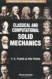
traveled. In choosing a particular path for a tour through the field, one is influenced by the curricular, the trends in literature, and the interest in engineering and science. Here, a particular way has been chosen to view some of the most beautiful vistas in classical and computational mechanics. In making this choice, we have aimed at straightforwardness and interest, and practical usefulness in the long run. Holding the book to a reasonable length did not permit inclusion of many numerical examples, which have to be supplemented through problems and references. Fortunately, there are many excellent references to meet this demand. We have presented an extensive bibliography in this book, but we suggest that the reader consults the review journal Applied Mechanics Reviews (AMR) published by the American Society of Mechanical Engineers International since 1947, for the current information. The reader is referred to the periodic in-depth reviews of the literature in specific issues of AMR. We are indebted to many authors and colleagues as acknowledged in the preface of the Foundations of Solid Mechanics. In the preparation of the present edition, we are especially indebted to Professors Satya Atluri and Theodore Pian. We would like to record our gratitude to many colleagues who wrote us to discuss various points and sent us errata in the Foundations of Solid Mechanics, especially to Drs. Pao-Show D. Cheng, Shun Cheng, Ellis H. Dill, Clive L. Dym, 3. B. Haddow, Manohar P. Kamat, Hans Krumhaar, T. D. Leko, Howard A, Magrath, Sumio Murakami, Theodore Pian, R. S. Rivlin, William P. Rodden, Bertil Storakers, Howard J. White, Jr. and John C. Yao. We would also like to thank professors Y. Ohashi, S. Murakami and N. Kamiya for translating the Foundations book into Japanese, Professors Oyuang Zhang, Ma Wen-Hua and Wang Kai-Fu for translating the Foundations book into Chinese. On the cover of this book, portraits of some pioneers of mechanics are presented. They are arranged, from left to right and top to bottom, according to their birthdays. They are: Galileo Galilei, 1564-1642, Isaac Newton, 1642-1727, Daniel Bernoulli, 1700-1782, Leonhard Euler, 1707-1783, Joseph Louis Lagrange, 1736-1813, Claude Louis Marie Henri Navier, 1785-1836, Augustin Louis Cauchy, 1789-1857, Lord Kelvin, William Thompson, 1824-1907, Gustave Robert Kirchhoff, 1824-1889, Lord Rayleigh, John William Strutt, 1842-1919, Ludwig Edward Boltsmann, 18441906, August Edward Hugh Love, 1863-1940, Stephen P. Timoshenko, 1878-1972. These portraits were supplied by Dr Stephen Juhasz, who was the editor of the Applied Mechanics Reviews for 30 years, from 19531983. In 1973, Dr Juhasz published an article entitled “Famous Mechanics
X
PREFACE
Scientists” in A p p . Mech. Rev. Vol. 26, No. 2. These portraits are from that article, in which acknowledgement to original sources is recorded. We thank you, Dr Juhasz. We would like to take this opportunity to mention a few of editorial notes: (1) The bibliography is given at the end of the book. (2) Equations in each Section are numbered sequentially. When referring to equations in other Sections, we use the format (Sec. no: Eq. no), e.g. (5.6:4). (3) Formulas are concise way of saying lots of things. The most important formulas are marked with a triangular star, A. They are worthy of being committed to memory.
Y. C. F’ung P. Tong
CONTENTS 1
1 INTRODUCTION 1.1. 1.2. 1.3. 1.4. 1.5. 1.6. 1.7. 1.8.
Hooke’s Law Linear Solids with Memory Sinusoidal Oscillations in Viscoelastic Material: Models of Viscoelasticity Plasticity Vibrations Prototype of Wave Dynamics Biomechanics Historical Remarks
Notation and Summation Convention Coordinate Transformation Euclidean Metric Tensor Scalars, Contravariant Vectors, Covariant Vectors Tensor Fields of Higher Rank Some Important Special Tensors The Significance of Tensor Characteristics Rectangular Cartesian Tensors Contraction Quotient Rule Partial Derivatives in Cartesian Coordinates Covariant Differentiation of Vector Fields Tensor Equations Geometric Interpretation of Tensor Components Geometric Interpretation of Covariant Derivatives Physical Components of a Vector
30 33 34 38 39 40 42 43 44 45 46 48 49
52 58 60 66
3 STRESS TENSOR 3.1.
12 14 15 18 22 25
30
2 TENSOR ANALYSIS
2.1. 2.2. 2.3. 2.4. 2.5. 2.6. 2.7. 2.8. 2.9. 2.10. 2.11. 2.12. 2.13. 2.14. 2.15. 2.16.
2 9
66
Stresses xi
xii
CONTENTS
Laws of Motion Cauchy’s Formula Equations of Equilibrium Transformation of Coordinates Plane State of Stress Principal Stresses Shearing Stresses Mohr’s Circles Stress Deviations Octahedral Shearing Stress Stress Tensor in General Coordinates Physical Components of a Stress Tensor in General Coordinates 3.14. Equations of Equilibrium in Curvilinear Coordinates
3.2. 3.3. 3.4. 3.5. 3.6. 3.7. 3.8. 3.9. 3.10. 3.11. 3.12. 3.13.
4 ANALYSIS OF STRAIN Deformation Strain Tensors in Rectangular Cartesian Coordinates Geometric Interpretation of Infinitesimal Strain Components 4.4. Rotation 4.5. Finite Strain Components 4.6. Compatibility of Strain Components 4.7. Multiply Connected Regions 4.8. Multivalued Displacements 4.9. Properties of the Strain Tensor 4.10. Physical Components 4.11. Example - Spherical Coordinates 4.12. Example - Cylindrical Polar Coordinates
4.1. 4.2. 4.3.
5 CONSERVATION LAWS 5.1. 5.2. 5.3. 5.4. 5.5.
Gauss’ Theorem Material and Spatial Descriptions of Changing Configurations Material Derivative of Volume Integral The Equation of Continuity Equations of Motion
69 71 73 78 79 82 85 86 87 88 90 94 95 97
97 100 103 104 106 108 113 117 118 121 123 125
127 127 128 131 133 134
CONTENTS
5.6. 5.7.
Moment of Momentum Other Field Equations
6 ELASTIC AND PLASTIC BEHAVIOR OF MATERIALS 6.1. 6.2. 6.3. 6.4. 6.5. 6.6. 6.7. 6.8. 6.9. 6.10. 6.11. 6.12. 6.13. 6.14. 6.15. 6.16.
Generalized Hooke’s Law Stress-Strain Relationship for Isotropic Elastic Materials Ideal Plastic Solids Some Experimental Information A Basic Assumption of the Mathematical Theory of Plasticity Loading and Unloading Criteria Isotropic Stress Theories of Yield Function Further Examples of Yield Functions Work Hardening - Drucker’s Hypothesis and Definition Ideal Plasticity Flow Rule for Work-Hardening Materials Subsequent Loading Surfaces - Isotropic and Kinematic Hardening Rules Mroz’s, Dafalias and Popov’s, and Valanis’ Plasticity Theories Strain Space Formulations Finite Deformation Plastic Deformation of Crystals
7 LINEARIZED THEORY OF ELASTICITY
7.1. 7.2. 7.3. 7.4. 7.5.
Basic Equations of Elasticity for Homogeneous Isotropic Bodies Equilibrium of an Elastic Body Under Zero Body Force Boundary Value Problems Equilibrium and Uniqueness of Solutions Saint Venant’s Theory of Torsion
xiii
135 136
138
138 140 143 146 150 156 157 159 166 167 171 177 189 195 199 200
203
203 206 207 210 213
xiv
7.6. 7.7. 7.8. 7.9. 7.10.
CONTENTS
Soap Film Analogy Bending of Beams Plane EIastic Waves Rayleigh Surface Wave Love Wave
8 SOLUTIONS OF PROBLEMS IN LINEARIZED THEORY OF ELASTICITY BY POTENTIALS
8.1. 8.2. 8.3. 8.4. 8.5. 8.6. 8.7. 8.8. 8.9. 8.10. 8.11. 8.12. 8.13. 8.14. 8.15.
Scalar and Vector Potentials for Displacement Vector Fields Equations of Motion in Terms of Displacement Potentials Strain Potential Galerkin Vector Equivalent Galerkin Vectors Example - Vertical Load on the Horizontal Surface of a Semi-Infinite Solid Love’s Strain Function Kelvin’s Problem - A SingIe Force Acting in the Interior of an Infinite Solid Perturbation of Elasticity Solutions by a Change of Poisson’s Ratio Boussinesq’s Problem On Biharmonic Functions Neuber-Papkovich Representation Other Methods of Solution of Elastostatic Problems Reflection and Refraction of PIane P and S Waves Lamb’s Problem - Line Load Suddenly Applied on Elastic Half-Space
9 TWO-DIMENSIONAL PROBLEMS IN LINEARIZED THEORY OF ELASTICITY
9.1. 9.2. 9.3. 9.4.
Plane State of Stress or Strain Airy Stress Functions for Two-Dimensional Problems Airy Stress Function in Polar Coordinates General Case
222 224 229 231 235
238
238 241 243 246 249 250 252 254 259 262 263 268 270 270 273
280
280 282 288 295
CONTENTS
9.5.
9.6.
Representation of Two-Dimensional Biharmonic Functions by Analytic Functions of a Complex Variable Kolosoff-Muskhelishvili Method
XV
299 301
10 VARIATIONAL CALCULUS, ENERGY THEOREMS,
SAINT-VENANT'S PRINCIPLE 10.1. 10.2. 10.3. 10.4. 10.5. 10.6. 10.7. 10.8. 10.9. 10.10. 10.11. 10.12. 10.13. 10.14. 10.15.
Minimization of F'unctionals hnctional Involving Higher Derivatives of the Dependent Variable Several Unknown Functions Several Independent Variables Subsidiary Conditions - Lagrangian Multipliers Natural Boundary Conditions Theorem of Minimum Potential Energy Under Small Variations of Displacements Example of Application: Static Loading on a Beam - Natural and Rigid End Conditions The Complementary Energy Theorem Under Small Variations of Stresses Variational Functionals Fkequently Used in Computational Mechanics Saint-Venant's Principle Saint-Venant 's Principle-Boussinesq-Von Mises-Sternberg Formulation Practical Applications of Saint-Venant 's Principle Extremum Principles for Plasticity Limit Analysis
11 HAMILTON'S PRINCIPLE, WAVE PROPAGATION, APPLICATIONS OF GENERALIZED COORDINATES 11.1. 11.2. 11.3.
Hamilton's Principle Example of Application - Equation of Vibration of a Beam Group Velocity
313 313 319 320 323 325 328 330 335 339 346 355 359 362 365 369
379 379 383 393
xvi
CONTENTS
11.4. 11.5. 11.6. 11.7. 11.8.
Hopkinson’s Experiment Generalized Coordinates Approximate Representation of Functions Approximate Solution of Differential Equations Direct Methods of Variational Calculus
12 ELASTICITY AND THERMODYNAMICS 12.1. 12.2. 12.3. 12.4. 12.5. 12.6. 12.7. 12.8. 12.9.
The Laws of Thermodynamics The Energy Equation The Strain Energy Function The Conditions of Thermodynamic Equilibrium The Positive Definiteness of the Strain Energy Function Thermodynamic Restrictions on the Stress-Strain Law of an Isotropic Elastic Material Generalized Hooke’s Law, Including the Etfect of Thermal Expansion Thermodynamic hnctions for Isotropic Hookean Materials Equations Connecting Thermal and Mechanical Properties of a Solid
396 398 399 402 402
407
407 412 414 416 418 419 421
423 425
13 IRREVERSIBLE THERMODYNAMICS AND
VISCOELASTICITY
428
13.1. 13.2. 13.3. 13.4. 13.5.
428 431 432 436
13.6. 13.7. 13.8. 13.9.
Basic Assumptions One-Dimensional Heat Conduction Phenomenological Relations-Onsager Principle Basic Equations of Thermomechanics Equations of Evolution for a Linear Hereditary MateriaI Relaxation Modes Normal Coordinates Hidden Variables and the Force-Displacement Relationship Anisotropic Linear Viscoelastic Materials
440 444 447 450 454
CONTENTS
14 THERMOELASTICITY 14.1. 14.2. 14.3. 14.4. 14.5. 14.6. 14.7. 14.8. 14.9. 14.10. 14.11. 14.12. 14.13.
Basic Equations Thermal Effects Due to a Change of Strain; Kelvin’s Formula Ratio of Adiabatic to Isothermal Elastic Moduli Uncoupled, Quasi-Static Thermoelastic Theory Temperature Distribution Thermal Stresses Particular Integral: Goodier’s Method Plane Strain An Example - Stresses in a Turbine Disk Variational Principle for Uncoupled Thermoelasticity Variational Principle for Heat Conduction Coupled Thermoelasticity Lagrangian Equations for Heat Conduction and Thermoelasticity
15 VISCOELASTICITY 15.1. 15.2. 15.3. 15.4. 15.5. 15.6.
Viscoelastic Material Stress-Strain Relations in Differential Equation Form Boundary-Value Problems and Integral Transformations Waves in an Infinite Medium Quasi-Static Problems Reciprocity blations
16 LARGE DEFORMATION Coordinate Systems and Tensor Notation Deformation Gradient Strains Right and Left Stretch Strain and Rotation Tensors Strain Rates Material Derivatives of Line, Area, and Volume Elements 16.7. Stresses
16.1. 16.2. 16.3. 16.4. 16.5. 16.6.
xvii
456
456 459 459 461 462 464 466 467 470 473 474 478 48 1 487
487 491 497 500 503
507 514
514 521 525 526 528 529 532
xviii
CONTENTS
16.8. 16.9. 16.10. 16.11. 16.12. 16.13.
Example: Combined Tension and Torsion Loads Objectivity Equations of Motion Constitutive Equations of Thermoelastic Bodies More Examples Variational Principles for Finite Elasticity: Compressible Materials 16.14. Variational Principles for Finite Elasticity: Nearly Incompressible or Incompressible Materials 16.15. Small Deflection of Thin Plates 16.16. Large Deflection of PIates
17 INCREMENTAL APPROACH TO SOLVING SOME NONLINEAR PROBLEMS 17.1. 17.2. 17.3. 17.4. 17.5. 17.6. 17.7. 17.8.
Updated Lagrangian Description Linearized Rates of Deformation Linearized Rates of Stress Measures Incremental Equations of Motion Constitutive Laws 0 Incremental Variational Principles in Terms of T Incremental Variational Principles in Terms of *: Incompressible and Nearly Incompressible Materials 17.9. Updated Solution 17.10. Incremental Loads 17.11. Infinitesimal Strain Theory
18 FINITE ELEMENT METHODS 18.1. 18.2.
18.3. 18.4. 18.5.
Basic Approach One Dimensional Problems Governed by a Second Order Differential Equation Shape hnctions and Element Matrices for Higher Order Ordinary Differential Equations Assembling and Constraining Global Matrices Equation Solving
539 543 548 550 557 562 568 573 581
587 587 590 593 597 598 604 610 612 617 620 622
624 626 629 638 643 651
CONTENTS
xix
18.6. Two Dimensional Problems by One-Dimensional Elements 18.7. General Finite Element Formulation 18.8. Convergence 18.9. Two-Dimensional Shape Functions 18.10. Element Matrices for a Second-Order Elliptical Equation 18.11. Coordinate Transformation 18.12. Triangular Elements with Curved Sides 18.13. Quadrilateral Elements 18.14. Plane Elasticity 18.15. Three-Dimensional Shape Functions 18.16. Three Dimensional Elasticity 18.17. Dynamic Problems of Elastic Solids 18.18. Numerical Integration 18.19. Patch Tests 18.20. Locking-F'ree Elements 18.21. Spurious Modes in Reduced Integration 18.22. Perspective
672 676 679 682 690 702 708 714 726 731 735 750 754
19 MIXED AND HYBRID FORMULATIONS
756
19.1. 19.2. 19.3. 19.4. 19.5. 19.6.
Mixed Formulations Hybrid Formulations Hybrid Singular Elements (Super-Elements) Elements for Heterogeneous Materials Elements for Infinite Domain Incompressible or Nearly Incompressible Elasticity
655 657 664 665
756 760 767 782 782 788
20 FINITE ELEMENT METHODS FOR PLATES AND SHELLS
795
Linearized Bending Theory of Thin Plates Reissner-Mindlin Plates Mixed Functionals for Reissner Plate Theory Hybrid Formulations for Plates Shell as an Assembly of Plate Elements General Shell Elements Locking and Stabilization in Shell Applications
795 805 813 819 822 832 843
20.1. 20.2. 20.3. 20.4. 20.5. 20.6. 20.7.
XX
CONTENTS
21 FINITE ELEMENT MODELING OF NONLINEAR
ELASTICITY, VISCOELASTICITY, PLASTICITY, VISCOPLASTICITY AND CREEP 21.1. 21.2. 21.3. 21.4. 21.5. 21.6. 21.7. 21.8.
Updated Lagrangian Solution for Large Deformation Incremental Solution Dynamic Solution Newton-Raphson Iteration Method Viscoelasticity Plasticity Viscoplasticity Creep
849 852 854 855 857 859 869 870
BIBLIOGRAPHY
873
AUTHOR INDEX
909
SUBJECT INDEX
919
1 INTRODUCTION Mechanics is the science of force and motion of matter. Solid mechanics is the science of force and motion of matter in the solid state. Physicists are of course interested in mechanics. The greatest advances in physics in the twentieth century are identified with mechanics: the theory of relativity, quantum mechanics, and statistical mechanics. Chemists are interested in the mechanics of chemical reaction, the formation of molecular aggregates, the formation of crystals, or the creation of new materials with desirable properties, or polymerization of larger molecules, etc. Biologists are interested in biomechanics that relates structure to function at all hierarchical levels: from biomolecules to cells, tissues, organs, and individuals. Although a living cell is not a homogeneous continuum, it is a protein machine, a protein factory, with internal machinery that moves and functions in an orderly way according to the laws of mechanics. Therefore, all scientists are interested in mechanics and mechanics is developed by scientists continuously. Engineers, especially aeronautical, mechanical, civil, chemical, materials, biomedical, biotechnological, space, and structural engineers, are real developers and users of fluid and solid mechanics because of their professional needs. They design. They invent. They are concerned about the safety and economy of their products. They want to know the function of their products its precisely as possible. They want results fast. They experiment. They theorize. They test, compute, and validate. To them mechanics is a toy, a bread and butter, a feast or delicacy. Engineering is quite different from science. Scientists try to understand nature. Engineers try to make things that do not exist in nature. Engineers stress invention. To embody an invention the engineer must put his idea in concrete terms, and design something that people can use. That something can be a device, a gadget, a material, a method, a computing program, an innovative experiment, a new solution to a problem, or an improvement on what is existing. Since a design has to be concrete, it must have its geometry, dimensions, and characteristic numbers. Almost all engineers working on new designs find that they do not have all the needed information. Most 1
2
INTRODUCTION
Chap. 1
often, they are limited by insufficient scientific knowledge. Thus they study mathematics, physics, chemistry, biology and mechanics. Often they have to add to the sciences relevant to their profession. Thus engineering sciences are born. This book is written by engineering scientists, for engineering scientists, and this determines its style. The qualities we want are: 0 0 0 0 0
Easy to read, Precise, concise, and practical, First priority on the formulation of problems, Presenting the classical results as gold standard, and Numerical approach as everyday tool to obtain solutions.
If the book is a banquet, we offer some hors d’oeuvres in this introductory chapter. 1.1. HOOKE’S LAW
Historically, the notion of elasticity was first announced in 1676 by Robert Hooke (1635-1703) in the form of an anagram, ceiiinosssttuw. He explained it in 1678 as U t tensio sic v i s ,
or “the power of any springy body is in the same proportion with the extension.” t As stated in the original form, Hooke’s law is not very clear. Our first task is to give it a precise expression. Historically, this was done in two different ways. The first way is to make use of the common notion of “springs,” and consider the load-deflection relationship. The second way is to state it as a tensor equation connecting the stress and strain. Although the second way is the proper way to start a general theory, the first, simpler and more restrictive, is not without interest. In this section, we develop the first alternative as a prototype of the theory of elasticity. Let us consider the static equilibrium state of a solid body under the action of external forces (Fig. 1.1:l). Let the body be supported in some manner so that at least three points are fixed in a space which is described with respect to a rectangular Cartesian frame of reference. We shall make three basic hypothesis regarding the properties of the body under considerat ion.
(Hl) The body is continuous and remains continuous under the action of external forces. t Edme Mariotte enunciated the same law independently in 1680.
Sec. 1.1
HOOKE’SLAW
3
Under this hypothesis the atomistic structure of the body is ignored and the body is idealized into a geometrical copy in Euclidean space whose points are identified with the material particles of the body. Continuity is defined in mathematical sense as an isomorphism of the real number system. Neighboring points remain as neighbors under any loading condition. No cracks or holes may open up in the interior of the body under the action of external load. A material satisfying this hypothesis is said to be a continuum. The Fig. 1.1:l. Static equilibrium of a study of the deformation or motion of body under external forces. a continuum under the action of forces is called the continuum mechanics. To introduce the second hypothesis, let us consider the action of a set of forces on the body. Let every force be fixed in direction and in point of application, and let the magnitude of all the forces be increased or decreased together: always bearing the same ratio to each other. Let the forces be denoted by PI,Pa,. . . , P n and their magnitude by PI,P2, . . . ,Pn. Then the ratios PI : P2 : . .. : P,, remain fixed. When such a set of forces is applied on the body, the body deforms. Let the displacement at an arbitrary point in an arbitrary direction be measured with respect to a rectangular Cartesian frame of reference fixed with the supports. Let this displacement be denoted by u. Then our second hypothesis is
(H2)Hooke’s law;
where al, a2,. . . ,a, are constants independent of the magnitude of PI, Pz,. .. ,P,. The constants a l l a2,. . . ,a, depend, of course, on the location of the point at which the displacement component is measured and on the directions and points of application of the individual forces of the loading. Hooke’s law in the form (H2)is one that can be subjected readily to direct experimental examination. To complete the formulation of the theory of elasticity, we need a third hypothesis:
4
Chap. 1
INTRODUCTION
(H3) There exists a unique unstressed state of the body, to which the body returns whenever all the external forces are removed.
A body satisfying these three hypothesis is called a linear elastic solid. A number of deductions can be drawn from these assumptions. We shall list a few important ones. (A) Principle of superposition By a combination of (H2) and (H3), we can show that Eq. (1) is valid not only for systems of loads for which the ratios PI : P2 : . . . : P, remain fixed as originally assumed, but also for an arbitrary set of loads P I ,P2, . . . ,P,. In other words, Eq. (1) holds regardless of the order in which the loads are applied.
Proof. If a proof of the statement above can be established for an arbitrary pair of loads, then the general theorem can be proved by mathematical induction. Let P1 and P2 (with magnitudes PI and P2) be a pair of arbitrary loads acting at points 1 and 2, respectively. Let the deflection in a specific direction be measured at a point 3 (see Fig. 1.1:l). According to (H2), if P1 is applied alone, then a t the point 3 a deflection u3 = ~ 3 P1 1 is produced. If Pz is applied alone, a deflection u3 = c32P2 is produced. If P1 and Pa are applied together, with the ratio PI : Pz fixed, then according to (H2) the deflection can be written as
(4
u3
= C k 1 Pl
+
CL2
P2 .
The question arises whether cil = ~ 3 1 cb2 , = ~ 3 2 . The answer is affirmative, as can be shown as follows. After P1 and P2 are applied, we take away P I . This produces a change in deflection, -c&P1, and the total deflection becomes (b)
u3 = C k 1 Pl
+ Ck2P2
-
c;1 Pl .
Now only P2 acts on the body. Hence, upon unloading Pz we shall have
Now all the loads are removed, and Rearranging terms, we have
u3
must vanish according to (H3).
Since the only possible difference of cbl and c& must be caused by the action of P z , the difference cil - cgl can only be a function of P2 (and not
Sec. 1.1
HOOKE’SLAW
of PI). Similarly, ~ 3 -2 cL2 can only be a function of as
6
4. If we write Eq. (d)
then the left-hand side is a function of P2 alone, and the right-hand side is a function of PI alone. Since PI and Pz are arbitrary numbers, the only possibility for Eq. (e) to be valid is for both sides to be a constant k which is independent of both PI and P2. Hence,
But a substitution of (f) into (a) yields
The last term is nonlinear in P I , P2, and Eq. (g) will contradict (H2) unless k vanishes. Hence, k = 0 and ci2 = ~ 3 2 .An analogous procedure shows C i l = cp1 = c31. Thus the principle of superposition is established for one and two forces. An entirely similar procedure will show that if it is valid for m forces, it is also valid for m 1 forces. Thus, the general theorem follows by mathematical induction. Q.E.D. The constants ~ 3 1 ~, 3 2 etc., , are seen to be of significance in defining the elastic property of the solid body. They are called influence coeficients or, more specifically, flexibility influence coefficients.
+
(B) Corresponding forces and displacements and the unique meaning of the total work done by the forces. Let us now consider a set of external forces P I ,. . . ,P, acting on the body and define the set of displacements at the points of application and in the direction of the loads as the displacements “corresponding” to the forces at these points. The reactions at the points of support are considered as external forces exerted on the body and included in the set of forces. Under the loads P I , .. . , P,, the corresponding displacements may be written as u1 = C11Pl
(2)
212
= C21Pl
+ c12P2 + .. + + c22P2 + + %Pn, *
ClnPn,
‘ * .
...... ............................
21n=cn1P1 + c n 2 P 2 + * * * + c n n P n .
6
Chap, 1
INTRODUCTION
If we multiply the first equation by P I , the second by P2, etc., and add, we obtain (3)
9.1
+ P2u2 + . . . + Pnu, = CllP? + C12PlP2 + . . + ClnPlP, + C21PlP2 + c22Pz”+ . . . + c,,P,2. *
The quantity above is independent of the order in which the loads are applied. It is the total work done by the set of forces.
( C ) Maxwell’s reciprocal relation The influence coeficients for correspondingforces and displacements are symmetric. c%J. . - c3,2, * (4) In other words, the displacement at a point i due to a unit load at another point j is equal to the displacement at j due to a unit load at a, provided that the displacements and forces ‘%orrespond,”i.e., that they are measured in the same direction at each point. The proof is simple. Consider two forces P1 and P2 (Fig. 1.1:l).When the forces are applied in the order P I , P2, the work done by the forces is easily seen to be
W
=
1 -(C11P,” c22P3 2
+
+ Cl2PlP2.
When the order of application of the forces is interchanged, the work done is 1 W’ = -(C22r)22 CllP,”) C21PlPZ. 2
+
But according to (B) above, W and the theorem is proved.
= M”
+
for arbitrary P I ,P2. Hence, c12 = c21,
(D) Betti-Rayleigh reciprocal theorem Let a set of loads P I ,P2, . . . , P , produce a set of corresponding displacements u1, u2,. . . ,u,. Let a second set of loads P i , P h , . . . ,PL, acting in the same directions and having the same points of application as those of the first, produce the corresponding displacements ui,ui,. . . , uk. Then (5)
Plu:
+ P 2 U k + . . . + P,.:,
= P[u, + * . .
+ P{u,,
In other words, in a linear elastic solid, the work done by a set of forces acting through the corresponding displacements produced by a second set of
Sec. 1.1
HOOKE'SLAW
7
forces is equal to the work done by the second set of forces acting through the corresponding displacements produced by the first set of forces. A straightforward proof is furnished by writing out the u( and u: in terms of Pi and Pi, (i = 1,2,. . . , n ) , with appropriate influence coefficients, comparing the results on both sides of the equation, and utilizing the symmetry of the influence coefficients. In the form of Eq. ( 5 ) , the reciprocal theorem can be generalized to include moments and rotations as the corresponding generalized forces and generalized displacements. An illustration is given in Fig. 1.1:2. These theorems are very useful in practical applications.
For the same beom, cPf= ct2. ( a ) Forces and corresponding displacements.
(b) Generolized force (moment) and the corresponding generolized displocement (moment -rotation of angle).
Fig. 1.1:2. Illustration of the reciprocal theorem.
(E)Strain energy Further insight can be gained from the first law of thermodynamics. When a body is thermally isolated and thermal expansions are neglected the first law states that the work done on the body by the external forces in a certain time interval is equal to the increase in the kinetic energy and internal energy in the same interval. If the process is so slow that the kinetic energy can be ignored, the work done is seen to be equal to the change in internal energy. If the internal energy is reckoned as zero in the unstressed state, the stored internal energy shall be called strain energy. Writing U for the
8
Chap. 1
INTRODUCTION
strain energy, we have, from (3) and (4),
If we differentiate Eq. (6) with respect to Pi,we obtain i = 1 , 2 , . * . ,72. But, the right-hand side is precisely ui;hence, we obtain
(F) Castigliano’s theorem (7)
dU dPa
-=ua,
i = l , ..., n.
In other words, if a set of loads P I , . . . , P, is applied on a perfectly elastic body as described above and the strain energy is expressed as a function of the set P I , .. , , P,, then the partial derivative of the strain energy, with respect to a particular load, gives the corresponding displacement at the point of application of that particular load in the direction of that load.
(E) The principle of virtual work On the other hand, for a body in equilibrium under a set of external forces, the principle of virtual work can be applied to show that, i f the strain energy is expressed as a function of the corresponding displacements, then
dU
- =Pa, dUi
i
=
1,..., n
The proof consists in allowing a virtual displacement 6u to take place in the body in such a manner that Su is continuous everywhere but vanishes at all points of loading except under P , . Due to 6u, the strain energy changes by an amount 6 U , while the virtual work done by the external forces is the product of Pi times the virtual displacement, i.e., P i h i . According to the principle of virtual work, these two expressions are equal, SU = Pidui.On rewriting it in the differential form, the theorem is established. The important result (8) is established on the principle of virtual work as applied to a state of equilibrium under the additional assumption that a strain energy function that is a function of displacement exists. It is a p plicable also to elastic bodies that follow the nonlinear load-displacement relationship.
Sec. 1.2
LINEAR SOLIDS WITH MEMORY: MODELS OF
...
9
1.2. LINEAR SOLIDS WITH MEMORY: MODELS OF VISCOELASTICITY
Most structural metals are nearly linear elastic under small strain, as measurements of load-displacement relationship reveal. The existence of normal modes of free vibrations which are simple harmonic in time, is often quoted as an indication (although not as a proof) of the linear elastic character of the material. However, when one realizes that the vibration of metal instruments does not last forever, even in a vacuum, it becomes clear that metals deviate somewhat from Hooke’s law. Thus, other constitutive laws must be considered. The need for such an extension becomes particularly evident when organic polymers are considered. In this section we shall consider a simple class of materials which retains linearity between load and deflection, but the linear relationship depends on a third parameter, time. For this class of material, the present state of deformation cannot be determined completely unless the entire history of loading is known. A linear elastic solid may be said to have a simple memory: it remembers only one configuration; namely, the unstrained natural state of the body. Many materials do not behave this way: they remember the past. Among such materials with memory there is one class that is relatively simple in behavior. This is the class of materials named above, for which the cause and effect are linearly related.
Fig. 1.2:l. Models of linear viscoelasticity: (a) Maxwell, (b) Voigt, (c) Kelvin.
Let us consider some simple examples. In Fig. 1.2:l are shown three mechanical models of material behavior, namely, the Maxwell model, the Voigt model, and the Kelvin model, all of which are composed of combinations of linear springs with spring constant p and dashpots (pistons moving in a viscous fluid) with coefficient of viscosity q. A linear spring is s u p posed to produce instantaneously a deformation proportional to the load. A dashpot is supposed to produce a velocity proportional to the load at any instant. The load-deflection relationship for these models are
Chap. 1
10
INTRODUCTION
(1)
Maxwell model:
(2)
Voigt model:
(3)
Kelvin model:
F
u=-+-
F
P r l
+ qU, F +T ~ = F ER(U+ T , I ~ ) , F
= PU
u(0)= 0 ,
T,F(O) = ERT,u(O),
where T ~T~, are two constants. When these equations are t o be integrated, the initial conditions at t = 0 must be prescribed as indicated above. The creep functions c ( t ) , which are the displacement u ( t ) in response to a unit-step force F ( t ) = l ( t ) defined in Eq. (7) below, are the solution of Eqs. (1)-(3). They are: (4) Maxwell solid:
c(t) =
(1+ ' t ) P r l
l(t),
(5)Voigt solid:
(6) Kelvin solid:
where the unit-step function l ( t ) is defined as
(7)
l(t)
=
i: 1
when t > O ,
-
when t = 0 ,
0
when t < O .
A body which obeys a load-deflection relation like that given by Maxwell's model is said to be a Maxwell solid. Similarly, Voigt and Kelvin solids are defined. These models are called models of wiscoelasticity. Interchanging the roles of F and u , we obtain the relaxation function as a response F ( t ) = k ( t ) corresponding to an elongation u(t)= l ( t ) ,Eq. (7). ( 8 ) Maxwell solid:
k ( t ) = pe-(p'q)'l(t), (9) Voigt solid:
k ( t ) = 176(t) + P q t ) 1
Sec. 1.2
LINEAR SOLIDS WITH MEMORY: MODELS OF
...
11
(10) Kelvin solid:
Here we have used the symbol s ( t ) to indicate the unit-impulse function, or Dimc-delta function, which is defined as a function with a singularity at the origin:
qt)=0
(‘ f(t)b(t)dt= f(0) ,
for t
< 0, and t > 0 , E > O ,
J--E
where f ( t ) is an arbitrary function continuous at t = 0. These functions, c(t)and k(t),are illustrated in Figs. 1.2:2 and 1.2:3, respectively, for which we add the following comments.
Fig. 1.2:2. Creep function of (a) Maxwell, (b) Voigt, (c) Kelvin solid. A negative phase is superposed at the time of unloading.
For the Maxwell solid, a sudden application of a load induces an immediate deflection by the elastic spring, which is followed by “creep” of the dashpot. On the other hand, a sudden deformation produces an immediate reaction by the spring, which is followed by stress relaxation according to an exponential law Eq. (8). The factor ~ / p with , dimengions of time, may be called a relaxation time: it characterizes the rate of decay of the force. For the Voigt solid, a sudden application of force will produce no immediate deflection because the dashpot, arranged in parallel with the spring, will not move instantaneously. Instead, as shown by Eq. (5) and Fig. 1.2:2(b), a deformation will be gradually built up, while the spring takes a greater and greater share of the load. The dashpot displacement relaxes exponentially. Here the ratio q / p is again a relaxation time: it characterizes the rate of decay of the deflection.
12
Chap. 1
INTRODUCTION
al
e
l.2 E
L
0
.c 0)
Q ‘0
Time
I Time
Fig. 1.2:3. Relaxation function, of (a) Maxwell, (b) Voigt, (c) Kelvin solid.
For the Kelvin solid, a similar interpretation is applicable. The constant rEis the time of relaxation of load under the condition of constant deflection [see Eq. (lo)], whereas the constant ro is the time of relaxation of deflection under the condition of constant load [see Eq. (4)]. As t -+ 00, the dashpot is completely relaxed, and the load-deflection relation becomes that of the springs, as is characterized by the constant ER in Eqs. (4) and (10). Therefore, ER is called the relaxed elastic modulus. Load-deflection relations such as (1)-(3) were proposed t o extend the classical theory of elasticity to include anelastic phenomena. Lord Kelvin (Sir William Thomson, 1824-1907), on measuring the variation of the rate of dissipation of energy with frequency of oscillation in various materials, showed the inadequacy of the Maxwell and Voigt equations. A more successful generalization using mechanical models was first made by John H. Poynting (1852-1914) and Joseph John Thomson (“J.J.,”1856-1940) in their book Properties of Matter (London: C . Griffin and Co., 1902). 1.3. SINUSOIDAL OSCILLATIONS IN A VISCOELASTIC
MATERIAL
It is interesting to examine the relationship between the load and the deflection in a body when it is forced t o perform simple harmonic oscillations. A simple harmonic oscillation can be described by the real or imaginary part of a complex variable. Thus, if Fo is a complex variable FO= Aeib = A(cos 4 + i sin d), then a simple harmonic oscillatory force can be written as (1)
F ( t ) = FoeiWt = A(cos4 + isin4)(coswt + isinwt) = A cos(wt
+ 4) + i A sin(wt + 4) .
Sec. 1.3
SINUSOIDAL OSCILLATIONS IN A VISCOELASTIC
...
13
Similarly, if uo = Bei$, then a simple harmonic oscillatory displacement u(t)= uOeiWt is either the real part or the imaginary part of (2)
u ( t )= uOeiWt = B cos(wt + $1
+ i~
sin(wt
+ $) .
On substituting (1) and (2) into Eqs. (1)-(3) of Sec. 1.2, we can obtain the is called the ratio uo/Fo, which is a complex number. The inverse, FO/UO, complex modulus of a viscoelastic material, and is often designated by M :
M
(3)
= FO/UO = lMleis
where [MI is the magnitude and 6 is the phase angle by which the strain lags behind the stress. The tangent of 6 is often used as a measure of the internal friction of a linear viscoelastic material: tan6 =
(4)
imaginary part of M real part of M
*
For the Kelvin model, we have (5)
M = 1 + iwr,
1 + iwr,
ER
1
IMI= ( 1 + w 2 r ~ ) 1 ' 2 E R , 1 f w".,"
When [MI and t an 6 in (5) and ( 6 ) are plotted against the logarithm of w , curves as shown in Fig. 1.3:l are obtained. Experiments with torsional
-
-. c .c ,n
I
I
I
I
Internal friction
I -
0 Y
.- 2
0.01
0.I
10
100
0-
Fig. 1 3 1 . Frequency dependence of internal friction and elastic modulus.
14
Chap. 1
INTRODUCTION
Frequency
Fig. 1.3:2. A typical relaxation spectrum. (After C. M. Zener, Elasticity and Anelasticity of Metals, The University of Chicago Press, 1948.)
oscillations of metal wires a t various temperatures, reduced to room temperature according t o certain thermodynamic formula, yield a typical “relaxation spectrum” as shown in Fig. 1.3.2. Many peaks are seen in the internal-friction-versus-frequency curve. It has been suggested that each peak should be regarded as representing an elementary process as described above, with a particular set of relaxation times T,, rE.Each set of relaxation times T,, T~ can be attributed t o some process in the atomic or microscopic level. A detailed study of such a relaxation spectrum tells a great deal about the structures of metals; and the study of internal friction has provided a very effective key to metal physics. 1.4. PLASTICITY
Take a small steel rod. Bend it. When the deflection is small, the rod will spring back to its original shape when you release the load. This is elasticity. When the deflection is sufficiently large, a permanent deformation will remain when the load is released. That is plasticity. The load-deflection relationship of an ideal plastic material is shown in Fig. 1.4:1(a). For an ideal plastic material, the deflection is zero when the load is smaller than a critical value. Then, when the load reaches a critical value, the deflection continues to increase (the material flows) as long as the same load remains. If, a t a given deflection, the load becomes smaller than the critical value, then the flow stops. There is no way the load can be increased beyond the critical value.
Sec. 1.5
VIBRATIONS
..il. Deflection
Deflection (a) Ideal plasticity
15
(b) Linear elastic
- ideal
plastic material
Fig. 1.4:l.
Structural steel behaves pretty much like an ideal plastic material, except that when the load (measured in terms of the maximum shear stress) is smaller than the critical load (called the yield shear stress), the loaddeflection curve is an inclined straight line (Hooke’s Law). Upon unloading, there is a small rebound. There are some details at the yield point that were ignored in the statement above. Other metals, such as copper, aluminum, lead, stainless steel, etc., behave in a somewhat similar, but more complex manner. Metals at a sufficiently high temperature may behave more like a fluid. Theories that deal with these features of materials are called the theories of plasticity, which are presented in Chapter 6 . 1.5. VIBRATIONS
We know vibrations by experience while driving a car, flying an airplane, playing a musical instrument. The trees sway in the wind. A building shakes in an earthquake. Sometimes we want to know if a structure is safe in vibration. Sometimes we want to design a cushion that isolates an instrument from vibrations. A prototype of this kind of problem is shown in Fig. 1.5:1(a). A body with mass M is attached to an initially vertical massless spring, which has a spring constant k, and a damping constant c, and is “built-in” to a “ground” which moves horizontally with a displacement history s ( t ) . Let x ( t ) denote the horizontal displacement of the mass and a dot over x or s denote a differentiation with respect to time. Then 2 is the acceleration of the body, k ( x - s ) is the spring force acting on the body, and c(k - S) is the viscous damping force acting on the body. Newton’s second law requires that (1)
MX + ~ ( -2S) + k ( -~ S) = 0 .
If we let (2)
y=x-s,
16
Chap. 1
INTRODUCTION
Fig. 1.5:l.
represent the displacement of the body relative to the ground, then Eq. (1) may be written as
(3)
My+cy+ky=-Ms.
The solution of Eq. (3) represents a forced vibration of a damped system. If the forcing function MS(t) were zero, the equation (4)
My + qj + Icy = 0 ,
describes the free vibration of the damped system. If the damping constant c vanishes, then the free vibration of the undamped system is described by the equation (5) My+ky = 0. Equation (5) is satisfied by the solution (6)
y = Acoswt
+ Bsinwt,
in which A and B are arbitrary constants, and
(7)
w=
m,
as can be verified by direct substitution of ( 6 ) into (5). When k and M are real values, w is real. The motion y(t) given by (6) is an oscillation of the
Sec. 1.5
VIBRATIONS
17
body at a circular frequency of w rad/sec. It can exist without external load. Hence w is called the natural frequency of a free vibration. If the damping constant c were zero, and the forcing function i is periodic with the same frequency as the natural one, then the amplitude of the oscillation is unbounded, and we have the phenomenon of resonance. The solution of Eq. (4) must be an exponential function of time, because the derivative of an exponential function is another exponential function. Thus y(t) = Ae"
(8)
implies y ( t ) = AXe"
,
y(t) = A X 2 e x t .
On substituting (8) into Eq. (4),we have
MA2 + C X + k
(9)
= 0.
If we write k/M
(10)
=w 2 ,
&
=c/
(2&7),
then the two roots of Eq. (9) may be written as XI and (11)
X I = -&W
+ i W J S ,
Xz = -&W
-
X2:
iwJ1-E2.
When k and M are real positive numbers, w is real, and the solution of Eq. (9) under the initial conditions
(12)
y(0) = yo ,
y(0) = yo when t = 0 .
is (13)
y ( t ) = yoe--EW t c o s w & 2 t
Now, we can return to the solution of Eq. (3). A particular solution of Eq. (3) can be obtained by Laplace or Fourier transformation or other methods. By direct substitution, it can be verified that a particular solution satisfying the initial conditions y(t) = y ( t ) = 0 at t = 0 is:
The general solution of Eq. (3) is the sum of the functions given in (13) and (14). From this solution we can examine the nature of the forced oscillation
18
INTRODUCTION
Chap. 1
and its dependence on the parameters w ,E , and the frequency spectrum of the forcing function s(t). The simple solution given by Eqs. (13) and (14) has important applications to the problems of isolation of delicate instruments in shipping, response of buildings to earthquake, impact of an airplane on landing, landing a robot on the moon. A frequently asked quention is: what is the maximum absolute value of the displacement y, or the acceleration jj as functions of the peak values of the ground displacement s, ground acceleration 6, the time course of the ground motion, the system characteristis MI c , k, and the initial conditions yo, Ij, ie., (15)
max I y ( t ) l / max Is(t)l = f u n c t i o n of .s(t), M , c, Ic, yo, Ij, max Iy(t)l/ max Is(t)l = f u n c t i o n s of s ( t ) ,MIc , C,yo,yo .
These functions are called shock spectra. Studies of shock spectra are important not only for technological applications, but also for mathematics. Note that although Eq. (3) is linear in y ( t ) , the shock spectra are nonlinear functions of the parameters of the system. Qualitatively, we notice that the most important characteristic time of the system. Qualitatively, we notice that the most important characteristic time of the free oscillation is l/w.The most important characteristic time of the excitation s ( t ) is the length of time it takes to rise from 0 to the peak value, t,. We call t, the rise tame of the signal. Alluring to resonance, we see that a parameter of importance is the ratio of the two charateristic times l / w and t,. Hence the shock spectra are principally functions of wt,. See some references in the bibliography at the end of the book. The picture shown in Fig. 1.5:1(b) may represent, in a very crude way, a concrete floor of a steel frame building during an earthquake. A system shown in Fig. 1.5:1(c) may represent an astronaut in flight. A dumbbell shown in Fig. 1.5:1(d) has been used to model a molecule. It is clear that fairly comprehensive models of dynamic systems can be devised by this approach, see, for example, Fig. 1.5:1(e). When there are too many particles of mass and springs of elasticity, however, simplicity may be lost, and one turns naturally to the continuum approach outlined in the next section. 1.6. PROTOTYPE OF WAVE DYNAMICS
A wire with an infinite number of particles of mass connected together elastically is an obvious candidate for the continuum approach. As an example, consider a wire as shown in Fig. 1.6:l. Let an axis z run along
Sec. 1.6
PROTOTYPE OF WAVE DYNAMICS
19
Fig. 1.6:l.
Fig. 1.6:2.
the length of the wire, with an origin 0 chosen at the lower end. When the wire is loaded, each particle in the wire will be displaced longitudinally from its original position by an amount u. We shall consider only axial loading and assume that the plane cross sections remain plane, so that u is parallel to the x-axis and is a function of z. We shall assume further that u is infinitesimal, so that the strain in the wire is
The change in cross-sectional dimensions of the wire due to the axial load will be ignored. The wire is assumed to be elastic, and is so thin that all stress components other than the axial may be neglected. Then the axial stress is given by Hooke’s law dU
0
= Ee = E - ,
dX in which E is a constant called the Young’s modulus of elasticity. Now consider an element of the wire of a small length dx (see Fig. 1.6:2). The
20
Chap. 1
INTRODUCTION
force acting at the lower end is u A , where A is the cross-sectional area of the wire. The force acting a t the upper end is A ( a da). For a continuous function a(.) the differential da is equal to (da/dx)dx. The acceleration of the element, d2u/dt2,must be caused by the difference in axial forces. Now, the mass of the element is pAdx, with p denoting the density of the material. Hence, equating the mass times acceleration with the axial load Ada, and canceling the nonvanishing factor Adz, we obtain the equation of motion a2u aa p-=(3) at2 ax
+
A substitution of Eq. (2) yields the wave equation (4)
in which the constant c is the wave speed:
(5) The wave speed c is a characteristic constant of the material. The general solution of Eq. (4) is
u = f ( -~Ct)
(6)
+ F ( x + ct) ,
where f and F are two arbitrary functions. This can be verified by substituting Eq. (6) directly into Eq. (4). The function u = f ( x - ct) represents a wave propagating in the positive x direction. The function u = F ( z c t ) represents a wave propagating in the negative x direction. In either case we have
+
with u = &/at denoting the particle velocity. A substitution of (7) and (5) into (2) yields the formula
a
(8)
=
E
f-w
= fpcv,
C
where the - sign applies to a wave propagating in the positive x direction, and the sign applies to a wave in the other direction. This result is remarkable. It says that the stress is equal to the product of the mass density of the material, the velocity of the sound wave, and the longitudinal velocity of the particles of the wire. This result has a very important
+
Sec. 1.6
PROTOTYPE OF WAVE DYNAMICS
21
application to an experiment initiated by John Hopkinson (1872) who hang a steel wire vertically from a ceiling, attached a stopper at the lower end as shown in Fig. 1.6:1, then dropped a massive weight down the wire from a measured height. When the weight struck the stopper, it stretches the wire suddenly. Hopkinson’s intention was to measure the strength of the wire with this method. Using different weights dropped from different heights, he found that the minimum height from which a weight had to be dropped to break the wire was, within certain limits, almost independent of the magnitude of the weight, and the diameter of the wire. Now, when different solid bodies are dropped from a given height, the velocity reached at any given time is independent of the weight. Thus Hopkinson explains his result on the basis of elastic wave propagation. Equation (8) shows that the stress is equal to pcw. The speed of sound of longitudinal waves in the wire, given by Eq. (5) is 16,000 ft/sec for steel. The velocity t~ in the wire, however, is not necessarily the largest at the instant of impact at the lower end. To find w , we have to solve Eq. (4)with the boundary conditions of the Hopkinson experiment (Fig. 1.6:1), which has a clamped upper end, and a movable lower end: (9)
at x
u=o
=L
for all t , and
(16)
when t 5 0 for all x , (10) (11)
dV M-=A dt
0
V = VO
at x = 0 for all t ,
(17)
at x = 0 when t = 0 .
(18)
Here VOis the velocity of the stopper, and A4 is the combined mass of the dropped weight and the stopper. The mathematical problem is reduced to finding the arbitrary function f(x - c t ) and F ( x c t ) so that u ( x ,t ) given by Eq. (6) satisfies Eqs. (9)-(11). Physically, the weight generated an elastic wave u(x,t ) in the wire initiated by a velocity VOat x = 0 when t = 0. The wave went up, reflected at the top, went down, reflected at the lower end by the moving weight, and so on. In John Hopkinson’s test, a 27-foot long wire and weights ranging from 7 to 41 lbs. were used, and the absolute maximum of v and u was reached at the top after a number of reflections. The stress picture was very complicated. Bertram Hopkinson (1905) repeated his father’s experiment with a 1 lb. weight impacting on the lower end of a 30-foot long No. 10 gauge wire weighing 1.3 lbs. Nevertheless, as shown by G. I Taylor (1946), the maximum tensile stress in B. Hopkinson’s experiment did not occur at the
+
22
INTRODUCTION
Chap. 1
first reflection, when the stress was 2pcV0, but at the third reflection, Le., the second reflection at the top of the wire, when the tensile stress reached 2.15 pCV0. If the mass of the wire were negligible, then the wave velocity is very high and the system of Fig. 1.6:l would become a mass and spring system of Sec. 1.5. Thus waves and vibrations are different features of the same dynamic system. Waves deliver extremely important information in a solid body. They are used in geophysics to probe the earth, to study earthquakes and to find oil and gas reserves. In medicine the pulse waves in the artery and the sound waves in the lung are used for diagnosis. In music the piano tuner and violin player listen to the vibration characteristics of their instruments. Some aspects of the general theory are discussed in Chapter 9. 1.7. BIOMECHANICS
Historically, the theory of solid mechanics was first developed along the lines of the linearized theory of elasticity, then it was expanded to the linearized theory of viscoelasticity. Then plasticity came on the scene. The nonlinear theory of large deformation and finite strain was developed. Further expansion was made possible by computational methods. Many significant problems in material science, aerospace structures, metal and plastics industries, geophysics, planetary physics, thermo-nuclear reactors, etc., were solved. Following this trend of expansion, it is natural t o consider biological problems. Many mechanics scientists had contributed to the understanding of physiology, e.g: Galileo Galilei (1564-1642), William Harvey (1578-1658), Ren6 Descartes (1596-1650), Giovanni Alfonso Borelli (1608-1679), Robert Boyle (1627-1691), and Robert Hooke (1635-1703) before Newton (16421727), and Leonhard Euler (1707-1783), Thomas Young (1773-1829), Jean Poiseuille (1797-1869), Herrmann von Helmholtz (1821-1894) after Newton. In fact, the Greek book On the Parts of Animals written by Aristotle (384-322 BC) and the Chinese book Nei Jing (or Internal Classic) attributed to Huangti (Yellow Emperor), but was believed to be written by anonymous authors in the Warring Period (472-221 BC), contain many concepts of biomechanics. At the time when the manuscript of the first edition of this book was prepared, the molecule that is responsible for the genetics of the cells had been identified as DNA, and the double helix structure of DNA had been discovered. The beginning of a new age of understanding biology in t e r m of chemistry, physics and mechanics was recognized by many people.
Sec. 1.7
BIOMECHANICS
23
Biomechanics has the following salient features:
(1) Material Constitution Every living organism has a solid structure that gives it a unique shape and size, and an internal fluid flow that transports materials and keep the organism alive. Hence biosolid mechanics is inseparable from biofluid mechanics. The cells make new materials. Hence the composition, structure, and ultrastructure of biomaterials change dynamically. (2) The Constitutive Equations
Blood is a non-Newtonian fluid. Synovial fluid in the knee joint, and body fluid in the abdominal cavity are also non-Newtonian. The bone obeys Hooke’s law. The blood vessel, the skin and most other soft tissues in the body do not obey Hooke’s law. We must know the constitutive equations of biological tissues, whose determination was a major task of the early biomechanics. When attention is focused on cells, the determination of the constitutive equations of DNA and other molecules becomes a primary task. (3) Growth and Remodeling of Living Tissues Under Stress
Tissue is made of cells and extracellular matrices. The cetl division, growth, hypertrophy, movement, or death are influenced by the cell geometry and the stress and strain in the cell, as well as by the chemical and physical environment. The tissue is, therefore, a changing, living entity. The determination of the growth law is a major task in biology. (4) The Existence of Residual Stress
Organs such as the blood vessel, heart, esophagus and intestine have large residual strain and stress at the no-load condition. The residual strain changes in life because any birth or death of a cell in a continuum and the building and resorption of extracellular matrix by the cells create residual strains in the continuum. The changes of residual stress and strain cause changes of the stress state an vivo. The growth law and the residual stress are coupled. (5) Concern about the Hierarchy of Sizes
In biology the hierarchy of sizes dominates the scene. Consider human. In studying gait, posture and sports, the length scale of interest is that of the whole body. In the study of the hemodynamics of the heart valves, a characteristic length is the size of the left ventricle. For coronary
24
INTRODUCTION
Chap. 1
atherosclerosis studies, a characteristic dimension for hemodynamics in the vessel is the diameter of the coronary arteries, that for the shear stress on the vessel wall is the thickness of the endothelial cell, in the micrometers range, that for the molecular mechanism in the cells must be in the nanometers range. For microcirculation, features must be measured in the scale of the diameters of the red blood cells and the capillary blood vessels. In studying heart muscle contraction we must consider features in length scale of the sarcomere. In considering gene therapy we must think of the functions of the DNA molecule. In determining the active transport phenomenon we must be concerned with ion channels in the cell membrane. At each level of the hierarchy, there are important problems to be solved. Each hierarchy has its own appropriate mechanics. Integration of all the hierarchies is the objective of physiological studies. ( 6 ) Perspectives
Life is motion. The science of motion is mechanics. Hence biology needs mechanics. Molecular biology needs molecular mechanics. Cell biology needs cell mechanics. Tissue biology needs tissue mechanics. Organ biology needs organ mechanics. Medicine, surgery, injury prevention, injury treatment, rehabilitation, and sports need mechanics. Solid and fluid mechanics have much to offer to biology. Yet, still, biomechanics seems to be a satellite, not in the main streams of biology and mechanics. Why? The reason probably lies in certain axiomatic differences between biology and mechanics. Classical continuum mechanics identifies a continuum as an isomorphism of the real number system. Biology studies molecules, cells, tissues, organs, and individuals in an orderly manner. The heirarchies are well defined. How can a biological entity be identified as a continuous body? The answer must lie in the clear recognition of the hierarchical structure. In each hierarchy, one must select a proper length scale as the starting point. No question with a characteristic length smaller than that selected dimension can be discussed. Then, in that hierarchy, one can identify a continum to study it. This is the first axiom of biomechanics. Secondly, solids of the classical solid mechanics have fixed structures and materials, an unchanging zero-stress state, and a set of fixed constitutive equations for the materials. Biomechanics, however, has t o deal with DNAcontrolled changes of materials, structures, zero-stress state, and constitutive equations. All these can be identified phenomenologically by suitably designed experiments. This is the second axiom of biomechanics. Mechanics and biology can be unified only if these axiomatic differences are recognized. Knowing the theoretical structure of biomechanics, we can
Sec. 1.8
HISTORICAL REMARKS
25
then develop classical and computational methods to cover it. Then biology becomes a new source of fresh water to irrigate our field of mechanics. The present book will not deal with biomechanics any further. Some references are given in the Bibliography at the end of the book. 1.8. HISTORICAL REMARKS
The best-known constitutive equation for a solid is the Hooke’s law of linear elasticity, which was discovered by Robert Hooke in 1660. This law furnishes the foundation for the mathematical theory of elasticity. By 1821, Louis M. H. Navier (1785-1836) had succeeded in formulating the general equations of the three-dimensional theory of elasticity. All questions of the small strain of elastic bodies were thus reduced to a matter of mathematical calculation. In the same year, 1821, Fresnel (1788-1827) announced his wave theory of light. The concept of transverse oscillations through an elastic medium attracted the attention of Cauchy and Poisson. Augustin L. Cauchy (1789-1857) developed the concept of stress and strain, and formulated the linear stress-strain relationship that is now called Hooke’s law. Simeon D. Poisson (1781-1840) developed a molecular theory of elasticity and arrived at the same equation as Navier’s. Both Navier and Poisson based their analysis on Newtonian conception of the constitution of bodies, and assumed certain laws of intermolecular forces. Cauchy’s general reasoning, however, made no use of the hypothesis of material particles. In the ensuing years, with the contributions of George Green (1793-1841), George Stokes (1819-1903), Lord Kelvin (William Thomson, 1824-1907), and others, the mathematical theory was established. The fundamental questions of continuum mechanics have received renewed attention in recent years. Through the efforts of C. Truesdell, R. S. Rivlin, W. Noll, J. L. Erikson, A. E. Green, and others, theories of finite strain and nonlinear constitutive equations have been developed. Another focus of development is in the areas of micron and submicron-structures in which strain gradient effect can become dominant. In biomechical field, the study of the growth and remodeling of living tissues will lead continuum mechanics to another plateau. New developments in continuum mechanics since late 1940’s have been truly remarkable. The great impact of solid mechanics on civilization, however, is felt through its application to technology. In this respect a fine tradition was established by early masters. Galileo Galilei (1564-1642) considered the question of strength of beams and columns. James (or Jacques) Bernoulli (1654-1705) introduced the simple beam theory. Leonhard Euler (17071783) gave the column formula. Charles Augustin Coulomb (1736-1806)
26
Chap. 1
INTRODUCTION
considered the failure criterion. Joseph Louis Lagrange (1736-1813) gave the equation that governs the bending and vibration of plates. Navier and Poisson gave numerous applications of their general theory to special problems. The best example was set by Barre de Saint-Venant (1797-1886), whose general solution of the problems of torsion and bending of prismatical bars is of great importance in engineering. With characteristic consideration for those who would use his results he solved these problems with a completeness that included many numerical coefficients and graphical present at ions. From this auspicious beginning, mechanics have developed into the mainstay of our civilization. Physics and chemistry are dominated by the theory of relativity, quantum mechanics, quantum electrodynamics. Geophysics, meteorology, and oceanography rest on the mechanics of seismic waves, atmospheric and ocean currents, and acoustic waves. Airplanes, ships, rockets, spacecraft, bathyscaphs, automobiles, trains, rails, highways, buildings, internal combustion engines, jet engines, are designed, constructed, and maintained on the basis of fluid and solid mechanics. New materials are invented for their mechanical properties. Artificial heart valves, hearts, kidneys, limbs, skin, pacemakers are mechanical marvels. Fundamental mechanics developed side by side with the developments in science and technology. In the first half of the 20th century, advancements were mainly concentrated on analytical solutions of the differential equations. In the second half of the 20th century, computational methods took center stage. These trends are reflected in this book. PROBLEMS 1.1. Prove that it is possible to generalize Hooke’s law to deal with moments and angles of rotations by considering a concentrated couple as the limiting case of two equal and opposite forces approaching each other but maintaining a constant moment.
1.2. A pin-jointed truss is shown in Fig. P1.2. Every member of the truss is made of the same steel and has the same cross-sectional area. Find the tension or
P1.2
Sec. 1.8
HISTORICAL REMARKS
27
compression in every member when a load P is applied at the point shown in the figure. Note: A joint is said to be a pin joint if no moment can be transmitted across it. This problem is statically determinate.
1.3. Find the vertical deflections at a, b, c of the truss in Fig. P1.2 due to a load P at point b. Assume that P is sufficiently small so that the truss remains linear elastic. Use the fact that for a single uniform bar in tension the total change in length of this bar is given by PLIAE, where P is the load in the bar, L is the bar length, A is the cross-sectional area, and E is the Young’s modulus of the material. For structural steels E is about 3 x lo’ lb/sq in, or 20.7 x lo’ kPa. Hint Use Castigliano’s theorem. 1.4. A “rigid” frame of structural steel shown in Fig. P1.4 is acted on by a horizontal force P . Find the reactions at the points of support a, and d . The
a
P1.4
d
p--I
cross-sectional area A and the bending rigidity constant E I of the various members are shown in the figure. By a “rigid” frame is meant a frame whose joints are rigid; e.g., welded. Thus, when we say that corner b is a rigid joint, we mean that the two members meeting at b will retain the same angle at that corner under any loading. The frame under loading will deform. It is useful to sketch the deflection line of the frame. Try to locate the points of inflection on the members. The points of inflection are points where the bending moments vanish. The reactions to be found are the vertical force V , the horizontal force H, and the bending moment M , at each support. Use engineering beam theory for this problem. In this theory, the change of curvature of the beam is M / E I , where M is the local bending moment and EI is the local bending rigidity. The strain energy per unit length due to bending is, therefore, M 2 / 2 E I . The strain energy per unit length due to a tensile force P is Pa/2EA. The strain energy due to transverse shear is negligible in comparison with that due to bending.
28
Chap. 1
INTRODUCTION
1.5. A circular ring of uniform linear elastic material and uniform cross section i s loaded by a pair of equal and opposite forces at the ends of a diameter (Fig. P1.5). Find the change of diameters aa and bb. Note: This is a statically indeterminate problem. You have to determine the bending moment distribution in the ring. 1.6. Compare the changes in diameters aa, bb, and cc when a circular ring of uniform linear elastic material and uniform cross section is subjected to a pair of bending moments at the ends of a diameter (Fig. P1.6).
1.7. Begg's Defonneter: G. E. Beggs used an experimental model to determine the reactions of a statically indeterminate structure. For example, to determine the horizontal reaction H at the right-hand support b of an elastic arch under the load P , he imposes at b a small displacement 6 in the horizontal b
b P1.5
P1.6
direction and measures at P the deflection 6' in the direction corresponding with P, while preventing the vertical displacement and rotation of the end b, Fig. P1.7. Show that H = -P6'/6. (Use the reciprocal theorem.) [G. E. Beggs, J. Franklin Institute, 203 (1927), pp. 375-386.1
P1.7
P1.8
1.8. A simply supported, thin elastic beam of variable cross section with bending rigidity E I ( z ) rests on an elastic foundation with spring constant k and
Sec. 1.8
HISTORICAL REMARKS
29
is loaded by a distributed lateral load of intensityp(x) per unit length (Fig. P1.8). Find an approximate expression for the deflection curve by assuming that it can be represented with sufficient accuracy by the expression N
u(x) =
C a, sin nxx L
n=l
Note: This expression satisfies the end conditions for arbitrary coefficients a,. Use the minimum potential energy theorem. 1.9. Consider a uniform cantilever beam clamped at 2 = 0 (Fig. P1.9). According to Bernoulli-Euler theory of beams, the differential equation .governing the deflection of the beam is d2w- M dx2 EI'
*2
1
2
3
4
5
6
P1.9
where w is the deflection parallel to the z-axis and M is the bending moment at station x. This equation is valid if the beam is straight and slender and if the loading acts in a plane containing a principal axis of all cross sections of the beam, in which case the deflection w occurs also in that plane. Use this differential equation and the boundary conditions:
At clamped end
:
dw w = -=0 dx '
At free end : EI-d2w = E I -d3w = 0 . dx2
dx3
Derive the deflection curve of the beam when it is loaded by a unit force located a t x = (,
Ans.
For 0 5 x 5 E
X2
5 1 : w = -(
ForOI 0 We see that the proper generalizations of the Kronecker delta are the Euclidean metric tensors, and those of the permutation symbol are f i j k and eijk, which are called permutation tensors or alternators. As defined by Eqs. (6) and (7), the components of Eijk and e i j k do not have values 1, -1, or 0 in general coordinates, they are 0) and ( l / f i , - l / f i , 0) respectively. Note that the mixed tensor gj is identical with 6; and is constant in all coordinate systems. Fkom Eqs. (3) and (4) we see that
(a,-a,
gimgmj = 6:
(9)
.
Hence, the determinant .. IgimgmjI = 1gij1 ' 1ga31 = 16;1 = 1.
42
Chap. 2
TENSOR ANALYSIS
Using (3) and (4), we can write
Since g is positive, Eq. (9) may be solved to give
where Dij is the cofactor of the term
gij
in the determinant g. T h e tensor
gij is called the associated metric tensor. I t is as important as the metric
tensor itself in the further development of tensor analysis. P R O B L E M
2.10. Prove Eqs. ( 6 ) , (7) and (10). Write down explicitly Di’in Eq. (11) in terms of g11,glz,.. . ,g33. 2.7. THE SIGNIFICANCE OF TENSOR CHARACTERISTICS
The importance of tensor analysis may be summarized in the following statement. The form of an equation can have general validity with respect to any frame of reference only if every term in the equation has the same tensor characteristics. If this condition is not satisfied, a simple change of the system of reference will destroy the form of the relationship. This form is, therefore, only fortuitous and accidental. Thus, tensor analysis is as important as dimensional analysis in any formulation of physical relations. Dimensional analysis considers how a physical quantity changes with the particular choice of fundamental units. Two physical quantities cannot be equal unless they have the same dimensions; any physical equation cannot be correct unless it is invariant with respect to change of fundamental units. Whether a physical quantity should be a tensor or not is a decision for the physicist to make. Why is a force a vector, a stress tensor a tensor? Because we say so! It is our judgement that endowing tensorial character to these quantities is in harmony with the world. Once we decided upon the tensorial character of a physical quantity, we may take as the components of a tensor field in a given frame of reference
Sec. 2.8
RECTANGULAR CARTESIAN TENSORS
43
any set of functions of the requisite number. A tensor field thus assigned in a given frame of reference then transforms according to the tensor transformation law when admissible transformations are considered. In other words, once the values of the components of a tensor are assigned in one particular coordinate system, the values of the components in any general coordinate system are fixed. Why are the tensor transformation laws in harmony with physics? Because tensor analysis is designed so. For example, a tensor of rank one is defined in accordance with the physical idea of a vector. The only point new to the student is perhaps the distinction between contravariance and covariance. In elementary physics, natural laws are studied usually only in rectangular Cartesian coordinates of reference, in which the distinction between the contravariance and covariance disappears. When curvilinear coordinates are used in elementary physics, the vectorial components must be defined specifically in each particular case, and mathematical expressions of physical laws must be derived anew for each particular coordinate system. These derivations are usually quite tedious. Now, what is achieved by the definition of a tensor is a unified treatment, good for any curvilinear coordinates, orthogonal or nonorthogonal. This simplicity is obtained, however, at the expense of recognizing the distinction between contravariance and covariance. In Sec. 2.14 we discuss the geometric interpretation of the tensor components of a vector in curvilinear coordinates. It will become clear that each physical vector has two tensor images: one contravariant and one covariant, depending on how the components are resolved. 2.8. RECTANGULAR CARTESIAN TENSORS
We have seen that it is necessary to distinguish the contravariant and covariant tensor transformation laws. However, i j only transformations between rectangular Cartesian coordinate systems are considered, the distinction between contravariance and covariance disappears. To show this, let q ,z2,23and 21,22,23 be two sets of rectangular Cartesian coordinates of reference. The transformation law must be simply
where a l , a2, a3 are constants and &j are the direction cosines of the angles between unit vectors along the coordinate axes & and x j . Thus,
44
Chap. 2
TENSOR ANALYSIS
etc. The inverse transform is
Hence, (4)
and the distinction between the transformation laws (2.4:2) and (2.4:4) disappears. The components of a vector in the two coordinate systems are related by %(51,32,33) =,&jvj(xliX2,x3).
The components of a tensor of rank two are related by cij(3,32,z3) =Pik@js~ks(Xl,x2,~3).
When only rectangular Cartesian coordinates are considered, we shall write all indices as subscripts. This convenient practice will be followed throughout this book. 2.9. CONTRACTION
We shall now consider some operations on tensors that generate new tensors. Let Aikl be a mixed tensor so that, in a transformation from the coordinates xa to za(a = 1 , 2 , . . . , n ) ,we obtain _.
a2
ax0 ax7
ad
A?l k l (z) = ax* --833 a z k 831 A" P+(x) .
If we equate the indices i and k and sum, we obtain the set of quantities
Sec. 2.10
QUOTIENT RULE
45
Let us write A&& as Bps. Then the equation above shows that
Hence, Bps satisfies the tensor transformation law and is therefore a tensor. The process of equating and summing a covariant and a contravariant index of a mixed tensor is called a contraction. It is easy to see that the example above can be generalized to mixed tensors of other ranks. The result of a contraction is another tensor. If, as a result of contraction, there is no free index left, the resulting quantity is a scalar. The following problem shows that, in general, equating and summing two covariant indices or two contravariant indices does not yield a tensor of lower order and is not a proper contraction. However, when only Cartesian coordinates are considered, we write all indices as subscripts and contract them by equating two subscripts and summing. PROBLEM 2.11. If A) is a mixed tensor of rank two, show that Af is a scalar. If Aij is a contravariant tensor of rank two show that in general Aii is not an invariant. Similarly, if Aij is a covariant tensor of rank two, A,; is not, in general, an
invariant. 2.10. QUOTIENT RULE
Consider a set of n3 functions A ( l l l ) , A ( 1 1 2 ) , A ( 1 2 3 )etc., , or A(i,j,Ic) for short, with the indices i, j , Ic each ranging over 1 , 2 , . . . n. Although the set of functions A ( i , j ,Ic) has the right number of components, we do not know whether it is a tensor or not. Now, suppose that we know something about the nature of the product of A ( i ,j , k) with an arbitrary tensor. Then there is a theorem which enables us to establish whether A ( i ,j , k ) is a tensor without going to the trouble of determining the law of transformation directly. For example, let u2 > 6 3 and does TO attain its extreme values?
01, 0 3
are given, at what values of
cr2
Y
t
P3.8
Problem 3.7. Let bz = -5c, uv = c, u2 = c, T~~ = -c, T~~ = T,, = 0, where c = 1,000 lb/sq in. Determine the principal stresses, the principal stress deviations, the direction cosines of the principal directions, the greatest shearing stress, and the octahedral stress. Problem 3.8. Consider a horizontal beam as shown in Fig. P3.8. According to the usual elementary theory of bending, the “fiber stress” is uzz= -12My/bh3,
90
Chap. 3
STRESS TENSOR
where M is the bending moment which is a function of 5. Assume this value of uss,and assume further that u z z= uzs= uzy = 0, that the body force is absent, that usY = 0 at the top and bottom of the beam (y = f h / 2 ) , and that uYY= 0 at the bottom. Derive osy and uyyfrom the equations of equilibrium. Compare the results with those derived in elementary mechanics of materials. 3.12. STRESS TENSOR IN GENERAL COORDINATES
So far we have discussed the stress tensor in rectangular Cartesian coordinates, in which there is no necessity to distinguish the contravariant and covariant transformations. The necessary distinction arises in curvilinear coordinates. Just as a vector in three-dimensional Euclidean space may assume either a contravariant or a covariant form, a stress tensor can be either contravariant, r i j , or mixed, T;, or covariant, rij. The tensors r i j , rj, and rij are related to each other by raising or lowering of the indices by forming inner products with the metric tensors gij and gij:
The correctness of these tensor relations are again seen by specializing them into rectangular Cartesian coordinates. We have seen that -rij is symmetric in rectangular Cartesian coordinates. It is easy to see from the tensor transformation law that the symmetry property remains invariant in coordinate transformation. Hence, 7i.j = rji in all admissible coordinates,+ and we are allowed to write the mixed tensor as 7; and not T $ or rja. But what is the physical meaning of each of these components? To clarify the meaning of the stress components in an arbitrary curvilinear coordinates system, let us first consider a geometric relationship. Let us form an infinitesimal tetrahedron whose edges are formed by the coordinate curves PP1, PP2, PP3 and the curves P1P2, P2P3, P3P1, as shown in Fig. 3.12:l. Let us write, vectorially,
-
-
PPI = rl , PP2 = r2,
PP3 = r3.
+Similarly, the contravariant stress tensor T;? is symmetric, ~ ' =j ~ j * It . does not make sense, however, t o say that the mixed tensor T; is symmetric, since an equation like = T,", with the indices switching roles on the two sides of the equation, is not a tensor equation.
T'
Sec. 3.12
STRESS TENSOR IN GENERAL COORDINATES
91
x3
Fig. 3.12:l. Geometric relationship.
and we have
+ r2 x r3 = r2 x 1-3 + r3 x r1 + rl x r 2 . = -rl x 1 3 - r2 x rl
Now the vector product A x B of any two vectors A and B is a vector perpendicular to A and B, whose positive sense is determined by the righthand screw m l e from A to B, and whose length is equal to the area of a parallelogram formed by A, B as two sides. Hence, if we denote by u,u1,u2, u3 the unit vectors normal to the surfaces PlPzP3, PPzP3, PP~PI, PPlP2, respectively, and by dS, dS1, dS2, dS3 their respective areas, Eq. (2) may be written as
Now let us recall that in Sec. 2.14, we defined the reciprocal base vectors gl, g2, g3 which are perpendicular to the coordinate planes and are of
length
fl,fl,fl,respectively.
u2, u3
are exactly gl/@,
(4)
We see that the unit vectors g 2 / P , g3//, respectively. Hence,
ul,
92
Chap. 3
STRESS TENSOR
If the unit normal vector u is resolved into its covariant components with respect to the reciprocal base vectors, then u = uiga .
(5)
We see from the last two equations that (6)
uiJg""dS = dSi ,
A
a not summed.
This is the desired result. Let us now consider the forces acting on the external surface of the infinitesimal tetrahedron. In Sec. 3.1, the inside and outside of a volume are distinguished by drawing an outward pointing normal vector. The stress W
vector T is defined as the limit of force acting on the outside surface with a normal u divided by the area of the surface. On the other side, the stress v
vector is -T, see Sec. 3.3, Fig. 3.3:l. Now, for the tetrahedron shown in Fig. 3.12:1, the normal vector Y of the triangle PlP2P3 is outward, the W
W
stress vector is T, the area is d S , the force is T d S . On the triangle P P2 P3, i
the normal vector ui points inward, the stress vector is T , the area is dSi, i
the force is, therefore, -TdSi as shown in Fig. 3.12:l. The forces on the other surfaces are determined similarly. The equation of motion of this infinitesimal tetrahedron is, in the limit, v
i
T d S = TdSi .
(7)
Volume forces and inertia (mass x acceleration) forces acting on the tetrahedron do not enter into this equation, because they are of higher order of smallness than the surface forces. On substituting (6) into (7) and canceling the nonvanishing factor dS, we have
i=l
If the coordinates xi are changed to a new set Zi while the surface PlP2P3 and the unit outer normal u remain unchanged, the stress vector i
W
T is invariant, but the vectors T will change because they will be associated with the new coordinate surfaces. (See Fig. 3.12:2, in which only one pair 2
2
of vectors T, T' are shown.) The covariant components vi will change W
also. Inasmuch as T is invariant and vi is a covariant tensor, Eq. (8) shows i
that TJS" transforms according to a contravariant type of transformation.
Sec. 3.12
STRESS TENSOR IN GENERAL COORDINATES
93
V
i
P'
Fig. 3.12:2. Tractions referred to two different elementary tetrahedron with a common surface. i
Resolving the vectors T f i into their components with respect to the base vectors gi and the reciprocal base vectors gi,we have
..
i
(9)
. .
f i T = r a 3 g j = rJg3 , i not summed.
A
U
On the other hand, the components of T may be written as u
v
u .
.
T = T'gj = T j g 3 .
(10)
Substitution of (9) and (10) into (8) shows that
(11)
v .
..
T3 = ra3ui,
A
?'j
= rjvi
The tensorial character of rij and rj are demonstrated both by (9) and by (11) according to the quotient rule. Following the tensor transformation and vi, we can rewrite Eq. (11) in the form (12) $ j = < v i ,
rules for rij, I,
Tj = rijvi where vi are the contravariant components of u. Let us recapitulate the important points. With the scaling factor
fi,
i
the vectors T@
(i
= 1 , 2 , 3 , not summed) transform according to the
94
Chap. 3
STRESS TENSOR i
contravariant rule. When the vectors TJS" are resolved into components along the base vectors g j , the tensor components rij are obtained. When the resolution is made with respect to the reciprocal base vectors g 3 , then the mixed tensor is obtained. On the other hand, if the stress vector U
T (acting on the triangle P I P ~ Pwith ~ outer normal
Y)
is resolved into
the contravariant components T J along the base vectors gj and the covariU
ant components Tj along the reciprocal base vectors g 3 , then we obtain Eq. (11). The contravariant stress tensor rij and the mixed stress tensor rj are i
related to the stress vectors T by the Eq. (9). The covariant stress tensor i
defined in Eq. (1) cannot be so simply related to the vectors T and are therefore of less importance. rij
3.13. PHYSICAL COMPONENTS OF A STRESS TENSOR IN
GENERAL COORDINATES
If we write Eq. (3.12:9) as 3
..
&u'j&,
g.
i not summed.
j=1
j=1
Then, since g j / & ( j not summed) are unit vectors along the coordinate curves, the components uij are uniform in physical dimensions and reprei
sent the physical components of the stress vector T in the direction of the unit vectors gj/&, (2)
uij
=
g.. @ , ..
i, j not summed.
But aij is not a tensor. On the other hand, if we use the mixed tensor rj in (3.12:1), we have
Thus I
(4)
rj",
i, j not summed,
Sec. 3.14
EQUATIONS OF EQUILIBRIUM IN
...
95
are the physical components of the tensor rj, of uniform physical dimeni
sions, representing the components of the stress vector T resolved in the directions of the reciprocal base vectors. Note that, in general, aij # a; # o:, except for orthogonal coordinates. If the coordinates are orthogonal, giand gi are in the same direction. When curvilinear coordinates are used, we like to retain the liberty of choosing coordinates without regard to dimensions. Thus, in cylindrical polar coordinates ( T , 8, z ) , T and z have the dimensions of length and 8 is a n angle. The corresponding tensor components of a vector referred to polar coordinates will have different dimensions. For physical understanding it is desirable to employ the physical components, but for the convenience of analysis it is far more expedient to use the tensor components. 3.14. EQUATIONS OF EQUILIBRIUM IN CURVILINEAR
COORDINATES
In Sec. 3.4 we discussed the equations of equilibrium in terms of Cartesian tensors in rectangular Cartesian coordinates. To obtain these equations in any curvilinear coordinates, it is only necessary to observe that the equilibrium conditions must be expressed in a tensor equation. Thus the equations of equilibrium must be
(1)
rij I j
+ xi= 0 , v .
r3’q= T”
in volume, on surface.
The truth is a t once proved by observing that these are truly tensor equations and that they hold in the special case of rectangular Cartesian coordinates. Hence, they hold in any coordinates that can be derived from the Cartesian coordinates through admissible transformations. The practical application of tensor analysis in the derivation of the equations of equilibrium in particular curvilinear coordinates will be illustrated in Secs. 4.11 and 4.12. It will be seen that these lengthly equations can be obtained in a routine manner without too must effort. Because the manipulation is routine, chances of error are minimized. This practical application may be regarded as the first dividend to be paid for the long process of learning the tensor analysis. Problem 3.9. Let us recast the principal results obtained above into tensor equations in general coordinates of reference. In rectangular Cartesian coordinates, there is no difference in contravariant and covariant transformations. Hence, the Cartesian stress tensor may be written as ~ ; j or , ? j , or T;. In general
96
Chap. 3
STRESS TENSOR
frames of reference, ~ , j ,?j, T; are different. Their components may have different values. They are different versions of the same physical entity. Now prove the following results in general coordinates. (a) The tensors ~ medium; i.e.,
~ ~ ij j are,
symmetric if there is no body moment acting on the =
T'3
+' ,
7.. '3
- 73.' .. U
(b) Principal planes are planes on which the stress vector T is parallel to the normal vector v. If we use contravariant components, we have, on a principal u .
plane,
T3
= uvj = ugiju, =
~
~
jwhere ~ i
u, is a scalar. If we use covariant
components, we have correspondingly ?j = uuj = ugjvi = rju,. Show that u must satisfy the characteristic determinantal equation
3.1
- 06jl = o
or its equivalent
(rij- ugijI = o
(c) The first invariant of the stress tensor is rj, or .riJgij. However, are in general not invariants. (d) The stress deviation tensor s) is defined as
rii
and
T~~
The first invariant of s; zero. The second invariant has the convenient form J
2
-
-1 ViS k Ski .
(e) The octahedral shearing stress has the same value in any coordinates system.
ANALYSIS OF STRAIN In this chapter we shall consider the deformation of a body as a “mapping” of the body from the original state to the deformed state. Strain tensors which are useful for finite strains as well as infinitesimal strains are then defined. 4.1. DEFORMATION
In the formulation of continuum mechanics the configuration of a solid body is described by a continuous mathematical model whose geometrical points are identified with the place of the material particles of the body. When such a continuous body changes its configuration under some physical action, we impose the assumption that the change is continuous; i.e., neighborhoods are changed into neighborhoods. Any introduction of new boundary surfaces, such as caused by tearing of a membrane or fracture of a test specimen, must be regarded as an extraordinary circumstance requiring special attention and explanation. Let a system of coordinates a l l a2, a3 be chosen so that a point P of a body at a certain instant of time is described by the coordinates ai(i = 1,2,3). At a later instant of time, the body is moved (deformed) to a new configuration; the point P is moved to Q with coordinates x i ( i = 1 , 2 , 3 ) with respect to a new coordinate system X I , ~ 2 ~ x The 3 . coordinate systems u l , a2, a3 and X I , x 2 , 23 may be curvilinear and need not be the same (Fig. 4.1:1), but they both describe a Euclidean space. The change of configuration of the body will be assumed to be continuous, and the point transformation (mapping) from P to Q is assumed to be one-to-one. The equation of transformation can be written as (1)
xi = ? i ( a l ,a27 a3) 1
which has a unique inverse (2)
ai = q
X l , Z 2 , 23)
,
for every point in the body. The functions & ( a l l u2, a3) and iii(x1,x2, x 3 ) are assumed to be continuous and differentiable. 97
98
Chap. 4
ANALYSIS OF STRAIN
Fig. 4.1:l. Deformation of a body.
We shall be concerned with the description of the strain of the body, i.e., with the stretching and distortion of the body. If P , PI, P‘l are three neighboring points forming a triangle in the original configuration, and if they are transformed to points Q, Q’, Q“ in the deformed configuration, the change in area and angles of the triangle is completely determined if we know the change in length of the sides. But the “location” of the triangle is undetermined by the change of the sides. Similarly, if the change of length between any two arbitrary points of the body is known, the new configuration of the body will be completely defined except for the location of the body in space. In the following discussions our attention will be focused on the strain of the body, because it is the strain that is related to the stress. The description of the change in distance between any two points of the body is the key to the analysis of deformation. Consider an infinitesimal line element connecting the point P(a1,a2, as) t o a neighboring point P’(al+ da’, a2 da2,a3 da3).t The square of the length dso of PP’ in the original configuration is given by
+
dsg
(3)
+
= aijdaida3,
where aij, evaluated at the point P , is the Euclidean metric tensor for the coordinate system ai. When P , PI is deformed to the points Q(x1,$ 2 , ~ and Q‘(x1 dz’, 5 2 dx2,2 3 dz3),respectively, the square of the length ds of the new element QQ’ is
+
(4) where
+
+
ds2 = gi jdXidd, gij
is the Euclidean metric tensor for the coordinate system xi.
‘As remarked before in a footnote in Sec. 2.4, the point transformation between ai and zi does not follow tensor transformation law and the position of the indices has no significance. But the diflerentials da’ and dxz do transform according to the contravariant tensor law and are contravariant vectors.
)
Sec. 4.1
DEFORMATION
99
By Eqs. (1) and ( 2 ) , we may also write (5)
The difference between the squares of the length elements may be written, after several changes in the symbols for dummy indices, either as
(7) or as
d a , dap
gij - a , p z F
) dxidxi
We define the strain tensors
so that ds2 - d s i = 2Eijdaidaj, ds2 - d s i = 2eijdx’dxj.
T h e strain tensor Eij was introduced by Green and St. Venant, and is called Green’s strain tensor. The strain tensor eij was introduced by Cauchy for infinitesimal strains and by Almansi and Hamel for finite strains, and i s known as Almansi’s strain tensor. In analogy with a terminology in hydrodynamics, Eij is often referred to as a strain tensor in Lagrangian coordinates and eij as a strain tensor in Eulerian coordinates. That Eij and eij thus defined are tensors in the coordinate systems ai and xi, respectively, follows from the quotient rule when it is applied to Eqs. (11) and (12). The tensorial character of Eij and eij can also be verified directly from their definitions (9),(10) by considering further coordinate transformations in either the original configuration (from a l , a2, a3 to Ti1,ii2,ii3), or the deformed configuration (from x l r x 2 , x 3 to Z l , Z z , Z 3 ) .
100
ANALYSIS OF STRAIN
Chap. 4
The details are left to the reader. The tensors Eij and eij are obviously symmetric, i.e.,
An immediate consequence of Eqs. (11) and (12) is the fundamental result that a necessary and suficient condition that a deformation of a body be a rigid-body motion (consists merely of translation and rotation without changing distances between particles) is that all the components of the strain tensor Eij or eij be zero throughout the body. In the discussion above we have used two sets of curvilinear coordinates to describe the position of each particle. One, a l I a 2 , a 3 , is used in the original configuration, the other, X I , 22,2 3 , is used in the deformed configuration. Now, there are two particularly favored choices of coordinates:
I. W e use the same rectangular Cartesian coordinates for both the original and the deformed configurations of the body. In this case, the metric tensors are extremely simple:
11. W e distort the frame of reference in the deformed configuration in such a way that the coordinates X I , ~ 2 ~ x of3 ,a particle have the same numerical values alra2,a3 as in the original configuration. In this case, xi = ail dx,/dai = 6,i, da,/dxi = 6,i, and Eqs. (9) and (10) are reduced to
Thus all the information about strain is contained in the change of the metric tensor as the frame of reference is distorted from the original configuration to the deformed configuration. In many ways this is the most convenient choice in the study of large deformations. The coordinates so chosen are called convected or intrinsic coordinates. In the following sections we wish to discuss the meaning of the individual components of the strain tensor. For this purpose the choice (I) above is the most appropriate. 4.2. STRAIN TENSORS IN RECTANGULAR CARTESIAN
COORDINATES
If we use the same rectangular Cartesian (rectilinear and orthogonal) coordinate system to describe both the original and the deformed
Sec. 4.2
STRAIN T E N S O R S IN R E C T A N G U L A R . .
.
101
Fig. 4.2:l. Displacement vector.
configurations of the body, then
Furthermore, if we introduce the displacement vector u with components ui = xi - ai ,
(2) (see Fig. 4.2:l) then
i = 1 , 2 , 3,
ax,
du, da, +s,i, dai dai dXi The strain tensors reduce to the simple form -=-
a%
and
-1
- _1 dUj 2
dXj
dua dXj
dU,dU,
8x1
dXj
1.
8% dXi
102
Chap. 4
ANALYSIS OF STRAIN
In unabridged notations (x,y, .z for X I , 22,x3; a , b, c for al,a2,a3;and U ,V, w for u1,u2,us),we have the typical terms
E,,
= da
ex,
=
5 dx
+ 12 [(g)' + (g)2+ -
2
(5)
(g)1'
,
[(&)' + (E)'+ (E)1'
,
"")I
exy =
Note that u, v, w are considered as functions of a, b, c, the position of points in the body in unstrained configuration, when the Lagrangian strain tensor is evaluated; whereas they are considered as functions of x,y, z , the position of points in the strained configuration, when the Eulerian strain tensor is evaluted. If the components of displacement ui are such that their first derivatives are so small that the squares and products of the partial derivatives of ui are negligible, then eij is reduced to Cauchy's infinitesimal strain tensor, e . .- 1
[-
dUj
+
2 dXi
-
21
.
In unabridged notation, dU
exx = (7)
eyy
1
e,, = -
(-du + g)
ax ' 2 8V 1 du = d , exz = 5 (a,+ Y
aw
e z m= az 1
eyz
+:)(
= eyx
,
2)
= ezx,
=ezy.
=
I n the infinitesimal displacement case, the distinction between the Lagrangian and Eulerian strain tensors disappears, since then it is immaterial whether the derivatives of the displacements are calculated at the position of a point before or after deformation.
Sec. 4.3
GEOMETRIC INTERPRETATION OF INFINITESIMAL..
.
103
4.3. GEOMETRIC INTERPRETATION OF INFINITESIMAL
STRAIN COMPONENTS
Let z,y , z be a set of rectangular Cartesian coordinates. Consider a line element of length d x parallel to the x-axis ( d y = d z = 0 ) . The change of the square of the length of this element due to deformation is
ds2 - d s i = 2 e , , ( d ~ ) ~ . Hence,
But ds = dx in this case, and dso differs from d s only by a small quantity of the second order, if we assume the displacements u, v ,w and the strain
Fig. 4.3:l. Deformation gradients and interpretation of infinitesimal strain components.
104
Chap. 4
ANALYSIS OF STRAIN
components eij to be infinitesimal. Hence,
and it is seen that ezz represents the extension, or change of length per unit length of a vector parallel to the x-axis. An application of the above discussion to a volume element is illustrated in Fig. 4.3:1, Case 1. To see the meaning of the component e s y , let us consider a small rectangle in the body with edges d x , d y . It is evident from Fig. 4.3:1, Cases 2, 3, and 4 that the sum duldy dv/dx represents the change of angle SOY which was originally a right angle. Thus,
+
(change of angle x 0 y ) . In engineering usage, the strain components eij ( i # j ) doubled, i.e., 2e,j, are called the shearing strains, or detrusions. The name is perhaps particularly suggestive in Case 3 of Fig. 4.3:1, which is called the case of simple shear. The quantity w z = -1( - -av$ ) , 2 ax is called the infinitesimal rotation of the element d x d y . This terminology is suggested by Case 4 in Fig. 4.3:l. If
then ezy = 0 and w , is indeed the angle through which the rectangular element is rotated as a rigid body. 4.4. ROTATION
Consider an infinitesimal displacement field form the Cartesian tensor
U ~ ( X I , Xx3). ~,
From ui,
which is antisymmetric, i.e.,
In three dimensions, from an antisymmetric tensor we can always build a dual vector, 1 1 wk = Z e k i j w i j , i.e., w = - curl u , (3) 2
Sec. 4.4
ROTATION
105
where e k i j is the permutation tensor (Secs. 2.1 and 2.6). On the other hand, from Eq. (3) and the e - 6 identity [Eq. (2.1:11)] it follows that eijkwk = - wji). Hence, if wij is antisymmetric, the relation Eq. (3) has a z(wij 1 unique inverse, wZJ, , - ezjkwk. .. (4) Thus, wij may be called the dual (antisymmetric) tensor of a vector wk. We shall call wk and wij, respectively, the rotation vector and rotation tensor of the displacement field ui, We shall consider the physical meaning of these quantities below. At the end of Sec. 4.3 we saw that w, represents the (infinitesimal) rotation of the element as a rigid body if eZa,vanishes. Now we have the general theorem that the vanishing of the symmetric strain tensor Eij or eij is the necessary and suficient condition for a neighborhood of a particle to be moved like a rigid body. This follows at once from the definitions of strain tensors, Eqs. (4.1:ll) and (4,1:12). For, if a neighborhood of a particle P moves like a rigid body, the length of any element in the neighborhood will not change, so that ds = dso. It follows that Eij = eij = 0 , because, for a symmetric strain tensor Eij, there exists a coordinates system that
ds2 - ds; = Alda:
+ Azda; + A3da$,
where hi are the eigenvalues of Eij. If ds = dso for any line element i.e., dso can just equal d a l , da2 or daa, it implies hi (i = 1 , 2 , 3 ) are zero which in turn implies that Eij = 0. The proof for eij = 0 is the same. Conversely, if Eij or eij vanishes at P , the length of line elements joining any two points in a neighbourhood of P will not change and the neighborhood moves like a rigid body. We can show that an infinitesimal displacement field in the neighborhood of a point P can be decomposed into a stretching deformation and a rigid-body rotation. To show this, consider a point P' in the neighborhood of P. Let the coordinates of P and P' be xi and xi + d x i , respectively. The relative displacement of P' with respect to P is (5)
This can be written as
106
Chap. 4
ANALYSIS OF STRAIN
The first term in the right-hand side represents a stretching deformation which involves both stretching and rotation. The second term can be written as -wijdx,
= wjid:Ej = -eijkwkdxj = (w
x
dX)i.
Thus the second term is the vector product of w and d x . This is exactly what would have been produced by an infinitesimal rotation IwI about an axis through P in the direction of w . It should be noted that we have restricted ourselves to infinitesimal displacements. Angular and strain measures for finite displacements are related to the deformation gradient in a more complicated way. 4.5. FINITE STRAIN COMPONENTS
When the strain components are not small, it is no longer possible to give simple geometric interpretations of the components of the strain tensors. Consider a set of rectangular Cartesian coordinates with respect to which the strain components are defined as in Sec. 4.1. Let a line element before deformation be da' = dsO, = 0 , da3 = 0 . Let the extension El of this element be defined by
El =
ds - dso dso
'
or ds = (1
(1)
+ E1)dso.
From Eq. (4.1:11), we have (2)
ds2 - d s i = 2Eijdaadaj
= 2E1l(da')~
Combining (1) and ( 2 ) , we obtain
(I +
-
1 = 2E11,
or (3)
This reduces to (4) if Ell is small.
El A E l l ,
Sec. 4.5
FINITE STRAIN COMPONENTS
107
To get the physical significance of the component E12, let us consider two line elements dso and dZo which are at a right angle in the original state: (5)
dso :
da' = dso ,
da2 = 0 ,
d& :
diil = 0 ,
dii2 = d&
da3 = 0 ;
, da3 = 0 .
After deformation these line elements become ds, ( d x i ) and ds, (dZ2). Forming the scalar product of the deformed elements, we obtain
'dxk axk dsdscose = dx k dx-k - -daz-da3 dai daj
_ '
The right-hand side is related to the strain component El2 according to Eq. (4.1:9),on specializing to rectangular Cartesian coordinates. Hence
ds ds cos 8 = 2E12dsodSo .
(6)
But, from Eqs. (1) and (3), we have
ds = J m d s o , da = J m d s o Hence, Eq. (6) yields (7)
The angle 8 is the angle between the line elements ds and dZ after deformation. The change of angle between the two line elements, which in the original state dso and dS0 are orthogonal, is a 1 2 = 7r/2 - 8 . From Eq. (7) we therefore obtain
This reduces, in the case of infinitesimal strain, to (9)
42E12,
A completely analogous interpretation can be made for the Eulerian strain components. Defining the extension el per unit deformed length as
108
Chap. 4
ANALYSIS OF STRAIN
we find
Furthermore, if the deviation from a right angle between two elements in the original state which after deformation become orthogonal be denoted by p 1 2 , we have
These again reduce to the familiar results
in the case of infinitesimal strain. 4.6. COMPATIBILITY OF STRAIN COMPONENTS
The question of how to determine the displacements ui when the components of strain tensor are given naturally arises. In other words, how do we integrate the differential equations (in rectangular Cartesian coordinates) ( i , j= 1,2,3)
to determine the three unknows u1 , 212, us? Inasmuch as there are six equations for three unknown functions u i , the system of Eqs. (1) will not have a single-valued solution in general, if the functions eij were arbitrarily assigned. One must expect that a solution may exist only if the functions eij satisfy certain conditions. Since strain components only determine the relative positions of points in the body, and since any rigid-body motion corresponds to zero strain, we expect the solution ui can be determined only up to an arbitrary rigid-body motion. But, if eij were specified arbitrarily, we may expect that something like the cases shown in Fig. 4.6:lmay happen. Here a continuous triangle (portion of material in a body) is given. If we deform it by following a n arbitrarily specified strain field starting from the point A, we might end at the points C and D either with a gap between them or with overlapping of material. For a single-valued continuous solution to exist (up to a rigid-body motion), the ends C and D must meet perfectly in the strained configuration. This cannot be guaranteed unless the specified strain field along the edges of the triangle obeys certain conditions.
Sec. 4.6
COMPATIBILITY OF STRAIN COMPONENTS
109
Q Strained
Strained
Unstrained
Fig. 4.6:l. Illustrations for the requirement of compatibility.
The conditions of integrability of Eqs. (1) are called the compatibility conditions. They are conditions to be satisfied by the strain components e i j and can be obtained by eliminating ui from Eqs. (1) The nonlinear differential Eqs. (1) are difficult to handle, so first let us consider the linear infinitesimal strain case
where an index i following a comma indicates partial differentiation with respect to zi. By differentiation of Eq. (2), we have eij,kl
=
1 2
-(ui,jkl
f Uj,ikl) .
Interchanging subscripts, we have 1
+
Ul,kij)
= -(uj,lik
+
U1,jik)
=
1 2 1
S(ui,kjl
f Uk,ijl) *
ekl,ij
=
eji,ik
eikjl
z(uk,lij
,
From these we verify at once that
This is the equation of compatibility of St. Venant, first obtained by him in 1860. Of the 81 equations represented by Eq. (3), only six are essential. The rest are either identities or repetitions on account of the symmetry of e i j and
110
of
ekl.
Chap. 4
ANALYSIS OF STRAIN
The six equations written in unabridged notations are
-=-(-a2eXx
8
deyz
ayaz
ax
ax
+-+-) dezx dy
dexy az
’
d2eZz 2-d2ez, --
azax
ax2
2ezx +-.ddz2
These conditions are derived for infinitesimal strains referred to rectangular Cartesian coordinates. If the general curvilinear coordinates are used, we define the infinitesimal strain by
where uiIj is the covariant derivative of ui,etc. The corresponding compatibility condition is then
If, however, the strain is finite so that Cartesian coordinates, or by
eij
is given by Eq. (1) in rectangular
(7)
in general coordinates, then it is necessary to use a new method of derivation. A successful method uses the basic concept that the compatibility conditions say that our body initially situated in a three-dimensional Euclidean space, must remain in the Euclidean space after deformation. A mathematical statement to this effect, expressed in terms of the strain components, gives the compatibility conditions. (See Probs. 2.31 and 4.9.
Sec. 4.6
COMPATIBILITY OF STRAIN C O M P O N E N T S
111
Full expressions can be found in Green and Zerna,'.2 Theoretical Elasticity, p. 6 2 . ) Let us now return to the question posed at the beginning of this section and inquire whether conditions (3) and (4)are sufficient to assure the existence of a single-valued continuous solution of the differential Eqs. (2) up to a rigid-body motion. The answer is affirmative. Various proofs are available, the simplest having been given by E. Cesaro4.' in 1906. (See notes in Bibliography 4.1.)The proof may proceed as follows. , xa~point ) at which the displacements up and the Let P o ( x ~ , x ~be components of rotation w ? ~are specified. The displacement ui at an arbitrary point P ( 2 1 , 2 2 , & ) is obtained by a line integral along a continuous rectifiable curve C joining Po and P ,
But
according to the definitions of the infinitesimal strain and rotation tensors, eij and wij, respectively, as given by Eqs. (4.2:6)and (4.4:l).Hence, Eq. (8) becomes
We must eliminate W j k in terms of eik. To achieve this, the last integral is integrated by parts to yield
where w:k is the value of W i k at PO.In Eq. (11) we have replaced d x k by dxk - dZk, to have w:, appear outside the integral instead of W i k at P . This is permissible, since P is fixed with respect to the integration so that
112
Chap. 4
ANALYSIS O F STRAIN
where
Now, if u i ( % 1 , 2 2 , ~ 3is) to be single-valued and continuous, the last integral in Eq. (13) must depend only on the end points Po, P and must not be dependent on the path of integration C. Therefore, the integrand must be an exact differential. (See Sec. 4.7 below.) The necessary condition that Uildx' be an exact differential is (see Scc. 4.7)
This condition also suffices in assuring the singlevaluedriess of the integral if the region is simply connected. However, for a multiply connected region, some additional conditions must be imposed; they will be discussed in the next section. Now we obtain, from Eqs. (14) and (15),
-aeil _ ax,
)
c
//
po&Fig. 4.6:2. Paths of
Sec. 4.7
MULTIPLY CONNECTED REGIONS
113
The factors not multiplied by %k - xk cancel each other, and the factors multiplied by %k - X k form exactly the compatibility condition given by Eq. (3). Hence, Eq. (15) is satisfied if the compatibility conditions (3) are satisfied. Thus, we have proved that the satisfaction of the compatibility conditions (3) is necessary and sufficient for the displacement to be singlevalued in a simply connected region. For a multiply connected region, Eq. (3) is necessary, but no longer sufficient. To guarantee single-valuedness of displacement for an assumed strain field, some additional conditions as described in Sec. 4.7 must be imposed. Problem 4.1. Consider the two-dimensional case in unabridged notations,
Prove that in order to guarantee the solutions u(x,y), w(xl y) to be single-valued in a simply connected domain D(x, y ) , the functions e z z ( s , y ) , eyy(x,y), ezy(z,y) must satisfy the compatibility condition
Prove the sufficiency of this condition in unabridged notations. 4.7. MULTIPLY CONNECTED REGIONS
As necessary conditions, the compatibility equations derived in Sec. 4.6 apply to any continuum. But the sufficiency proof at the end of the preceding section requires that the region be simply connected. For a multiply connected continuum, additional conditions must be imposed. A region is simply connected if any simple closed contour drawn in the region can be shrunk continuously to a point without leaving the region; otherwise the region is said to be multiply connected. Figure 4.7:l(a) illustrates a simply connected region R in which an arbitrary closed curve C can be shrunk continuously to a point without leaving R.Figures 4.7:l(b) and 4.7:2 illustrate doubly connected regions in two and three dimensions, respectively. Figures 4.7:l(c) and (d) show how multiply connected regions can be made simply connected by introducing cuts - imaginary boundaries. The condition (4.6:15) is based on Stokes' theorem, and we shall review the reasoning in preparation for discussing multiply connected regions. In
114
ANALYSIS OF S T R A I N
Chap. 4
Fig. 4.7: 1. Two-dimensional examples of simply and multiply connected regions. In (a), region
R is simply connected; in (b), R ‘ is doubly connected.
Fig. 4.7:2. A torus doubly connected in three dimensions.
two dimensions, Stokes’ theorem for continuous and differentiable functions P(x, y), Q ( x ,y) may be written as
for a simply connected region R on a plane x , y bounded by a closed contour C. In three dimensions, Stokes’ theorem states, for three functions P,Q, R,
Sec. 4.7
MULTIPLY CONNECTED REGIONS
115
for a simply connected region R on a surface S bounded by a closed contour C. The factor cos(u,x) is the cosine of the angle between the x-axis and the normal vector u normal to the surface S. When the conditions (31
dR dy
dQ
a2 = o ,
dP dz
dR - 0 ,
dx
dQ
ax
8P dy -0,
are imposed, the line integral on the left-hand side of Eq. (2) vanishes for every possible closed contour C ,
l ( P d x + Qdy + R d z ) = 0 . When this result is applied to any two possible paths of integration between a fixed point Po and a variable point P , as in Fig. 4.6:2, we see that the integral P P
(4) must be a single-valued function of the point P , independent of the path of integration; because in Fig. 4.6:2 the curve PoCPLPo forms a simple contour. Hence,
Thus, the last two integrals are equal. This is the result used in See. 4.6 to conclude that the compatibility conditions as posed are sufficient for uniqueness of displacements in a simply connected region. Let us now consider a doubly connected region on a plane as shown in Fig. 4.7:l(b). After a cut is made as in Fig. 4.7:l(c), the region R is simply connected. Let the two sides of the cut be denoted by (+) and (-) and let the points A+ and A- be directly opposite to each other on the two sides of the cut. The line integrals
Lo A-
F(A-) =
(Pdx + &&),
F ( A + ) = /=:+(Pdx
+Qdy) ,
116
Chap. 4
ANALYSIS OF STRAIN
integrated from a fixed point Po along paths in the cut region, are both single-valued. But, since A+ and A- are on the opposite sides of the cut, the values of the integrals need not be the same. Let the chain-dot path PoA+ in Fig. 4.7:l(c) be deformed into PoA- plus a line C connecting Ato A + , encircling the inner boundary. Then
Hence, (5)
F ( A + )- F ( A - ) =
1 c.
(Pdz
+ Qdy) .
Similar consideration €or another pair of arbitrary points B f and B- across the boundary leads to the same result, (6)
F ( B + )- F ( B - ) =
1
(Pdz + Q d y ) .
L’
The right-hand sides of Eqs. (5) and (6) are the same if P and Q are singlevalued in the region R,because a line C’ connecting B- to B+,encircling the inner boundary, may be deformed into one that goes from B- to Aalong the cut, then follows C from A- to A + , and finally moves from A+ to B+ along the + side of the cut. If P and Q were single-valued, the integral from B- to A - cancels exactly the one from A+ to B+. From these considerations, it is clear that function F ( p ) defined by the line integral (4) will be single-valued in a doubly connected region if the supplementary condition (7)
L(Pd2
+ Qdy) = 0 ,
is imposed, where C is a closed contour that goes from one side of a cut to the other, without leaving the region. The same consideration can be applied generally to multiply connected regions in two or three dimensions. An (m 1)-ply connected region can be made simply connected by m cuts. In the cut, simply-connected region, m independent simple contours C1,Cz,. . , ,C , can be drawn. Each Ci starts from one side of a cut, and ends on the other side of the same cut. All cuts are thus embraced by the C’s. Then the single-valuedness of the function F ( P ) defined by the line integral (4) can be assured by imposing, in addition to the conditions (3), m supplementary conditions
+
(Pdz+Qdy+Rdz)=
(
)=-..=I
( )=O.
Em
Sec. 4.8
MULTIVALUED DISPLACEMENTS
117
When these results are applied to the compatibility problem of Sec. 4.6 we see that if the body is (m + 1)-ply connected, the single-valuedness of the displacement function ui(x1,x 2 , ~given ) by Eq. (4.6:13) requires m x 3 supplementary conditions:
and C1,.. , , C , are m contours in R as described above. 4.8. MULTIVALUED DISPLACEMENTS
Some problems of thermal stress, initial strain, rigid inclusions, etc., can be formulated in terms of multivalued displacements. For example, if the horseshoe in Fig. 4.8:l(a) is strained so that the faces S1 and Sz come into contact and are then welded together, the result is the doubly connected body shown in Fig. 4.8:l(b). If the strain of the body (b) is known, we
(4
(b)
Fig. 4.8:l. Possibility and use of multivalued displacements.
can use the procedure described in Sec. 4.6 to compute displacements and generally we will obtain the configuration of Fig. 4.8:l(a). In this case a single point P on the welded surface S will open up into two points PI and Pz on the two open ends. Thus the displacement at P is double-valued. In the example posed here, the strain components and their derivatives may be discontinuous on the two sides of the interface S of Fig. 4.8:l(b).
118
Chap. 4
ANALYSIS OF STRAIN
Hence, the value of a line integral around a contour in the body that crosses the interface S will depend on where the crossing point is. In other words,
depends on the location of P , where L ( P ) is a contour passing through the point P as indicated in the figure and Uil is given in Eq. (4.6:14)or (4.7:lO). On the other hand, if we have a ring as in Fig. 4.8:l(b) and apply some load on it and ask what is the corresponding deformation, we must first decide whether some crack is allowed to be opened or not. If the ring is t o remain integral, the deformation must be such that the displacement field is single-valued. In this case the strain due to the load must be such that
for a contour L ( P ) as shown in Fig. 4.8:l(b). Of course, Eq. (2) in conjunction with the compatibility conditions (4.6:4) assures that the line integral J UildxLwill vanish on any contour in the ring. Thus the point P in Eq. (2) is arbitrary. These examples show that both single-valued displacement fields and multivalued displacement fields have proper use in answering appropriate question. 4.9. PROPERTIES OF THE STRAIN TENSOR
The symmetric strain tensor eij has many properties in common with the stress tensor. Thus, the existence of real-valued principal strains and principal planes, the Mohr circle for strain, the octahedral strain, strain deviations, and the strain invariants need no further discussion. The first strain invariant, (1)
e = ell
+ e22 + e33 = sum of principal strains
)
has a simple geometrical meaning in the case of infinitesimal strain. Let a volume element consist of a rectangular parallelepiped with edges parallel to the principal directions of strain. Let the length of the edges be 11, 12, l3 in the unstrained state. Let e l l , e22, e33 be the principal strains. In the strained configuration, the edges become of lengths 11(1+ e l l ) , 12(1+ e22), Z3(l-te33) and remain orthogonal to each other. Hence, for small strain the change of volume is
+ e l l ) ( l + e22)(l + e33) - 1112Z3 A 111213(ell + e22 +
AV = 111213(1
~ 3 ) .
Sec. 4.9
119
PROPERTIES OF THE STRAIN TENSOR
Therefore,
e = eii = AV/V.
(2)
Thus, in the infinitesimal strain theory the first invariant represents the expansion an volume per unit volume. For this reason, e is called the dilatation. If two-dimensional strain state (plane strain) is considered u g or w z 0, the first invariant el1 + e22 represents the change of area per unit area of the surface under strain. For finite strain, the sum of principal strains does not have such a simple interpretation.
PROBLEMS 4.2. A state of deformation in which all the strain components are constant throughout the body is called a homogeneous deformation. What is the equation, of the type f(e,y, z ) = 0, of a surface which becomes a sphere e2 + y2 z2 = ra after a homogeneous deformation? What kind of surface is it? (z, y,z are rectangular Cartesian Coordinates.)
+
4.3.
Show that a strain state described in rectangular Cartesian coordinates e,,
= k(e2
+ y2) ,
eYu = k(y2
+ z’) ,
exy = k’eyz
,
e,, = eyz = ezz = 0 ,
where k, k’ are small constants, is not a possible state of strain for a continuum. 4.4. A solid is heated nonuniformly to a temperature T ( e ,y, z ) . If each element has unrestrained thermal expansion, the strain components will be
ex, = eyy = e z z = aT , exy = eyz = e z z = 0 ,
where e,y, z , are rectangular Cartesian coordinates and cr is the thermal expansion coefficient (a constant). Prove that this can only occur when T is a linear function of e,y, z ; i.e., T = c1e czy cgz c4, where c1,. . . ,c4 are constants.
+
+
+
4.5. A soapfilm like membrane stretched over a ring is deformed by uniform pressure into a hemisphere of the same radius (Fig. P4.5).In so doing, a point P on the flat surface over the ring is deformed into a point Q on the sphere. Determine a mathematical transformation from P to Q. Note: A “soap-film like” membrane shall be defined as a membrane in which the tension is a constant, isotropic, and independent of the stretching of the membrane. Let P be referred to plane polar coordinates (r,6 ) and Q be referred to spherical polar coordinates ( R ,e,$) with the same origin. We assume that R = a, 8 = 6. The problem is to determine the angle 4 as a function of r .
120
ANALYSIS OF STRAIN
Chap. 4
If the thickness of the film is uniform originally, it will not remain so after being blown into spherical shape. Determine the thickness distribution in the final configuration under the assumption of material incompressibility. 4.6. Consider a two-dimensional inflatable structure which consists of an infinitely long tube. When folded flat, the cross section of the tube appears like a line segment AB of length 2 in Fig. P4.6. When blown up with an internal gas pressure p, the tube assumes the form of an ellipse with major axis a and minor axia p .
Questions: (a) Devise (arbitrarily, but specifically) a law of transformation which transforms the folded tube into the elliptic cylinder. (b) Compute the components of membrane strain in the midsurface of the tube referred t o the original folded tube (components of Green’s strain tensor). ( c ) Compute the corresponding components of strain referred t o the blown up tube (components of Almansi’s strain tensor). (d) For equilibrium, what must be the distribution of membrane tension force T in the blown-up tube? (The internal pressure is uniform.) (e) Assume that T = k h e l , where T is the membrane tension, e l is the strain component of Almansi on the midsurface of the tube wall, h is the wall thickness of the blown up tube, and Ic is a constant. Determine h. (f) If the tube material is incompressible (like natural rubber), what would have to be the initial thickness distribution?
Sec. 4.10
PHYSICAL COMPONENTS
121
4.10. PHYSICAL COMPONENTS
In Sec. 2.16 we defined the physical components of a vector v as the components of v resolved in the directions of a set of unit vectors which are parallel either to the set of base vectors or to the set of reciprocal base vectors. Thus, (1)
Tensor components :
VT
Vr
Physical components :
ur&
v,m
Reference base vectors :
g,
gr
All the physical components have uniform physical dimensions; but they do not transform conveniently under coordinate transformations. In Sec. 3.13 we defined the physical components of the stress tensors rij i
as the components of the stress vector T resolved in the directions of unit vectors parallel to the base vectors. If the physical components of rzj are denoted by aij, we have aij = P giiT i ,j i, j
not summed.
i
Correspondingly, when T is resolved with respect to the reciprocal base vectors, the physical components are (3)
u; =
J
gjj
.
gii 7-i ,
i, j not summed
All components aij, a; have uniform physical dimensions. The physical components of the contravariant, covariant, and mixed tensors are the same if the coordinates are orthogonal. Now consider the strain tensor e i j , which is covariant in the most natural form of definition (Sec. 4.1). If ds is the length of an element (do', do2,do3) at a point ( e l ,02,03), and dso is the length of the same element before the deformation takes place, then
ds2 - dsi = 2eij doid@ .
(4)
The differential element (dea) is a vector, whose physical components are ,,&doi, (i not summed). We may rewrite (4)as 3
3
122
Chap. 4
ANALYSIS OF S T R A I N
Since all the components 6 d e i , m d 8 ; have the dimension of length, we may define the physical strain components 1 €"
(6)
-
eij
,
i, j not summed,
23-
which are all dimensionless. The rules of forming physical components now appear rather complicated. The appearance can be made more systematic if we utilize the relation given in Eq. (2.14:9), i.e.,
which implies (8)
gii = (gii)-'
Then Eqs.
( a ) , (3), and
, i not summed.
(6) may be written as
where i , j are not summed. These formulas, similar to Eq. (I), may serve as a pattern for defining the physical components of any tensor in any curvilinear coordinates. In orthogonal curvilinear coordinates, aij = u: . Let us repeat. The physical components and the tensor components of a physical quantity have the same geometric and physical interpretations, except for physical dimensions. The unification in dimensions is achieved by multiplying the tensor components with appropriate scale factors, which are related to the components of the metric tensor. The physical components do not transform conveniently under general transformation of coordinates. In practical applications, therefore, we generally write basic equations in the tensor form and then substitute the individual tensor components by their physical counterpart, if it is so desired. We shall illustrate these applications in the following sections.
Sec. 4.11
EXAMPLE - SPHERICAL COORDINATES
123
4.11. EXAMPLE - SPHERICAL COORDINATES
Let x1 = r, x2 = 4, x3 = 8 (Fig. 4.11:l). Then ds2 = dr2 + r2dd2 + r2sin2 +do2 ,
r3
911=1, g33 = r2sin24 ,
g22=r 2 ’ gij = o
if
i#j .
Thus the coordinate system is orthogonal. From the definition of gap, we have
y2
Yl
gl’
Fig. 4.11:l. Spherical polar coordinates.
933 =
1
1 r2
sin2 4
’
g22
= 1 7-2
’
gij = 0 if
i#j .
The Euclidean Christoffel symbols are
ri2= -r
r:,
=
ri3= -rsin 2 4 ,
,
rg, = ;,
1
rg3= - s i n 4 c o s 4 ,
1
rg = rg2= cot 4 ,
r;3= r:l
=-,
r
all other = 0. Let ui be the covariant components of the displacement vector. We have the infinitesimal strain tensor components
since
=
Hence,
au3 e33 = 86 + r s i n 2 4 u l +sin$cos4u2,
(-
1 au1 e12 = 2 a4
+
2)
1
- -u2, r
124
Chap. 4
ANALYSIS OF STRAIN
+ e31=
1
(- + $) dU3
2
1 r
- -u3.
dr
The ui and e i j are tensor components. Let the corresponding physical components of the displacement vector be written as
u = Ae-bv exp[ik(a:- ct)],
(1)
v = Be-bg exp[ik(z - c t ) ] ,
w=o,
G,
where i is the imaginary unit k is the wave number (a constant), and A and B are complex constants. The coefficient b is supposed to be real and positive so that the amplitude of the waves decreases exponentially with increasing y, and tends to zero as y + 00. We would first see if the displacements given by Eq. (1) can satisfy the equations of motion, which, in view of the definitions of CL and CT by
232
Chap. 7
LINEARIZED THEORY OF ELASTICITY
Eqs. (7.8:3) and (7.8:5), can be written as
Substituting Eqs. (1) into ( 2 ) , cancelling the common exponential factor and rearranging terms, we obtain the equations
[c$b2 + (c2 - c;))rc2]A- i(c;
f31 \
-
c$)bkB = 0 ,
- i ( c i - c+)bkA + [cib2 + (c2 - c $ ) k 2 ] B = 0 .
I
The condition for the existence of a nontrivial solution is the vanishing of the determinant of the coefficients, which may be written in the form
[&b2 - ( c i - c2)k2][c;b2- (c$
(4)
-
c 2 ) k 2 ]= 0 .
This gives the following roots for b.
The assumption that b is real requires that c < CT < C L . Corresponding to b’ and b”, respectively, the ratio B/A can be solved from Eq. (3).
Hence, a general solution of the type ( l ) ,satisfying the equations of motion, may be written as u = A’ePb’yexp[ik(z - c t ) ] (7)
+ A ” c ~ ” exp[ik(z ~ - c t ) ],
b‘ ik w = -FA’e-b’Yexp[ik(z - c t ) ] + -A”e-b’yexp[ik(z - c t ) ] , ak b“
w=o. Now, we would like to show that the constants A’, A”, Ic, and c can be so chosen that the boundary conditions on the free surface y = 0 can be satisfied: (8)
ITy3:
= uyy = uyr = 0 ,
on y = O .
Sec. 7.9
RAYLEIGH SURFACE WAVE
233
By Hooke's law, and in view of Eq. (7), conditions (8) are equivalent to
-du+ - = av o, dy
ony=O,
dx
(9) ony=O. On substituting Eqs. (7) into Eq. (9), setting y = 0, omitting the common factor exp[ik(x - ct)],and writing
we obtain the results
(10)
A' - 2cgA" = 0. This can be written more symmetrically, by Eqs. (5), as
(2 -
$) A' +
2b"-
A" b"
=0.
For a nontrivial solution, the determinant of the coefficients of A', A" must vanish, yielding the characteristic equation for c
The quantity c2/c$ can be factored out after rationalization, and Eq. (121, called the Rayleigh equation, takes the form
If c = 0, Eqs. (7) are independent of time, and from Eq. (11) we have A'' = -A' and u = u = 0. Hence, this solution is of no interest. The second factor in Eq. (13) is negative for c = 0, CT < CL,and is positive for c = CT. There is
234
Chap. 7
LINEARIZED THEORY OF ELASTICITY
always a root c of Eq. (13) in the range ( 0 , c ~ )Hence, . surface waves can exist with a speed less than C T . For an incompressible solid C L 4 03, Eq. (13) becomes
-c6_ c;
c4
8c;
+ 24-c;
C2
- 16 = 0 .
This cubic equation in c2 has a real root at c2 = 0.912754, corresponding to surface waves with speed c = 0 . 9 5 5 3 8 ~ ~The . other two roots for this case are complex and do not represent surface waves. Instantaneous wave surface
-
Direction of wave propagation
Instantaneous part
---
---____--
---
Displacement vect - - _ _ _ _ _ _ _ _ _ ____----- - - - - ---___ -- _____ ---.._________---- - _ _ _ _ _ _---_ _ -____-
---______---’
Fig. 7.Q:l. Schematic drawing for Rayleigh surface waves.
If the Poisson ratio is becomes
f,
so that X = G and
CL
= &T,
Eq. (13)
+
This equation has three real roots: c2/c$ = 4, 2 2 / a , 2 - 2 1 8 . The last root alone can satisfy the condition that b’ and b” be real for surface waves. The other two roots correspond to complex b’ and b” and do not represent surface waves. In fact, these extraneous roots do not satisfy Eq. (12); they arise from the rationalization process of squaring. The last root corresponds to the velocity
which corresponds, in turn, to the displacements u = A’(e-0.8475ky- 0.5773e-0.3933kg) cos
(17)
+
k(x - C R ~ ) ,
w = A’(-0.8475e-0,8475kY 1.4679e-0.3933kY)sin k(z - c ~ t, )
Sec. 7.10
LOVE WAVE
236
where A' is taken to be a real number, which may depend on k. From Eq. (17)' it is seen the particle motion for Rayleigh waves is elliptical retrograde in contrast to the elliptical direct orbit for surface waves on water (see Fig. 7.9:l).The vertical displacement is about 1.5 times the horizontal displacement at the surface, Horizontal motion vanishes at a depth of 0.192 of a wavelength and reverses sign below this. Figure '7.92 shows KnopofF's calculated results for the ratios C R / C T , C R / C L for Rayleigh waves as functions of Poisson's ratio v.
0.8 0.94 0.6
0.92 0.4
0.90
0.2
0 0.1 0.2 0.3 0.4 0.5 Poisson's ratio v
0
0.1 0.2 0.3 0.4 0.5 Poisson's ratio v
Fig. 7.9:2. Ratios C R / C L , c R / c T , and C T / C L , where CR = Rayleigh wave speed, the longitudinal wave speed, CT = the transverse wave speed.
CL
=
7.10. LOVE WAVE
In the Rayleigh waves examined in the previous section the material particles move in the plane of propagation. Thus, in Rayleigh waves over v=-Hi the half-space y 2 0 along the surface y = 0, propagating in the s-direction, the z-component of dis'X placement w vanishes. It may be shown that surface wave with displacements perpendicular to the direction of propagation (the so-called SH waves) is impossible in a Y homogeneous half-space. However, Fig. 7.10:l. A layered half-space. SH surface waves are observed as
236
Chap. 7
LINEARIZED THEORY OF ELASTICITY
prominently on the Earth's surface as other surface waves. Love showed that a theory sufficient t o include S H surface waves can be constructed by having a homogeneous layer of a medium M1 of uniform thickness H I , overlying a homogeneous half-space of another medium M . Using axes as in Fig. 7.10:1, we take u = = 0, and
1 .J 31
w = Aexp -Ic
1- -
exp[ik(z - c t ) ]
in M , and
x exp[iIc(a:- ct)]
in M I . It is easily verified that these equations satisfy the Navier's equations. If c < CT, then w + 0 as y + 00, as desired. The boundary conditions are that w and uZy must be continuous across the surface y = 0, and oZyzero a t y = - H I . On applying these conditions to Eqs. (1) and (2), we obtain
A
(3)
A1
+ A', ,
GA[1 - ( c / c T ) ~ ]=~ Gi(A1 /~ - A',)[I - (c/cT (1) ) 2 ] 1/2 ,
(4)
(5)
=
A1 exp{lcH1[1 - ( c / c $ ) ) ~ ] ' / ~=} A', exp{-kH1[1 - (c/cT (1) ) 2 ] 1/2} .
Eliminating A from Eqs. (3) and (4), and then using Eq. (5) to eliminate A1 and A:, we have
Hence, we have
as the equation to give the SH surface wave velocity c in the present conditions.
Sec. 7.10
LOVEWAVE
237
< CT, Eq. ( 6 ) yields a real value of c which lies in the range c < CT and depends on k and H I (as well as on G, GI,C T , and &I), because for c in this range the values of the left-hand-side terms in Eq. (6) are real and opposite in sign, Thus, SH surface waves can occur under the stated boundary conditions, provided the shear velocity c$) in the upper layer is less than that in the medium M. These waves are called If
c$)
c$)
0, urr is always a compressive stress and tensile stress, the maximum value of which occurs at the inner radius and is always numerically greater than the internal pressure p .
294
TWO-DIMENSIONAL PROBLEMS IN L I N E A R I Z E D . .
.
Chap. 9
Example 3. Pure Bending of a Curved Bar The coefficients A , B , C may be chosen to satisfy the conditions uTT= 0 for r = a and r = b, and
Jn6nsedr = 0 ,
l
ueerdr = -M
,
and uTe = 0
the boundary = const* (see Fig. 9.3:2). See Timoshenko and Goodier,1.2p. 61; Sechler,',2 p. 143. at
Fig. 9.3:2. curved bar,
P u r e bending of a
Example 4. Initial Stress or Residual Stress in a Welded Ring
0 *?,k
Fig. 9 . 3 ~ Welding . of a ring.
If the ends of an opening in a ring, as shown in Fig. 9.3:3, are joined together and welded, the initial stresses can be obtained from the expressions in Eq. (14) by taking (22)
B = -E,E 8lT
See Eq. (17) for circumferential displacements. The constants a , /?,7 are all zero.
Problem 9.1. Determine the constant C in the stress function @ = C[r2(ac- 0) + r2 sine cos e - r 2 cos2e tan a] required to satisfy the conditions on the upper and lower edges of the triangular plate shown in Fig. P9.1. Determine the components of displacement for points on the upper edge. Uniform prrrsure p
Y
P9.1.
Sec. 9.4
GENERAL CASE
295
9.4. GENERAL CASE
By direct substitution, it can be verified that a solution of the equation
is (J. H. Michell, 1899) = a0 log r
+ bor2 + cor2 log r + dor28+ ah6
a'' ( +2 re sin e + - r + blr3 + 2 ai +&ecose+ C" 2
-(
+ bir log r ) cos e
r+dlr3+c:r-l+d:rlogr)sin8
c1
m
+ C ( a n r n + bnrn+2+ a:r+ + b : ~ - " + ~cosne ) n=2 m
+ C ( c n r n+ dnrn+' + ckr-n + d : ~ - " + ~sinn ) e. n-2
By adjusting the coefficients ao, bo,al,. . . , etc., a number of important problems can be solved. The general form of Eq. (1) as a Fourier series in 0 and power series in r provides a powerful means for solving problems involving circular and radial boundaries. The individual terms of the series provide beautiful solutions to several important engineering problems. Many examples are given in Timoshenko and Goodier,i.2 pp. 73-130 and Sechler,1.2pp, 149-171.
Example 1. Bending of a Curved Bar By a Force at the End
p
Consider a bar of a narrow rectangular cross section and with a circular axis, as shown in Fig. 9.4:1, loaded by a force P in the radial direction. The bending moment at any cross section is proportional to sine. Since the elementary beam theory suggests that the normal stress uee is proporFig. 9.4:l. Bending of a curved bar. tional to the bending moment, it is reasonable to try a solution for which 000, and hence a, is proportional to sine. Such a solution can be obtained from the term involving sine in
,p
298
TWO-DIMENSIONAL PROBLEMS IN LINEARIZED
.. .
Chap. 9
Eq. (1). It can be verified that the solution is
with dl
P
c; =--
=-
2N
+
P d i = --(a2+ b 2 ) ,
Pa2b2 2N ’
N
+
where N = u2 - b2 (a2 b2) log (bla). Note that the term c1r sin8 in Eq. (1) does not contribute to the stresses and thus is not used here. The stresses are
(
P r+--err=N
a2 + b 2 ) sine,
r
(3) Ore
=
-PN
+
a2b2 - a2 b 2 ) cos B . (r+ r3 r ~
If the boundary stress distribution were exactly as prescribed by the equations above, namely, Or? = U r e
(4)
gee = 0 , Ore = 0 ,
=O Ore
~~~
for r
=a
=
- pN
=
P [3r N
[r
and r = b ,
a2b2 1 +- - (a2 + b2) r3 r
-
* r3
- (a2
+ b 2 ) 1; ]
for
7r
8=2’
then an exact solution is obtained. A detailed examination of the exact solution shows that a commonly used engineering approximation in the elementary beam theory, that plane cross sections of a beam remain plane during bending, gives very satisfactory results.
Example 2. Concentrated Force at a Point on the Edge of a Semi-Infinite Plate Consider a concentrated vertical load P acting on a horizontal straight boundary AB of an infinitely large plate (Fig. 9.4:2). The distribution of the load along the thickness of the plate is uniform. The plate thickness is assumed to be unity, so that P is the load per unit thickness.
Sec. 9.4
GENERAL CASE
297
This is the static counterpart of Lamb’s problem (Secs. 8.15 and 9.7).
Its solution was obtained by Flamant (1892) from Boussinesq’s (1885) three-dimensional solution (Sec. 8.10). In contrast to the dynamic or the three-dimensional cases, the solution to the present case is given simply by the Airy stress function
Fig. 9.4:2. Boussinesq-Flamant problem.
P n
= --rOsinB,
(5) which gives
2~ cos e , bee = 0 , bre = 0 . n r From Eq. (6),it is seen that an element at a distance T from the point of application of the load is subjected to a simple compression in the radial direction. Equation (6) shows also that the locus of points where the radial stress is a constant -nrr is a circle r = (-~P/T~Y,.,.) cose, which is tangent to the z-axis, as shown in Fig. 9.4:2. Using the relations (9.3:3) and (9.3:4) and Eq. (6), we can determine the displacement field &, t o . If the constraint is such that the points on the y-axis have no lateral displacement (& = 0 when 8 = 0), then it can be shown that the elastic displacements are (6)
(7)
(yrr
= ---
2V P 2P 5e = - sine + - logrsine - (’- v ) p ~ c o s ~
TE
TE
TE
The constant B can be fixed by fixing a point, say, & = 0 at 0 = 0 and r = a . But the characteristic logarithmic singularity at 00 cannot be removed. This is a peculiarity of the two-dimensional problem. The
298
TWO-DIMENSIONAL PROBLEMS IN LINEARIZED
...
Chap. 9
corresponding three-dimensional or dynamic cases do not have such log* rithmically infinite displacements at infinity.
PROBLEMS 9.2. Verify Eqs. (6)and (7) and show that Eq. (5) yields the exact solution of the problem posed in Example 2. 9.3. Find the stresses in a semi-infinite plate (-00 < x < 00, 0 5 y < 00) due to a shear load of intensity r cos ax acting on the edge y = 0, where r and a are given constants. Hint:Consider a = (Ae"'+Be-"'+Cye"'+Dye-"') sin ax. 9.4. Show that the function (Mt/27r)0, where Mt is a constant, is a stress function. Consider some boundary value problems which may be solved by such a stress function and give a physical meaning to the constant Mt. 9.5. Consider a twedimensional wedge of perfectly elastic material as shown in Fig. P9.5. If one side of the wedge ( 0 = 0) is loaded by a normal pressure distribution p ( r ) = Pr"', where P and m are constants, while the other side ( 0 = a) is stress-free, show that the problem can be solved by an Airy stress function @(r,O)expressed in the following form. If m # 0 (m may be > 0 or < 0), ip = r'"+'[a cos (m 2)0 + b sin (m 2)0 + ccosmO + dsinmO] . (1)
+
+
If m = 0, (2)
- tanacos' 6
1
+ -21 sin20 + a - e
.
P9.6.
Determine the constants a, b, c, d, K. Discuss the boundedness (i.e., whether they are zero, finite, or infinite) of the stresses err, (TO@, ore; the slope av/ar, and the second derivative a2v/ar', in the neighborhood of the tip of the wedge (r -+ 0). The symbol v denotes the component of displacement in the direction of increasing 0. When the wedge angle a is small, v is approximately equal to the vertical displacement. This problem is of interest to the question of curling up of the sharp leading edge of a supersonic wing. [Reference: Fung, J. Aemnautical Sciences, 20, 9 (1953).]
REPRESENTATION OF TWO-DIMENSIONAL.. .
Sec. 9.5
9.8. A semi-infinite plate edge conditions OYY =
Qzy
'0 2
(-00
< x < 00,
2 (,,, L + 1
AZ
-
32
3KX
0
5 y < 00) is subjected to the
1 57rx +cos -+ . . . 52 L
cos -
L
299
),
=0,
on the edge y = 0 (Fig. P9.6). Find the Airy stress function that solves the problem.
P9.6.
Obtain expression for uzzand uyY.Sketch uy, as a function of x on the line y = d, where d > L . 9.5. REPRESENTATION OF TWO-DIMENSIONAL
BIHARMONIC FUNCTIONS BY ANALYTIC FUNCTIONS OF A COMPLEX VARIABLE
It is well-known that the real and imaginary parts of any analytic function of a complex variable z = z iy is harmonic, where i = fl. Thus, if f (z)is an analytic function of z, and u and v are the real and imaginary parts of f ( z ) , we have
+
where
300
TWO-DIMENSIONAL PROBLEMS IN LINEARIZED
...
Chap. 9
is the two-dimensional Laplace operator. Equation (3) is the well-known Cauchy-Riemann relation. An alternative proof that an analytic function is harmonic is as follows. Let .? = x-iy be the complex conjugate o f t , then the differential operators in the x, y coordinates are related to those in the z , t coordinates by
a
--
(5) or
ax
d a -+-, dz dz
a
-=i
dY
(g 2) -
,
Equation (6) gives the Laplace operator in the z , Z coordinates as
Obviously any analytic function $ of z or z satisfies Eq. (7), i.e., V2$(z) = 0 and V2$(a) = 0; so do the real and imaginary parts of $ ( z ) and $(.?). Repeating the operation of Eq. (7) gives the biharmonic operator
Thus any bihamornic function can be written in the form of the real or imaginary part of z+(z) x ( z ) or z$(z) ~ ( z )where , +(z), ~ ( zare ) arbitrary analytic functions, because
+
+
(9)
V"2[Z$(z)
+ x ( z ) ]= V2V2[Z$(E) + x ( z ) ]= 0
Problem 9.7.
Show that x - iy is not an analytic function of z = x + iy. Determine the real functions of x and y which are real and imaginary parts of the complex functions zn and tanh z . Determine the real functions of T and 0 which are the real and imaginary parts of the complex function z In z . Note that z = re''. z = x + iy, Z = x - iy, a = a ip, ii = (Y - ip, where x,y,a,P are real numbers. Express the real and imaginary parts of the following functions explicitly in terms of x,y,a ,P to get acquainted with the notations f(z), f@) and fb):
+
m,
1. f(z) = a z , 2. f ( z ) = eiaz, 3. f ( z ) = azn,
J ( E ) = az, f@) = e - i 6 E f(Z) = az",
3
f(Z) = a f , f(Z) = pi, f ( E ) = UE",
J ( z ) = az. J(.) = e--izz. f(z) = iizn.
Show that the complex conjugate of f ( z ) is f(E) in these examples.
Sec. 9.6
301
KOLOSOFF-MUSKHELISHVILI METHOD
( e ) Show that the complex conjugate of f ( z ) = ~
~ anzn =
iso
m
n=O
( f ) Show that the derivative of f(2) with respect to 3 is equal to the complex conjugate of df(z)/dz. ( 9 ) Find a function v(x, y) of two real variables x,y, such that ln(x2 y2) iv(x,y) is an analytic function of a complex variable x + iy. (Use the
+
+
Cauchy-Riemann differential equations).
s V
(3-y
tiply connected - on the x, y-plane bounded by a number of contours (Fig. 9.6:l). The interior of the region is considered to represent a disk of unit thickness. Surface traction is applied
0
where R1(. ) denotes the real part of the quantity in the parenthesis, and + ( z ) and x ( z ) are analytic functions, called the complex stress functions.
The formula (1) is due t o the French mathematician Goursat. The problem in plane elasticity is now simply to determine the complex stress functions + ( z ) and x ( z ) that satisfy the boundary conditions. For
302
TWO-DIMENSIONAL PROBLEMS IN LINEARIZED
. ..
Chap. 9
this purpose, we must express all the stresses and displacements in terms of $ ( z ) and ~ ( z ) We . shall show that
where a prime denotes differentiation with respect to the independent variable, i.e., $ I ( . ) = d$J(z)/dz and @(Z) = d q ( Z ) / d Z , = 3 - 4v
(5)
K
(6)
K =
for plane strain,
3-u
-
for plane stress,
l + V
and v is Poisson’s ratio. In addition, we have the following expressions for the resultant forces F,, Fy and the moment M about the origin of the surface traction on an arc AB of the boundary from a point A to a point B: (7) A
F,
+ iFy=
1p, +
i $y)
ds = -i[$(z)
+ z$‘(Z) + ?(Z)]:
The physical quantities u,,, uyy,uxy, u, w, etc., are of course realvalued. If the complex-valued functions on the right-hand side of Eqs. (2)(4) are known, a separation into real and imaginary parts determines all stresses and displacements. The derivation of these relations is as follows. According to Eqs. (1) and (9.2:17), for vanishing body force, we have
Taking the difference of Eqs. (10) and (11) and using Eq. (1)lead to Eq. (3).
Sec. 9.6
KOLOSOFF-MUSKHELISHVILI METHOD
303
To derive Eq. (4), we have to consider plane stress and plane strain separately. For plane stress, Hooke's law states
dv Y
(13)
1
e , , = - (1- + du % ) = - - o , , = - -1 2 8Y 2G
1 d2@ 2G dxdy '
Note that (15)
"(')
-&-
+@ !!!
dZ
d dx
+
= - [@(x iy)
+ 4(z - iy)] = 2%d
R1(@),
where R1(.) and Im( , ) denote the real and imaginary parts of the quantity in the parenthesis. From Eqs. (9) and (15) and from Eqs. (9) and (16)' we have (17)
d2@ d dy2 - 4-ax Rl($)
-
d2@
d2@ -
d dy
- = 4-1m(@)
6x2
6x2
-
d2@ -, dY2
respectively. A substitution of Eq. (17) into Eq. (12) yields
An integration with respect to x gives
where f(y) is an arbitrary function of y. Similarly, from Eq. (13), we obtain +g(x),
where g(z) is an arbitrary function of x. Substituting Eqs. (18) and (19) into Eq. (14), and noticing that dRl(@)/dy= -dIm(@)/dx we obtain
f Y Y ) +g'(4 = 0
+
+
Hence, f(y) = cry /3, g(x) = -ax y, where a, /3, y are constants. The forms o f f and g indicate that they represent a rigid motion and can thus be
304
TWO-DIMENSIONAL PROBLEMS IN LINEARIZED
.. .
Chap. 9
disregarded in the analysis of deformation. If we set f = g = 0 in Eqs. (18) and (19), using
a@
- 4-i-
ax
a@ = 2-d@ = $ ( z ) + z?J’(z) + x’(z) dz
dy
and combine them properly, we obtain Eqs. (4)and (5). The plane strain case is similar, and Eq. (6) can be obtained without further analysis by applying a rule derived in Sec. 9.1, namely, replacing v in Eq. (5) by an apparent value v / ( l - v). Y
Tr ds
Fig. 9.6:2. Notations.
It remains to prove formulas (7) and (8). Refer to Fig. 9.6:2. Let AB be a continuous arc, d s be an arc length, v be the unit vector normal to the arc, and T,, T, be the x’s and y’s components of the traction acting on Y
Y
the arc. We note that cosa
=
v
(21)
dY ds
’
Tx=uxxcos a + u,, sin a ,
dx s m a = --, ds v
T,= u,, sin a + ox,cos a .
Hence by Eq. (9.2:17), (22)
v d 2 @ d y + -d2@ d x Tx= --
By2 d s
d d@ -d x d y d s - d s (%)I
Therefore, the resultant of forces acting on the arc AB can be written as:
Sec. 9.6
305
KOLOSOFF-MUSKHELISHVILI METHOD
which is Eq. (7). The moment about the origin 0 of the forces acting on the arc AB is
(24)
=
LB
A substitution of Eq. (1) into Eqs. (23) and (24) verifies Eqs. (7) and (8). Equations (7) and (8), applied to a closed contour show that if $ ( z ) and x ( z ) are single-valued, the resultant forces and moment of the surface traction acting on the contour vanish, since the functions in the brackets return to their initial values when the circuit is completed. If the resultant force of traction acting on a closed boundary does not vanish, the value of the functions in the brackets must not return to their initial values when the circuit is completed. For instance, the function lnz = l n r +i8 does not return to its original value on completing a circuit around the origin, since 8 increases by 2n. Thus, if $ ( z ) = C l n z , or x ( z ) = Dzlnz, where C and D are complex constants, Eq. (7) will yield a nonzero value of F, iF,. Similarly, ~ ( z=) D In z yields a nonzero value of M according to Eq. (8) if D is imaginary, but a zero value if D is real. The examples below will show that a number of problems in plane stress and plane strain can be solved by simple stress functions. By reducing the problem into the determination of two analytic functions of a complex variable, Muskhelishvili and his school have devised several general methods of approach. The principal tools for these general approaches are the conformal mapping and Cauchy integral equations. The details are well recorded in Muskhelishvili’s books.
+
Example 1. Circular hole in a large plate Consider a large plate with a circular hole of radius R at the origin. The plate is subjected to uniform remote stresses oZzo,a,,~, azYo. The traction on the surface of the hole is zero. From Eq. (7), the traction free condition can be written as
306
TWO-DIMENSIONAL PROBLEMS IN LINEARIZED
.. .
Chap. 9
at z = Reie, where cp is a complex stress function defined as
which is introduced t o save writing. If we define
then the resultant force on a circular arc connecting points P and Q is
which is zero at the hole ( z z = R 2 ) for arbitrary $ J ( z ) . We can use the remote stress conditions to determine $ ( z ) . Assume that
where A, B , C, . . . are complex constants. From Eqs. ( 2 ) and (3), we have Uzz
+
oyy
2
( z - ? ) ( 7 2B - 3 ) 6C
+
+
For ~ Z + S UYY = ~ z z o oYyoand oyy- oxz 220zv = oyy0- czzo+ 2iezyO as z approaches infinite, we obtain
(29)
*=O.
The imaginary part of A is indeterminate since $ = Im(A)z represents a rigid body motion, and can be set to zero in the analysis of deformation. Thus, we have
Sec. 9.6
KOLOSOFF-MUSKHELISHVILI METHOD
SO7
$(z) can be calculated from Eq. (27) and then
At z = fR,one can show that uvs = 3 u y y-~(T,,o, which is the well-known result of stress concentration at a hole in a large plate for uzxo = 0.
Example 2. Interaction
of an elliptical
hole and a concentrated load
(Tong 1984) Consider a large plate with an elliptical hole of major and minor axes a, b along the 2,y axes at the origin. A concentrated force Fo(=F,o iF,o) is applied at z = ZO. We introduce the transformation
+
,
U - b a+b where R = , m=2 a+b
which maps the unit circle at the origin of the (-plane to the ellipse in the r-plane. Similar to Eq. (25), the traction free condition on the ellipse can be written as
on the unit circle in the (;-plane where
Let (32) then, according to Eq. (7), the resultant force on an arc A B is
which equals to zero on the unit circle for arbitrary .So(,%z(xl Y) 1
uZy(x, y), uyy(x,y) continuous in G , (b) u(x,y) prescribed on C .
These are the admissible conditions for u. We now seek a special function u(s,y) = v(x,y) in the set D,which minimizes (or maximizes) the functional J[u]. Let v ( x ,y) be a solution of this variational problem. Let ~ ( xy), denote an arbitrary function with the properties
(3)
{
(a)
~ ( 2y), has
continuous derivatives up to the
second order in G , (b) ~ ( xy),= 0 for
(5, y)
on the boundary C .
A consideration of the function
which attains an extremum when E = 0, again leads to the necessary condition (5)
324
VARIATIONAL CALCULUS, E N E R G Y THEOREMS,
i.e., explicitly, with subscripts to
Chap. 10
F denoting partial derivatives of F,
0 = s J , { F v ( x , Y , V ,V z , %)77
(6)
...
+ Fv, ( x ,Y,v,vz, v,)77,)
+ Fv, ( x ,Y,v , v z , V,)% dXdY.
The last two terms can be simplified by Gauss’ theorem after rewriting Eq. (6) as+
An application of Gauss’ theorem to the sum of the second and fourth terms in the integrand gives
(7)
+L
{Fu,ni(s)
+ Fu,n2(s)}~ds.
Here n1 (s) and n 2 ( s ) are the components of the unit outward-normal vector n(s) of C. The line integral in Eq. (7) vanishes according to Eq. (3). The function ~ ( xy), in the surface integral is arbitrary. The generalized lemma of Sec. 10.1 then leads to the Euler equations
i.e., (9)
A
dF
av
d2F avzax
d2F
d2F dv
dv,ay
d2Fd2v av: a x 2
2-
__
d 2 F dv
avxdvax av,avay
d2F
8%
d2Fd2v
avxavyaxay av; a y 2
=0.
Equation (9) is a necessary condition for a function v(x,y) in the set D minimizing (or maximizing) the functional (1). +The symbol (6’/ax)F,, means that F,, e.g.,
should be considered as a function of x and y,
SeC.
10.5
SUBSIDIARY CONDITIONS
- LAGRANGIAN
MULTIPLIERS
325
In the same way one may treat variational problems connected with functionals which involve more than two independent variables, higher derivatives, and several unknown functions.
Example 1
with a boundary condition that u is equal to an assigned function f (x,y) on the boundary C of the domain D. The Euler equation is the Laplace equation v,, vyy = 0.
+
Example 2
Then v must satisfy the biharmonic equation
-+ 2adv
ax4
d4v + =0 ax2ay2 ay4 d4v
10.5. SUBSIDIARY CONDITIONS - LAGRANGIAN MULTIPLIERS
In many problems, we are interested in the extremum of a function or functional under certain subsidiary conditions. As an elementary example, let us consider a function f ( z ,y) defined for all (2, y) in a certain domain G. Suppose that we are interested in the extremum of f ( x , y ) , not for all points in G , but only for those points (z,y) in G which satisfy the relation
(1)
4(GY) = 0 .
Thus, if the domain G and the curve 4(z, y) = 0 are as shown in Fig. 10.5:1, then we are interested in finding the extremum of f ( x , y) among all points that lie on the segment of the curve AB. For conciseness of expression, we shall designate such a subdomain, the segment AB, by a symbol G4. Let us find the necessary conditions for f ( x , y ) to attain an extreme value at a point (i?,jj) in G+, with respect to all points of a sufficiently small neighborhood of (5,jj) belonging to G,.
326
VARIATIONAL CALCULUS, ENERGY THEOREMS,
...
Chap. 10
Fig. 10.6:l. Illustrating a subsidiary condition.
Let us assume that the function +(z, y) has continuous partial derivatives with respect to 2 and y, 4z = @/ax, C$y = dC$/dy,and that at the point ( 3 ,y) not both derivatives are zero; say, (2)
dy(%
Y) # 0
*
Then, according to a fundamental theorem on implicit functions, there exists a neighborhood of f , say Z - 6 5 z _< 3 6 (6 > 0), where the equation +(z, y) = 0 can be solved uniquely in the form
+
(3)
Y =d x )*
The function g(z) so defined is single-valued and differentiable, and q!~[z,g(z)] = 0 is an identity in x. Hence (4)
Now, let us consider the problem of the extremum value of f(x,y) in Gd. According to (3), in a sufficiently small neighborhood of ( 3 ,y), y is a n implicit function of z, and f(x,y) becomes
(5)
F ( z ) = f b ,dz)]
If F ( z ) attains an extreme value at
'
f , then the first derivative of
F(z)
vanishes at Z, i.e.,
But the derivative dgldz can be eliminated between Eqs. (6) and (4).The result, together with Eq. (l), constitutes the necessary condition for a n extremum of f(z, y) in Gd.
SeC. 10.5
SUBSIDIARY CONDITIONS - LAGRANGIAN MULTIPLIERS
327
The formalism will be more elegant by introducing a number A, called Lagrange’s multiplier, defined by
(7) A combination of Eqs. (4),(6), and (7) gives
f&, Y) + A&(% Y) = 0 ,
(8)
while Eq. (7) may be written as
Equations (l),(8), and (9) are necessary conditions for the function f (x,y) to attain an extreme at a point (2,ij), where & #; > 0. These conditions constitute three equations for the three “unknowns” x, y, and A. These results can be summarized in the following manner. W e introduce a new function
+
If the function f (x,y) has an extreme value at the point (5,Y) with respect to Gb,and if
[4&, S)l2 +
(11)
$I2
>0>
x
then there exists a certain number so that the three partial derivatives of F ( z ,y; A) with respect to x, y, and X are zero at (3,Y,
q 2 , 5 , X ) = fz(2,Y) +X4,(z,,) dX
x):
=o,
dF
- (2,a, X) = 4(z, g) = 0 ,
ax
If there exist points (x’,y’) in G with d(d,y’) = 0 and &(z’,y’) $y(z’, y‘) = 0, additional considerations are necessary.
=
In the formulation (10) and (12), the theorem can be generalized to the case of n variables z1, . . .,zn and several subsidiary conditions 0 = $ l ( ~ l ,... ,x,) = * . * = &(XI,. . . ,zn),m < n. The application of the Lagrange multiplier method to the minimization of functionals follows a similar reasoning.
328
VARIATIONAL CALCULUS, ENERGY T H E a m M s , . .
’
.
Chap. 10
As an example, let us consider the classical problem of geodesics: to find the line of minimal length lying on a given surface +(z,y,z)= 0 and joining two given points on this surface (Fig. 10.5:2). Here we must minimize the functional (13)
d
1=
m
d
z
,
20
with ~ ( x ) , z(x) satisfying the condition +(x,y, z) = 0. This problem was solved in 1697 by Johann Bernoulli, but a general method of solution was given by L. Euler and J. Lagrange. We consider a new functional Fig. 10.6:2. A problem of geodesics.
and use the method of Sec. 10.3 to determine the functions y(x), z ( z ) , and A(z) that minimizes I*. The necessary conditions are
(17)
4(z1 Y,2) = 0 *
This system of equations determines the functions y(x),z(x),and A(z). 10.6. NATURAL BOUNDARY CONDITIONS
In previous sections we considered variational problems in which the admissible functions have prescribed values on the boundary. We shall now consider problems in which no boundary values are prescribed for the admissible functions. Such problems lead t o the n a t w a l boundary conditions. Consider again the functional (10.1:1), but now omit the boundary condition (10.1:2). Following the arguments of Sec. 10.1, we obtain the necessary condition (1O.1:12),
Sec. 10.6
NATURAL BOUNDARY CONDITIONS
329
This equation must hold for all arbitrary functions q ( x ) and, in particular, ) q(a) = q(b) = 0. This leads at once to the for arbitrary functions ~ ( xwith Euler equation (10.1:15) (2)
d
W ~ C , Y , Y ‘ ) --F,,(x,y,y’) dx
=o,
in a I x 2 b.
In contrast to Sec. 10.1, however, the last term F,, . T ( x ) ~ : does , not vanish by prescription. Hence, by Eqs. (1) and (2), we must have
for all functions q ( x ) . But now q(a) and q(b) are arbitrary. Taking two functions v l ( x ) and 72(x) with
we get, from (3), (5)
The conditions (5) are called the natural boundary conditions of our problem. They are the boundary conditions which must be satisfied by the function y ( x ) if the functional 424 reaches an extremum at u(x)= y ( x ) , provided that y ( a ) and g(b) are entirely arbitrary. Thus, i f the first variation of a functional J [ u ]vanishes at u ( x ) = y ( x ) , and if the boundary values of u ( x ) at x = a and x = b are arbitrary, then y ( x ) must satisfy not only the Euler equation but also the natural boundary conditions which, in general, involve the derivatives of y ( x ) . In contrast to the natural boundary conditions, the conditions .(a) = a, u ( b ) = pl which specify the boundary values of u ( x ) at x = a and b, are called rigid boundary conditions. The concept of natural boundary conditions is also important in a more general type of variational problem in which boundary values occur explicitly in the functionals. It can be generalized also to functionals involving several dependent and independent variables and higher derivatives of the dependent variables. The idea of deriving natural boundary conditions for a physical problem is of great importance and will be illustrated again and again later. See, for example, Secs. 10.8 and 11.2.
330
VARIATIONAL CALCULUS, ENERGY THEOREMS,.
..
Chap. 10
10.7. THEOREM OF MINIMUM POTENTIAL ENERGY UNDER SMALL VARIATIONS OF DISPLACEMENTS
Fig. 10.7:l. Notations.
Let a body be in static equilibrium under the action of specified body and surface forces. (Fig. 10.7:l.) The boundary surface S shall be assumed to consist of two parts, S, and S,, with the following boundary conditions. U
Over So : The surface traction Ti is prescribed. Over S, : The displacement ui is prescribed. We assume that there exists a system of displacements u1, u2, ug satisfying the Navier’s equations of equilibrium and the given boundary conditions. Let us consider a class of arbitrary displacements ui 6ui consistent with the constraints imposed on the body. Thus 6ui must vanish over S,, but it is arbitrary over So. We further restrict 6ui to be triply differentiable and to be of such an order of magnitude that the material remains elastic. Such arbitrary displacements 6ui are called virtual displacements. Let us assume that static equilibrium prevails and compute the virtual
+
U
work done by the body force Fi per unit volume and the surface force TC per unit area:
U
On substituting T:= uijuj and transforming according to Gauss’ theorem, we have
According to the equation of equilibrium the first integral on the right-hand side is equal to - FiSui dv. On account of the symmetry of uij, the second
s
Sec. 10.7
THEOREM OF MINIMUM POTENTIAL ENERGY U N D E R . .
.
331
integral may be written as
Therefore, Eq. (1) becomes
This equation expresses the principle of virtual work. The surface integral needs only be integrated over So,since 6ui vanishes over the surface S, where boundary displacements are given. If the strain-energy function W ( e l l , e l 2 , .. .) exists, so that ajj = 8W/6eij, (Sec. S.l), then it can be introduced into the right-hand side of &. (2). Since (3)
the principle of virtual work can be stated as (4)
A
Further simplification is possible if the body force Fi and the surface v tractions TT are conservative so that
(5) The functions G(u1,u2, us) and g ( u l , u2, u ~are ) called the potential of Fi Y
and Ti', respectively. In this case,
Then J3q. (4) may be written as
(7)
A
where
6V = 0,
332
VARIATIONAL CALCULUS, ENERGY THEOREMS,
.. .
Chap. 10
The function V is called the potential energy of the system. This equ& tion states that the potential energy has a stationary value in a class of admissible variations Sui of the displacements ui in the equilibrium state. Formulated in another way, it states that, of all displacements satisfying the given boundary conditions, those which satisfy the equations of equilibrium are distinguished by a stationary (extreme) value of the potential energy. For a rigid-bodyl W vanishes and the familiar form is recognized. We emphasize that the linearity of the stress-strain relationship has not been invoked in the above derivation, so that this principle is valid f o r nonlinear, as well as linear, stress-strain law, as long as the body remains elastic. That this stationary value is a minimum in the neighborhood of the natural, unstrained state follows the assumption that the strain energy function is positive definite in such a neighborhood (see Secs. 12.4 and 12.5). This can be shown by comparing the potential energy U of the actual displacements ui with the energy U’ of another system of displacements ui 6ui satisfying the condition bui = 0 over S,. We have
+
...,)I
Expanding W ( e l 1
+ bell,. .
,
dv
,) into a power series, we have
1 a2w GeijGekl + . . . . + -~ 2 deijdekl
A substitution into Eq. (9) yields, up to the second order in Geij, (11)
V‘ - V =
dW
The sum of the terms in the first line on the right-hand side vanishes on account of Eq. (4).The sum in the second line is positive for sufficiently small values of strain Geij as can be seen as follows. Let us set e i j = 0 in Eq. (10). The constant term W(0)is immaterial. The linear term must
SeC. 10.7
T H E O R E M OF MINIMUM P O T E N T I A L E N E R G Y U N D E R . .
vanish because d W / d e i j = aij, which must vanish as to the second order,
eij 40.
.
333
Hence, up
Therefore, Eq. (11) becomes
(13)
If
W(c5eij)is
V’ - V =
s
W ( 6 e i j )d v .
positive definite, then the last line in Eq. (11) is positive, and
and that V is a minimum is proved. Accordingly, our principle is called the principle of minimum potential energy. The equality sign holds only if all Geij vanish, i.e., if the virtual displacements consist of a virtual rigidbody motion. If there were three or more points of the body fixed in space, such a rigid-body motion would be excluded, and V is a strong minimum; otherwise it is a weak minimum. To recapitulate, we remark again that the variational principle (2) is generally valid; Eq. (4) is established whenever the strain energy function W(e11,e12,. . . ,) exists; and Eq. (7) is established when the potential energy V can be meaningfully defined, but the fact that V is a minimum for “actual” displacements is established only in the neighborhood of the stable natural state, where W is positive definite. Conversely, we may show that the variational principle gives the equations of elasticity. In fact, starting from Eq. (7) and varying ui,we have
But
Hence,
334
VARIATIONAL CALCULUS, ENERGY THEOREMS,
...
Chap. 10
which can be satisfied for arbitrary bu; if (17)
n;j,j
(18)
6Ui
+ Fi = 0
in V
on S, (rigid boundary condition) ,
=0
U
T?= a g 23 .. y3 .
(19)
on So (natural boundary condition).
The one-to-one correspondence between the differential equations of equilibrium and the variational equation is thus demonstrated; for we have first derived Eq. (7) from the equation of equilibrium and then have shown that, conversely, Eqs. (17)-(19) necessarily follow Eq. (7). The commonly encountered external force systems in elasticity are conv
servative systems in which the body force Fi and surface tractions Ti are independent of the elastic deformation of the body. In this case, V is more commonly written as
A branch of mechanics in which the external forces are in general nonconservative is the theory of aeroelasticity. In aeroelasticity one is concerned with the interaction of aerodynamic forces and elastic deformation. The aerodynamic forces depend on the flow and the deformation of the entire body, not just the local deformation; thus in general it cannot be derived from a potential function. The principle of virtual work, in the form of Eq. (4), is still applicable to aeroelasticity. Problem 10.1. The minimum potential energy principle states that elastic equilibrium is equivalent to the condition J = min, where
J = l [ W ( e , j )- Fiu,] dV (8)
(b)
1
eij =
5
+
( ~ , juj,i)
L
Ti u ; d S ,
(varying u;);
.
By the method of Lagrange multipliers, the subsidiary condition (b) can be incorporated into the functional J , and we are led to consider the variational equation
(4
(varying e ; j , ui, X,j independently),
6J'=O,
where J'
=J
+
Xij [e,, -
1
+
( u ~ ,~ ~j
1
, dV ~ )
.
Sec. 10.8
EXAMPLE OF APPLICATION: STATIC LOADING ON A , ,
.
335
Since the quantity in [ ] is symmetric in i, j, we may restrict the Lagrange multipliers X j j to be symmetric, X i j = X j i , so that only six independent multipliers are needed. Derive the Euler equations for (c) and show that, - X i j should be interpreted as the stress tensor. Note: Once Lagrange’s multipliers are employed, the phrase “minimum conditions” used in the principle of minimum potential energy has to be replaced by “stationary conditions.’’ 10.8. EXAMPLE OF APPLICATION: STATIC LOADING ON
A BEAM-NATURAL
AND RIGID END CONDITIONS
As a n illustration of the application of the minimum potential energy principle in formulating approximate theories of elasticity, let us consider the approximate theory of bending of a slender beam under static loading. Let the beam be perfectly straight and lying along the z-axis before the application of external loading, which consists of a distributed lateral load p ( z ) per unit length, a bending moment Mo, and a shearing force QOat the end z = 0, and a moment Mi and a shear Qi at the end 2 = 1 (Fig. 10.8:l). We assume that the principal axes of inertia of every cross section of the beam lie in two mutually orthogonal principal planes and that the loading
Fig. 10.8:l. Applications to a simple beam.
p , M ,Q are applied in one of the principal planes. In accordance with the approximate beam theory, we assume that every plane cross section of the beam remains plane during bending. If the deformation is small, then the analysis given in Sec. 7.7 applies. Let ds be the arc length along the longitudinal neutral axis. Under these assumptions, we see that when the neutral axis of the beam is bent from the initial straight line into a curve with radius of curvature R, the length of a filament, initially ds and parallel to the neutral axis, is altered by the bending in the ratio 1 : (1 q/R),where q is the distance between
+
336
VARIATIONAL CALCULUS, ENERGY THEOREMS,.
..
Chap. 10
the filament and the neutral axis. The strain is q/R, and the force acting on the filament is EqdAIR, where d A is the cross section of the filament. The resultant moment of these forces about the neutral axis is denoted by M , which is
where I is the moment of inertia of the area of the beam cross section. The bending moment acting on the cross sections at the ends of a beam segment of length ds does work if the cross sections rotate relative to each other. Let 9 be the angle between a tangent to the neutral axis and the x-axis. In a segment of length d s , the tangent rotates by an amount do. The rate of change d 9 / d s is, by definition, the curvature of the neutral axis. R being the radius of curvature, (see Fig. 10.8:1),dO/ds = 1/R. Therefore, the angle through which the cross sections rotate relative to each other is d s l R . Hence, the work to bend a segment d s of the beam from a curvature of zero to a curvature 1/R is 1
- MdO =
2
1 ds EI-, 2 R2
-
where the factor f is added since the mean work is half the value of the product of the final moment and angle of rotation. Hence, integrating throughout the beam, we have the strain energy
ds EI--. R2
If we now assume that the deflection of the beam is infinitesimal so that if y denotes the lateral deflection, the curvature 1/R is approximated by d 2 y / d x 2 , and d s is approximated by d x , then 2
U = 2' L E I ( g )
dx
The potential energy of the external loading is, with the sign convention specified in Fig. 10.8:l and with yo, yi, ( d y / d x ) o , ( d y l d x ) , denoting the value of y and d y / d x at x = 0,1, respectively,
Sec. 10.8
EXAMPLE OF APPLICATION: STATIC LOADING ON A
.. .
337
Hence, the total potential energy is
V
(3)
z
12
L
- Ml
El
(e)2
(2)
p y dx
dx -
dx2
- QOYO
+ Mo
(2) 0
+ QiYi.
1
At equilibrium, the variation of V with respect to the virtual displacement by must vanish. Hence,
(5)
Integrating the first term by parts twice and collecting terms, we obtain
+p -
( 2 ) l - M l ] b ( ~ ) l -[ E I ( 2 ) , - M 0 ] 6 ( 2 )
[$EI (g), - Qi]
+
0
[& (2) Qo] YO W ,
0
-
=o Since by is arbitrary in the interval (0, E ) , we obtain the differential equation of the beam (5)
“(EI3) dx2
-p=o,
In order that the remaining terms in (4) may vanish, it is sufficient to have the end conditions (6a) Either
E I ( ~ -) M ~ = O
or
s
1
(6b) Either
-Mo=O
or 6
338
VARIATIONAL CALCULUS, ENERGY THEOREMS,
(6c) Either
d z (
(6d) Either
d z (~12)Q~
...
E I ~1 -) Q ~= o 0 -
or
=0
or
Chap. 10
syl = o syo = 0 .
If the deflection yo is prescribed at the end x = 0, then 6y0 = 0. If the slope ( d y / d x ) o is prescribed at the end x = 0, then G(dy/dx)o = 0. These are called rigid boundary conditions. On the other hand, if the value of yo is unspecified and perfectly free, then Syo is arbitrary and we must have
2
(7)
( E I ~ -) Q ~= o 0
as an end condition for a free end subjected to a shear load Qo; otherwise SV cannot vanish for arbitrary variations 6yo. Equation (7) is called a natural boundary condition. Similarly, all the left-hand equations in Eqs. (6a)-(6d) are natural boundary conditions, and all the right-hand equations are rigid boundary conditions. The distinction between natural and rigid boundary conditions assumes great importance in the application of the direct methods of solution of variational problems; the assumed functions in the direct methods must satisfy the rigid boundary conditions. See Sec. 11.8. It is worthwhile to consider the following question. The reader must be familiar with the fact that in the engineering beam theory, the end conditions often considered are: (8a)
Clamped end :
(8b)
Free end :
dY = 0 , -
y=o,
(8c) Simply supported end :
y
=0
dx
EI-d2Y
,
dx2
=0,
where y(x) is the deflection function of the beam. May we ask why are the other two combinations, namely
Y=o,
d
dY =O, dx
never considered?
( E I ~ =)o ,
E I -d2Y = O , dx2
Sec. 10.9
THE COMPLEMENTARY ENERGY THEOREM U N D E R . .
,
339
An acceptable answer is perhaps that the boundary conditions (9a) and (9b) cannot be realized easily in the laboratory. 3 u t a more satisfying answer is that they are not proper sets of boundary conditions. If the conditions (9a) or (9b) were imposed, then, according to Eq. (4),it cannot at all be assured that the equation W = 0 will be satisfied. Thus, a basic physical law might be violated. These boundary conditions are, therefore, inadmissible. From the point of view of the theory of differential equations, one may feel that the end conditions (9a) or (9b) are legitimate for Eq. (5). Nevertheless, they are ruled out by the minimum potential energy principle on physical grounds. In fact, in the theory of differential equations the Eq. (5) and the end conditions (8) are known to form a so-called self-adjoint differential system, whereas Eqs. (5) and (9) would form a nonself-adjoint diflerentiat system. Very great difference in mathematical character exists between these two categories. For example, a free vibration problem of a nonself-adjoint system may not have an eigenvector, or it may have complex eigenvalues or complex eigenvectors. There are other conceivable admissible boundary conditions, such as to require atx==O. Such an end, with zero slope and zero shear, cannot be easily established in the laboratory. Similarly, it is conceivable that one may require that at the end 2 = 0, the following ratios hold:
s (111 ,
I
(2)
: ~y = c ,
a constant,
[2 (EIg)- Qo] [Er2- Mo] :
dx2
=c,
the same constant.
This pair of conditions are also admissible, but are unlikely to be encountered in practice. 10.9. THE COMPLEMENTARY ENERGY THEOREM UNDER SMALL VARIATIONS OF STRESSES
In contrast to the previous sections let us now consider the variation of stresses in order to investigate whether the “actual” stresses satisfy a minimum principle. We pose the problem as in Sec. 10.7 with a body held in
340
VARIATIONAL CALCULUS, E N E R G Y T H E O R E M S ,
...
Chap. 10
equilibrium under the body force per unit volume, Fi, and surface tractions W
per unit area, T:, over the boundary S,, whereas over the boundary S, the displacements are prescribed. Let aij be the “actual” stress field which satisfies the equations of equilibrium and boundary conditions in V ,
on S,
.
Let us now consider a system of variations of stresses which also satisfy the equations of equilibrium and the stress boundary conditions
+ SFi = 0
(d~ij),j
in V ,
W
(daij)~= j d
(2)
Ti
d a i j are arbitrary on S,
on
s, ,
.
In contrast t o the previous sections, we shall now consider the complementary virtual work,
uiSFi dv
+
uid
fi d S ,
which, by virtue of Eq. (2) and through integration by parts,
Hence, (3)
A
This equation may be called the principle of virtual complementary work. Now, if we introduce the complementary strain energy Wc,t which is a t T h e Gibbs’ thermodynamic potential (See. 12.3) per unit volume, p@, is equal t o the negative of the complementary strain energy function. If the stress-strain law were linear, then W,(u;j)and W ( e i j ) are equal: -pa = W, = W (for linear stress-strain law).
Sec. 10.9
THE COMPLEMENTARY ENERGY THEOREM U N D E R . .
function of the stress components property that,
~ 7 1 1 ,0 1 2 ,
.
341
. . . , and which has the
(4)
then the complementary virtual work may be written as
ui6Fi dv +
(5)
s,
uiS ?i dS =
=S
Since the volume is fixed and ui are not varied, the result above can be written as (6)
6V* = o ,
A
U
where V* as a function of the stresses 011, 0 1 2 , . . . , the surface traction Ti and the body force per unit volume Fi, is defined as the complementary energy
In practice, we would like to compare stress fields which all satisfy the equations of equilibrium, but not necessarily the conditions of compatibility. U In other words, we would have SFi = 0 in V and 6 Ti = 0 on S,. In this case lJ
60i.j and, hence, 6 Ti are arbitrary only on that portion of the boundary where displacements are prescribed, S,. Therefore, only a surface integral over S, is left in the left-hand side of Eq. (5) and we have
Therefore, we have the following theorem
Theorem. Ofall stress tensor fields aij that satisfy the equation of equilibrium and the boundary conditions where stresses are prescribed, the “actual” one is distinguished by a stationary (extreme) value of the complementary energy V*(ul l ,.. . ,033) as given by Eq. ( 8 ) . In this formulation, the linearity of the stress-strain relationship is not required, only the existence of the complementary strain energy function is assumed. However, if the stress-strain law were linear, and the material is isotropic and obeying Hooke’s law, then
(9)
342
VARIATIONAL CALCULUS, E N E R G Y T H E O R E M S ,
...
Chap. 10
We must remark that the variational Eqs. (10.7:2) and Eq. (3) of the present section are applicable even if the body is not elastic, for which the energy functional cannot be defined. These variational equations are used in the analysis of inelastic bodies. Before we proceed further, it may be well worthwhile to consider the concept of complementary work and complementary strain energy. Consider a simple, perfectly elastic bar subjected to a tensile load. Let the relationship between the load P and the elongation of the bar u be given by a unique curve as shown in Fig. 10.9:l. Then the work W is the area between the displacement axis and the curve, while the complementary work W, is that included between the force axis and the curve. Thus, the two areas complement each other in the rectangular area (force) . (displacement), which would be the work if the force were acting with its full intensity from the beginning of the displacement. Naturally, W and W, are equal if the material follows Hooke’s law.
Fig. 10.9:l. Complementary work and strain energy.
The principle of minimum potential energy was formulated by Willard Gibbs; and many beautiful applications were shown by Lord Rayleigh. The complementary energy concept was introduced by F. Z. Engesser; its applications were developed by H. M. Westergaard. In the hands of Kirchhoff, the minimum potential energy theorem becomes the foundation of the approximate theories of plates and shells. Argyris has made the complementary energy theorem the starting point for practical methods of analysis of complex elastic structures using modern digital computers. See Bibliography 10.2, p. 494. Let us now return to the complementary energy theorem. We shall show that in the neighborhood of the natural state, the extreme value of the complementary energy V is actually a minimum. By a natural state
Sec. 10.9
T H E COMPLEMENTARY ENERGY THEOREM U N D E R . .
.
343
is meant a state of stable thermodynamic existence (see Sec. 12.4). In the neighborhood of a natural state, the thermodynamic potential per unit volume pa can be approximated by a homogeneous quadratic form of the stresses. For an isotropic material, --pa is given by Eq. (9), in which Wc is positive definite. The proof that V* is a minimum is analogous to that in the previous section, and it can be sketched as follows. Comparing V*(aij duij) with V*(aij),we have
+
(10)
V*(Oll
+ 6011,. . . ,) - V*(Oll,.. . ,)
where
Wc(6a11, . . . ,) is positive definite for infinitesimal variations 6aij. Hence, when SV* = 0,
(12)
V*(Ull
+ h a l l , . . .,) - V*(0ll,. . . ,) 2 0 ,
and that V*(nll,. . . ,) is a minimum is proved. The converse theorem reads:
Let V* be the complementary energy defined by Eq. ( 8 ) . If the stress tensor field uij is such that 6V* = 0 for all variations of stresses 6aij which satisfy the equations of equilibrium in the body and o n the boundary where surface tractions are prescribed, then aij also satisfies the equations
344
VARIATIONAL CALCULUS, ENERGY T H E O R E M S , .
..
Chap. 10
of compatibility. In other words, the conditions of compatibility are the Euler equation for the variational equation 6V* = 0.
The proof was given by Richard V. Southwell’,2 (1936) through the application of Maxwell and Morera stress functions. We begin with the variational equation
The variations 6aij are subjected to the restrictions in V , on S,
.
To accommodate the restrictions (14) into Eq. (13), we make use of the celebrated result that the equations of equilibrium (14) are satisfied formally, as can be easily verified, by taking
4ij = 4ji are arbitrary stress functions. On setting 4 1 2 = 4 2 3 = = 0, we obtain the solutions proposed by James Clerk Maxwell. On
where 431
taking 4 1 1 = 4 2 2 = 4 3 3 = 0, we obtain the solutions proposed by G. Morera. Let us use the Maxwell system of arbitrary stress functions for the variations 6uij. Equation (13) may be written as
Sec. 10.9
T H E COMPLEMENTARY ENERGY T H E O R E M U N D E R . .
.
345
Integrating by parts twice, we obtain
Inasmuch as the stress functions (611, 422, 433 are arbitrary in the volume V , the Euler’s equations are
etc., which are Saint-Venant’s compatibility equations (see Sec. 4.6). The treatment of the surface integral is cumbersome, but it says only that over S, the values of ui are prescribed and the stresses are arbitrary; the derivation concerns a certain relationship between 4ij and their derivatives to be satisfied on the boundary. Similarly, the use of Morera system of arbitrary stress functions leads to the other set of Saint-Venant’s compatibility equations
etc. [Eq. (4.6:4)]. If we start with 6V* in the form
and introduce the stress functions, the Beltrami-Michell compatibility equations in V where 8 = uaa,can be obtained directly. In concluding this section, we remark once more that when we consider the variation of the stress field of a body in equilibrium, the principle of virtual complementary work has broad applicability. The introduction of the complementary energy functional V * , however, limits the principle to elastic bodies. That V * actually is a minimum with respect to all admissible variations of stress field is established only if the complementary strain energy function is positive definite.
346
VARIATIONAL CALCULUS, ENERGY THEOREMS,.
..
Chap. 10
There are many fascinating applications of the minimum complenientary energy principle. In Sec. 10.11, we shall consider its application in proving Saint-Venant’s principle in Zanaboni’s formulation. Problem 10.2. The principle of virtual complementary work states that
under the restrictions that (24)
Guij,j
(25)
6uijuj
=0
in V ,
= 0 on S,
,
v
(26)
u, = u t prescribed on S,,, but 6 Ti = 6aijuj arbitrary on S,
Using Lagrange multipliers, we may restate this principle as
The six equations (24) and (25), i = 1 , 2 , 3 ,require six Lagrange multipliers Xi, pi which are functions of ( ~ 1 ~ ~ 2 ~Show ~ 3 )that . the Euler equations for Eq. (27) yield the physical interpretation (28)
xi = ui ,
pi = zli .
10.10. VARIATIONAL FUNCTIONALS FREQUENTLY USED IN
COMPUTATIONAL MECHANICS
We shall introduce hybrid and mixed variational principles, which are used extensively in finite element applications. The finite element method is one of the most powerful numerical methods for solving linear and nonlinear problems. The method approximates the field variables in terms of unknown parameters in sub-regions called “elements” and then arrives at a n approximate solution for the whole domain by enforcing certain relations among the unknowns. Variational principles are often used to establish the relations. The details of finite element applications will be discussed in Chapters 18-21. Variational principles are classified into irreducible, hybrid, or mixed variational principle on the basis of the nature of the set of unknown functions in the functionals. If the set of unknown functions (called field variables) is irreducible in some sense or cannot be eliminated from the functional until the solution of the problem has been obtained, then the
Sec. 10.10
VARIATIONAL FUNCTIONALS FREQUENTLY..
.
347
functional is said to be irreducible. For example, in three dimensions, a displacement has components ui, i = 1 , 2 , 3 . In most cases, none of the components can be expressed in terms of others and eliminated from the functional a priori. Thus the minimum potential energy principle based on ui is irreducible. So are the stress components uij and thus the complementary energy theorem based on aij is also irreducible. On the other hand, a functional of both ui and aij is reducible because stresses can be espressed in terms of strains through the constitutive law and thus be eliminated from the functional. Such a functional is said to be mixed. Further, in finite element analysis a continuum is divided into elements. One could choose the field variables on the boundary of the element different from those over the domain of the element. Then the functional and the associated variational principle are said to be hybrid. In the subsequent discussion of mixed and hybrid functionals we shall use interchangibly Fi,bi for the body force; aV, S for the boundaries of V ; vi, ni for unit normal to a boundary surface; dV,, S, for the boundaries where displacements are prescribed; DV,, s, for the boundaries where tractions are prescribed; iii, u; for the prescribed boundary displacements; "
Y
and p,T * for the prescribed traction.
Reissner-Hellinger Principle. For materials satisfying Hooke's law, the Reissner-Hellinger principle uses the functional
where V is the volume of the domain, c i j k l are the elastic flexibility tensor of rank 4, uij and eij are Cartesian stress and strain tensors of rank 2, ui are the displacements, b, are the body force components, and aV, is the
v-
portion of the boundaries of V over which traction Ti are prescribed. The strains are in terms of the displacements
and the displacements are prescribed over dV,(= dV - OV,) so that (3)
ui = iii
in which iii are known functions. The independent field variables uij and u, are limited by the admissibility conditions that either the displacements
348
VARIATIONAL CALCULUS, ENERGY THEOREMS,
...
Chap. 10
or the traction $i (= njaji) are Co continuoust over any internal surfaces and that ui satisfy Eq. (3). Since Eq. (3) is part of the admissibility requirements, which must be satisfied a priori and is called a rigid condition. The first variation of IIR with respect to the field variables is 6 I I ~ ( a i, jui) =
s,
uij6eij dV -
s,
bibui dV
The necessary condition for IIR to be stationary is that S I I R vanishes for all admissible variations of the independent field variables. Using the Gauss theorem for the first integral yields the stationarity condition (4)
6rI~(aij,U i ) = -
s,
(Oji,j
r
s,
+ bi)d'Ui dV i- (eij - Cijk[aki)dCijdV "
where the n's are the components of a unit normal to the element boundaries. Since SIIR must be zero for arbitrary admissible 6ui and S C T ~ ~ , the integrands of all three integrals must vanish. Vanishing of the three integrals implies, respectively,
+
(5)
(~ji,j bi
(6)
eij = Cijklakl
(7)
n3. g3 .%. -T. - 2
equations of equilibrium in V ,
=0
strain-stress relations in V ,
li
traction boundary conditions on aV,.
The functional IIR has both stresses and displacements as independent fields. Since the stresses can be expressed readily in terms of the displacements from Eq. (6), the functional is not irreducible. The variational formulation based on such a functional is a mixed principle. If the domain V is divided into subdomains, called elements, for admissible aij, ui we can write I I R in the form (Pian and Tong 1969) (8)
nRe(0ij U i ) ,
nR = all elements
t A function u ( z ,y, z ) , which is continuous in a domain V, is said to be continuous of the order of zero, and is denoted by Co. If u and its partial derivatives are all continuous in V, then u is said to be continuous of the order of 1, and denoted by C'. If u and all of its partial derivatives up to order n are continuous in V, then u is said to be C" continuous.
Sec. 10.10
VARIATIONAL FUNCTIONALS FREQUENTLY..
.
349
where IIR, is the corresponding functional for an element
with V , and avo, being, respectively, the element volume and the portion of element boundaries over which traction is prescribed. For isotropic materials, Eq. (9a) reduces to
In finite element applications to be discussed in later chapters, one assumes admissible u's and d s in terms of unknown parameters within each element and uses the stationarity condition Eq. (4) to establish the equations for the unknown parameters. Note that (2G - 3 K ) / ( 9 K )= -v/(l v).
+
A Four-Field Hybrid Variational Principle. One can relax the admissibility requirements at the element boundaries aV, by introducing Lagrangian multipliers &, 5$ along aV, of each element (Tong and Pian 1969, Pian and Tong 1972) to modify I I R ~in Eq. (9) such that (10)
nH =
C
nHe(uij,ui,Gi,?i)
,
all elements
where
The admissibility conditions for Lagrangian multipliers are: .iii are the same for any two adjacent elements along their common boundaries and satisfy the prescribed condition Eq. (3), i.e., Gi = iii. The functional IIH has four independent fields uij, u i , Gi,Ti, of which uij , ui are defined over V, , and O,, !i?i are defined on aV, only. As the field variables over aV, differ from those inside V,,IIH is a hybn'd functional. The variational formulation based on such a functional is called a hybrid principle. The stationarity condition of IIH is
(11)
bnH=
c
all elements
611He=0
360
VARIATIONAL CALCULUS, ENERGY THEOREMS,
...
Chap. 10
where
+
lvce
(Ti-?&5iii dS + J
Tii~iiidS.
av,-av,,
Since aij , ui over V,, Ti on aV,,, and iii on aV,, of all elements are independent of each other, Eq. (11) requires that the first five integrals above are zero for each element. The vanish of the first two integrals implies the equations of equilibrium and the strain stress relations within each element. The third through fifth integrals give, respectively, (12)
iia
= ui
Ti = n3. 03% ..
(13)
. . K
Ti =Ti
(14)
ax, on ax, on
on aV,,
.
Since diii are common for elements along their common boundaries, the last integral of Eq. (11a) require that (14a)
C J'K-avue
TiidiiidS = 0 , or
all elements
s,.
[ ( P i ) l - (Pi)z]aiiid~ =
o,
where S, denotes the common boundary of two adjacent elements and pi)^ , (?i)2 are the tractions of the two elements. Equation (14a) implies the traction is continuous across inter-element boundaries and is called the
8
inter-element equilibrium condition. One may write Eq. (10) in a slightly different form all elernemts
Sec. 10.10
VARIATIONAL FUNCTIONALS FREQUENTLY..
.
351
in which eij, ui, C i , f’i are the four independent fields and D i j k l ( = C;:,) is the elastic coefficient or modulus tensor, the inverse of the elastic flexibility tensor C i j k l . The variational formulation associated with ITHI is called the hybrid strain principle.
Hybrid Stress Principle. If the stresses satisfy the equilibrium equations Eq. (!) and the tractions T i satisfy Eq. (13) a priori, one can eliminate u’s and 2”s from Eq. (10) and derive a new functional (Tong and Pian 1969) (15) all elements
where
~ H isS a two-field hybrid functional, which is the basis for the hybrid stress finite element model proposed by Pian (1964). The admissibility conditions require that: Ci are common along the common boundaries of any two adjacent elements and satisfy the prescribed displacement condition Eq. (3); and the stresses satisfy the equilibrium equations Eq. ( 5 ) . The first variation of I I H s ~is c
c
Thus the stationarity condition S I I H ~= 0 requires
The second and third equalities give the traction boundary condition (7) on SV,, and the inter-element equilibrium condition (14a), respectively. From Sec. 10.9, the first equality gives the Betrami-Michell compatibility
352
VARIATIONAL CALCULUS, ENERGY THEOREMS,.
..
Chap. 10
equations as the Euler equation with Gi as the element boundary displacements for every element. The compatibility equations for isotropic materials are given in Eq. (10.9:22). An alternative proof of stress compatibility is as follows. For given Gat let Z G ~be the elastic solution in V,. with ui = 4;on a K . Then the first equality above can be written as
For arbitrary equilibrium ha,, the stresses (Tkl must satisfy the strain-stress relations 1 eij = T(ui,j ~ j , i = ) Cijklgkl .
+
Since eij are derived from displacement u’s, it implies that f f k l satisfy the Betrami-Michell compatibility equations. The variational formulation associated with I l ~ is s called the hybrid stress principle, which forms the basis for the hybrid stress finite eEement model.
Hybrid Displacement Principle. If the stresses satisfy the strain stress relations Eq. (6)) one can express the stresses in terms of the strains or displacements and obtain the stress strain relations
One can then eliminate 0’s from Eq. (10) and derive a three-field hybrid functional (Tong 1970)
where
in which e’s are in terms of u’s as given in Eq. (2). The admissibility conditions require that I& are common along the common boundary of any two adjacent elements and satisfy the prescribed displacement condition
Sec. 10.10
VARIATIONAL FUNCTIONALS FREQUENTLY..
.
353
Eq. (3). The stationarity condition of IIHD is 6nHD(ui,& i l Ti) =
c {
all elements
-
Le
[(Dijklekl),j+bi]'h dV
+ Avae(Ti-$i)6iijdS + The vanish of the first two integrals gives (18)
(19)
s
Ti6GidS
BV. -ava,
(Dijklekl),j +bi = 0
in
K,
Ti = njDijklekl
On
av,,
1
= 0.
which are the equilibrium equations and the stress traction relations Eqs. ( 5 ) and (13), respectively, with the stresses being in terms of strains as given by Eq. (16). Equation (18) is the Navier equation. The zero conditions of the last three integrals of 6 n imply ~ the ~ matching conditions Eq. (12), the prescribed boundary traction conditions Eq. (14), and the continuity of Ti across inter-element boundaries. The variational formulation associated with the functional above is called the hybrid displacement principle, which forms the basis for the hybrid displacement finite element model. The functional ~ H can D be simplified if one requires that U'S satisfy the Navier equation and that ?'s satisfy Eq. (19) a priori. Applying the Gauss theorem, one obtains a two-field hybrid functional (20)
RHDl =
c
n H D l e ( U i , 'k)1
all elements
where
in which e's are strains in terms of the displacements. If the body force is ~ reduces ~ tol ~ zero, n
which involves integration over We only. One can show that the ~ thel matching conditions Eq. (12)' stationarity condition of n ~ gives
354
VARIATIONAL CALCULUS, ENERGY THEOREMS,.
..
Chap. 10
the prescribed boundary traction conditions Eq. (14), and the continuity v
of njDijkl ekl (=Ti) across inter-element boundaries. The last formulation is very useful for problems involving singularities in finite element applicat ions. Pian (1995, 1998) reviewed various variational principles of mixed/hybrid formulations. Interested readers are referred to published literature.
Incompressible or Nearly Incompressible Materials. If the material is incompressible, one cannot use the principle of minimum potential energy directly because certain components of the elastic modulus tensor D i j k l becomes infinite. However, the Reissner or hybrid stress functional is still valid which can be seen from Eq. (9b) for isotropic materials as the bulk modulus K -+ 00. We can establish a modified potential energy principle valid for incompressible or nearly incompressible materials. Consider an isotropic material with the elastic modulus tensor being 6ij6kl
4-G(bik6jl + dil6jk)
Here K is the bulk modulus, which becomes infinite if the material is incompressible, i.e., when u = 0.5. Using the contact transformation,
where p is the hydrostatic pressure and elj (= eij-6ijekk/3) is the deviatoric strain, we can write the strain energy density as
which is a function of both u's and p . The deviatoric energy (= GeijeLl) is bounded for all real materials. We can now construct a mixed functional with both u's and p as independent field variables. The functional is suitable for applications to incompressible or nearly incompressible materials. (Tong 1969)
Sec. 10.11
SAINT-VENANT’S PRINCIPLE
355
Penalty Functional. A simple way to relax constraints in the integral formulation is to introduce penalty function in the functional. For instance, if a material is incompressible, one can require that
as a constraint equation. Equation (22) becomes
with Eq. (23) as the constraint condition. One can relax the constraint using the functional
or introducing a penalty function and expressing the functional in the form
where c is an assumed positive constant of the order G or larger. The term associated with c is the penalty function, which enforces incompressibility when c -+ 00. 10.11. SAINT-VENANT’S PRINCIPLE
In 1855, Barre de Saint-Venant enunciated the “principle of the elastic equivalence of statically equipollent systems of loads.’) According, to this principle, the strains that are produced in a body by the application, to a small part of its surface, of a system of forces statically equivalent to zero force and zero couple, are of negligible magnitude at distances which are large compared with the linear dimensions of the part. When this principle is applied to the problem of torsion of a long shaft due to a couple applied at its ends, it states that the shear stress distribution in the shaft at a distance from the ends large compared with the cross-sectional dimension of the shaft will be practically independent of the exact distribution of the surface tractions of which the couple is the resultant. Such a principle is nearly always applied, consciously or unconsciously, when we try to simplify or idealize a problem in mathematical physics. It is used, for example, in devising a simple tension test for a material, when we clamp the ends of a test specimen in the jaws of a testing machine and assume that the action on
356
VARIATIONAL CALCULUS, ENERGY T H E O R E M S , . .
.
Chap. 10
the central part of the bar is nearly the same as if the forces were uniformly applied at the ends. The justification of the principle is largely empirical and, as such, its interpretation is not entirely clear. One possible way to formulate Saint-Venant's principle with mathematical precision is to state the principle in certain sense of average as follows (Zanab~ni,".~ 1937, L ~ c a t e l l i , ' ~ 1940, . ~ 1941). Consider a body as shown in Fig. 10.12:l. A system of forces P in static equilibrium (with zero resultant
Fig. 10.11:l.
Fig. 10.11:2.
force and zero resultant couple) is applied to a region of the body enclosed in a small sphere B. Otherwise the body is free. Let S' and S" be two arbitrary nonintersecting cross sections, both outside of B , with S" farther away from B than S'. Due to the system of loads P , stresses are induced in the body. If we know these stresses, we can calculate the tractions acting on the surfaces S' and S". Let the body be considered as severed into two parts at S', and let the system of surface tractions acting on the surface S' be denoted by R' which is surely a system of forces in equilibrium (see Fig. 10.12:2). Then a convenient measure of the magnitude of the tractions R' is the total strain energy that would be induced in the two parts should they be loaded by R' alone. Let this strain energy be denoted by U R ~ . We have,
where W is the strain energy density function, and the stresses CT~;) correspond to the loading system R'. Similarly, let the magnitude of the stresses at the section S" be measured by the strain energy U p , which would have been induced by the tractions R" acting on the surface S" over the two parts of the body severed at S". Both URIand U R ~are I positive quantities and they vanish only if R', R" vanish identically. Now we shall formulate Saint-Venant's principle in the following form (Zanab~ni,".~ 1937).
Sec. 10.11
357
SAINT-VENANT’S PRINCIPLE
Let S‘ and S” be two nonintersecting sections both outside a sphere B. If the section S” lies at a greater distance than the section S’ f r o m the sphere B in which a system of self-equilibrating forces P acts o n the body, then
In this form, the diminishing influence of the self-equilibrating system of loading P as the distance from B increases is expressed by the functional UR,which is a special measure of the stresses induced at any section outside B. The reason for the choice of U , as a measure is its positive definiteness character and the simplicity with which the theorem can be proved. Further sharpening of the principle will be diss2 1 cussed later. In order to prove the Theorem ( l ) , we first derive an auxiliary principle. Let a self-‘B equilibrating system of forces P be applied to a limited region B at the surface of an otherwise free elastic body C1 (Fig. 10.11:3). Let U1 be the strain energy produced by P in C1. Let us now consider an enlarged body C1 C2 by affixing to C1 an additional body C2 across a surface S which does not intersect the region -49 B. When P is applied to the enlarged body C1+ C2, the strain energy induced is denoted Fig. 10.11:s. by U1+2.Then the lemma states that
a wr-
w;
(2)
u1+2
+
u1
Proof of the Lemma. To compute U1+2, we imagine that the stresses in the enlarged body C1 C2 are built up by the following steps (see Fig. 10.11:3). First the load P is applied to C1. The face 5’1 of C1 is deformed. Next a system of surface tractions R is applied to Cl and C2 on the surfaces of separation, S1 and Sz. R will be so chosen that the deformed surfaces 5’1 and 5’2 fit each other exactly, so that displacements of material points in C1 and C2 are continuous as well as the stresses. Now C1 and C2 can be brought together and welded, and S becomes merely an interface. The result is the same if C1 and C2 were joined in the unloaded state and the combined body C1 C2 is loaded by P. The strain energy Ul+z is the sum of the work done by the forces in the above stages. In the first stage, the work done by P is U1. In the second
+
+
358
VARIATIONAL CALCULUS, ENERGY THEOREMS,.
..
Chap. 10
stage, the work done by R on C2 is U i 2 ;the work done by R on C1 consists of two parts, U& if C1 were free, and U;'R, the work done by the system of loads P due to the deformation caused by R. Hence, (3)
u1+2
= u1
+ uA1 +
ufi2
+ u;R
*
Now the system of forces R represents the internal normal and shear stresses acting on the interface S of the body C1+ C2. It is therefore determined by the minimum complementary energy theorem. Consider a special variation of stresses in which all the actual forces R are varied in the ratio 1 : (1 E ) , where E may be positive or negative. The work U61 will be changed to (1+ E ) ~ U ;because . ~ ~ , the load and deformation will both be changed by a factor (1 E ) . Similarly, UA2 is changed to (1 E ) ~ U ;But ~ ~U;', . is only changed to (1 E ) U $ ~because , the load P is fixed, while the deformation is varied by a factor (1 c). Hence, U1+2 is changed to
+
+
+
+
+
q+,= u1 + (1 + E)2v& + (1 + E)2u;,+ (1+ E ) u ; R .
(4)
The difference between Eqs. (4) and ( 3 ) is AUl+2 = ~
For of E .
( 2 U i l +2u&
t o be a minimum, This is satisfied if
U1+2
AUl+2
2uh1
(5)
+ U;R) + ~~(utfz1 + UA2).
must be positive regardless of the sign
+ 2UA2 + u;R = 0.
On substituting Eqs. (5) into ( 3 ) , we obtain Ul+2 = u 1
(6) Since Q1
-
(G+ G 2 ) .
and U;, are positive definite, we see that Lemma (2) is proved.
Proof of Zanaboni theorem. Now we shall prove Saint-Venant's principle embodied in Eq. (1). Consider an elastic body consisting of three parts C1+C2+C3 loaded by P in B , as shown in Fig. 10.12:l. Let this body be regarded first as a result of adjoining C2 + C3 to C1 with a n interface force system R', and then as a result of adjoining C3 to C1 + C2 with a n interface force R". We have, by repeated use of Eq. ( 6 ) ) u1+(2+3)
= u1
- (uA#l
+ U&(2+3))
7
Sec. 10.12
SAINT-VENANT’S PRINCIPLE - BOUSSINESQ-VON
. ..
359
Equating these expressions, we obtain
or, since U i l and U i 2 are essentially positive quantities,
u;q + U&(2+3) > U&(1+2) + U&3.
(7)
This is Eq. (I), on writing U R for ~ U;,l +U;2,(2+3),etc. Hence, the principle is proved.
- BOUSSINESQ-VON MISES-STERNBERG FORMULATION
10.12. SAINT-VENANT’S PRINCIPLE
The Saint-Venant principle, as enunciated in terms of the strain energy functional, does not yield any detailed information about individual stress components at any specific point in an elastic body. However, such information is clearly desired. To sharpen the principle, it may be stated as follows (von Mises, 1945). “If the forces acting upon a body are restriced to several small parts of the surface, each included in a sphere of radius E , then the strains and stresses produced in the interior of the body at a finite distance from all those parts are smaller in order of magnitude when the forces for each single part are in equilibrium than when they are not.” The classical demonstration of this principle is due to Boussinesq (1885), who considered an infinite body filling the half-space z 2 0 and subjected to several concentrated forces, each of magnitude F , normal to the boundary z = 0. If these normal forces are applied to points in a small circle B with diameter E , Boussinesq proved that the largest stress component at a point P which lies at a distance R from B is (1) of order F/R2 if the resultant of the forces is of order F , (2) of order ( e / R ) ( F / R 2 if) the resultant of the forces is zero, (3) of order ( E / R ) ~ ( F /ifRboth ~ ) the resultant force and the resultant moment vanish.
(Cf. Secs. 8.8, 8.10.) These relative orders of magnitude were believed to have general validity until von Mises (1945) showed that a modification is necessary.
-&
@ -@
F&f-
-F (a)
(b)
(C)
(d)
Fig. 10.12:l. von Mises’ examples in which forces tangential to the surface of an elastic half-space are applied in a small area.
360
VARIATIONAL CALCULUS, ENERGY THEOREMS,.
..
Chap. 10
Consider the half-space z 2 0 again. Let forces of magnitude F tangent to the boundary z = 0 be applied to points in a small circle B of diameter E . Making use of the well-known Cerruti solution (Sec. 8.8), von Mises obtained the following results for the four cases illustrated in Fig. 10.12:l. The order of magnitude of the largest stress component at a point P which lies at a distance R from B is (1) of order 00 = F / R 2 in case (a), (2) of order (c/R)aoin case (b), (3) of order (c/R)ooin case (c), (4) of order ( ~ / R ) ~ina case o (d).
The noteworthy case is (c), which is drastically different from what one would expect from a n indiscriminating generalization of Boussinesq’s result, for in this case the forces are in static equilibrium, with zero moment about any axes, but all one could expect is a stress magnitude of order no greater than (c/R)ao,not ( ~ / R ) ~ avon o . Mises found that in this case the order of magnitude of the largest stress component is reduced to ( ~ / R ) ~ u o if and only if the external forces acting upon a small part of the surface are such as to remain in equilibrium when all the forces are turned through an arbitrary angle. (Such a case is called astatic equilibrium.) von Mises examined next the stresses in a finite circular disk due to loads on the circumference, and a similar conclusion was reached. (See Fig. 10.12:2.)
LJ
Fig. 10.12:2. von Mises’ examples of a circular disk subjected to loads on the circumference.
Sec. 10.12
SAINT-VENANT'S PRINCIPLE - BOUSSINESQ-VON
...
361
These examples show that Saint-Venant's principle, as stated in the traditional form at the beginning of this section, does not hold true. Accordingly, von Mi~eslO.~ proposed, and later Sternberg'0.3 proved (1954), the following mathematical statement of the Saint-Venant principle: Let a body be acted on by surface tractions which are finite and are distributed over a number of regions all no greater than a sphere of diameter e. Consider an interior point x whose distance to any of these loading areas is no less than a characteristic length which will be taken as unity. e is nondimensionalized with respect to this characteristic length. Then, as E -+ 0, the order of magnitude of the strain components at x is as follows: e(x, E )
=O(8)
where (a) If the tractions have nonvanishing vector sums in at least one area, then in general, p 2 2. (Note that the surface traction is assumed to be finite, so the resultant force -+ 0 as c 2 , since the area on which the surface tractions act -+ 0 as e2.> (b) If the resultant of the surface tractions in every loading area vanishes, then p 2 3. (c) If, in addition, the resultant moment of the surface tractions in every loading area also vanishes, then still we can be assured only of p 2 3. (d) p 2 4 in case of astatic equilibrium in every loading area, which may be described by the 12 scalar conditions Ttxj dS = 0 ,
( 2 , j = 1,2,3)
for each loading area S ( E ) ,where Ti' represents the specified surface traction over S(c), and xj is the coordinate of the point of application of TT.
If the tractions applied to S ( E )are parallel to each other and not tangential to the surface, then if they are in equilibrium they are also in astatic equilibrium, and the condition p 2 4 prevails. If, instead of prescribing finite surface traction, we consider finite forces being applied which remain finite as E -+ 0, then the exponent p should be replaced by 0, 1, 2 in the cases named above, as was illustrated in Figs. 10.12:l and 10.12:2. The theorem enunciated above does not preclude the validity of a stronger Saint-Venant principle for special classes of bodies, such as thin
362
VARIATIONAL CALCULUS, ENERGY THEOREMS,
...
Chap. 10
plates or shells or long rods. With respect to perturbations that occur at the edges of a thin plate or thin shell, a significant result was obtained by K. 0. f i i e d r i ~ h s ' ~(1950) . ~ in the form of a so-called boundary-layer theory. With respect to lateral loads on shells, Naghdi10.3(1960) obtained similar results . 10.13. PRACTICAL APPLICATIONS OF
SAINT-VENANT'S PRINCIPLE
It is well-known that Saint-Venant 's principle has its analogy in hydrodynamics and that these features are associated with the elliptic nature of the partial differential equations. If the differential equations were hyperbolic and two-dimensional, local disturbances may be propagated far along the characteristics without attenuation. Then the concept of the Saint-Venant's principle will not apply. For example, in the problem of the response of an elastic half-space to a line load traveling at supersonic speeds over the free surface, the governing equations are hyperbolic, and we know that any fine structure of the surface pressure distribution is propagated all the way to infinity. On the other hand, one feels intuitively that the validity of SaintVenant's principle is not limited to linear elastic solid or infinitesimal displacements. One expects it to apply in the case of rubber for finite strain or to steel even when yielding occurs. Although no precise proof is available, G~odier".~(1937) has argued on the basis of energy as follows: Let a solid body be loaded in a small area whose linear dimensions are of order E , with tractions which combine to give zero resultant force and couple. Such a system of tractions imparts energy to the solid through the relative displacements of the points in the small loaded area, because no work is done by the tractions in any translation or rotation of the area as a rigid body. Let the tractions be of order p . Let the slope of the stress strain curve of the material be of order E. (The stress-strain relationship does not have to be linear.) Let one element of the loaded area be regarded as fixed in position and orientation. Then since the strain must be of order p / E , the displacements of points within the area are of order ( p e / E ) . The work done by the traction acting on an element dS is of order ( p ~ p - d S ' / E ) . The order of magnitude of total work is, therefore, p 2 c 3 / E . Since a stress of order p implies a strain energy of order p 2 / E per unit volume, the region in which the stress is of order p must have a volume comparable with c3. Hence, the influence of tractions cannot be appreciable at a distance from the loaded area which are large compared with E .
Sec. 10.13
...
PRACTICAL APPLICATIONS OF
363
Goodier's argument can be extended to bodies subjected to limited plastic deformation. In fact, the argument provides an insight to practical judgement of how local self-equilibrating tractions should influence the strain and stress in the interior of a body. An engineer needs to know not only the order of magnitude comparison such as stated in von Mises-Sternberg theorem; he needs to know also how numerically trustworthy Saint-Venant's principle is to his particular problem. H~ff''.~(1945) has considered several interesting examples, two of which are given in Figs. 10.13:l and 10.13:2 and will be explained below. In the first example, the torsion of beams with different cross-sections is considered. One end of the beam is clamped, where cross-sectional warping is prevented. The other end is free, where a torque is applied by means of shear stresses distributed according to the requirements of the theory of pure torsion. The difference between the prescribed end conditions at the clamped end from those assumed in Saint-Venant's torsion theory (Sec. 7.5) may be stated in terms of a system of self-equilibrating tractions that act
1.01,
I
I
1
1
I
I
I
I
I
1
I
I
I
1
c
t
0.2
0.4
0.6
0.8
x/L
Fig. 10.13:l. Hoff's illustration of Saint-Venant's principle.
364
VARIATIONAL CALCULUS, ENERGY THEOREMS,
. ..
Chap. 10
Fig. 10.13:2. Hoff’s example illustrating the slow decay of self-equilibrating forces in a space framework.
a t the clamped end. Timoshenko has given approximate solutions to these problems. Hoff’s example refers t o beams with dimensions as shown in the figure and subjected to a torque of 10 in. lb. Due to the restrictions of warping, normal stresses are introduced in the bar in addition to the shearing stresses of Saint-Venant’s torsion. For the rectangular beam, the maximum normal stress at the fixed end is equal to 157 lb/sq in. For the other two thin-walled channel sections, the maximum normal stresses at the fixed end are 1230 and 10,900 lb/sq in., respectively, for the thicker and thinner sections. In Fig. 10.13:l curves are shown for the ratio of maximum normal stress fmax(z) in any section z divided by the maximum normal stress fmax(0) in the fixed-end section, plotted against the ratio distance x of the section from the fixed end of the bar, divided by the total length L of the bar. Inspection of the curves reveals that, while in the case of the solid rectangular section the normal stress caused by the restriction to warping at the fixed end is highly localized, it has appreciable values over the entire length of the channel section bars. Consequently, reliance on Saint-Venant’s principle in the calculation of stresses caused by torsion is entirely justified with the bar of rectangular section. In contrast, stresses in the thin-walled section bars depend largely upon the end conditions. Hoff’s second example refers to pin-jointed space frameworks. I n one case a statically determinate framework is considered, to one end of which a set of four self-equilibrating concentrated loads are applied, as shown in
Sec. 10.14
EXTREMUM PRINCIPLES FOR PLASTICITY
365
Fig. 10.13:2. The figures written on the elements of the framework represent the forces acting in the bars measured in the same units as the applied loads. Negative sign indicates compression. It can be seen that the effect of the forces at one end of the structure is still noticeable at the other end. Hoff’s examples show that Saint-Venant’s principle works only if there is a possibility for it to work; in other words, only if there exist paths for the internal forces to follow in order to balance one another within a short distance of the region at which a group of self-equilibrating external forces is applied. This point of view is in agreement with Goodier’s reasoning. Hoff’s examples are not in conflict with the von Mises-Sternberg theorem, for the latter merely asserts a certain order of magnitude comparison for the stress and strain as the size of the region of self-equilibrating loading shrinks to zero, and does not state how the stresses are propagated. On the other hand, although Goodier’s reasoning does not provide a definitive theorem, it is very suggestive in pointing out the basic reason for SaintVenant’s principle and can be used in estimating the practical efficiency of the principle. 10.14.
EXTREMUM PRINCIPLES FOR PLASTICITY
In this section we shall derive the principles of minimum potential energy and minimum complementary energy for displacement and stress increments in elastic-plastic bodies (Hill 1950). We consider a body V subjected ”_
to prescribed body forces in V , traction Ti on SV,, and displacements on aV,. Suppose that ui and oij are the elastic-plastic solution of the static problem and that duj and d c i j are the increment solution for z n ~ n z t e s z ~ u Z v_
increments dbi in V , d Ti on SV, and d.iii on SV,. Then d c i j satisfy the equilibrium equations
(1)
doij,j
-tdbi = 0 ,
njdaji
d Ti,
in V ,
the traction conditions v_
on Nu,
and can be expressed in terms of displacement increments d u j through the strain increments dekl [Eq. (6.10:11), (6.11:lS) or (6.14:17)] dgij
(2)
0 ,
where DtJkl is given in Eq. (6.11:11), (6.11:18) or (6.14:17) and f is the yield function.
366
VARIATIONAL CALCULUS, ENERGY THEOREMS,.
..
Chap. 10
Extremum Principles for Displacement Increment. Let d u j be the incremental solution over a volume V . Let dCj be a kinematically admissible displacement field that it obeys the internal constraints, if any, and that it satisfies diii = diii on W,. The corresponding strain and stress increments are (ddij,d 6 i j ) . Consider the following functional for displacement increments d u j (3)
is,
l l p ( d u i )= -
duijdeij d V -
s,
dbidui d V -
Lvn
d
?i
duidS.
We can show that
is,
IIp(dG) - I I p ( d u ) = -
(d6ijdBij - daijdeij) d V -
lvo
s,
dbi(dCi - d u i ) dV
v_
-
d T i (dGi - d u i ) d S .
By taking into account of the relation
+
daij,j (dCi - d u i ) d V
,
the difference can be written as (4)
ik
IIp(dCi) - n p ( d u i ) = -
(ddijd8ij
+ duijdeij - 2duijdCij) d V .
With the substitution of deij = Dzj:ldakl +deP. 23 and dBij = Daj:ld&kl +dip. (3 ’ the integrand becomes D,j:l(dbij - daij)(d6kl - dakl) + dbijddp. 23 + daijde$ - 2daijd6;’ .
The first term is obviously non-negative due to the positive definiteness of D i j k l . For perfectly plastic materials,
.&pi
d 623. .ddp. a3 = d g 23 . daijdi:’
= dAnijdaij
=0,
5 0,
[see Eqs. (6.10.3,4)]because d A 2 0 and nijduij 5 0. Consequently, the remaining terms of the integrand are never negative, so that (5)
IIp(dCi) 2 l l p ( d u i ) .
The equality holds only if d6ij = doij.
Sec. 10.14
EXTREMUM PRINCIPLES FOR PLASTICITY
367
For work-hardening materials, let
with df < 0 denoting elastic unloading. From Eq. (6.11:15), the flow equation can be written as KPdePj = H(df)nij df
(7)
,
KPd&:j = H(df)nijdf.
The sum of the remaining terms of the integrand becomes
We can show that
R=O =
(9)
ifdf _ < O a n d d f < O ,
KP 1
(df - df)2 2 0
= -df(dfl-
KP
2df) > 0
1
= - (df)2 > 0
KP
ifdf > O a n d d f l > O , if df
5 0 and dfl > 0 ,
ifdf > O a n d d f l < O .
Consequently, the integrand is never negative except when d3ij = duij) then II,(di&) = llp(dui). In other words, Eq. ( 5 ) also holds for work-hardening materials. d&ij = duij implies that ddij = deij and therefore dzii = dui. The extremum principle for the functional Eq. (3) is also called the principle of minimum potential energy for the displacement increment.
Extremum Principle for Stress. The complementary extremum principle concerns a statically and plastically admissible stress increment field. A stress field is statically admissible if it satisfies the equilibrium equations in V and the traction condition on avo. A stress field is plastically admissible if it obeys the yield criterion everywhere in V . The compEementary functional for the stress increments duij is
Expressing deij in terms of duij and de!’,
we can rewrite Eq. (10) as
368
VARIATIONAL CALCULUS, ENERGY THEOREMS,.
,
.
Chap. 10
where duijde;’ = 0 , =
for perfectly plastic materials,
1
KP ( d f ) 2 H ( d f ) ,
for work-hardening materials.
and d f ( = n i j d a i j ) is defined in Eq. (6). Clearly the functional is a function of daij only. Let daij be the plastic solution of the increment and d2ij be a statically admissible plastic stress field. Then (12)
x
IIc(d6ij) - II,(duij) = -
(dbij dZij
+ daijdeij
- 2d~?ijde:~)d V
.
In deriving Eq. ( 1 2 ) , we have used the relation that
for any two admissible stress fields with a continuous displacement d u j = diij on aV,. The integrand is similar to that in Eq. (4) and may be shown to be positive definite by the same method. Therefore, we have
The equality holds only if d6ij It can be shown that
= duij
The extremum principle for Eq. (10) is also called the princzple of minimum complementary energy f o r duij. The stationary condition of XI, = 0 or an, = 0 for functionals in Eqs. (3) and (10) are useful for constructing “weak-form” increment soht ions.
Rigid-Plastic Materials. For rigid-plastic materials, the elastic strainincrement is zero, and therefore,
Sec. 10.15
LIMIT ANALYSIS
369
The principle of extremum plastic work becomes
aijdeij = D p ( d e i j ) 2 e i j d e i j ,
( 16)
where the strain increment deij is normal to the yield surface at the stress point aij in the stress space and bij is any stress laying inside or at another point on the yield surface. It is emphasized that D p ( d e i j ) is a function of deij only. Let us define another functional
II(dui) =
(17)
s,
D,(deij) d V -
J, biduidV
-
Lvu?i
duidS
as a function of the velocity field solution dui. Let dtii be a kinematically
admissible with its associated stress 2ij satisfying the yield criterion in part or all of V [i.e., f(eij,T,ti)< 0 or f = O , & j = AijdA]. Then
(18)
Il(dGi) - II(dui) =
J,[Dp(dZij)- D p ( d e i j )- uij(dZij - d e , , ) ]d V 23
= L[D,(d&,) - c~ijdCij] dV.
By the maximum principle of plastic dissipation the integrand is nonnegative. Therefore,
10.15. LIMIT ANALYSIS
We define the critical state of a body as a large increase in plastic deformation, much larger than the elastic deformation, with little or no increase in load. In other words, it is a state of impending plastic collapse or incipient plastic flow in which deij # 0 under constant load (i.e., v_
dbi = d Ti= dui = 0 ) . Therefore, (1)
J dbjduidV+Lvud V
v_
Ti d u i d S =
s,
duijdeij d V
=Jy(DG:,d~ijdUki f daijdePj) d V = 0 . The positive definiteness of DG;, daijdukl combined with Drucker’s inequality implies duij = 0. This in turns implies deZj = 0 and deij = de;, i.e., at impending plastic collapse the plastic flow is rigid-plastic. This result was
370
VARIATIONAL CALCULUS, ENERGY THEOREMS,.
..
Chap. 10
first noted by Drucker et al. (1951). It makes possible to use rigid-plastic formulation to establish the upper and lower bounds in limit analysis.
Lower Bound Theorem. Consider the rigid-plastic deformation with v_
known body force 6i in V , traction Ti on aV, and increment diii = 0 on aV,. Let the applied loads and prescribed displacements be respectively written in the form Pbi, PTi and Pd&, where P is a load parameter. We further let (dui, dejj and oij) be the actual solution at plastic collapse associated with the load parameter Pl. We have
v-
If a statically admissible stress aij is in equilibrium with P L Band ~ ~PLB Ti, then
Using Eq. (2) and the principle of maximum plastic work for rigid-plastic deformation, D,(deij) 2 aijdeij, we obtain a lower bound of the collapse load
Since diii and deij are generally not known, we cannot use Eq. (2) directly to evaluate PLB. Upper Bound Theorem. For a kinematically admissible increment dfii with diii = 0 on DV,, we have
where uij is the solution at impending collapse and Pl is the limit load. Let
Sec. 10.15
LIMIT ANALYSIS
Then using Eq. (4)and we conclude that
Dp(dEij)
371
L aijdEij for rigid-plastic deformation,
If one has found a kinematically admissible velocity field having its strain rate associated with a statically admissible stress field everywhere+ in the domain, then one has a complete solution. This solution predicts the correct collapse load using limit analysis. However, this may not be the exact solution, because the solution may not be unique. Lower and U p p e r Bound Loci for Multiple Load Parameters. The results given in Eqs. (3) and (4) can be generalized to include several parameters PI that
PI(&)I,
Fi =
prescribed body force in V ,
I
(7)
gi =
PI(?~)I,prescribed traction on avo, I
PI(di&)I,
diii =
prescribed displacement increment in aV,
I
For a kinematically admissible velocity field di&, we define the generalized velocities
Let ( d u i ,d e i j , oij) be the solution at collapse with loading parameters PI)^, then
tIn the rigid region where d&, = 0, the question of association does not arise.
372
VARIATIONAL CALCULUS, ENERGY THEOREMS,.
..
Chap. 10
For a statically admissible plastic stress field B i j , we have
I
The extremum of plastic dissipation implies that
The right hand side of the inequality gives a lower bound locus of the collapse loads. For a kinematically admissible increment d u l and its associated strainincrement deTj and stresses u ; ~we , have
Then
I
I
gives an upper locus of the collapse loads, which can be computed explicitly from the admissible velocity field du;. More general theorems of limit analysis have introduced by Salencon (1977). Interested readers are referred to the literature. We shall consider a multi-parameter example of a sandwich beam consist of two equal thin flanges of cross-sectional area A and length L. A web of negligible longitudinal strength separates the flanges at a distance d apart. The beam is under an axial force P and a bending moment M , which are treated as two independent loading parameters. For lower bound analysis, the statically admissible stresses are (13)
Sec. 10.15
LIMIT ANALYSIS
373
where u, and u1 are the stress in the upper and lower flanges, respectively. The yield criterion requires that both luu)and lull are less or equal t o u y , that is,
(14) which is the lower bound locus with p1 = 2Auy and Ml = uyAd. Since the problem is statically determinant, the lower bound locus is the actual limit locus with Pl and Mi being the limit loads for simple tensile and pure bending, respectively. For upper bound analysis, we use the elongation increments of the upper and lower flanges dAu, and dAul as the kinematically admissible increment. Then the plastic dissipation is
Dp(de&)dV= Auy(ldAu,I
+ IdAull),
and the external work is
By equating the plastic dissipation and the external work, we obtain the upper bound locus
PROBLEMS 10.3. Derive the differential equation and permissible boundary conditions for a membrane stretched over a simply connected regular region A by minimizing the functional I with respect to the displacement w;p(x, y) being a given function
10.4.
Obtain Euler's equation for the functional I' =
f /l[w: + wf + (V2w + p)' +
- 2 p ] dxdy .
Am. V4w - V2w V 2 p- p = 0. Note: Compare I' with I of Problem 10.3. Since V2w p = 0 for a membrane, the solution of Problem 10.3 also satisfies the present problem. But the
+
374
VARIATIONAL CALCULUS, ENERGY THEOREMS,
..,
Chap. 10
integrand of I’ contains higher derivatives of ‘UI and the equation 6I‘ = 0 is a sharper condition than the equation 61 = 0. These examples illustrate Courant’s method of sharpening a variational problem and accelerating the convergence of an approximating sequence in the direct method of solution of variational problems. 10.5. Bateman’s principle in fluid mechanics states that in a flow of an ideal, nonviscous fluid (compressible or incompressible) in the absence of external body forces, the “pressure integral”
which is the integral of pressure over the entire fluid domain, is an extremum. Consider the special case of a steady, irrotational flow of an incompressible fluid, for which the Bernoulli’s equation gives p = const. - P V2 = const. - 2 2 2
[ ($l2+(z)’] ,
where 4 is the velocity potential. Derive the field equation governing q5 and the corresponding natural boundary conditions according to Bateman’s principle. [H. Bateman, Proc. Roy. SOC.London, A 125 (1929) 598-618.1 10.6. Let
c m
T
=
4U(tlQ1’.’’,Qrn)Q,(t)QU(t),
,,u=l
u= u ( t , q l , . ,.
r ~ m 3)
and
L=T-U, where & ( t ) = dq,/dt, and q,(to) = a,, q , ( t l ) = b,, ( p = 1,.. . ,m); a,, b, are given numbers. Derive the Euler differential equations for the variational problem connected with the functional
Prove that
d(T
if aU/at = 0, dP,,/at homogeneous functions.
+
U) =o, dt = 0 , p , u = 1,.. . ,m. Hint: Use the Euler’s relation for
10.7. Find the curves in the x, y-plane such that
lb d
w
d
s , ds2 = dx’ + dy2
Sec. 10.15
LIMIT ANALYSIS
375
is stationary, where E and n are constants and the integral is taken between fixed end points.
10.8. Let D be the set of all functions u(x) with the following properties:
+ a2 sin 27rx ,
(1)
u(x) = a1 sin AX
(2)
a l , a2 are real, arbitrary numbers,
(3)
u:+a;>o.
for all functions u ( z ) in D . Questions:
(a) Give necessary conditions for a function u’(x) in D so that u*(x) furnishes an extremgm of the functional J . (b) Show that there exist exactly two functions
+ a12 s i n 2 ~ x , u2(x) = a21 sin A X + a 2 2 sin AX , u1(x) = all s i n r x
notwithstanding a constant factor, which satisfy these necessary conditions mentioned in (a). (c) Show that for one of the functions mentioned in (b), say, u1 (x), the inequality 4.11
IJ[4
holds for all functions u(x) in D. Then show that for the other solution, us (x), the inequality J[ul IJ[u21 holds for all functions u(x) in D. (d) Does there exist any relation between J[ul], J[uz] and the eigenvalues of the eigenvalue problem - u”(x) = Xu(.),
O<xl
‘
Hence, the best approximation is defined by requiring that (6)
I l ~ N l l=
max
x in R
I~p~(zj)l = min.
This method was used in the eariy nineteenth century, but is not in favor now because it is difficult to apply.
(B) Least squares method: In this method we take a positive integrable function W ( q )and define the norm (7) t We follow C o l l a t ~ l l(1955) -~ in the subsequent exposition.
Sec. 11.6
APPROXIMATE REPRESENTATION OF FUNCTIONS
401
where W ( z j )is called the weighting function. The volume integral, which may be defined in Riemann or Lebesgue sense, is assumed to exist, dv being a volume element. In this method, the constants a, are to be determined from the equations k = 1 , 2 , . . . ,N .
Examples of the second class are
(C) Collocation method We take N points Pk in the domain R ( x j ) and let (9)
Lk(EN) = EN(Pk).
Hence Eq. (3) implies that the constants a, are so chosen that f(zj)is represented exactly at N points. A substituting leads to the equations (10)
CaNd"(Pk) = f(%)
Y
k = 1 , 2 ,..., N .
If the determinant A of coefficients of a, does not vanish,
A=
the constants a, can be uniquely determined.
(D) Orthogonality method We choose a set of N linearly independent functions g k ( Z j ) and let r
k = 1 , 2 , . . ., N .
If we choose g k = W$k, then we get the conditions
identical with the least squares method. (E) Subregion method As a generalization of the collocation method, we subdivide the region R ( x j ) into N subregions 2 1 , R2,. . . ,RN and define
k = 1,...,N . then follow the steps of the collocation method.
402
HAMILTON’S PRINCIPLE, WAVE PROPAGATION,
.
Chap. 11
11.7. APPROXIMATE SOLUTION OF DIFFERENTIAL
EQUATIONS
If we try to approximate the solution u(sj)of a differential equation defined over a domain R(x1,. . . ,X N ) with certain boundary conditions by an expression N n=l
we may take one of the following approaches: (A) each &(zj) satisfies the boundary conditions, (B) each &(zj) satisfies the differential equation. In either case an error function can be defined, and it is required to be “as small as possible.” For example, consider the case (A). Let the differential equation be
(2)
C(U(2j))
= 0.
A substitution of Eq. (1) into Eq. (2) gives the error ,
(3)
which must be minimized. The definition of the “best approximation” can be varied, but all methods of the previous section can be used here. A possible generalization of Eq. (1) to the form
Q N ( z ~ ) = w(z1,. . . , z N ; a l ,- .. , a N ) which depends on the N parameters a,, seems evident, although a mathematical theory of such a generalization is by no means simple. 11.8. DIRECT METHODS OF VARIATIONAL CALCULUS
Ideas similar to those presented in the preceding sections can be applied to variational problems. Let D ’ be the class of admissible functions u ( z j ) of n variables z1,22,. . . ,z, or z j for short, defined over a domain R ( z j ) and satisfying all the “rigid” boundary conditions (cf. Sec. 10.8). Let y(zj), belonging to 27, minimize the functional I[u].The following approximate representations of y(zj) are suggested:
Method of Finite Dinerences. We choose a set of points 1 , 2 , . . . ,N , in R and let (1)
Y(Pd = Yk ,
9, k=
Pk i n R , k = 1 , 2 , ..., N .
Sec. 11.8
DIRECT METHODS OF VARIATIONAL CALCULUS
403
The derivatives of y(zj) are then replaced by expressions involving successive finite differences of y1,y2, . . . ,YN, according to the calculus of finite differences, and the integrations are replaced by a finite summation. Then the functional I[y] becomes a function \k(yl, y2,. . . ,y ~ ) .We choose the values y1,. . , Y N so that Q(yj) has an extremum; i.e.,
.
a$
-= o , dYk
k = 1,. . . ,N .
This method was used by Euler.
Rayleigh-Rite Method. We set (3) n=l
where (Pn(zj)are known functions which are so chosen that y ~ f ~ are j ) admissible, i.e., they belong to the class D. When Eq. (3) is substituted into I[.], the latter becomes a function Q(a1,a 2 , . . . ,a ~of )the coefficients a j . These coefficients a l , . , . , U N are then so chosen that \k(aj) has an extremum; i.e., (4)
d\k daj
-= o ,
j = 1,...,N .
Kantorovich’s Method. We choose a set of coordinate functions
and try an approximate solution in the form N
(5)
YN = C ~ ~ ( ~ i ) ~ ~ ( ~ i , ~ 2 , . . . , . n ) ~
k= 1
where the coefficients ak(z1) are no longer constants, but are unknown functions of one of the independent variables. The functional l [ u ]is reduced to a new functional Qk[al(q),a2(51), . . . , a ~ ( s l ) ]which , depends on N functions of one independent variable,
The functions (6) must be chosen to minimize the functional
(Sec. 10.3).
404
HAMILTON’S PRINCIPLE, WAVE PROPAGATION,
.. .
Chap. 11
It should be recognized that Kantorovich’s method is a generalization of a method commonly used in the classical treatment of small oscillations of an elastic body, in which the displacements are represented in the form N
Cqk(t)4k(x)
U(z,t)
(7)
k=l
where I $ k ( z ) , depending solely on the spatial coordinates, are the bases of the generalized coordinates. The Euler equations of the energy integral, according to Hamilton’s principle, are the Lagrangian equations of motion.
Galerkin’s Method. Galerkin’s idea of minimization of errors by orthogonalizing with respect to a set of given functions is best illustrated by an example. Consider the simple beam discussed in Sec. 10.8. The minimization of the functional V , Eq. (10.8:3), leads to the variational equation
Here E l , and p are known functions of x ; M ,Q are unspecified if an end is “rigid” [where 6 y = 6 ( d y / d z ) = 01; or are given numbers if an end is ‘(natural” [where 6y and 6 ( d y / d z ) are arbitrary]. Let us consider a clamped-clamped beam (both ends “rigid”). If we assume N
YN =
(9)
ak$k(z)
7
k-1
where
d$k q5k = - = 0 at 3: = 0 and x = 1 , (10) dx then, in general, Eq. (8) cannot be satisfied. The quantity
d22 d2
k = l,,..,N,
(E I z )
d2yn - P =
may be called an error. Now we demand that the coefficients a k be so chosen that Eq. (8) be satisfied when by is identified with any of the functions
41(z),42(z), * * * , 4n(z):
k = 1,..., N . In other words, we demand that the error be orthogonal to &(x).
Sec. 11.8
405
DIRECT METHODS OF VARIATIONAL CALCULUS
If some of the end conditions are “natural,” we still represent the approximate solution in the form (9) and require yn(x) to satisfy only the “rigid” boundary conditions wherever they apply. In this case, Eq. (8) leads to the following in place of Eq. (12).
Equations (12) or (13) are sets of N linear equations to solve for the unknowns constants a l , . . . , a n .
N
Tremz’ Method. Consider again Eq. (8). In the Trefftz method, the aproximate solution (9) is so chosen that & ( x ) satisfies the Euler equation
but not necessarily the boundary conditions. We now select the coefficients ak in such a way that Eq. (8) is satisfied if the variations 6y were limited to the set of functions &:
PROBLEMS 11.5. Saint-Venant’s problem of torsion of a shaft with a cross section occupying a region R on the 2,y plane bounded by a curve (or curves) C , is discussed in Sec. 7.5. Show that the Saint-Venant’stheory is equivalent to finding a function +(s,y) (Prandtl’s stress function, p. 167) which minimizes the functional
under the boundary condition that d+/ds = 0 on C. If the region R is simply connected, we may take = 0 on C. If R is multiply connected, we take equal to a differentconstant on each boundary. The torque is then given by Eq. (7.5:24). Consider a shaft of rectangular cross section. Obtain approximate solutions to the torsion problem by two different direct methods outlined in Sec. 11.8. Compare the values of the torsional rigidity of the shaft obtained in each method.
+
+
406
HAMILTON'S PRINCIPLE, WAVE PROPAGATION,
. ..
Chap. 11
(Reference, Sokolnikoff',2, 2nd edition, Chapter 7, pp. 400, 416, 423, 430, 437, 442.)
11.6. Consider the pin-ended column described in Problem 10.11, p. 313. Assume that the column and the spring are massless but that a lumped mass M is situated on the column at the point A . At the instant of time t = 0, the column is plucked so that the deflection at A is A0 # 0. By Hamilton's principle, or otherwise, find the equation of motion of the mass. Integrate the equation of motion to determine the motion of the mass in the case in which the lateral spring is not there ( K = 0, CL = 0 ) . 11.7. Let the load P of Problems 10.11 and 11.6 be an oscillatory load,
Could the column become unstable (i.e, with the amplitude of motion unbounded as t -+ oo)? In particular, if PO= Pc,, the buckling load, is there a chance that by properly selecting PI and w , the column remains stable? Discuss the case of no lateral spring ( K = 0, a = 0) in greater detail.
11.8. Consider longitudinal wave propagation in a slender rod which in various segments is made of different materials. It is desired to transmit the wave through the rod with as little distortion as possible. How should the material constants be matched? (This is a practical problem which often occurs in instrumentation, such as piezoelectric sensing, etc.) Hint Consider transmission of harmonic waves without reflection at the interfaces between segments. If quantities pertaining to the nth segment are indicated by a subscript n,show that we must have pnc, = const. for all n or, in another form, E,pn = const. 11.9. Consider a beam on an elastic foundation. A traveling load moves at a constant speed over the beam. Determine the steady-state elastic responses of the beam. 11.10. Consider the longitudinal vibrations of a slender elastic rod of variable cross-sectional area A f z ) . Determine the speed of propagation of longitudinal waves, assuming that the rod is so slender that the variation of the elastic displacement over the cross section is negligible. If one end of the beam is subjected to a harmonic longitudinal oscillation with the boundary condition (u).,~ = aei w t , whereas the other end is free, determine the beam response for the following cases: (1)
A ( e ) = const. A(z) = A o z 2 , A ( z ) =Aoe 25fL ,
12 ELASTICITY AND THERMODYNAMICS
In this chapter we shall consider what restrictions classical thermodynamics imposes on the theory of solids and what information concerning solid continua can be deduced from thermodynamics. We shall discuss also the question of existence and positive definiteness of the strain energy function which is of central importance in the theory of elasticity. 12.1. THE LAWS OF THERMODYNAMICS
A brief summary of the basic structure of the classical theory of thermodynamics is given in this section. We call a particular collection of matter which is being studied, a system. Only closed systems, i.e., systems which do not exchange matter with their surroundings, are considered here. Occasionally, a further restriction is made that no interactions between the system and its surroundings occur; the system is then said to be isolated. Consider a given system. When all the information required for a complete characterization of the system for a purpose at hand is available, it will be said that the state of the system is known. For example, for a certain homogeneous elastic body at rest, a complete description of its thermodynamic state requires a specificationof its material content, i.e., the quantity of each chemical substance contained; its geometry in the natural or unstrained state; its deviation from the natural state, or strain field; its stress field; and, if some physical properties depend on whether the body is hot or cofd, one extra independent quantity which fixes the degree of hotness or coldness. These quantities are called state variables. If a certain state variable can be expressed as a single-valued function of a set of other state variables, then the functional relationship is said to be an equation of state, and the variable so described is called a state function. The selection of a particular set of independent state variables is important in each problem, but the choice is to a certain extent arbitrary. If, for a given system, the values of the state variables are independent of time, the system is said to be in thermodynamic equilibrium. If the state variables vary with time, then the system is said to undergo a process. The number of state variables required to describe a process may be larger than 407
408
ELASTICITY AND THERMODYNAMICS
Chap. 12
that required to describe the system at thermodynamic equilibrium. For example, in describing the flow of a fluid we may need to know the viscosity. The boundary or wall separating two systems is said to be insulating if it has the following property: if any system in complete internal equilibrium is completely surrounded by an insulating wall, then no change can be produced in the system by an external agency except by movement of the wall or by long-range forces such as gravitation. A system surrounded by an insulating wall is said to be thermally insulated, and any process taking place in the system is called adiabatic. A system is said to be homogeneous if the state variables does not depend on space coordinates. The classical thermodynamics is concerned with the conditions of equilibrium within a homogeneous system or in a heterogeneous system which is composed of homogeneous parts (“phases”). A generalization to nonhomogeneous systems requires certain additional hypotheses which will be considered in Sec. 13.1. I n this chapter we shall restrict our attention to homogeneous systems. The first step in the formulation of thermodynamics is to introduce the concept of temperature. It is postulated that zf two systems are each in thermal equilibrium with a third system, they are in thermal equilibrium with each other. From this it can be shown to follow that the condition of thermal equilibrium between several systems is the equality of a certain single-valued function of the thermodynamic states of the systems, which may be called the temperature 9:any one of the systems being used as a “thermometer” reading the temperature 9 on a suitable scale. The temperature whose existence is thus postulated is measured on a scale which is determined by the arbitrary choice of the thermometer and is called the empirical temperature. The first law of thermodynamics can be formulated as follows. If a thermally insulated system can be taken from a state 1 to a state II by alternative paths, the work done o n the system has the same value for every such (adiabatic) path. From this we can deduce that there exists a singlevalued function of the state of a system, called its energy, such that for an adiabatic process the increase of the energy is equal to the work done on the system. Thus, (1)
A energy = work done
(adiabatic process).
It is to be noticed that for this definition of energy it is necessary and sufficient that it be possible by an adiabatic process to change the system either from state I to state I1 or from state I1 to state I.
Sec. 12.1
THE LAWS OF THERMODYNAMICS
409
We now define the heat Q absorbed by a system as the increase in energy of the system, less the work done on the system. Thus, (2 )
Q = A energy-work done
(all processes),
or
(3)
A energy = Q + work done.
If this is regarded as a statement of the conservation of energy and is compared with (l),we observe that the energy of a system can be increased either by work done on it or by absorption of heat. It is customary to identify several types of energy which make up the total: the kinetic energy K , the gravitational energy G, and the internal energy E. Thus, the equation (4)
energy = K
+G +E
may be regarded as the definition of the internal energy. W e now formulate the second law of thermodynamics for a homogeneous system as follows. There exist two single-valued functions of state, T, called the absolute temperature, and S, called the entropy, with the following properties:
I. T is a positive number which is a function of the empirical temperature 9 only. 11. The entropy of a system is equal to the sum of entropies of its parts. 111. The entropy of a system can change in two distinct ways, namely, by interaction with the surroundings and by changes taking place inside the system. Symbolically, we may write (5)
dS=d,S+diS, where d S denotes the increase of entropy of the system, d,S denotes the part of this increase due to interaction with the surroundings, and d i S denotes the part of this increase due to changes taking place inside the system. Then, i f dQ denotes the heat absorbed by the system from its surroundings, we have dQ d , S = -.
T
The change diS is never negative. If diS is zero the process is said t o be reversible. If d i S is positive the process is said to be irreversible:
410
(7)
ELASTICITY A N D THERMODYNAMICS
diS > 0
(irreversibIe process) ,
diS = 0
(reversible process) .
Chap. 12
The remaining case, diS < 0, never occurs in nature. The absolute temperature T and the entropy S are two fundamental quantities. We will not attempt to define them in terms of other quantities regarded as simpler. They are defined merely by their properties expressed in the second law. Lord Kelvin has shown how it is possible to calibrate any thermometer into absolute temperature scale. (See Problem 12.3.) The scale of the absolute temperature is fixed by defining the temperature at equilibrium between liquid water and ice at a pressure of 1a t m a t 273.16OK, i.e., 273.16 degrees on Kelvin’s scale. These postulates form the basis of the classical thermodynamics. The justification of these postulates is the empirical fact that all conclusions derived from these assumptions are without exception in agreement with the experimentally observed behavior of systems in nature at the macroscopic scale. The form in which these principles are enunciated above is essentially that used by Max (1921) and I. Prigoginel3.’ (1947). It is important to familiarize ourselves with the concept that entropy is an attribute to a material body, just as its mass or its electric charges are. A pound of oxygen has a definite amount of entropy, which can be changed by changing the temperature and specific volume of the gas. A pound of steel at a given temperature and in a given state of strain has a definite amount of entropy. It is instructive to consider Problems 12.5 and 12.6 to obtain some intuitive feeling about entropy.
PROBLEMS 12.1. Calculate the work performed by 10 g of hydrogen expanding isothermally at 20°C from 1 to 0.5 atm of pressure. Note: The equation of state for a system composed of rn grams of a gas whose molecular weight is A4 is given approximately by pv = ( m / M ) R T ,where R is a universal constant (same for all gases); R = 8.314 x lo’ ergsldegree, or 1.986 cal/degrees.) 12.2. Calculate the energy variation of a system which performs 8 x 10’ ergs of work and absorbs 60 cal of heat. (Note: 1 cal = 4.185 x lo7 ergs.)
12.3. To calibrate an empirical temperature scale against the absolute temperature scale, let us consider a heat engine. A working substance is assumed which undergoes a cycle of operations involving changes of temperature, volume, and pressure and which is eventually brought back to its original condition. In a Carnot cycle, an ideal gas is first brought to contact with a large heat source which is maintained at a constant empirical temperature 9 1 . The gas at the
Sec. 12.1
THE LAWS OF THERMODYNAMICS
411
equilibrium temperature 9 1 , is allowed to expand (isothermally) and absorbs an amount of heat Q l , from the heat source. Then it is removed and insulated from the heat source and is allowed to expand adiabatically to perform work, lowering its empirical temperature to a value 35. Next it is put in contact with a heat sink of temperature 9 2 and is compressed isothermally to release an amount of heat Qa. Finally, it is recompressed adiabatically back to its original state. If every process in the Carnot cycle is reversible, the engine is said to be reversible, otherwise it is irreversible. From the second law of thermodynamics prove that: When the temperatures of the source and sink are given, a reversible engine is the most efficient type of engine, i.e., it yields the maximum amount of mechanical work for a given abstraction of heat from the source. Note: Efficiency = (Q1 - Q2)/Q1. The efficiency of a reversible engine is independent of the construction or material of the engine and depends only on the temperatures of the source and sink. In a reversible Carnot engine, we must have
Qz = f ( 9 1 ,
2%)
1
91
where f ( 9 1 , 9 ~ is ) a universal function of the two temperatures 9 1 and 9 2 . Show that the function f ( 9 1 ,9 2 ) has the property
9 1 , and 9 2 are three arbitrary temperatures. If 90 is kept conwhere 9, stant, we may consider f ( 9 0 , 9 ) as being a function of the temperature 9only. Hence, we may write
where K is a constant. Thus,
Lord Kelvin perceived (1848) that the numbers 0 ( 9 1 ) , 0 ( 9 2 ) , may be taken to define an absolute temperature scale. Identify this with the T introduced above. It is suggested that the reader review the theory of the Joule-Thomson experiment, which is used in practice to calibrate a gas thermometer to absolute temperature scale.
12.4. By considering an ideal gas as the working fluid of a Carnot cycle, show that the gas thermometer reads exactly the absolute temperature. 12.5. Derive the following formula for the entropy of one mole of an ideal gas.
9 = C,log T + Riog V + a ,
412
ELASTICITY AND THERMODYNAMICS
Chap. 12
where Cu is the specific heat at constant volume, R is the universal gas constant, and a is a constant of integration. 12.6. Prove the following analogy. The work that one can derive from a waterfall i s proportional to the product of the height of the waterfall and the quantity of the water flow. The work that can be derived from a heat engine performing a Carnot cycle is proportional to the product of the temperature difference between the heat source and the heat sink, and the quantity of entropy flow. 12.2. ENERGY EQUATION
We shall now express the equation of balance of energy, Eqs. (12.1:3) and (12.1:4), in a form more convenient for continuum mechanics. As an exception in the present chapter, this section is not limited to homogeneous systems. For a body of particles in a configuration occupying a region V bounded by a surface S , the kinetic energy is
where vi are the components of the velocity vector of a particle occupying a n element of volume dv, and p is the density of the material. The internal energy is written in the form
where 8 is the internal energy per unit masst The heat input into the body must be imparted through the boundary. A new vector, the heat flux h, with components hl, hz, hs, is defined as follows. Let dS be a surface element in the body, with unit outer normal vi. Then the rate at which heat is transmitted across the surface dS in the direction of ui is assumed t o be representable as hpidS. To be specific, we insist on defining the heat flux in the case of a moving medium that the surface element dS be composed of the same particles. The rate of heat input is therefore (31
Q=-
1
hiu,dS = -
S
t It is interesting to verify that if one chooses to use the internal energy per unit volume &, instead of 0 per unit mass, so that E = &du then the energy equation, corresponding
to Eq. (7) infra, will be somewhat more complicated.
Sec. 12.2
ENERGY EQUATION
413
The rate at which work is done on the body by the body force per unit volume Fa in V and surface traction
v
Ti in S is the power
(4)
The first law states that
k+B=Q+P,
(5)
where the dot denotes the material derivative DIDt. Formula for computing the material derivative of an integral has been given in Eq. (5.3:4).A little calculation yields (6)
1 Dv2 v2 Dp v2 DI -p-+--+-pdivv+p--+b-+bpdivv 2
Dp Dt
Dt
2 Dt 2 Dt - -h.;+F.v.+a.. . v . + a . . v . . 33
23J
1
2
v
2,3
*
On substituting the equation of continuity and the equations of motion
Dv~ Fi + uij,j Dt
-DP ++divv=O,
p-=
Dt
respectively, into Eq. ( 6 ) ,we obtain
Db Dt
p-=--
ahj
axj + U i j V j
where
is the symmetric part of the tensor vi,j, called the rate of deformation tensor. The antisymmetric part of vi,j contributes nothing to the sum uijv,,j since ujj is symmetric. In classical thermodynamics we are concerned with the small neighborhood of thermodynamic equilibrium. It suffices in the present chapter to consider infinitesimal strain, which is imposed very slowly. In this case we may write Eq. (7) in a form commonly used in thermodynamics books:
(9)
pdC
= dQ
+ uijdeij
414
Chap. 12
ELASTICITY AND THERMODYNAMICS
Our Eq. (7) gives precise meaning to Eq. (9). If there is no internal entropy production in the process, so that d i 9 = 0, then the second law gives dQ = T p d S , where 9denotes the specafic entropy, or the entropy per unit mass. Hence,
dB = T d Y
(10) A
1 + -aijdeij
P
Problem 12.7. In the case of a fluid under hydrostatic pressure, so that 611
= g 2 2 = 633 = - P ,
612
== ~
2 = 3
=0,
show that
where W = l / p is the specific volume, i.e., the volume per unit mass of the
fluid. 12.3. THE STRAIN ENERGY FUNCTION
In the theory of elasticity, it is often desired to define a function W(e11,e12,. . .) of the strain components eij, with the property thatt ( i , j = 1,2,3).
Such a function W is called the strain energy function. We shall now identify W with the internal energy in an isentropic process and the free energy in all isothermal process. By definition, the state of stress in an elastic body is a unique function of the strain, and vice versa. Hence, it is sufficient to choose one of these two tensors, eij and aij, as an independent state variable. Now, Eq. (12.2:10), (24
1
d B = -a,jdeij -I-T d 9 , P
shows that 8 is a state function, B ( e i j , Y), of the strain eij and the entropy per unit mass 9. By ordinary rules of differentiation, we have
'We limit our attention to infinitesimal deformations in this chapter. Then e i j is the infinitesimal strain tensor. For finite deformations,see Chapter 16, especially Section 16.11.
Sec. 12.3
THE STRAIN ENERGY FUNCTION
415
On comparing (2a) and (2b), we see that
(3) Since in infinitesimal deformations the density p remains constant, Eq. (3) states that in a reversible adiabatic process there exists a scalar function p b whose partial derivative with respect to a strain component gives the corresponding stress components.+ On the other hand, if the process is isothermal (T = const.), we introduce the Helmholtz’free energy function per unit mass (also called Gibbs’ work function) 9: (4)
9E 8 - T Y .
Then, from Eqs. (4) and (Za), we obtain (5)
d 9 =-9dT
1 + -aijdeij
P
whence (6)
Hence, in an isothermal process there also exists a scalar function, p 9 , whose partial derivative with respect to a strain component gives the corresponding stress component in an elastic body. Comparing Eq. (1) with Eq. (3) or (6), we see that W can be identified with pC or p 9 , depending on whether an isentropic or an isothermal condition is being considered. A counterpart to Eq. (6), namely,
(7) is obtained from the Gibbs thermodynamic potential ‘P, which is defined as
For, on differentiating Eq. (8) and using Eq. (5), we have (9)
1 dG = -9dT - -eijdaij, P
tIn the corresponding Eq. (16.7:l)for finite deformation, the density po is the uniform density at the natural state of the material.
416
Chap. 12
ELASTICITY AND THERMODYNAMICS
from which Eq. (7) follows. Thus, - p a may be identified with the complementary energy function W,, which has the property that
We have identified the strain energy function for two well-known thermodynamic processes - adiabatic and isothermal. For these two processes, no explicit display of temperature in the function W is necessary. In other words, the stress-strain relation can be written without reference to temperature. In other thermomechanical processes the situation is not so simple; explicit display of temperature is required. In general, W is a function of eij and T . A simple example is discussed in Sec. 12.7. 12.4. CONDITIONS OF THERMODYNAMIC
EQUILIBRIUM
The second law of thermodynamics connects the theory with nature in the statement that the case d i 9 < 0 never occurs in nature. It states a direction of motion of events in the world. According to the proverb, “Time is an arrow;” the second law endows the arrow to time. Thus, the second law indicates a trend in nature. What is the end point of this trend? It is thermodynamic equilibrium. In See. 12.1, we have defined thermodynamic equilibrium as a situation in which no state variable varies with time. For a system to be in thermodynamic equilibrium no change in boundary conditions is permissible and no spontaneous process which is consistent with the boundary conditions will occur in it. To derive the necessary and suficient conditions for thermodynamic equilibrium, we compare the system in equilibrium with those neighboring systems whose state variables are slightly different from those of the equilibrium state, but all subjected to the same boundary conditions. This comparison is to be made in the sense of variational calculus. We shall write 6T, 6 9 , etc., to denote the first-order infinitesimals, and AT, A 9 , etc., to denote the variations including the fimt-, second-, and higher-order infinitesimal terms. Thus, if we consider a homogeneous system A and a neighboring state B , we have the following variables:
System A
System B
I n equilibrium
Neighboring to A
8,e i j , u i j , 9,T
8 + AB, eij
+ Ae,j, uij + Aaij
Y f A Y , Ti-AT.
Sec. 12.4
CONDITIONS OF THERMODYNAMIC..
.
417
We shall require that the first law be satisfied so that all variations must be subjected to the restriction
Let us consider the following particular case. We require the system B to have the same energy as A and that the boundaries are rigid so that no work can be done; thus A8 = 0, Aeij = 0. It follows from (1) that AQ = 0 too. Now system B has the entropy Y A Y . If any spontaneous changes can occur in B at all, it would occur in the direction of increasing entropy. Therefore, if A 9 < 0, we must say that the second law would permit system B to change itself into the state of A. If A 9 > 0, no such change is permitted. The second law does not say that if A9’ < 0, the change must occur. But if we make an additional assumption - as an addition to the second law - that which is permitted by the second law will actually occur in nature, then A 9 < 0 necessarily implies that B will change itself into A. On the other hand, if A 9 < 0, the second law prohibits A from changing into B. Therefore, i f energy variation is prohibited the necessary and sufficient condition for the system A to be in the state of thermodynamic e q u ~ Z i b ~ uism
+
In other words, the entropy 9’ of the system A is the maximum with respect to all the neighboring states which have the same energy. Hence, the variational equation
(3) A
9= max.
(8= const., eij = const.)
for thermodynamic equilibrium. If we restrict ourselves to the first-order infinitesimals, the condition for thermodynamic equilibrium may be written
This is the celebrated condition of equilibrium of Willard Gibbs. Gibbs gave an alternative statement, which is more directly applicable to continuum mechanics: for the equilibrium of any isolated system it is necessary and suficient that in all possible variations in the state of the system which do not alter its entropy, the variation of its energy shall either vanish or be positive:
418
Chap. 12
ELASTICITY AND THERMODYNAMICS
In other words, the internal energy shall be a minimum with respect to all neighboring states which have the same entropy. Gibbs proves the equivalence of conditions (2) and (5) from the consideration that it is always possible to increase both the energy and the entropy of a system, or to decrease both together, viz., by imparting heat to any part of the system or by taking it away. Now, if the condition (2) is not satisfied, there must be some neighboring systems for which
A 9 > 0 and A b = O . Then, by diminishing both the energy and the entropy of the system in this varied state, we shall obtain a state for which
A 9=O
and A 6
< 0;
therefore, ( 5 ) is not satisfied. Conversely, if condition (5) is not satisfied, there must be a variation in the state of the system for which
A6 0 . Therefore, condition (2) is not satisfied. Taken together, the equivalence of Eqs. (2) and (5) is established. The derivation of Gibbs’ conditions for thermodynamic equilibrium requires a little more than the first and second laws of thermodynamics. The conditions also guarantee more than equilibrium in the ordinary sense they guarantee stable equilibrium, stable in the sense that a neighboring disturbed state will actually tend to return to the equilibrium state. 12.5. THE POSITIVE DEFINITENESS OF THE STRAIN ENERGY FUNCTION
A piece of steel can exist for a long time without any spontaneous changes taking place in it, Thus, it is in a stable thermodynamic equilibrium condition, or said to be in a zero-stress state. When we strain a piece of steel with an application of forces, the strained body is in a state disturbed from the zero-stress one. If the metal remains elastic, the strained body will return to its zero-stress state upon removal of the applied forces. This tendency to return to the zero-stress state endows a property to a strain energy function which we shall now investigate.
Sec. 12.6
THERMODYNAMIC RESTRICTIONS O N . .
.
419
Since the zero-stress state of a solid body is a stable equilibrium state, it follows from Eq. (12.4:5)that at constant entropy the strain energy must be a minimum. Consider now a strained solid. Let the internal energy of a strained body be 8 and that of an unstrained body be 8’. According to Gibbs’ theorem, therefore, the stability of the unstrained state implies that the difference Ad’ = 8 - 80 is positive, and it vanishes only in the trivial case of the zero-stress state itself. Therefore, in isentropic processes
A 8 = 8 - 802 0
(1)
in the neighborhood of the zero-stress state; the equality sign holds only in the zero-stress state. In other words, 8 - 80, is positive definite. In the case of an isothermal process, it can be deduced from the Helmholtz free energy function that 9 attains its minimum 9 0 ,at thermodynamic equilibrium. A similar consideration as above shows that A s = 9 - $0 is positive definite in the neighborhood of the zero-stress state in the isothermal condition. In either the adiabatic or the isothermal condition, the strain energy function W can be identified as p ( & - 80)or p ( 9 - s o ) , respectively. Therefore, since p > 0, the strain energy function W is positive definite in the neighborhood of the zero-stress state. From the positive definiteness of the strain energy function, the following important theorems are deduced.
1. The uniqueness of the solution in elastostatics and dynamics. (Sec. 7.4.)
2. The minimum potential energy theorem. (Sec. 10.7.) 3. The minimum complementary energy theorem. (Sec. 10.9.) 4. Saint-Venant’s principle (in a certain sense). (Sec. 10.11.) 12.6. THERMODYNAMIC RESTRICTIONS ON THE
STRESS-STRAIN LAW OF AN ISOTROPIC ELASTIC MATERIAL
We shall consider those restrictions imposed by thermodynamics on the stress-strain law proposed in Sec. 6.2, which is supposed to hold in isentropic or isothermal conditions. By definition of the Btrain energy function, d W = uijdeij. If we substitute the stress-strain law Eq. (6.2:7) into this equation, we have (1)
+ 2Geij)deij = Xede + 2Geijdeij ,
d W = (Xe&
e = eaa
.
420
Chap. 12
ELASTICITY AND THERMODYNAMICS
The elastic constants X and G differ slightly in adiabatic and isothermal conditions (Sec. 14.3), but this difference is of no concern here. On integrating Eq. (1) from the zero-stress to the strained state, we have
(2)
W=
Jde
Xede
+
lei3
2Geijdeij ;
i.e., (3)
This function is required to be positive definite from thermodynamic considerations. Since all terms appear as squares, an obvious set of sufficient conditions are
G>O.
X>O,
(4)
But this condition is not necessary because the term eijeij is not independent of e. Therefore, let us introduce the strain deviation e; = eij - ;e&j, whose first invariant vanishes, and rewrite Eq. (3) in the form
+
On recognizing that X $G is the bulk modulus K and the second invariant of the strain deviation eijl J2 =
(6)
f(eij -
$e&j)2 is
1 -e!.e! 2 23 Z j
we see that Eq. (5) may be written as 1
W = -Ke2
+
2GJ2. 2 The two groups of square terms are now independent of each other. Hence, the necessary and sufficient condition for W to be positive definite is
(7)
Since K and G are related to Young’s modulus E and Poisson’s ratio v by (9)
K=
E 3(1 - 2u)
’
G=-
E 2(1+ u )
an equivalent set of conditions are (10)
E>O,
-1 0, we say that the evolution of the system is known. The time history of q j ( t ) is said to be a trajectory. The differential equations that describe the evolution of q j ( t ) from their initial values are called the equations of evolution. A little reflection will show that if we consider the body represented by the system I to be macroscopically homogeneous and subjected to macroscopically homogeneous stresses, we may let 41, q2, . . . , q 6 , represent the six independent strain components e l l , el2 = e21,. . . ,e33, and Qi the corresponding stress components. The relations between & I , . . . ,QS and g1,. . , ,g6 are influenced by the other q’s and Q’s. However, if all other Q’s vanish and if we can eliminate all q’s other than the first six, then the stress-strain relationship of the material is obtained. It will be seen that the influence of the hidden variables is revealed in the hereditary character of the material. In the present section we shall derive the equations of evolution. The solution of free evolution following an initial disturbance will be discussed in Sec. 13.6, and the forced motion and the elimination of hidden variables will be treated in Secs. 13.7 and 13.8. Biot’s results about viscoelastic material will be presented in Sec. 13.9. We shall now consider what happens in a small time interval. Let the change of the coordinate q j in a time interval dt be denoted by dqj. According to the first law of thermodynamics, the heat, 9(I), required by the system I to bring about a change of state dqj is the difference between the change in internal energy 4 and the work done. Without loss of generality, we shall write the following equations under the assumption that the system I is of unit mass:
+
442
Chap. 13
IRREVERSIBLE THERMODYNAMICS AND VISCOELASTICITY
Since the total system I + I1 is insulated, we have
+ &$I1)
=0 ,
where d2?(") denotes the heat received by system 11. According to our basic assumption stated in Sec. 13.1, Gibbs' relation for change of entropy holds. Hence, the change of entropy of system 11 is d9(") - - _ d2?(') d& + x $ & Q j. . dYII = _ -__
To
TO
To
j=1
The change of entropy of the isolated total system I
+ I1 is
This is the entropy production in the time interval dt. Since 9 are functions of state, the total differentials of d 9 1 and d& are
1
and 81,
Hence, (3)
According to the second law of thermodynamics, di91+II is nonnegative. If we write dqjldt for the generalized flux J j of the previous section, we have the following general expression for the entropy production:
where Xj are the generalized force conjugate to q j in the entropy production. To distinguish Xj from the "generalized external forces" Qi, we shall call Xj the generalized entropy-pruduction forces. We remark that Xj, may be identically zero for some index j. Hence, the number of significant terms in the sum on the right-hand side of Eq. (3) may be less than n. Identifying the general expression (4) with Eq. (3), we see that in our problem
Sec. 13.5
EQUATIONS OF EVOLUTION FOR A L I N E A R . .
.
443
Now, if the phenomenological laws connecting X j , and q j , are linear so that
then Eq. (5) becomes
which is the equation of evolution. Onsager's principle assures that the coefficients symmetric:
bij
in Eq. (6) are
Let us introduce the quadratic form
Then Eq. (6) may be written as (10) A
The quadratic form 9 is nonnegative because it is proportional to the entropy production, di91tII/dt, and because To is positive by definition, as can be seen from the following equation:
In addition, let us define (12) A
Y
=
4 - To91 I
Then the equation of evolution (7) can be written in the familiar Lagrangian form
It is easy to see that in the neighborhood of an equilibrium state (in which qi = 0, 4i = 0 , Qi = 0 , Xi = 0), Y is a quadratic form in qi.
444
IRREVERSIBLE THERMODYNAMICS AND VISCOELASTICITY
Chap. 13
For, on expanding Y into a power series in qi, the constant term has no significance and can be removed, whereas the linear terms must all vanish, because otherwise Eq. (13) cannot be satisfied a t the equilibrium condition. Hence, if sufficiently small values of qi are considered, a quadratic form is obtained if higher powers of qi are neglected:
Since only the sum is of interest, we may assume, without loss of generality, that this quadratic form is symmetric,
aa3, . - a ,3.2 .
(15) A
Hence, Eq. (7) can be put in the form
j
j
Equation (16) assumes a form which occurs frequently in the theory of vibration of discrete masses. Evidently, Y plays the role of a potential energy and 9 that of the dissipation function which occurs in the usual vibration theory. 13.6. RELAXATION MODES
Let us now consider the solutions of the equation of evolution n
n
3=1
j=l
i = 1 , 2 , ..., n , where the coefficients aij and a3
baj
-
are real-valued and symmetric,
32,
ba3. , - b .3.1 .
We shall ignore the inertia forces for the moment, so that Qi do not involve the acceleration q i . The nature of the solution depends very much on the nature of the quadratic form
which has been shown above to be proportional to the entropy production diyl+II/dt and is thus nonnegative. However, !2 can be identically zero
Sec. 13.6
RELAXATION MODES
445
if the process is reversible. In any case, a coefficient bij(i # j ) will be zero if there is no interference between the processes qi and q j . For a certain i, the diagonal coefficient bia will be zero if qi do not participate in the irreversible entropy production (i.e., if qi is a reversible variable), in which case all coefficients b i l , . . . , b i n vanish. Hence, in general, the quadratic form 9 is not positive definite. However, it can be reduced into a reduced positive definite form if all the reversible variables are eliminated (unless g = 0, in which case there is no problem). Let us assume that this reduction has been done, so that the variables q l , q z , . . . ,qm(m5 n ) really participate in the irreversible entropy production. Then we can assert that the quadratic form -
m
m
2 a=1 .
j=1
1
9= -
(3)
bijqiqj
is positive definite in the m variables &(a = 1,.. , ,m). Equations (1) can then be separated into a group of m equations involving 41,. . . ,qm, and another group of ( n- m) equations which does not
contain time derivatives. The latter group of equations can be solved for q m + l , . . . ,qn, which can be substituted in turn into the first m equations. In this way we obtain a sharper restatement of the equations of evolution: m
m
j=1
j=1
i = 1 , 2 ,..., m ,
(4)
where the matrix (bij] is real-valued, symmetric, and positive definite. It is easy to see that the new coefficients aij are again real and symmetric. Let us now consider the solutions of Eqs. (4) in the homogeneous case in which Qi = 0. The equations m
aijqj j=1
+
m
bijqj = 0 ,
i = 1,...,m ,
j=l
admit a solution of the form (6)
q3. --+ . 3e - A t ,
j = 1 , 2 ,...,m ,
where $j are constants. On substituting Eq. ( 6 ) into Eq. ( 5 ) , we have m
(7)
a = 1,...,m .
446
IRREVERSIBLE THERMODYNAMICS AND VISCOELASTICITY
Chap. 13
To find a set of nontrivial solutions $ j poses an eigenvalue problem. The eigenvalues satisfy the determinantal equation det laij
(8)
-
XbijI
= 0.
Since the square matrices [ a : j ] ,( b i j ] are real, symmetric, and [ b i j ]is, positive definite, all eigenvalues X I , . . . , Am are real-valued. Whether they are all positive or not depends on the nature of the quadratic form -
m
m
(9)
The irreversible process is considered as a disturbed motion about an equilibrium state. If the equilibrium state is stable, then W is positive definite and all roots XI,. , . ,Am are positive. In that case, every disturbance tends to zero with increasing time [see Eq. (S)]. If the equilibrium is unstable, then Y is indefinite and some of the roots X will be negative. In that case, the disturbed motion will increase exponentially with time. If the equilibrium is neutrally stable with respect to some coordinates, then W is positive semi-definite; some of the roots X may be zero, while the others are positive. It is known that corresponding to the m eigenvalues XI,. . . ,Am (some of them may be zero or may be multiple roots), there exist m eigenvectors {$;‘I}, . .., which are linearly independent and orthonormal:
{?,/Jj’”’}
m
m
The general solution of Eqs. (5) is m
j = l , 2 ,...,m . k=l
Each solution corresponding to a
Xk(k
= 1,.. . ,m),
j=1,2
,...,m ,
is called a relaxation mode. Thus, for an irreversible process with m fluxes q ~. .,. ,qm participating, there exist m linearly independent orthonormal relaxation modes.
Sec. 13.7
NORMAL COORDINATES
447
13.7.NORMAL COORDINATES
Now we shall consider the nonhomogeneous case, so that we may find the evolution of an irreversibleprocess under a given set of forcing functions. As in the theory of mechanical vibrations, an introduction of the relaxation modes as the basis of generalized coordinates will decouple the equations of motion and thus lead to simple solutions. We introduce the linear transformation from the state variables {qi} to the normal coordinates {&} by the equations
k=l
where {$i(k)) is the modal column of the kth relaxation mode. Let the relaxation modes be normalized as in Eq. (13.6:lO). Then the potential and dissipation functions assume the form
The Lagrangian equations of motion, Eq. (13.6:4), now become decoupled, (3)
where Ek is the generalized force corresponding to &, m
(4)
From Eqs. (2) and (3) we have (5)
0 (same as in Example l ) , and that at x = b is h, = a@/& = 0. At certain time t o , the penetration depth ql will be equal to b. For time t > t o , the temperature profile will be as shown in Fig. P14.11. Obtain an approximate solution by taking 43 as the generalized coordinate. 14.12. Consider the same problem as in Problem 14.11 except that the boundary condition at II: = 0 is, as shown in Fig. P14.12, h, = F , a const. (same as in Example 2 ) . 14.13. A long, circular, cylindrical, solid-fuel rocket, upon curing, releases its heat of polymerization throughout its mass at a steady rate, say, Qo. The external surfaces may be assumed held at constant temperature TO. Assuming
486
Chap. 14
THERMOELASTICITY
x
P14.11
P14.12
that the cylinder is so long that over the body of the cylinder the heat flow is essentially two-dimensional, determine approximately the temperature distribution in the cross section of the cylinder. Consider other cylindrical rockets whose cross-sectional shapes are (1) an isosceles right triangle, (2) an equilateral triangle, (3) a square. Let all of these rockets be made of the same material and have the same cross-sectional area. Compare the steady-state temperatures at the centroids of these rockets.
15 VTSCOELASTICITY In this chapter we shall generalize the ideas discussed in Sec. 1.2 to deal with a three-dimensional continuum. It is popular to call a material that obeys a linear hereditary law viscoelastic, although the logic of this terminology is by no means certain. The origin of the term lies in the simple models such as those of Maxwell, Voigt, or the standard linear solid, which are built of springs and dashpots. The springs are elastic, the dashpots are viscous; hence the name. Such an etymology is entirely different from that of viscoplasticity, hyperelasticity, hypoelasticity, elastic-ideally plastic materials, etc. However, the terminology of identifying a material obeying a linear hereditary law as viscoelastic is popular and well-accepted. 15.1. VISCOELASTIC MATERIAL
Let a rectangular Cartesian frame of reference be chosen, and let the position vector of a point be denoted by ( X I ,x 2 , x 3 ) . A function of position # ( X I , ~ 2 ~ x will 3 ) be written as f(x) for short. Let ~ i i and j e+j be the stress and strain tensors defined at every point x of a body and in the time interval (-00 < t < 00). The strain field e i j ( z , t ) and the displacement field ui(z,t ) , as well as the velocity field v i ( x , t ) , will be assumed to be infinitesimal, and
where a comma indicates a partial differentiation. Under the assumption of infinitesimal strain and velocity, the partial derivative with respect to time Beij/Bt is equal to the material derivative e i j within the first order. NOWwe define a linear viscoelastic material to be one for which a i j (x,t ) is related to ei,(z, t ) by a convolution integral as follows. (2)
A
where G i j k l is a tensor field of order 4 and is called the tensorial relaxation function of the material. Equation (2) is called the stress-strain law of the 487
488
Chap. 15
VISCOELASTICITY
relaxation type. Its inverse,
if it exists, is called the stress-strain law of the creep type. The fourth-order tensor Jijkl is called the tensorial creep function. It can be shown (Sternberg and G ~ r t i n ’ ~1962, * ’ Theorem 3.3), that the inverse (3) of Eq. (2) exists if G i j k l ( z , t ) is twice differentiable and if the initial value of G i j k l ( z , t ) at t = 0 is not zero. The lower limits of integration in Eqs. (2) and ( 3 ) are taken as -00, which is to mean that the integration is to be taken before the very beginning of motion. If the motion starts at time t = 0, and oij = eij = 0 for t < 0, Eq. (2) reduces to
where e i j ( z , O + ) is the limiting value of e i j ( z , t ) when t -+ 0 from the positive side. The first term in Eq. (4)gives the effect of initial disturbance; it arises from the jump of e i j ( z ,t ) at t = 0. In fact, it was tacitly assumed that e i j ( z , t ) is continuous and differentiable when Eq. (2) was written. Any discontinuity of eij (z, t ) in the form of a jump will contribute a term similar to the first term in Eq. (4). For example, if e a j ( z , t ) has another jump A e i j ( z , t ) at t = t , as shown in Fig. 15.1:1, while Gijkl and de,/bt are continuous elsewhere, then we have (5)
+ A e k l ( z , t ) G i j k l ( z , t - t ) l ( t- t )
a i j ( z , t )= e k l ( z , O + ) G i j k l ( z , t )
where l(t) is the unit-step function. In such cases the following forms, which are equivalent to Eq. (4)when a e i j / a t , 6 G i j k l / 6 t exist and are continuous
4
r
p,, to+,
0
I I I
4
Time7
Fig. 16.1:l. Illustration for a loading history with jumps.
Sec. 15.1
in 0 5 t
VISCOELASTIC MATERIAL
489
< 00, may be used to advantage:
These constitutive equations are appropriate for isothermal conditions. For the influence of temperature, see references listed in Bibliography 15.2, p. 505. A viscoelastic material is defined by a specific relaxation function or creep function. In the following discussions we shall regard G i j k l or Jijkl as experimentally determined functions. Restrictions imposed on these functions by thermodynamics, as well as their origin in hidden coordinates, are discussed in Chapter 13. In the treatment of viscoelasticity, we would have to write many convolution integrals. A shorthand is therefore desired. We shall introduce the notation of composition products. Let # and be functions defined on the intervals 0 5 t < 00 and --03 < t < 00, respectively, and let the integral
+
(7)
exist for all t in (0, 00). Then the function I ( t ) is called the convolution of 4 and 1,6 and is denoted by a “composition” product
I ( t ) = # * d+
(81
.
The integral in Eq. (7)may be understood in Riemannian or Stieltjes’ sense, the latter being more general and better suited to our purpose. Sternberg and Gurtin15.1developed the theory of viscoelasticity on the basis of Stieltjes’ convolution. The following properties of the convolution of 4 with $J and 8 (also defined over -00 < t < 00) can be verified. (9)
(commutativity) ,
+*dvj=$J*d4
(10)
# * d(+ * do) = (4 * d+) * dB = 4 * d+ * d8
(11)
#*d(++@) =#*d++4*d8
(12)
4 * d+
=0
(associativity), (distributivity) ,
implies
( p r o or + r O
(Titchmarsh theorem)
.
490
Chap. 15
VISCOELASTICITY
With these notations, Eqs. (2) and (3) may be written as (24
A
(34
A
* d e k l = ekl * d G i j k 1 , eij = J i j k l * d 5 k l = c k l * d J i j k l .
ffij = G i j k l
The symmetry of the stress and strain tensors either requires or permits that
Furthermore, it is natural to require that the action of a loading at a time t o will produce a response only for t 2 to. Hence, we must have
(15)
Gijkl
=0,
J i j k l = 0,
for
-w ml
provided that the initial condition (10) holds. We may identify Eq. (13) with the creep law ( 6 ) , with
I f nl
= ml, then the material may be represented by stress-strain laws of both the relaxation and the creep type. An analogous situation exists for the laws governing the mean stress and mean strain, u k k and e k k . The initial conditions (12) are interesting and important. They represent the proper initial conditions that must be imposed when Eqs. (3) are
Sec. 15.2
STRESS-STRAIN RELATIONS IN DIFFERENTIAL
.
495
regarded as differential equations to solve for aij , with eij regarded as given forcing functions; or vice versa. What k the physical significance of the initial conditions (12)? We recognized their necessity through an identification of Eq. (15.1:17) in the preceding Section, which is valid for t in (-oo,oo), with Eq. (3) of this Section, which applies for t in (0, 00). For the purpose of identification we have assumed eij = aij = 0 for t in (-00~0).If at t = O , then Eqs. (12) imply at t = O . Thus the transition is smooth, as expected. The surprising aspect of Eqs. (12) arises only when e ; ( t ) is continuous in (0,co) but the limiting values eij (O+) , (ae; /at)(Of) , etc., are nonzero as t + 0 from the positive side. In this case there is a jump in the value of eij or its derivatives in the neighborhood of t = 0. The initial conditions (12) must stem from the fact that the differential operator in Eq. (3) is expected to hold, in a certain sense, during the jump. To see that this is indeed the case, let us smooth off the jump in an interval ( - E , E ) (see Fig. 15.2:2). Let eij ( t , E ) be a smooth function (bounded, continuous, and n1 times differentiable) in the range (-el r), which has the property that ei, ( t , E ) and its derivatives vanish at the left end, t = - E ; whereas assume the values eij (O+), ( a e ~ j / a t ) ( O + )etc., , at the right
lo Time t ((1)
Fig. 16.2:2. Smoothing of a jump.
end, t = + E . Such a function serves to describe the jump if we let E + 0. Let o;(t, E ) be the corresponding smoothing function describing the jump in the stress deviation. We now assume that e;(t, E ) and aij(t,E ) are connected
496
Chap. 15
VISCOELASTICITY
by the viscoelasticity law (3); i.e.,
where N is equal to the larger of m l , and n l , with some of the coefficients a k , bk set equal to zero to eliminate any terms which may be absent from Eq. (3). An integration of Eq. (17) with respect to t gives
Now let t = E , and take the limit -E -+0. Since c 7 i j ( t , ~ eij(t,-E) ), are bounded in ( - E , E ) , the integrals in Eq. (18) are of order E and vanish as -+ 0. Therefore, at t = E and in the limit E -+ 0, we obtain the necessary initial condition
which is one of the equations in Eq. (12). Integrating Eq. (18) again from --E to E and repeating the arguments as above, we obtain the second initial condition
All Eqs. (12) can be obtained in this way by repeated applications of the same process. Problem 15.1. Let c7 denote loads and e denote displacements. Show that, for the generalized Kelvin model shown in Fig. 15.2:l(a), Goel = c7,
G1e2
+ 71Dez = a,
. .. ,
e = el
+ e2 + . . + en ,
so that
(k
+
iGI 1rl1D
+ " ' + Gn +1q n D + qn+lD L ) u
= e
Sec. 15.3
BOUNDARY-VALUE PROBLEMS AND I N T E G R A L . .
.
497
For the generalized Maxwell model shown in Fig. 15.2:l(b),we have Giei = u1,
ViDey = ( i l
,
Reduce these relations to the form of Eq.(3). Problem 15.2. Let a special case of Eq. (3) be specified by
+ aoaij ,
Aoij
= azifij
+
Qleij
= b&j
+ b,&j + boeij ,
ai&ij
where a dot denotes a differentiationwith respect to time. Deduce proper initial conditions. Interpret the usual statement that “the initial response of a viscoelastic body is purely elastic.” 15.3. BOUNDARY-VALUE PROBLEMS AND INTEGRAL TRANSFORMATIONS
The motion of a viscoelastic body is governed by the laws of conserv& tion of mass and momentum, the stress-strain relations, and the boundary conditions and initial conditions. Let ui,eij, g i j , and Xi denote the Cartesian components of the displacement, strain, stress, and body force per unit volume, respectively, and p be the mass density. Let us restrict our consideration to homogeneous and isotropic viscoelastic solids, and infinitesimal displacements. Under these limitations the field equations are:
(I) Definition of strain: eij
=
B ( u ~ ,+~
+ & ( p % ) = 0, of motion: q j , j + Xi= p $ $ ,
(2) Equation of continuity:
(3) Equations
g . .- g.. a3
-
3%-
The stress-strain relation may assume any of the following forms (see Sec.
15.2):
(4&) Relaxation law:
0i.j
= e;
* dG1,
gkk = e k k
* dG2,
(4b) creep taw: eij = aij * dJ1, e k k = u k k * dJ2, (4c) Differential operator law: Pl(D)aij = &l(D)e;, Q2(D)ekk
,
PZ(D)akk =
498
Chap. 15
VISCOELASTICITY
where e:j, aij are the stress and strain deviators defined by (5)
1 a!. a3 = 0.. a3 - -6.a j f f k k ,
e a!j . = e a3. . - -16 .a.j e k k r
GI, G2 are the relaxation functions, J1, J2 are the creep functions, and PI, Pz, Q1, Qz are polynomials of the timederivative operator D as discussed in Sec. 15.2. In view of the assumed homogeneity of the material, these functions and operators are independent of position. If the body is originally undisturbed, then the initial conditions are u. * - e . . - aij = 0
(6)
for
-caei("t+#)] or as R1 [F(z)eiwt], where P(z)now stands for a complex number F(z)eid. It is elementary to show that Im p(z) = F ( a )sin # ,
R1 &z) = F ( z )cos #,
R1[F(z)eawt]= RIPR1eiWt - ImPImeiwt = F cos 4 coswt
= Fcos(wt f
- F sin
sin wt
4)
Thus it is clear that the real part of p(z) is in phase with coswt and that the imaginary part of F(z) leads coswt by a phase angle q5 = n/2. In general, 4 is a function of z. In this way a sinusoidal oscillation of a solid medium whose amplitude and phase angle vary from point to point may be represented by a complex function p(z).A multiplication of E ( x ) by the imaginary number i means an advance of phase angle by n/2; a multiplication by -i means a lag by ~ 1 2 .
Sec. 15.4
WAVES IN AN INFINITE MEDIUM
501
With these interpretations of complex representation we let (1)
eij = Rl(Eijeiwt),
uij
= R1(dijeiwt), etc.,
where E i j , aij, etc., are complex-valued functions of the spatial coordinates only. The basic Eqs. (15.3:l)-(15,3:4) now read 1 g , .- -(%. . + fi. .) v 3,t 1
(2) (3)
Eiij,j
+ xi + pw2.iii = 0 , a!.= iW(&(W)E'. 23.
(4
21
7
a&& = iWG2(w)ekk1 where G l ( w ) ,G ~ ( ware ) the deviatoric and the dilatational complex moduli, and are the Fourier transforms of the relaxation functions G l ( t ) and Gz(t), respectively. If we write 1
(5)
X(w) = -iw[G+) 3
-G(W)],
1
G ( w )= - i w G 1 ( w ) , 2
and call X(w) and G ( w ) the complex Lam6 constants for a viscoelastic material, we see that Eqs. (2)-(5) are identical with those governing linear elasticity theory (Sec. 7.1), except that the Lam6 constants are replaced by complex moduli. Hence, without much ado, we can write down the Navier equation [cf. Eq. (7,1:9)]
(6)
G(W)ii&jj
+ [X(w)+ G ( W ) ] . i i j , j i + xa + pw%a
and the solutions, in case R,
=0
i 0,
and
where A is a complex constant, nj is an arbitrary vector, and Cj are components of a vector perpendicular to nit i.e., C j n j = 0. Equation (7) represents a plane dilatational wave. Equation (8) represents a plane shear wave. The exponential factors in Eqs. (7) and (8) are complex. A little reflection shows that the real parts of the factors
502
Chap. 15
VISCOELASTICITY
in front of n k , x k , are the inverse of wave velocities, imaginary parts are attenuation factors C Y D CYR. ,
VD,VR;
whereas the
(9) Dilatational waves:
[ I Iv'( / )I P r
CYD =
-wIm
= -wlm
,
++ 2G(w)
3X(w) P 2G(w) 3X(W)
' '
(10) Rotational waves: =
{
R1
,
CXR =
-wIm
[/(3].
If the material is elastic, i ( w ) , G(w)become real numbers, independent of w, in which case the attenuation factors C Y D and CYRvanish and the wave speeds V L ) , V R are independent of frequency. Any formal solution of Navier's equation in the classical theory of linear elasticity, of the form f = R1 [~(zI, 2 2 , xg)eiwt],offers a corresponding solution for a linear viscoelastic body, if the elastic moduli that occur in f ( x l , x 2 ,x3) are replaced by the corresponding complex moduli of the material. If the boundary conditions for the elastic and viscoelastic problems are identical, then a solution in viscoelasticity can be obtained by this correspondence principle. Note, however, that the operation of separating a complex modulus into its real and imaginary parts is one that has no counterpart in the theory of linear elasticity. Hence, such an operation is excluded from the correspondence principle. For example, if we wish to find the maximum of If1 with respect to w, we must separate the real and imaginary parts, and no direct analogy will be available. Problem 15.6. Work out the details of the derivation of Eqs. (7) and (8) by reference to Sec. 7.8. Problem 15.7. Find the speed and attenuation factor for Rayleigh surface waves propagating over a viscoelastic half-space (see Sec. 7.9). Reference Bland, Linear Vais~oe~asticity'~~'pp. 73-5. Problem 15.8. Consider a uniform cantilever beam the clamped end of which is forced to oscillate at a constant amplitude wo (the clamping wall moves, while the other end is free). Fig. P15.8.
Sec. 15.5
QUASI-STATIC PROBLEMS
503
Fig. P16.8.
For an elastic beam, the equation of motion of the beam is d4w
EI-
+-
d2w
T I Z . = ~ 0
,
at where w is the beam deflection, m is the mass per unit length, E is Young's modulus, and I the moment of inertia of the cross section. The boundary conditions are at z = 0: ax4
w = WOCOSWt,
dW -- 0;
bX
at x = L: a2u a3w - -az2
&3
=o.
Determine a solution w(x, t ) in the form @(z)eiwt. If the beam material is viscoelastic, determine (a) the corresponding complex bending rigidity El(@)from the stress-strain relationship of the material and (b) the solution w(z, t). The amplitude ratio and phase lag of the oscillations at the free and the clamped ends can be used for experimental determination of the complex modulus. Reference Bland and Lee, J. Appl. Phys., 26 (1955), p. 1497. 15.6. QUASI-STATIC PROBLEMS
If all functions of concern vanish for t < 0 and have Laplace transformations, the transforms of the basic Eqs. (15.3:l)-(15.3:9) assume exactly the same form as in the theory of linear elasticity. In quasi-static problems, the loading is assumed to be so slow that inertia forces may be neglected. In this case, the corresponding elastic problems are static. Let the Laplace transform of a variable be denoted by a bar over it. The basic equations for quasi-static problems of a viscoelastic body occupying a region V with boundary B = B, B, are
+
inV , in V ,
VISCOELASTICITY
I?ij = sGl(s)a:,,
on B,
,
on B,.
The boundary surface enclosing V is B = B, + B,. The initial conditions (15.3:6) and (15.3:7) are assumed to be satisfied both in V and on B. The material properties G l ( s ) , Gz(s); or J I ( S ) ,&(s); or PI(s), Pz(s),Q ~ ( s Q ) , ~ ( s are ) ; given. The problem is to determine f i i , eij, aij for assigned forcing functions X, in V and &?, on the boundary. If the bars were removed, these would be the same equations that govern the static equilibrium of an elastic body of the same geometry. If the solution of the latter were known, the transformed solution would be obtained, and the solution of the original problem could be obtained by an inversion. The counterpart of Young’s modulus E , the shear modulus G, the bulk modulus K , Poisson’s ratio Y, and one of Lamk constants A. (the other Lam6 constant is 1-1 = G) can be derived from Eqs. (3a), (3b), and (3c), and are
fi,
3
-
S[2Jl(S)
+ J2(s)]’
See. 15.5
QUASI-STATIC PROBLEMS
506
Fig. 16.6:l. Boussinesq problem over a viscoelastic material.
(9)
Example 1. Boussinesq Problem Consider the problem of a concentrated load Z on a half-space (Fig. 15.5:l). The elastic solution is given in Sec. 8.10. For example, the stress component or,. is given by Eq. (8.10:7) as
On applying the correspondence principle, the solution of (12)
@ .,.,
is
2A
1
- 3r22 (r2+ .z2 )5 / 2 }
l
where B(s) is given by Eq. (9). An inverse Laplace transformation gives,
506
Chap. 15
VISCOELASTICITY
therefore,
where
I
C+iW
@ ( t )=
(14)
[I - 2 ~ ( s ) ] e ~ ~ d s
c-ica
is the inverse Laplace transformation of 1- 2P(s), the constant c being any number greater than the abscissa of convergence. Problem 15.9, A concentrated load Z ( t ) = Zol(t) (20a constant, l ( t ) a unit-step function) acts normal to the free surface of a half-space of Voigt material, for which utj = (2qD
+ 2G)e:j,
Show that 1 - 2P(s) =
and
”{
urr = 2n
ojj
=3Kejj.
3(7l5 + G) 3K qs G
+ +
3 3 K + G [G+SKexp (
- y t ) ]
Problem 15.10. Consider a long, thick-walled circular cylinder subjected to a uniform internal pressure pi and uniform external pressure po. Fig. P15.10. Regarding this as a plane strain problem, show that the stress
Fig. P15.10.
Sec. 15.6
RECIPROCITY RELATIONS
507
distribution in the cylinder is the same whether the cylinder material is linear elastic or linear viscoelastic. Derive the history of deformation u i ( t )if the cylinder is viscoelastic. Note: In the theory of elasticity, the biharmonic equation governing the Airy stress function in plane stress or plane strain problems is independent of the elastic constants if the body force vanishes. Note, however, that if the boundary conditions of a two-dimensional problem involve displacements, then the associated elastic problem will involve elastic moduli and the correspondence principle applies. 15.6. RECIPROCITY RELATIONS
In the beginning of Sec. 1.1, we derived the Maxwell and Betti-Rayleigh reciprocity relations. These relations can be generalized to an elastic or viscoelastic continuum and, with proper interpretations, they are valid not only for statics but also for dynamics. The most general reciprocal theorem in dynamics was asserted by Horace Lamb'5.3 to be derivable from a remarkable formula established by Lagrange in the Me'caniqlie Analytique (1809) by way of a prelude to Lagrange's theory of the variation of arbitrary constants. Lamb showed how the reciprocal theorems of von Helmholtz, in the theory of least action in acoustics and optics, and of Lord Rayleigh, in acoustics, can be derived from Lagrange's formula. R a ~ l e i g h ' ~extended .~ the reciprocal theorem to include the action of dissipative forces, and Lamb'5.3 showed the complete reciprocity relationships in a moving fluid with reversed-flow conditions. In the theory of elasticity, a generalization of the reciprocity theorem to dynamic problems was given by Graffi,15.3and certain applications of Graffi's results to the problem of elastic wave propagation were pointed out by Di Maggio and B l e i ~ h . ' ~ . ~ We shall derive the dynamic reciprocity relationship for a viscoelastic solid, which includes the linear elastic solid as a special case. We assume the stress-strain law to be given by one of the equations (15.3:4). The equations of motion and boundary conditions are given by Eqs. (15.3:3) and (15.323) or (15.3:9), respectively. Let us consider the problems in which the body force X i ( z 1 ,z2,23;t), the specified surface tractions fi(z1,z2,23; t) and the specified displacements gi(zl,z2,23; t ) are given functions of space and time, which starts its action at t > 0, under the initial conditions
aNUi
aui = ... = -= O u . - __ I-
at
atN
when t 5 0 ,
508
VISCOELASTICITY
Chap. 15
where N is either unity or equal to the highest derivative that occurs in the stress-strain law (4c). We apply the Laplace transform with respect to the time t to every dependent variable, assuming that the transforms exist. Let the Laplace transform of u be written as 21,
Similarly, a bar over other variable denotes the Laplace transform of that variable. Then, we have, due to the initial conditions indicated above,
where x(s) and G(s) are given by Eqs. (15.5:lO) and (15.5:7), respectively. Now consider two problems where the applied body force and the surface tractions and displacements are specified differently. Let the variables involved in these two problems be distinguished by superscripts in parentheses. Then,
Multiplying Eq. (4a) by iij2) and Eq. (4b) by i:'), grating over the region V, we obtain
subtracting, and inte-
Sec. 15.6
RECIPROCITY RELATIONS
509
Now
A similar expression is obtained for the integral
When these expressions are substituted into Eq. (7), we see that a number of volume integrals cancel each other. The surface integrals contributed by the integrals (8) and (9) to Eq. (7) are
Recall that S, is the part of S over which surface tractions are specified, S, is the part of S over which displacements are specified, S = S, + S,. Now, substituting Eqs. (8), (9), (10) and the boundary conditions (5a), (5b), (6a), (6b) into Eq. (7), we obtain finally:
This is the general reciprocal reZation in the Laplace transformation form. If we remove the bars and consider the variables to be in the real-time domain, then it becomes Betti's reciprocal relation in elastostatics.
510
Chap. 15
VISCOELASTICITY
Since the inverse transform of the product of two functions is the convolution of the inverses, we obtain:
This is the general reciprocal relation for elasto-kanetics. Whether the material is viscoelastic or purely elastic makes no difference in the final result. Note that this result holds for variable density p(zl,z2,z3)and nonhornogeneous material properties.
Generalization to Infinite Region. A generalization of the above result to an infinite or semi-infinite region is possible. Since with a finite wave speed there always exists a finite boundary surface, at any finite t > 0, which is yet uninfluenced by the loading initiated at t = 0. Let S, be such a surface, Then gi = 0 on S,, and the remainder of the equation holds without question. Examples of Applications (a) Space-time-separable body forces, surface tractions and displacements. If
xjl)= E{”(z)h(t), x p = E{2’(z)h(t), fj1) = Pi”’(z)h(t), g y = W,!”(z)h(t),
f j 2 ) = P/2’(z)h(t),
922) = W,!”(z)h(t),
then Eq. (11) can be written, on cancelling h(s) from every term, as
Sec. 15.6
RECIPROCITY RELATIONS
511
The inverse transformation gives
Graffi’s well-knownformula results if qj’) = Sir2’ = o on s,. (b) Forces applied at different times. If
xy = Z ! l ) ( z ) h ( t- T’),
x,(2)= S?)(z)h(t- T2)
fJ1) = P$l)(z)h(t- Tl) ,
fi(2)
(p= 0 ,
q p =0,
= P;”‘z)h(t - Tz),
where h(t) = 0 for t I. 0, then on substituting the above into Eq. (11) and taking the inverse Laplace transform, one obtains
(c) Concentrated forces. If the loading consists of concentrated loads Fjl) and Fj2) acting at points pl,p2 respectively, we may consider Zi or P, of the Cases (a) and (b) above as suitable delta functions and obtain at once
J f l ) ( p l ) ~ ~ ) (tp-l ,Ti) = 4(2)(p2)u,“f(p2,t - T2), or, if 2’’ = Tz,
FJ1)(p&ypl,t ) = Fi(2’(p2)u!’)(p2,t). This is the extension of the conventional elastostatic Betti-Rayleigh reciprocal relation to kinetics.
512
Chap. 15
VISCOELASTICITY
Impulsive and traveling concentrated forces. Let an impulsive concentrated force act at a point p l ,
x p = F,!%(p1)S(t), where 6 ( t ) is a unit-impulse or delta function, and let a concentrated force Fj2) be applied at the origin at t = 0, and thereafter moved along the q axis at uniform speed U :
No other surface loading or displacement is imposed. Then Eq. (12) gives
and therefore,
If uil)(zl,O,O,t - q / V ) is known, then ui2)(pl,t) can be found from the above equation. Suddenly started line load over an elastic half-space AngQ,2considered the problem of suddenIy started l i e load acting on the surface of a half-space. Now, according to the reciprocal theorem Ang’s problem can be solved by one integration of the solution of Lamb’s problem: the impulsive loading at one point (not traveling) inside a two-dimensional half-space. Only the surface displacement due to the point loading needs to be known. Problem 15.11. The equation of transverse motion of a string stretched between two points is
Let F(’)
(5,
t) be a dynamic loading corresponding to a solution
wflf(s, t ) ; F @ ) ( zt), be a dynamic loading corresponding to a solution d 2 ) ( zt ,) .
Generalize the dynamic reciprocity relationship to the present problem by integrating over the length 0 5 5 5 L as well as over the time (0, t ) .
Sec. 15.6
RECIPROCITY RELATIONS
513
Next consider the specific case in which F(') (5, t ) is an impulsive concentrated load acting at s : F(')(z,t)= S(s)G(t); and F ( ' ) ( z ,t ) is a traveling Ioad F f l ) ( s , t ) S(s - V t ) , where V is a constant. Show that w ( l ) ( s , t ) can be derived by the reciprocity relation from the solution w ( ~ ) (ts),corresponding to F ( 2 ) ( zt). ,
16 LARGE DEFORMATION In Chapter 4, we discussed briefly the different strain measures for large deformation. In this chapter we shall examine further the consequences of the finiteness of strain fields. The generalization from infinitesimal strains to the nonlinear field theory of finite strains opens up a tremendous vista of the theory. The nonlinear field theory associated with finite strain is difficult and extensive. In this book, we cover only the theory needed for the development of numerical solutions of three-dimensional elastic solid bodies including plates and shells. In this chapter, the strain measures are developed further, the stresses conjugate to various finite strain measures are defined, the equations of motion are derived, some constitutive equations are discussed, and the variational principles for large deformation are presented. 16.1. COORDINATE SYSTEMS AND TENSOR NOTATION
In this chapter, rectangular Cartesian coordinates in three-dimension will be employed t o formulate the large deformation theory unless otherwise specified. Occasionally we use orthogonal curvilinear coordinates such as cylindrical and spherical coordinates in examples. In that case, it will be clearly specified. W e shall use a combination of the matrix, and indicia1 notations. Normally, the Roman indices have a range from 1 to 3, and the Greek indices from 1 to 2. Bold face characters represent vectors, tensors or matrices. To simplify the discussion in this section only, a lower case bold face character denotes a vector, a tensor of rank 1, and an upper case f o r a tensor of rank 2, unless specifically noted otherwise. Vectors and tensors may be expressed in component form:
(1)
u = UIEI,
A = A I J E IJE,
in which the vector u and the second rank tensor A in 3-dimensions are decomposed into components measured with respect to the unit base vectors E I of a reference Cartesian system of coordinates. If the reference frame is transformed to another Cartesian coordinate system with unit base vectors e i, the vector and the tensor may be written as 514
Sec. 16.1
(2)
COORDINATE SYSTEM AND TENSOR NOTATIONS
v = viei,
515
B = Bijeiej,
to show their decomposition with respect to the new frame of reference. One may view eiej as a tensor product of two vectors resulting in a tensor of rank 2. In general, eie, # ejei if i # j , i.e., tensor product is not commutative. The unit base vectors of the two systems are related by CI = RIjej,
(3)
in which the determinant of the matrix (Rrj),denoted as det(R), is equal to 1. In cylindrical coordinates ( r ,8, z), a vector v can be referred to a set of orthogonal unit base vectors (erree, e,) in the form
Here (v,,vg,v,) are the physical, not tensorial, components of v (see Sec. 2.14) because (e,., ee, e,) are unit vectors. The base vectors of cylindrical coordinates are related to the base vectors (el,e 2 , e3) of the Cartesian frame of reference through e, =e1cos8+e2sinB,
e e = -elsin8+e2cos8,
e, = e 3 .
According to the notation of Eq. (3), we have
The coordinates of the two systems are related by
x1 = x = r c o s O ,
x2=y=rsinB,
x3=z
In spherical coordinates, the unit base vectors (er,e+,ee) are related to the base vectors (el,ez,es) of the Cartesian frame by: e, = (el cos8 + e2sin8) sin# e4 = (elc o d
+ e3 cos 4 ,
+ e 2 sin8) cos (p - e3sin 4 ,
ee = -e~sin0+e2cos8. The coordinates (r,&,8) and ( ~ 1 ~ x 2are , ~related ~ ) by
x1 = x = rsin#cos8,
2 2 = y = rsin#sine,
23
= z = rcosb
516
Chap. 16
LARGE DEFORMATION
In Cartesian coordinates, the physical and tensorial components are the same. Similarly one can find the decomposition of tensors in cylindrical and spherical coordinates. The components will be physical rather than tensorial, since the base vectors are unit vectors. The two indices of A may be referred to different coordinate systems, e.g., A = AileiEI. In this case, A is called a mixed or two-point tensor of rank 2 as opposed to a uniform tensor for which all indices refer to the same coordinate frame. One may similarly define mixed tensors of higher rank, for which each index of a tensor associates with a different coordinate system. We summarize the basic vector and tensor notations and operations as follows: If B(= Bijeiej) is a tensor of rank 2, then BT(=Bjieiej) is the transpose of B. If Bij = B j i , BT = B and B is symmetric. If B(= BiJeicJ)is a two-point tensor, then BT(=B ~ JJE ei). If A(= A I J E I E Jand ) B(= Bijeiej) are tensors of rank 2, then AB(= AIJBijErEJeiej)denotes a tensor of rank 4 . e i .ej = 6 , is the dot product of two orthogonal unit base vectors, where 6, is the Kronecker delta. With u = tiler, v = viei, and €1 = R l j e j , then the dot product of the two vectors u and v , which involves the dot products of base vectors, is u * v = u ~ v j (e j~) = ~ ~ ~ R l j vNote j . that u v = v u. If EI = ei for I = i, one has Rrj = &j, then u.v = uiv,. For u = ei, one has ei.v = vi, which is called the projection or component of v along ei. If B = Bijeiej and v = viei, then the dot product of the vector and the second-rank tensor is a vector defined by B . v = Bikvkei and v B = vkBkiei. Thus, B v and v . B are vectors with components B i k w k and v k B k i , respectively. In general, B i k v k # v k B k i , i.e. B . v # v B. One can similarly obtain the dot products of vectors and tensors whose components refer to different coordinate systems. If A = A I J E I E JB, = Bijeiej, and €1 = RIjej, then the dot product of the two second rank tensors is defined as A . B = A I J B ~ ~ E I. ei)ej (EJ = AIJRJiB,jElej. A B is a tensor of rank 2. In general, A B # Be A. Let C = A B = CIjcIej, where Clj = A I J R J ~ B ,C~ is . a two-point tensor whose first index refers to a coordinate frame with base vectors E I and the second index refers to ej. If E J = ei for J = i, one has R j i = bij and C = A B = AikBkjeiej. Then c is a uniform tensor of rank 2. One can generalize the dot product for two tensors of arbitrary rank: A . B involves the contraction of the last index of A and the first index of B.
-
-
a
-
-
-
Sec. 16.1
COORDINATE SYSTEM AND TENSOR NOTATIONS
517
+
-
The resulting product A B is a tensor of rank r A rg - 2, where rA, ~g are the ranks of A and B, respectively. Note that a vector is a tensor of rank 1 and a scalar is a zero rank tensor. If A is an arbitrary tensor of rank 2, then A2 = A . A. The truce of a uniform tensor A of rank 2 is a scalar defined as tr(A) = Arr . The inner product of two tensors A, B of rank 2 is a scalar defined as A : B = tr(A BT).For example, if A = Aijeiej, B = B i j e i e j , are two uniform tensors of the same reference frame, then A : B = AijBij. If A = A I J C I E JB, = Bijeiej, then A : B = AIJBij(EI . e i ) ( E J . e j ) = ArJRIiRJjBij. If A = A i j e i C j a n d B = Bijeiej, then A : B = A i j B i j . Since t r ( A . BT) = tr(AT B), one has A : B = B : A for second rank tensors. If A and B are tensors of unequal rank, then the inner product A : B involves the contraction of the last index pair of A and the first index pair of B, which results in a tensor of rank rA + T B - 4. For example, A : B = A I J B I J k l e k e l = C for A = A I J E I E JB, = B I J k l E I E J e k e l , where c = C k i e k @ i , c k l = A I J B I j k l , T A = rc = 2 and T g = 4. Note that B : A = B I J ~ ~ A K L R ~ K R ~InL general E I E J .A : B # B : A. If C = CIJijEIsJeiej is a mixed tensor of rank 4 , and A(= A I J ~ I E J ) and B(= Bijeiej) are tensors of rank 2, then the inner product A : C : B = AIJCIJijBij is a scalar. For base vectors ei of a rectangular Cartesian frame, the cross product ej X e k = eijkei is a vector, where e i j k is the permutation tensor of rank 3. If Eq. ( 3 ) holds, then E J x e k = RJiej x e k = RJjeijkei. One can easily determine u x v for u and v defined in Eqs. (1) and (2). If € 1 = ei for I = i , thenuxv=eijkujvkei. Notethat ( u x v ) x r = ( r . u ) v - ( r . v ) u . = is a second rank tensor. If u = U I E I , v = vie*,then = W E r e J e i e j is a fourth rank If A = A I J E I E JB, = Bijeiej, then tensor. The &el operator is
-
0
V
a
(Cartesian coordinates)
=eidXi
=e,-
a
aT
eg
a
a
+ -+ e,-3% r 08
(cylindrical coordinates) (spherical coordinates) .
The gradient of a vector u is defined as
518
Chap. 16
LARGE DEFORMATION
dU V u = -e. dZj
8UI
.1
- ---~~e. - dXj -
dU -
ax ,
which is a tensor of rank 2. In cylindrical coordinates, the gradient of u becomes dU 1 du aU VU = - e, - -ee -e, . dr r a0 dz In computing the partial derivatives of u, one must take into account that the base vectors of the reference frame for u can be functions of r , 8 and z. For example, expressing u in the form u = u,e, + u g e ~ u,e, where e, and ee are functions of 0, one has
+
+
+
au - au, - -er dQ d0
dug des du, + u,-de, ae + ug-dQ + -ez a~ + -es 36
In spherical coordinates, the gradient of u is dU dr
Vu = -e, a
0
1 du ldu +-ee + rsin4 a6 rSe4*
The gradient of a tensor is similarly defined as VA = g e i , which is a tensor of rank n 1 and n is the rank of A. For cylindrical and spherical coordinates, one simply replaces &ei with the appropriate del operator. In Cartesian coordinates, VA = 2 e i e j e k for a second rank tensor A. The dzvergence of a vector u is defined as V . u = tr(Vu) and is given by
+
du z dUi V . u = e i .6Xi dXi in Cartesian coordinates,
du 1 dru, V . u = e , . .-du + - .ee -du - f e z . -- -i3r r d8 62 r ar
18uo +--+r 68
du,
a~
in cylindrical coordinates, and
du eg du V . u = e , . -+-. -du+ - .eq, Or r s i n 4 a8 r 84 -
1 dr2u, -r2
dr
1 8ug +--+rsin(b d o
1 dsin(bu4 rsm4 6'4
in spherical coordinates. The divergence of a vector is a scalar.
Sec. 16.1
COORDINATE SYSTEM AND TENSOR NOTATIONS
519
If B is a tensor of rank 2 or higher, the divergence of B is
The dot operation by the base vectors must be executed from the left as defined. Note that ei # ei . However, if B is a vector, no distinction is needed. For B of rank 2, V B = s e j .
2. a
The cur1 of a vector is defined as
dU Vxu=eix8x2
(Cartesian coordinates)
dU 1 du au =e,x-+e~x--+ee,xdr r dB dz
(cylindrical coordinates)
1au dU 1 au + e4 x -(spherical coordinates). =e,.x-+eex-07r sin q5 80 7- 80 Note that ei x ej = eijkek. The Laplace operation is defined as V2v = V . (Vv) = ei . On
e.
8%
'
has V2v = or.i;zieiin the Cartesian coordinates. One can similarly determine the Laplace operation in other coordinates. We shall close the section by identifying some frequently used relations of the inner product and properties of matrix operations. The inner product of stress and strain rate is the rate at which work is done by the forces acting on the surface of a unit cube as the body deforms. It is related to the rate at which the internal energy of the material changes by the first law of thermodynamics. Hence the inner product defined earlier is a frequently
used operation. The followings are true:
A : B = B :A =
:B
~ ,
( A . B ) : c = C : ( A . B ) = (B.c T ) : (5)
= (c.BT)
:A
= ( A T .C): B = (CT*A): BT = B : (AT-C ) = A : (C .BT),
for any second rank tensors A, B and C. If S is a symmetric tensor, then
S : B = S : BT = S : (B +BT)/2 = S : (BfS,
S :(S), =0 ,
where (B), = (B 1-BT)/2 and (B), = (B - BT)/2 are the symmetric and skew-symmetric parts of B, respectively. If A is skew-symmetric, then
A : B = -A* : B = - A : BT = A : (B -BT)/2 = A : (B)a, A : (B), = 0 .
520
LARGE DEFORMATION
Chap. 16
From time to time, we will use matrix notations and follow the rules of matrix operations for scalar, vectors, and tensors or rank 2. In this case, the vectors and tensors are referred to the same orthogonal coordinate system. The vector (column matrix) u and tensor A defined in Eq. (1) can be written in matrix notation as
The vector u as defined in the equation above is called a column vector. In matrix notation, the two subscript indices of A’s can have different ranges. For example, if the range of first index is from 1 to 3, and the second from 1 to 4, we write
where the first and second numbers in the underscore of A denote the ranges of the first and second indices, respectively. In this case, A is a 3 x 4 matrix, i.e, a matrix with 3 rows and 4 columns. Note that a column vector of rank p is a “ p x 1” matrix and a row vector of rank p is a “1 x p” matrix (row matrix). When the two ranges of the indices are equal, A is called a square matrix. For simplicity, we drop the underscore unless it is needed for clarity. We implicitly assume the ranges of indices are known. The transpose of a column vector u is a row vector, i.e.,
which is different from the tensor notation where the transpose of a vector is the vector itself. The transpose of A is AT and is defined as follows: if C = A T , then the components Cij = Aji. If Aij = Aji, A is symmetric. If u is a column vector and A is matrix, their products are defined as follows:
where repeated indices denote summation over appropriate ranges. In the first case, the number of columns of A must be the same as the number
Sec. 16.2
DEFORMATION GRADlENT
521
of rows of u. In the second case, the number of rows of A must be the same as the number of rows of u. Note that the components of Au (matrix multiplication) equal those of A . u (inner product) and those of uTA equal u . A in the tensor expression. If A , B are two nonsquare matrices with mxn n x p
their ranges of indices indicated by the underscores, their product is
-
which is the same as A B in tensor notation. Note that the number of columns A must be the same as the number of rows of B. Finally, if A is a square matrix, the inverse of A is A-' such that
where I is an identity matrix whose diagonal terms are all 1 and the offdiagonal terms are zero. 16.2. DEFORMATION GRADIENT
Consider a body which deforms from a volume V in the original or undeformed configuration & into a volume v in the current or deformed configuration R. Let x denote the position of a point in R associated with a material point originally located at X in Ro. Then we have
x = xiei ,
X = Xral ,
where ei and €1are the unit base-vectors in R and Ro, respectively. The former, ei, is called the Eulerian base-vector and the latter, € 1 , the Lagrungian base-vector. The base vectors may translate in the Cartesian fiame, but are not allowed to rotate. As a rule, we use capital indices referring to the undeformed coordinates and the lower case indices for the deformed coordinates. We assume the mechanics to be Newtonian. The motion of the body is described by the relation (11
x=x(X,t),
where t is time and x is continuously differentiable with respect to X and t . To find the transformation between line elements in R and Ro, we consider a material line element dX at X,which becomes dx after deformation. The relation between the two elements is then
(2)
ax dx = - *dX= Vxx. dX = F-dX, OX
522
Chap. 16
LARGE DEFORMATION
where Vx denotes the gradient operation with respect to the X coordinates, and F is called the deformation gradient tensor defined as
(3) A
ax F = -ax = F . ZrezeI ,
7
or
FiI = a x i / a x ~ 1
The first index of Fir refers to an Eulerian and the second index to a Lagrangzan basis. F is a second-rank tensor related to the Eulerian and the Lagrangian coordinates, and is therefore a two-point tensor. Equation ( 2 ) can be inverted to give d X = F-' . dx (4) providing that the Jacobian J = det[F(X,t)] is nonsingular, i.e., J The Jacobian is denoted also commonly in alternative forms (5)
J =det[F] = d e t - = det
lzl=
dXi
e+-----.
aXj
# 0.
dxk
ax, axaax,
The inverse of F can be written as
Stretches of Line, Area, and Volume. We shall show how line, area, and volume elements in R are related to their counterparts in Ro through F . First, the well-known Cauchy and Almansi tensors C and B-l, respectively, are defined as
They both are symmetric and positive definite. Clearly C is a Lagrangian based tensor because the Eulerian indices i have been contracted; whereas B-' is an Eulerian based tensor as a result of the contraction of the Lagrangian indices K . Now we can establish the stretching of line elements under deformation. Consider an infinitesimal line element dx(= sds) a t (x,t ) in R and its corresponding line element d X ( = SdS) at ( X ,t ) before deformation, where ds and dS are the lengths of the line elements before and after the deformation, and s and S are unit vectors along the directions of d x and d X . d s / d S is called the stretch ratio of the element. Denoting it by A,, we can show that
Sec. 16.2 for d S
--f
0. We can also write
ldxl d d x . B-1. d x
ds
--=
'- dS
(10)
523
DEFORMATION GRADIENT
1
d
z
'
~
Next, consider the differential geometry of a surface in the region R. Let dx(') and dx(2) be two infinitesimal noncollinear line elements lying in the deformed surface and let d X ( ' ) and d X ( 2 ) be the corresponding line segments in the undeformed configuration. The cross product dx(') x d ~ ( ~ ) / l d x x( 'd)x ( 2 ) (is a unit vector normal to dx(') and dxf'). We define da = d d ' )
X
dd2)=nda,
nida = eijkdXi( 1 ) d x k( 2 ) ,
or
that d a is the area of an element in the deformed configuration with n being a unit normal to the plane of dx(') and d x ( 2 ) . The corresponding area element in the undeformed configuration is (11)
d A = d X ( ' ) x d X ( 2 )= N d A ,
or N I d A = e r J K d X y ) d x g ) ,
where N is a unit normal to d X ( ' ) and d X ( 2 ) . We shall establish the relation between d a and d A . Expressing d X ' s in terms dx's yields
Multiplying both sides of Eq. (11) b y JF-I (or J a X ~ / t + x iand ) simplifying the result by making use of Eq. ( 5 ) and the definition of determinant eijk det
IE: 1
ax, d x J 8 X K
= elJK---
8xi
&j
dxk
'
we obtain (12)
-
J(F-l)T d A = da
or
The details of the proof are left as an exercise. Using Eq. (7)' yields
A * F - l . ( F - l ) T - d A = J d d A - C-' * d A
524
Chap. 16
LARGE DEFORMATION
The area stretch ratio is then
Similarly (14) A
Note that AN = A,. From Eqs. (12)-(14), one obtains
which is the relation between the normal to da and that to dA. Finally, we shall determine the relation between the deformed and undeformed volumes. The volume of the element tetrahedron dv formed by the infinitesimal line elements dx('), dx(2) and d ~ ( (in~ R) is 1
(15)
dv = - ( d ~ ( 'x) d d 2 ) ) d d 3 ) . 6
I t is related t o its corresponding undeformed volume dV by dv dV Details of the proof are left as an exercise. Let p and PO be the mass density per unit deformed and undeformed volumes, respectively. From conservation of mass, we have - = J = d et(F),
Problem 16.1. Consider an area element vector da[= dx(') x d ~ ( ~in )the } deformed configuration R. The corresponding area vector in the undeformed configuration is d A [ = d X ( ' ) x d X ( 2 ) ] Show . that (18)
d a = J d A . F-' = J ( F - ' ) T . d A .
Problem 16.2. Show that Eq. (16.2:16) holds for the volume ratio of the deformed to the undeformed configuration. Hint: To determine the relationship between area elements and between volume elements, one needs to use the permutation symbols and identities defined in Chapter 2. e,jk = (ei x ej) . e k ,
eIJK = (el x e J ). eK ,
ei x
,
ej = eijmem
Sec. 16.3
STRAINS
525
16.3. STRAINS
As discussed in Chapter 4, strain is a measure of deformation. In this section, we shall discuss various strain measures and the relations among them. Let ds2(= d x . d x ) be the length square of the line element d x in R and dS2(= d X d X ) be that of the corresponding undeformed element d X in &. They can be expressed in terms of the deformation gradient:
-
FT * F d X = d X * C * d X = C i J d X f d X J ,
(1)
ds2 = d x * d x = d X
(2)
d S 2 = d X . d X = d x * ( F - l ) T * F-l * d x = d x I3-l . d x = B -23l d x i d x j .
*
*
If the Lagrangian coordinates are used to describe positions of material particles in the undeformed body, then on allowing the metric tensor to become C , the deformed body is obtained. Hence, the deformation is like a transformation from an Euclidean geometry into a non-Euclidean geometry with metric tensor C . On the other hand, if the Eulerian coordinates are used to describe positions in &, then B-' is the metric tensor that turns the deformed body into the undeformed body of non-Euclidean geometry. A necessary condition (also locally sufficient) for a symmetric positive definite metric C to be derivable from a configuration x is the vanishing of a fourthrank tensor field called the Riemann-Christoflel tensor [See Problems 2.24, 2.31 and 4.9; and Green and Zerna (1968), Eringen (1962)]. The condition is called the compatibility condition, (see Sec. 4.6). The Green strain tensor E and the Almansi strain tensor e are defined by (3) A
ds2 - d S 2 = 2 d X . E . d X = 2Ei j d x i d x j ,
(4) A
ds2 - d S 2 = 2 d x e d x = 2eijdxidxj
-
4
,
where
(5) A
1 2
E = - (C - I ) ,
1
EIJ = (CIJ- S I J ) , 2
like C, is a Lagrangian tensor referring to the undeformed coordinates; whereas (6) A
e=
-21 (I - B - l ) ,
1 eij = (6, 2
- BG') ,
like B, is an Eulerian tensor referring the deformed coordinates. We shall examine the characteristics of the various deformation measures. We first consider C of Eq. (16.2:7). Since C is positive definite, its eigenvalues can be written in the form A:, i = 1 , 2 , 3 . We call the directions
526
Chap. 16
LARGE DEFORMATION
+
of the eigenvectors the principal directions. Consider a point X dX in Ro which is displaced to x ( X + d X , t)[=x ( X , t ) + d x ] in R. Using Eqs. (16.2:2) and (16.2:7), we obtain d x . dx = dX . C . d X
If X
+ O(IdXl3).
+ dX is a point on a small ellipsoid centered at X with the semi-axes
r/Xi oriented along the principal directions of C . Then
d x .dx = dX * C . dX = T
~
,
which indicates that the image of an ellipsoid in R, is approximately a sphere of radius r in R. Expressing dX in terms of dx leads t o
dX.dX=dx.B-l.dx.
If d X . d X = r2, the equation above is an ellipsoid of the principal semi-axes rXi for d x as the eigenvalues of B-' are l / X q . Thus, the image of a sphere of radius T in R, is approximately an ellipsoid of the principal semi-axes rXi in R. For line element dX along the principal direction associated with eigenvalue X i , we have
d x = XidX. Therefore, Xi, i = 1 , 2 , 3 , are called the principal stretches and the ellipsoid in R is called the strain ellipsoid. 16.4. RIGHT AND LEFT STRETCH AND ROTATION TENSORS
Another useful strain measure is U defined as
u = c1/2.
(1)
If N iis an eigenvectors of C with A: being the corresponding eigenvalue, then NZ is also the eigenvector of U corresponding to the eigenvalue Xi. Hence C and U are coaxial. Clearly, like C , U is also symmetric and positive definite that satisfies
u .u = c = F
(2) A
~F ..
Let
R=F.U-l
(3) We can easily show that RT
. R = (u-1)T.F T . F . u - 1 =
u . u .u - l =
(u-1).
I,
Sec. 16.4
RIGHT AND LEFT STRETCH AND ROTATION TENSORS
527
therefore, R is a rotation tensor. Equation (3) gives
which is called the right polar decomposition of F, and R and U are called the rotation tensor and the hght stretch tensor, respectively. From Eq. (4), we can interpret the deformation from dX to dx as a two-stage transformation and write Eq. (16.2:2) as
In other words, the line element dX is first stretched and rotated by U to become dX'. (For line elements along the direction of an eigenvector of U, the deformation involves stretching only.) Then the line element dX* is rotated by R to become d x . The second stage deformation involves no stretching. Such a description of the deformation of dX is unique only to a rigid body translation. The deformation gradient F can also be decomposed into
where V is a symmetric tensor and satisfies
Equation (7) is called the left polar decomposition and V is called the left stretch tensor. Note that B and V have the same eigenvectors, and therefore are coaxial. Clearly V is positive definite and is linked to U of the right polar decomposition by
Writing Eq. (16.2:2) in the form
we can interpret that the deformation first rotates dX as a rigid body by R to form dx', then stretches and rotates it by V to form d x . If dx' is along a principal direction of V, it is only stretched to become d x .
528
Chap. 16
LARGE DEFORMATION
If A+ is an eigenvalue of U associated with the eigenvector Ni, then U N i = AiNi
(i not summed),
and
X i R . N i . R T = R . U . R T . R . N i . R T = V . R . N i , R ~(i, not summed), which shows that X i is also an eigenvalue of V associated with the eigenvector
In other words, V and U have same eigenvalues, and their eigenvectors are linked by Eq. (11). Note that Ni and na are, respectively, also the eigenvectors of C and B associated with the eigenvalue A:. 16.5. STRAIN RATES
We shall now define the time rates of the strain measures discussed in the previous section. The Eulerian descriptions of the velocity field v = v(x,t ) and the velocity gradient L at time t are defined as
L z -dV orL,j=avi. ax ' azj Then the material time derivative of deformation gradient is
- ' + F .%'-I
Again F is a two-point tensor. Using F .F-I = I and F F we establish that (34
D F - = -F-l . $' . F-1 Dt
In general, (F)-'(= F-'
L-') #
== -F'-1.
J,.
5. From Eq. (16.2:7), we find
DC = FT . $'+I?. F = F T . ( L + LT).F = 2 F T . D F , (4) C = Dt
= 0,
Sec.
16.6
MATERIAL DERIVATIVES OF LINE, AREA A N D . .
.
529
where
D = (L + LT)/2
(5) A
is the symmetric part of L called the (Ederian) deformation or stretching rate tensor. Another useful rate tensor derived from L is
O=(L-LT)/2,
(6) A
which is skew-symmetric and called the spin tensor. From Eqs. ( 5 ) and (16.3:5), we find the Green's strain rate
E = F ~D.. F.
(7) A
The rate of the right stretch tensor can be derived from Eqs. (7) and (16.4:2)
U U + U . U = 2E = 2RT - D F.
(8)
We then obtain DB-1 --
(9)
Dt
(94 A Again
LIB-'
- - ( L ~ B. - I
+ B-1 . L),
B = - B . - .DB-' B = B . L T - + - L . B . Dt # (B)-'. The time derivative of Eq. (16.3:6) gives the rate of
the Almansi strain tensor (10) A
e = D - ( e .L + L T . e ) .
From Eqs. (3) and (8), R . R T + R . R T= 0 and F = R - U + R . U we have (11)
R = w - R . U = RT (L - W ) .F, +
where w is a skew-symmetric tensor. 16.6. MATERIAL DERIVATIVES OF LINE, AREA AND VOLUME ELEMENTS
In See. 16.2, it was shown that d x , da, and dv in R are related to their undeformed counterparts dX,d A and dV in & through F. In the following, we shall show that the stretching rate tensor D defined in Eq. (16.55) relates the material rate derivatives of d x , da, dv to those of dX,d A , d V . The time rate of a line element dx is
530
Chap. 16
LARGE DEFORMATION
in which the first equality is the definition of the dot, the second equality is true because d X is independent of t , whereas the third equality introduces the velocity gradient tensor defined in Eq. (16.5:2). The stretch rate of the element is
-
+
d i .d x d x * d i - d x .D . d x = 21dxI2 ldxI2
0
D .8,
where % = d x / l d x ) is the unit vector along the direction of d x . Since ds = J d G = ldxl and d s / d S = A, {Eq. (16.2:10)], it follows that
D
1 - -ln(ds) - Dt
= -1n
Dt
(2)
=
D
ln(X,> ,
where d S is the undeformed length of d s and is independent of t. The equation above gives (3)
As = X,1,
-
= A S S . D S = A,S
L . %= ASS * LT . 8 .
Using Eq. (1) we can show that
The quantity lnX, is often called the natural or logarithmic strain. Equation (2) establishes that the stretch rate of a deformed element is equal to the rate of logarithmic strain. In Eq. (l),taking % = ei leads to 1, = Dii (i not summed). Thus, with respect to Cartesian coordinates, the diagonal components D l l , 0 2 2 and 0 3 3 are the logarithmic strain rates along the directions of base vectors el, e2 and e3, respectively. To determine the meaning of the off-diagonal components of D, we consider two infinitesimal line elements d x ( ' ) and d x ( 2 ) along the directions dl)and id2),respectively. The dot product of the two line elements gives
d x ( ' ) . d d 2 ) = Idx(') I ldd2)I cos 0 , where 0 is the angie between the two vector differentials. Then
D [&('I Dt
. d ~ ( ~=)2dx(') ] . D . dX(2),
Sec. 16.6
MATERIAL DERIVATIVES OF LINE, AREA AND
If d x ( l ) is perpendicular to dx@), cos8 = 0 and sin8
.. ,
531
= 1. Equating the
two equations above gives (5)
But -DB/Dt is the decreasing rate of a right angle, which is precisely the ) are in the directions of two base-vectors ei ' ( shearing rate. If idi) and S and e, where i # j , then dl)D id2)= Dij. The rate of the volume ratio is determined as follows. Notice that
- -
-8J -
8Fi1
- cofactor (Fir)= J(F;)-',
or
OJ = J(FT)-' 8F
It is straightforward to find :F=J
( F ~ ) :- (L. ~ F)
= . J X ~ , i L i j x . j= , ~tr(L)J = t r ( 0 ) J .
Then
D avi = V . v , -ln(J) = tr(D) = Dt ax
-
where V(= ei&) is the Eulerian gradient operator. The divergence of the velocity vector is the logarithmic rate of the volume ratio. To compute the time rate of the area element da,whose magnitude is du, we derive from Eqs. (16.2:12), (16.1:15), (3) and (6) that
(8) d i =
{ 2(F-')T + JED [(F-l)T]
dA = [tr(L)I - LT]- da.
Dt The use of Eq. (16.2:14) and ldaI2 = da . da leads to An
D Ida1 -Dt ldAl
D(da( Anda-dri ldAl Ida1 Dt ldaI2 *
Ida( 1 = __--
From Eqs. (1) and (8),the equation above becomes
(9)
A, = A,[tr(D)
-n
a
LT n] = A,[tr(D) - la] ,
where n is the unit vector normal to the surface and 1, is the logarithmic stretch rate of the line element along the normal direction. Then (10)
D -ln(A,) = tr(D) - 1,. Dt
532
Chap. 16
LARGE DEFORMATION
Introducing the Jacobian J (lo), we obtain
D
Dt ln(J> =
D
= det/F(X,t)], and
using Eqs. (21, (6) and
D D ln(An) f Dt In(x,) = Dt ln(X,R,)
,
which implies
Equation (11) indicates that the volume ratio equals the product of the stretch ratio and the area ratio provided that the direction of the stretch is normal to the area element. In summary, the rates of the logarithmic line, area and volume ratios of finite deformation are
D
-ln(X,)
Dt
=S.D-S,
D
-ln(A,) Dt
=tr(D)-n-D+n,
D
-ln(J) Dt
=tr(D).
These results reduce to those of the infinitesimal strain in Chapter 4. Problem 16.3. Show that dJ = J(F*)-', bF
and
8J = C-' , 8E
where J = det(F). 16.7. STRESSES
The stress tensor introduced in Chapter 3 is valid under large deformation, provided that all quantities are Eulerian referred to the current configuration. This stress tensor is called the Cauchy stress and denoted by r, which is an Eulerian tensor with components rij. The rate of work done per unit volume by the Cauchy stress acting on the surface of an infinitesimal volume element is TQ D,, which is the inner product of the stress tensor and the deformation rate tensor [see See. 12.3, Eqs. (12.3:7,8)]. Let p be the density of the material at the deformed state. The rate of work done per unit mass by the stress is W = rijDij/p. Then
(1)
pW = T : D = ~ i j D i j= ~ i j K ,j
where D and Kj are given in Eq. (16.5:5) and (12.2:8), respectively. We define that a stress is conjugate to (or the work conjugate variable of) a strain rate, and vice versa, if their inner product is the work rate per unit deformed or undeformed volume. Thus the Cauchy stress r is the stress
See. 16.7
STRESSES
533
measure conjugate to, or the work conjugate variable of, the deformation rate tensor D when the work rate is referred to the deformed volume. Since the mass does not change during deformation, we see that the work rate referred to a unit volume of the material in the undeformed state is * Po . poW=-ppW= P
(2)
J T : D = JqiDij,
where J[= det(F)] is the Jacobian of the deformation gradient tensor F. Chapter 4 and Secs. 16.3 and 16.4 shows that there are other strain measures, each has a claim to advantage in certain circumstances. Corresponding to each strain measure is a stress measure whose inner product with the time rate of the strain measure gives the rate of work done per unit deformed or undeformed volume. Then the strain rate and the corresponding stress measure are said to be conjugate to each other. The stress measures are defined as follows.
Kirchhoff Stress. Kirchhoff defined
(3)
U =
JT,
now known as the Kirchhofl stress tensor. Obviously u is symmetric and u : D equals to p o w , the time rate of strain energy density per unit undeformed volume. Therefore, u is conjugate to D when the work rate is referred to the undeformed configuration.
First Piola-Kirchhoff Stress. The first Pzolu-Kzrchhoff stress tensor, also called the Lagrungian stress tensor, is defined as
T = F F - ~ .JF-1.7, ~=
(4)
which is a nonsymmetric two-point tensor with F-' based on the undeformed state and r referred to the deformed state. Since u is symmetric, using Eq. (16.5:3), one can show that (5)
T : FT = ( F - ~.a): FT = ( F . F - ' ) ~ : c = u :L = u :D .
Thus T : FT equals to p o w and, therefore, T is conjugate to FT. Second Piola-Kirchhoff Stress. A widely used stress measure is
(6)
S3T
= F-'
. (7. (F-')T
= JF-l
.T.
534
Chap. 16
LARGE DEFORMATION
known as the second Pzota-Kirchhofl stress tensor. Clearly S is symmetric and is defined in Lagrangian description. It can be shown that
S : E = [F-'
(7)
. ty . (F-')T] : E = (F-' . U ) : ( E . F-')
= u : [(F-')T . E . F F - ' = ] u :D = p o w ,
which establishes S being conjugate to Green's strain rate E defined in Eq. (16.5:7).
Biot-Lur'e Stress. Another stress measure is the Biot-Lur'e stress tensor which is defined as
One can show that
where
+
r = (r* r*'9/2 is the symmetric part of r*. Then the conjugate stress measure of U is r* since r* : U = p o w .
Corotational Cauchy Stress. Green and Naghdi (1965) introduced Ur = R T .T
(9)
4
RJ = U * S . U
as the symmetric corotational Cauchy stress. This stress is obtained by rotating the Cauchy stress tensor back to the undeformed body. The conjugate strain measure is R T - D . Rthat the strain energy per unit undeformed volume is
A summary of the relations among the different stress measures is as follows:
The hydrostatic pressure is usually defined as the mean Cauchy stress p = -(r : I)/3
Sec. 16.7
STRESSES
535
It follows from Eq. (10) T:I U,:I - a:I T : F ~ S:C - - r*:U r:U -p= =--=-=3 3J 3J 3J 3J 3J 3J ' which gives the consistent definition of hydrostatic pressure based on different stress measures. Similarly one can consistently define the deviatoric stresses for different stress measures, namely
(11) A
= r* + ~ J u -= ' r* -
1
- (r* : u)u-', 3
1 r" = r +pJU-' = r - - (r* : U)U-', 3 ,I' - ur JpI = U, - -1 (ar: 1)I. 3 Note that F-' : FT = 3. We have
+
7''
: I = g" : I = T" : FT =
st' : c = r*": u = y'' : u = a:
: I = 0.
(13) We have established in Eqs. (5), (7), (8a) and (9a) that the work conjugate variables of u,T,s, r* and u, are D, FT,8, U and R D RT, respectively. Let us define
- -
Pd
=
Lo
po W d V =
p w dv
as the deformation power, where & is the undeformed body. We can express p d in alternative forms based on different stress measures, that is,
536
Chap. 16
LARGE DEFORMATION
Using Eqs. (10) and (16.2:12),one can derive the following relations among the stress measures:
r . d a = TT-dA= F.S.dA = R.r*T.dA= R.a,.U-'.dA = R.cr,.RT.da/J, which means that the transformation of the force vector r . da by I, F-l, RT gives the force vectors TT . dA, S dA, r*T dA, respectively on the undeformed surface. We also have the rotated force vector RT . (a. da) . R = cr, . da* where da" = RT . da . R is a rotated surface of da. The geometric interpretation of the different force vectors is explained in more details below. 3
Graphic Description of Stress Measures. Because of the importance of the stress tensors, we would like to offer a graphic description of the
Lagrangian, the second Piola-Krichhoff and Biot-Lur'e stresses below. This is to supplement the graphic details presented in Chapter 3 for the Cauchy stress, and to do the derivation once more in the indicia1 notation, which was used in Chapters 3-15. Consider an element of a strained solid as shown on the right-hand side of Fig. 16.7:l. Assume that in the original (undeformed) state this element has the configuration as shown on the U
left side of Fig. 16.7:l. A force vector dT acts on the surface PQRS. A U
corresponding force vector dTo acts on the surface PiQo&So. If we assign U
U
a rule of correspondence between dT and dTo for every corresponding pair of surfaces, and define stress vectors in each case as the limiting ratios
d&/da, d+o/dA, where da and dA are the areas of PQRS, PoQoRoSo, respectively, then by the method of Chapter 3 we can define stress tensors
k 01vx1
Fig. 16.7:l.The corresponding tractions in the original and deformed state of body,
Sec. 16.7
STRESSES
537
Fig. 16.7:2. The correspondence of force vectors in defining ( a ) Lagrange’s and (b) the second Piola-Kirchhoff stress, illustrated in a two-dimensional case.
in both configurations. The assignment of a correspondence rule between Y Y d T and d To is based on the equations derived above. The following alternative rules are known as the Lagrangian, the second PiolilrKirchhoff and the Biot-Lur’e rules, respectively (see Fig. 16.7:2) (15) d $ g ) =d$i
or d $ e ) = = d G
axa
(16) d F h f ) =-dTj
or d+AK)=F-l
(17) d$i:)
or d $ r ) = R . d $
8Xj
= R .23. d ? . 3
(Lagrangian rule),
-d%
(Piola-Kirchhoff rule) , (Biot-Lur’e rule).
Gp)
In other words, the Lagrangian rule assigns the force vector d acting on the surface element d A in the undeformed configuration to be equal to U the force vector d T acting on the corresponding surface element d a in the the current configuration; the second Piola-Kirchhoff rule specifies d
$?AK) v
force vector acting on the surface element dA, to be related to d T by the same rule as the transformation d X , = 2 d q ; whereas the second BiotLur’e rule specifies d$?iB) to be d $ rotated by R. Note that, in the present case, both the deformed and undeformed configurations have the same base vectors. There is no need to use capital subscripts to distinguish indices referred to the undeforrned configuration. Let n and N be the unit vectors normal to da and d A , respectively. If rij is the Cauchy stress tensor referred to the strained state, from Cauchy’s Y
U
relation, the vector d T , with components d T , , can be written as
(18)
Y
d T i = rjinjda ,
or
v
d T = 7 .d a .
538
Chap. 16
LARGE DEFORMATION
We now define stress components referred to the original state by a law similar to Eq. (18). If Eq. (15) is used, we write v (L)
(19)
d?'g) = T 3% . . N3. d A = di/li,
dT,
according to the Lagrangian rule. Note that we write
= TT.
Tij
d A =d G ,
# Tji. If Eq. (16) is used,
according to the second Piola-Kirchhoff rule. Note that Sij = Sji and that rij, Tij,Sij are the Cauchy, the Lagrangian, and the second Piola-Kirchhoff stress tensors, respectively. The relationship among rij , Tij and Sij can now be derived. Using the relation between nidu and N i d A given in Eq. (16.2:12), from Eqs. (18) and (19), we obtain
dX N .TdA = 7 . n d a = JT - . N d A , dX
which implies
which is the same as that defined in Eq. (4),where J is the Jacobian of the transformation from the undeformed to the deformed configuration defined in Eqs. (16.2:5), (16.2:16), or (16.2:17). Similarly, from Eqs. (18) and (20),
as given in Eq. ( 6 ) . Hence, from the two equations above, we find the relation between S and T
Similarly, we can show the relation between T and u,.using Eq. (17).
Sec.
16.8
EXAMPLE: COMBINED TENSION AND TORSION LOADS
539
The Eulerian (Cauchy) stress tensor rij is symmetric as shown in Chapter 3. From Eq. (21), we see that, in general, the Lagrangian stress tensor Tji is not symmetric, whereas from Eq. (22), we see that the second PiolaKirchhoff’s stress tensor Sji is. The Lagrangian tensor is inconvenient to use in a stress-strain law in which the strain tensor is always symmetric, but is often convenient in laboratory work. The second Piola-Kirchhoff stress tensor is more suitable for the purpose. From the identities
6a.j .- --- r
axi ax, ax,
ax,
ax,
axi 6 . . - __a3-
ax,,,axi
’
we find at once the relations
(24)
16.8. EXAMPLE: COMBINED TENSION AND TORSION LOADS
Consider a thin-walled circular cylinder subjected to combined tension and torsion loads (Khan and Huaung 1995). The geometry and deformation are described in terms of polar coordinates. The geometry of the tube is
R, - h/2 IR 5 R,+ h / 2 ,
0 5 8 I21r,
0
5 25L,
where h/&, h / L
+ b2(5, YfZ
*
These assumptions are to be verified a posteriori for each boundary-value problem. With the assumptions listed in Eqs. (1) and (2), we have, by Hooke's law,
Equations (2) and (4) together yield
The function w(x, y) represents the vertical deflection of the middle surface of the plate. In view of the thinness of the plate, the last two terms in Eq. (5) are in general small and will be neglected in comparison with w(z,y).' Substituting w(x, y) for u, in Eq. (3) and integrating it, we obtain
where u(x, y) and v(x, y) are the in-plane displacements of the midsurface (Fig. 16.15:2). To simply the discussion, we shall employ matrix notations and operations in the remaining part of this chapter. Fkom Eq. (6) we deduce the engineering strain matrix:
(7)
c=e-zK,
where e are the in-plane strain column matrix at the mid-surface and the curvature column matrix whose components are defined below:
K
is
lThe consistency of this statement has t o be verified a posteriori. Note, however, that for a successful design using plates as part of a safe and stable structure, the stresses a,*, a,, must be bounded by the yielding stress, ay.p., of the material. Hence, according to E!q. (16.15:4), e, is bounded by 2 v a y , p . / E . Thus, the last two terms in J3q. (16.15:5) must be smaller than 2v(ay,p./E)h. For most structural materials, (cry,p./E)is of order Hence the last two terms in J3q. (16.155) are negligible if w / h >>
576
Chap. 16
LARGE DEFORMATION
7-II h
t
I
Fig. 16.15:2. Notations for components of displacements.
where the superscript (.)Tdenotes the transpose of the relevant quantity. The transpose of a column matrix is a row matrix. In the present definition, E, e, and K are no longer tensor. By means of Hooke’s law, we find the stress matrix
(9)
u=
[
= D(e- ZK),
where
(10)
1
u
0
n =1 - L Y2 [Y
1
0
0
0
(1- v)/2
is the elastic coefficient matrix for a homogeneous isotropic material. In this way, the stresses and deformations in the plate are determined on the basis of the assumptions Eqs. (1) and (2). The approximate results embodied in Eq. ( 6 ) are called Kirchhoff’s hypothesis, which states that every straight line an the plate that was originally perpendicular to the plate middle surface remains straight and perpendicular to the deJEected middle surface after the strain. The theory of plates based on this hypothesis is called the Kirchhoff theory. In most cases the ad hoc assumptions Eqs. (1) and (2) are approximations. In general, they are not even consistent. Kirchhoff alluded to the theory of simple beams for justification of his hypothesis; but we know from Saint-Venant’s beam theory (see Sec. 7.7) that the assumption “plane cross sections remain plane” is incorrect if the resultant shear does not vanish.
Sec. 16.15
SMALL DEFLECTION OF THIN PLATES
577
For these reasons many authors dislike these ad hoc assumptions, and have tried other formulations. A systematic scheme of successive approximations has been developed, of which the “first-order” approximation coincides with those of the Kirchhoff theory. The criticisms provide impetus for further developments of plate theory. However, in retrospect, the truth of the matter is that the recognition of Kirchhoff’s hypothesis Eq. (6) was the most important discovery in the theory of plates. The Kirchhoff hypothesis reduces the equations of three-dimensional elastic continuum to those of a two-dimensional non-Euclidean continuum of the middle surface, describing the behavior of the plate in terms of the displacements (and their derivatives) of points on the middle surface. Let us now consider the equations of equilibrium. Since the approximate stress distribution throughout the thickness is already known [see Eq. (9)], we shall derive the approximate equations of equilibrium by integrating Eqs. (7.1:5) over the thickness. For small strain, the Cauchy and Kirchhoff stress tensors [see Eq. (16.7:3)]are approximately the same. We shall use u’s to denote stress in the deformed configuration. We assume that over the faces of the plate (2 = f h / 2 ) there act the normal stress e , , ( f h / 2 ) and the shear stresses c , , ( f h / 2 ) , u E Y ( f h / 2 ) . Figure 16.15:3 shows the directions of stress vectors, if the external loads u,,(fh/2), a,,(fh/2), c , , ( f h / 2 ) are positive. By integrating the stresses a x x ,g X v ,cyythrough the thickness, we obtain the stress resultants N,,, N x y ,NUydefined by
Now integrating the first two equations of Eq. (7.1:5)with respect to ifrom -h/2 to h / 2 , we obtain
where f’s are the ezternal loads tangent to the plate (forces per unit area) f x = u z X ( h / 2 )- g Z x ( - h / 2 )
fi,=
UZi,(h/2) - czy(-h/2)
+
1
h/2
-h/2
box d2 ,
+
where b’s are the components of body force per unit volume.
578
Chap. 16
LARGE DEFORMATION
Fig. 16.15:3. External loads acting on the plate surfaces.
Now if we multiply the first two equations of Eq. (7.1:5) by zdz and integrate from -h/2 to h/2, we will obtain the results
OMx -tdMxy - Q x + m x = 0 ,
(13)
dx
ay
-+ aMxy -QY+my=O, dx dy
where
The quantities M,, My are caHed the bending moment and Mzythe twisting moment; m,, my are the resultant external moment per unit area about the middle surface; Q,, Qy,of the dimensions force per unit length, are called the transverse shear. Clearly, the moment arm is h/2 for shear on the faces and z in the plate. These stress resultants and moments are illustrated in Figs. 16.15:4 and 16.15:5.
Sec. 16.15
SMALL DEFLECTION OF THIN PLATES
579
NY
f
i Fig. 16.15:4. Stress resultants.
M Y ,
If the third equation of Eq. (7.15) is multiplied by dz and integrated from -h/2 to h / 2 , we obtain aQx
(I6)
aQy
-Kt - tByp = o
where p is the external load per unit area normal to the middle surface defined as (b)
p = o z z ( V 2 ) - .zz(-h/2)
'
h/2
Fig. 16.16:5. Moments.
bo, dz .
1h/2
Eliminating Qz,QY from Eq. (16), we have the equation of equilibrium in moments,
To complete the formulation, we substitute r Z zc,,,, uZyfrom Eq. (9) into Eqs. (11) and (14) to obtain
N=
[ iy
=D,e,
Chap. 16
LARGE DEFORMATION
Il
with D, given in Eq. (10). For homogeneous isotropic materials,
Eh
1. v
0
u
1
0
0
0
(1-u)/2
1
u
0
u
1
0
0
0
(1 -u)/2
D=
Eh3 12(1 - v2)
in which D is called the bending rigidity of the plate. Equations (17) and (19), involving the deflection w(zly), define the so-called bending problem. Equations (12) and (18), involving the displacements u , v in the midplane of the plate, define the so-called Stretching problem. An examination of these equations shows that in the linear theory of plates, under the assumption of infinitesimal displacements, the bending and the stretching of the plate are independent of each other, i.e., no coupling between these two responses. It will be seen later that for large deflection, the bending and stretching become coupled and introduce nonlinearity. A substitution of Eq. (19) into Eq. (17) yields the fundamental equation of the linear theory of bending of a plate, which is a fourth order equation in terms of w. For plates of uniform thickness, the equation becomes (21)
a4W + 26x4
d4w dx2dy2
d4w 1 am, d m +=-( . ++ 2) . dy4 D ax dy
Thus the problem of bending is reduced to the solution of a biharmonic equation with appropriate boundary conditions. The mathematical problem is, therefore, the same as that of the Airy stress functions in plane elasticity. The mathematical problem of plate stretching is identical with the plane stress problem, and Airy stress functions can be used.
Sec. 16.16
LARGE DEFLECTION OF PLATES
581
16.16. LARGE DEFLECTION OF PLATES
The theory of small deflections of plates was derived in the previous section under the assumption of infinitesimal displacements. Unfortunately, the results are valid literally only for very small displacements. When the deflections are as large as the thickness of the plate, the results become quite inaccurate. This is in sharp contrast with the theory of beams, for which the linear equation is valid aa long as the slope of the deflection curve is small in comparison to unity. A well-known theory of large deflections of plates is due to von Khmtin. In this theory the following assumptions are made.
(HI)The plate
is thin. The thickness h is much smaller than the characteristic dimension L of the plate in its plane, i.e., h A t ) ( r + ;At) 2 r + (> r + + ) A t ,
+ ;*At = (F-1)$+1 . r N + l
rhNtl =
+
. R NN + l J NN t l
(I - LAt) . (T+ At) (I + OAt)[l + tr(D)At)
= r +;[ SE+' = r + ' G
+T.
1
tr(D) - L r 9
+T - n]At,
At = T{+' . (F-')TN"+'
5
( r + A t ) , (I - LTAt) = r + (% - r . LT)At,
+ n*At) . ( r+ = 7 f ;( +aT + T
a,"+' = (I
*T
At) (I + n A t ) [ l + tr(D)At] -51 + tr(D)T)At,
one can derive the following rates of stress measures: (9)
A
(10) A
g g g + j~
;* = 0
(11) A
(12) A
S
=;
+ tr(D)r,
- L - r + tr(D)r 0
T - r . LT =;
+ r . S2, - L . T - r - LT + t r ( D ) r .
gr s g - s t . r + r - Q + t r ( D ) r .
Note that tr(D) = tr(L). Fkom Eqs. (7) and (lo), one establishes the relation between the rates of T and r* in the updated Lagrangian description as ;*
Also from Eq. (lo), since .;? and
=++r-o2. T
are symmetric,
( i * + L - T - r - n )=a( ; * + D - T ) , = o .
++
The updated Cauchy stress rN+'(=r N At), is evaluated from Eq. (6b) and the stress rate ;in the updated Lagrangian description is evaluated from Eq. (7), or Eqs. (9)-(12). The choice of the specific expression for
* and will depend on which of these stress rates %, ;
is directly
598
INCREMENTAL APPROACH TO SOLVING S O M E . .
.
available. Depending on the solution approach, one solves for
Chap. 17 +l
;* or
directly and then determines g. If one uses or :*, one needs the value of the spin rate s1, i.e. the antisymmetric part of L. The accuracy of s1 strongly affects the accuracy of the overall solution (Iura and Atluri 1992). Details will be discussed later in the numerical implementation sections. Note that a”, T;, S;, rry” all equal T,”(= r N = T ) , and therefore differ from at,TON, SON, r;N1 respectively, with the latter referring to the undeformed coordinates. However, we have 7,” = because the Cauchy stress tensor is the stress at the deformed state DN and is independent of the original configuration. This distinction is important for the determination of the constitutive relations. The rates of the stress measures in the total Lagrangian description are simply those of #, a t , t f l Sf, rzN. The 0 . rates of T in both descriptions are the same because -r/ = ,:r i.e., T = T . From Eq. (16.7:3), the rate of a t is
TO”,
Da Dt
DT Dt
-= J -
DJ + -T Dt
+ tr(D).r],
= J[i
in which the rate for J in Eq. (16.6:6) has been used and the superscript “N” and the subscript “0” have been dropped to make the notation consistent with Sec. 16.6. One can also obtain the material rates of TON, SON, rc;N by taking the time derivatives of Eqs. (16.7:4,6,8). The results are given in Eqs. (16.9:17)-(16.9:20). Comparing them with Eqs. (7) and (9)-(12) with += i ,we obtain 0 DT 1 T=F.-Dt J ’
which give the relation between the time rates in the updated Lagrangian description and those in the total Lagrangian description. For materials which have well defined strain energy (called hyper-elastic materials), the energy density function is often in terms of strain measures referred t o the undeformed state. The material rates of stresses in the total Lagrangian
See. 17.4
INCREMENTAL EQUATIONS OF M O T I O N
597
description can be expressed in terms of the derivatives of the energy density function with respect to deformation. In turn, which will be shown later, we can determine the material rates of stresses in the updated Lagrangian description from the derivatives of the energy density function. Recall that T , L,D, a, F, R, J and all concerned variables ('1) refer to the current configuration DN and that F,R and J are the deformation gradient tensor, the rotation tensor and the Jocobian. Problem 17.1. Prove that dF-'/Dt = -F-'.L where F is the deformation gradient tensor and L is the velocity gradient tensor. 17.4. INCREMENTAL EQUATIONS OF MOTION
The equation of motion in terms of the Cauchy stress in (1)
VN*7+pNbN
D N is
=o,
where VN-is the divergent operator, p~ the density and bN the sum of the body force and the inertia force per unit mass referring to the deformation state in DN.The inertia force is mass time acceleration, and is a function of the rigid body motion and the deformation of the body. The acceleration must be updated in real time. Equation (1) is the equation of equilibrium, which, when expressed in terms of TK+' in D N , becomes
V N TE+' + pNb;+'=
(2)
i3
Using bs+' = bN+ At and TE = T
VN
+
(T
+
~one ,
0. gets
At) + p~ (bN+ At) = 0 ,
or
0
where b is the body force in the updated Lagrangian description. Equa0
tion (3) is linear in T and is similar in form as the equation of motion in terms of Tgf' in Eq. (2), but can be a nonlinear function of strain, strain rate, displacement and velocities. When the system is in equilibrium so that the inertia force vanishes, then the effect of large deformation appears only implicitly in the equilibrium equation through the gradient operator VN. A substitution of T$+' = rkN+l (R$+')Tinto Eq. (2) yields
-
VN
*
*N+1*
[IN
N+l T (RN ) ]
+ pNb$+'
=0.
598
INCREMENTAL APPROACH TO SOLVING S O M E . .
Using r*NN = r and
Chap. 17
RC+’from Eq. (17.2:13), one finds
+
V N. [(r+ ;*At) (I -t- slAt)T] pN(bN+
-is At) = 0 .
Expanding and linearizing the equation above and taking into account that flT= -0, one obtains
the equilibrium equation for the Biot-Lur’e stress rate. Equation (4) shows explicitly the effect of large deformation through the term T . s1. The large deformation also affects the equilibrium equation implicitly through the gradient operator V N . .Similarly, the replacement of T by S FT in Eq- (2)
V N . [(T + At) . (I+ LTAt)] + pN(bN+ At) = 0 , gives
(5) A
vN.
(i$ 7 . LT)+ p N -is=
0,
the equilibrium equation for the second Piola-KirchhofT stress rate with 0
b representing the rate of inertia and body forces. In this case, the large deformation effects are through the term r . L and the gradient operator, and 0
the rate of inertia force b. The equilibrium equation for the corrotational stress rate in the updated Lagrangian approach is (6) A
V N. ( g r - D . T -
0
s1) + p~ b= 0 .
17.5. CONSTITUTIVE LAWS
A constitutive law describes the mechanical properties of a material. The law should be independent of the frame of reference. Hence, ideally every term in a constitutive law must be objective, i.e., unaffected by translation and rotation of the frame of reference. A stress rate can be brought about not only by the strain rate D but also by the spin rate s1 of the material element. However, if the strain rate is zero or the local material motion is characterized by pure-spin, objectivity requires that there is no change in the stress noted by observer who is spinning along with the material. Therefore, in establishing a consistent rate constitutive law, we must define a stress rate that does not changes in the body fixed coordinates when the
Sec. 17.5
CONSTITUTIVE LAWS
599
body undergoes a rigid spin (Truesdel and No11 1965, Atluri 1980, 1984, Reed and Atluri 1983, Rubinstein and Atluri 1983). Such a rate is called an objective rute. We then assume that the objective stress rate is a function of the strain rate only (not a function of the spin rate) and postulate the relation between the strain rate and the objective stress rate in the spinning coordinate system. Objective tensors are discussed in Sec. 16.9. The updated stress rates have been mentioned in See. 17.3. Stresses and their rate in the updated Lagrangian description are in general not objective. However, for an objec0
tive tensor A and its updated Lagrangian rate A, the following rate tensors are objective: 8
0
(1)
A =A -fl-A+A*fl
(2)
A =A -L.A-A.L*
v
o
(Jaumann rate), (Oldroyd rate).
(a),
Here (:), and (v) denote, respectively, the updated Lugrangiun, Juumann, and Oldroyd rates of the relevant quantity in the parenthesis, 51 is the spin tensor and L is the velocity gradient tensor. The Jaumann and Oldroyd rates of an objective tensor A differ from one another by terms that are bilinear in A and the deformation rate tensor L or the spin rate tensor 51. There are many objective rates of an objective tensor A, but the Jaumann or the Oldroyd rates are best known. For the Kirchhoff stress, the Jaumann and Oldroyd rates are, respectively, (3)
8
0
u =a-n.u”+uf:.fl =g
(4)
+ tr(D)T - 52. + r T
8
51 = T 4-tr(D)-r
(Jaumann rate),
LT = 7 + tr(D)T
(Oldroyd rate),
u v =C o r - L * qN r-u”.LT =
+ tr(D)T - L . T
T .
Clearly the two rates are linked by the following equation
(5)
B V u =~+D.T+T-D.
The relation between the rate of various stress measures and the Jaumann rate of the Kirchhoff stress tensor in the updated Lagrangian description
600
INCREMENTAL APPROACH TO SOLVING S O M E . .
.
Chap. 17
can be derived from Eqs. (17.3:7) and (17.3:9)-(17.3:12). One finds a +tr(D)T - 52 r - D .T = U -D . r - 7 . 5 1 ,
(6) A
%=
(7) A
r* = T +tr(D)-r
0
0
0
-
52. T
+ 7.0- D . T = ua - D . T ,
a
0
V
S=T-T.L~=U-D.T--T-D=U.
(8) A (8a) A
o
a
u,.=u.
Clearly g,. is objective. From Eqs. (5) and (B), one can show that objective. Note that
% and ;*
is also
are not objective. 0
Following Hill (1967), one can establish a rate potential V J in terms of the strain rate tensor D such that the constitutive equation for the Jaumann rate of the Kirchhofl stress tensor in the update Lagrangian description is n
(9) 0
Once V J is known, the corresponding rate potentials and constitutive equa0
U ,W and 6 0
0
tions for stress rates such as T, S and *; can be derived. Let
0
0
denote the rate potentials for the first Piola-Kirchhoff stress rate tensor T, 0
the second Piola-Kirchhoff stress rate tensor S,the Biot-Lur’e stress rate tensor ;* and the corotional stress rate tensor g,., respectively. Then 0
(10) T =
at?(L) ~
~ L T1
0
’=
al@(D) dG(D) dF(D) , r E (r*)s= -, a,.=-. dD dD dD
Then, noting that
; = 0s +-21 (T . D + D . T ) ,
0
0
u,.= S + D . T + T .D
and using Eqs. (8)-(lo), we can show that the rate potential is (11)
it. (D) =GJ (D) - 7 : (D . D ) .
Equations (8a), (9), and (10) give
&om Eqs. (7), (9) and (lo), we have
(12)
0 0 1 Q (D) = V J (D) - - T 2
1
( D . D )= W (D) + - T : ( D . D ) . 0
:
2
Sec. 17.5
CONSTITUTIVE LAWS
601
Finally, from Eqs. (6), (9) and (lo), we obtain 0
(13)
u (L) =PJ (D) -
: (D . D)
+ -21- 7
:(LT.L).
The relations among the rate potentials can be easily derived
Depending on applications, one expresses L and D in terms of displacement increments, st, etc. The corresponding constitutive law for the Oldroyd rate of the Kzrchhoff stress tensor u is: 0
v OV,(D) u= i3D
’
0
where the Oldroyd rate potential Vo is related to the Jaumann rate potential GJ
by
0
0
0
0
We can then express the rate potentials U ,W and Q in terms V Oby the following equations
0
0
Note that the Oldroyd rate potential V Ois the rate potential W for the rate of the second Piola-Kzrchhoff stress in the updated Lagrangian description. The equations above are similar to Eqs. (11)-(13). Substituting Eq. (15) into Eqs. (6)-(8), one can express the updated Lagrangian stress rates in
602
I N C R E M E N T A L A P P R O A C H TO SOLVING S O M E . .
.
Chap. 17
terms of the Oldroyd rate of the Kirchhoff stress (20)
TO = uV+ T * LT ,
(21)
F*=~+T*D,
V
V
(21s) gT=u
(214
+ D 7 + -r
+
D
s=u . O
(22)
V
Thus the Oldroyd rate of the Kirchhoff stress is actually the rate of the second Piola-Kirchhoff stress in the updated Lagrangian description. For hyperelastic materials, there exists a strain energy function Wo(C) with its second variation defined as acf$c,J6C~L6C~~. One can show 0
that the rate potential W for the second Piola-Kirchhoff stress rate is derivable from the second variation of Wo(C).From Eq, (16.11:7) and (16.11:9), we have aw, - 2=2--€I€J, s=- -
aw, aw, dE
dC
~CIJ
where S is the second Piola-Kirchhoff stress referred to the undeformed coordinates. Then its material rate in the total Lagrangian description is
or, in indicia1 notation
a2w, -axk 3x1 DS -=44 DklaIE J Dt dCKLdCIJ ~ X ~K X L where xi and X I are the deformed and the ~ n ~ e f o coordinates ~ e d referring to the D N and Do configurations, respectively. From Eq. (17.3:16), one has (23) A
=F
DS
'
1
- . FTDt J
= dijkrDkleiej = d : D ,
or
iij=
dijklDkl,
where d = dijkzeiejeker is a fourth rank tensor with e+being the unit base vectors in the current configuration DN and
which have the same symmetric properties as those of the elastic constants 0
for anisotropic materials discussed in Sec. 6.1. Note that S and D are
Sec. 17.5
CONSTITUTIVE LAWS
603
objective. R o m Eq. (23), the rate potential can be written as
which is a quadratic function of Dij related to the second variation of Wo (Pian and Tong 1971). With € 1 , ei being unit base vectors, are the physical components of a fourth rank tensor referred to the undeformed coordinates whereas dijkl's are the components of the corresponding tensor referred to the deformed coordinates. If € 1 , ei are contravariant base vectors, then dijkl are the corresponding contravariant components of the tensor in the deformed coordinates. In this case, we generally denote E I , ei,dijkl by G', g*, dijk', respectively. If the hyper-elastic material is isotropic with Wo(C)= Wo(I1, 1 2 , Is), we have
+&-
where H, A, G are fourth rank tensors defined as
H = -ac - -J
ac
,
I K ~ J L ~ I E J ~ K ~ L
A = - a1,c-l -eJKNeILMCMNEIEJeKeL
ac
9
where e J K N is the permutation tensor. The derivation is left to the readers. Note that I(= S I J E I E J ) is the identity tensor. Both II(= BIJBKLEICJCKEL) and IC[= (CI)T] are tensor of rank 4. A substitution of Eq. (25) into Eq. ( l l ) , (12) and (14) yields the rate potentials for other stress measures. The substitution of Eq. (25) into Eq. (16), (18) and (19) yields the rate potentials for other stress measures related to the Oldroyd rate [Eq. (15)]. From Eqs. (6)-(8) or (20)-(22), the
604
INCREMENTAL A P P R O A C H TO SOLVING S O M E . .
.
Chap. 17
constitutive laws can be written as 0
0
S= d : D , (26) = ; :*=
d : D + L . T + 7 .L T , d:D+T+D,
T = d : D + T .LT,
$ = d :D + L
. T + T . L T - tr(L)T
gV= d : D + D . T + 7 . D .
One sees that the constitutive laws consist of two parts: one part relates to the energy density represented by the first term on the right hand side of the equations above. The second part includes the remaining terms of the equations involving the interaction between the current Cauchy stress tensor T and the incremental change of geometry. Problem 17.2. Show that
(Hint: Define c’= 13c-l and show that C$I = ~ J K N ~ I L M C K L C N M / ~ . )
17.6. INCREMENTAL VARIATIONAL PRINCIPLES IN TERMS OF ?!‘
We shall construct variational functionals involving stress and deformation rates in such a way that the conditions for the vanishing of the variation of the functional leads to the Eulerian equations for the rate variables, which are exactIy the same as the field equations for these rate variables in the continuum. Thus, the solution of the field equations of the boundary-value problem corresponds to the stationary condition of the functional and vice versa. Pian and Tong (1971) introduced the second variation of the original functional as an incremental functional for finite deformation analyses. One can often derive different variation principles from a given functional (Pian and Tong 1969) by selectively relaxing constraints on the field variables of the functional (see Sec. 10.5). One can also derive different variational principles by enforcing selected constraints, a priori, and thus, reducing the number of independent field variables. The derivation in the next two sections follows mostly those given by Atluri (1979, 1980a) and Atluri and Cazzani (1995).
A Four-Field Principle. Atluri (1979, 1980a) constructed the following variational principle which involving four tensors: the displacement rate tensor v, the spin rate tensor 0, the stretch rate tensor D, and the material 0
rate of the first Piola-Kirchhoff stress tensor T in the updated Lagrangian
0
Sec.
17.6
INCREMENTAL VARIATIONAL PRINCIPLES IN TERMS OF T
605
description
"1
+ % T : ( T 7 ~ v - n - D ) -PN b . v
dV
0-v
where T, i i are the prescribed traction and displacement rates on the boundaries, VN is the volume of the body in the reference configuration D N ,n is the unit outward normal to the surface SN,and so^, S z l are ~ the portions of SN where the traction and displacement increments are prescribed, respectively. The requirements for the field variables are: v is continuous, 52 skew-symmetric and D symmetric. The last two requirements are called the rigid constraint, which must be enforced in constructing a weak form solution. In this case, f-2 has only three independent components and D has six rather than nine normally for a tensor of rank 2. *
We shall derive the stationary condition of f i 1 for arbitrary variation of the four field variables subjected to the rigid constraints to obtain the appropriate field equations and natural boundary conditions. To derive the 0
variation of II1, one must take into account that
for symmetric 6D and skew-symmetric 651. One also needs to use the following trace and divergent properties: T : T
(aT.SD) = T :( J D . ~=) - T : ( 6 ~ . n =~ -(7-) .a): SD,
: ( 6 0 ~ D> . = (7. D) : 6nT = ( D . 7-1 : 6 0 ,
7 : 6(sF.
n) = 7- : (6S2T.n+nT * 6 0 )
+ ( a .7 ) : 6 0 = 2 ( 0
= (7. nT): 6nT
7 ) : 651,
(VN %) SvdV . *
606
INCREMENTAL APPROACH TO SOLVING SOME
...
Chap. 17
0
The first variation of IIl is
0
0
0
f ( T + D . T + ~ ~ .: 6st T )- ( V N . T + p b) ~ .6v
with the rigid constraints (dDta = 0 and (dn), = 0. The stationary condi0
tion of
JI1
gives the following incremental field equations,
@ = (+ +-r . st), dD
(2)
VNV=D+~
(3)
(constitutive law in V N ) , (compatibility condition in VN),
0
(4) ( T + D . T + ~ ~ - T ) , = O 0
0
(5)
(angular momentum balance in V N ) ,
V N *T +PN b = 0
(linear momentum balance in VN),
and the following natural boundary conditions, 0
(6) (7)
OF
n.T=T
(traction boundary condition on so^),
v=3
(displacement boundary condition on S,,N).
One can establish different variational principles by imposing a priori conditions to reduce the number of field variables in Eq. (1). One can also derive additional variational principles by using the Lagrangian multiplier to introduce new field variables. We will discuss several of such principles in the following subsections.
A Three-Field Principle. A variational principle with a functional in0 volving three tensors v, 0 and T can be obtained by imposing
sec. 17.6
0
INCREMENTAL VARIATIONAL PRINCIPLES IN TERMS OF T
607
a priori in Eq. (1) to give
1 + -72 : ( O T .$2)
+T
:
[or.(v,v)s]
+
The admissible requirements for the field variables are: v is continuous and 0
s1 is skew-symmetric. The stationary condition of I& gives the same set of equations as Eqs. (2)-(7) except that D is replaced by (VNV),in Eqs. (1) and (4) and that Eq. (3) becomes
A Purely Kinematic Principle. A variational principle with a functional involving v only can be derived by requiring, a priori,
VNV= D + a = L ,
(11)
D = (VNV),, s1 = (VNV),
and v = 9 on S U ~Equation . (1) reduces to
0
where E is given in Eq. (17.5:14). The specific expression depends on the choice of rate potential. In Eq. (12), v should be continuous and equals 9 on S u ~ . 0
0
If E is in terms of W , Eq. (12) is the second variation of the functional of Eq. (16.13:16) (Pian and Tong 1971) derived by using Eqs. (17.2:20)(17.2:22). One can show that 1
W ( C t + l )= W ( C t )+ r N : DAt + G(D) + 5 ~ :N(LT- L)] A t 2 ,
608
INCREMENTAL A P P R O A C H TO SOLVING SOME..
.
Chap. 17
0
where W(D) is given in Eq. (17.5:25). Equation (12) then becomes
One can introduce s1 as an additional independent field variable by 0
modifying
IT3
as
where c is a given positive constant, and
The admissibility requirements for the field variables are: v is continuous and equals 0 on S U ~and , s1 is skew-symmetric. Equation (13) is equivalent to the penalty function approach. One usually chooses c to be of the order of the elastic modulus of the material.
A Complementary Three-Field Principle. We shall derive a complementary principle with a functional involving three tensors v, 0 and T, which is a variational principle based on the complementary strain energy density (a function of stresses). The concept of complementary work and complementary strain energy are explained in Sec. 10.9. We shall use the e Y
terminology and call the variational principle complementary when it is based on a rate potential, which is a function of stress-rate tensor. The gradient of the rate potential with respect to the stress-rate is a deformationrate tensor. We introduce the contact transformation (14)
-
Gc [(% +
T
: n),]=
(?(D) + T : (OT . D) - (%T ) s : D , 0
to eliminate the explicit dependence on D in Eq. (1). Now Q, is a function 0
of a stress rate (T
+ T : n), and is called the complementary rate potential. 0
0
We first show that the gradient of Q, with respect to (T + T : s1), is the
0
SeC. 17.6
INCREMENTAL VARIATIONAL PRINCIPLES IN T E R M S OF T
609
0
stretch rate tensor D. Consider the variation of Q, 0
6Q,=-
aG(D) (..aT),
1
:bD-~:(652~.D)
Taking into account that
one finds 0
0
0
6 &,= D : (6 T)s+ D : (ST
= D : S(T
a n ) ,
In other words, Q, is a function of (T + r 0
0
4,
a a(& + 7
*
+ 7-52),.
- a),only and
=D.
0)s
A substitution of Eq. (14) into Eq. (1) yields (16)
i4(v,52, +)
=
lN{ 4,[(f? + - p~
T
iJ v + +T
: (VNV-
LN. n
-
1 2
. n),]3- - r
-
:
(aT. 52)
a)) dV
$ - ( v - T)dA -
T vdA. L m N
The admissibility requirements for the field variables are: v is continuous, 0
T is piecewise continuous and fl is skew-symmetric. It can be shown that 0
the field equations associated with
I&
are
n
(17)
a Qc
VNV =
d(+
+ a),
+ 52
(compatibility condition) ,
7
a tIc . r + 52 . r a(+ + 7 - n),
I.
= 0 (angular moment balance) ,
610
I N C R E M E N T A L A P P R O A C H TO SOLVING S O M E . .
.
Chap. 17
and the equilibrium equation Eq. (5) in VN. The naturaI boundary conditions are Eqs. (6) and (7). One can independently enforce the condition Eq. (18) also by adding a term c[+ + ( V N V .)~~ ~ ] ; /to2 the volume integral in Eq. (16). The new functional is
-/
n.+.(v-V)dA-
s,, N
where c is a positive constant of the penalty function approach. In Eq. (19), c is of order l / l T N I or larger. 17.7. INCREMENTAL VARIATIONAL PRINCIPLES IN TERMS OF ?'
One can derive incremental variational principles in terms :* simply by substituting
T = r * --?-.a 0
0
into Eq. (17.6:l) and using the following properties
One finds
+ ;*T
"1
: (VNV- 0 - D) - p~ b * v
dV
sec. 17.7
INCREMENTAL VARIATIONAL PRINCIPLES IN TERMS OF
3
611
The admissibility requirements fur the field variables are: v is continuous, fl skew-symmetric, D symmetric, and *; piecewise continuous. By requiring D = (VNV), a priori in Eq. (l),one obtains a three-field principle in terms v, S-2 and ;*. The functional is
The admissibility requirements for the field variables are the same as those 0
for the functional l&, except that D does not appear here. If we further 0 ~ satisfied a priori, J I G require that fl = (VNV),and v = on S U are n
reduces to l ? ~as given in Eq. (17.6:12). As in the previous subsection, the use of the contact transformation
(3)
6 (D) - (;*),
:D = -
GCI,)*;([
in Eq. (1) leads to an alternate three-field principle with the functional
[(;*),I
- Q,
1 2
- -T :
(aT. n)
The admissibility requirements for the field variables are also the same 0
of those for the functional I&
without the dependence on D.
Problem 17.3. Show that a four-field principle involving v, can be written a8
n, D
0
and S
612
INCREMENTAL APPROACH TO SOLVING S O M E . .
LN (g + n.
-
T
.
Chap. 17
. L T ) .(v - V) d A
ou
-
1 - N
T .vdA.
17.8. INCOMPRESSIBLE AND NEARLY INCOMPRESSIBLE MATERIALS
For materials approaching incompressibility, the formulation in Secs. 17.6 and 17.7 breaks down because the equivalent bulk modulus tends to infinity. To circumvent the difficulty, we shall modify the variational principles discussed before. We first introduce the deviatoric variables 0
(1)
L’ = L - I J / 3 ,
(2)
D’ = D - I J / 3 ,
0
0
in which J is, from Eq. (17.2:10), 0
J= tr(L) = tr(D)
(3)
Denoting the rate potentials given in Sec. 17.5 as follows: (4) G*(D’,j
) = 6(D) ,
I&*(D’,j
) = I& (D),
0
0
fi*(L’,J ) 3 U (L) ,
one has the constitutive laws (5)
0
S’ 5
dG*(D’,j) aI&*(D’,>) , (r’*)s = dD‘ dD‘
, TIT = 0
afi*(L’,j) dL’
Sec. 17.8
INCOMPRESSIBLE AND NEARLY INCOMPRESSIBLE..
D
(6)
- p,
3
- ;t
3
.
613
aG*(D’,j) 18G(D) l o 1 0 - -~ : I = - r* : I = - tr(r*) , 3 aD 3 3 c3j
i3fi*(L’,j)
=
aj
1 3
0
- tr(T) ,
which relate deformation rates to different measures of stress rates. One can show that
?. /3) - &. 6;
= (;’*)s
: (6D - Id
= (;‘*)s
: 6D - [(g‘*)s : 9 ( I : 6D)/3 -
;, I : 6 D ,
which implies
(F*)s = (?*)s - [(g‘*)s
(7)
: I]I/3 -
i, I ..
Similarly, one can establish Chat (8)
s = S‘- ( i f1)1/3:
(9)
T = T’ -
O
0
D
0
3 ;
(G’ : I)I/3 - ;t
I, I
The relations between various updated Lagrangian pressure rates can be obtained by differentiating Eq. (16.7:lI) with respect t o t with all quantities referring to the current configuration in D N : 0
0
(10) - p = r : I/3 = - ;t = - s;
;
+ tr(D)p + 7 : D/3
+ tr(D)p + 27 : D/3 = - pr +tr(D)p +
where is the hydrostatic pressure rate and p [ = static pressure. In general, &= i;, += i;, #.;
-(T
T
: D/3,
: I)/3] is the hydro-
614
INCREMENTAL APPROACH T O SOLVING S O M E . .
.
Chap. 17
If one replaces
G+G*, &-+fi*, U-+U*, 0
0
D-+D’+?I, L - L ’ + j I ,
by substituting Eqs. (1)-(4) arid (7)-(9) into the functional defined in Secs. 17.6 and 17.7, one can obtain various new variational principles in terms of the new field variables. We shall illustrate the process with the following example. A substitution of Eqs. (2)-(4) and (7) into Eq. (17.7:l) yields (11) fI (v,Kt,D’,j,~’*,&)
The functionai holds for all materials for continuous v, skew symmetric 0, symmetric deviatoric D’, positive j , piecewise continuous deviatoric ’*
i,..
and piecewise continuous This functional is slightly different from that derived by Seki and Atluri (1994). In a similar fashion, one can derive the 0
0
it
0
0
variational functionals using v, SZ, L’, J , T I , or v, 0, D‘, J , S ’, ; , as the independent field variables. The details are left t o readers. One can derive different variational principles from Eq. (11) using the contact transformation
One can show that
A substitution of Eq. (12) into Eq. (11) yields
Sec. 17.8
INCOMPRESSIBLE AND NEARLY INCOMPRESSIBLE..
-
&. tr(VNv) - p~ i(, - v 1
:* - - tr(g’*)I-
.
615
0 ”
&. I -
1-
7 - 5 1 (v - B ) d A ,
- f , N n * [
a,
which is a functional with the four-field variables v,
;I*,
&.
The sta-
0
tionary condition of ITS under the variation of the field variables subjected to the rigid condition (a), = 0 gives the appropriate field equations and natural boundary conditions. The derivation is striaghtforward and is left to the reader. One can also introduce a mixed contact transformation
such that
A substitution of Eq. (14) into Eq. (11) yields
- irtr(VNv) - p~
1
.v dV L v N
5.vdA -
1
t@*) I - &. I - T s1 (v - V) d A , which is a functional with the five-field variables v, a, D’, ?*,
i,.,
616
INCREMENTAL APPROACH TO SOLVING S O M E . .
.
Chap. 17
6,
Gc
and In Eqs. (14)and (15), does not appear explicitly and both are well behaved as the material approaches incompressibility. Thus both 0
0
functionals II8 and IIs are suitable for incompressible or nearly incompressible materials. One can derive additional functionals by improsing constrain condition a priori. For example, if the compatibility condition are satisfied a priori (16)
D' = (VNV), - I : ( V N V ) , / ~
(17)
f?,
(18)
v = V
in VN,
in VN ,
= (VNV),
onSUN.
Then Eq. (15) is reduced to
1 2
- -T : [(VNV):
-
;, tr(VNv)
-
*
(VNV),] -k T : [(VNV):
PN
1
*
VNV]
ou
T . vdA,
v dV L m N
which is a functional of the two fields, piecewise continuous p , and contin0
uous v. Tong (1969) first derived IIlo for infinitesimal deformation. When $2is re-introduced as part of penalty function, we can extend the 0
two-field functional IIlo to the following three-field functional:
-
s,,
o_v
T . vd-4, 0
where c is the constant factor of the penalty function. The functional
llio,
0
with the condition Eq. (16) satisfied a priori, is different from *;' is an independent field variable.
IIg
in which
Sec. 17.9
UPDATED SOLUTION
617
Having S'l as an independent field rather than computing it from (VNV), is important from the computational point of view. As demonstrated by Cazzani and Atluri (1992), and Seki and Atluri (1994), the solution accuracy for large deformation problems depends strongly on the accuracy of S-2. The spin rate is needed to compute the updated solution. The formulation of Eq. (20) is generally more accurate as it gives S-2 directly without having to differentiate the numerical solution of v. 17.9. UPDATED SOLUTION
Depending on the solution approach, during each increment, one solves directly for the stress increment rates
GI ;*
or
g, the deformation rates
D, 0 and the displacement rate v. One then evaluates the Cauchy stress
increment rate ;r from Eq. (17.3:7), or Eqs. (17.3:9)-(17.3:12). In solving for the stress rates, the information needed includes: the Cauchy stress 0-v
r(=
T ~ )the ,
increment rate of boundary traction T on S - N , the incre0
ment rate of the body force b,the increment rate of boundary displacement P on S,N, the deformed geometry of the body in D N , and the constitutive laws that relate the stress rates to deformation rates. The constitutive law generally depends on the total deformation gradient Ff and the Cauchy stress r . If a constitutive relation is known in the form of the gradient of a rate-potential in terms of a specific strain rate, e.g., Eq. (17.5:9) or (17.5:15), one can derive other rate-potentials through Eq. (17.5:ll)(17.5:13) or Eqs. (17.5:16)-(17.5:19) and determine the corresponding constitutive laws accordingly. Hill (1967) and Atluri (1979, 1980a) show that a 0
rate potential V J (D) can be expressed in terms of the strain rate tensor D. 0
Pian and Tong (1971) show that the rate-potential W (D) can be derived from the strain energy density W,(C). Equations (17.5:24) and (17.5:25) 0
show the dependence of W (D) on the total deformation gradient and the related deformation matrices. The updated Cauchy stress is simply T ~ =+r ~ At, which is used to determine the solution of the next increment. The current Cauchy stress is simply the sum of all previous increments, i.e.,
+
N
T
(1)
~
C
=+
~ +$
Ati
,
i= 1
At* is the Cauchy stress increment of the ith step. The direct 0 0 summation of the increments of other stress measures such as T , r * and
where
;i
618
INCREMENTAL A P P R O A C H TO SOLVING S O M E . .
.
Chap. 17
0
S does not have any physical meaning, because each increment refers to a different configuration. The updated total displacement vector and the updated position vector of material point after each increment are (2) A
(3) A
u N + l=
uN+ vAt ,
XN+' = X N + vAt
= Xo + u N + l .
Based on the updated uN+' and XN+',one can evaluate the updated total deformation gradient and the related deformation matrices. Together with the updated r,one can update the rate-potential and the constitutive equation, e.g., Eqs. (17.5:25) and (17.5:26), for the solution of the next increment. In Secs. 16.9 and 17.5, we discuss the need of maintaining objectivity in establishing the constitutive laws. There is also a need of maintaining objectivity in computation. The rate of change of stress depends not only on the strain rate D but also on the spin rate 0 of the material element. An objective constitutive law gives the relation between the strain rate and the objective stress rate in the coordinate frame rigidly spinning with the material element. The relation between the strain rate, the spin rate, and the rates of other stress measures can be obtained by transformation of the objective stress rate tensor and the strain rate from the spinning coordinate system. How well objectivity is maintained in the computation depends on the accuracy of the computed spin rate and spinning coordinates. The covariant base vector g M of a rigid frame spinning a t a rate of w ( t ) satisfies the equation
(4) a t any loading stage. The solution is gM@) = R(t) ' g M ( t N )
where g M ( t N ) is the initial value at t = t N , R(t) is the rotation tensor of the deformation if w ( t ) is as defined in Eq. (16.5:ll). Thus to maintain objectivity, we should assure that the computed R(t) is a rotation tensor (Hughes and Winget 1981, Rubinstein and Atluri 1983). It can be shown that the linearized solution of Eq. (16.5:ll) is
+
R ( ~ N At) = [I
+ s t ( t ~ ) A t ]R ( ~ N ) , *
Sec. 17.9
619
UPDATED SOLUTION
where Q ( t N ) is the spin rate of the deformation in the updated Lagrange description. Then, obviously
(5)
R(tN
+ At)
+
R ( ~ NAt)T
+
since R ( ~ N. R) (~t N ) = I and S 2 ( t ~ )Q~( t N ) = 0. The error in rotation is of the order At2. Objectivity is maintained only in the limit of At -+ 0. In practical computation, the increment At is finite. In order to improve the preservation of objectivity in the incremental solution, we modify the computational algorithm to minimize the error caused by finite incremental steps. The accuracy of integrating Eq. (4)is improved, if an appropriate tN At] is used instead of n ( t , ) in value of Q*[= Q(t*), where tN 5 t* I the Euler approximation given above. Hughes and Winget (1981), Rubinstein and Atluri (1983), Key (1980), Courant and Hilbert (1953) and others have shown that the midpoint w l e of integration (i-e.l use t* = t N At/2) provides an accuracy of the order (At)'. The midpoint rule can be easily implemented by evaluating a(t)at the midpoint of each increment, i.e., n(tN At/2). In other words, in determining the solution in DN+I configuration, instead of using the operator VN+~ we, use
+
+
+
+
where XNf1t2 = X N vAt/2. Then, we define the rotation and the deformation gradient as (7)
+
R ( ~ N At) = [I + f t ( t + ~ At/Z)A.tl-R(tp~)
where
- (VN+1/2V)
(9)
We may also compute the orthogonal rotation by
(10)
R(tN
+ At) = exp(OAt)R(tN),
T
1
*
620
INCREMENTAL APPROACH TO SOLVING S O M E . . .
Chap. 17
which can further be approximated as
We calculate C f + l , BC+' and Uf+'from Fft' and RC+'. Depending on the approach one has the solution in terms of of the following relations is used to calculate g,
$, 2 , g or g,.. Then one
where L and are the half-step values defined in Eqs. (6) and (9). Incremental numerical solutions are numerous, e.g., Pian and Tong (1971) Murakawa and Atluri (1978, 1979) and Seki and Atluri (1994). 17.10.INCREMENTAL LOADS
The value of load increment at each increment step depends on the nature of applied loads, Normally the applied loads are of either a deadweight or pressure type. The direction of a deadweight load does not change (e.g., the gravitational force per unit mass) and its magnitude is given in terms of unit undeformed volume or surface. On the other hand, a pressure loads is in terms of unit deformed area and both its direction and magnitude can change at each increment. O !
We are going to determine the applied traction rate T in the updated Lagrangian description in the N configuration. The rate depends on the nature of the applied loads. From Eqs. (17.6:6) and (17.3:7), we obtain
where N is a unit normal to d A N that dAN
N d S N , L is the rate of deformation gradient and $, are, respectively, the Lagrangian and the Cauchy stress rates in the updated Lagrangian description. The first term of the right most equation above reflects the change in the loads. The second term [tr(L)I - L] r results from the deformation of the boundary surface. +
=
Sec. 17.10
INCREMENTAL LOADS
621
For applied pressure loads (without shear), pNtldAN+'
= (pN+
At)[l+ tr(D)At](I - LTAt) d A N
=p N d A N
+ {iI + [tr(D)I - L T ] p N } A t .d A N ,
p'
where is the prescribed incremental rate of pressure. Note that, from Eq. (16.2:18), we have
dAN+' = J $ t l [ ( F - l ) T ] : S 1 d A N . 0"
Then, from T d A N = p N t l d A N + ' - p N d A N , the applied load increment is
+
0-"
T =; N [tr(D)N - L T . NIPN, (2) A for the rate of traction increment on the deformed traction-prescribed surfaces in the updated Lagrangian description. For a deadweight type of applied loads, the forces are normally referred 41
to the undeformed configuration. Let d T N+l be the applied force vector acting on an infinitesimal surface d A N t l on the boundary in the D N + ~ configuration. We have y N+1
(3)
= T,N+' * d A o = (T,N
dT
+AT)
9
IiN
b!
= r N .dAN + A
dSo =T
dAo dSN + A
dSo,
where the superscript "0" refers to the undeformed state, T:+l, T f are the first Piola-Kirchhoff stress at the N 1 and N deformation states referred
+
Ii
+
+
to the undeformed state. Thus A T is the given traction increment. The force vector d N t lalso relates to the traction and the surface area dSN = l d A N ) in the DN configuration by the equation yN+1
(4)
d T
vN+1
=T
"N
dSN=(T +?At)dSN.
Comparing Eqs. (3) and (4) gives
Using Eqs. (16.2:14), one finds
T = -AGdAt
O-V
(5) A
J,N
1
for the rate of traction increment on the deformed traction-prescribed surfaces in the updated Lagrangian description, where Bf[= F f ( F r ) T ] is
622
INCREMENTAL APPROACH TO SOLVING S O M E . .
.
Chap. 17
the Almansi tensor in terms of the deformation gradient F; given in Eq. (16.2:8), and JON is the Jacobian referred to the undeforrned state. Note, lower case n is used as the unit normal to the deformed surface da in Eq. (16.2%) and presently they are denoted by N and dAN, respectively. For body forces proportional to the mass per unit undeformed volume, the rate of body force increment in the updated Lagrangian description is
where Ab is the body force increment per unit mass a t the Nthstep of increment. We summarize the rate potentials and the constitutive laws developed in this chapter as follows: Rate potential
0
Constitutive law
0
Note: V O(D) = V j (D)
+ r : (D . D)
17.11. INFINITESIMAL STRAIN THEORY
The incremental variational principles previously formulated can be reduced to the case of the infinitesimal strain theory by simply regarding the current configuration D N as the initial configuration and assuming no
Sec. 17.11
INFINITESIMAL STRAIN THEORY
623
initial stress, i.e., r N= 0. In this case, all stress measures become the same T
~
= +tN+l ~ = r*N+l= SN+I = ; At =
0
0
0
T ' = rO ' f = S' = T ' 0
0
0
P=P,
At = ;*At =
At,
0
=T
-tr(;)/3,
0
=Pt=PS,
The following rate potentials are also equal,
I.; (D) = G (D) = ii/. (D) = (L)= (D) For linear elastic isotropic material, one has 1 6 (D) = -X(Dii)' + GDijDij 2
)
where X is the Lam6 constant, G the shear modulus and K the bulk modulus 2G
K=X+-.
3
For materials approaching incompressibility, X and K tend to infinity while 0 0 J approaches zero. Therefore Q and Q* are not suitable for numerical computation. However, both and are well behaved since is finite. 0
Gm
Gc
i
PROBLEMS 17.4. Derive a variational principle using v, 0
0
a,L',
o
o
J , T ', p , as the field 0
variables where T',p , are defined in Eqs. (17.8:5) and (17.8:6).Also, derive the field equations and the natural boundary conditions associated with the stationary condition of the functional. 17.5. Derive the field equations and the natural boundary conditions for the 0 functionals TI,, TIg, n l o , lli, defined in Sec. 17.8. 0
0
0
18 FINITE ELEMENT METHODS
Numerical approach is a “must” to establish satisfactory approximate solutions for most practical problems. There are many numerical methods. A treatise on the entire subject is beyond the scope of this book. In this chapter, we focus on the fundamentals of the finite element method. We will explore the finite element concept, the approximations involved, the construction of the finite element equations and the use of incremental approach to nonlinear problems. The finite element method is one of the most important developments in numerical analysis. It is versatile and powerful for solving linear as well as nonlinear complex problems. The method was developed in the 1950’sby engineers as an outgrowth of the so-called matrix method (Argyris 1955, 1966, Argyris and Kelsey 1960) for systematically analyzing complex structures containing a large number of components. Over the years, the finite element method has spread to applications in all fields of engineering, science and medicine. The finite element method establishes approximate solutions in terms of unknown parameters in sub-regions called “elements” and then deduces a n approximate solution for the whole domain by enforcing certain relations among the solutions of all elements. For structural analysis the procedure is to express the relations between the displacements and internal forces at the selected nodal points of individual structural components in the form of a system of algebraic equations. The unknowns for the equations are nodal displacements, nodal internal forces, or both. Depending on the unknowns and dependent variables selected, the method is qualified with word like displacement, force, hybrid or mixed. The system of equations is written most conveniently in matrix notation, and the solution of these equations is obtained efficiently by high-speed computation. The foundations for many finite element methods have been established. Formulations of methods with variational principles or principles of virtual work were developed by Courant (1943), Gallagher e t al. (1962), Besseling (1963)’ Jones (1964), Pian (1964), Fraeijs de Veubeke (1964), Herrmann (1965), Prager (1967, 1968), Tong and Pian (1967), Pian and Tong (1969), 624
Sec.
18.1
BASIC APPROACH
625
Oden (1969), Tong (1970), Zienkiewicz (1971), Atluri (1980, 1995), Hughes (1987), and Pian (1995). Tong (1966) developed the early finite element method for fluid mechanics. The method has become a major tool for computational fluid dynamics (Hughes and Franca 1987, Tezduyar e t al. 1988, Gunzburger 1989, Shakib et al. 1991, Capon and Jimack 1995), magnetohydrodynamics, radiation analysis, and heat transfer. A major branch of the finite element method is the boundu7y element method (Cruse 1969, Curse and Rizzo, eds. 1975, Brebbia 1984, Chen and Zhou 1992, Camp and Gipson 1992, Hall 1994) in which one transforms the problem to have all the unknown field quantities appear on the boundaries only to avoid dealing with the entire domain. One then establishes the algebraic equations for the unknowns of selected discrete locations. The accuracy of the approximate solution depends on the smoothness of the field variable. When a physical problem is analyzed using the finite element method, it involves approximation in the geometry as well as local solutions. The errors can be estimated from the approximate solutions. If the errors are large, then the finite element model is refined by improving the geometrical approximation and/or the representation of the local solutions. The new model is re-analyzed until the estimated errors fall below the specified limits. This method is called the adaptive finite element method. A recent review of the methods for error estimation and the adaptive refinement processes is given by Li and Bettess (1997). The topics of fluid mechanics, magnetohydrodynamics, etc. (topics other than solid mechanics), the boundary element methods, and adaptive finite element methods are beyond the scope of this book. Interested readers are referred to the published literature. There are many publications on finite element method in journals, proceedings and books. An up-to-date source of references is the Journal Applied Mechanics Reviews, which publishes periodically review articles in different areas of the finite element method. For example, in its October, 1998 issue, Mackerle gave a bibliographical review of the finite element method applied to biomechanics published from 1987 through 1997. Numerous finite-element computer programs are commercially available for specific or general applications. To list a few, they include PINTO (by the present junior author and is not commonly available), DYNA3D (Hallquist 1992, Hallquist et al. 1993), ANSYS, ABACUS, ADINA, STRUDL and NASTRAN. The finite element method has been extensively applied to complicated problems. The description of the problem itself can be very involved and prone to errors, e.g., the detailed geometry of the brain, a nuclear reactor, the complete structure of an aircraft. Results of analysis are usually
626
FINITE ELEMENT METHODS
Chap. 18
voluminous. A new field has evolved specifically to ease the burden of preparing the complex input information and processing the voluminous output. This includes techniques for automatic mesh generation, contour plots, graphics for input and output. Commercially available software in the area includes INGRID (Stillman 1993), PATRAN, HYPERMESH, etc. All software can be run interactively or in batch mode. Detailed information on the commercially available software can be found in their web-sites on the internet. To lay down the foundation for all aspects of the finite element method with such extensive applications is of course not easy; the learning of it will demand great attention. But this is the task we set for ourselves for this chapter. In the subsequent discussion, we will use bold letters to denote matrices, unless specified otherwise. 18.1. BASIC APPROACH
Turner et al. (1956) in their celebrated paper first applied the displacement method to plane stress problems. They divided a structure into triangular and rectangular subdomains called “elements” and designated the vertices of the elements as nodes. The behavior of each element was represented by the nodal displacements and an element-stiffness matrix that related the forces at the nodal points of the element to the nodal displacements. They assembled the element-stiffness matrices to form a system of algebraic equations and solved them using high-speed computers. There are two key aspects in the finite element method. One is the det e r m i n a t i o n of the element stiffness matrices. The other is the assembly of element-stiffness matrices to f o r m a s y s t e m of algebraic equations, called the global s y s t e m , for the selected unknowns. The former involves the local approximation for establishing the relations between element nodal forces and nodal displacements. The latter enforces the appropriate relations between the nodal quantities of adjacent elements at the inter-element boundaries. Equally important, if not more, in the finite element method is its implementation. The success of the finite element method lies largely in the development of efficient pre- and post-processors, and algorithms for solving large systems of equations. The pre-processor enables users to describe efficiently and in a relatively error free manner a complex problem in terms of its geometry, configuration, material properties, loading conditions, etc., through the input. The post-processor handles the voluminous output making it easily understandable through interactive
See. 18.1
BASIC APPROACH
627
graphic, tables, charts, and summaries. The pre- and post-processors also enable users to examine at ease any specific location of the domain or aspect of the solution prior to, during, or after the analysis. The need for efficient solution algorithms for large system goes without saying. The finite element method often deals with hundreds of thousands, even millions, of equations. Even with the advent of computers today, efficient algorithms make i t possible to obtain the solution, especially for nonlinear problems, at a reasonable cost and in a reasonable time. The concept of finite element method dates back to 1943 when Courant used a triangular mesh to solve a two-dimensional Laplace equation, or earlier when mathematicians formulated differential calculus with piece-wise smooth functions. But the method did not catch on until the availability of high speed computers to solve the large number of algebraic equations and to handle the tedious input and the voluminous output. In this book, due to scope limitation, we will not address the issues of pre- and post-processors. We will focus on the finite element formulation and will touch upon lightly the solution algorithms for large systems. We will discuss methods for determining element stiffness matrices, which are normally symmetric, and the process to assemble the element matrices into a global system of algebraic equations for numerical solution. In finite element method, the continuum is divided into a finite number of sub-regions V , in 3-dimension or A, in 2dimension domains, called elements (see Fig. 18.1:l). The boundary between two adjacent elements, called the interelement boundary, is a point for one-dimensional, a line or a curve for 2-dimensional, and a plane or a curve surface for 3-dimensional continuum. One Fig. 18.1:l. Two dimensional elements in a may visualize that two adjacontinuum. cent elements are connected at a number of discrete points, called nodes, on their common boundaries. The nodes are usually the vertices of an element, the midpoint, the one-third and two-third points along an element boundary line, the centroid or some specific points of the element boundary surfaces. Points within an element may also be selected as nodes, which are called interior nodes of the
628
FINITE ELEMENT METHODS
Chap. 18
element. The finite element method approximates the field variables within an element by interpolating their values at the nodes by shape or interpolation functions. The interpolated functions approximate the behaviors of the element through an integral formulation, which will be defined later. The nodal values are parameters, called degrees-of-freedom or generalized coordinates, to be determined. These two names are used interchangeably throughout the remaining chapters. One may also include the nodal values of the spatial derivatives of the field variables for this purpose, especially when dealing with higher order differential equations. Each node and each element can have different number of degrees-of-freedom. The element behavior is characterized by these parameters (such as the nodal values of the field variable) in the form of element matrices such as element stiffness matrix and element applied force matrix. The local solution of a field variable must satisfy certain continuity requirements within the elements and along the common boundaries of adjacent elements. This is to assure that the finite-element solution will converge to the exact solution as the size of elements reduces to zero as the number of degrees-of-freedom per element increases to infinity. One usually constructs the element matrices fmm a functional associated with a variational principle or from an integrally weighted-average of the governing diflemntial equations. Then, one derives the equations relating the nodal parameters of all elements based on a stationary condition of the variational functional, or the weighted-average of the governing dineerential equations. This process is called an integral formulation. In the finite element method, the interpolation functions, the assembling process and the solution methods for a large system of equations are generic. They can be applied to almost any types of problem. In the subsequent sections, we shall discuss the shape functions, the element matrices, the assembly of element matrices, and methods for solving large systems of algebraic equations. For efficient implementation of the finite element method, we employ a local system to sequentially label the quantities of each element and a global scheme to number the quantities of the entire system. The list identifying the global labels of the generalized coordinates of each element is called the assembly list whose utility will be discussed in detail in Sec. 18.4. In this chapter, we deal extensively with matrix operation. We shall use bold letters, both lower and upper cases, to denote matrices, unless otherwise specified. Thus, AB denotes a product of two matrices A and B. If A and B are of the order m x n and n x r , respectively, the resulting matrix AB is of the order m x r. A m x 1 matrix is a column matrix of
Sec. 18.2
ONE-DIMENSIONAL PROBLEMS GOVERNED B Y . .
.
629
order m, whereas a 1 x n matrix is a row matrix. They are often called vectors in the literature. Since they do not follow tensor transformation rules, in this book, we will just call them matrix to distinct them from vector, a tensor of rank 1. Bold Greek letters such as a , p, etc., and some bold lowercase Latin letters are used to denote column or row matrices for generalized coordinates. Specifically, we use bold Greek letter cr and bold e to represent the stress and strain column matrices (not tensors), which will be defined later. We shall also use bold capital T to denote the traction column matrix and subscripted capital Tj to represent the traction components unless otherwise specified. In the next section, for clarity, we shall write out explicitly most of the components of matrices in one-dimensional problems. In later sections, we shall resort to matrix notations and operations to simplify the expressions of field variables and the derivation of equations. 18.2. ONE-DIMENSIONAL PROBLEMS GOVERNED BY A
SECOND ORDER DIFFERENTIAL EQUATION
In this section, we shall discuss the construction of interpolation functions and element matrices for one-dimensional problems. In the process, we will point out features that are important to the numerical implementation of the finite element process. The following notation is used to describe the order of continuity of interpolation functions.
CP Interpolation Function (pth order continuity). A function is said to have CP continuity if the derivatives of the function up to order p are continuous. Thus, a Co function is continuous and a C' function not only is continuous but also has continuous first derivatives. Let u ( X ) be a function of the spatial coordinate X over 0 5 X 5 L. The domain is divided into a finite number of small, non-overlapping segments, called elements (Fig. 18.2:l). The inter-element boundary of two adjacent elements is a point, designated as a node. Additional points within the element may also be selected as nodes. The behavior of an element, i.e., the representation of u ( X ) within the element, is approximated by the interpolation of selected parameters associated with u(X) at the nodes of the element. We label each node of the whole domain with a unique number, called the global nodal number. For instance, for the element over the region X z 5 X 5 X B with nodes at X = XzrX3 (Fig. 18.2:la), the subscripts 2 and 3
630
FINITE ELEMENT METHODS
(a) 2-node element
Chap. 18
(b) 3-node element
Fig. 18.2:l. Subdivision of a one-dimensional domairi.
are the global nodal labels denoting the 2"d and 3'd nodes of the domain. Let the values of u ( X ) , a field variable, be u2, u3 a t X 2 , X 3 , respectively. Thus, subscripts 2 and 3 of the field variable identify the nodal association of relevant quantities. The quantities u2,u3, called the degrees-of-freedom or generalized coordinates, are generally not known a priori. In other words u2, u3 are Znd and 3rd degrees-of-freedom of the problem, Le., subscripts 2 and 3 also denote the global labels of the degrees-of-freedom of the system. If there is only one degree-of-freedom at each node, the global degree-offreedom label and the global nodal label are the same. In case that there are more than one field-variable and/or more than one parameter for the field variable a t each node, the global degree-of-freedom label a t a node will be different from the global nodal label of the node. Properly labeling all nodes of the whole domain and/or all degrees-of-freedom are essential t o the success of the finite element analysis, because most of practical problems involve large number of degrees-of-freedom. Linear Interpolation (Co function). We seek to represent a function u in an element between nodes X 2 and X 3 in terms of its values u2, ug at the nodes (Fig. 18.2:la). If u is smooth and if X 3 - X 2 is much smaller than
Sec. 18.2
ONE-DIMENSIONAL PROBLEMS GOVERNED B Y . .
.
631
the overall dimension, u can be approximated by the first two terms of the Taylor series as
(1)
u ( X ) = a1 + az(X - X 2 ) .
Expressing a’s in terms of nodal values of u gives
Approximating u in the form above for all elements yields a piecewise linear representation for u over the whole domain. This approximate function is obviously Ca continuous. We shall write the approximate function u in a form more suitable for the finite element process. First we introduce a new coordinate defined as
> I in modeling bending of thin beams. For stress calculation, one should use field-consistent yxy since the shear strain derived from the assumed displacements [Eq. (7)]often shows rapid linear variation within an element. Note that Wilson’s 4-node incompatible rectangular element discussed in Sec. 18.14 is field-consistent. Generally field-inconsistent quadrilateral elements lock badly in modeling flexure of thin beams. In this case, optimum field-consistency is yet to be found. The modified version of Wilson’s 4-node incompatible element (Sec. 18.14) provides satisfactory solution. Field-consistency may not guarantee locking-free as the shear strains of constant triangle and tetrahedron are field-consistent and yet they still lock in thin beams, plate and shell applications due to insufficient deformation modes.
8-Node Field-Consistent R e c t a n g u l a r Element. For 8-node elements, the displacements are
where a’s and b’s can be expressed in terms of the nodal values of u and u, respectively. The shear strain derived from the displacements is
Sec. 18.20
LOCKING-FREE ELEMENTS
743
The spurious constraints are
Expanding Eq. (14) in terms of the Legrendre polynomial ^izy
=
1a7 1 -+-+--+--+ 1 h 3 1 3h a3
+
b2
bg
(Y+);
77 + 2
(T +);
J77
and using its orthogonal properties, one can show that the field-consistent shear strain is yzy =
a3
b2
a7
b8
1
h
1
h
-+-+3-+3-+
(? F) +
Equation (16) is also the field-consistent shear strain of 9-node rectangular elements. The shear stress should be calculated from yzy. Field-consistency usually gives smoother stresses in modeling flexure of thin beams. The shear stress calculated from the assumed displacements often shows rapid quadratic oscillation within an element (Prathap 1993).
8-Node Field-Consistent Brick Element (Fig. 18.15:2). In S-dimensional linear theory of isotropic materials, the shear strain functionals are
for displacement and mixed formulations, respectively, where 7's are shear strains derived from the assumed displacements. For an 8-node brick
744
Chap. 18
FINITE ELEMENT METHODS
(2h x 21 x 2 4 , the trilinear displacements are:
where a’, b’ and c’s are related to the nodal values of u,v and w, respectively. The shear strain yzy derived from the displacements is
+ -hq + 65
ba -as& + -qc* t h
In the limit of yzy 4 0 in bending applications to slender beams, all polynomial coefficients vanish. Of all the constraints,
are spurious and can cause locking. One can similarly obtain other spurious constraints by considering yyZ and Y ~ It~ can . be shown that the fieldconsistent shear strains are
Another alternative to reduce locking is to use incompatible eIements. Introducing bubble functions in the displacements, one can write
and similar and w. The last three terms are added for mitigating diIatation locking to be discussed later. It can be shown that the displacement in Eq. (20) is incompatible but the derived shear and dilatation strains are fieid-consistent.
27-Node Brick Element. The 20-node brick element performs poorly in slender beam, thin plate and thin shell applications. It is difficult to find the field-consistent strains that will make the element robust in those applications. For a 27-node brick as shown in Fig. 18.15:2, the displacements are triquadratic functions of the natural coordinates (, q, (. The derived shear strains 7’s are also triquadratic. It can be shown that the field-consistent
Sec. 18.20
LOCKING-FREE ELEMENTS
c
745
c
shear strains are bilinear in C;, q and quadratic in for qzu,bilinear in 77, and quadratic in for =U,, and so on. Similar to Eq. (15), if yzy is expanded in terms of the Legendre polynomial of 5, 71, from orthogonal properties of the polynomial, then yxzyis in the form similar to Eq. (16) which involves, the zeroth and first order Legendre polynomials in C;, 11. Similarly one can derive ;yYz and Tzx.The proof is left for the readers. Using the field-consistent q’s in Eq. (17b) is equivalent to evaluating the shear strain energy from Eq. (17a) with the 2 x 2 x 3 integration rule for T ~ the ~ 2, x 3 x 2 rule for yyz and so on. Again stresses derived from the assumed displacements shown rapid quadratic oscillations within the element. Thus stresses should be calculated from the field-consistent ;i.’s at the nodes. If the edge and surface nodes of the brick element (nodes 9 to 26, Fig. 18.15:2)are not located at the middle of the edges or the center of the sides, the isoparametric transformation of the coordinates involves nonlinear mapping. The y’s or the integration rules derived in the last paragraph are no longer field-consistent. Establishing proper T ’ s become formidable. Using Eq. (17a) with the 2 x 2 x 2 integration rule for all y’s is simple and practical even at the risk of introducing zero energy modes, which in some rare occasions may lead to poor results. Stresses should be evaluated at the integration points and extrapolated to nodes. Locking is a result of interpolation error. Higher order elements usually do not lock or locks to a lesser extent. Selectively reduced integration does wonder in removing shear locking for rectangular elements but is ineffective for general quadrilaterals as isoparametric mapping introduces spurious strain modes other than shear (MacNeal 1990). One may have to resort to the field-consistent approach or incompatible elements to reduce locking. The effective of reduced integration being limited to rectangles may not be serious in practice. Normally it is the spurious out-of-plane shears that cause locking in bending of thin beams, plates and shells. In practical applications, the sides normal to the midplane are generally rectangular or nearly rectangular for which shear locking can be effectively eliminated by selectively reduced integration. We shall consider the general distorted brick elements for thin shell applications in the next chapter. Problem 18.18. Consider a trapezoid as shown in the figure with the displacements given in Eq. (18.20:l). The transformation of Cartesian coordinates to the natural coordinates is z=L((l-cx~),
y=q,
where
O < c y < l .
746
Chap. 18
FINITE ELEMENT METHODS
Fig. P18.17.Trapezoid.
(a) Determine the finite element representations of the displacement and strain fields in terms of the natural coordinates. From the result, show that locking cannot be eliminated by reduced integration. (b) Compute the ratio of the strain energy of the finite element representation to the correct strain energy of the element.
Dilatation Locking (MacNeal 1994). T h e problem is commonly associated with nearly incompressible materials, i.e. v 4 1/2. Consider the in-plane bending of a rectangle with
u = zy, ex = Y ,
11
- vy2/2(1 - v)
= -x2/2
e,=-vy/(l--),
LT, = Ey/(l
- v2) ,
gY = 0
yxy=O,
,
oXy= 0 ,
in plane strain. T h e dilatation is
e = e,
+ ey + e,
=
(1 - 2u)y/(l - u ) ,
which tends to zero as u approaches 0.5. For 4-node rectangular element the deformation is represented by
u = xy, e,=y, ux
=L
v=-L2/2-v/2(1-v), e y = o ,
yxy=x,
E(1 - Y)Y (1
+ v)(l - 2v)
uy =
Euy (1 3- v ) ( l - 2v) '
e =ex+ey+e,=y,
2EL
we=qiq
( 1 - u +iY) 1-2v 2
uxy =
Ex 2(1
+ v)
Sec. 18.20
LOCKING-FREE ELEMENTS
747
in which the dilatation is independent of Poisson’s ratio. This error in dilatation magnifies the strain energy by a factor proportional to 1/(1-2v), which is large as v approaches 0.5. The error in the shear strain thus contributes to high stiffness if L is lange. Nagtegaal et al. (1974) introduced a strain-projection scheme to treat the nearly incompressible case. The strain-displacement matrix B as defined in Eq. (18.16:12) can be written in the form
where p is the number of nodes of the element and B P , B f i ldenote, respectively, the deviation and dilatation parts of B associated with node i, and are defined as
B Y = -1 3
1
Bzi
0
Bxi
Bidil - 3
For nearly incompressible materials, one modifies the values of B$ii by approximating it as a constant equal to its value at the center of the element or its average value over the element. One can also approximate Bfil by the interpolated function that interpolates the values of Bfil at the Gauss points based on a reduced integration rule. Unfortunately, these techniques cannot eliminate dilatation locking completely.
748
Chap. 18
FINITE ELEMENT METHODS
An alternative t o remove dilatation locking is to use the mixed or hybrid formulation. Again we shall use isotropic materials to illustrate the idea. Separating IIde of Eq. (4a) into two parts, (24)
b
e
+
= five
G
e
7
where nae,II,, are the strain energies associated with the deviatoric strains and the dilatation e, respectively, i.e., (24a) rIae =
/ -!?- [
2 val+v
+ (w , -~ - e (24b)
=
51
(u,.-
)21
i
e)2
+ (u,.
-
5
2
e)
dxdydz,
3(1 - 2y) e2 dxdydz
( 2 4 ~ )rIwe =
(displacement model), dzdydz
(mixed model),
+ +
in which e = u,. v , ~wVz.In addition to u,u and 20, d is now another independent field variable. F'rom the stationary condition of Eq. (24c) with respect to 2, (25)
ke
1 &(e - E ) d x d y d z = 0 , 3(1 - 2v)
6nve
we can determine
E.
8-Node Brick. For an 8-node element, from Eq. (18), we can calculate a2
b3
c4
e=--+--+-+ h l d
As the material approaches incompressible, all coefficients of the equations above tend to zero. Following the field-consistent argument, we conclude that, of all the constraints, only
-a2h+ - +b3-l - + oc4d is genuine while all others are spurious. Assuming constant E, from Eq. (25), we find the field-consistent dilatation: E = - +a2 - + - b3
h
1
c4
d '
Sec. 18.20
LOCKING-FREE ELEMENTS
749
which is in terms of the nodal values of u,v and w. A substitution of e‘ into Eq. (24c) yields
IT,‘
1 8Elhd = 2 3 ( 1 - 2v)
(2- + - + -
q>’ . d
This is equivalent to evaluating the dilatation energy from Eq. (24b) by one-point integration. Using IIve above, together with rIae of Eq. (24a) and Use of Eq. (17a) or (17b), we can establish the element stiffness matrix in terms of the nodal values of u, z1 and w. This element is able to respond to nearly incompressible deformation. However, this simple dilatation is not sufficient t o represent flexure action, which involves linear strain variation. A remedy is to introduce in the displacements incompatible bubble functions such as the last three terms in Eq. (20). The dilatation derived from the assumed displacements is fieldconsistent and can be used directly in Eq. (24b) to construct the element stiffness matrix. Such an element is free from dilatation locking and able to represent bending.
27-Node Brick. The dilatation e of a 27-node brick is a triquadratic function of the natural coordinates. It can be shown that the constraints associated with E2, q2 and c2 are spurious. Thus the field-consistent dilatation is simply a trilinear function of c, 7 , C. Expanding e in terms of the Legendre polynomial in El 7 , and dropping all the terms proportional to 1 - t2/3, 1 - v2/3 and 1 - c2/3 give the field-consistent E. More on incompressible and nearly incompressible materials will be discussed in Sec. 19.6. For distorted bricks, field-consistent dilatation is yet to be determined. Problem 18.19. Use the displacement field in Eq. (18.20:21) to examine the dilatation locking of a 4-node rectangular element in plane stress.
Problem 18.20. For 27-node 2h x 21 x 2d brick elements, the displacements can be written in the form
where a’,b’, c’s are constants in terms of the nodal values of u, v, w. Derived the field-consistentshear strains. Hint:
750
FINITE E L E M E N T METHODS
Chap. 18
18.21. SPURIOUS MODES IN REDUCED INTEGRATION (MacNeal 1994)
MacNeal defined a working definition of reduced integration. If p is the degree of complete polynomials in the element shape functions, the Gauss integration with p 1 or more points in each direction is full and the integration with p points or less in a direction is reduced. Reduced order of integration has many benefits. Obviously, it reduces computation time as the number of multiplication in the calculation of element matrices is proportional to the number of integration point. In the last section, we showed that reduced integration is a potential remedy for many locking problems resulting from interpolation failure. Barlow (1968, 1976) noticed that strains computed at the reduced-order Gauss points in rectangular elements were more accurate than strains computed at other points. Unfortunately, reduced integration has its shortcomings. For one, it is less accurate and can increase the integration error. Also, more seriously, it may introduce spurious zero energy deformation modes, which can destroy the accuracy of the finite element analysis. The spurious modes are the eigenvectors of the stiffness matrix associated with zero eigenvalue but nonzero strains. They are distinguished from a rigid body mode as the latter is a zero eigenvector associated with a zero strain state. Since strains are evaluated a t integration points, a non-zero strain will give zero strain energy if the strain is zero at those points. Thus, the number of strain evaluations a t all integration points represents the number of constraints for the occurrence of spurious modes. Let S, and S, be the number of strain evaluations and the number of independent strain states provided by the nodal displacements, respectively. Spurious modes occur if S, < S,. The difference between the two quantities is the maximum number of spurious modes that can exist for the element. The S, equals the number of strain components times the total number of integration points. In plane elasticity, there are 3 strains. We have
+
s,= 3p2 ,
Sec. 18.21
SPURIOUS MODES IN REDUCED INTEGRATION..
.
751
for p x p integration and
s, = 2 ( p + 1 ) 2 + p 2 , integration with ( p + 1) x ( p + 1) integration
for for selectively reduced direct strains and p x p for shear. For 3-dimensional elasticity, the number of strain components is 6 and S, = 6p3 for p x p x p integration. In the mean time, S, equal to the total number of degrees-of-freedom minus the number of rigid body modes. The %node serendipity element in plane elasticity has 16 degrees-of-freedom and 3 rigid body modes. Therefore, S, = 13. If we use the 2 x 2 reduced integration rule, S, = 12. Then, there will be a t least 1 spurious zero energy mode.
Spurious Modes i n Quadrilateral Elements. For a 4-node plane quadrilateral element, S, = 5(= 8 - 3). The 2 x 2 Gauss integration provides 12 strain evaluations so that there will be no spurious modes in the element. On the other hand, S, = 3 for one-point integration. Thus, the element will have at least two spurious modes, which are u = Eq, v = 0 and u = 0, v = [q, Similarly, one can show that, for an %node brick with one integration point, there are 12 spurious modes of which one of the displacements u, u,or 20 equals Eq, qc, C
~
x,€Y,,-Y,Ex,71
x,.$
J
The tangential shear strain along each side of the assumed y is set equal to t h a t derived from the assumed 6 and w at the midpoint of each side. Discrete constriant has achieved varied degrees of success in reducing locking. Problem 20.3. (a) Derive the element matrices of a quadrilateral element with 8 degrees-of-freedom (DOFs) for 0 and 8 DOFs for w as shown. (b) Show that the element no longer locks for the deformations
e x = x ,e,=o,
w = x 21 2 ,
and
ex = o ,
e,
= y , w=y2/2.
( c ) Program the new element and solve the bending of a cantilever plate using a rectangular mesh and the mesh as shown in Fig. P20.3. Compare the results to the quadrilateral elements with 8 DOFs for 0 and 4 DOFs at the vertices for w .
P20.3.
Sec. 20.3
MIXED FUNCTIONALS FOR REISSNER PLATE THEORY
813
Problem 20.4. Repeat Problem 20.3 with triangular elements of 6 DOFs for 0 and 6 DOFs (3 at the vertices and 3 at the midsides) for w and compare with the results of triangles of 6 DOFs for 8 and 3 DOFs at the vertices for 20. The mesh is the same as before with each quadrilateral replaced by two triangles. 20.3. MIXED FUNCTIONALS FOR REISSNER PLATE THEORY
A mixed Reissner functional (Herrmann 1966, Pian and Tong 1972, 1980, 1987) for an element can be written in the same form as Eq. (20.2:5)
n€?e= n b e + rise - rife
(1)
j
where n b e , nbf, are the same as those of the displacement formulation in Eqs. (20.2:6) and (20.2:8) while
TZ,,
=
1 A.
[aT(clw - 0) - - QT D,-1-Q ] dxdy 2
is the Reissner functional for the transverse shear energy where Q is a new independent field variable. An alternative expression of lIseis
where 7 = [yzz yYy,lT is an independent field representing the transverse shear strains within the element. Judicious selection of Q or 7 can provide flexibility to avoid shear locking. The admissibility requirements for the independent fields (0,7,20) in Eq. (2a) are Co continuity for 6 and w or Tn,the component of 7 normal to the interelement boundaries. We assume (3)
0 =h e ,
5 = h,P,
w = hwqw
and derive the element matrices from Eq. (l), where h’s are shape function matrices and q’s, P are parameter matrices associated with variables denoted by their subscripts. Normally, one chooses h’sto assure that 8 and w are Cocontinuous while Q or 7 is independently assumed for each element. In this case, /3 can be eliminated at the element level from Eq. (2a). A possible h, is
One can also assume h, in terms of polynomials of the natural coordinates
5, 7. Judicious selection of Q or 7 to relieve locking will soon be discussed.
814
F I N I T E E L E M E N T METHODS FOR PLATES AND SHELLS
Chap. 20
A substitution of Eq. ( 3 ) into Eq. (1) yields
where the first term on the right hand side is derived from n[be, the second and third terms from HI,,, and the last two terms from IIfe.Thus
J,.(dehs)TDbdehod x d y J,. B,TDbBbd x d y , =
k6 =
Since for each element are independently chosen, from the stationary condition of n~~of Eq. (2a) with respect to 5,we obtain
(6)
CP= grwqw - g , o q o
I
or
P = C-'(gywqw
-- g , o q o )
Using Eq. ( G ) , we can eliminate 0 from Eq. (5) and obtain
in which the matrices are defined as follows:
-
Sec.
20.3
MIXED FUNCTIONALS FOR REISSNER PLATE THEORY
815
Tong and Pian (1969), Babuska (1971) and Brezzi (1974) examined the stability associated with assumed functions for multiple field functional. One issue is the existence of spurious modes in the finite element solution. To avoid spurious modes, the following stability criterion
should be satisfied, where 3 is the number of rigid body modes, nc is the number of constraints on the parameters for w, and n y , n,,, are the number of parameters for 7 and w, respectively. This stability criterion can be applied t o an assembly of elements if all elements are similar. However, the criterion is not applicable if some elements of the assembly fail while some pass. Under the stationary condition (10)
6IT.qe
=
J,,SyTD,(dw - 8 - T )d x d y = 0 ,
for arbitrary a?, the second variation of the functional (1) with respect to its field variables is
Thus, the mixed functional given in Eq. (1) is a minimum-maximum principle (Tong and Pian 1969). In other words, for fixed 8 and w (40’s and gw’s), the functional is a maximum principle with respect to 7 (p’s). With 7 fixed or in terms of 8 and w, the functional [such as the one given in Eq. (7) for an element] is a minimum principle with respect to 8 and w. One can also show that the mixed functional is bounded from above by the functional for the principle of minimum potential energy defined in Eq. (20.25).In finite element formulation, increasing the number of p (n7) tends to increase the value of the maximum for given 8 and w and thus, increase the minimum of the maxima. Physically, increasing the number of fl makes the model more stiff. In developing a new element, if one starts with the minimum number of n7 needed by Eq. (9) and if the element is too flexible, then increase n,; on the other hand, if the element is already too stiff, one has to reduce the number of p’s or increase the order of 8 and/or w at the risk of introducing spurious mode(s).
Field-Consistent Element. We can examine locking relieve from another point of view. For clarity, we shall consider isotropic materials only. Equations (20.2:6),(20.2:7)and (2a) become
FINITE ELEMENT METHODS FOR PLATES AND SHELLS
Chap. 20
(mixed model).
4-Node Field-Consistent Rectangle. Consider a 4-node 21 x 2h rectangular element with x = I< and y = hq. We can write
(13)
w = a1 + a2t + a37 + a471, 0, = b l +
+ c2< + c39 + c4tT
0, = c1
b2
er
3
+ ue(B)ee = C ( ~ o > h i ( t ) ,
=
i=l
C hiai . i=l
Find the differences between strains derived from the displacements above and those from Problem 20.12. Show the difference is of the order of 08 for small 00. Probley 2_0.14. Using the tensor transformation rule, determine the components of De, D, in the fiber base coordinates in terms of those of D,, b, in the normal base coordinates. [Hint: tTD,E^= E T D e s . ] Problem 20.15. Use Eqs. (20.6:17) and (20.6:18) and CTD3,E = ~ ~ D 3 . e ~ express the components of D3, in terms of those of D 3 , . 20.7. LOCKING A N D STABLIZATION IN SHELL APPLICATIONS
Doubly curved shell elements can lock in thin shell applications. We illustrate locking potentials in the example as follows. Let us examine the characteristics of EEC and qtlat the midsurface of a 4-node quadrilateral element of constant thickness with XO, being the position of node i. From Eqs. (20.65)and (20.6:ll)-(20.6:13),we have
where si is a unit vector in the fiber direction at node a and (4)
a2 =
(5)
bz =
-xO1
+
%2
+
-3
- x04
-u1+
u2
+
4
a4 =
1
4 u3 - u4 1
b4
=
%l - -2
u1 - u 2
+ x03 - x04 4
+
1
u3 - u4
4
In the limit of inextensional bending and zero transverse shear for thin C This represhells, the coefficients of the polynomial for E ~ E , E ~vanish. sents constraints on the parameters appearing in the coefficients. Since
844
Chap. 20
FINITE E L E M E N T METHODS F O R PLATES AND SHELLS
E C ~is quadratic in 7 and independent of ( and EEC is quadratic in 7 but linear in (, there are 9 possible constraints (3 from E , C ~and 6 from E E C ) for the parameters. For general shells, it is difficult to identify which of these constraints is field-consistent (Sec. 20.3) and which is not. For flat parallelograms ( a 4 = O , s 1 = s 2 = s 3 = s 4 ) , one can show that only the transverse shear EEC has spurious terms which are from the coefficients of ( and (77 in the last term in Eq. (3b). We define 4
4
C(eEsE + e,++)ihi = C a=
1
*ihi
=0 1
+
02(
+
0 3 7
+
0 4 t 7
,
i=l
where
The spurious constraints are then, (6)
0 2
-a24 0 ,
0 4 'a24
0,
Similarly we can determine the spurious constraints for E,,c. Then the field4 hi = consistent transverse shear strains are (Note: Ci=l
i)
which are t o be used in calculating the shear strain energy to remove locking and in evaluating the transversal shear stresses to avoid linear oscillations within an element. This equivalent to evaluating EEC at ( = 0 and E,,C at 7 = 0. Literature is full of techniques for locking removal. They include uniformly reduced integration, selectively reduced integration, drilling degreesof-freedom, mixed formulation etc. No single technique can completely rid of locking for general shell elements. The uniformly one-point integration Cnode and 2 x 2 reduced integration 9-node quadrilaterals are most frequently used in practice. Reduced integration offers substantial savings in
Sec.
20.7
LOCKING AND STABLIZATION IN SHELL APPLICATIONS
845
computer time in deriving the element matrices because of reduced integration operations. Further computer savings can be achieved by taking advantages of the symmetric and anti-symmetric properties of d h i / d ( , d h i / d q at integration points. Choice of an element in applications must balance the computational efficiency against the desired accuracy of the results.
Stabilization. Uniformly reduced integration always and selectively reduced integration usually introduce spurious zero energy modes (kinematic modes). These modes occasionally give spurious solution in static analysis and often give spatially oscillatory solutions in dynamic simulation. The oscillations are called the hourglass modes. Stabilization schemes have been devised to eliminate the kinematic modes (Hughes and Tezduyar 1981). Belytschko and his associates (Belytschko and Tsay 1983, Belytschko et al. 1984, 1989) developed a general stabilization matrix for 4-node quadrilateral plate bending element with one point integration. The stabilization matrix is t o be added to the element stiffness matrix. For the nodal parameter matrix q=
(33’ ,
[WT
in which (9)
w = [wl wZ w3 w41T, 8, = [e,,
... l T ,
8, = [eV1 . . . l T ,
with 20’s (out-plane displacements) and 4’s (rotations) being the nodal values, they defined the following column matrices
r=[llllIT,
g=[1 - 1 1
x = [ZI zz 5 3 Z4IT,
1
bz = --
2
[ZZ
-54
-I]‘,
Y = [YI Yz
5 3 - 51
54
- 52
Y3 Y4IT
51
- 53IT
The rigid body modes are
(11)
q = [rT o 0IT,
[xT rT
oIT,
[O yT
rTIT.
The kinematic modes are q = [gT 0 0lT,
[O
o
gTIT,
[O gT 0lT, [alxT+a2yT xT yTIT,
846
FINITE ELEMENT METHODS FOR PLATES AND SHELLS
Chap. 20
where a1
= r'y/4,
a2
= rTx/4.
The stabilization matrix is in the form
kH=[
(13)
c1aCYT
0
0
c2aaT
0
0
where
is chosen to be orthogonal to the rigid body motion. The choice is to assure that the stabilization does not affect the genuine zero strain energy modes. Note that rTg = r"b1 = rTb2 = 0 ,
gTbl = gTb2 = yTbl = xTb2 = 0 , XTbl = Y T b z .
The constants c's are to be judiciously selected. If they are too large, the element will lock just like the fully integrated element, and whereas too small a value will fail to control oscillations in the solution. Note that a does not control the last kinematic mode of Eq. (12) because a is orthogonal t o it. In practice, it does not matter because the last kinematic mode cannot exist in a mesh of two or more elements. Belytschko and Tsay (1983) proposed to define c's in the form
where c,, cg are universal constant independent of shape and material properties of the element. The range of c, is between 0.03 to 0.1. The solution is generally insensitive to
[email protected] can have a value between 0.001 t o 10. The first kinematic mode (w = g), controlled by c1, is most sensitive.
Remarks. Development of shell elements is conceptually straightforward but practically complicated. The advent of robust simple flat plate elements has made modeling of complex shell structures a routine matter. The trend
Sec. 20.7
LOCKING AND STABLIZATION IN SHELL APPLICATIONS
847
is toward using shell elements deduced from solid directly. Locking is among the most perplexing problems in applications to general thin shells. It is of a lesser problem for higher order elements, except for the fully integrated 8-node quadrilaterals. General techniques for locking mitigation include reduced integration, mixed and hybrid formulations, addition of drilling freedoms, etc. Reduced integration is very popular because it is simple to implement and offers substantially savings in computer time from reduced integration operations. Locking removal introduces rank deficiency (zero energy mode), which requires stabilization, especially for dynamic simulations. Research is continuing in the area of locking and rank deficiency removal. A simple robust (does not lock, passes the patch test, has no hourglass mode, requires the least number of multiplication, etc.) general shell element is still needed. In practical applications, the inclination is to use simple elements, especially for dynamic simulations involving large deformation such as metal forming and crashworthiness studies. Choice of element must balance the computational efforts against the desired accuracy of the results. Four-node stabilized quadrilateral elements with one point integration are among the populists.
21 FINITE ELEMENT MODELING OF NONLINEAR ELASTICITY, VISCOELASTICITY, PLASTICITY, VISCOPLASTICITY AND CREEP Most of the accomplishments of the classical mechanics are based on the principle of superposition, which is rooted in the linearity of the governing equations. Every branch of mechanics is exploring beyond the linear world to examine the effects of nonlinearity. Nonlinear dynamics of the simple Duffing’s equation describing the motion of a single particle opened our eyes to the richness of the field. The theory of turbulence in fluid mechanics tells us how deep, controversial, and refractory to research efforts the subject can be. In solid mechanics, the following topics are awaiting for attention: large deformation, nonlinear constitutive equations, nonlinear boundary conditions, mechanical properties of living tissues in biomechanics, new materials of extreme complexity in structural composition, materials in micromachines and nanotechnology, living cells and tissues that cannot be identified as continua in the mathematical sense, micromechanics of heat transfer with large heat flux that occur in computers and electronic communication hardware, and so on. When mechanics has to deal with photonics, DNA, proteins, enzymes, some axioms of the current mechanics have to be changed. Every new change of an axiom leads to a new scientific field. Obviously, nonlinear mechanics is the mechanics of the future. It is obvious also that computational methods have an important role t o play. In Chapter 17, it is proposed that the incremental approach is an efficient way to deal with some nonlinear problems in solid mechanics. In Chapters 18, 19, and 20, the finite element method is singled out for a more detailed discussion in its applications to linear problems. In this final chapter, we discuss the application of finite element method to nonlinear problems in solid mechanics including large deformation, viscoelasticity, 848
Sec. 21.1
UPDATED LAGRANGIAN SOLUTION F O R . .
.
849
plasticity, viscoplasticity, and creep. The purpose is to see some computational features that arise because of nonlinearity. In incremental approach, small incremental steps are used to linearize the governing equations to be solved by the finite element method. The final solution may involve iterative processes. The computational tools need extreme care when they are used in unknown territories. One of the distinct characteristics of nonlinear problems is that the solution may not be unique. In the nonuniqueness, there lies much of nature’s secret. Examples in solid mechanics are the buckling of thin shells, self-equilibrating residual stresses and strains, three-dimensional solutions in bodies with apparently two-dimensional boundary conditions, and many problems in plasticity. 21.1. UPDATED LAGRANGIAN SOLUTION FOR LARGE DEFORMATION
In Chapter 17, it is shown that the updated Lagrangian approach for large deformation problems leads to a set of linear equations for the stress 0
o*
0
increment rates T, r ,S,+, the deformation rates D, i-2 and/or the displacement rate v, depending on the specific formulation. In this section, and this section only, we follow the derivation and notations of Chapter 17, and use boldfaced letters as tensors rather then matrices and follow the tensor operation rules, unless specifically stated otherwise. Note that we use the lower cme subscript or superscript n to denote the current configuration. In solving for the rates, the information needed includes the current values of the Cauchy stress T ( = T,), the increment rate of boundary traction 0
T on So,, the increment rate of boundary displacement V on Sun, the deformed geometry of the body in D,, and the constitutive law that relates the desired stress rates to the deformation rates. The constitutive law generally involves the total deformation gradient Fg and the current Cauchy stress 7 . The finite element equations can be based on the integral formulation outlined in Chapter 18. Consider the purely kinematic variational 0
principle of Eq. (17.6:12) in terms of the rate-potential W defined in Eq. (17525):
all elements
where
850
FINITE ELEMENT MODELING OF N O N L I N E A R . .
Chap. 21
1
(AL . ALT) - p , A b . A u dV
7:
-
.
lc,, AT
AudA ,
in which
AU = v A t , AL=V,,Au,
Ae = ( V , l A u ) s ,
Ab=iAt,
AT=GAt,
with AU being the displacement increment. The prescribed pressure and 0
dead-weight types of boundary traction increment rate T are given in Eqs. (17.10:2) and (17.10:5), respectively. The prescribed body force increment is given in Eq. (17.10:6). The compatibility requirements are that AU is continuous and equal to AU on S,,, as a rigid constraint. Assuming AU in the form
AU = h A q with h and A q being the interpolation matrix and the parameter matrix, respectively, we can derive the element stiffness and force matrices from Eq. (2). The incremental finite element equations are obtained from the 0
stationary condition of
rI3 with
respect t o Aq, i.e., [6
(3) A
& (Ae) + T : (AL . 6ALT)
all elements
-
p n A b . SAU]dV -
subjected t o the rigid constraint 6Aq = 0 over the surface where displacements are prescribed. Oden (1967) gave the early finite element solutions for large deformation of incompressible materials. From the finite element solution, we can calculate the 2nd PiolaKichhoff stress increment in the updated Lagrange description [Eq.(17.5:lO)) 0
d W
AS=-
(4)
aAe '
and the Cauchy stress increment [Eq. (17.9:13)]
(5) A
AT = A S
+AL. + T
T .
ALT - tr(Ae).r
Sec. 21.1
UPDATED LAGRANGIAN SOLUTION F O R . .
.
851
Note that AS equals the Truesdell rate of the Cauchy stress. The updated displacements, coordinates and Cauchy stresses, are
Here u, is the total displacement vector at the nth state. One may include An(t) as an independent field by modifying Eq. (2) as [Eq. (17.6:13)],
1
- p n A b . A u dV -
A T *AudA, L o n
where c is a given positive constant of the order of the elastic modulus, and
(V,Au), = [V,Au - ( V , A U ) ~ ] / ~ , [(V,AU), - An]' = [(VnAu), - A n ] : [(VnAu), - A n ] . Equation (7) is equivalent to the penalty f u n c t i o n approach in enforcing
A n = (V,AU), .
(8)
If we express the functional in the form (9)
(fi3)e =
1
P ( A e ) + 1 r : (AL . ALT - Ae . Ae)
V.,
then since (Eq. (17.5:10)]
gives the increment of the corotation stress, which is the Jaumann rate of the Cauchy stress. &om Eq. (17.9:12), we have
for updating the Cauchy stress.
852
FINITE ELEMENT MODELING OF NONLINEA R . .
.
Chap. 21
To improve objectivity in computation, we use the midpoint rule Eqs. (17.9:6) and (17.9:9) that
One also updates the total deformation gradient, the related deformation matrices, and the rate-potential using the midpoint rule, e.g., Eq. (17.9:8) for F and Eq. (17.9:7) or (17.9:ll) for R. For the formulation of Eq. (7), we use A 0 directly from the finite element solution in Eq. (11). 21.2. INCREMENTAL SOLUTION
Assume that the body force and the prescribed surface traction are in the form’ T = pTo , b = pbo , where p is a loading parameter. Let q, be the current solution corresponding to p,. The assembled and constrained incremental finite element equation derived from Eq. (21.1:3)can be written in the form
(1) A
KAq = AF = (pn+l- P,)Fo = A ~ F o 1
where K and AF, which can be functions of qn, are the assembled and constrained stiffness matrix and the load increment matrix, respectively. The updated q is q n + l = qn + A q . Equation (1) is like a first order ordinary differential equation of p , and can be solved by integration. More accurate Aq (Pian and Tong 1971) can be obtained by the predictor-corrector integration method (Ralston, 1965). If K becomes singular at any solution stage, say a t p = p,, then the numerical integration with respect to p may not be proceeded further. Near ‘A more general form of external load is b = pcibo + b’ ,
T = pczT0
+ T’ ,
where c1, c2 are given constants and b’, T’ are given preload. This allows the body force and the surface traction to increase at different ratio.
Sec. 21.2
INCREMENTAL SOLUTION
853
p,, a small increment in p can lead to a large increment in q. Thus, near p,, it is better to carry out the integration with respect to a parameter associated with deformation (Pian and Tong 1971, Zienkiewicz 1971, Bergan 1981). For example, let the new parameter be qr, a component of q that changes rapidly with respect to p. Partitioning Eq. (1) in the form
we can rewrite Eq. (1) as
where K11 is nonsingular and symmetric. Equation (2) can now be integrated with respect to the new parameter qr (set the sign of AqT the same as that of the previous step) to determine Aq' and Ap. Let qr = (q,.), at p = p , . If Ap/Aq, changes sign a t (q,.),, no solution for p exists beyond p , in the vicinity of (q,.), while multiple solutions exist below p,. Thus, an infinitesimal increment in p beyond p , can lead to a finite increment in qr or the collapse of the structure. This is a phenomenon of nonuniqueness in the solution due to nonlinearity. The structure is said to be unstable and is called buckling (Fung and Sechler 1960, Timoshenko and Gere 1961). On the other hand, if Ap/Aq, is a monotonic function of gr, the structure is stable and can sustain load beyond p,. This is called stable buckling while qr changes rapidly in the vicinity of p,. The coefficient matrix of [Aq'/Aq, Ap/AqrjT is in general asymmetric, We can, however, solve Eq. (2) as follows to avoid dealing with the asymmetric matrix: let
(3) where (4)
A substitution of Eqs. (3) into Eq. (2) yields
854
FINITE ELEMENT MODELING OF N O N L I N E A R . .
.
Chap. 21
Thus we can obtain the rate of change with respect t o the new parameter q,. without having to deal with asymmetric matrix. 21.3. DYNAMIC SOLUTION
For dynamic simulation, we do not have to solve A U or A q of
Eq. (21.2:l) if an explicit time integration scheme is used. We can derive the equations of motion using the principle of virtual work discussed in Sec. 18.17, i.e., (1)
SII =
s,,
+
[6uTiipn+1
(Se)TTn+l -
p T l + ~ b u T b ndV +~]
in which
where TTLt1 is the updated Cauchy stress given in Eq. (21.1:6), 6e is a strain variation as defined in Eq. (18.16:5), and h and B are interpolation matrices relating the parameter Sq to the displacement and strain variations as defined in Eq. (18.16:12). The boundary force is calculated from the surface integral in Eq. (1). For pressure surface load (3)
Tn+1
-Pn+lNn+1
1
i
and for dead-weight load
where p,+1 is the prescribed pressure referred to the deformed surface in Dn+l configuration, and TO)^+^ is the prescribed traction a t the (n+1)th stage referred to the underformed surface. The element mass matrix is derived from the first term in the first integral that
which is in the same form as that for small deformation discussed in Sec. 18.17 except that the integration in Eq. (5) is over the deformed element volume. In practice, one often uses the lumped mass matrix by summing all terms of each row to the diagonal.
Sec. 21.4
855
NEWTON-RAPHSON ITERATION METHOD
F'rom Eq. (l),one can calculate the acceleration at stage n+ 1. Using an explicit integration scheme, one determines A q (i.e.7Au) at the ( n 1)th stage, then the increment AT from Eq. (21.1:5) or (21.1:ll) and the updated solution from Eq. (21.1:6), and then proceed to the next stage.
+
21.4. NEWTON-RAPHSON ITERATION METHOD
The Newton-Raphson method (Rafston 1965) is one of the most commonly used methods for solving nonlinear algebraic equations. The method can be used to solve the nonlinear finite element equations of plasticity, viscoplasticity and creep. Almost all solution methods for nonlinear problem involve some sort of iteration. It is no exception for the Newton-Raphson method. The process is illustrated in Fig. 21.4:l. Consider a set of nonlinear algebraic equations in the form
where 7 is a nonlinear matrix function of q and F is a loading matrix normally independent of q. Assuming that the solution q, at F = F, is known, one seeks the solution q,+1 at F = F,+l = F, AF,. Let qA+, be a known approximate solution for q,+l at the ith iteration, one
+
2
Y
Y n+
&+I
4n
I
4 N+I
2
4 n+i
9 n+i
Fig. 21.4:l. Newton-Raphson method.
9
856
F I N I T E E L E M E N T MODELING O F N O N L I N E A R . .
.
improves the approximation in the form = q,+, order approximation, Eq. (1) can be written as
Chap. 21
+ dqz.
To the first
where the tangent stiffness matrix K& and the residual matrix R i are defined as
One repeats the process until
(Rk)TRk< e2(AF,)TAF,,
(2,
n not summed)
where e2 is a chosen small constant t o control the accuracy of the solution for q,+l and ( R f ) T R 6 is the inner product of the residual and is usually called the square n o m . There are variants to the Newton-Raphson method. The most common one is the modified Newton-Raphson method, which uses a fixed K& for several iterations without update. Solving for dqi in Eq. (2) requires refactorization of the matrix K& (see Sec. 18.5), if K$ is updated. Factorization is a time consuming process. Updating K& less frequently saves computing time. One can even use K$ throughout the entire iteration process of determining q,+l. In this case, K$ is factored only once. Such procedure is likely to converge at a slower rate but the computer time required to reach a converged solution may actually be reduced. A linear search procedure can be used to accelerate the convergence of the Newton-Raphson method. The schematics of the procedure is shown in Fig. 21.4:2. Instead of using qi+l + dqi, we define
as an updated solution. The quantity q is determined by requiring the projection of the residual on the search direction dqi to be zero, i.e.,
G ( v )= (dqi)TR[qt,+l + (1 + 77) dqil = (dqi)T{-y[qk+l
+ (1 + q ) dq*] - F,+I} = 0
(i not summed)
Sec. 21.5
VISCOELASTICITY
857
“I
“t (a) Interpolation
(b) Extrapolation
Fig. 21.4:2.Linear search schematic.
The solution for 71 can be obtained by iteration with Q = 0 as the initial approximation. The linear search needs additional evaluations of the residual R. One normally undertakes the search only if
where e3 is a number close to 0.5 (Matthies and Strang 1979). I n many problems, for a loading in the form
no solution exists above a certain maximum value of p. When this occurs, one can recast the formulation to the increment of a single displacement component as shown in Sec. 21.2. 21.5. VISCOELASTICITY
Viscoelasticity is characterized by a constitutive law that the current state of stress depends not only on the current strains, but also on the full history of their development as described in Chapter 15. In the present study, we awume the constitutive equation in the form
+
u = DP(t)e(Of)
I”
D,(t
de
a7 d-r ,
- T)-
as given in Eq. (15.1:6), where u ,e , D,.(t) are the stress, strain, relaxation matrices, respectively. If the material is inhomogeneous, D T ( t )will be a function of the spatial coordinates also. F‘urthermore, in some problems, D T ( t )may depend on c and/or e. In finite element analysis, we write Eq. (1) in the incremental form
858
(2) where
F I N I T E E L E M E N T M O D E L I N G OF N O N L I N E A R . . o,.+1
- 0 7 1 = &,At = D,(O)Ae
al,+l, a,,denote
.
Chap. 21
+ [D,(t,)e(O+)+ Q n ] A t ,
the stresses at t = tn+l,t,,, respectively,
Ae = e,,+] - e, = BAq,
(3)
(4) in which B is the strain-displacement matrix relating the generalized coordinates associated with displacements to strains. In Eq. (2), the first term on right most hand side is the elastic solution with DT(0)equivalent to the elastic modulus matrix and the second term is the viscoelastic contribution. The finite element equation of motion can be written in the form (Eq. (18.16:22)]
R =~
(5)
T - F~
B
=~ 0
, V
where F is the loading matrix. Substituting Eq. (2) into Eq. (5) and using the strain displacement relation A e = BAq, we find
KOAqn
(6)
= Rn
1
where KO is the standard elastic stiffness matrix that
(7) and R,, is the equilibrium residual defined as
(8)
R, = F71+1 - F,,
- At
s,
+
BTID,(t,,)e(O+) Q,] dV
One can integrate Eq. (6) with initial condition e(O+)given. The practical limitation in evaluating Eq. (6) is the requirement of the full history of e as shown in the integration of Q in Eq. (4). When t becomes large, this will require extensive computer storage and computation. In practice, often D, is an exponentially decaying function of the form
where
(9)
70 is
a relaxation constant. Equation (4)can be approximated as
Sec. 21.6
PLASTICITY
859
where a is a constant of order 1. Then it is only necessary to store the recent history of e from t , - a70 to t,. For linear problems, one can proceed to the next time step after Aq, is determined from Eq. (6). For nonlinear viscoelastic problems, B can be a function of q. One may have to use the Newton-Raphson iteration to obtain the updated Aq,. 21.6. PLASTICITY
The linear incremental plasticity theory for infinitesimal deformation described in Chapter 6 are summarized below in both matrix and indicia1 notations:
(1) e = ee t ep, (2)
T
eij
= ee. *J
+ eP
(elastic and plastic strain-splits) ,
aj
= Deee= De(e- e p ),
Tij
= D&eel
= DFjkl(ekl - eEl)
.Oh (3) e p = A- = Ah,,
ep.
87
t=
. dh
= A-
arij
(elastic constitutive equation) (normality condition flow rule) ,’
q i j 5 7$1. . - a$9. .
(4) q = T - C Y , ( 5 ) q‘ = T‘ - a’,
71. Y = T,!~- v. = qij
(6)
= Ag ,
&j
- bijqkk/3
= Agij
(deviatoric components)
(back stresses)
(equivalent plastic-strain rate) ,
( 8 ) h = h(qij, ti)
(yield potential),
(9) f ( q i j , < i )= 0
(yield surface),
21n Eq. (21.6:3), h is considered to be a function of 6 stress components, i.e., for i # j , the same variable leading t o 2e:j = h@h/drij in matrix notation, while h is considered to be a function of 9 stress components, i.e., for i # j , rij, rji are the different variables leading to erj = Aah/’arij in index notation. Note the following relation between tensor and matrix operations: let ( t ) t , (e)t be the stress and strain , the stress and strain matrices as defined in Chapter 18, then tensors and ( T ) ~ (e), ( ~ ) :t(e)t = ( ~ ) f ( e ) , = (eE(-%. rij, ~ j are i
860
(10)
F I N I T E E L E M E N T MODELING OF NONLINEAR
. ..
A = 0 if
f 0 if
f
(plastic deformation),
=0
f >o
Chap. 21
(not allowed) ,
where aij, crij, eij are the stress, back stress, and strain tensors, a primed quantity (-)’ denotes the deviatoric component of the corresponding quantity, and & are internal variables. The yield potential h, the yield surface f and the back stress gij are functions of qij and internal variables &. The flow rule is associated if h = f. The internal variables can be the back stresses, plastic strains and temperature. Equation (10) written as
A>o,
Af=O,
is known as the Kuhn-Tucker form for loading or unloading. In elasticplastic analysis, one seeks the solution in terms of displacements and stresses that satisfy the equations of motion and the boundary conditions with Eqs. (1)-(11) as constraints. The plasticity equations are highly nonlinear and can be solved in most cases only by numerical means. There is a very large literature on the subject (Wilkins 1964, Krieg and Key 1976, Krieg and Krieg 1977, Ortiz and Popov 1985, Rice and Tracey 1973, Nagtegaal et al. 1974). To construct the incremental solution, consider the interval (in, &+I), where t is time for dynamic problems and a loading parameter that characterizes the magnitude of the applied loads or prescribed displacements for static problems. For simplicity we will just call it time in the subsequent discussion. At t , we assume that the total plastic and equivalent plastic strains, the stress and the back stress, en,eg, E:, rn,a,, are known. We first construct the updated fields e,+l,e:+,, . . . , a t tn+l in terms of the increment displacement Au in the manner consistent with the constraints of Eqs. (3)-(lo), and then proceed to the next increment. The updating process is to determine e;+,, E:+, and then derives other updated fields based on e;+,, E : + ~ . In principle, e:+l, and an+lcan be determined by integrating the flow and hardening rules over the step (tn,tn+l)for a given yield potential h and yield surface f . To illustrate the update process, we consider an associated von Mises material with only internal variable E P . If the material is isotropic and satisfies a linear
Sec.
21.6
PLASTICITY
861
kinematic and nonlinear isotropic hardening law, then
where
oy
is the yield stress in unidirectional test, and
-1
0 (plane stress) ,
(14b)
Pa=
lo 0
2
0
0
21
(3-D, plane strain).
Note that P is the projection matrix that makes Pv deviatoric. Following the approach described in Sec. 6.12 and assuming that
i.e., yielding will occur, from Eq. (7), we find
Differentiating Eq. (13) with respect to t gives the consistent equation
Replacing ( ' ) quantities with A(-) in Eqs. (15) and (16), solving for AA and substituting it into Eq. (3) and into AT = D,(Ae - AeP), we obtain
862
F I N I T E E L E M E N T MODELING OF N O N L I N E A R . .
(20)
AeP = P v A A ,
(21) where (22)
.
Chap. 21
2 3
ACX= - c ~ A A ,
v = vrLand BY
= O Y ( E ; ) . The updated fields are simply
~ , , + 1 = T,
+AT,
eE+l = eE+l
+ AeP
This process is called the tangent modulus approach. For ideal plasticity, i.e., c = & y / d ~ P = 0 , we derive according to Sec. 6.10 [see Eqs. (6.1023)-(6.10:13)],
Dep
and AA
The other equations are in the same form as before. For finite Au, the updated fields satisfy the yield condition with an error of the order (Au)', i.e., f(qn+l,~E+l) = O(Au)'. We seek improved updated fields in the form (Simo and Taylor 1986):
Sec. 21.6
(30) ez+l = eR
+ AeP,,,
= e:
+ rPqn+,,
E:+,
= ER
+ A€;+,
= €:
+ I'(2d'+aPqn+a/3)1'2,
E:+,
= E:
+ aA€P,+, ,
(31)
863
PLASTICITY
e;+, = e:
+ aAeP,+,,
where a is a constant with value commonly 1/2 5 a 5 1, chosen to improve the accuracy of Eqs. (15)-(17) and r is a positive constant to be determined from the yield condition Eq. (13)
In Eq. (32), q n t a and
(34)
€ : + a
= EE
E:+,
are defined as
+ar42~z+aP~n+a/3 *
Solving for qnfa from Eq. (33) gives (35)
+
qn+, = [ ( 1 + 2acr/3)1+ uI'D,P]-'(Q~ aDeAe).
A substitution of Eqs. (34) and (35) into Eq. (32) furnishes a nonlinear algebraic equation for I? to be solved by iteration. One can then update all fields according to Eqs. (27)-(31), which are second order accurate, i.e., f(Vn+l, EP,+l) = o(Au)3*
For other yield surfaces, one may not be able to establish a single algebraic equation for J? from the plastic constrained equations. In this case, one has to solve for r, qn+,, eE+,, and &Eta in terms of Au simultaneously. For plane strain, Ae31 = A832 = Ae33 = 0 and Ae is a function of x and y only. For plane stress, 7731 = 732 = q33 = 0, and P and D, are given in Eqs. (21,6:14b) and (18.14:23). The solution is also a function of 2 and y only. To assure ( ~ 3 3 ) ~ +=1 0, we update e33 as V (e33)n+l
=
KTll)n+l
+ (722)n+II
- ",)n+1
+ (e;,>n+ll
I
for isotropic materials, and according to the appropriate strain-stress relation for general materials.
Isotropic Materials. It can be shown that, for isotropic materials, (35a)
DeP = PDe , DePA = 2GPq, qTPDePq = 2GqTPv,
864
. ..
FINITE ELEMENT MODELING OF NONLINEAR
Chap. 21
if the problem is plane strain or 3 dimensional and,
if the problem is plane stress. Then,
where (38)
A p = dia[l/3 1 21,
(39)
A d =
1 - u2
2 1-u
for plane stress, and
(43)
A p = dia[l 1 0 2 2 21,
(44)
Ad = -dia[1 1 - - - 1-2u 2 2 2 ' l+u
(45)
l+'
&Ap
=
1
1 - u ,
'I
-dia[l 1 0 1 1 11, l+u
for 3-dimensional and plane strain problems, in which dia[. . .] denotes a diagonal matrix with the diagonal terms given in the bracket and I is a 3 x 3 identity matrix. A substitution of Eqs. (36)-(45) into Eq. (35) yields (46)
qn+a = Q [ ( 1 + 2acI'/3)1
+ ~ I ' A d f i , ] - ~ Q ~ ( q+, aD,Ae) ,
Sec. 21.6
PLASTICITY
"t
865
"t
(b) Equivalent stress - strain relation of two overlayed materials
(a) Two ideally plastic materials
Fig. 21.6:l. Isotropic hardening simulated by two non-hardening materials.
in which &A, is a diagonal matrix. For pure kinematic hardening materials, i.e., CYYis constant, Eq. (32) reduces to a quartic equation in I' for plane stress. The quartic equation has only one positive root for r and can be solved in closed form (Simo and Govindjee 1988). If the material is also ideal plastic, Eqs. (17) and (19) become
3e D""= D, - 7P T ( P T ), ~
3 AA = -TTPAe, 2 4
UY
for plane strain and 3 dimensional cases. Other equations can be derived accordingly. For plane stress, D,Pq in Eq. (22a) is given by Eq. (35b).
Sublayer Hardening Model. An alternative to model isotropic hardening is to use the overlay technique (Pian 1987). In this approach, two or more non-hardening materials are subjected to the same strains. Figure 21.6:l illustrates a two-nonhardening-material model with the equivalent stress-strain relation in uni-axial tension being u=
{YU1
a&(& - €1) +azUz
+ u1
for for for
E
€1
5 ~1
< E 5 E:! <E ,
in which al,a:!(= 1 - a1) are the fractions of the two materials, C Y ~ ,are (T:! their yield stresses and ~ 1E:!, are the corresponding strains at the onset of yielding. The yield strain is &';
=
("
al(&-&2)
for for
E
5 €1
~1 < E
for material 1 ,
866
F I N I T E E L E M E N T MODELING O F N O N L I N E A R . .
&;
=
i"
~ Z ( E - E ~ )
for for
&
I &2
.
Chap. 21
for material 2 .
~2 < E
Dynamic Analysis. In dynamic analysis, AU = u,+1 - u, can be calculated from acceleration in explicit integration. The acceleration at tn+l is derived from the equation of motion based on the principle of virtual work, (47) A
bII =
[s,
(buTup+ beTT - pGuTb)dV -
L"a
6uTTdS]
=0 n+l
with ~ , + 1 from Eq. (28) in terms of Ae, Ae;,, from Eqs. (23) and (24). From the acceleration, one determines the new A u and proceeds to the next time increment.
Static Analysis. For static analyses, AU is not known a priori a t each increment. It must satisfy the incremental equation of motion, which can be derived from Eq. (47) in the form (48)
dAII =
s, s,,
[deTD,(Ae - AeE+,) - pSuT(b,+l
-
bn)]d V
SUT(T,+l - T,) dS = 0 ,
-
or (49)
K A q = Fp(Ae;,,)
+AF,
where F, is derived from the volume integration of deTDeAeE+, and A F from integrals involving the body force increment (b,+l - b,) and the prescribed surface traction increment (T,+1 - T,) and from prescribed boundary displacements by enforcing rigid constraints. Equation (49) differs from the elasticity equation only by the term F,(Ae:+,), which itself is a function of Aq. Recall that AU = h A q and A e = BAq. Equation (49) is to be solved by iterative process together with the plastic constraints of Eqs. (23)-(31), a set of highly nonlinear coupled equations. One approach is to start the iteration by assuming AU equal to that of the previous step as a predictor, calculating the updated fields according t o Eqs. (23)-(31) subjected to the constraint of Eq. (32) for locations where yielding takes place, evaluating F,(Ae;+,) based on the predicted AU a t the yielded locations, then solving Eq. (49) for the corrected Au. One repeats the process until the estimated error for Eq. (32) is within a specified
Sec. 21.6
PLASTICITY
867
limit. In this approach, K is the same as that of the elastic solution and remains constant throughout the entire solution process. All plasticity effects contain in Fp(AeE+a).This iteration process is sometime called the initial strain approach, i.e., an initial strain (in terms of Au) is first assumed and corrections are then sought. Various Newton-Raphson schemes have also used to determine Au. Another approach is to modify Eq. (48) to the form
(50)
1
[GeTD,(Ae - Ae;)] dV =
V
or (51)
KEpAq = Fi(AeE+a - Ae',)
+ AF ,
where DP : and Aeg are defined in Eqs. (17) and (20) with subscript n denoting the values at t,, and Fb(Ae;+, - Aeg) is derived from the first integral on right most side in Eq. (50). Thus KEP is derived using DgP rather than D,. For general materials, Dip and eg are derivable from formulae given in Secs. 6.10-6.12. One can use the same iterative method described earlier in this section to establish the solution for Aq, i.e., one starts the iteration with assumed Aq to calculate Fb(AeE+, - Aeg) and determine the corrected Aq by solving Eq. (51). The method is called the modified tangent modulus approach. The conventional tangent modulus approach assumes Fk(AeE+, - Aeg) to be zero. Since KgP depends on the field values, one must refactor KEP in solving for Aq, which is a time consuming process. However, the approach often improves the rate of convergence. One can also update KgP using the current iterated field values during the iteration for a given load increment. This is done in particular if many locations change from loading to unloading or vice versa in the step. Such changes greatly affect the value of Dep in the evaluation of KkP.
Large Deformation. To avoid the confusion between the difference in the definitions of strain matrix and strain tensor, we shall use Cartesian coordinates and the index notation to illustrate the idea. For 3-dimensional problems, a strain matrix is a column matrix with 6 components
868
F I N I T E E L E M E N T M O D E L I N G OF N O N L I N E A R . .
.
Chap. 21
[Eq. (18.16:3)],
eT = [ell
e22 e33
2e12 2e23 2 ~ 1 1 ,
whereas a strain tensor has 9 components eij. If one assumes that the plasticity constraints Eqs. (24)-(26) hold for the incremental plasticity fields, i.e.,
where (Aey')n+a denotes the value a t t,+,, and the strain increments are calculated based on the current c ~ n f i g u r a t i o ni.e., ,~
the elastic-plastic analysis carries over for large formation by properly defining the stress measure. For example if the stress increment is based on the Jaumann rate of the Cauchy stress [Eq. (16.9:20) or (17.5:3)],i.e.,
(Afij),+i
(54)
=
(A$ij)n+a =
Dfjki[Aeki - (Ae:i)n+a] , aDtjkl [Aeki - (AeIi)n+a] ,
where Dtjkl is the incremental elastic modulus matrix which can be a function of the deformation gradient and the Cauchy stress a t t,, then the updated Cauchy and back stresses are
(55)
(Tij)n+l = (rij
(56)
(aij)n+l
+ AflikTkej
= (Wj
-
~ikAflkj),f
8 ( A ~ i j ) , + l,
+ Aflikakj - aikAflkj)n f
(Aaij)n+l
.
If the increment of the 2nd Piola-Kirchhoff stress in the updated Lagrange description is used in the incremental constitutive equation Eq. (54), 3For dynamic analysis, defines
where Xn"/'
=Xl
A U is calculated from acceleration at each increment, One often
+ iAui.
Sec.
21.7
VISCOPLASTICITY
869
we then calculate the Cauchy and back stress increments according to Eq. (21.1:15). For finite deformation, solutions obtained by different objective rates can be substantially different. Some of the solutions may be physically unreasonable. For example (Truesdell 1955), when a linear hypoelastic material is subjected to finite simple shear and the Jaumann rate of the Cauchy stress is used in the linear incremental constitutive equation, the shear stress is oscillatory. For dynamic analysis, the equation of motion has exactly the same for as Eq. (21.3:1),which is reproduced here in index notation (57) 6n = [ l ( d u i i i i p
+ 6eijTij - pduibi) d~
-
S,,
6 u i ~di ~ ] = 0 , n+1
with the updated Cauchy stress and the Jaumann rate defined in Eqs. (55) and (54). The plasticity effects are contained in the incremental stressstrain relations in terms of (Aeil)n+a as given in Eq. (54). Thus once a
( A ~ q j ) ~are + ~determined from the known Aui, one uses Eq. (57) t o determine the acceleration at t,+l and predict Aui for the next increment. For static analysis, Aui is not known a priori and must be solved for from the equation of motion together with the plasticity constraints. The equation of motion is the same as Eq. (48) with additional terms to account for large deformation shown below: ( A ~ i j ) * + land
I t goes without saying that the integrals in Eq. (58) are over the current configuration. The iteration process for small deformation applies to large deformation as well. The integration can be unstable if the incremental step is too large. Readers are referred to literature for stability criteria ( C o r m e a ~ 1975, ~~.~ Ortiz and P O P O V1985). ~ ~ . ~A practical criterion for dynamic analysis is to limit the time step below the minimum characteristic dimension of all elements divided by the adiabatic sound speed ( H a l l q ~ i s t 1998). ~ ~ . ~ The characteristic dimension is usually defined as the element volume divided by the largest surface area of the sides of the element. 21.7. VISCOPLASTICITY
For viscoplasticity materials, assuming linear viscosity and small deformation for simplicity, we can write the constitutive relations in the form
870
F I N I T E E L E M E N T M O I I E L I N G OF N O N L I N E A R . .
Chap. 21
where 7 is a known “viscosity” parameter, f is the yield function (only associated material are considered here), Ui is a known function characterizing the internal variable Ci, and H is the Heaviside function defined as (4)
H ( f )= O
if
f 0) moves toward the yield surface. The solution approaches the yield surface, i.e., f ( ~ i jti) , -+ 0 at the steady state. The main differences between the viscoplasticity and the classical plasticity theories are that the proportional factor H ( f ) / q for the rates of variables in viscoplasticity is specified explicitly in terms of the yield function, and that the time is a physical parameter. 21.8. CREEP
Creep is a time-dependent phenomenon even under a constant load. In infinitesimal deformation, the total strain is split into the instantaneous
Sec. 21.8
871
CREEP
strain e:j and the creep strain e:j as e . . - ee
(1)
-
aj
ij
+ eij c
The constitutive law is defined in the form
for the instantaneous strain rate and (3)
kyj = Xij(Tk1)
for the creep rate, where x i j ( 7 k l ) are known functions of the current state of stress. The finite element equation of motion is the same as Eq. (21.75) with F, derived from terms associated etj. The creep equations can be solved by iterative methods. (Mendelson e t al. 1959, and Greenbaum and Rubinstein 1968). In this chapter, we have only touched upon briefly the application of finite element method to various nonlinear problems. Readers are referred to literature, which is voluminous, for details. Computational mechanics can provide us tools to explore the enormous richness of nonlinear mechanics: large deformation, composite structures, micro- and nano- technologies, living cells, DNA, proteins, enzymes and beyond. Problem 21.1. Write the incremental energy function Eq.(17.5:25)in matrix not at ion
Lb (D) = DTD,D/2
= DTD,D/2,
where D is the symmetric velocity-like gradient referred to the current configuration x that DT = [Dll D 2 2 0 3 3 2012 2023 20311, and similarly for D with D's replaced by D' s. They are related by the deformation gradient matrix F that
[
D1l
[
:l
= F D1l
sYm
OX
F=-
FT,
sYm
ax.
033
The quantities D,, D, are incremental elastic modulus matrices. Show that D . = ; [ ! g ? ( I I - H ) + - - A +OWo a13 G 0
II-H=[:
:2],
.I=[:
1 01
1 0 I],
I
,
Qz=-1[.
1
0
0
1 0 0 11 ,
0
872
Chap. 21
FINITE ELEMENT MODELING OF NONLINEAR.
where J[= det(F)], C’s are the components of the matrix C ( = FTF)and, for the energy density function WOdefined in Eq. (16.11:16a),
G = 62wo a2I3 1 3 C c T = b 4 1 3 C c T ,
cT=
622 e33
ez3
esi],
where &s are the components of the inverse of C . Expressing D in terms of D in the form D = RD,one has D, = RTD,R. Find R in terms of the components of F.
BIBLIOGRAPHY 1.1. References for historical remarks. Todhunter, I. and K. Pearson. A History of the Theory of Elasticity and of the Strength of Materials. Cambridge: University Press, Vol. 1, 1886; Vol. 2, 1893. Reprinted. New York: Dover Publications, 1960. This monumental work demonstrates the aming vigor with which the theory of elasticity was developed until the time of Lord Kelvin. Originated by the mathematician Todhunter (1820-1884, St. John’s College, Cambridge), the book was completed after Todhunter’s death by Karl Pearson (1857-1936). Love, A. E. H. Th e Mathematical Theory of Elasticity. Cambridge: University Press, 1st ed., 1892, 1893; 4th ed., 1927. Reprinted. New York: Dover Publications, 1944. Note especially the “Historical Introduction,” pp. 1-31. Timoshenko, S. P. History of Strength of Materials. New York: McGraw-Hill, 1953. This book is beautifully written and illustrated.
1.2. Basic references, selected books on solid mechanics. Atluri, S. N. Structural Integrity and Durability. GA: Technical Science Press, 1997. Berthelot, J-M. Composite Materials: Mechanical Behavior and Structural Analysis. New York: Springer-Verlag, 1998. Biezeno, C . B. and R.Grammel. Engineering Dynamics. Vols. 1 and 2. (Translated by M. L. Meyer from the Second German Edition. Glasgow: Blackie, 1955, 1756. Biot, M. A. Mechanics of Incremental Deformations (Theory of Elasticity and Viscoelasticity of Initially Stressed Solids and Fluids, Including Thermodynamic Foundations and Applications t o Finite Strain). New York: Wiley, 1965. Britvec, S. J. Flexible Space Structures. Stability and Optimization. Switzerland: Birkhauser, 1995. Carlsson, L. and R.B. Pipes. Experimental Characterization of Advanced Composite Materials, 2nd ed., Lancaster, PA: Technomic. 1997. Chen, W-F. and A. F. Saleeb, Constitutive Equations for Engineering Materials, Vol. 1: Elasticity and Modeling. New York: Elsevier, 1994. Chen, W-F., W. 0. McCarron and E. Yamaguchi. Constitutive Equations for Engineering Materials, Vol. 2: Plasticity and Modeling. New York: Elsevier, 1994. Cherepanov, G . P. Methods of Fracture Mechanics: Solid Matter Physics. Solid Mechanics and Its Applications, Vol. 51. Netherland: Kluwer, 1997. Chou, T. W. Microstructural Design of Fiber Composites. New York: Cambridge University Press, 1992. Coker, E. G. and L. N. G. Filon. Photoelasticity. Cambridge: University Press, 1931. A classic which presents mathematical solutions as well as experimental results.
873
874
BIBLIOGRAPHY
Cosserat, E. and F. Cosserat. Theorie des corps deformables. Paris: Hermann, 1909. A remarkable general treatise containing full discussion of curvature and torque stresses. Davis, R. 0. and A. P. S. Selvadurai. Elasticity and Geomechanics. New York: Cambridge UP, 1996. Dowson, D. History of Tribology. New York: ASME, 1998. Drumheller, D. S. Iiitroduction to Wave Propagation in Nonlinear Fluids and Solids. New York: Cambridge UP, 1998. Ellyin, I?. Fatigue Damage, Crack Growth and Life Prediction. New York Chapman and Hall, 1996. Eringen, A. C. Nonlinear Theory of Continuous Media. New York: McGraw-Hill, 1962. Felbeck, D. K. and A. G. Atkins. Strength and Fracture of Engineering Solids. Englewood Cliffs, New Jersey: Prentice-Hall, 1996. Fett, T. and D. Munz. Stress Intensity Factors and Weight Functions. Int. Series Adv. Fracture Comput. Mech. Massachusetts: Billerica, 1997. Flugge, W. (ed.). Haridbook of Engineering Mechanics. New York: McGraw-Hill, 1962. Foppl, L. Drang und Zwang, Vol. 3. Munich: Leibniz Verlag, 1947. Fukumoto, Y. (ed). Structural Stability Design: Steel arid Conipositc Structures. New York: Elsevier, 1997. Goodier, J. N. and N. J. Hoff (cds.). Structural Mechanics. Proc. 1st Symp. Naval Structural Mechanics. New York: Pergamon Press, 1960. Green, A. E. and W. Zerna. Theoretical Elasticity. London: Oxford University Press, 1968. General tensor notations and convective coordinates are used. The first part concerns finite deformation; the second part is small perturbation about finite deformation; the third part is infinitesimal theory. Green, A. E. and J. E. Adkins. Large Elastic Deformations and Nonlinear Continuum Mechanics. London: Oxford University Press, 1960. This is an advanced treatise with many explicit solutions. Herakovich, C. T. Mechanics of Fibrous Composites. New York: Wiley, 1998. Hyer, M. W. Stress Analysis of Fiber-Reinforced Composite Materials. New York: McGraw-Hill, 1998. Kalamkarov, A. L. and A. G. Kolpakov. Analysis, Design and Optimization of Composite Structures. United Kingdom: Wiley, 1997. Magnus, K. and K. Popp. Schwingungen (Vibrations). Stuttgart: BG Teubner, 1997. McDonald, P. Continuum Mechanics. Boston, Massachusetts: PWS, 1996. Meirovitch, L. Principles and Techniques of Vibrations. New Jersey: Prentice Hall, 1997. Meyers, M. A. and K. K. Chawla. Mechanical Behavior of Materials. New Jersey: Prentice Hall, 1999. Morse, P. M. Vibration and Sound, 2nd ed., New York: McGraw-Hill, 1948. Muskhelishvili, N. I. Some Basic Problems of the Theory of Elasticity. (Translation of Third Russian Edition by J . R. M. Radok.) Groningen, Netherlands: Noordhoff, 1953. Nadai, A. Theory of Flow and Fracture of Solids. New York: McGraw-Hill, 1963. Noll, W. and C. A. Truesdell. The Non-linear Field Theories of Mechanics. Vol. 3, Part 3 of Encyclopedia of Physics, edited by Flugge. Berlin: Springer, 1964. This treatise presents the most advanced picture of continuum mechanics known today. Papathanasiou, T . D. and D. C. Guell (ed.). Flow-Induced Alignment in Composite Materials. United Kingdom: Wood Head Publishing Ltd., 1997.
BIBLIOGRAPHY
875
Penny, R. K. and D. L. Marriott, Design for Creep. New York: Chapman Hall, 1995. Prager, W. Introduction to Mechanics of Continua. Boston: Ginn. 1961. An excellent book which treats both solids and fluids. Prescott, J . Applied Elasticity. New York: Dover Publications, 1946. M d y , J. N. Mechanics of Laminated Composite Plates: Theory and Analysis. Boca Raton FL: CRC Press, 1997. Reissner, E. Selected Works in Applied Mechanics and Mathematics. Sudbury, MA: Jones and Bartlett, 1996. RQSSOW,E. C. Analysis and Behavior of Structures. New Jersey: Prentice Hall, 1996. Sechler, E. E. Elasticity in Engineering. New York: Wiley, 1952. An effective introduction to elasticity with many examples worked out in detail. Seireg, A. A, and J. Rodriguez. Optimizing the Shape of Mechanical Elements and Structures. New York: Marcel Dekker, 1997. Sierakowski, R. L. and S. K. Chaturvedi. Dynamic Loading and Characterization of Fiber-Reinforced Composites. New York: Wiley, 1997. Sokolnikoff, I. S. Mathematical Theory of Elasticity, 2nd ed., New York: McGraw-Hill, 1956. Contains a thorough treatment of the theory of bending and torsion of beams, complex variable technique in two dimensional problems, and variational principles. Southwell, R. V. Theory of Elasticity. Oxford: The Clarendon Press, 1936, 1941. Swanson, S. R. Introduction to Design and Analysis with Advanced Composite Materials. New York: Springer-Verlag, 1997. Timoshenko, S. Vibration Problems in Engineering, 2nd ed., New York: Van Nostrand, 1937. Timoshenko, S. Strength of Materials, 3rd ed., New York: Van Nostrand, 1955. Timoshenko, S. and N. Goodier. Theory of Elasticity. New York: McGraw-Hill, 1st ed., 1934; 2nd ed., 1951. Timoshenko, S. and S. Woinowsky-Krieger. Theory of Plates and Shells. New York McGraw-Hill, 1st ed.,1940; 2nd ed., 1959. Timoshenko, S. and J. M. Gere. Theory of Elastic Stability. New York: McGraw-Hill, 1st ed., 1936; 2nd ed.,1961. Ting, T. C. T. Anisotropic Elasticity: Theory and Applications. New York: Oxford UP, 1996. TrefTtz, E. Mechanik der elastischen Korper. In Handbuch der Physik, H. Geiger and K. Scheel (ed.). Vol. 6. Berlin: Springer, 1928. Truesdell, C. A. and R. A. Toupin. The Classical Field Theories. Vol. 3, Part 1 of Encyclopedia of Physics, edited by Fliigge. Berlin: Springer, 1960. This book explains the development of basic field concepts through exhaustive historic and scientific detail. Tsai, S. W. Theory of Composite Design. Ohio: Think Composites, 1993. Voigt, W. Theoretische Studien uber die Elasticitatsverhaltnisse der Krystalle. Abh. Gea. Wiss. Gottingen, 94 (1887). Volterra, Vito and Enrico. Sur lea distorsions des corps e’lestiques. Paris: GauthierVillars, 1960. von Karman, Theodore and M. A. Biot. Mathematical Methods in Engineering. New York: McGraw-Hill, 1940. Westergaard, H. M. Theory of Elasticity and Plasticity. Cambridge Massachusetts: Harvard University Press, 1952.
876
BIBLIOGRAPHY
1.3. Biomechanics has a huge literature. Here we list a few for the beginners: AbB, H., K. Hayashi and M. Sato (eds.). Data Book on Mechanical Properties of Living Cells, Tissues, and Organs. Tokyo: Springer-Verlag, 1996. Caro, C. G., T. J. Pedley, R. C. Shroter and W. A. Seed. Th e Mechanics of t h e Circulation. Oxford University Press, 1978. Fung, Y. C. Biomechanics. This is a three-volume set published by Springer-Verlag, New York. T h e volumes are: Biomechanics: Mechanical Properties of Living Tissues. 2nd ed., 1993. Biomechanics: Circulation, 2nd ed., 1997. Biotnechanics Motion, Flow, Stress and Growth, 1990. Mow, Van, C. and W. C. Hayes. Basic O r th o p e d ic Biomechanics. 2nd ed., Philadelphia: Lippincott-Raven Publishers, 1997. Sramek, B. Bo, J. Valenta and F. Klimes (eds.). Biomechanics of the Cardiovascular System. Prague, Czechoslovakia Republic: Czech Technical University Press, 1995. Woo, S. L. Y. and J. A. Buckwalter (eds.). Injury and Repair of the Musculoskeletal Soft Tissues. Park Ridge, IL. American Academy of Orthopedic Surgeons, 1988.
2.1. Tensor analysis has its historical origin in the works on differential geometry by Gauss, Riexnann, Beltrarni, Christoffel, and others. As a formal system it was first developed and published by Ricci and LeviCivita.'.' A brief historical introduction can be found in Wills.'*' An exhaustive presentation is given by Erikson in an appendix t o Truesdell and Toupin (Bibliography 1.2). Brillouin, L. Les Tenseurs en mbcanique et en dlasticitB (Paris, 1938). New York: Dover Publications, 1946. Jeffreys, H. Cartesian Tensors. Cambridge: University Press, 1931. Levi-Civita, T. T h e Absolute Differential Calculus (Translated from Italian by M. Long). London: Blackie, 1927. Michal, A. D. Matrix and Tensor Calculus, with Applications to Mechanics, Elasticity and Aeronautics. New York: Wiley, 1947. Ricci, G. and T. Levi-Civita. MBthodes du calcul diffbrentiel absolu et leurs applications. Math. Ann. 54 (1901) 125-201. Sokolnikoff, I. S. Tensor Analysis, Theory and Applications. New York: Wiley, 1951, 1958. Synge, J. L. and A. Schild. Tensor Calculus. Toronto: University Press, 1949. Wills, A. P. Vector Analysis with an Introduction to Tensor Analysis. Englewood Cliffs, New Jersey: Prentice-Hall, Inc., 1938.
3.1. Couple-stress. E. and F. Cosserat (Bibliography 1.2) presents a thorough formulation of the couple-stress theory. Hellinger (Bibliography 10.2) gives the variational principles including couple-stress. Koiter, W. T. Couple-Stresses in the Theory of Elasticity. Kon. Nederl. Akad. v. Wetenschappen-Amsterdam, Proc. Ser. B 67 (1) (1964). Kroner, E. On the physical reality of torque stress in continuum mechanics. Int. J. Eng. Sci. f(1963) 261-278.
BIBLIOGRAPHY
877
Mindlin, R. D. and H. F. Tiersten. Effects of Couple-Stresses in Linear Elasticity. Arch. Rational Mech. Analysis 21 (1962)415-448. Sadowsky, M. A., Y. C. Hsu and M. A. Hussain. Boundary layers in couple-streas elasticity and stiffening of thin layers in shear. Watervliet Arsenal, New York, Report FlR-6320, 1963.
4.1. Our presentation of the compatibility conditions follows Sokolnikoff, (Bibliography 1.2), p. 25. The original reference is Cessro, E. Sulle formole del Volterra, fondamentali nella teoria delle distorsioni elastiche. Rendiconto dell’ Accademia delta Scienze Fisiche e Matematiche (Societh Reale di Napoli), 1906,pp. 311-321.
5.1. More rigorous treatment of Gauss’ theorem can be found in Courant, R. Differential and Integral Calculus (Translated by E. J. McShane), New York: Interscience. Kellogg, 0. D. Foundations of Potential Theory. Berlin: Springer, 1929.
6.1. The determination of elastic constants is discussed in the following books. Born, M. and K. Huang. Dynamical Theory of Crystal Lattices. Oxford: Clarendon Preas, 1954. Durn, J. and R. D. Mindlin. Stress-Strain Relations of a Granular Medium. J . Appl. Mech. 24 (1957) 585-593, Huntington, H. B. The Elastic Constants of Crystals. New York: Academic Press, 1958. Koehler, J. S. Imperfections in Nearly Perfect Crystals. (See p. 197 for influence on elastic constants.) New York: Wiley, 1952.
6.2. Books on mathematical theory of plasticity. See also Bibliography 17.2. Fkeudenthal, A. M. and H. Geiringer. The Mathematical Theories of the Inelastic Continuum. Vol. VI of Encyclopedia of Physics. s. Flugge (ed.). Berlin: Springer-Verlag, 1958. Goodier, J. N. and P. G. Hodge, Jr. Elasticity and Plasticity. New York: Wiley, 1958. Hill, R.The Mathematical Theory of Plasticity. Oxford: Clarendon Press, 1950. Hodge, P. G. Plastic Analysis of Structures. New York: McGraw-Hill, 1959. Khan, A. S. and S. Huang. Continuum Theory of Plasticity. New York: John Wiley and Sons, Inc., 1995. Lubliner, J. Plasticity Theory. New York: Macmillan Publishing Company, 1990. Nadai, A. Theory of Flow and Fracture of Solids. 2 volumes, New York: McGraw-Hill, Val. 1, 1950;Vol. 2, 1963. Phillips, A. Introduction to Plasticity. New York: Ronald, 1956. Phillips, A. A review of quasistatic experimental plasticity and viscoplasticity. J. Plasticity. 2 (1986)315.
878
BIBLIOGRAPHY
Prager, W. and P. G. Hodge, Jr. Theory of Perfectly Plastic Solids. New York: Wiley, 1951. Prager, W. An Introduction to Plasticity. Reading, Massachusetts: Addison-Wesley, 1959. Sokolovskij, V. V. Theorie der Plastizitat (German Translation of Russian Second Edition). Berlin: Technik Verlag, 1955.
6.3. Plasticity
-
Constitutive equations. See also Bibliography 17.5.
Boyce, W. E. Th e bending of a work-hardening circular plate by a uniform transverse load. Quart. Appl. Math. 14 (1957) 277-288. Bridgman, P. W. The thermodynamics of plastic deformation and generalized entropy. Rev. Mod. Phys. 22 (1950) 56-63. Budiansky, B. A reassessment of deformation theories of plasticity. J. Appl. Mech. 26 (1959) 259-264. Crossland, B. T h e effect of fluid pressure on the shear properties of metals. Proc. Inst. Mech. Eng. 169 (1954) 935-944. Drucker, D. C. A more fundamental approach to plastic stress strain relations. Proc. 1st US Nat. Congress Appl. Mech. (Chicago, 1951), 487-491. Drucker, D. C. Stress-strain relations in the plastic range of metals-experiments and basic concepts. Rheology 1 (1956) 97-119. Drucker, D. C. A definition of stable inelastic material. J . Appl. Mech. 26 (1959) 101106. Hencky, H. Zur Theorie plastischer Deformationen und die hierdurch im Material hervorgerufenen Nach-Spannungen. Z. Ang. Math. Mech. 4 (1924) 323-334. Hill, R. Th e mechanics of quasi-static plastic deformation in metals. In Surveys in Mechanics, G. K. Batchelor and R. M. Davies (eds.). Cambridge: University Press, 1956. Hodge, P. G . , Jr. Piecewise linear plasticity. Proc. 9th Int. Congress Appl. Mech. (Brussels, 1956) 8 (1957) 65-72. Ishlinskii, I. U. General theory of plasticity with linear strain hardening (in Russian). Ukr. Mat. Zh. 6 (1954) 314-324. Kadashevich, I. and V. V. Novozhilov. The theory of plasticity which takes into account residual microstresses. J. Appl. Math. Mech. (Translation of Prikl. Mat. i. Mekh.) 22 (1959) 104-118. Koiter, W. T. Stress-strain relations, uniqueness and variational theorems for elasticplastic materials with a singular yield surface. Quart. Appl. Math. 11 (1953) 350354. Lode, W. Versuche iiber den Einfluss der mittleren Hauptspannung auf das Fliessen der Metalle Eisen, Kupfer, und Nickel. Z. Physik 36 (1926) 913-939. Naghdi, P. M., F. Essenburg, and W. Koff. An experimental study of initial and subsequent yield surfaces in plasticity. J. Appl. Mech. 25 (1958) 201-209. Naghdi, P. M. Stress-strain relations in plasticity and thermoplasticity. Article in Lee and Symonds (eds.). Plasticity New York: Pergamon, 1960, pp. 121-169. Osgood, W. R. Combined-stress tests on 24 S T aluminum alloy tubes. J. Appl. Mech. 14 (1947) 147-153.
BIBLIOGRAPHY
879
Phillips, A. A review of quasistatic experimental plasticity and viscoplasticity. J. Plasticity 2 (1986) 315-328. Prager, W.The stress-st rain laws of the mathematical theory of plasticity - A survey of recent progress. J. Appl. Mech. 15 (1948) 226-233. Discussions on 16 (1949) 215-218. Prager, W.The theory of plasticity: A survey of recent achievements (James Clayton Lecture). Proc. Inst. Mech. Eng. 169 (1955)41-57. Prager, W.A new method of analyzing stress and strains in work-hardening plastic solids. J. Appl. Mech. 23 (1956)493-496. Discussions by Budiansky and Hodge 24 (1957) 481-484. Prager, W. Non-isothermal plastic deformation. Nederl, K. Ak. Wetenach., Proc. 61 (1958) 176-192. de Saint-Venant, B. Mdmoire sur 1’8tablissementdea kquations diffhrentielles des mouve ments intdrieurs op8r6 daus lea corps solidea ductiles au del&des limites o t ~1’6lasticit8 pourrait l a rsmener 8; leur premier &at. C. R. Acad. Sci. (Paris), 70 (1870)473-480. Shield, R. T. and H.Ziegler. On Prager’s hardening rule. Z. Ang. Math. und Phys. (1958)260-276. Taylor, G. I. and H. Quinney. The plastic distortion of metals. Phil. ’Ikans. Roy. SOC. (London) Ser. A 230 (1931) 323-262. Tkeaca, H. MBmoire sur I’boulement des corps solidea, Mdm. p r 6 . par div. Savants 18 (1868) 733-799. von Mises, R. Mechanik der plastischen Formanderung von Kristallen. 2.Angew. Math. MMh. 8 (1928) 161-185. von Misea, R. Mechanik der featen Korper im plastisch deformablen Zustand. Gottinger Nachrichten, math.-phys. K1. 1913 (1913)582-592. Ziegler, H. A modification of Prager’s hardening rule. Quart. Appl. Math. 17 (1959) 55-65.
6.4. Creep. See also Bibliography 14.8. Andrade, E. N. da C. Creep of metals and recrystallization. Nature 162 (1948)410. Andrade, E. N. da C. The flow of metals. J. Iron Steel Inst. 171 (1952)217-228. Finnie, I. and W. R. Heller. Creep of Engineering Materials. New York: McGraw-Hill, 1959. Hoff, N. J. A survey of the theories of creep buckling. Proc. 3rd US Nat. Congress Appl. Mech. p. 29, 1958.
6.5. Plasticity under rapid loading. See also Simmons1.*. Bodner, S. R. and P. S. Symonds. Plastic deformations in impact and impulsive loading of beams. In Plasticity. Proc. 2nd Symp. Naval Structural Mechanics. New York Pergamon, 1960, pp. 488-500. Fowler, R. G. and J. D. Hood. Very fast dynamical wave phenomenon. Phys. Rev. 188 (3) (November 1962) 991-992. von KdrmAn, T. and P. Duwez. The propagation of plastic deformation in solids. J. Appl. Phys. Zf (1950)987-994.
ago
BIBLIOGRAPHY
6.6. Additional plasticity theories (cited in Secs. 6.8-6.13). Betten, J. Pressure-dependent yield behavior of isotropic and anisotropic materials. In Deformation and Failure of Granular Materials, P. V. Vermeer and H. J. Luger (eds.). Rotterdam: A. R. Balkema, 1982, p. 81. Betten, J. Application of tensor functions to the formulation of yield criteria for anisotropic materials. Int. J. Plasticity 4 (1988) 29-46. Chaboche, J. L. Visco-plastic constitutive equations for the description of cyclic and anisotropic behavior of metals. Bull. de I’ Acad. Polonaise des Sciences, Ser. Sci. Techn. 25 (1):33, 1977. Chaboche, J. L. Time independent constitutive theories for cyclic plasticity. Int. J. Plasticity 2 (2) (1986) 149-188. Dafalias, Y . F. Modeling cyclic plasticity: Simplicity versus sophistication. In Mechanical Engineering Materials, c. S. Desai and R. H. Gallagher (eds.). New York: Wiley, 1984, p. 153. Dafalias, Y . F. and E. P. Popov. Plastic internal variables formalism of cyclic plasticity. J. Appl. Mech. 43 (1976) 645-651. Drucker, D. C. and Palgen. On stress-strain relations suitable for cyclic and other loadings. J. Appl. Mech. 48 (1981) 479-491. Hill, R. A variational principle of maximum plastic work in classical plasticity. Quart. J. Mech. Appl. Math. 1 (1948) 18-28. Koiter, W . T. General theorems for elastic-plastic solids. Progress in Solid Mechanics, Vol. 1, Sneddon and Hill (eds.). Chapter 4. Amsterdam: North Holland Publishing Co., 1960. Il’iushin, A. A. On the increment of plastic deformation and the yield surface. PMM 24663, 1960. Lee, D. and F. Zavenl, Jr. A generalized strain rate dependent constitutive equation for anisotropic metals. Acta. Metall. 26 (1978) 1771-1780. Mroz, Z. An attempt t o describe the behavior of metals under cyclic loads using a more general work hardening model. Acta. Mech. 7 (1969) 199-212. Mroz, Z. and N. C. Lind. Simplified theories of cyclic plasticity. Acta. Mech. 22 (1976) 131-152. Mroz, Z., V. A. Norris and 0. C. Zienkiewicz. Application of an anisotropic hardening model in the analyzers of elastoplastic deformation of soils. Geotechnique 29:1, 1979. Valanis, K. C. A theory of viscoplasticity without a yield surface. Arch. Mech. 23:517, 1971. Valanis, K. C. Fundamental consequences of a new intrinsic time measure plasticity as a limit of the endochronic theory. Arch. Mech. 32:171, 1980. Watanabe, 0. and S. N. Atluri. Internal time, general internal variable, and multiyield surface theories of plasticity and creep: A unification of concepts. Int. J. Plasticity 2 (1) (1986) 37-57.
6.7. Strain space formulations (cited in Sec. 6.14). Casey, J. and P. M. Naghdi. O n the nonequivalence of the stress space and strain space formulation of plasticity theory. J. Appl. Mech. 50 (1983) 380. Il’iushin, A. A. On the postulate of plasticity. PMM 25:503, 1961.
BIBLIOGRAPHY
881
Naghdi, P. M. and J. A. Trapp. The significance of formulating plasticity theory with reference to loading surfaces in strain space. Int. J. Eng. Sci, 13:785,1975. Naghdi, P. M. and J. A. 'Ikapp. On the nature of normality of plastic strain rate and convexity of yield surfaces in plasticity. J. Appl. Mech. 42 (1975a)61-66. Yoder, R. J. and W. D. lwan. On the formulation of strain-space plasticity with multiple loading surfaces. J. Appl. Mech. 48 (1981)773-778.
6.8. Large plastic deformation with finite strains. Atluri, S. N. On the constitutive relations at finite strain: Hypo-elasticity with isotropic or kinematic hardening. Comp. Meth. Appl. Mech. Eng. 4 3 (1984) 137-171. Lee, E. H. Elastic-plastic deformation at finite strains. Appl. Mech. 36 (1969) 1-6. Lee, E. H.,R. L. Mallet and T. B. Wertheimer. Stress analysis of anisotropic hardening in flnite-deformation plasticity. ASME, J. Appl. Mech. 5U (1983) 554-560. Naghdi, P. M. and J. A. Trapp. Restrictions on constitutive equations of finitely deformed elastic-plastic materials. Quart. J. Mech. Appl. Math. (1975b)28:25. Nemat-Nasser, S. Decomposition of strain measures and their rates in finite deformation elmtic-plasticity. Int. J. Solids Structures 15:155, 1979.
6.9. Plastic deformation of crystals. Hill, R. Continuum micro-mechanics of elastoplastic polycrystals. J. Mech. Phys. Solids 13 (1965)89-101. Hill, R.and J. R. Rice. Constitutive analysis of clasto-plastic crystals at arbitrary strain. J. Mech. Phys. Solids 20 (1972)401-413. Hill, R., and K. S. Havner. Perspectives in the mechanics of elastoplastic crystals. J. Mech. Phys. Solids 30 (1982)5-22. Hutchinson, J. W. Elastic-plastic behavior of polycrystalline metals and composite. Proc. Roy. SOC.(London), A319-347, 1970. Iwakuma, T. and S. Nemat-Nasaer. Finite elastic plastic deformation of polycrystalline metals and composites. Proc. Roy. SOC. (London), Ser. A 994 (1984)87-119. Lin, T. H. A physical theory of plasticity and creep. J. Eng. Mater. Tech. 106:290, 1984.
7.1. Linear theory of elasticity. Basic references are listed in Bibliogrb phy 1.2. See especially E. Sternberg article in Goodier and Hoff, Structural Mechanics (Bibliography 1.2). 7.2. Torsion and bending. See Basic references, Bibliography 1.2; espe-
cially, Biezeno and Grammel, Love, Sechler, Sokolnikoff, Timoshenko, Weber, See Goodier's article in Flugge, Handbook of Engineering Mechanics, Bibliography 1.2. For the important subject of shear center, see the author's book, An Introduction to the Theory of Aeroelasticity (Bibliography 10.5),p. 471-475, where references to work of Goodier, TreRtz, Weinstein, etc. are given. See also the following: Reisaner, E. A note on the shear center problem for shear-deformable plates. Int. J. Solids Structures, 32 (1995)679-682.
882
BIBLIOGRAPHY
7.3. Stress concentration due to notches or holes. See also Sternberg in Bibliography 8.2. Koiter, W. T. An infinite row of collinear cracks in an infinite elastic sheet. Ing. Arch. %8(1959), 168-172. Ling, C.-B. Collected papers. Institute of Mathematics, Academia Sinica, Taipei, Taiwan, China, 1963. Contains many articles on notches and holes. Peterson, R. E. Stress Concentration Design Factors. New York: Wiley, 1953. Williams, M. L. Stress singularities resulting from various boundary conditions in angular corners of plates in extension. J . Appl. Mech. I9 (1952) 526-528.
7.4. Elastic waves. K o l ~ k y gives ~ . ~ a lucid and attractive introduction.
Ewing, Jardetzky and P r e s ~is~comprehensive .~ and contains a large bibliography. D a v i e ~ ,and ~ . ~M i k l o ~ i t z also ~ . ~ give extensive bibliography. See also Bibliographies 9.2, 11.1 and 11.2. Brekhovskikh, L. M. Waves in Layered Media. New York: Academic Press, 1960. Cagniard, L. Reflexion et Refraction des Ondes Seismiques Progressives. Paris: Gauthiers-Villars, 1935. Davies, R. M. Stress waves in solids, In Surveys in Mechanics. Batchelor and Davies (eds.). Cambridge: University Press, 1956, pp. 64-138. De Hoop, A . T . Representation Theorems for the Displacement in an Elastic Solid and Their Application to Elastodynamic Diffraction Theory, Thesis, Technische Hogeschool Te Delft 1958. Ewing, W. M., W. S. Jardetzky and F. Press. Elastic Waves in Layered Media. New York: McGraw-Hill, 1957. Garvin, W. W. Exact transient solution of the buried line source problem. Proc. Roy. SOC. (London) 234 (1956) 528-541. Hayes, M. and R. S. Rivlin. Surface waves in deformed elastic materials. Arch. Rational Mech. Analysis 8 (1961) 358-380. Kolsky, H. Stress Waves in Solids. Oxford: University Press, 1953. Lamb, H. On the propagation of tremors over the surface of an elastic solid. Phil. Trans. Roy. SOC. (London). Ser. A %03 (1904) 1-42. Lamb, H. On waves due to a travelling disturbance, with an application t o waves in superposed Ruids. Phil. Mag. Ser. 6, 13 (1916) 386-399. Maue, A. W. Die Entspannunaswells bei plotzlichern Einschnitt eines gespannten elastisehen Korpers. 2. f. Angew. Math. Mech. 34 (1954) 1-12. Miklowitz, J. Recent developments in elastic wave propagation. Appl. Mech. Rev. 13 (1960) 865-878. Pekeris, C. C. The seismic surface pulse. Proc. Nat. Acad. Sci. 41 (1955) 469-480. Pekeris, C. C. and H . Lifson. Motion of the surface of a uniform elastic half-space produced by a buried pulse. J. Acoustical SOC.Am. 29 (1957) 1233-1238.
8.1. Basic references to Chapters. 8 and 9 are those of Bibliography 1.2. Original references to Lam&,Galerkin, Popkovich, Neuber, Cerrute, Lord Kelvin, and Mindlin can be found in Westergaard'.2. References to recent works by Iacovache, Eubanks, Naghdi etc., can be found in Sternberg*,' (1960). See also extensive bibliography in Truesdell and Toupin.'.'
BIBLIOGRAPHY
883
Almansi, E. Sull’integrazione dell’equazione differenziale, A2”U = 0. Annali di matimatica (111) 2, 1899. Boussineaq, J. Applications des potentiels B 1’6tude de 1’6quilibreet du mouvement dea solidea elastique. Paris: Gauthier-Villars, 1885. Biot, M. A. General solutions of the equations of elasticity and consolidation for a porous material. 3. Appl. Mech. 23 (1956) 91-96. Cosserat, E. and F. Cosserat. Sur la t h b r i e de I’elasticit6. Annales de la Facult6 dea Sciencw de I’Universit6 de Toulouse 10 (1896). Dorn, W.S.and A. Schild. A converse to the virtual work theorem for deformable solids. Quart. Appl. Math. 14 (1956)209-213. Find, B.,Integrazione delle equazioni indefinite della meccanica dei sistemi Continui. Rend. Lincei (6) 19 (1934) 578-584, 620-623. Gurtin, M. E. On Helmholtz’s theorem and the completeness of the Papkovich-Neuber streaa functions for infinite domains. Arch. Rational Mech. Analysis 9 (1962)225-233. Marguerre, K. Ansatze zur Losung der Grundgleichungen der Elastizitatstheorie, Z. Angew. Math. Mech. 35 (1955) 242-263. Massonnett, C. General solution of the stress problem of the three-dimensional elasticity (in Rench). Brussels, Proc. 9th Int. Congress Appl. Mech. 5 (1956) 168-180. Sternberg, E.and R. A. Eubanks. On stress functions for elastokinetics and the integra tion of the repeated wave equation. Quart. Appl. Math. 15 (1957) 149-153. Tkuesdell, C. Invariant and complete stress functions for general continua. Arch. h t i o n a l Mech. Analysis 4 (1959/1960), 1-29.
8.2. Bodies of revolution. See Y U ~and . ~ Sterberg’s reviews.8.2 Mindlin, R. D. Force at a point in the interior of a semi-infinite solid. Physics, 7 (1936) 195-202; Urbana, 111. Proc. 1st Midwestern Conf. Solid Mech., pp. 56-59, 1953. Papkovitch, P. F. Solution g4n6rale des 6quations differentielfes fondamentales d’6lasticit6, exprimb par trois fonctions harmoniques. Compt. Rend. Acad. Sci. Paris 195
(1932) 513-515, 754-756. Sternberg, E. Three-dimensional stress concentrations in the theory of elasticity. Appl. Mech. Rev. 11 (1958)1. Yu, Y. Y. Bodies of revolution, Chapter 41 of Handbook of Engineering Mechanics, W.Fliigge (ed.). New York: McGraw-Hill, 1962.
9.1. Complex variable technique. See list of Basic References, Bibliography 1.2, especially Muskhelishvili, Green and Zerna, Sokolnikoff, Timoshenko, and Goodier. Lekhnitsky, S. G. Theory of Elasticity of an Anisotropic Body (in Russian). Moscow,
1950. Muskhelishvili, N. Investigation of biharmonic boundary value problems and twcdimensional elasticity equations. Math. Ann, 107 (1932) 282-312. Savin, G. N. Concentration of Stresses around Openings (in Russian). Moscow, 1951. Shtaerman, I. Y. The Contact Problem of Elasticity Theory (in Russian). Moscow, 1949. Tong, P. A Hybrid finite element method for damage tolerance analysis. Computers and Structures 19 (1-2)(1984) 263-269.
884
BIBLIOGRAPHY
9.2. Ground shock induced by moving pressure pulse. See also
Bibliography 7.4. Ang, D. D. Transient motion of a line load on the surface of an elastic half-space. Quart. Appl. Math. 18 (1960) 251-256. Chm, C. C. Dynamical response of an elastic half-space t o tangential surface loadings. J. Appl. M a h . 27 (1960) 559-567. Cole, J. and J. Huth. Stresses produced in a half-plane by moving loads. J. Appl. Mech. 25 (1958) 433-436. Eringen, A. C. and J. C. Samuels. Impact and moving loads on a slightly curved elastic half-space. J. Appl. Mech. 26 (1959) 491-498. Morley, L. S. D. Stresses produced in an infinite elastic plate by the application of loads travelling with uniform velocity along the bounding surfaces. British Aeronautical Research Committee R and M 3266, 1962. Sneddon, I. N. Fourier Transforms. New York: McGraw-Hill, 1951, pp. 445-449.
10.1. There are many books on the calculus of variations. Bliss, G. A. Calculus of Variations. Mathematical Association of America, 1925. Reprinted, 1944. Courant, R. and D. Hilbert. Methods of Mathematical Physics, Vol. 1. New York: Interscience Publishers, 1953. Gelfand, I. M. and S. V. Fomin. Calculus of Variations. Englewood Cliffs, New Jersey: Prentice Hall, Inc., 1963. Gould, S . H. Variational Methods for Eigenvalue Problems; an Introduction to the Methods of Rayleigh, Ritz, Weinstein, and Aronszajn. Toronto: University Press, 1957. Lanczos, C. The Variational Principles of Mechanics. Toronto: University Press, 1949.
10.2. Variational principles in elasticity were known to Lagrange, and have been developed steadily. We give some more recent references. In examples of application, Lord Rayleigh’s Theory of Sound (Bibliography 1.2) is perhaps the most remarkable contribution. D. Williams’ paper10.2illustrates the many ways a variational principle may be interpreted and stated. In Chapters 11 and 17 to 21 of the present book, the variational principle is called upon again and again to serve crucial functions. Gurtin, M. E. A note on the principle of minimum potential energy for linear anisotropic elastic solids. Quart. Appl. Math. 20 (1963) 379-382. Hellinger, E. Die allegemeinen Ansatze der Mechanik der Kontinua. Articles 30, in F. Klein and C. Miiller (eds.). Encyloplidie Mathematischen Wissenschaften, mit Einschluss ihrer Anwendungen, Vol. IV/4, Mechanik, 601-694. Teubner: Leipzig, 1914. Hellinger discusses oriented bodies (Comerat), relativistic thermodynamics, electrodynamics, internal frictions, elastic after-effect, and finite deformation. Langhaar, H. L. The principles of complementary energy in non-linear elasticity theory. J. Franklin Inst. 256 (1953) 255.
BIBLIOGRAPHY
885
Prager, W. The general variational principle of the theory of structural stability. Quart. Appl. Math. 4 (1947) 378-384. Reissner, E. On a variational theorem in elasticity. J. Math. Phys. 29 (1950) 90-95. Reissner, E. On a variational theorem for finite elastic deformations. J. Math. Phys. 32 (1953) 129-135.
Washishu, K. Variational Methods in Elasticity and Plasticity. Oxford: Pergamon Press, 1968.
Williams, D. The relations between the energy theorems applicable in structural theory. Phil. Mag. and J. Sci., 7th Ser. 26 (1938) 617-635.
10.3. Saint-Venant 's principle. Boley, B. A. On a dynamics1 Saint-Venant principle. ASME Tkans. Ser. E, Appl. Mech. pp. 74-78, 1960. Hoff, N. J. The applicability of Saint-Venant's principle to airplane structures. J. Aero. Sci. 12 (1945) 455-460. de Saint-Venant, B. MBmoire sur la Torsion des Primes. MBm. des Savants Btrangers, Paris, 1855. Southwell, R. On Castigliano' s theorem of least work and the principle of Saint-Venant. Phil. Mag. Ser. 6, 45 (1923) 193. Sternberg, E. On Saint-Venant's principle. Quart. Appl. Math. 11 (1954) 393-402. von Miaes, R. On Saint-Venant's principle. Bull. Amer. Math. SOC.51 (1945) 555.
10.4. Variational principles for plasticity, viscoelasticity, and heat con-
duction bear close resemblance to those for elasticity. See also Hill (1950) in Bibliography 6.2. Biot, M. A. Variational and Lagrangian methods in viscoelasticity. Deformation and Flow of Solids, Colloquium Madrid, September 26-30, 1955, Grammel (ed.).Berlin: Springer-Verlag. Biot, M. A. Variational principles for acoustic-gravity waves. Phys. Fluids 6 (1963) 772780.
Gurtin, M. E. Variational principles in the linear theory of viscoelasticity. Arch. Rational Mech. Analysis 13 (1963) 179-191. Herrmann, G. On variational principles in thermoelasticity and heat conduction. Quart. Appl. Math. 21 (1963) 151-155.
Hodge, P. A new interpretation of the plastic minimum principles. Quart. Appl. Math. 19 (1962) 143-144.
Kachanov, L. M. Variational Methods of Solution of Plasticity Problems (Prikl. Mat. i Mekh., May-June 1959, p. 616). PMM - J. Appl. Math. Mech. 3 (1959) 880-883. Pian, T. H. H. On the variational theorem for creep. J. Aero. Sci. 24 (1957) 846-847. Sanders, J. L., Jr., H. G. McComb, Jr. and F. R. Schlechte. A variational theorem for creep with applications t o plates and columns. NACA Report 1342 (1958).
886
BIBLIOGRAPHY
10.5. Variational principles applied to nonconservative systems are discussed in the following references. Bolotin, V. V. Nonconservative Problems of the Theory of Elastic Stability. New York: Pergamon Press, 1963. Fung, Y. C. An Introduction t o the Theory of Aeroelasticity. New York: Wiley, 1956; Dover, 1969, 2nd revision, 1993.
10.6. Variational principles used in finite element approach are discussed in the following papers (cited in Sec. 10.11). Details of finite element method are discussed in Chapter 18. See also Bibliography 18.1 to 18.11. Babuska, I. The finite element method with Lagrange multipliers. Num. Math. 20 (1973) 179-192. Pian, T . H. H. Derivation of element stiffness matrices by assumed stress distributions. AIAA J. 2(7) (1964) 1333-1336. Pian, T . H. H. State-of-theart development of hybrid/mixed finite element methods, Elsevier Science B.V. 21 (1995) 5-20. Pian, T. H. H. Survey of some recent advances in hybrid/mixed finite element methods. In Modeling and Simulation based engineering, ICES’98, S. N. Atluri and P. E. O’Donoghuie (eds.). pp. 296-301, 1998. Pian T . H. H. and P. Tong. Basis of finite element methods for solid continua. Int. J. Num. Meth. Eng. 1 (1969) 3-28. Pian, T. H. H. and P. Tong, Finite element methods in continuum mechanics, Adv. Appl. Mech., C. S. Yih (ed.). 12 (1972) 1-58. San Diego: Academic Press. Tong, P. and T . H. H. Pian. A variational principle and the convergence of a finite element method based on assumed stress distribution. Int. J. Solids Structures 5 (1969) 463-472. Tong, P. New Displacement Hybrid Finite Element Models for Solid Continua. Int. J. Num. Meth. Eng. % (1970) 73-83.
10.7.Extremum Principles and Limit Analysis (cited in Secs. 10.14-10.15). See also Hill (1950) in Bibliography 6.2. Drucker, D. C., H. J. Greenberg and W. Prager. The Safety Factor of an Elastic-Plastic Body in Plane Strain. J. of Appl. Mech. 18 (1951) 371-378. Salencon, J. Applications of the Theory of Plasticity in Soil Mechanics. Wiley, England (1977).
11.1. Waves in beams and plates. See Abramson, Plass, and Ripperger’s review. 1. Abramson, H. N., H. J. Plass and E. A. Ripperger. Stress propagation in rods and beams. Adv. Appl. Mech. 5 (1958) 111-194. New York: Academic Press. Mindlin, R. D. Influence of rotatory inertia and shear on flexural motions of isotropic, elastic plates. J. Appl. Mech. 18 (1951) 31-38. Robinson, A. Shock transmission in beams. British Aeronautical Research Committee, R and M 2265 (October 1945).
BIBLIOGRAPHY
887
Timouhenko, S. P. On the correction for shear of the differential equation for transverse vibrations of prismatic bars. Phil. Mag. Ser. 6 41 (1921)744-746. Timoshenko, S. P. On the transverse vibrations of bars of uniform cross-section. Phil. Mag. Ser. 6 49 (1922) 125-131.
11.2. The theory of the Hopkinson's experiments, and the problem of spallation - i.e., a complete or partial separation of a material resulting from tension waves. See also D a v i e ~ . ~ . ~ Butcher, B. M., L. M. Barker, D. E. Munson and C. D. Lundergan. Influence of stress history on time-dependent spa11 in metals. AIAA J. 2 (1964) 977-990. Davies, R. M. A critical study of the Hopkinson pressure bar. Phil. 'Ikans. Roy. SOC. (London) 240 (1946-1948)375-457. Hopkinson, B. A method of measuring the pressure produced in the detonation of high explosives or by the impact of bullets. Proc. Roy. SOC.(London), Ser. A 213 (1914) 437-456. Taylor, G.I. The testing of materials a t high rates of loading. (James Forrest Lecture.) J. Inst. Civil Eng. 26 (1946) 486-519.
11.3. On generalized coordinates and direct method of solution of variational problems, the following references are recommended. Collatz, L. The Numerical Treatment of Differential Equations, 3rd ed., Berlin: Springer, 1959. Duncan, W. J. Galerkin's method in mechanics and differential equations. British Aeronautical Research Committee R and M 1798 (1937). Kantorovich, L. V. and V. I. Krylov. Approximate Methods of Higher Analysis. (Tkanslation from Russian by C. D. Benster). New York: Interscience Publishers, 1958. Ritz, W. Uber eine neue Methode zur Losung gewisser Variations probleme der mathematischen Physik. 2. Reine u. Angew. Math. 195 (1909) 1-61. Temple, G.The accuracy of Rayleigh's method of calculating the natural frequencies of vibrating systems. Proc. Roy. SOC.(London), Ser. A 211 (1952),204-224. 'llefftz, E. Ein Gegenstiick zum Ritzschen Verfahren. Zurich, Proc. 2nd. Int. Congress Appl. Mwh., 1926,pp. 131-137.
12.1. Classical thermodynamics, with special reference to the mechanical properties of solids. There is much written on this subject; we list only a few references. Born, M. Kritische Betrachtungen zur traditionellen Darstellung der Thermodynamik. Physik. Zeitschr. 22 (1921)218-224,249-254, 282-386. Caratheodory, C. Untersuchungen iiber die Grundlagen der Thermodynamik. Math. Ann. 67 (1909) 355-386. Gibbs, J. W. On the equilibrium of heterogeneous systems. ?\ram. Connecticut Acad. 9 (1875) 108-248, (1877) 343-524. The Collected Works of J. Willard Gibbs, Vol. 1, pp. 55-371. New Haven: Yale University Press, 1906. Reprinted 1948, Lakea, R. Materials with structural hierarchy. Nature 961 (February 1993) 511-515.
888
BIBLIOGRAPHY
Lakes, R. Advances in negative Poisson’s ratio materials. Adv. Mater., (1993) 293-295. Lee, T . and R. S. Lakes. Anisotropic polyurethane foam with Poisson’s ratio greater than 1. J. Mater. Sci. 32 (1997) 2397-2401. Poynting, J . H. and J. J. Thomson. A Text-Book of Physics (Properties of Matter), 4th ed., Chapter 13, Reversible thermal effects accompanying alteration in strains. London: Ch. Griffin, 1907. Thomson, Sir William (Lord Kelvin). Mathematical and Physical Papers. Cambridge: University Press, Vol. 1, 1882. Winterbone D. E. Advanced Thermodynamics for Engineers. New York: Wiley, 1997.
13.1. Thermodynamics of irreversible processes. Biot, M. A. Theory of stress-strain relations in anisotropic viscoelasticity and relaxation phenomena. J. Appl. Phys. 25 (11) (1954) 1385-1391. Biot, M. A. Variational principles in irreversible thermodynamics with application t o viscoelasticity. Phys. Review 97 (6) (1955) 1463-1469. Biot, M. A. Thermoelasticity and irreversible thermodynamics. J. Appl. Phys. 27 (3) (1956) 24Cb253. Biot, M. A. Linear thermodynamics and the mechanics of solids. Proc. 3rd US Nat. Congress Appl. Mech. p. 1-18, 1958. Biot, M. A. New thermornechanical reciprocity relations with application to thermal stress analysis. J. Aero/Space Sci. 26 (7) (1995) 401-408. Casimir, H. B. G. On Onsager’s principle of microscopic reversibility. Rev. Mod. Phys. 17 (1945) 343-350. Chandrasekhar, S. Stochastic problems in physics and astronomy. Rev. Mod. Phys. 15 (1943) 1-89, in particular 54-56. Curie, P. Oeuvres de Pierre Curie. Paris: Gautheir-Villars, 1908. De Groot, S. R. Thermodynamics of Irreversible Processes. Amsterdam: North-Holland Publishing Go., 1951. De Groot, S. R. and P. Mazur. Non-Equilibrium Thermodynamics. Amsterdam: North Holland Publishing Co., 1962. Meixner, J. Die thermodynamische Theorie der Relaxationsercheinumgen und ihr Zusammenhang mit der Nachwirkungstheorie. Kolloid Zeit. 134 (1) (1953) 2-16. Onsager, L. Reciprocal relations in irreversible processes. I. Phys. Rev. 37 (4) (1931) 405-426. 11. Phys. Rev. 38 (12) (1931) 2265-2279. Onsager, L. and S. Machlup. Fluctuations and irreversible processes. Phys. Rev. 91 (6) (1953) 150551512, Part 11, 1512-1515. Prigogine, I. Etude Thermodynamique des Phknomhes Irrbversibles. Paris: Dunod., LiBge: Ed. Desoer, 1947. Prigogine, I. Le domaine de validit6 de la thermodynamique des phenomenes irr6versibles. Physica 15 (1949) 272-289 (Netherlands). Prigogine, I. Introduction to Thermodynamics of Irreversible Processes, 2nd ed., New York: Interscience Publishers, Wiley, 1961. Prigogine, I. Non-Equilibrium Statistical Mechanics. New York: Interscience Publishers, Wiley, 1962. Extensive use of Feynman diagram. Voigt, W. Fragen der Krystallphysik. I. Uber die rotatorischen Constanten der Warmeleitung von Apatit und Dolomit. Gott. Nach., 1903, p, 87.
BIBLIOGRAPHY
889
Ziegler, H. Thermodynamik und rheologische Problems. Ing. Arch. 25 (1957) 58. Ziegler, H.An attempt to generalize Onsager’s principle, and its significance for rheological problems. Zeit. f. Ang. Math. u. Phys. 9 (1958) 748-763.
14.1. Thermoelasticity - Basic reference books. Boley, B. A. and J. H. Weiner. Theory of Thermal Stresses. New York: Wiley, 1960. Dover, New York, 1997. Carslaw, H. S. and J. C. Jaeger. Conduction of Heat in Solids, 2nd ed., London: Oxford University Press, 1959. Gatewood, B. E.Thermal Stresses. New York: McGraw-Hill, 1957. Parkus, H. Instationare Warmespannungen. Vienna: Springer, 1959. Schuh, H. Heat Transfer in Structures. New York: Pergamon Press, 1964.
14.2. Additional references. Goodier’s paper^'^.^ are recommended for readers who wish to obtain an intuitive physical feeling about thermal stress distributions in common problems. Goodier, J. N. On the integration of the thermo-elastic equations. Phil. Mag. Ser. 7, 23 (1937) 1017. Goodier, J. N. Thermal stresses and deformations. J. Appl. Mech. 24 (1957)467-474. Hemp, W. S. Fundamental principles and methods of thermo-elasticity. Aircraft Engineering 26 (302)(April 1954) 126-127.
14.3. Aerodynamic heating is a subject of great concern to aerospace engineers. See Hoff (Bibliography 14.6) and the following: Bisplinghoff, R. L. Some structural and aeroelastic considerations of high-speed flight (19th Wright Brothers Lecture). J . Aero. Sci. 23 (1956)289-329. Budiansky, B. and J. Mayers. Influence of aerodynamic heating on the effective torsional stiffness of thin wings. J. Aero. Sci. 23 (1956) 1081-1093.
14.4. Biot’s Lagrangian approach to thermomechanical analysis, and other approximate methods of analysis. Biot, M. A. New methods in heat Row analysis with application to flight structures. J. Aero. Sci. 84 (1957) 857-873. Biot, M. A. Variational and Lagrangian thermodynamics of thermal convection fundamental shortcomings of the heat-transfer coefficient. J. Aero. Sci. 29 (1) (1962) 105-106. Biot, M. A. Lagrangian thermodynamics of heat transfer in systems including fluid motion. J. Aero. Sci. 29 (5) (1962)56&577. Goodman, T. R. The heating of slabs with arbitrary heat inputs. J. Aero. Sci. 26 (3) (1959) 187-188. Goodman, T. R. and J. J. Shea. The melting of finite slabs. J. Appl. Mech. 27 (1960) 16-24.
14.5. Physical properties of materials vary with temperature. See various standard handbooks, and the following references.
890
BIBLIOGRAPHY
Barzelay, M. E., K. N. Tong and G. F. Holloway. Effect of pressure on thermal conductance of contact joints. NACA T N 3295 (1955). Dorn, J. E. (ed.). Mechanical Behavior of Materials at Elevated Temperatures. New York: McGraw-Hill, 1961.
14.6. Thermal stresses a t higher temperature and higher stresses usually involve creep problems. Hoff, N. J . Approximate analysis of structures in the presence of moderately large creep deformations. Quart. Appl. Math. I2 (1954) 49-55. Hoff, N. J. Buckling and stability. 41st Wright Memoir Lecture, J. Roy. Aero. SOC. 58 (1) (1954) 1-52. Johnson, A. E. The creep of a nominally isotropic aluminium alloy under combined stress systems at elevated temperature. Metallurgie, 40 (1949) 125-139. Article on Magnesium alloy 42 (1951) 249-262. See also Inst. Mech. Eng. Proc. 164 (4) (1951) 432-447. Kempner, J. Creep bending and buckling of non-linear viscoelastic columns. NACA T N 3137 (1954). Mordfin, L. and A. C. Legate. Creep behavior of structural joints of aircraft materials under constant loads and temperatures. NACA T N 3842 (1957). Odqvist, F. K. G. Influence of Primary Creep on Stresses in Structural Parts. Acta Polytechnica I25 (1953) Mech. Eng. Ser. 2 (9) (also Kungl. Tekniska Hogskolans Handlingar Nr 66) 18 pages.
15.1. Viscoelasticity. Gurtin and Sternberg”.’ are particularly recommended. Alfrey, T. Mechanical Behavior of High Polymers. New York: Interscience Publishers, 1948. Biot, M. A. and H. Od6. On the folding of a viscoelastic medium with adhering layer under compressive initial stress. Quart. Appl. Math. 19 (1962) 351-355. Bland, D. R. T h e Theory of Linear Viscoelasticity. New York: Pergamon Press, 1960. Bodner, S. R. On anomalies in the measurement of the complex modulus. Trans. SOC. Rheology 4 (1960) 141-157. Coleman, B. D. and W. Noll. On the foundation of linear viscoelasticity. Rev. Mod. Phys. 33 (1961) 239-249. Drozdov, A. D. Mechanics of Viscoelastic Solids. United Kingdom: Wiley 1998. Ferry, J. D. Viscoelastic Properties of Polymers. New York: Wiley, 1961. Gross, B. Mathematical Structures of the Theories of Viscoelasticity. Paris: Hermann, 1953. Gurtin, M. E. and E. Sternberg. On the linear theory of viscoelasticity. Arch. Rational Mech. Analysis I f (1962) 291-356. Naghdi, P. M. and S. A. Murch. On the mechanical behavior of viscoelastic-plastic solids. J. Appl. Mech. 30 (1963) 321-328. Prager, W. On higher rates of stress and deformation. J. Mech. Phys. Solids, 10 (1962) 133-138. Schapery, R. A. Approximate methods of transform inversion for viscoelastic stress analysis Proc. 4th US Nat. Congress Appl. Mech. 1962.
BIBLIOGRAPHY
891
15.2. Influence of temperature variations on viscoelasticity. Koh, S. L. and A. C. Eringen. On the foundations of nonlinear thermo-viscoelasticity. Int. J. Eng. Sci. 1 (1963)199-229. Landau, G. H., J. H. Weiner and E. E. Zwicky, Jr. Thermal stress in a viscoelastic-plastic plate with temperaturedependent yield stress. J. Appl. Mech. 27 (1960)297-302. Morland, L. W. and E. H. Lee. Stress analysis for linear viscoelastic materials with temperature variation. Trans. SOC.Rheology 4 (1960) 233-263. Muki, R. and E. Sternberg. On transient thermal stresses in viscoelastic materials with temperature-dependent properties. J. Appl. Mech. 28 (1961) 193-207.
15.3. Fkciprocal theorems and their applications. DiMaggio, F. L. and H. H. Bleich. An application of a dynamic reciprocal theorem. J. Appl. Mech. 26 (1959) 678479. GraR'i, D. Sul Teoremi di Reciprocitb nei Fenomeni Dipendenti dal Temp. Ann. d Mathematica 4 (18) (1939) 173-200. Greif, R. A. Dynamic Reciprocal Theorem for Thin Shells. J. Appl. Mech. 31 (1964), 724-726. Knopoff, L. and A. F. Gangi. Seismic Reciprocity. Geophysics 24 (1959)681-691. Lamb, H. On reciprocal theorems in dynamics. Proc. London Math. SOC. 19 (1888) 144-151. Strutt, J. W.(Lord Rayleigh). Some general theorems relating to vibrations. Proc. London Math. SOC.4 (1873) 357-368.
16. Finite deformations. See Eringen, Green and Zerna, Green and Adkins, No11 and Truesdell, Prager, and Truesdell and Toupin, in the Basic Reference list, Bibliography 1.2. See also Michal (Bibliography 2.1). Doyle, T. C. and J. L. Erickson. Nonlinear elasticity. Adv. Appl. Mech. 4 (1956)53-115. Kappus, R. Zur Elastizitat Theorie endlicher Verschiebungen. Z. f. Ang. Math. u. Mech. 19 (October and December 1939), 271-285, 344-361. Kirchhoff, G. Uber die Gleichungen des Gleichgewichtes eines elastischen Korpers bei nicht unendlich kleinen Verschiebungen seiner Theile. Sitzungsberichte der math* matischnaturwissenschaftlichen Klaase der Akademie der Wissenschaften, Vienna 9 (1852) 762-773. Noll, W. On the continuity of the solid and fluid states. J. Rational Mech. Analysis 4 (1955) 3-81. Rivlin, R. S. Mathematics and rheology, the 1958 Bingham medal address. Phys. Today 12 (5) (1959) 32-36. 'Ikuesdell, C. The mechanical foundations of elasticity and fluid dynamics. J. Rational Mech. Analysis I (1952)125-300 and 2 (1953)593416. 'Ikuesdell, C. The Principles of Continuum Mechanics. Field Research Laboratory, Socony Mobil Oil Company, Ine. (Dallas, Texas), Colloquium Lectures in Pure and Applied Science, No. 5, 1960. These pungent and informal lecture notes are recommendid for beginners and for those who want a taste of the lectures of this gifted speaker.
892
BIBLIOGRAPHY
16.1. The general theory of large deformation and finite strains are discussed in books by Eringen, Green and Zerna, Green and Adkins, Prager and Truesdell and Toupin listed in Bibliography 1.2. Additional basic references (cited in Secs. 16.1-16.10) are the following: Atluri, S. N. Alternate stress and conjugate strain measures, and mixed variational formulations involving rigid rotations, for computational analyses of finitely deformed solids, with application to plates and shells-1. Theory, Computers and Structures 18 (1) (1984) 93-116. Atluri, S. N. and A. Cazzani. Rotations in computational solid mechanics. Comput. Meth. Eng. 2 (1) (1995) 49-138.
Arch.
Green, A. E. and P. M. Naghdi. A general theory of elastic-plastic continuum. Archives for Rational Mechanics and Analysis, 18 (1965), p. 251. Lur’e, A. I. Nonlinear Theory of Elasticity. (English translation). New York: NorthHolland, 1980. Rivlin, R. S. and C. Topakoglu. A theorem in the theory of finite elastic deformation. J. Rational Mech. Anal. 3 (1954) 581-589. Truesdell, C. A first course in rational continuum mechanics. Th e John Hopkins University, Baltimore, Maryland, 1972. Truesdell, C. T h e elements of continuum mechanics. Springer-Verlag, 1985. Truesdell, C. and W. Noll. T h e nonlinear field theories of mechanics, Handbuch der physik, Encyclopedia of Physics, Springer-Verlag 3 (3), 1965. Wang, C. C . and C. Truesdell. Introduction to rational elasticity. Wolters-Noordhoff, Groningen, 1972.
16.2. The constitutive equations of thermoelastic bodies (cited in Sec. 16.11). See also Eringen (1962) in Bibliography 1.2. Atluri, S. N. On the constitutive relations at finite strain: Hypo-elasticity with isotropic or kinematic hardening. Comp. Meth. Appl. Mech. Eng. 43 (1984) 137-171. Beatty, M. F. Topics in finite elasticity: Hyperelasticity of rubber, elastomers and biological tissues - W it h examples. Appl. Mech. Rev. 40 (1987) 1699-1734.
Jones, D. F. and L. R. G. Treloar. T h e properties of rubber in pure homogeneous strain. J. Phys. D8 (1975) 1285-1304. Ling, Y., P. A. Brodsky and W. L. Guo. Finding the constitutive relation for a specific elastomer. J. Electronic Packaging 115 (1993) 329-336. Ogden, R. W. Recent advances in the phenomenological theory of rubber elasticity. Rubber Chemistry and Technology 59 (1986) 361-383. Valanis, K. C. and R. F. Landel. T h e strain-energy function of a hyperelastic material in terms of the extension ratios. J. Appl. Phys. 38 (7) (1967) 2997-3002. Wang, S. M., T. Y. P. Chang and P. Tong. Nonlinear deformation responses of rubber components by finite element analysis. Theory and Applications. ICES’95, 2 (1995) 3135-3 140.
BIBLIOGRAPHY
893
16.3. Variational principles (cited in Sec. 16.13). See also Atluri and Cazzani (1995) in Bibiiography 16.1 and Green and Zenna (1968), Green and Adkins (1960) in Bibliography 1.2; Fung (1990, 1993) in Bibliography 1.3. Koiter, W. T. On the principle of stationary complementary energy in the nonlinear theory of elasticity. SIAM J. Appl. Math. 25 (3) 1973. Reed, K. W.and S. N. Atluri. On the generalization of certain rate-type constitutive equations for very large strains. Proceeding of the International Conference on Constitutive Laws for Engineering Materials: Theory and Application. University of Arizona. Tucson, 1983, pp. 77-88. Rivlin, R. S. Large elastic deformations of isotropic materials. VI. Further results in the theory of torsion, shear and flexure. Phil. Trans. Roy. SOC. (London) 242 (1949) 173-195. Tong, P. An assumed stress hybrid finite element method for an incompressible and near-incompressible material, Int. J. Solids Structures 5 (1969) 455-461.
16.4. The theory of plates and shells (cited in Sec. 16.14). One of the most important problems of plates and shells is stability or buckling. See Timoshenko and Green and Zerna in Bibliography 1.2; also Atluri (1984) in Bibliography 16.2. Fliigge, W. Stresses in Shells. Berlin: Springer, 1960. Fung, Y. C.and E. E. Sechler. Instability of thin elastic shells. Structural Mechanics, Goodier and Hoff (eds.). New York Pergamon Press (1960) 115-168. Koiter, W.T. (ed.). The Theory of Thin Elastic Shells. Symp. IUTAM, Delft, 1959. Amsterdam: North-Holland Publishing Co., 1960. Manefield, E. H. The Bending and Stretching of Plates. New York: Pergamon Press, 1964. von KBrmAn, T. Festigkeitsprobleme im Maschinenbau. Encyklopkdie der mathematischen Wissenschaften, Vol. IV (4) (1910), Chapter 27, p. 349. Ziegler, H. On the concepts of elastic stability. Adv. Appl. Mech., Vol. IV, 351-403. New York: Academic Press, 1956.
17.1. Incremental approach to solving some nonlinear problems (cited in Secs. 17.1-17.4). See also Biot (1965) in Bibliography 1.2; Pian and Tong (1969) in Bibliography 10.6; Atluri and Cazzani (1995), "huesdell and No11 (1965) in Bibliography 16.1. Hill, R. Eigen-modal deformations in elastic-plastic continua. J. Mech. Phys. Solids 15 (1967)371-386. Iura, M. and S. N. Atluri. Formulation of a membrane finite element with drilling degrees of freedom. Computational Mechanics 9 (1992) 417-428. Pian, T. H. H. and P. Tong. Variational formulation of finite displacement analysis. High Speed Computing of Elastic Structures. Fraeijs de Veubeke (ed.). University of Liege, Belgium, 1971, pp. 43-63.
894
BIBLIOGRAPHY
17.2. Constitutive laws of incremental approach (cited in See. 17.5). See also T'ruesdel and No11 (1965) in Bibliography 16.1; Atluri (1984) in Bibliography 16.2, Reed and Atluri (1983) in Bibliography 16.3; Hill (1967), Pian and Tong (1971) in Bibliography 17.1. Atluri, S. N. Rate complementary energy principles, finite strain plasticity problems, and finite elements. Variational Methods in the Mechanics of Solids, S. Nemat-Nasser (ed.). Pergamon Press, 1980, pp. 363-367. Hill, R. On constitutive inequalities for simple materials - I. J. Mech. Phys. Solids 16 (1968) 229-242. Rubinstein, R. and S. N. Atluri. Objectivity of incremental constitutive relations over finite time steps in computational finite deformation analyses. Comput. Meth. Appl. Mectt. Eng. 36 (1983) 277-290.
17.3. Incremental variational principals (cited in Secs. 17.6-17.7). See also Pian and Tong (1969) in Bibliography 10.6; Atluri and Cazzani (1995) in Bibliography 16.1; Pian and Tong (1971) in Bibliography 17.1. Atluri, S. N. On rate principles for finite strain analysis of elastic and inelastic nonlinear solids. Recent Research on Mechanical Behavior of Solids (edited by the Committee on Recent Research on Mechanical Behavior of Solids). Tokyo: University of Tokyo Press, 1979, pp. 79-107. Atluri, S. N. On some new general and complementary energy theorems for the rate problems in finite strain, classical elastoplasticity. J. Structural Mech. 8 (198Oa) 61-92.
17.4. Incompressible and merely incompressible materials (cited in Sec. 17.8). See also Tong (1969) in Bibliography 16.3. Cazzani, A . and S. N. Atluri. Four-node mixed finite elements, using unsymmetric stresses, for linear analysis of membranes. Comput. Mech. 1I (1992) 229-251. Seki, W. and S. N. Atluri. Analysis of strain localization in strain-softening hyperelastic materials, using assumed stress hybrid elements, Comp. Mech. 14 (6) (1994) 549-585.
17.5. Method of updated solutions (cited in Sec. 17.9). See also Hill (1967), Pian and Tong (1971) in Bibliography 17.1; Rubinstein and Atluri (1983) in 17.2; Atluri (1979, 1980a), Seki and Atluri (1994) in Bibliography 17.3. Courant, R. and D. Hilbert. Methods of mathematical physics, Vol. I, p. 536, Interscience Publishers, 1953. Hughes, T. J. R. and J. Winget. Finite rotation effects in numerical integration of rate constitutive equations arising in large-deformation analysis. Int. J. Num. Meth. Eng. 1981. Key, S. W., C. M. Stone and R. D. Krieg. Dyhamic relaxation applied to the quasistatic large deformation, inelastic response OF axisymmetric solids. Nonlinear Finite
BIBLIOGRAPHY
895
Element Analysis in Structural Mechanics. W. Wunderlich et al. (eds.). Berlin: Springer-Verlag, 1980, pp. 585-621. Murakawa, H. and S. N . Alturi. Finite elasticity solutions using hybrid finite elements based on a complementary energy principle. ASME J. Appl. Mech. 45 (1978) 539547.
18.1. Finite element methods. General references. See also Pian (1964, 19951, Pian and Tong (1969), Tong (1970) in Bibliography 10.6; Atluri and Cazzani (1995) in Bibliography 16.1; Atluri (1980a) in Bibliography 17.3. Argyris, J. H. Energy theorems and structural analysis. Aircraft Eng. 26 (1954); 27 (1955). Argyris, J. H. Continua and discontinua. Proc. Conf. Matrix Meth. Structural Mech., Air Force Institute of Technology, Wright-Patterson AFB, Ohio, 1966. Argyris, J. H. and S. Kelsey. Energy theorems and structural analysis. London: Butterworth, 1990. Besseling, J. F. The complete analogy between the matrix equations and continuous field equations of structural analysis. Colloque International des Techniques de Calcul Analogique et Numerique, Liege, 1963, pp. 223-242. Bonet, J. and R. D. Wood. Nonlinear Continuum Mechanics for Finite Element Analysis. New York: Cambridge University Press, 1997. Brebbia, C. A,, J . C. F. Telles and L. C. Wrobel. Boundary element techniques. Berlin, Heidelberg, New York, Tokyo: Springer-Verlag, 1984. Camp, C. V. and G . S. Gipson. Boundary element analysis of non-homogeneous bihamonic phenomena, Springer-Verlag, 1992. Capon, P. and P. K. Jimack. An adaptive finite element method for the compressible Navier-Stokes equations. Numerical Methods for Fluid Dynamics 5 (1995) 327-334. Chen, G . and J. Zhou. Boundary element methods. Academic Press, Harcourt Brace Jovanovich Publishers, 1992. Courant, R. Variational methods for the solution of problems of equilibrium and vibrations. Bull. Am. Math. SOC.49 (1943) 1-23. Cruse, T. A. Numerical solutions in three-dimension elastostatics. Int. J. Solids Structures 5 (1969) 1259-1274. Curse, T. A. and F. J. Rizzo (eds.). Boundary Integral Equation Method: Computational Applications in Applied Mechanics. New York: ASME, 1975. Fraeij 8 de Veubeke, B. Upper and lower bounds in matrix structural analysis. Agardograph 72. Oxford: Pergamon, 1964, pp. 165-201. Gallagher, R. H., J. Padlog and P. P. Bijlaard. Stress analysis of heated complex shapes. ARS J., 1962, pp. 700-707. Guneburger, M. D. Finite element methods for viscous incompressible flows. Academic Press, Inc., Harcourt Brace Jovanovich Publishers, 1989. Hall, W. S. The boundary element method. Kluwer Academic Publishers, 1994. Hallquist, J. 0. LS-TAURUS. An interactive post-processor for the analysis codes LSNIKEID, LS-DYNAID, LS-NIKE3D, and TOPAZJD. Livermore Software Technology Corporation, Livermore CA, LSTC Report 1001, 1992. Hallquist, J. O., D. W. Stillman and T. S. Lin. LS-DYNAJD User’s manual. Livermore Software Technology Corporation, Livermore CA, LSTC Report 1007, January 1993.
896
BIBLIOGRAPHY
Herrmann, L. R. A bending analysis for plates. Proc. 1st Conf. Matrix Meth. Structural Mech., AFFDL-TR-66-80. Wright-Patterson AFB, 1966, pp. 577-604. Hughes, T. J. R. T h e finite element method - Linear static and dynamic finite element analysis. Englewood Cliffs, New Jersey: Prentice-Hall, Inc., 1987. Hughes, T . and L. Fkanca. A new finite element formulation for computational fluid dynamics: VII. T h e Stokes problem with various boundary conditions: Symrnetric formulations that converge for all velocity/pressure spaces. Comp. Meth. Appl. Mech. Eng. 65 (1987) 85-96. Jones, R. E. A generalization of the direct-stiffness method of structural analysis. AIAA J . 2 ( 5 ) (1964) 821-826. Li, L. Y . and P. Bettess. Adaptive finite element methods: A review. Appl. Mech. Rev. 50 (10) (1997) 581-591. Mackerle, 3 . A finite element bibliography for biomechanics (1987-1997). Appl. Mech. Rev. 51 (10) (1998) 587-634. Oden, J. T. A general theory of finite elements. I. Topological considerations. 11. Applications. Int. J. Num. Meth. Eng. f(1969) 205-221, 247-259. Prager, W . Variational principles of linear elastostatics for discontinuous displacements, strains and stresses in recent progress in applied mechanics. Th e Folke-Odquist Volume. B. Broberg, J. Hult and F. Niordson (eds.). Stockholm: Almquist and Wiksell, 1967, pp. 463-474. Prager, W. Variational principles for elastic plates with relaxed continuity requirements. Int. J. Solids Structures 4 (9) (1968) 837-844. Shakib, F., T . J. R. Hughes and 2. Johan. A new finite element formulation for computational fluid dynamics: X. T h e Compressible Euler and Navier-Stokes Equations. Comp. Meth. Appl. Mech. Eng. 89 (1991) 141-219. Stillman, D. W. and J. 0. Hallquist. LS-INGRID: A pre-processor and three-dimensional mesh generator for the programs LS-DYNA3D, LS-NIKE3D, and TOPAZ3D. Livermore Software Technology Corp., Livermore CA, LSTC Report 1019, 1993. Tezduyar, T. , R . Glowinski and J. Liou. Petrov-Galerkin methods on multiply connected domains for the vorticity-stream function formulation of the incompressible NavierStokes equations. Int. J. Num. Meth. Fluids 8 (1988) 1269-1290. Tong, P. Liquid sloshing in an elastic container. AFOSR 66.0943, Ph.D. Thesis, California Institute of Technology, Pasadena, California, 1966. Tong, P. Th e finite element method for fluid flow. Matrix Methods of Structural Analysis and Design. Gallagher, Yamada and Oden (eds.). University of Alabama Press, 1970a, pp. 786-808. Tong, P. and T. H. H. Pian. O n the convergence of a finite element method in solving h e a r elastic problems. Int. J , Solids Structures 3 (1967) 865-879. Tong, P. and J. N. Rossettos. Finite element method - Basic technique and theory, MIT Press 1977. Zienkiewicz, 0. C. T h e finite element method in engineering science. New York: McGraw-Hill, 1971.
18.2. Specific references relevant to Secs. 18.1 to 18.4 and 18.6. See also references in Bibliography 18.1 Tong, P. Exact solution of certain problems by the finite element method. AIAA J. 7 (1970b) 178-180.
BIBLIOGRAPHY
897
Turner, M. J., R. W. Clough, H. C. Martin and L. J . Topp. Stiffness and deflection analysis of complex structures. J. Aero. Sci. 23 (9) (1956) 805-823.
18.3. Equation Solving Methods (cited in Sec. 18.5). See also Tong and Rossettos (1977) in Bibliography 18.1. Belytscho, T., E. J. Plaskacz, J. M. Kennedy and D. M. Greenwell. Finite element analysis on the connection machine. Comp. Meth. Appl. Mech. Eng. 81 (1990) 2755. Cuthill, E. and J. McKee. Reducing the bandwidth of sparse symmetric matrices, Proc. 24th Nat, Conf. Assoc. Comp. Mech. ACM Publication, 1969, pp. 157-172. Chen, P., H. Runesha, D. T. Nguyen, P. Tong and T. Y. P. Chang. Sparse algorithms for indefinite system of linear equations. Cornp. Mech. J. 15 (2000) 33-42. Crane, H. L. Jr., N. E. Gibbs, W. G. Poole, Jr. and P. K. Stockmeyer. Algorithm 508: Matrix bandwidth and profile reduction. ACM llans. Math. Software, p. 2, 1976. Duff,I. S. and J. K. Reid. MA47: A Fortran code for direct solution of indefinite sparse symmetric linear systems. RAL Report #95-001, 1995. George, J. A. and W. H. Liu. Computer solution of large sparse positive definite systems. Englewood Cliffs, New Jersey: Prentice-Hall, 1981. Gilbert, J. R. and E. Zmijewski. A parallel graph partitioning algorithm for a message passing multiprocessor. Int. J. Parallel Programming 16 (1987) 427-449. Golub, G. H. and C. F. VanLoan. Matrix computations. Baltimore: The Johns Hopkins University Press, 3rd ed.,1996. Isaacaon, E. and H. B. Keller. Analysis of numerical methods. New York Wiley, 1966. John, Z., T. J. R. Hughes, K. K. Mathur and S. L. Johnson. A data parallel finite element method for computational fluid dynamics on the connection machine system. Comp. Meth. Appl. Mech. Eng. 99 (1992) 113-134. Law, K. H. and D. R. Mackay. A parallel row-oriented sparse solution method for finite element structural analysis. IJNM Eng. 36 (1993) 2895-2919. Lewis, J. G., B. W. Pfyten and A. Pothen. A fast algorithm for reordering sparse matrices for parallel factorization. SIAM J. Sci. Statist. Comput. 6 (1989) 1146-1173. Liu, J. W. H. Reordering sparse matrices for parallel elimination. Technical Report 87-01, Computer Science, York University, North York, Ontario, Canada, 1987. Ng E. and B. W. Peyton. A supermodal Cholesky factorization algorithm for sharedmemory multi-processers. SIAM J. Sci. Comput. 14 (4) (1993) 761-769. Nguyen, D. T., J. Qin, T. Y. P. Chang and P. Tong. Efficient sparse equation solver with unrolling strategies for computational mechanics. CEE Rep#96-001, Old Dominion University, VA, 1996. Noor, A. K. Parallel processing in finite element structural analysis. Parallel Computations and Their Impact on Mechanics, ASME, 1987, pp. 253-277. Tong, P. On the numerical problems by the finite element methods. Computer-Aided Engineering, edited by Gladwell, University of Waterloo, Waterloo, Canada, 1970c pp. 539-560. Zheng, D. and T. Y. P. Chang. Parallel Cholesky method on MIMD with shared memory. Computers and Structures 56 (1) (1985) 25-38.
18.4. General finite element formulation (cited in Sec. 18.7). See also Tong
(1984) in Bibliography 9.1.
898
BIBLIOGRAPHY
Tong, P. A hybrid crack element for rectilinear anisotropic material. Int. J. Num. Meth. Eng. it (1977) 377-403. Tong, P., T . H. H. Pian and S. Lasry. A hybrid-element approach to crack problems in plane elasticity. Int. J. Num. Meth. Eng. 7 (1973) 297-308.
18.5. Convergence (cited in Sec. 18.8). See also Tong and Pian (1967), Oden (1969) in Bibliography in Bibliography 18.1 Babuska, I. Error-Bounds for finite element method. Numerische Math. 16 (1971) 322-333. Oden, J. T . A general theory of finite elements. I. Topological considerations. 11. Applications. Int. J. Num. Meth. Eng. 1 (1969) 205-221, 247-259. Strang, W. G. and G. Fix. An analysis of the finite element method. Englewood Cliffs, New Jersey: Prentice-Hall, 1973. Szabo, B. A. and G. J. Sahrmann, Hierarchical plate and shell models based on pextension. Int. J . Num. Meth. Eng. 26 (1988) 1858-1881.
18.6. Two-dimensional shape functions, element matrices, elements of various shapes, plane and axisymmetric problems, rotation, threedimensional shape functions and the solution of three-dimensional problems (cited in Secs. 18.9-18.16). See also Tong and Rossettos (1977), Zienkiewicz (1971) in Bibliography 18.1. Coons, S. A. Surfaces for computer aided design of space form. MIT Project MAC, MAC-TR-41, 1967. Gallagher, R. H. A correlation study of methods of matrix structural analysis. Oxford: Pergamon, 1974. Gallagher, R. H. Finite element analysis: Fundamentals. Englewood Cliffs, New Jersey: Prentice-Hall, 1975. Irons, B. M. Numerical integration applied to finite element methods. Conf. Use Digital Comput. Structural Eng., University of Newcastle, 1966. Irons, B. M. Engineering application of numerical integration in stiffness method. AIAA J. 14 (1966) 2035-2037. Taig, I. C. Structural analysis by the matrix displacement method. England Electric Aviation Report No. S017, 1961. Taylor, R. L., P. J. Beresford and E. L. Wilson. A Noncomforming Element for Solving t h e Elastic Problem. Int. J. for Num. Meth. in Eng. 10 (1976) 1211-1219. Zienkiewicz, 0. C. and R. L. Taylor. The finite element method. London, New York: McGraw-Hill Book Company, Vol. I, 11, 1989.
18.7. Dynamic problems of elastic solids (cited in Sec. 18.17). See also Hughes (1987) in Bibliography 18.1; Tong (1970~)in Bibliography 18.3. Clough, R. W. and K. J. Bathe. Finite element analysis of dynamic response. Chapter in Advances in Computational Methods in Structural Mechanics and Design. J. T. Oden, R. W. Clough and Y. Yamamoto (eds.). Huntsville: University of Alabama Press, 1972, pp. 153-180.
BIBLIOGRAPHY
a99
Dahlquist, G. A special stability problem for linear multi-step methods. BIT 3 (1963) 27-43. Fried, I. and D. S. Malkus. Finite element mass matrix lumping by numerical integration without convergence rate loss. Int. J. Solids Structures 11 (1976)461-466. Gear, C.W.Numerical initial value problems in ordinary differential equations. Englewood Cliffs, New Jersey: PrenticeHall, 1971. Geradin, M. A classification and discussion of integration operators for transient structural response. AIAA Paper 74-105, AIAA 12th Aerospace Sciences Meeting, Washington, D. C., 1974. Goudreau, C.L.Evaluation of discrete methods for the linear dynamic response of elastic and viscoelastic solids. UC SESM Report 69-15,University of California, Berkeley, June 1970. Goudreau, G. L.and R. L. Taylor. Evaluation of numerical methods in elastodynamics. J. Comput. Meth. Appl. Mech. Eng. 2 (1973)69-97. Hilber, H. M., T. J. R. Hughes and R. L. Taylor. Improved numerical dissipation for time integration algorithms in structural dynamics. Earthquake Eng. Structural Dynamics, 5 (1977)283-292. Hinton, E., T. Rock and 0. C. Zienkiewicz, A note on maas lumping and related processes in the finite element method. Earthquake Eng. Structural Dynamics 4 (1976) 245-249.
Hughes, T. J. R. Analysis of transient algorithms with particular reference to stability behavior. Comp. Meth. 'lkansient Analysis. T. Belytschko and T. J. R. Hughes (eds.). Amsterdam: North-Holland, 1983,pp. 67-155. Hughes, T. J. R., H. M. Hilber and R. L. Taylor. A reduction scheme for problems of structural dynamics. Int. J. Solids Structures 12 (1976) 749-767. Krieg, R. D. Unconditional stability in numerical time integration methods. J. Appl. MWh. 40 (1973) 417-421. Krieg, R.D. and S. W. Key. Transient shell response by numerical time integration. Int. J. Num. Meth. Eng. r(1973) 273-286. Newmark, N. M. A method of computation for structural dynamics. Journal of Engineering Mechanics Division, ASCE, (1959),67-94. Park, K. C. Evaluating time integration methods for nonlinear dynamic analysis. Finite Element Analysis of Transient Nonlinear Behavior. T. Belytschko et al. (eds.). AMD 14, New York ASME, 1975, pp. 35-38. Rossettos, J. N. and H. Weinstock. Finite element three-dimensional dynamic frame model for vehicle crashworthiness prediction. Proc. 3rd Int. Conf. Vehicle System Dynamics. V.P,I., Blacksburg, Virginia, August, 1974. Tong, P. and J. N. Rossettos. Modular approach to structural simulation for vehicle crashworthiness prediction. Report No., DOT-TSC-NHTSA-74-7, HS-801-475,1974. Tong, P.,T.H. H. Pian and L. L. Bucciarelli. Mode shapes and frequencies by finite element method using consistent and lumped masses. J. Comp. Structures 1 (1971) 623438. Wileon, E. L. A computer program for the dynamic streas analysis of underground structures. SESM Report No. 68-1,Division of Structural Engineering and Structural Mechanics, University of California, Berkeley, 1968.
18.8. Numerical integration methods (cited in Sec. 18.18). See Irons (1966) in Bibliography 18.6.
900
BIBLIOGRAPHY
Cowper, G. R. Gaussian quadrature formulas for triangles. Int. J. Num. Mech. Eng. 7 (1973) 405-408. Felippa, C. A. Refined finite element analysis of linear and non-linear two-dimensional structures. Structures Materials Research Report No. 66-22, University of California, Berkeley, 1966. Hammer, P. C., 0. P. Marlowe and A. H. Stroud. Numerical integration over simplexes and cones. Math. Tables Aids Comp. 10 (1956) 13&107. Irons, B. M. Quadrature rules for brick based finite elements. Int. J. Num. Meth. Eng. 3 (1971) 293-294.
18.9. Patch test (cited in Sec. 18.19). See also Hughes (1987) in Bibliography 18.1; Irons (1966) in Bibliography 18.6. Irons, B. M. Numerical integration applied to finite element methods. Conf. Use Digital Comp. Structural Eng. University of Newcastle, 1966a. Robinson, J. and S. Blackham. An evaluation of lower order membranes as contained in the MSC/NASTRAN, ASAS, and PAFECFEM Systems. Robinson and Associates, Dorset, England, 1979.
18.10. Locking free elements (cited in Sec. 18.20). See also Hughes (1987); Tong and Rossettos (1977) in Bibliography 18.1; Taylor et at. (1976) in Bibliography 18.6. Babuska, I. and M. Suri. On locking and robustness in the finite element method. Report BN-1112, Inst. Phys. Sci. Tech. University of Maryland, College Park Campus, 1990. Barlow, J. More on optimal stress points - Reduced integration, element distortions, and error estimation. Int. J. Num. Meth. Eng. 28 (1989) 1487-1504. Bazely, G. P., Y. K. Cheung, B. M. Irons and 0. C. Zienkiewicz. Triangular elements in plate bending. Conforming and nonconforming solutions. Proc. 1st Conf. Matrix Meth. Structural Mech. pp. 547-576, AFFDLTR-CC-80, Wright-Patterson AFB, OH, 1966. Belytschko, T., C. S. Tsay and W . K. Liu. A stabilization matrix for the bilinear Mindlin plate element. Comp. Meth. Appl. Meth. Eng. 29 (1981) 313-327. Belytschko, T. and J. S. J. Ong and W . K. Liu. A consistent control of spurious singer modes in the nine-node Lagrange element for the Laplace and Mindlin plate equations. Comp. Meth. Appl. Mech. Eng. 44 (1984) 269-295. Doherty, W. P., E. L. Wilson and R. L. Taylor. Stress analysis of axisymmetric solids using higher order quadrilateral finite elements. University of California, Berkeley, Structural Engineering Laboratory Report SESM, 1969. Hughes, T. J. R. Generalization of selective integration procedures to anisotropic and nonlinear media. Int. J. Num. Meth. Eng. 15 (1980) 1413-1418. MacNeal, R. H. A simple quadrilateral shell element. Comp. Struct. 8 (1978) 175-183. MacNeal, R. H. Th e shape sensitivity of isoparametric elements. Finite Element Methods in the Design Process, Proc. 6th World Congress Finite Element Meth., Banff, Alberta, Canada, 1990. MacNeal, R. H. Finite elements - Their design and performance. New York, Brazil, Hong Kong: Marcel Dekker Inc., 1994.
BIBLIOGRAPHY
901
Malkus D. S. and T. J. R. Hughes. Mixed finite element methods - Reduced and selective integration techniques: A unification of concepts. Comp. Meth. Appl. Mech. Eng. 15 (1978) 68-81. Nagtegaal, J. C., D. M. Parks and J. R. Rice. On numerically accurate finite element solutions in the fully plastic range. Comp. Meth. Appl. Mech. Eng. (1974) 153-178. Prathap, G . T h e finite element method in structural mechanics, Kluwer Academic Publishers, 1993. Razzaque, A, Program for triangular bending elements with derivative smoothing. Int. J. Num. Meth. Eng. 6 (1973) 333-343. Zienkiewicz, 0. C . , J. Too and R. L. Taylor. Reduced integration technique in general analysis of plates and shells. Int. J. Num. Meth. Eng. 3 (1971)275-290.
18.11. Spurious modes in reduced integration (cited in Sec. 18.21). See also Zienkiewicz and Taylor (1989) in Bibliography 18.6; MacNeal (1994) in Bibliography 18-10. Barlow, J. A stiffness matrix for a curved membrane shell, Conf. Recent Adv. Stress Analysis, Royal Aeron. SOC.,1968. Barlow, J. Optimal stress locations in finite element models, Int. J. Num. Meth. Eng. 10 (1976) 243-245. Bic’anic’, N. and E. Hinton. Spurious modes in two-dimensional isoparametric elements. Int. J. Num. Meth. Eng. 14 (1979) 1545-1547. Irons, B. M. and T. K. Hellen. On reduced integration in solid isoparametric elements when used in shells with membrane modes. Int. J . Num. Meth. Eng. 10 (1978) 1179-1 182.
19.1. Mixed and hybrid formulations. See also Pian (1995, 19981, Tong and Pian (1969) in Bibliography 10.6; F’raeijs de Veubeke (1964) in Bibliography 18.1; Babuska (1971) in Bibliography 18.5. Brezzi, F. On the existence, uniqueness and approximation of saddle point problems arising from Lagrangian multipliers. RAIRO, 8-R2,1974,pp. 129-151.
Rae& d e Veubeke, B. Displacement and equilibrium models in finite element method. Chapter 9 of Stress Analysis. 0. C. Zienkiewicz and C. S. Holister (eds.). Witey, 1965,pp. 145-197. Fraeijs d e Veubeke, B. and 0. C. Zienkiewicz. Strain energy bounds in finite element analysis. J. Strain Analysis 2 (1967)265-271.
Zienkiewicz, 0. C., J. P. Vilotte, S. Toyoshima and S. Nakazawa. Iterative method for constrained and mixed approximation. An inexpensive improvement of FEM performance. Comp. Meth. Appl. Mech. Eng. 51 (1985) 3-29. Zienkiewicz, 0. C., K. L. Xi and S. Nakazawa. Iterative solution of mixed problems and stress recovery procedures. Comm. Appl. Num. Meth. 1 (1985a)3-9.
902
BIBLIOGRAPHY
19.2. Formulation. See also Tong (1984) in Bibliography 9.1; Pian (1964), Pian and Tong (1969, 1972), Tong (1970), Tong and Pian (1969) in Bibliography 10.6; Atluri and Cazzani (1995) in Bibliography 16.1; Atluri (1980) in Bibliography 17.2; Atluri (1980a) in Bibliography 17.3; Tong and Rossettos (1977) in Bibliography 18.1; Tong et al. (1973) in Bibliography 18.4. Chen, H. S. and C. C. Mei. Oscillations and wave forces in a man-made harbor in the open sea. Proc. 10th Naval Hydrodynamic Symp., Massachusetts: MIT., Cambridge, June 1974. Pian, T. H. H. and D. P. Chen. Alternative ways for formulation of hybrid elements. Int. J . Num. Meth. Eng. 18 (1982) 1679-1684. Pian, T. H. H. and K. Sumihara. Rational approach for assumed stress finite elements. Int. J . Num. Meth. Eng. 80 (1984) 1585-1695. Tong, P. and Y . C. Fung. Slow viscous flow and its application t o biomechanics. J. Appl. Mech. 38 (1971) 721-728. Tong, P. and T. H. H. Pian. On the convergence of the finite element method for problems with singularities. Int. J. Solids Structures 9 (1972) 313-322.
19.3. Hybrid singular elements, displacement element, and alternative formulation. See also Tong (1984) in Bibliography 9.1; Tong and Pian (1972) in Bibliography 10.6; Tong (1977), Tong et al. (1973) in Bibliography 18.4. Barsoum, R. S. On the use of isoparametric finite elements in linear fracture mechanics. Int J. Num. Meth. Eng. 10 (1976) 25-38. Barsoum, R. S. Triangular quarter point elements as elastic and perfectly elastic crack tip elements. Int. J . Num. Meth. Eng. 11 (1977) 85-98. Henshell, R. D. and K. G. Shaw. Crack tip elements are unnecessary. Int. J. Num. Meth. Eng. 9 (1975) 495-509. Jeong, D. Y . , J. Zharig, N. Katsube, G . W. Neat, T. H. Flournoy and P. Tong. Corrosion Fatigue Interaction. Proc. 1995 USAF Structural Integrity Program Conf., W L T R 96-4094, 11 (1996) 1113-1127. Jirousek, S. J . Hybrid-Treffiz plate bending elements with p-method capabilities, Int. J. Num. Meth. Eng. 24 (1987) 1367-1393. Key, S. W. A convergence investigation of the direct stiffness method. Ph.D. Thesis, University of Washington, Seattle 1966. Lin, K. Y . and P. Tong. Singular finite elements for t h e fracture analysis of %notched plate. Int. J. Num. Meth. Eng. 15 (1980) 1343-1354. Muskhelishvili, N. I. Some basic problems of the theory of elasticity. (Translation by J. R. M. Radok.) Groningen, Netherlands: Noordhoff, 1953. Orringer, O., K. Y . Lin and ,P. Tong. K-solution with assumed stress hybrid elements. Journai of the Structural Division, ASCE, 103, (1977) 321-324. Piltner, R. Special finite elements with holes and internal cracks, Int. J. Num. Meth. Eng. Zf (1985) 1471-1485. Sih, G. C . and H. Liebowitz. Mathematical theories of brittle fracture. Fracture (edited by H. Liebowitz), 11 (1968) 66-188.
BIBLIOGRAPHY
903
19.4. Elements for heterogeneous materials, Accorsi, M. L. A method for modeling microstructural material discontinuities in a finite element analysis, Int. J. Num. Meth. Eng. 26 (1988) 2187-2197. Ghosh, S. and S. N. Mukhopadhyay. A two dimensional automatic mesh generator for finite element analysis for random composites. Computers and Structures. 4 1 (1991) 241-256. Ghosh, S. and R. L. Mallett. Voronoi cell finite element. Computers and Structures 50 (1994) 33-46. Ghosh, S. and S. Moorthy. Elastic-plastic analysis of arbitrary heterogeneous materials with the voronoi cell finite element method. Comp. Meth. Appl. Mech. Eng. 121 (1995) 373409. Ghosh, S. and Y. Liu. Voronoi cell finite element model based on micropolar theory of thermoelasticity for heterogeneous materials, Int. J . Num. Meth. Eng. 38 (1995) 1361-1398. Tong, P.and C. C. Mei. Mechanics of Composites of Multiple Scales. Int. J. Comput. Mwh. 9 (1992) 195-210. Zhang, J. and N. Katsube. Problems related to application of eigenstrains in a finite element analysis, Int. J. Num. Meth. Eng. 37 (1994) 3185-3195.
19.5. Element for infinite domain. See also Chen and Mei (1994) in Bibliography 19.2. Mei, C. C. and H. S. Chen. Hybrid element for water waves. Proc. ASCE Symp. Modeling Techniques. San Francisco, September 1975. Stoker, J. J. Water waves. New York: Interscience, 1957.
19.6. Incompressible or nearly incompressible materials. See also Tong (1969) in Bibliography 16.3; Hughes (1987) in 18.1; Babuska (1971) in Bibliography 18.5; Malkus and Hughes (1978) in Bibliography 18.10. Brezzi, F. and J. Pitkaranta. On the stabilization of finite element approximations of the stokes equations. Rept-MAT-A219, Helsinki University of Technology, Institute of Mathematics, Finland, 1984. Herrmann, L. R. Elasticity equations for nearly incompressible materials by a variational theorem. AIAA J. 3 (1965)1896-1900. Oden, J. T . and G . F. Carey. Finite elements - Mathematical aspects, IV. Englewood Cliffs, New Jersey: Prentice-Hall, 1984.
20.1. Bending of thin plates. See also references in Bibliography 16.14; Pian (1964) in Bibliography 10.6; Argyris (1966) in Bibliography 18.1; Tong (1970~)in Bibliography 18.3; Bazeley et a[. (1966) in Bibliography 18.10. Bell, K. A Refined Ttiangular Plate Bending Finite Element. Int. J. Num. Meth. Eng. 1 (1) (1969) 101-122 [also I (4) (1969)395 and 2 (2) (1969) 146-1471.
904
BIBLIOGRAPHY
Cheung, Y . K., I. P. King, and 0. C. Zienkiewicz. Slab bridges with arbitrary shape and support conditions - A general method of analysis based on finite elements. Proc. Inst. Civl. Eng. 40 (1968) 9-36. Clough, R. W. and J. L. Tocher. Finite Element Stiffness Matrices for Analysis of Plate Bending. Proc. 1st. Conf. Matrix Meth. Structural Mech., AFFDL-TR-66-80, Wright-Patterson AFB, 1966, pp. 515-546. Clough, R. W. and C. A. Felippa. A refined quadrilateral element for analysis of plate bending. Proc. 2nd Conf. Matrix Meth. Structural Mech., Air Force Institute of Technology, Wright-Patterson A . F. Base, Ohio, 1968. Cowper, G . R., E. Kosko, G. M. Lindberg and M. D. Olson. Static and Dynamic Applications of a High-Precision n ia n g u l a r Plate Element. AIAA J. 7 (10) (1969) 1957-1965. Dawe, D. J. Parallelogram element in the solution of rhombic cantilever plate problems, J. Strain Analysis 1 (1966) 223-230. Hinton, E. and H. C. Huang. A family of quadrilateral Mindlin plate elements with substitute shear strain fields. Computers and Structures 23 (1986) 409-431. Holand, I. and K. Bell (eds.). Finite element methods in stress analysis. Tapir, Technical University of Norway, Trondheim. 1972. Mau, S. T . , T. H. H. Pian and P. Tong. Vibration analysis of laminated plates and shell by a hybrid stress element. AIAA J. 2 (1973) 145Q-1452. Morley, L. S. D. T h e constant moment plate bending element. J. Strain Analysis 6 (1971) 2&24. Rossettos, J. N., P. Tong and E. Perl, Finite element analysis of the strength and dynamic behavior of filamentary composite structures. Final Report, NASA grant no. NGR 22-011-073, November, 1972. Samuelsson, A . The global constant strain condition and the patch test. Energy Methods in Finite Element Analysis. R. Glowinski, E. Y . Rodin and 0. C. Zienkiewicz (eds.), Chapter 3, Chichesterni: Wiley, 1979, pp. 49-68. Specht, B. Modified shape functions for the three node plate bending element passing the patch test. Int. J. Num. Meth. Eng. 26 (1988) 705-715. Spilker, R. L. and N. I. Munir. T h e hybrid-stress model for thin plates, Int. J. Num. Meth. Eng. 25 (8) (1980) 1239-1260. Zienkiewicz, 0. C., R. L. Taylor, P. Papadopoulos and E. Onate. Plate bending elements with discrete constraints; new triangular elements. Computers and Structures 35 (1990) 505-522.
20.2. Reissner-Mindlin plates. See also MacNeal (1978), Zieiikiewicz et al.
(1971) in Bibliography 18.10. Cook, R. D. Concepts and applications of finite element analysis. New York: Wiley, 1974. Hughes, T. J. R. and M. Cohen, T h e heterosis finite element for plate bending, Computers and Structures 9 (1978) 445-450. Hughes, T. J. R., R.L. Taylor and W. Kanoknukulchai, A simple and efficient element for plate bending, Int. J. Num. Meth. Eng. 11 (1977) 1529-1543. Hughes, T . J. R. and T. E. Tezduyar, Finite elements based upon Mindlin plate theory with particular reference t o the four-node bilinear isoparametric element, J. Appl. Mwh., 1981, pp. 587-596.
BIBLIOGRAPHY
905
MacNeal, R. H. A simple quadrilateral shell element. Computers and Structures 8 (1978) 175-183. MacNeal, R. H. Derivation of element stiffness matrices by assumed strain distributions. Nucl. Eng. Design 70 (1982) 3-12. MacNeal R. H. and R. L. Harder. Eight nodes or nine, Int. J. Num. Meth. Eng. 33 (1992) 1049-1058. Mindlin, R.D. Influence of rotary inertia and shear in flexural motions of isotropic elastic plates, J. Appl. Mech. 18 (1951) 31-38. Pawsey, S. F. and R. W. Clough. Improved numerical integration of thick shell finite elements. Int. J. Num. Meth. Eng. 3 (4) (1971) 575-586. Pian, T. H. H. and P. Tong. Reissner principle in finite element method. Mechanics Today 5 (1980) 377-397. Pian, T. H. H. and P. Tong. Mixed and hybrid elements. Finite Element Handbook, McGraw Hill, 1987, pp. 2.173-2.203. Pugh, E. D. L., E. Hinton and 0. C . Zienkiewicz. A study of quadrilateral plate bending elements with reduced integration. Int. J. Num. Meth. Eng. 12 (1978) 1059-1079. Reissner, E. Th e effect of transverse shear-deformation on the bending of elastic plates, J. Appl. Mech. 12 (A69-A77) 1945; 13 (A252) 1946. Tong, P. On the numerical problems by the finite element methods. Computer-aided Engineering edited by Gladwall, University of Waterloo, Waterloo, Canada, 1970, pp. 539-560. Zienkiewicz, 0. C. and E. Hinton. Reduced integration, function smoothing and nonconformity in finite element analysis. J. Franklin Inst. 302 (1976) 443-461. Zienkiewicz, 0. C., R. L. Taylor and J. M. Too. Reduced integration technique in general analysis of plates and shells. Int. J. Num. Meth. Eng. 3 (2) (1971) 275-290.
20.3. Mixed functional of Reissner plate theory. See also Pian and Tong (1972), Tong and Pian (1969) in Bibliography 10.6; Herrmann (1966) in Bibliography 18.1; Babuska (1971) in Bibliography 18.5; Brezzi (1974) in Bibliography 19.1; Pian and Tong (1980, 1987) in Bibliography 20.2. Arnold, D. N. and R. S. Falk. A uniformly accurate finite element method for MindlinReissner plate. IMA Preprint Series No. 307, Institute for Mathematics and its Applications, University of Minnesota, April 1987. Xu, 2. A simple and efficient triangular finite element for plate bending. Acta Mechanica Sinica, 2 (1986) 185-192. Zienkiewicz, 0. C. and D. Lefebvre. A robust triangular plate bending element of the Reissner-Mindlin type. Int. J. Num. Meth. Eng. 26 (1988) 1169-1184.
20.4. Hybrid formulation for plates. See also Pian (1964), Pian and Tong (1969, 1972), Tong (1970) in Bibliography 10.6; Tong and Rossettos (1977) in Bibliography 18.1; Zienkiewicz and Taylor (1989) in Bibliography 18.6; Pian and Tong (1980) in Bibliography 20.2. Babuska, I. and T. Scapolla. Benchmark computation and performance evaluation for a rhombic plate bending problem, Int. J. Num. Meth. Eng. 28 (1989) 155-179.
906
BIBLIOGRAPHY
Pian, T. H. N. Some recent advances in assumed stress hybrid finite elements, Symp. Adv. Aerospace Sci. P. Hajela and S. C. Mcintosh Jr. (eds.)., 1993, pp. 397-404. Tang, L. M., W. J. Chen and Y. X. Liu, String net function approximation and quasiconforming technique. Hybrid and Mixed Finite Element Methods. S. N. Atluri, R. H. Gallagher and 0. C. Zienkiewicz (eds.), New York: Wiley, 1983, pp. 173-188.
20.5. Shells as an assembly of plate elements. See also Iura and Atluri
(1992) in Bibliography 17.1; Atluri (1980a) in Bibliography 17.3; MacNeal (1994) in Bibliography 18.10; Pian (1993) in Bibliography 20.4. Abu-Gazaleh, B. N. Analysis of plate-type prismatic structures. Ph.D. Dissertation, University of California, Berkeley, 1965. Allman, D. J. A quadrilateral finite element including vertex rotations for plane elasticity analysis, Int. J . Num. Meth. Eng. 26 (1988) 2645-2655. Atluri, S. N. On some new general and complementary energy principles for the rate problems of finite strain, classical elastoplasticity, J. Structural Mech. 8 (1980) 61-92. Bergan, P. G. and C . A. Felippa, A triangular membrane element with rotational degrees of freedom, Comp. Meth. Appl. Mech. Eng. 50 (1985) 25-69. Chen, D. P. and Y . S. Pan, Formulation of hybrid/mixed membrane elements with drilling degrees of freedom, paper presented at ICES’92, Hong Kong, 1992. Cook, R. D. On the Allman triangle and a related quadrilateral element. Computers and Structures 22 (1986) 1065-1067. Cowper, G. R., G. M. Lindberg and M. D. Olson, A shallow shell finite element of triangular shape, Int. J . Solids Structures 6 (1970) 1133-1156. Gilewski, W . and R. Radwanska. A survey of finite element models for the analysis of moderately thick shells, Finite Element Analysis and Design 9 (1991) 1-21. Hughes, T . J. R. and F. Brezzi, On drilling degrees of freedom, Comp. Meth. Appl. Mech. Eng. 72 (1989) 105-121. Ibrahimbegovic, A., R. L. Taylor and E. L. Wilson, A robust quadrilateral membrane finite element with drilling degrees of freedom, tnt. J. Num. Meth. Eng. 30 (1990) 445-457. MacNeal, R. H. and R. L. Harder, A refined four-node menibrane element with rotational degrees of freedom. Computers and Structures 28 (1988) 75-84. Mohr, G. A. Finite element formulation by nested interpolations: Application to the drilling freedom problem. Computers and Structures 15 (1982) 185-190. Robinson, J. Four-node quadrilateral stress membrane element with rotational stiffness, Int. J. Nurn. Meth. Eng. 16 (1980) 1567-1569. Sze, K. Y. and A. Ghali, Hybrid plane quadrilateral element with corner rotations, J. Structural Eng. ASCE I f 9 (1993) 2552-2572.
20.6. General shell elements. See also Gilewski and Radwanska (1991) in Bibliography 20.5. Ahmad, S., B. M. Irons and 0. C. Zienkiewicz. Analysis of thick and thin shell structures by curved finite elements. Int. J . Num. Meth. Eng. 3 (2) (1970) 275-290.
BIBLIOGRAPHY
907
Atluri, S. N. and T. H. H. Pian. Theoretical formulation of finite element methods in linear-elastic analysis of general shells, J. Structural Mech. 1 (1972) 1-41. Chang, T. Y., A. F. Saleeb and W. Graf. On the mixed formulation of a ninenode Lagrange shell element, Comp. Meth. Appl. Mech. Eng. 73 (1989) 259-281. Ibrahimbegovic, A. Stress resultant geometrically exact shell theory for finite rotations and its finite element implementation. Appl. Mech. Rev. 50 (4) (1997) 199-226. Jang, J. and P. M. Pinsky, An assumed covariant strain based nine-node shell element, Int. J. Num. Meth. Eng. 24 (1987) 2389-2411. Zienkiewicz, 0. C., J. Too and R. L. Taylor. Reduced integration technique in general analysis of plates and shells. Int. J . Num. Meth. Eng. 3 (1970) 275-290.
20.7. Locking and Stabilization in shell applications. See also Hughes and Tezduyar (1981) in 20.2. Belytschko, T. and C. S. Tsay. A stabilization procedure for quadrilateral plate element with one point quadrature. Int. J. Num. Meth. Eng. 19 (1983) 405-419. Belytschko, T. and J. Lin and C. S. Tsay. Explicit algorithm for nonlinear dynamics of shells, Comp. Meth. Appl. Mech. Eng. 42 (1984) 225-251. Belytschko, T., B. L. Wong and H. Stolarski. Assumed strain stabilization procedure for the nine-node Lagrange shell element. Int. J. Num. Meth. Eng. 28 (1989) 385-414.
21.1. Updated Lagrangian solution (cited in Secs. 21.1-21.2). See also Bibliography 17.1-17.5; Timoshenko and Gere (1961) in Bibliography 1.2; Fung and Sechler (1960) in Bibliography 16.4; Pian and Tong (1971) in Bibliography 17.1. Bergan, P. G. Solution by iteration in displacement and load spaces. In Nonlinear Finite Element Analysis in Structural Mechanics. Wunderlich, Stein and Bathe, (eds.).New York: Springer-Verlag (1981) 63-89. Oden, J. T. Finite plane strain of incompressible elastic solids by the finite element method, Aero. Q. 19 (1967) 254-264. Zienkiewicz, 0. C. Incremental displacement in non-linear analysis. Int. J. Num. Meth. Eng. 3 (1971) 387-392.
21.2. Newton-Raphson iteration. (cited in Sec. 21.4) Matthies, H. and G. Strang. The solution of nonlinear finite element equations. Int. J. Num. Mech. Eng. 14 (1979) 1613-1626. Rafston, A. A first course in numerical analysis. New York: McGraw-Hill, 1965.
21.3.
Viscoplasticity, plasticity, viscoelasticity, and creep (cited in Secs. 21.5-21.8). See also Bibliographies 6.1-6.9 and 15.1-15.3.
Cormeau, 1: Numerical stability in quasi-static elasto/visco-plasticity,Int. J. Num. Meth. Eng. 9 (1975) 109-127. Greenbaum, G. A. and M. F. Rubinstein. Creep analysis of axisymmetric bodies using finite elements. Nucl. Eng. Design 7 (1968) 379-397.
908
BIBLIOGRAPHY
Hallquist, J. 0. LS-DYNA Theoretical Manual, Livermore Software Technology Corporation, Livermore CA, 1998. Krieg, R. D. and D. B. Krieg. Accuracy of numerical solution methods for the elasticperfectly plastic model. J. Pressure Vessel Tech., ASME 99 (1977) 510-515. Krieg, R. D.and S. W. Key. Implementation of a time dependent plasticity theory into structural computer programs. In constitutive equations in visco-plasticity. Computational and Engineering Aspects. Strickline and Saczalski (eds.). ASME, AMD-20 (1976) 125-137. Mendelson, A. and M. H. Hirschberg and S. S. Manson, A general approach to the practical solution of creep problems. Trans. ASME, J. Basic Eng. 81 (1959) 85-98. Ortiz, M. and E. P. Popov. Accuracy and stability of integration algorithms for elastic constitutive relations. 2f (1985) 1561-1576. Pian, T.H.H. Mechanical sublayer model for elastic plastic analyses. Computational Mech. 2 (1987) 26-30. Rice, J . R. and D. M. Tracey. Computational fracture mechanics. Numerical and Computer Methods in Structural Mechanics. Fenves (ed.). New York: Academic Press, 1973, p. 585. Sirno, J. C. and R. L. Taylor. Algorithm for plane stress elastoplasticity. Int. J. Num. Eng. 22 (1986) 649-670. Simo, J. C.and S. Govindjee, Exact closed solution of the returning mapping algorithm in plane stress elasto-viscoplasticity, Eng. Computations 5 (1988) 254-258. Truesdell, C.Th e Simple Rate Theory of Pure Elasticity. Comm. Pure Appl. Math. 8 (1995) 123. Wilkins, M. L. Calculation of elastic-plastic flow. Methods of Computational Physics, 3, Alder, Fernback and Rotenberg (eds.). New York: Academic Press, 1964.
AUTHOR INDEX
Abk, H., 876 Abramson, N., 389, 391, 395, 886 Abu-Gazaleh, B. N., 828, 906 Accorsi, M. L., 782, 903 Adkins, J. E., 139, 874 Ahmad, S., 828, 832, 906 Airy, G. B., 238, 280, 284, 285, 288,
Bergan, P. G., 828, 853, 906, 907 Bernoulli, J., 25, 328 Berthelot, J.-M., 873 Besseling, J. F., 624, 895 Betten, J., 159, 880 Bettess, P., 896 Betti, E., 6, 258 270 Bic’anic’, N., 753, 900 Biezeno, C., B. 86, 873 Bijlaard, P. P., 895 Biot, M. A . , 428, 440, 441, 430,
290, 297
Alfrey, T., 890 Allman, D. J., 828, 906 Almansi, E., 99, 264, 883 Andrade, E. N. d a C., 149, 879 Ang, D. D., 512,884 Argyris, J. H., 342, 624, 802, 895 Aristotle, 22 Armstrong, 184, 189 Arnold, D. N., 822, 905 Atkins, A. G., 874 Atluri, S. N., 194, 563, 566, 586,
455, 477-479, 481, 483, 873, 875, 883, 885, 888, 889, 890 Bishop, 167 Bisplinghoff, R. L., 889 Blackham, S., 732, 900 Bland, D. R., 502, 503, 890 Bleich, H. H., 507, 891 Bliss, G. A., 884 Bodner, S. R., 879, 890 Boley, B. A., 1, 459, 462, 885, 889 Bolotin, V. V., 886 Bonet, J., 895 Borelli, G. A., 22 Born, M., 410, 877, 887 Boussinesq, J., 257-259, 359, 883 Boyce, W. E., 183, 878 Boyle, R., 22 Brebbia, C. A., 625, 895 Brekhovskikh, L. M., 882 Brezzi, F., 758, 790, 815, 828, 901, 903, 906 Bridgman, P. W., 150, 158, 878 Briilouin, L., 876 Britvec, S. J., 873 Brodsky, P. A., 892 Bucciarelli, L. L., 721, 899 Buckwalter, J. A., 876 Budiansky, B., 185, 186, 878, 889 Butcher, B. M., 887
587, 598, 599, 604, 614, 617-620, 625, 760, 828, 829, 832, 873, 880, 881, 892, 893, 894, 895, 906, 907
Babuska, I., 665, 736, 758, 790, 815, 886, 898, 900, 905
Barker, L. M., 887 Barlow, J., 736, 750, 900, 901 Barsoum, R. S., 768, 902 Barzeiay, M. E., 889 Bateman, H., 374 Bauschinger, J., 148 Batchelor, G. K., 878 Bathe, K. J., 720, 723, 898 Bazeiy, G. P., 738, 802, 900 Beatty, M. F., 892 Beggs, G. E., 28 Bell, K. A . , 799, 903, 904 Beltrami, E., 209 Belytscho, T., 654, 736, 897, 900, 907 909
910
AUTHOR INDEX
Cagniard, L., 273, 277, 882 Camp, C. V., 625, 895 Capon, P., 625, 895 Caratheodory, C., 887 Carey, G. F., 790, 903 Carlsson, L.,873 Caro, C. G., 876 Carslaw, H. S., 462, 889 Casey, J., 880 Casimir, H. B. G., 435, 888 Castigliano, 8 Cauchy, A. L., 25, 67, 70, 71, 99, 522, 538 Cazzani, A . , 587, 617, 892, 894 Cerruti, V., 257, 258 Cesaro, E., 111, 877 Chaboche, J. L., 182, 185, 192, 193, 880 Chandrasekhar, S., 888 Chang, C. C., 654 Chang, T. Y . P., 892, 897, 897, 907 Chao, C. C., 273, 884 Chaturvedi, S. K., 875 Chawla, K. K., 874 Chen, D. P., 760, 828, 902, 906 Chen, H. S., 760, 788, 902, 903 Chen, G., 625, 895 Chen, P., 654, 655, 897 Chen, W-F., 873 Chen, W. J., 906 Cherepanov, G. P., 873 Cheung, Y. K., 804, 900, 904 Chou, T. W., 873 Christoffel, E. B., 48, 126, 525 Chree, C., 389 CIough, R.W., 720, 723, 799, 810, 896, 898, 904, 905 Cohen, M., 809, 904 Coker, E. G., 873 Cole, J., 884 Coleman, B. D., 890 collatz, L., 887 Cook, R. D., 828, 904, 906 Coons, S. A . , 680, 898 Cormeau, I., 869, 907 Cosserat, E., 874, 883 Cosserat, F., 874, 883
Coulomb, C. A , , 25 Courant, R., 220, 374, 619, 624, 877, 884, 894, 895 Cowper, G. R., 730, 799, 831, 899, 904, 906 Crane, H. L. Jr., 653, 897 Crossland, B., 158, 878 Cruse, T. A., 625, 895 Curie, P., 436, 888 Cuthill, E., 653, 897 Dafalias, Y. F., 189, 191, 192, 193, 880 Dahlquist, G . A . , 724, 898 Davies, R. M., 396, 878, 882, 887 Davis, It. O., 874 Dawe, D. J., 802, 904 De Hoop, A. T., 882 De Groot, S. R., 435, 888 de Saint-Venant, B., 879, 885 Descartes, R., 22 DiMaggio, F. L., 507, 891 Doherty, W. P., 736, 738, 900 Dorn, J. E., 890 Dorn, W. S., 883 Dowson, D., 874 Doyle, T. C., 891 Drozdov, A. D., 890 Drucker, D. C., 166, 167, 171, 189, 195, 878, 880 Drumheller, D. S., 874 Duff, I. S., 654, 897 DufFy, J., 877 Duncan, W. J., 887 Duwez, P., 879 Ellyin, F., 874 Engesser, 342 Erikson, J. L., 25, 891 Eringen, A. C., 525, 874, 884, 891 Essenburg, F., 878 Eubanks, R. A., 883 Euler, L., 22, 25, 67, 69, 70, 328, 403 Ewing, W. M., 273, 277, 882
Faik, R. S., 822, 905 Felbeck, D. K., 874
AUTHOR INDEX
Felippa, C. A., 730, 799, 828, 900, 904, 906 Ferry, J. D., 890 Fett, T., 874 Filon, L. N. G., 873 Finnie, I., 879 Finzi, B., 883 Fix, G., 665, 898 Flournoy, T. H., 902 Fliigge, W., 221, 270, 874, 893 Fomin, S. V., 884 Foppl, L., 874 Fowler, R. G., 879 Fraeijs de Veubeke, B., 624, 758, 895, 901 France, L., 625, 896 Friedrichs, K. O., 184, 189, 362 Freanel, A. J., 25 Freudenthal, A. M., 877 Fried, I., 717, 898 Fukumoto, Y., 874 Fung, Y. C., 229, 760, 853, 876, 886, 893, 902 Galerkin, 247 Galileo, G., 22, 224 Gallagher, R. H., 624, 670, 756, 895, 898 Gangi, A. F., 891 Garvin, W. W., 273, 882 Gatewood, B. E., 889 Gauss, K. F., 127 Gear, C. W., 723, 899 Geiringer, H., 877 Gelfand, I. M., 884 George, J. A., 650, 653, 655, 897 Geradin, M. A., 899 Gere, J. M., 853, 875 Ghali, A., 828, 906 Ghosh, S., 782, 903 Gibbs, N. E., 897 Gibbs, W. J., 342, 417, 425, 887 Gilbert, J. R., 653, 897 Gilewski, W., 832, 906 Gipson, 0. S., 625, 895 Glowinski, R., 896 Golub, G. H., 654, 897 Goodier, J. N., 221, 229, 362, 466, 874, 875, 877, 889
911
Goodman, T. R., 889 Goudreau, G. L., 717, 899 Gould, S. H., 884 Govindjee, S., 908 Graffi, D., 507, 891 Graf. W., 907 Grammel. R., 873 Green, A. E., 25, 99, 111, 139, 221, 525, 874, 892 Greenbaum, G. A., 870, 908 Greenberg, 365 Greenwell, D. M., 897 Greif, R. A., 891 Gross, B., 890 Guell, D. C., 874 Gunzburger, M. D., 625, 895 Guo, W. L., 892 Gurtin, M. E., 499, 883, 884, 885, 890 Hall, W. S., 625, 895 Hallquist, J. O., 1998, 869, 895, 896, 908 Hamel, G., 99 Hamilton, W. R., 379, 382 Hammer, P. C., 730, 900 Handelman, 365 Harder, R. L., 809, 828, 829, 905, 906 Harvey, W., 22 Havner, K. S., 881 Hayashi, K., 876 Hayes, M., 882 Hayes, W. C., 876 Hellen, T. K., 753, 901 Heller, W. R., 879 Hellinger, E., 884 Helmholtz’, 22, 238 Hemp, W. S., 889 Hencky, H., 186, 878 Henshell, R. D., 768, 902 Herakovich, C. T., 874 Herrmann, G., 391, 885 Herrmann, L. R., 624, 789, 813, 895, 903 Hilbert, D., 220, 619, 726, 884, 894 Hilber, H. M., 899 Hill, R., 167, 186, 365, 600, 877, 878, 880, 881, 893, 894
912
AUTHOR INDEX
Hinton, E., 717, 753, 804, 810, 899, 900, 904, 905 Hirschberg, M. H., 908 Hodge, P. G., 183, 185, 877, 878, 885 Hoff, N. J., 364, 874, 879, 885, 885, 890 Holand, I., 799, 904 Holloway, G . F., 889 Hood, J. D., 879 Hooke, R., 2, 22, 25 Hopkinson, B., 21, 398, 887 Hopkinson, J., 21, 396 Hsu, Y. C., 877 Huang, H. C., 804, 904 Huang, K., 877 Huang, S., 156, 877 Huangti, 22 Hughes, T. J. R., 618, 619, 625, 655, 717, 723, 725, 732, 736, 792, 794, 809, 810, 812, 821, 828, 894, 896, 897, 899, 900, 901, 904, 906 Huntington, H. B., 877 Hussain, M. A., 877 Hutchinson, J. W., 881 Huth, J., 884 Hyer, M. W., 874 Ibrahimbegovic, A . 829, 832, 906, 907 Il’iushin, A. A . , 167, 177, 195, 199, 880 Irons, B. M., 680, 731, 753, 828, 898, goo, 901,906 Isaacson, E., 654, 897 Ishlinskii, I. U., 183, 878 Iura, M., 828, 829, 893 Iwakuma, T., 881 Iwan, W. D., 199, 881 Jaeger, J. C., 462, 889 Jang, J., 907 Jardetzky, W. S., 273, 277, 882 Jaumann, 599 Jeffreys, H., 876 Jeong,D. Y., 770, 902 Jimack, P. K., 625, 895 Jirousek, S. J., 770, 902
Johan, Z., 896 John, Z., 654, 897 Johnson, A . E., 890 Johnson, S. L., 897 Jones, R. E., 624, 896 Jones, D. F., 550, 892 Joule, J. P., 411, 460 Kachanov, L. M., 885 Kadashevich, I., 878 Kalamkarov, A. L., 874 Kanoknukulchai, W., 904 Kantorovich, L. V., 887 Kappus, R., 891 Katsube, N., 782, 902, 903 Keller, H. B., 654, 897 Kellogg, 0. D., 221, 877 Kehey, S., 624, 895 Kelvin, Lord, (W. Thomson), 9-12, 25, 241, 258, 410, 411, 425 Kempner, L., 890 Kennedy, J. M., 897 Key, S. W., 619, 767, 894, 899, 902, 908 Khan, A. S., 156, 877 King, I. P., 904 Kirchhoff, G., 210, 212, 342, 891 Klimes, F., 876 Kliushnikov, 186 Knopoff, L., 235, 891 Koehler, J. S., 877 Koff, W., 878 Koh, S. L., 891 Koiter, W. T., 171, 176, 876, 878, 880, 882, 893 Kolsky, H., 882 Kolpakov, A . G., 874 Kosko, E., 904 Krieg, D. B., 860, 908 Krieg, R. D., 725, 860, 894, 899, 908 Krober, E., 876 Krylov, V. I., 887 Lagrange, J. L., 25, 328, 507 Lakes, R. S., 421, 887 Lamb, H., 273, 395, 507, 882, 891 Lamk, G., 141, 243
AUTHOR INDEX
Lanczos, C., 884 Landau, G. H., 891 Landel, R. F., 892 Langhaar, H. L., 884 Lapwood, E. R., 273 Lardner, T. J., 484 Lasry, S., 898 Law, K. H., 654, 897 Lee, D., 880 Lee, E. H., 182, 421, 503, 881, 891 Lee, T., 887 Lefebvre, D., 822, 905 Legate, A. C., 890 Lekhnitsky, S. G., 883 Levi-Civita, T., 876 Lewis, J. G., 653, 897 Liebowitz, H., 768, 902 Lifson, H., 277, 882 Li, L. Y., 625, 896 Lin, J., 907 Lin, K. Y., 770, 902 Lin, T. H., 881 Lin, T.S., 895 Lind, N. C., 880 Lindberg, G. M., 904, 906 Ling, C.-B., 882 Ling, Y., 892 Liou, J., 896 Liu, W. H., 650, 653, 655, 897 Liu, W. K., 900 Liu, Y . , 782, 903 Liu, Y . X.,906 Locatelli, 356 Lode, W., 154-156, 878 Love, A. E. H., 139, 205, 212, 221, 229, 240, 254, 258, 270, 389, 391, 873 Lubliner, J., 877 Lundergan, C. D., 887 Lur’e, A. I., 892
Mackay, D. R., 654, 897 Mackerle, J. A., 625, 896 MacNeal, R. H., 735, 736, 750, 753, 809, 810, 812, 828-830, 900, 905, 906 Magnus, K., 874
913
Mallet, R. L., 881, 903 Malkus, D. S., 717, 736, 794, 898, 901
Mansfield, E. H., 893 Manson, S. S., 908 Marguerre, K., 883 Mariotte, E., 2 Markov, 365 Marlowe, 0. P., 900 Marriott, D. L., 875 Martin, H. C., 896 Massonnett, C., 883 Mathur, K. K . , 897 Matthies, H., 907 Mau, S. T., 804, 904 Maue, A. W., 882 Maxwell, J. C., 6, 9, 11, 76, 77, 344, 507
Mayers, J., 889 Mazur, P., 888 McAdams, W. H., 462 McCarron, W. O., 873 McComb, H. G., Jr., 885 McDonald, P., 874 McKee, J., 653, 897 McShane, E. .I.877 , Mendelson, A., 908 Mei, C. C., 760, 782, 788, 902, 903 Meirovitch, L., 874 Meixner, J., 888 Meyers, M. A., 874 Michal, A. D., 876 Michell, J. H., 209 Miklowitz, J., 882 Mindlin, R. D., 269, 388, 391, 877, 883, 886, 905
Mises, R. von, 89, 166, 167 Mohr, G. A., 906 Mohr, O., 81, 86, 828 Moorthy, S., 782, 903 Mordfin, L., 890 Morera, G., 286, 344, 345 Morgan, A. J. A., 465 Morland, L. W., 891 Morley, L. S. D., 804, 884, 904 Morse, P. M., 874 Mow, 876
914
AUTHOR INDEX
Mroz, Z., 189, 190, 191, 880 Muki, R., 891 Mukhopadhyay, S. N., 903 Munir, N. I., 804, 904 Munson, D. E., 887 Munz, D., 874 Murakawa, H., 620, 895 Murch, S. A., 890 Muskhelishvilli, N. I., 221, 775, 776, 874, 883, 902 Nadai, A., 89, 186, 874, 877 Naghdi, P. M., 178, 186, 195, 199, 270, 362, 878, 880, 881, 890, 892 Nagtegaal, J, C., 901 Nakano, H., 273 Nakazawa, S., 901 Navier, L. M. H., 25 Neat, G. W., 902 Nemat-Nasser, S., 881 Neuber, H . , 269, 270 Neumann, F., 212 Newmark, N. M., 721, 899 Newton, I., 22, 69 Ng, E., 653, 897 Nguyen, D. T., 654, 897 Noll, W., 543, 598, 874, 890, 891 Noor, A . K., 654, 897 Norris, V. A., 880 Novozhilov, V. V., 183, 878 OdB, H., 890 Oden, J. T., 625, 665, 790, 896, 898, 903, 907 Odqvist, F. K . G., 890 Ogden, R. W., 892 Oldroyd, J. G., 547, 599 Olson, M. D., 904, 906 Ong, J. S. J., 900 Onsager, L., 435, 888 Orringer, O., 781, 902 Ortiz, M., 869, 908 Osgood, W. R., 159, 878
Padlog, J., 895 Palgen, 189, 880 Pan, Y . S., 828, 906 Papathanasiou, T. D., 874
Papkovich, P. F., 247, 269, 270, 883 Park, K. C., 725, 899 Parks, D. M., 901 Parkus, H., 889 Pawsey, S. F., 810, 905 Pearson, C. E., 86 Pearson, K., 873 Pedley, T. J., 876 Pekeris, C. C. 273, 277, 882 Pendse, C. G., 240 Penny, R. K., 875 Perl, E., 904 Peterson, R. E., 882 Peyton, B. W., 653, 897 Pfyten, B. W., 897 Philips, A . , 186, 877, 879 Pian, T. H. H., 348, 349, 351, 354, 603, 604, 624, 625, 665, 721, 756, 760, 761, 764, 767, 804, 813, 815, 819,822, 830, 832,852, 853, 865, 885, 886, 893, 896, 898, 899, 902, 904, 905, 906, 907, 908 Pipes, R. B., 873 Piltner, R., 770, 902 Pinsky, P. M., 907 Pitkaranta, J., 790, 903 Plass, H. J., 389, 886 Plaskacz, E. J., 897 Pochhammer, L., 389 Poiseuille, J. L. M., 22 Poisson, S. D., 25, 143, 220 Poole, W. G. Jr., 897 POPOV, E. P., 189, 191-193, 869, 880, 908 Popp, K., 874 Pothen, A., 897 Poynting, J. H., 12, 887 Prathap, G., 901 Prager, W., 168, 178, 182-184, 187, 189, 190, 198, 624, 875, 878, 879, 885, 890, 896 Prandtl, L., 218 Prescott, J., 875 Press, F., 273, 277, 882 Prevost, 191 Prigogine, I., 410, 429, 435, 888 Pugh, E. D. L., 809, 810, 905
AUTHOR INDEX
Qm,J., 897 Quinney, H., 879 Radok, J. R. M., 874 Radwanska, R., 832, 906 Rafston, A,, 855, 907 Rayleigh, Lord, 6, 231, 233, 342, 385, 507, 891 Razzaque, A., 738, 901 Reddy, J. N., 875 Reed, K. W., 893 Reid, J. K., 654, 897 Reissner, E., 347, 354, 756, 795, 805, 875, 881, 885, 905 Reuas, E., 153 Ricci, G., 876 Rice, J. R., 860, 881, 901, 908 Riemann, G. F. B., 126, 525 Ripperger, E. A., 389, 886 Ritz, W., 887 Rivlin, R. S., 25, 547, 882, 891, 892, 893 Rizzo, F. J., 625, 895 Robinson, A., 886 Robinson, J., 732, 828, 900, 906 Rock, T., 899 Rodriguez, J., 875 Rossettos, J. N., 650, 652, 654, 721, 735, 736, 804, 820, 896,899, 904 Rosgow, E. C., 875 Rubinstein, M. F., 870, 908 Rubinstein, R., 599, 618, 619, 894 Runeaha, H., 897 Sadowsky, M. A., 877 Sahrmann, G. J., 898 Saint-Venant, Barre de, 25, 213, 215, 218, 222, 224, 225, 346, 355 Saleeb A. F., 873, 907 Samuels, J. C., 884 Samuelsson, A., 904 Sanders, J. L., Jr., 885 Sato, M., 876 Savin, G. N., 883 Scapollar, T., 905 Schapery, R. A., 890 Schild, A., 876, 883
915
Schlechte, F. R., 885 Schuh, H., 889 Sechler, E. E., 221, 853, 875, 893 Seed, W. A., 876 Seireg, A. A., 875 Seki, W., 614, 620, 894 Selvadurai, A. P. S., 874 Shakib, F., 625, 896 Shaw, K. G., 768, 902 Shes, J. J., 889 Shield, R. T., 183, 879 Shroter, R. C., 876 Shtaerman, I. Y., 883 Sierakowski, R. L., 875 Sih, G., 768, 902 Simo, J. C., 862, 864, 908 Sneddon, I. N., 884 Sokolnikoff, 1. S., 86, 139, 221, 229, 270, 406, 875, 876 Sokolovskij, V. V., 878 Soret, 433 Southwell, R. V., 221, 344, 875, 885 Specht, B., 904 Spilker, R. L., 804, 904 Sramek, B. Bo, 876 St. Venant, B. de, 99, 109 Sternberg, E., 361, 363, 488, 489, 499, 881, 883, 885, 890, 891 Stieltjes, 489 Stiilman, D. W., 895, 896 Stockmeyer, P. K., 897 Stolarski, H., 907 Stone, C. M., 894 Stoker, J. J., 903 Stokes, G., 25, 395 Strang, G., 665, 898, 907 Stround, A. H., 900 Sumihara, K., 764, 902 Suri, M., 736, 900 Swanson, S. R., 875 Symonds, P. S., 879 Synge, J. L., 876 Szabo, B. A., 665, 898 Sze, K. Y., 828, 829, 906 Taig, I. C., 680, 898 Tang, L. M., 906
916
AUTHOR INDEX
Taylor, G. I., 21, 398, 670, 738, 753, 821, 879, 887 Taylor, R. L., 700, 723, 738, 753, 898, 899, 900, 901, 904, 905, 906, 907, 908 Tellegen, B. D., 435 Telles, J. C. F., 895 Temple, G., 887 Tezduyar, T., 625, 812, 896, 904 Thomson, J. J., 12, 25, 434, 887 Thomson, W., 888 Tiersten, H. F., 877 Timoshenko, S. P., 221, 224, 227, 229, 386, 873, 875, 886 Ting, T. C. T., 875 Tocher, J. L., 799, 904 Todhunter, I., 873 Tong, K. N., 889 Tong, P., 348, 349, 351, 354, 603, 604, 616, 624, 625, 650-652, 654, 655, 663, 665, 670, 721, 723, 735, 736, 758, 760, 761, 764, 767, 770, 776, 778, 782, 789, 790, 813, 815, 820, 852, 853, 883, 886, 892, 893, 896, 897, 897, 898, 899, 902, 903, 904, 905 Too, J. M., 901, 905, 907 Topakoglu, C., 892 Topp, L. J., 896 Toupin, R. A , , 875 Toyoshima, S., 901 Tracey, D. M., 908 Trapp, J. A., 195, 199, 881 lkefftz, E., 221, 229, 875 "reloar, L. R. G., 892 Tresca, H., 153, 154, 156, 171, 178, 180, 181, 879 Truesdell, C. A., 25, 286, 543, 598, 868, 874, 875, 883, 891, 892, 908 Tsai, S. W., 875 Tsay, C. S., 900, 907 Turner, M. J., 626, 896
Valanis, K . C., 193, 880, 892 Valenta, J., 876 Van, C., 876 Voigt, W., 9, 11, 77, 433, 875, 888
Volterra, V. E., 875 von Helmholtz, H., 507 von K&rm&n,T., 148, 581, 585, 875, 879, 893
von Mises, R., 146, 156, 168, 170, 171, 180, 181, 198, 200: 359, 360, 363, 879, 885 VanLoan, C. F., 654, 897
Wang, C . C., 892 Wang, S. M., 892 Washishu, K., 885 Watanabe, O., 194, 880 Weiner, J. H., 459, 462, 889, 891 Weinstein, A., 229 Weinstock, H., 721, 899 Wertheimer, T. B., 881 Westergaard, H. M. 86, 257, 260, 262, 342, 875
Williams, D., 885 Wiltiams, M. L., 376, 882 Wills, A. P., 876 Wilkins, M. L., 908 Wilson, E. L., 726, 899, 900, 906 Winget, J., 618, 619, 894 Winterbone, D. E., 888 Woinowsky-Krieger, S., 875 Wong, B. L., 907 Woo, S. L. Y . , 876 Wood, R. D., 895 Wrobel, L. C., 895 Xi, K. L., 901 Xu, Z., 822, 905 Yamaguchi, E., 873 Yih, C. S., 267, 268 Yoder, R. J., 199, 881 Young, T., 22, 141
Yu, Y. Y . , 883 Zanaboni, O., 346, 356 Zavenl, F., 182, 880 Zerna, w., 111, 221, 525, 874 Zener, C.,14 Zhang, J., 782, 902, 903 Zheng, D., 654, 897 Zhou, J., 625, 895
AUTHOR INDEX
Ziegler, H., 178, 184, 189, 190, 879, 888, 893 Zienkiewicz, 0. C., 625, 670, 738, 753, 758, 804, 809, 810, 821, 822, 853, 880, 896, 898, 899, 900, 901, 904, 905, 906, 907 Zmijewski, E., 653, 897 Zwicky, E. E., 891
917
SUBJECT INDEX
Base vectors, 53, 59, 515 Bases, 399 Bateman’s principle, 374 Bauschinger effect, 148, 165 Beam, 29, 224, 225, 335 Saint-Venant theory, 224 Begg’s Deformeter, 28 Beltrami-Michell compatibility conditions, 225, 282, 345 Bending moment, 578 Bending rigidity matrix, 797 Bending rigidity of plate, 580 Bending, curved bar, 294 Bet ti-Rayleigh reciprocity relations, 6, 507, 511 Biharmonic function, 206, 263, 299 Bilinear function, 683 Biomechanics, 22 Biot’s variational principle, 475 Biot-Lur’e stress tensor r*, 534, 567, 568, 593 Body forces, 70 Boundary conditions, natural, rigid, 338 Boundary conditions, inadmissible, 339 Boundary nodes, 633 Boundary value problems, 207 Bounding function, surface, 191 Boussinesq formulation, 359 Boussinesq problem, 262, 505 Brittle materials, 148 Buckling, 213, 853 Bulb function, 671 Bulk modulus, 140, 420
wplane, 158, 178 Absolute error method, 400 Absolute temperature, 409, 411 Adaptive finite element method, 625 Adiabatic, 408 modulus, 459 sound speed, 869 Admissibility condition, 347, 634 Admissible transformations, 34 Aeroelasticity, 334 Affinities, 432 Airy stress function, 282, 285 polar coordinates, 288 Almansi strain tensor, 99, 126, 522, 525 Alternative hybrid formulation, 774 Analytic continuation, 776 Anelasticity, 12, 149 Angle of emergence, 272 Angle of incidence, 272 Anisotropic materials, 160, 422, 454 Anisotropy, 148 Antisymmetric, 61 Applied force matrix, 636 Approximate representation of functions, 399 Area stretch ratio, 524 Associated flow rule, 172, 174 Assumed stress formulation, 819 Astatic equilibrium, 360 Attenuation factors, 502 Axially symmetric problems, 290, 697 Axioms of biomechanics, 24 Axiom of nonretroactivity, 490
Carnot cycle, 410, 411, 480 Cartesian coordinates, 31, 33 Cartesian tensors, 43 Castigliano’s theorem, 8
Back strain tensor, 196 Backward difference method, 724 Backward substitution, 652
919
920
SUBJECT INDEX
Catenaries, 319 Cauchy integral equations, 305 Cauchy stress, 532, 552, 850, 854 Cauchy’s formula, 71 Cauchy’s infinitesimal strain tensor, 102 Cerruti’s problem, 257 Chapman-Enskog theory, 429 Chemical potential, 441 Christoffel symbols, 48 C’-interpolation, 798 Clapeyron’s theorem, 375, 423 Closed systems, 407 Collocation method, 401 Combined isotropic and kinematic hardening, 185, 186 Communicating spurious mode, 752 Compact process, 647 Compatibility conditions, 109, 208, 525 multiply connected regions, 113 multivalued displacements, 117 Beltrami-Michell, 209 Compatibility along inter-element boundary, 666 Compatibility of strain, 108, 126 Compatible elements, 660 Complementary energy, 340-342 density, 567, 608 function, 416, 423 Complementary extremum principle, 367 Complementary functional for stress increments, 367 Complementary rate potential, 608 Complementary three-field principle, 608 Complementary work, 340, 342 Completeness, 660, 665 Complex functions, 779 Complex interpolation function matrix, 772 Complex Lam6 constants, 501 Complex modulus, 13, 501 Complex representation for sinusoidal oscillations, 500
Complex variable, 299 Composition products, 489 Compressible materials, 562 Condition number, 655 Conditionally stable, 723 Conductivity matrix, 475 Conformal mapping, 305 Conservation laws, 127 Conservation of mass, 130, 133, 456 Conservation of momentum, 456 Conservative forces, 331 Consistency condition, 174 ideal plasticity, 168 Consistency equation, 191, 197, 861 Consistent mass matrix, 717 Constant strain triangle, 694 Constitutive equations, 23, 456, 550, 552, 573, 598 plastic deformation, 175 Constrained stiffness matrix, 759 Constraining procedure, 647 Contact transformation, 354, 567, 615 Contraction of tensors, 44 Contravariant base vectors, 835 Contravariant index, 39 Contravariant tensor, 38, 39 Convective coordinates, 100, 581 Convergence, 664, 867 p-, h-, 664 incompatible element, 700 Coordinate Transformation, 33, 825 Corotation stress, 851 Correspondence principle, 499 Cotter-Rivilin rates, 547 Couple-stresses, 77 Coupled thermoelasticity, 478 Covariant derivative, 48, 49, 59 Covariant differentiation of vector fields, 48 Covariant tensor, 39, 835 Covariant transformation, 679 Creep, 149, 497, 855, 870 Creep function, 10, 488, 491, 492 Critical state, 369 Cross product, 33, 517 Curie’s symmetry principle, 436
SUBJECT INDEX
Curved bar, 294, 295, 310 Cylindrical coordinates, 515 Cyclic hardening or softening, 191 Cylindrical polar coordinates, 125 Dafalias and Popov’s Model, 191 Dashpot, 9 Deficiency, 759 Deformation gradient, 521, 522 Deformation power, 535 Deformation rate, 849 Degenerated solid shell elements, 832 Degree-of-freedom, 399, 628, 630 Del operator, 517 Density, 129 Deviatoric components, 859, 860 Deviatoric strain, 790 Deviatoric stress, 555, 568 Deviatoric variables, 612 Diagonal mass matrix, 717 Differential operator law, 497 Dilatation locking, 746 Dilatational, 242, 270, 555, 568 Dilatational waves, 502 Dirac-delta function, 11 Direct methods of vatiational calculus, 402, 651 Discrete constraints, 811 Dislocation theory, 148, 200 Dispersion, 393 Displacement potential, 241, 466 Dissipation function, 477 Distorsional waves, 242, 270 Distortion, 555, 568 Divergence, 205, 518, 519 Dot product of vectors and tensors, 516 Drilling degree of freedom, 828 Drucker’s hypothesis, 172, 176 Drucker’s inequality, 369 Dufour effect, 434 Duhamel analogy, 470 Duhamel-Neumann form of Hooke’s law, 422 Duhamel-Neumann law, 460, 465 Dummy index, 30
921
Dynamic problems, 714 Dynamic simulation, 854 Earthquake, 15 Effective plastic strain, 179 e-6 identity, 32 Eigenvalue, 528 Eigenvector, 528 Elastic constants, 139, 691 Elastic flexibility tensor, 347 Elastic limit, 143, 144 Elastic modulus tensor, 139, 195 Elastic strain increment, 144, 151 Elastic, waves, 229 Elastic-plastic coupling, 200 Elasticity, basic equation, 203 governing equations, 210 kirchhoff theorem, 210 linearized theory, 203 Poisson’s ratio effect, 259 uniqueness of solution, 210 Westergaard method, 259 Element for infinite domain, 782 Element-mass matrix, 716 Element stiffness matrix, 626, 636 Empirical temperature, 408 Energy, 408 Energy density functions, 573 Energy equation, 412 Energy theorems, 313 complementary energy, 339, 342 potential energy, 330 Entropy, 409, 410, 457 Entropy balance equation, 437 Entropy displacement field, 430 Entropy flow, 429 Entropy production, 431, 439 Entropy source, 429 Equation of continuity, 133, 204 Equation of evolution, 443 Equation of motion, 69, 133, 204, 548 Equation solving, 651 Equation of state, 407 Equations in curvilinear coordinates, 95
922
SUBJECT INDEX
Equations of equilibrium, 73, 583 polar coordinates, 289 Equations of evolution, 428, 441 Equilibrium, 206 Equilibrium residual, 858 Equivalent plastic-strain rate, 859 Euclidean Christoffel symbols, 48 Euclidean metric tensor, 36, 41, 51 Euler equation, 317, 320, 322, 324 Eulerian base-vector, 521 Eulerian descriptions, 130 Eulerian equation of motion, 135 Eulerian stress tensor, 538, 545 Evolution of hardening parameters, 189 Evolution of system, 441 Extremum principle for stress, 367 Extremum principles plasticity, 365 Factorization, 653 Fiber base coordinates, 834 Fick’s law of diffusion, 429, 434 Field variable, 346 Field-consistent element, 815 Finite deformation, 199, 514 Finite elasticity, 562, 568 Finite element methods, 624, 657, 795 Finite strain, 106, 514, 562, 568 First Piola-Kirchhoff stress tensors, 533, 549 First invariant of stress, 87 First law of thermodynamics, 408, 413, 550 First variation of functional, 317, 322 Flexibility influence coefficients, 5 Flexural waves, 393 Timoshenko theory, 392 Flow equation, 174 Flow rule, 144, 168, 171, 197, 859 perfectly plastic materials, 368 Forward difference method, 724 Forward elimination, 652 Forward substitution, 653 Four-field hybrid Variational Principle, 349, 604
Four-node tetrahedron, 705, 810 Fourier transform, 499 Fourier’s law of heat conduction, 429, 434, 457 Frame indifferent, 544 Free vibration, 17 Frequency responses, 491 Galerkin method, 404, 661 Galerkin vector, 246, 249, 251 equivalent ones, 249 Gas thermometer, 411 Gauss elimination, 652 Gauss quadrature, 726, 727 Gauss’ Theorem, 127 Gaussian curvature, 586 Generalized coordinates, 398, 399, 628, 630, 665 Generalized element nodal displacement, 636 Generalized forces, 7, 440, 434 Generalized displacements, 7 Generalized fluxes, 434 Generalized, Hooke’s law, 138 Generic form, 632 Geodesics, 328 Geometric relationship, curvilinear coordinates, 91 Gibbs, 417 thermodynamic potential, 415 conditions, 418 potential a, 426 relation, 438, 439 work function, 415 Global coordinate, 632 Global formulation of classical thermodynamics, 430 Global generalized coordinates, 631 Global matrices, 643 Global spurious mode, 752 Gradient, 517, 518, 592 Gradient operator, 516, 592 Gravitational energy, 409 Green’s strain rate, 529 Green’s strain tensor, 99, 126, 204, 525, 582 Group velocity, 386, 393-395
SUBJECT INDEX
Hamilton’s principle, 379, 382, 391, 473, 715 Hardening rules, 177 Hard support conditions, 807, 822 Harmonic function, 206, 244, 264 h-convergence, 664 Heat conduction, 428, 431, 457 Heat flux, 412 Heaviside function, 869 Helmholts free energy, 415, 419, 479, 551 Helmholtz’ theorem, 238 Hermite interpolation, 640, 726 Heterogeneous materials, 782 Heterosis element, 809 Hidden variables, 428, 440, 450 Hierarchy of sizes, 23 Higher order elements, 666 Hill’s criterion, 160 Hooke’s law, 2, 3, 9, 15, 26, 138, 140, 143, 144, 204, 216 Hopkinson’s experiments, 21, 396 Hourglasa modes, 845 Hybrid displacement principle, 353, 764 Hybrid formulation, 756, 819 Hybrid functional, 346, 349 Hybrid principle, 346, 349 Hybrid singular elements, 767 Hybrid strain principle, 351, 821 Hybrid stress principle, 351, 352, 761 Hydrostatic pressure, 555, 556, 568 Hyperelastic materials, 562 Ideal plastic material, 14, 143 Ideal plasticity, 15, 145, 167 Impact loads, 386 Impending plastic collapse, 369 Implicit scheme, 722 Inadmissible boundary condition, 339 Incident wave, 785 Incipient plastic flow, 369 Incompatible elements, 660, 798, 799, 802 Incompatible interpolations, 731
923
Incompressible materials, 354, 554, 562, 568, 612, 788 Increment load matrix, 620, 852 Incremental approach, 587 Incremental equations of motion, 597 Incremental plasticity theory, 859 Incremental strain-stress relation, 175, 197 Incremental theory, 146 Incremental variational principles, 604, 610 Inelastic bodies, 342 Inextensional bending, 843 Infinitesimal strain theory, 622 Influence coefficients, 5, 6 Initial condition, 494 Initial strain approach, 866 Inner product, 517, 519 Integral formulation, 564, 635, 660 Inter-element boundary, 627 Inter-element equilibrium, 350, 761 Interior node, 633 Internal energy, 409, 412, 551 Internal entropy production, 429 Internal friction, 13 Internal variable, 860, 869 Internal variable-rates, 174 Interpolation failure, 735 Interpolation matrix, 660, 850 Interpolation functions, 628, 631, 665 Intrinsic coordinates, 100 Intrinsic time scale, 193 Invariant, 83, 90, 140, 157 Invariants of the stress tensor, 83 Irons formulae, 729 Irreducible functional, 346, 756 Irreversible process, 410, 432 Irreversible thermodynamics, 428 Isolated system, 407 Isoparametric elements, 680, 689 quadrilateral, 688 Isothermal conditions, 489 Isothermal modulus, 459 Isotropy, 139, 157, 490 Isotropic elastic material, 140
924
SUBJECT INDEX
Isotropic hardening, 178, 180, 189 Isotropic materials, 170, 349, 422 Isotropic plasticity theory, 157 Isotropic tensor, 490 Iterative methods, 651 Jacobian determinant, 34, 522 Jaumann stress rate, 547, 851, 868 Kantorovich’s method, 403 Kelvin solid model, 9, 10, 13 Kelvin’s formula, 459 Kelvin’s problem, 254 Kichhoff stress tensor, 593 Kinematic hardening, 182, 189 Kinematic split, 555, 568 Kinetic energy, 383, 409, 412 Kirchhoff stress, 533, 565, 599 Kirchhoff theorem, 210, 212 Kirchhoff theory, 576, 795 Kirchhoff’s hypothesis, 576 Kirchhoff’s uniqueness theorem, 290 Koiter’s generalization of the flow rule, 165, 170, 176 Kolosoff-Muskhelishvili method, 30 1 Kronecker delta, 31, 40 Lagrange element, 684 Lagrange interpolation, 631, 633, 670 Lagrange multiplier, 325, 327 Lagrangian, 536, 538, 549 base-vector, 521 coordinates, 131 description, 130, 582 equations for thermoelasticity, 48 1 function, 382 stress, 533, 538, 546 Lam& constants, 141, 170 Lamk’s strain potential, 243, 249 Lamb’s problem, 273, 296 Laplace. operation, 519 Laplace operator, 205, 241, 516 polar coordinates, 290 Laplace transformation, 492, 498
Large deflections of plates, 581 Large deformation, 514 Cartesian, coordinates, 514 cylindrical coordinates, 514 deformation gradient, 521 Eulerian, 521 Lagrangian, 521 notations, 514 plates, 557 simple shear, 557 spherical, 514 strain rate, 514 strains, 514 stress rate, 514 stresses, 514 uniform tension, 557 Latent heats of change, 425 Lateral vibration of beams, 388 Least squares method, 400 Left polar decomposition, 527 Left stretch tensor, 516, 526, 527 Legendre polynomial, 808 Limit analysis, 369 Linear elastic solid, 4 Linear element, 637 Linear hardening materials, 180, 181 Linear search procedure, 856 Linear strain triangle, 694 Locking, 735, 809 Lode parameter, 154, 155 Logarithmic strain, 530 Longitudinal waves, 392 Long wave in potential flow, 785 Love theory, 391 Love waves, 235, 237 Love’s strain function, 252 Lower bound analysis, 372 Lumped mass matrix, 854 Material description, 128, 130 Material rate in Lagrangian description, 589 Material time derivative, 131, 528, 529 Matrix and Indicia1 notations, 514 Maxwell solid, 9, 10
SUBJECT INDEX
Maxwell system, 344 Maxwell type material, 454 Maxwell’s reciprocal relation, 6 Maxwell’s stress functions, 286 Maxwell-Boltzmann equilibrium distribution of velocities, 429 Maxwell-Morera stress functions, 238 Mean stress, 87 Mean stress relaxation, 191 Method of finite differences, 402 Metric tensor, 34, 35, 41, 42, 562 Micro-slip of crystallographic planes, 200 Midpoint rule, 852 Mindlin-Herrmann theory, 391 Minimization of functionals, 313 Minimum surface of revolution, 318 Minimum-maximum principle, 815 Mixed four-field variational principle, 563 Mixed functional, 348, 756, 813 Mixed variational principle, 348 Mixed tensor field, 40, 516, 517 Modified Newton-Raphson method, 856 Moduli of elasticity, 139, 140, 425 Modulus of rigidity, 141 Modulus tensor, 351 Mohr’s circle for stress, 81, 86 Mohr-Coulomb criterion, 161 Moment of momentum, 69, 135 Morera’s stress function, 286, 345 Mroz’s multisurface model, 190 Multi-step methods, 723, 725 Multiply connected regions 113 Multivalued displacements 117 Natural boundary condition, 328, 338, 565, 566, 797 Natural coordinate, 631, 632 Natural frequency, 17 Natural or intrinsic coordinates, 682 Navierb equation, 204, 238, 241 Nearly incompressible materials, 555, 568, 572, 612, 788
925
Nernst’s theorem, 428 Neuber-Papkovich Representation, 268 Neumann-Duhamel generalization, 455 Neumann’s theorem, 212, 218 Neutral loading, 157 Newmark @method, 722 Newton’s laws, 69, 134 Newton-Raphson method, 855, 856 Newtonian potentials, 240 Nodes, 627 Non-communicative mode, 829 Non-conforming element, 798 Non-Euclidean space, 287 Nonassociated flow rule, 172 Noncommutative operation, 133 Nonconservative force, 213, 334 Nonconvex yield surface, 200 Nonlinear elasticity, 848 Nonobjective tensor, 544 Legrangian strain, 544 Nonuniqueness of solution, 849, 853 Norm, 400 Normal base coordinate, 835 Normal coordinates, 447 Normality condition, 859 Normality of plastic strain rate to loading surface, 173 Normalized local coordinate, 631 Objective tensor, 544, 545 Objectivity, 199, 543, 544, 598 Octahedral plane, 88, 162 Octahedral shearing stress, 88 Octahedral strain, 118 Oldroyd rate, 547 Onsager principle, 432, 433, 435, 440 Onsager-Casimir theorem, 436 Order of singularity, 767 Orthogonality method, 401 Oscillation, 12 Papkovich-Neuber functions, 238 Parameter matrix, 850 Partitioning of energy, 273
926
SUBJECT INDEX
Patch test, 731 Peltier effect, 434 Penalty functional, 789 Penalty function, 355, 572, 851 Perfectly plastic materials, 366 Period of oscillation, 393 Permutation symbol, 32, 40 Phase velocity, 385, 386, 387, 393 Phenomenological law, 433, 480 Phenomenological variables, 152 Piola-Kirchhoff rule, 538, 542 Plane state of stress or strain, 79, 280, 281, 288, 289, 467, 690, 697, 782 Plastic deformation of crystals, 200 Plastic dissipation, 373 Plastic flow, 168 Plastic modulus, 175, 190 Plastic potential, 168, 172, 174 Plastic strain increment, 144, 167 Plastic stress, 195, 197 Plasticity, 14, 89, 145, 428, 855, 859, 860, 868 Plates and shells, 573, 795 Pochhammer-Chree theory, 391, 395 Poisson equation, 220 Poisson’s ratio, 141, 259, 420 Porous materials, 172 Positive definite, 332, 419, 420, 423 Potential energy, 332 Potential equation, 218 Potentials 238-267 Displacement, 241 Galerkin vector, 246 Love’s strain function, 252 Maxwell-Morera stress function, 238 Neuber-Papkovich, 268 Newtonian, 240 Vector potentials, 239 Pochhammer and Chree’s results, 386 Prager’s kinematic hardening, 182 Prandtl’s stress function, 405 Prandtl’s soap film analogy, 223 Predictor-corrector integration
method, 852 Pressure-sensitive materials, 160 Principal axis, 82 Principal directions, 80 Principal planes, 82, 224 Principal stresses, 80, 82 Principal stretches, 526 Principle of energy balance, 551 extremum plastic work, 369 maximum plastic dissipation, 167, 370 minimum complementary energy, 368 minimum potential energy, 333, 354, 367, 566 minimum potential energy for thermoelasticity, 474 plastic dissipation, 369 superposition, 4 virtual work, 8, 331 Progressive wave, 386 Projection matrix, 861 Purely kinematic principle, 607 P waves, 270 Pythagoras’ rule, 35 Quadratic element, 637 Quadratic interpolation, 633, 635 Quadrature formula, 726 Quadrilateral elements, 682 Quasi-static problems, 503 Quotient rule, 45, 46 Radiation condition, 275, 786 Radius of gyration, 385 Rank of matrix, 38, 759 Ratcheting, 191 Rate of deformation tensor, 413 deformation gradient tensor, 590 Rate-potential, 600, 849, 852 Rate of stress tensor, 593 Ratio of adiabatic to isothermal elastic moduli, 459 Rayleigh equation, 233, 385 Rayleigh surface waves, 502 Rayleigh-Ritz Method, 403, 661
SUBJECT INDEX
Reaction rates, 432 Reciprocity relations, 6, 507, 510, 512 Rectangular element, 682 Reduced integration, 731, 750 Reference state, 456 Reflection, 270 Refraction of plane wave, 270 Reissner-Hellinger principle, 347, 756 Reissner-Mindlin plate theory, 795, 805 Relaxation, 492 constant, 858 function, 10, 12, 487, 490 law, 497 matrices, 857 modes, 428, 444, 446 spectrum, 14 time, 11 Relaxed e k t i c modulus, 12 Remodeling of living tissues, 23 Residual matrix, 856 Residual stress, 23, 294 Resonance, 17 Reversible process, 410 Riernann-Christoffel curvature tensor, 64, 126, 525 Riemannian, 489 Riemannian space, 50 Right polar decomposition, 527 Right stretch tensor, 527, 563, 568 Rigid boundary conditions, 329, 338, 566 Rigid constraint, 850 Rigid frame, 27 Rigid-plastic materials, 368 Rise time of signal, 18 Ritz method, 662 Rotation, 104, 700 Rotation matrix for element, 701 Rotation rate tensor, 545 Rotation tensor, 105, 526, 527, 563 Rotational waves, 242, 502 Saint-Venant’s beam theory, 576 Saint-Venant’s compatibility
927
equations, 345 Saint-Venant’s principle, 313, 355, 356, 359, 362 practial applications, 362 Sternberg proof, 361 Saint-Venant torsion theory, 405 Scalar, 38, 238 Scalar potential, 239 SH and SV waves, 271 Scattered wave, 785 Second invariant, 144 of stress deviation, 89 Second law of thermodynamics, 409, 430 Second order accuracy, 863 Second Piola-Kichhoff stress, 533, 539, 547, 550, 556, 562, 850 Secondary or S waves, 270 Seebeck effect, 434 Selectively reduced integration, 736, 807 Semi-bandwidth, 650 Semi-Infinite Plate, 296 Semi-inverse method, 215, 225 Serendipity, 684 Shallow shell elements, 830 Shape function, 631, 638, 666, 703 for 2-dimensional, 665 for 3-dimensional, 702 for Hexahedron, 706 for matrix, 661, 668 for 3-node triangle, 667 for 4-node rectangle, 683 for 6-node triangle, 669 for 10-node tetrahedron, 705 for retangle, 686 for tetrahedron, 703 Shear center, 227 Shear locking, 736 Shear modulus, 141 Shear wave, 501 Shear, equivoluminal, 242 Shearing stresses, 85 Shell as an assembly of plate elements, 822, 832 Shock spectra, 18 Simply connected region, 113
928
SUBJECT INDEX
Six-node curved triangle, 681 Six-node triangular element, 674 Size effect, 149 Skew-symmetric tensor, 61 Snell’s law, 271 Soft support conditions, 807, 822 Soret effect, 434 Sparseness, 650, 651 Spatial description, 128 Specific entropy, 414 Specific heat, 425, 457 Spherical coordinates, 123, 515 Spin tensor, 529, 591 Spurious constraints, 844 Spurious deformation modes, 750, 764 Spurious zero energy modes, 736 Square norm, 856 Stability criterion, 815 Saint-Venant’s principle, 355 Goodier’s concept, 362 Hoffs truss, 362 Hoffs U-beam, 362 State function, 407 State variables, 407, 440 Stationary conditions, 335 Strain, 97, 525 Almansi, 99, 102, 525 Eulerian, 99 finite strain components, 106 Green, 99, 102, 525 Cauchy, 99, 102 deviations, 118, 140 ellipsoid, 526 Hamel, 99 Lagrangian, 99 St. Venant, 99 Strain energy, 7, 383, 419 Strain energy function, 139, 210, 331, 380, 414, 418, 419, 422, 551, 562 Strain hardening, 151, 179 Strain invariants, 118 Strain potential, 243 Strain rate tensor, 528, 591 Strain space, 151 Strain tensor, 97, 99-101
symmetric, 100 physical components, 121 coordinate transformation, 838 geometric interpretation, 103 Stress, 66, 532, 542 Stress concentration, 150 Stress deviation, 87, 140, 144 Stress functions, 208, 218 Stress increment rate, 849 Stress intensity factors, 768 Stress principle of Euler and Cauchy, 66 Stress rates, 546 Stress singularity, 777 Stress space, 151 Stress tensor, 66, 516 couple stress, 77 general coordinates, 90 octohedral shear, 88 physical components, 94 plane state, 79 principal stresses, 82 shear stresses 85 symmetric property, 61, 77, 90 transformation of coordinates, 78 Stress vector, 67 Stress-free state, 456 Stretching rate tensor, 529 Stretch ratio, 522 Sublayer hardening model, 865 Subregion method, 401 Subsequent loading surfaces, 174, 177 Subsequent yield surface, 183 Summation convention, 30 Super-element, 767, 782 Superposition principle, 4 Surface force, 70 Surface waves, 231 Tangent modulus approach, 862, 867 Tangent stiffness matrix, 856 Ten-node tetrahedron, 705 Tensor analysis, 30
SUBJECT INDEX
components, 68, 516 contravariant, 38, 39, 49 covariant, 38, 39, 49, curvature, 51 differentiation, 46, 48, 49 equations, 42, 49 Euclidean Christoffel symbols, 48 geometric interpretation, 52, 58 logarithmic strain, 516 metric, 34, 35, 41, 42 mixed, 40, 516 permutation, 40 physical components, 60, 68, 94, 515 quotient rule, 45 rank of, 39, 40 relative, 51 skew-symmetry, 61, 591 stress functions, 286 symmetry, 61, 591 Two-point, 516 uniform, 516 Tetrahedral element, 703 Thermal effects, 459 Thermal equilibrium, 408 Thermal resistivity matrix, 475 Thermodynamic equilibrium, 407, 416 Thermodynamic restrictions, 419 Thermoelastic potential, 478 Thermoelasticity, 456, 459, 461, 473 Thin-walled circular cylinder, 539 Third law of thermodynamics, 428 Three-dimensional elasticity, 708 Three-field variational principles, 567, 606 Three-node triangular element, 674 Time-derivative operator, 491 differential operator, 491 Timoshenko beam theory, 387, 388 Timoshenko equation, 388 Torsion, reentrant corners on shaft, 223 Torsion, Saint-Venant theory, 213 Torsion, Soap film analogy, 222
929
Torsion, elliptic shaft, 221 Torsional rigidity, 217 Trace, 517, 605 Traction, 67 Traction compatibility, 571 Transpose, 516 Transverse shear, 578 Trapezoidal method, 724 Trefftz’ method, 405 Treaca criterion, 153, 155, 162 Triangular coordinates, 668 Triple factoring method, 652 Truss, 26 Twisting moment, 578 Two-dimensional shape functions, 665 Two-field hybrid functional, 351 Two-field principle, 572 Two-point tensor, 2, 516, 522, 528, 546 Ultimate load, 147 Unconditionally stable, 722, 723 Uncoupled, quasi-static theory, 461 Uniformly reduced integration, 736 Unit base vectors, 514, 521 Unit-impulse function, 11 Unit-step function, 10 Unloading criteria, 156 Updated Lagrangian description, 587, 588, 849 Updated Lagrangian, Jaumann, and Oldroyd rates, 599 Upper bound locus, 373 Upper bound theorem, 370 Upper, lower, flat yield region, 146 Valanis’s endochronic theory, 193 Variable bandwidth solution algorithm, 650 Variational functional, 634, 789 Variational Principle, 316 Courant’s sharpening, 374 finite eleasticity, 562 first variation, 322 fundamental lemma, 316 incompressible materials, 562
930
SUBJECT INDEX
minimal surface, 318 minimization of functionals, 313 necessary condition, 316, 317, 324 Vector potential, 238, 239 Vector product, 33 Velocity-like gradient, 591 Vibration of a beam, 383 Virtual complementary work, 340 Virtual displacements, 330 Virtual work, 8, 330, 331, 379 Viscoelastic material, 487 Viscoelasticity, 9, 10, 12, 149, 428, 487, 857 Viscosity, 428 Voigt model, 9, 10 Von Karman equations, 585 Von Mises criterion, 152, 154, 155 Von Mises yield condition, 144, 152 Voronoi cell elements, 782 Warping function, 215 Wave dynamics, 18, 242 Wave equation, 20, 242 Wave group, 394 Wave length, 386, 393 Wave speed, 20, 502 waves, partition of energy, 273 Waves, plane of polarization, 230 Weighting factors, 726 Work hardening, 152, 166, 171, 180, 367, 368 Yield condition, 187 Yield function, 152, 172, 191 Yield point, 15, 146 Yield potential, 859, 860, 870 Yield surface, 196, 859, 860, 870 Young’s modulus, 19, 141, 420 Zanaboni formulation, 356 Zero-stress state, 203, 418, 419, 548 Ziegler’s modified kinematic hardening, 184