G. Geymonat ( E d.)
Constructive Aspects of Functional Analysis Lectures given at the Centro Internazionale Matematico Estivo (C.I.M.E.), held in Erice (Trapani), Italy, June 27-July 7, 1971
C.I.M.E. Foundation c/o Dipartimento di Matematica “U. Dini” Viale Morgagni n. 67/a 50134 Firenze Italy
[email protected] ISBN 978-3-642-10982-9 e-ISBN: 978-3-642-10984-3 DOI:10.1007/978-3-642-10984-3 Springer Heidelberg Dordrecht London New York
©Springer-Verlag Berlin Heidelberg 2011 st Reprint of the 1 ed. C.I.M.E., Ed. Cremonese, Roma, 1971 With kind permission of C.I.M.E.
Printed on acid-free paper
Springer.com
CENTRO INTERNAZIONALE MATEMATICO ESTIVO
(C.I. M. E . )
A. V. BALAKRISHNAN
: I
A CONSTRUCTIVE APPROACH T O OPTIMAL CONTROL
Corso tenuto
ad E r i c e d a l 27 giugno
a1 7 luglio 1973
A CONSTRUCTIVE APPROACH TO OPTIMAL CONTROL
0. Introduction. Except for linear problems, i t i s difficult, .if not impossible, to obtain explicit solutions for. optimal control problems.
The closest we
get to a general 'solution' i s the Maximum Principle of Pontrjagin.
But
important a s this result i s , i t only provides us with necessary conditions for a (any) postulated solution. Unfortunately, many control problems do not have an optimal solution.
1; =,u ;
Consider for instance this trivial example:
x(0) = 0
Minimize :
subject to the constraint that the control u(t) must be equal to
+ 1 o r -1
a.e.
The minimal value i s zero, but this i s attained for u ( t ) . 0~ and of course this i s impossible.
u (t) = n
On the other hand
Sin nnt
fTiGGl
provides us with a sequence.of admissible controls which approximate the infimum arbitrarily closely.
The sequence
1 1 un(t)
of course converge
A. V. .Balakrishnan in the weak sense in L ~ [ O , I] to zero, but unfortunately un(t)2 converges
to one,
and of Course there is no optimal control.
In his recent book [ I
1,
L. C . Young has pointed out the fallacy
in proving necessary conditions for a possibly non- existent solution. He eites a paradox of P e r r o n that this leads to: consider the problem of fbnding the largest positive integer. sohtion, say N,
If we assume there exists a
then clearly N 2 I; on the other hand, we must have
thp t
which combined with
shows that N = 1 ! To resolve this difficulty, Young introduces the notion of a 'relaxed' or 'generalized control' and proves the existence of an optimal control in this class, -and derives the maximum principle valid for such 'functions'.
In
A. V. Balakrishnan the present work we shall go one step further and show how to actually construct
-
-
'compute'
a sequence of approximating controls which
converge to an optimal 'generalized control' and which then satisfies the maximum principle.
The computational technique i s of more than
theoretical value; and in fact has proved to be.practically useful a s well..
Relaxed controls play an essential role in this approach. We begin with a simple exposition of the theory of relaxed controls [Young [I]
1,
because i t i s of some independent interest a s well.
1. Relaxed Controls Let U be a compact s e t i n Euclidean space E the L 2 -space of functions u(t), 0 < t < T < of measurable functions such that
u (t) E U n
-.
m ' Let H denote
Let u (t) be any sequence n
a.e.
Then we can find a subsequence (renumber i t un (.)) such that u n ( a ) converges weakly to u (.) say in H. 0
Em.
L e t p ( . ) be any polynomial over
Then
also contains a weakly convergent subsequence. What i s the limit? Unfortunately if i s not
'
A. V , Balakrishnan a s the example Sin nt u (t) = n Isin ntl
-
shows, taking p(u) = u
2
. At the slmplest level the 'generalized curves'
[we shall continue to use the t e r m generalized 'controls' because we shall need this notion only with the controls] may be regarded a s providing a means tc. straighten out this situation.
Consider now the product space Cl = I x U where I denotes the interval [0, T]
.
Then Cl i s compact metric and l e t C(Q)denote the
Banach space of continuous functions over Cl with range in Em. f(t,u) denote such a function.
Let
Then observe that for any Lebesgue
measurable function ~ ( t such ) that
we have that
SI
f(t3
u(t))dt
defines a continuous linear functional on C(Cl). We know that there must be a countably additive s e t function p (of finite variation) defined on the Lebesgue subsets of Cl such that
A. V. Balakrlshnan
and it i s clear that p i s an atomic m e a s u r e with a unit jump a t u(t) for each t.
That i s to say, on any product s e t of the f o r m A x B
p(A x B) = Lebesgue measure of the set [t
I u(t) e BI
F o r any polynomial p(.), we note that
i s Lebesgue measurable in t. A generalized control i s simply a measure on (the Lebesgue subsets of) I x U such that
and
SU p(u) dp(t;u) i s Lebesgue measurable i n t . Alternately, 'for our purposes i t i s more natural to define i t a s a 'family' of probability measures ('control measures') dk(t; u) over U such that
i s Lebesgue measurable in t.
Thus defined i t i s not difficult to show
that
Jnf (t;u) 'aP(t;u) defines a continuous linear functional on C(n). Moreover
JU f(t;u) dp(t;u)
i s Lebesgue measurable in t.
L e t now u (t) be the sequence we began with, un(t) converging n weakly in H to uo(t). Let f(t) be any m x m matrix function, continuous on I and p(.) be any polynomial with domain and range in Em. Then we can write
where dpn(t;u) i s the corresponding sequence of measures. Now by the weak compactness of measures we know that (independent of f ( -) and
A. V. Balakrishnan
p(.)) we can find a subsequence (renumber i t dpn(.) again) which converges to a measure d h ( t ; ~ ) : 0
Working with a further subsequence, we know that
where ~ ( t i)s Lebesgue ~ c e a s u r a b l eand since f(t) i s arbitrary, i t follows that
Thus if we agree to define
where the bar indicates use of 'generalized control', then we do indeed have that if
A. V . Balakrishnan
then p(un(t))
-
p[u0(t)l
Example L e t us illustrate this with a simple example for m = 1. Let Sin n nt u (t) = -n Isinn ntl
O 0.
To conclude the computational scheme, w e need only now to d e s c r i b e how the i n f i m u m in (3.33a) i s determined. only s e e k a local minimum.
H e r e again w e
F o r this purpose, l e t u s note that the
functional
i s now a function only of the coefficients function by h(&;n;u(.)), . n =
{%}
and l e t u s denote this
Then ure u s e the iteration:
cr
m1.1 =
-1
nm - Hm G m
where
H
m
i s an n X n m a t r i x with components:
aa.
3
This i s then a slight variation of the Newton-Raphson technique (in that no second derivati-ves of the integrand a r e u s e d ) .
The
convergence of the scheme i s proved by a minor modification on the usual proofs, a s given in [14]for examp1.e. Of c o u r s e other techniques can be used.
A. V . B a l a k r i s h n a h
F i n a l l y , l e t 6 > 0 be given.
Then, in t h e o r y , we c a n find
a n N 2nd c such that
F o r this we only need to f i r s t find
6
such that
Then s i n c e
we have that
g(O+) - h(e)
5
6/2
Next w e choose N l a r g e enough s o that
A. V . Balakrishnan
Computational A s p e c t s We shall now study some of the questions that a r i s e in examining computational a s p e c t s m o r e deeply, and a t the s a m e time indicate a p a r t i c u l a r s c h e m e f o r solving the epsilon p r o b l e m . In doing s o we shall need to m a k e s o m e additional assumptions which a r e n a t u r a l i n the p r a c t i c a l context.
We c a n a p p r e c i a t e in a general way that a s epsilon i s m a d e s m a l l e r and s m a l l e r we will r u n into computational accuracy p r o b l e m s while too l a r g e an epsilon will have no relation to the control p r o b l e m w e w i s h to solve.
This i s b e s t s e e n by examining a R i t e approximation, o r of : rersion
of i t f o r the p r o b l e m .
L e t C[O,T] denote the Banach s p a c e of contin(..,us
s t a t e functions under the sup n o r m . b a s i s functions i n C[O,T].
.
Let
1. 1 b (t)
denote a sequence of
F o r each n , l e t A n denote the s e t of
functions spanned by b k ( ), k = I ,
. ..n, such that
A. V. Balakrishnan
F o r each n, vJe now consider the epsilon p r o b l e m over the c l a s s of s t a t e functions (denoted S ) of the form: n
w h e r e the
1 ak} 1
m u s t satisfy ( 3 . l ) , corresponding to condition
(F'), and over controls u ( t ) a s before.
(The controls a r e not
approximated by b a s i s functions .) L e t u s denote the corresponding infimum by hn(c). Clearly any admissible s t a t e function can be approximated uniformly in t by functions i n S a s closely a s n d e s i r e d for l a r g e enough n, and of c o u r s e S
n
i s a l s o conditionally
compact.
Let
w h e r e the quantities a r e defined the s a m e way a s in section 2, the s u b s c r i p t n denoting r e s t r i c t i o n to Sn. It i s evident that
tin(€)
A. V. Balakrishnan
and g ( s ) a r e again monotone i n the s a m e fashion a s before. n L e t 6,(0) and gn(O+) denote the l i m i t s a s o goes to z e r o .
Since
h ( s ) (unlike h ( c ) ) h a s no given upper bound, 6,(0) need not b e n z e r o . -In f a c t we have:
s o that
lim 0
(hn(c)
-
6 , ( 0 ) / ~ ) = gn(O+)
€7)
Thus hn(s) eventually i n c r e a s e s without bound [0(1I s ) ] a s w e m a k e epsilon s m a l l e r .
Of c o u r s e
and h ( s ) = l i m h n ( c ) , f o r each
6
> 0.
L e t u s now indicate a method f o r obtaining h ( o ) . W e begin with any element of Sn, say with a l l
{ ak I
s e t to b e z e r o , i n the
a b s e n c e of any p r i o r i d e a s concerning the optimal s t a t e function.
A . - V . Balakrishnan
Call this xl(t)
.
We now make the following assumption (U1):
Min uou i s attained a t a unique point i n U, for each t, y , x and c . ul(t) denote the minimal point in U f o r y =
A 1( t ) , x
Let
= x ( t ) , so 1
that in o u r previous notation:
( T h e assumption (U1) c a n c l e a r l y be weakened to hold in a suitable neighbourhood.) We now choose x ( t ) s o that 2
(which i s attained in general by an element i n the c l o s u r e of Sn) i s attained by x 2 ( t ) . Note that the function m(o ; t ;
...) i s not
r e q u i r e d to be known. We next determine u 2 ( t ) so that ( 3 - 5 ) holds with x ( t ) replaced by x ( t ) , and continue on this way to 1 2 produce the sequence
x n ( t ) , un(t)
A . V. Balakrishnan
Now
and we have thus a monotone decreasing sequence.
F r o m any
subsequence we can choose a further subsequence such that x (t), n
4n (t) converge i n C[O,T] to x o ( t ) , Go(t) say, and now because
of condition ( U ), the corresponding u ( t ) m u s t converge to uo(t) 1 n where
A. V. Balakrishnan
Moreover we must have:
The l a s t equality together with (3.8) means that xo(t),uo(t) cannot be further improved by our procedure.
Next l e t us note that xo(t), uo(t) is a local minimum for the epsilon problem in the sense that
for any admissible control u(t) while the f i r s t variation of
vanishes at x(t) = xo(t). F o r this purpose we assume that for any
.
h( ) in
dc,
belongs to Sn f o r all sufficicntly s m a l l
1 t3 1 .
A: V . Balakrishnan Now because of (U1),
that we only need to show that
i s z e r o . Rut this follows f r o m the f a c t that this i s t r u e f o r x n ( t ) , u ( t ) and we c a n take l i m i t s with r e s p e c t to n. n
Clearly i n any
compuLationa1 s c h e m e we can only obtain a local minimum.
In
p r a c t i c e w.e a s s u m e that ( a t l e a s t f o r l a r g e enough o r d e r of approximation) t h e r e i s only one l o c a l minimum, o r , a t l e a s t o u r s e a r c h i s confined to a region w h e r e t h e r e is only one minimum artd i t i s the t r u e minimum. Note that under condition [ U
1
hh(c) =
-
1,
we have
bn(e)l e 2 f o r every
E
> 0.
To conclude the computational s c h e m e , we need only now to d e s c r i b e how the i n f i m u m in (3.6) is determined. only s e e k a l o c a l minimum.
H e r e again we
F o r this purpose, l e t u s note that the
functional
is now a function only of the coefficients (ak} and l e t u s denote this function by
A. V. Balakrishnan
Then w e u s e the iteration:
-
1 r n t l = a m - Hm G m
n
where
H
. is
m
an n X n m a t r i x with components: .
so
1 T L . ; [aai(~(t)-f(t;~(t);~(t))s
a
a-(G(t)-f(t;x(t);u(t))] a. dt
J
This i s then a slight variation of the Newton-Raphson technique (in that no second derivatives of the integrand a r e u s e d ) .
The
convergence of the scheme i s proved by a m i n o r modification on the usual p r o o f s . Of c o u r s e other techniques c a n be used.
A . V . Balakrishnan
F i n a l l y , l e t 6 > 0 b e given. a n N and
E
Then, i n theory, w e c a n find
such that
F o r this we only need to f i r s t find
E
s u c h that
Then s i n c e
~ ( E ) / c ( g(O+) - g ( ~ )
w e have that
g(O+) - h ( s )
5
6/2
Next w e choose N l a r g e enough s o t h a t
A. V . Balakrishnan
References
1
.,
L. C . Young: "Calculus of Variations and Control Theory", W . B . Saunders, 1969.
2.
A . V. Balakrishnan: "On a New Computing Technique in Optimal Control", S U M J o u r n a l on Control, S e p t e m b e r 1968.
3.
A . V. Balakrishnan: "A Computational Approach to the Maximum P r i n c i p l e t ' , Jourrial of Computer and S y s t e m Sciences, 1971.
4.
E . J . McShane: "Relaxed Controls and Variational P r o b l e m s " , SLAM J o u r n a l on ConLrol, 1967.
5.
H. G . Eggleston: "Convexity", CaLnbridgc University P r e s s , 1968.
A . V. Balakrishnan
LECTURE NOTES
A . V. Balakrishnan
Erice, July 1971
11
A. V. Balakrishnan
Stochastic Systems
1.
Inducing M e a s u r e s on C; the Wiener m e a s u r e -Given a stochastic p r o c e s s , o r equivalently, a consistent family
of finite dimensional distributions, we can always c o n s t r u c t a 'functionspace' p r o c e s s with X a s the sample space and a probability m e a s u r e
p ( . ) on the sigma-algebra
9' of subsets of, X (that ' a g r e e s ' with the
finite-dimensional distributions). two a r b i t a r y time-points
Throughout we a s s u m e that f o r any
t l , t2, denoting the corresponding 'variables'
by x ( t l ) , x ( t ), that w e have.: 2
where r
> 0,
k > 0, 6
of t l , tZ; an3
>0
1. I
a r e fixed constants independent denotes the Eticlidean n o r m .
F u r t h e r m o r e we shall a s s u m e that T i s a compact i n t e r v a l , F o r simplicity of notation, we s h a l l take i t to be the unit interval [0, 11 without l o s s of generality. L e t C (0, 1 ) denote the c l a s s of continuous functions (with range in E ) on the closed i n t e r v a l [0, 11. Endowing i t with the 'sup' norm, we know that i t becomes a ~ a n a c hspace:
A . V. Balakrishnan
where
llfll
= sup I f ( t ) l
I 'I
denotes the Euclidean norm.
,
0( t 2 1
~ g n a c hspace, and denote i t by
We note that i t i s a separable
%'. By the Borel s e t s of g we mean
the smallest sigma-algebra generated by all open s e t s .
Let B be an
Then for a r b i t r a r y t 1, t 2 s m-dimensional Bore1 s e t in E ( ~ ) . the s e t s in g
... t n s
defined by:
a r e called 'cylinder s e t s ' (and B i s then referred to a s the 'base').
Lemma
The c l a s s of Borel s e t s in Q coincides with the smallest
sigma-algebra generated by the c l a s s of cylinder sets,
Proof'
It i s c l e a r that cylinder s e t s a r e Borel s e t s . Conversely, since
B i s separable, any open s e t in $2 can be expressed a s the union of a countable number of closed spheres; and every closed sphere, say with center fo and radius d can be expressed:
where r
n
denotes the countable collection of rational numbers in
[o, 11. Hence open s e t s a r e contained in the smallest sigma-algebra
A . V . Balakrishnan
g e n e r a t e d by cylinder s e t s . Note i n p a r t i c u l a r that the B o r e l s e t s a r e g e n e r a t e d a s the s m a l l e s t s i g m a - a l g e b r a containing s e t s of the f o r m ,
[f(.)
I f(t) E
I
,
f ( . ) e g:
I a n i n t e r v a l i n E]
Given any c o n s i s t e n t s e t of d i s t r i b u t i o n s , we c a n induce a finitely -additive m e a s u r e o n the cylinder s e t s of m
for every v in E , o r
Or, we have the expansion (in the mean s q u a r e sense), for each t:
Actually, the convergence i s with probability one also, since
and by virtue of Kolmogorov's inequality this converges with probability one, since
Problem for any f ( . ) in L ~ [ O , 11, show that
A . V . Balakrishnan
Problem
Hint:
and so,
2,I!f 1
tk(s)ds
11 ' converges boundedly to
(nt)
, in L ~ [ O11. ,
0
Linear Stochastic Equations Let F ( s ) be an m-by-n matrix function, Lebesgue measurable on [0, 11 and
A. V. Balakrishnan such that
Let
f o r almost every w.
which we know defined f o r each t, i t i s not defined for every w,
However
and in particular, the exceptional s e t
of points w on which i t i s not defined may well depend on t. wish now to rectify this situation.
We
If F(s) i s absolutely continuous
with a square-integrable (on [0, 11) derivative we can do this very simply.
F o r then,
with probability one, and since the right side i s defined f o r every w, we may just define the left side to be that f o r every w . S(t;w) i s then continuous in t, separable process. Lemma
05 t
5
Note that
1, for every w, and hence a
Moreover, we have the following basic bound:
Suppose S(t;w) in (2.7) i s determined a s a continuous
function'of t f o r almost every
w
sup
[OlE 1
11
jO t
W.
Then:
11
F(S) d ~ ( s ; w )
1
>e
;T
] ~
jOI I F ( ~ ) I I 1
ds
A. V. Balakrishnan
Proof Let
Then by the assumed continuity of S(t;w) in t, measurable.
we observe that A i s
In f a c t if
then An(k) i s clearly monotone in n for each k
But the integral over non-overlapping intervals being independent, a simple application of the Kolmogorov inequality shows that
f r o m which the Lemma follows. Next l e t us recall t h t if F(.) i s any element in LZ(O,I ) , we can find a sequence F (.) of functions which a r e absolutely continuous n with derivative in L ( 0 , l ) such that 2
A . V . Balakrishnan
Using the lemma we obtain that
Let 0
, 0 < €I 0 and fixed.
A. . V.
Balakrishnan
Then f r o m Lemma 2, we have:
and hence
which, just a s i n the proof of the monotonicity of the sequence P (.) n in Lemma 3 , implies that
But
s t )=
[
((ttr) ( ( s ~ T ) - ~ ( B B t *~ ( s t T ) ~ * ~ ~ ( s t r ) ) l $ ( s t r ) : 8 - ' ) ( t t r ) * d s
and by an obvious change of variable in the integrand, this i s
1 ttr
=
( ( t t r ) ( ( s ) - '(BB:"
P(s)c*cP(s))((s)::-'~(ttr)*ds
A. V . Balakrishnan
Hence
P(t)
< P ( ~ + Ta s) r e q u i r e d .
Hence P(t) converges a s t goes to infinity to the unique solution of ( 2 . 1 0 1 ) .
Finally suppose
P(m)
i s singular.
Then by L e m m a 5, so i s
P ( t ) f o r every t, and a s we have seen, this i m p l i e s that ( A - B ) i s not controllable.
A. V . B a l a k r i s h n a n References 1.
A . N . K o l m o g o r o v : F o u n d a t i o n s of the T h e o r y of P r o b a b i l i t y , Chelsea, 1950.
2.
J . L . Doob: S t o c h a s t i c P r o c e s s e s , J o h n W i l e y a n d S o n s , 1953.
3.
L. I. G i k h m a n a n d A . V. S k o r o k h o d : I n t r o d u c t i o n t o t h e
4.
K. P a r t h a s a r a t h y : " P r o b a b i l i t y M e a s u r e s o n M e t r i c S p a c e s " , A c a d e m i c P r e s s , 1967.
5.
L . Shepp: R a d o n - N i k o d y m D e r i v a t i v e s of G a u s s i a n M e a s u r e s : A n n a l s of M a t h e m a t i c a l S t a t i s t i c s , 1966.
of R a n d o m P r o c e s s e s , W . B. S a u n d e r s , 1969.
heo or^
6. H. M c K e a n : S t o c h a s t i c I n t e g r a l s , A c a d e m i c P r e s s . 7.
W. M. Wonham: "Random Differential Equations,in Control T h e o r y ", i n P r o b a b i l i s t i c M e t h o d s i n A p p l i e d M a t h e m a t i c s . V o l u m e 2 , A c a d e m i c P r e s s , 1970.
8.
E . N e l s o n : I1Dynamical T h e o r i e s of B r o w n i a n Motion", P r i n c e t o n University P r e s s , 1967.
9.
W . M . W o n h a m : "On a M a t r i x R i c c a t i E q u a t i o n of S t o c h a s t i c C o n t r o l " , SLAM J o u r n a l o n C o n t r o l , V o l u m e 6 , N o . 4, 1 9 6 6 .
10.
M. C o e v e : P r o b a b i l i t y T h e o r y , V a n N o s t r a n d , 1954.
11.
I. G o h b e r g a n d M . G . K r e i n : V o l t e r r a O p e r a t o r s , Translations, 1970.
AMS
Example: L i n e a r Stochastic Control L e t u s next consider stochastic control problems f o r the l i n e a r system:
where we a s s u m e that a l l the coefficients a r e continuous on .[O, 11, and
and of c o u r s e W(s;w) i s a Wiener p r o c e s s a s before.
The control
problem i s that.of finding a n optimal control function u ( t ) , u ( t ) being measurable @ ( t ) , so a s to minimize:
Y
where Q ( s ) i s continuous in s and i s non-negative definite, and ),
i s a fixed positive constant.
Since u ( t ) i s now a l s o a random
proces&, l e t u s denote i t by u(t;w). It i s implicit that u(t;(") i s jointly m e a s u r a b l e in t and w .
A. V. Balakrishnan
Whatever the choice of u(t;w), l e t
A
I
x(t;cu) = E(x(t;w) By ( t ) )
Then we have the Kalman filter equations characterizing c(t;w):
A ~(t;., =
st
+
st
~ ( ~ ) $ ( ~ ; ~ ) d(P(s)c(s)* s t F(~)G(S)*)(G(S)G(S~*)-'~Z~(~;.)
0
0
+~~~(s)u(s;~)ds
(2.111)
0
where
z 0 ( s ; ~=) Y(s;w) -
sS
c(o)G(o;w)do
0
and i s a Wiener p r o c e s s with covariance G(s)G(s)*. (Cf equations (2.83), (2.66)).
The matrix P ( s ) i s determined by: (Cf. (2.84)):
'
+
( ~ ( t ) ~ ( t ) * () -~ ( t ) ~ ( ~t () t ) ~ ( t ) * ) and in particular does not depend on the control. Next in (2.110) w e
(2.113)
A. V. Balakrishnan
can write
A
E([~(s)x(s;ro),x(s;,)1)= T r . Q ( s ) C ( ( ~ ( S ; U + )e(s;w))(x(s;w)+ d(s;w))*)
= T r . Q ( s ) E ( G ( S ; ~2(~;(;1)*) ~) t Tr
. Q(s) P(s)
where e(s;w) = x(s;w)
- %s;w)
The point i n doing this i s that the problem i s thus reduced to '&at of choosing u(t;w) so a s to minim'lze:
w h e r e x(t;w) satisfies (2.111).
H e r e we shall exploit o u r knowledge of
deterministic control p r o b l e v s .
Thus, l e t u s fix the sample point w, and
consider the problem of minimizing:
for each u. F o r this purpose i t i s convenient to w r i t e
(2.114)
A. V. Balakrishnan
where $ ( t )i s a fundamental m a t r i x solution of
and finally:
Note that w(t;w) i s continuous in t ( a s we have seen). Since w i s fixed, we consider G e control functions a s functions of t alone f o r the moment.
L e t L (0, 1) denote the usual L space for control functions 2 2
~ ( t ) .Introduce the l i n e a r bounded operator on this space:
Then, we can r e w r i t e (2.116) a s :
where C! stands f o r the operator corresponding to multiplication by Q ( s ) , u stands f o r u ( t ) , w for w(t;u), and inner-products in two spaces, have been used.
Being a quadratic f o r m with h positive, i t i s obvious
by a routine f i r s t variation (gradient with r e s p e c t to u ) that the u.tique
A. V. Balakrishnan
minimum is given by
,)
uO
+ L*Q
Lu
0
=
-
L*Q w
where L* denotes the adjoint of L , and i s given by:
La: 0 s o that G i s non- singular):
where (in the steady state) P s i s determined from
In the c a s e where d4 = 0 (corresponding to high windgust) we note that
a s explained in section 2 and in Appendix I. notation letting
In fact in our current
,
A . V. Balakrishnan
where c1, c Z ,c 3 , c 4 are 1 x 5 matrices, and noting that
c4Fc = k # 0
we have
;(t) = ( A - F ~ ' L - c' 4 A) ~ ( t+) ( B - F ~ k - l c 4 B) ~ ( t )
Using the optimal feedback control, the actual value of the normal acceleration component
=
lim T->w
T S ~[ Q x(t), x(t)] dt
= TrQJ where in.the non-singular case J = Ps + Ja where Ja i s the solution of
A. V. Balakrishnan
This follows from the fact that in the steady state
E[(x(t)x(t)*l =
and ~
t =)
E[(x(~)-P( t))(x(t)-:(t)*)]+
B B*P P ') lt (A 0
J~GG*
,o
ds
In the singular c a s e ' (d4 = 0) we have
J = Ja
and Ja i s the solution of
h
G ( s ) ~ st PE*( c c * ) - l ( z O ( t ) )
where Z (t) i s a Wiener process with 0 E[z0(t) zo(t)*] =
A
~ [ x ( t ) x ( t ) * ) ]Ps =
+ Ja
. A.
V. Balakrishnan
Note that in the absence of feedback, the normal acceleration due to windgust i s given by J
A Jb
b
+ JbA* + FF*
the solution of
=0
The reduction in decibels i s given by
10 Log ( T r Q Ja) - 10 Log ( T r Q Jb)
and this remains the same even'if FF* increases by any multiplicative factor.
Optimization of Step Response Let u s next consider the problem of meeting the requirements on desired response to step input (that is,
bp(t) i s a step function). Here again we
can follow standard optimization theory.
Thus l e t the state dynamics be
(setting windgust noise to be zero):
we consider the 'deterministic' case where the state is'known completely. Our optimization criterion is: Minimize
A. V. Balakrishnan
where
i s a positive constant to be chosen appropriately later.
The corresponding theory i s new with this paper; and i s given in Appendix 111.
The optimal control uo(t) i s given by:
where
L being defined by:
n,(t) = L x(t)
Remembering that
Q = L*L
A. V. Balakrishnan
the optimal feedback control i s the same a s that obtained in the stochastic c a s e .
+
BT
h
(A*
Thus the pilot input 6 (t) i s shaped by the rule:
P
-
P B B*/I)-' C
C
C
L* 6 ( t ) P
and the feedback control remains the same a s in the stochastic case. F o r a unit step function, the corresponding average meansquare 'tracking-error' is
of course this average mean-square e r r o r i s only the square of the difference between the steady-state output corresponding to the unit step, and the unit step and is not very significant,
since the precise
steady state value i s not important and can be scaled up a s desired. However the criterion does yield the same feedback gain a s in the stochastic case. Stability is of course guaranteed.
A. V. Balakrishnan This brings up then the possibility of using a 'shaping filter' with memory.
Ideally the frequency transform of this shaping filter
should be the inverse of the-frequency transform of the feedback system: Denoting the f o r m e r by K(f), we must have, ideally,
and this involves differentiatorg. in theory.
The problem i s thus solved completely,
In practice a suitable approximation can be chosen.
It
must be noted that the input i s no longer a constant s o that .the considerations
.
of Appendix I11 for Z(t) now hold, strictly speaking, only asymptotica~ly
APPENDIX I
A. V. Balakrishnan
IDENTIFICATION THEORY
The identification problem can be formulated as: Given
where W0( * ) and W(*) a r e Wiener processes in the appropriate dimensions, perhaps correlated with each other, u(.) i s a given known input, and v ( * ) i s the observed output.
It i s desired to identify
some o r all of the parameters in the m a t r i c e s A, B, C ,D, F. matrix G is a known constant matrix.
The
F o r most of the analysis we
assume G is a non-singular square matrix; we t r e a t the c a s e where
G i s singular separately. Identification [41,
In spite of the considerable l i t e r a t u r e on
such a problem in this generality has not been
studied hitherto.
The f i r s t question tha.t we wish to answer i s , when can we identify such a s y s t e m ? Of course the answer must depend on the notion of identifiability used. While the literature on Identification abounds with many 'recipes', there i s often little by way of any measure of goodne.s
of the estimates obtainable.
There i s not in any
c a s e much agreement on what constitutes 'identifiability'.
In the
A . V. Balakrishnan
present paper we take the foUowing,approach which has a t l e a s t the virtue of being mathematically precise. F i r s t we assume there does exist a s e t of 'true' values f o r the unknown p a r a m e t e r s .
Let 8
denote the s e t of unknown parameters; 0 then takes its values in some finite-dimensional Euclidean space. value.
Let
denote the true
An estimate based on observed data f o r a time-interval T
will be denoted BT.
We shall say that a system i s identifiable if we
can find an estimate which is asymptotically unbiassed and i s consistent.
That is to say:
i)
ii)
limit T a m
E(BT) = go
QT converges with probability one to B0 a s T goes to infinity
.
Such a definition requires a precise formulation of the problem involving 'noise' processes, of course. Flight Coptrol problem -
Fortunately, the practical
shows that this i s not unrealistic.
In the
present paper we shall show that under certain conditions, which we t e r m 'iazntifiability conditions', it i s possible to find such a c l a s s of estimates f o r the problem under consideration.
Moreover, we can
develop a computational algorithm for generating such an estimate. Our estimate i s a maximun+ikelih~'od estimator; o r , more cor:.ectly (and i n o r d e r that the difference in approach can be emphasized) i t is a root.of the gradient of the likelihood functional.
Because we a r e
A. V. Balakrishnan dealing with 'continuous' data, the terml'likelihood functional' will have to b e clarified. We shall f i r s t consider the c a s e where G i s non-singular; without l o s s of generality, we can clearly take i t to be the Identity; which we do.
The main thing to note then is that measure
induced by the process v(.) f o r any finite time-interval [O, T] on the [ ~ a n a c h ]space C of continuous functions on [0, T] in the usual manner, i s absolutely continuous with respect to the Wiener m e a s u r e thereon.
This i s t r u e f o r any assumed value f o r 0.
By the 'likeli-
hood functional' we mean the corresponding Radon-Nikodyrn derivative. We shall show that under the 'identifiability conditions', there i s a non-zero neighborhood of
e0
i n which the gradient of the likelihood
functional has a root for a l l T bigger than some To. We shall take and show that it is asymptotically
such a root a s the estimate OT,
unbiassed and is consistent, provided the identifiability conditions a r e satisfied. We begin then with the calculation of the R-N derivative for the c a s e w h e r e G i s the identity matrix. the s y s t e m (1) c a n b e rewritten with:
where m ( t ) = D u(t) t C
St e A ( t ' a ' ~ u(s)ds 0
in the form: x(t)'
=
:(t)
=
A x(s)ds t F W. (t)
;/
0
C x(s)ds t W(t)
F o r this we note that
A . V. Balakrishnan Mainly f o r notational simplicity we shall a s s u m e W o ( . ) and W ( - ) are
The fact that G i s the identity matrix will imply that the
independent.
process v(6) i s absolutely continuous with respect to Wiene.r measure. However this can be explicitly demonstrated by ueing the well-known Kalman filtering equations f o r the system.(3). Thus l e t ,
Then we have: %(t)
where W
( 0 ) .
=
Jbt
A
P(B)d s
t
it P(s) 0
C*
dW(s)
!(4)
is the Wiener procee s and P(*) is the unique solution of:
~ ' ( t )= A P ( t )
+ P(t)A* - P ( t )C*CP(t) + FF*; P ( 0 ) = 0
, ~ u l t i p l ~the in~ differential f o r m of (5) by P(t)C*, we have:
and substitt~ting-for-thelastt e r m on the eight using (4), we have finally : A
x(t)
- f t (A-P(s)C*C) % ( s ) d s = St P(s)C* 0
Letting
d ?(s)
0
@ ( t )to be a fundamental matrix solution.of
A(6)
A. V. Balakrishnan
we have: 'P(t) = #(t)
S'@(S)-'P(S)C* d ;(a) 0
and hence
,.
''W(t) = ~ ( t ).- .
St0 ~ ( t ; s ) ?(a) d '
where: K(t;s) =
J;
C @(.I
d0 O (8)-
In the differential form, dW(t) = d ?(t)
P(.)C*
(8) becomes:
- J~L ( t ; s ) d ;(s)
dt; L(t, s) = C@(~)I#(S)-'P(s)c*'
0
Let y(t) =
- st
L(t;s)dv(s)
0
Theorem The Radon-Nikodym derivative of the measure induced by the process v ( - ) on C with respect to Wiener measure is given by:
where the second integral i s an Ito integral, and v(..) s C. Remark Note that the use of the Ito integral in (9) eliminates the determinant used i n [ Z ]
.
A. V. Balakrishnan
W e proceed next to the gradient equation.
F o r this, l e t 0
denote the vector of unknown p a r a m e t e r s . We shall show that f o r l a r g e T i t i s enough to seek a root of
where L a )
and
Virgdenotes
where Qi
m(s)ds
-
A
m(t) = m(t)
the gradient with r e s p e c t to 0 .
denotes the ith unknown parameter.
Let
Then the m a i n
'identifiability conditioni i s that the m a t h with components
be positive definite i n the l i m i t a s T goes to infinity.
Using this
m a t r i x a Newton-Raphson technique for finding the root can be readily developed.
F u r t h e r i t can be shown, f o r example, that for
our p a r t i c u l a r problem, the identifiability condition i s satisfied under a n appropriate almost-periodic c h a r a c t e r imposed on the input in open loop mode.
A. V. Balakrishnan
Singular Case:
Let us now consider the case (corresponding to
large windgust component)
and
with
where W 2 (t) i s a Wiener process.
Then'of course the measure induced
by the process vet) cannot be absolutely continuous with respect to Wiener measure. But:
A. V . Balakrishnan
Theorem: Suppose CIF is non-singular, that i s to sag:
Denote this (square) matrix by K.
'
Then
being the unique solution of
Thus x(t) is known without e r r o r
and the measure induced by
v (t), conditioned on x(t) being given, with respect to Wiener measure i s 2
given by :
where the second integral i s an Ito integral. The minimization can proceed a s before; indeed, the calculations a r e simpler.
APPENDIX I1
A. V. Balakrishnan
In this Appendix we indicate the iterative technique used to find the
solution of the steady state Riccatti equation
where Q i s non-negative definite and we a s s u m e A is stable. The iteration is:
This i s a linear equation for P
; m o r e o v e r l e t us a s s u m e that
nt 1
the s y s t e m i s observable s o that
i s actually non- singular, and denote the i n v e r s e by
/\,
s o that
Then choose
P =A 0
with this choice the approximating sequence Pn i s actually a monotone decreasing sequence of non-negative definite m a t r i c e s , the l i m i t being the solution sought.
F o r a proof s e e
[s].
................................
--COMMAND SIGNAL
-- -
I
/
,
:RESPONSE
i i
3 --
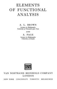
NONLINEAR CONTROL SERVO ACTUATOR
AIRCRAFT
GUST RESPONSE TRANSFER FUNCTION
GUST DISTURBANCECONTROL SURFACE
-I
-
+
:
RIGID BODY TRANSFER FUNCTION
;
:
STRUCTURAL RESPONSE TRANSFER FUNCTION
: RESPONSE :
...
-
RIGID BODY RESPONSE
+
: STRUCTURAL
...............................,
--
I
MEASURED SIGNALS
-FLIGHT
Figure A.
DYNAMIC RESPONSE VARIABLES
CONDITION VARIABLES
IDEAL MEASUREMENT SENSORS
4
+
;
AIR-DATA COMPUTER
I
Functional Block Diagram of the Aircraft, Control Servo Actuator and Measurement Dynamics.
1
--
-
A. V. 'Balakrishnan
NOMENCLATURE pilot command input force, lbs.
*s
acceleration due to gravity constant, ft/sec 2
g
2
Gw
angle-of-attnck calibration coefficient
Ka
M
Mach number
e
n
z
gust power spectral density (ftlsec) sec.
Dimensional pitch moment coefficients
normal acceleration, "g' s"-
9
dynamic pressure, lbs/ft
v
true velocity, ft/sec
w
g
2
incremental vertical.velocity due to air gusts, ft/eec
z
distance from c. g. to accelerometer, .ft.
=a
Dimensional normal force coefficients
'6
e
a
.angle-of-attack, rad
ir (sub) distance from c. g. to angle-of-attack vane, ft.
'e
elevator deflection angle, rad
A. V. Balakrishnan
NOMENCLATURE (Continued) commanded elevator deflection angle, rad pilot command input deflection, inches damping ratio of the jth bending mode pitch attitude, rad slope of the jth bendingmode at angle-of-attack $me, rad/ft slope of the jth bending mode at pitch attitude and rate sensor, rad / ft displacemenr of the jth bending mode at reference station, ft relative displacement of the jth bending mode at the accelerometer forcing function coefficient % r bending modes, ftfsec
2
characteristic frequency of gust power spectral density, rad /sec natural frequency of the jth bending mode, rad/sec
A. V. Balakrishnan
Taking the state equation as:
x = Ax
+ Bu
x(0) = 0
we wish to find u(t) so a s to minimize:
where 6 (t) i s a unit step function. By the usual analysis, the optimal P , u(t), denoted uo(t) i s given by:
[The main point to note i s the appearance of
m
as the upper limit in
the integral.] We can express this solution alternately a s
u (t) = D
B* -Y(t)
O0
3 choi-
sir convenablement . Ou a l e : (1) (2)
-
L1algorithme consider* e s t de type ARROW-HURWICZ [I] Si on s a i t que
u E W , W Hilbert inclu dans V avec densite et
injection continue ( dlob W c V cV1cWt), on peut p r e n d r e pour S un operateur de dualite
de W + \V1
R. Glowinski On cherche
P2
SOUS
l a forme:
.Pz= PC
PI=? Utilisant
P
(5. 12) dans ( 5 . l l ) , il vient :
Mais : ZC(1-P) si
p
0
0
( destine B tendre v e r s z e r o ) , on
definit successivement : (6. 5)
Rh = [ M . 1J
(6.6)
0.. 1J
I Mij E R2
=I 5 , xi
-
1 . q + J (resp. C.. 2 -1 ) 1 -
a
2
o x ( r e s p .oy).
1J
2
xi +
.
M.. = (xi. Y . ) x . ~=ih
J
1.l
ki
z [x]
= translate de
yj
h
- 5 ,
+ h- 2
y. +
J
. Y.J
=jh . i , j r Z I
[
de 4 . , parallelement 1J
R. Glowinski
4
e t on notera
qj, la valeur approchee
en M.. ; mdme rotation avec 1J
Pour dBfinir la variable duale
(du moins on ltesp&re) de u
f . . pour f. On posera: 1J
2 p ( E (L
2 (a) ) ),
il est commode d1in-
troduire un reseau Qh, de pas h Bgalement, decal6 par rapport R h de l a fason indiquee s u r la figure
6. 1 :
On utilisera systematiquement l e s relations 1
-1 j+
et
2 2 1 2 p 2 ( P = ( P , P 1) en
h
+
1 Z
et
2
Pi+
prendre
Mi+
, Pi + 1 . 1 pour les valeurs tfapproch6estl de p = ~ + ~
en compte
Mi+l j+ ; l e s points M ~ + L.+ 1 a 2 2 2 J Z sont ceux qui sont centre dlun c a r r e de cote
(v. figure 6. 1) dont un sommet au moins appartient B Roh
notera
!2 l h
-
1
llensemble de c e s points; on posera Bgalement :
et on
R. Glowinski Dans c e s conditions llalgorithme (6. 2) e s t
(p u
approch6If p a r :
donne n+ 1 i+ij
+
n+ 1 i-ij
u
,n+l
+
u.. ij+l
n+l 1
+
-
4un+1 -i j-
n g Dij Ph 'fij
(MijQaoh)
avec : Dij
1n Pi+-1 j+L 2 2
-
n
Ph
-
(6. 12)
+
1n
-
2n 1 1 P i+- j+ 2 2
-
1n
j+L
pi-L 2
2
+
P i+L 2
2h 2n 1 . 1 + pi+- J-2 2 2h
In
j-L2 -
2n pi-L 2
approchant
j+L
u
=
n+ 1 u. i+lj+l
-
2
AU
;S;;
n+l
'
au bSf
en Mi+L
2
J
j+L2
u n+l 2+lj 2h
9
+
n+l q+l
u..
2n
j+l- p . 1 . 1 2 1-5 J-2
approchant d i v p e n Mij,
2 Gi+L 2
pi+L j-- 1 2 +
- u .n+l . 13
R. Glowinski
(6. 14)
{
avec
n+ 1 Dans (6. 11, (6. 13), on convient de prendre u k l = 0 s i Mkl
4 nOh
On demontre dans CEA-GLOWINSKI [l] ,GLOWINSKI-LIONS-TREMOLIERES
[I] que (6. 11) , (6. 12), (6. 13), (6. 14) correspond 5 l1appli-
cation de llalgorithme
du
N. 4 (llalgorithme dlUZAWA)B 'la minimiJh (vh), convexe, non differentiable, en
sation dlune fonctionnelle
dimension finie ; J h Btant une approximation de l a fonctionelle problgme
du
(6. I ) , explicitee dans l e deux references ci-avant ; on y
demontre egalement la convergence de (6. 11) pour En ce qui concerne l a convergence de u h
-+
pn -
A)=
Min v,p
$(v,p;A)
Min [(Av.v) - 2 ( f , v ) + 2 A l l v l l I - ~ 2 ] v
d'od :
(1)
Ce
e s t B distinguer de celui de la r e m a r q u e
7. 1.
'R. Glowinski Min J (v) = Max v X I
Min
= Max
+
-
2 Al/v
Min [ ( A v , ~ )- 2(f.v) + 2(t,v)-
Max
= Max
(7. 17)
[(Av,~; ) 2(f,v)
v
1
2 Max ! A V , V ) - ~ ( ~ , V ) + ~ (h~ , V ) 4JlltIlrn5A
Min
t = Max
Min v
t
]
2
[(Av,v)-2(fJv)+2(t,v)-
1ti/
2
Mais
Min [(Av,v)- 2(f,v) + 2(t,v)] = -(A-'(f-t) , (f-t) ) v - 1 f l a formulation du probleme dual d'oG posant g = A (7. 18) Min t
[(A-' t , t )
-
2 (g, t ) +
la fonctionnelle J* (t) = (A-I t, t )
-
~(tll 2(g, t )
+
11 ti1
2
e s t non differen-
tiable et l'utilisation d'une m5thode de gradient s u r l e probl&me dual (7. 18) conduit A des difficult& lies A l a non differentiabilite de t+\l t/j
'
m
8. Un probleme de contrsle optimal ------ avec fonction cout s n differentiable Soit R un ouvert borne de R Q =
n X ] O , T [ ( T fi")
on s e donne
,
n
2
de fronti@re =
r
x ] 0, T
suffisemment r e g d i e r e et
C;
:
I
Y ( x , O ) = yo (x) dans R
G. Glowinski avec
I E L~ (Q) , y o E L~ (Q). 1 L e contr6le v &ant donne, (8. 2) admet une solution unique dans H (Q),
soit
y (v)
(8.3) avec o(
, et on peut definir l a fonction co3t
J(v) =
>
o
(QIy(v)
-jd12dxdt+dL
:
1vl2dxdt
zrhlvla
. /j > o e t a E L 2 (Q).
I1 r e s u l t e de
LIONS [I]
que l e probleme :
Min J ( v) vEUad adrnet une solution unique , soit Compte
u , qui e s t l e contrzle optimal.
tenu de LIONS , loc. c i t . , et des N. 2 e t 3 , on montrerait
facilement llexistence et lrunicite de p. p. s u r Q solution de At
f
=
+ u
sur
y (x,t) = o y (x,o) = y
P (x,t)
=
0
sur sur >
R
~
p. p . sur
Q I1
u 20
IXI Xu
x O] , T [
sur R
(x)
o
+PA+p
(du
~
s u r x
p(r,T)=o o(u
avec
:
'Y - b y (8. 5)
( y,p, u,X)
11
1
+PA+p ) u =
1.1
= 0
It 11
I
X(x t ) ( 1~
dt
R. Glowinski Reciproquement
si
(y,p, u,
1)
e s t solution de (8.5), (8. 6), (8.7) u
e s t contr8le optimal. L1utilisation de (8.5), (8.6), (8.7), associee B des algorithmes du type de ceuxdeveloppes
aux
N. 4 et 5 , a donne des resultats nume-
riques satisfaisants pour l e probleme (8.4) , mzme pour des valeurs assez petites de o(.
: 9.:
Une remarque s u r l e comportement des mulSiplicateurs de Lagrange. I1 a souvent Cte constate que, la fonctionnelle J
ficacite des methodes duales etait une fonction
I1
&ant donnee, l1ef-
(en particulier celles des N. 4 et 5 )
..
decroissantell
du convexe K, ceci. n l a rien de
t r 6 s surprenant puisqu1.5 la limite lorsque K s e reduit B un point l e problkme dloptimisation considCrC de Lagrange en gGn6ral.
n'admet pas de multiplicateurs
On. va mettre ce phenomeme en evidence s u r
un exemple t r e s simple :
V
Soit
=
R
, J definie par
On prend pour K E l e convexe &ant donnee par :
D1o~ le Lagrangien :
La solution optimale de
(9.4)
Min y(K
6
J (y)
[y
:
1 1 y 15€1 , llappartenance
K
E
R. Glowinski e s t donnee de fa$on 6vidente p a r :
(9.5)
ye
=
min
e t l e multiplicateur
( 1 , E )
de Lagrange
E
de : (9.6)
d'ofi :
Min J ( y ) YEKE
=Min&(y.a)
Y a
correspondant s'obtient & p a r t i r
-
R. Glowinski
B I B L I O G R A F H I E ARROW K. J. - HURWICZ L. [I]
CEA J.
CEA J.
- GLOWINSKI
-
R.
GLOWINSKI R. Li]
NEDELEC J. C. -
DUVAUT G.
-
[l]
-
LIONS J. L.
GLOWINSKI R.
: Dans Arrow-Hurwicz-Uzawa,
Studies i n l i n e a r and non l i n e a r programming. - Stanford Univers i t y P r e s s 1958. : MBthodes numeriques pour llecou-
lement l a m i n a i r e d t u n fluide rigide visco-plastique incompressible A b a r s t r e - (R~DDOI-t IRIl\ d i s ~ o n i b l e ) : Methodes duales pour l a minimisa-
tion de fonctionnelles non diffkrentiables - A p a r a i t r e dans l e s p r o ceedings d u Colloque d'analyse numCrique de DUNDEE- 197 1, SPRINGER VERLAG. : L e s inequations e n mecanique et en
physique
[I]
-
DUNOD 1971
: Methodes Numerique pour llCcoule-
ment stationnaire d l u n fluide rigide visco-plastique incompressible Proceedings of the 2. nd. Int. Conf. on Num. Methods i n Fluid DynamicsL e c t u r e Notes i n physics, 8 , Springer - V e r l a g 197 1 : Expose B cette reunion CIME c z -
s a c r e B llAnalyse NumCrique du ProblPme e l a s t o - ~ l a s t i a u e . GLOWINSKI- LIONSTREMOLIERES.
GOURSAT
5
C1l
: L i v r e s u r llAnalyse NumCrique des inequations variationnelles, 5 parai-
t r e an 1972 chez DUNOD : A.nalyse Numerique d e problemes
dlelasto-plasticit6 e t de visco-plasticttk. - T h e s e de 3 cycle PARIS-IRIA, 1971
R. Glowinski KY-FAN
[I]
LIONS J. L.
MOSCO U.
S u r un t h e o r e m e de Min Max C. R. A. S. - P a r i s , 259, 39253928, P a r i s .
:
[I]
[l]
Controle optimal de s y s t e m e s g o u ~ e r n e sp a r d e s equations aux derivees p a r t i c e l l e s - DUNODGAUTHIER-vILLARs 1968
:
Expose 5 cette reunion CIME
:
ROCKAFELLAR R. T.
[I]
:
Convex Analysis P r e s s 1970
-
Princeton Univ.
SION M.
C11
:
On g e n e r a l m i n max t h e o r e m s Pacific J. Math. 8,1958, 171- 176.
UZAWA -- H.
El]
:
Dans ARROW- HURWICZ-UZAWA. loc. cit.
C E N T R O INTERNAZIONALE MATEMATICO ESTIVO ( C . I. M . E . )
J. L . LIONS
Corso
tenuto
ad E r i c e
dal
21
g i u g n o a1 7 l u g l i o
1971
.
APPROXIMATION NU~ERIQUEDES INEQUATIONS D '~VOLUTION J.L. LIONS (Paris)
Introduction.-
On donne dans ce cours les methodes fondg
mentales pourla r6solution numerique des inequations d'Svolution intervenant en Mecanique et en Physique. ~exSexperiencesnumerique, faites
a 1'I.R.I.A.
(Paris),
i
seront present&
avec toues les details dans un livre de R.
Glowinski, R. TrbmoliSres et l'A., a paraitre chez Dunod.
Plan detaill6. CHAPITRE 1 . 1
Inequations d'evolutions parabolique. Type I.
. Exemples .
2. Formulation generale. 3. Solutions fortes et faibles. 4 . Generalitgs sur les methodes constructives d'approxi-
mation. 4.1
Reduction 5 un equation parabolique. Penalisation.
4.2
Reduction 5 un equation parabolique. REgularisation.
4.3
Reduction 5 un inequation elliptique. Regularisation elliptique.
a un inequation elliptique. Discr6tisation.
4.4
Reduction
4.5
InQquation d'6volution et points selles.
J.L. Lions
CHAPITRE -2.
-
Approximation par discretisation des inequations paraboliques de type I.
1. Approximation d'un couple d'espaces. Constante de stabilit6. 2. Schemas d 'approximation 'des inequations paraboliques de
type I. 3 . Analogue de la stabilite.
4. Etude de la,convergence.
CHAPITRE 3 . -
Inequations d'evolution paraboliques de type 11.
1. Exemples. 2. Formulation gQn6rale. 3.
Schemas d'approximation.
4 . Stabilite et convergence.
CHAPITRE 4. - Inequations d16volution du 2eme ordre en t. 1 . Exemples. 2. Formulation ggngrale. 3 . SchQmas d 'approximation.
4. Stabilite et convergence.
CHAPITRE 5.- Complgments et problSmes.
1. Ecoulement de fluides de Bingham. 2. ProblBmes ouverts.
BIBLIOGRAPHIE.
J.L.
Lions
CHAPITRE I.- I n e q u a t i o n s d ' e v o l u t i o n s p a r a b o l i q u 1.-
Exemples. Exemple 1 . 1 . -
La t h e o r i e d e l a d i f f u s i o n e n m i l i e u x p o r e u x
( c f . Duvaut-Lions Soit
n
[lj)
c o n d u i t 3 d e s problemes du t y p e s u i v a n t :
o u v e r t borne de R
(n=2
o u n=3 d a n s l e s a p p l i c a t i o n s ) d e fro; tiere
le 3
r
2
"r6guli&re8'. Soit
l a norma-
r dirigee vers l'exterieur de a.
On c h e r c h e une f o n c t i o n u = u ( x , t ) , xe 0, t>0, solution de (1.1)
aU at
[ , T>O f i n i q u e l c o n q u e ,
x ]O,T
n x ]0,T[),
(oii f e s t donnee d a n s (1.2)
n
au = f d a n s
avec l a c o n d i t i o n i n i t i a l e ~
~ ( ~ 1 =0 u) 0 ( x ) I
I
un donne d a n s
n
e t l e s c o n d i t i o n s aux l i m i t e s (uiO
sur
o:"
sur
u & = o
Z = P X ] O , T [ ,
z, surz
.
Remarque 1.1.Le probleme (1.1 )
,
(1.2)
,(1.3)
e s t non l i n e a i r e Z cause d e s
c o n d i t i o n s aux l i m i t e s ( 1 . 3 ) . Remarque 1.2.DtaprSs u = 0
sur
u
c0
c
an
z
= 0
sur Z,
on voit q u e
J.L. Lions
an
o
=
sur
Z-
zo.
Mais Zo n'est pas donne 3 priori. Orientation. Le but de ce premiGr chapitre est: a) de montrer brievement corn ment le probleme (1.1), (1.2) , (1.3) (et, a vrai dire, des problemes beaucoup plus gen6rauxJ. est bien pos6
(
1
1;
b) de donner des m6thodes d'approxirnation numerique de la solution du problsme. Donnons un 2eme exernple. Exemple 1.2. On cherche u satisfaisant 3 (1.1),(1.2) et aux conditions aux limites sue
I
(1.4)
u 32
+
glul =
Z
o
g constante sur z
>Or
.
an
Autrement dit:
On verra que ce probleme est encore bien pose.
1
( )
[I]
Pour une 6tude plus systgmatique de la theorie, cf. H B&ZIS J.L.
LIONS [lJ[2]
.
J.L. Lions
2. Formulation ggnerale. Nous donnous maintenant une formulation "abstraite" de pro blSmes dlinequat.ionsde type parabolique, puis nous montrons cog ment cette formulation contient, en particulier, les exemples du N.1. Soient V et X deux eispaces de Hilbert ( 1 ) (2.1)
VcH
,
sur E,avec
V dense dans H I l'injection de V dans H etant continue.
On designe par:
(2.2)
I
I I
la norme dans H,
(
,
)
le produit scalaire
correspondant dans :HI
II II
la norme dans V
D'aprGs (2.1), il existe une constante c>O telle que
On se donne ensuite: bilingaire continue sur V x V, coercive au sens: il existe X tel que Ivl
l2
, a>O, VV E V ,
et on se donne encore: (2.5)
K = ensemble.convexe ferme dans V;
(2.6)
j = fonction convexe continue de V +1R
.
On identifie H 3 son dual et l'on introduit l'espace V' dual de V
1
( )
On peut aller beaucoup plus loin, enprenant pour V un espace
de Banach reflexif. Cf. Lions [2]
et la bibliografie de ce livre.
J.L.. Lions
de s o r t e que (2.7) S i f E V'
, on
ddsigne p a r ( f , v ) son p r o d u i t s c a l a i r e avec v E V;
c e t t e n o t a t i o n e s t c o m p a t i b l e avec c e l l e du p r o d u i t s c a l a i r e dans H. Le problsme. 1 O n c h e r c h e une f o n c t i o n t + u ( t ) d e [o,T] + V ( ) t e l l e que (2.8)
9
u ( t ) E K,
Un a u t r e probleme est: On c h e r c h e u = u ( t ) d e [o,T] +V t e l l e que
'tlv E V r
avec ( 2 . 1 0 ) .
L ' i n d q u a t i o n (2.9) ou (2.11 ) e s t c e q u ' o n a p p e l l e r a i c i une inequation parabolique de type I Remarque 2.1
.
S i K=V ou s i j=O,
2
( )
1
( )
(2).
(2.9)
et
(2.11) s e r d d u i s a n t 3 l ' e q u a t i o n :
Cf. l e s i n d q u a t i o n s du t y p e I1 au Chap.3. Dont il f a u d r a p r e c i s s r l e s p r o p r i 5 t d s .
J.L. Lions
Remarque 2.2. Si la fonction v
+
j(v) est diffgrentiable sur V alors (2.11)
Bquiva~ita l'equation (en ggn6ral non lingaire): (2.13)
au(t) , v ) + a ( ~ ( t ) ~ v ) + ( j ~ ( ~ ( t ) ) , v ) = ( f ( t ) , v ) ,V V E V . ( at
Remarque 2.3. Introduisons A
E
$ (V;V' ) par
Alors (2.13) gquivaut 2
Remarque 2.4. Si l'on considere la fonction $k indicatrice de K 0
1
( ):
si v e K ,
JI (v)=
(2.16)
k
+msi
V#K
alors (2.8) (2.9) gquivaut 3 : (2.17)
au(t) ( , t , v-u(t) )+a(u(t) ,v-u(t) + ~ ~ ~ ( v ) - $ ~ ( u) (3 t )
Les ingquations (2.9) sont donc des cas particuliers de l8in&quation
1
( )
La fonction $k est convexe et semi continue infgrieqrement.
J.L. Lions
I
vvcv 1 09 y e s t une fonction convexe propre (cf. le cours de U. Mosco [I]).
Utilisant la notion de sous diffsrential, on voit que
(2.18) 6quivaut 3
equation parabolique multivoque. Exemple 2.1.Voyons comment 18enonc6 gen6ral recouvre le probleme de 18Exemple 1.1. On introduit (notations des cours de R. Glowinski et U. Mosco): 1
(2.20)
V = H (n),
(2.22)
a(u.v)=
2
H=L (n),
&.K dx i=
ax. ax. 1
1
Alors le probleme (2.81,(2.9) ,(2.10) 6quivaut au probleme (1.1),(1.2),(1.3). Exemple 2 . 2 . On prend V,H,a(u,v) c o m e en (2.20) ,(2.22) et 180n intro duit
Alors le probleme (2.11 ) , (2.10) Bquivaut au probleme (1.1 ) (1.2), (1.4).
,
J.L.
Lions
Origntation. On va m a i n t e n a n t p r g c i s 9 r 3 q u e l s e n s on e n t e n d l e s " s o l u t i o n s " ' d e s probl6mes p r g c g d e n t s .
3.-
Solutions f o r t e s e t faibles. Solutions fortes. Par " s o l u t i o n f o r t e " du problsrne ( 2 . 8 ) , ( 2 . 9 )
,(2.10)
on en-
t e n d r a une f o n c t i o n u t e l l e que
(3.3)
(3.4)
u(t)e K
I
p.p.
en t
(z pour
tout t E
[o,~])
s a u f p e u t S t r e pour t d a n s un ensemble Z c [o,T] de mesurenulle, ona:
e t naturellement (2.10) ( 2 ) :
Evidernment ( 3 . 3 )
3 impose ( )
( I ) L~ (0,T; X ) = e s p a c e d e s " f o n c t i o n s " t + u ( t ) d e T 2 mesurables e t telles que I I u ( t ) l l dt<m
jo
2
( )
[o,T] +X
qui sont
•
X
I1 r 6 s u l t e d e ( 3 . 1 ) e t ( 3 . 2 ) que t + u ( t ) e s t , a p r e s modifica-
t i o n 6 v e n t u e l l e s u r un ensemble d e mesure n u l l e , c o n t i n u e de [O,T] A l o r s u ( 0 ) a un s e n s . 3
( )
Tant que l ' o n t r a v a i l l e avec d e s s o l u t i o n s f o r t e s 06 ( 3 . 3 )
l i e u pour t o u t t .
a
+H.
J.L. Lions
I1 est important pour les applications d'lntroduire tion de solution faible
(cf. Lions-Stampacchia [I],
une no-
Brdzis [ z ] )
.
Pour simplifier l'expose nous prenons
On observe alors que si u est solution "forte1'de (3.4) , on a:.
[
I
,v-u)+a(u,v-u)-(f,v-u) dt50
(3. 8)
V V E L2 (0,T;V) tel
que =EL' at
(o,T,v') et v(t) 6, K p. p. et v(O)=O. '
Mais c o m e
n'intervient plus dans (3.8) on peut ddfinir u cop! at me solution faible si u satisfait 3 (3.1), (3.3) et (3.8). Remarque 3.1.On a 6videmment des notions analogues de solutions "fortes" et "faibles" relativement
3 11in6quation (2.11)
.
Remarque 3.2.Seuil de .c6gularitS. La solution u(t) des problemes prdcedents n'est pas une fonction "trGs r6guliSre8'de t, quelle que soit la rdgularit6 des donnes f et uo. Prenons en effet V=H= IR,
a (u,v)=O (qui v6rifie (2.4) lorsque V=H),
J.L. Lions
La solution est indiquee
sur
le graphe ci contre. On voit que, 2
en particulier,
at2
$
L' (0,T).
Resultats ggngraux. On demontre
1
( )
les resultats
suivants (cf. par ex. Lions [2]
et
L L 0
la bibliographie de ce travail):
-
>C
TheorSme 3.1.- On suppose f E L~(O,T;V'). On suppose que (2.4) a lieu. I1 existe alors une fonction u et un seule satisfaisant
a
(3.11,(3.31 ( 2 . 8 ) .
TheorSme 3.2.- On suppose que (2.4) a lieu et que
I1 existe alors un solution forte et une seule de (3.1). ..(3.5). Remarque 3.3.On a des enonci!s analogues pour l1ini!quation (2.11). Remarque 3.4. L'unicite des solutions fortes est immediate. Pour l'uniciti! des solutions faibles, si.ul et u2 sont deux solutions Bven-
tuelles, on introduit: 1
( )
Nous donnons ci aprPs guelques indications sur les methodes
'constructives possibles de dgmonstration et au Chap.2 nous donnons l'approximation numgrique de la solution (qui peut, d'ail-
J.L. Lions
1 W = -(u +u ) 2 1 2
et l'on prend v=w u1 et u2
,
puis w
e
solution de
dans chacun des inequations (3.8) relatives 2
E
.
On additionne et.on peut alors faire e
-+
0. Cf. H. Brezis
c21 4.- G6ngralit6s sur les m6thodes constructives d'approximation.
4.1.-
Reduction 2 une equation parabolique. penalisation.
Soit 6 un operateur de penalisation attach6 a K (cf. Lions [2], p.370 et les cours de R. Glowinski et U. Mosco). On
"approche"
(3.4) par 1 "equation penalisee (4.1)
au ( 7 ,v)+a(u
1
(t),v)+;(~(u~(t)),v)=(f(t),v)
VVGV,
E
oil
E>O est destine 2 tendre vers 0, avec
--
I1 s'agit d'un probleme parabolique non lin6aire monotone (car 6 est, par definition, monotone de V
-+
V') dont on sait qu'il
admet une solution unique. On montre (Lions [2)) Theoreme 3.1
,-u E
que, par ex. sous les conditions du 2
-+
u dans L ( 0 , T ; V )
faible lorsque
.
E-+Ooh u est
solution faible. On peut ensuite approcher ur par l'une des msthodes de reso
J.L. Lions
4.2.- RPduction,&un equation pbrabolique. R6gularisation. Dans le cas. des inequations (2.11) on peut introduire j (v), EI
approchant j ( v ) . Par ex.
fonctionnelle convexe differentiable
,
dr
o
on prendra
est convexe, differentiable, et par exemple
y
(X)=IXI E
si
\ A ( > E
On "approchet'alors (2.11) par llequation rggularisee %u (4.3)
,
(* v)+a(uE,v)+(j~(u
avec (4.2)
,v)=(C,v)
Vv E V I
E
.
11 s1agit 12 encore d'une gquation parabolique non lineaire monotone
2
et on verifie encore gue u
-+
u dans L (0,T;V) faible,
u solution faible.
4.3.- Reduction 2 un inequation elliptique. Regularisation elliptique. Pour reduire par ex. (3.8)
a un situation
d e j a connue, nous
nous somrnes rarnenks jusqtici 2 des equations dlBvolution. On peut essajer de se ramener 2 des inequations stationnaires. pour cela, on considere le probleme de nature elliptique: trou ver u
fi
oii
fGo =
{v
E E
(4.4)
I
2 av veL (O,T;V), % E L
2
(0,T;H),v(t) E K v(O)=O>
solution de
1
P.P. I
J.L. Lions
Cette inequation entre dans le cadre de inequations variationnelles-elliptiques etudiees dans le cours de R. Glowinski et U.
= .
MOSCO 7 ( 1 )
On montre (cf. Lions-Stampacchia [I] u
par ,ex.) 1 'existence de
solution de (4.5) et la convergence de u
vers la solution E
faible lorsque Remarque 4.1
E
+
0.
.-
On peut utiliser pour llapproximation de la solution u
€
de
(4.5) les methodes descours Glowinski et Mosco. I1 est possible (mais non encore verifie sur des exemples num6riques)que l'usage de (4.5) soit utile
pour des calculs sur de longs intervalles
de temps. Cf. Carasso [I] pour le cas .de equations. Remarque 4.2.On peut utilis6r simultanim_ep~le5 id6es de 4.1 on 4.2 et 4.3. On peut donc se ramener 3 des equations stationnaires.
4.4.- Reduction 3 une inequation elliptique. Discretisation. La methode peut Gtre la plus naturelle de reduction au cas
(
1
On notera que le probleme (4.5) est non symetrique meme si
l'on part dlune forme a(u,v) sym6trique.
J.L. Lions
elliptique est dlutilis&r la discretisation de la deride en t. En raison de l'importance essentielle de ce procede pour les applications numBriques, nous etudions cela en detail au Chap. 2..
4.5.- InBquations dl&volution et points selles (cf. Tremolieres C11 1
. On introduit
et 1 'ensemble
On vBrifie que si u est solution forte alors
autrement dit: {u,u} est point selle de L(v,w) .
sur
hxh.
A
RBciproquement, soit {u,u) point selle de L(u,w) sur & x X , Alors (4.9)
L(u,w)
L(u,Q) 4 L(v,Q)
vv,w ~
3 d
d l o a l1on deduit (en observant que ~ ( u , u=L ) (QIQ)=0) que L (u,Q)=O. Alors L ( v , ~>o )
et
L(w,u)=-L(U,W) a0
donc dlaprSs 11unicit6 dans le Theoreme 3.1 (ou 3.2) on a: U
= u.
J.L. Lions
Donc
u est solution, alors {u,u) est point selle de
L(v,w) sur
Kx k
et rgciproquement.
On peut dgduire de 13 une mgthode de demonstration de l'&stence de solutions. En effet si K est born6 dans V, alorsk est born& dans l'espace W des fonctions v 6 L~ (0,T;V) avec
E L ' (O,T;Vt)et l'existence at d'un point selle (ngcessairement de la forme {u,u}) est consGqueg
ce d'un resultat classique di Von Neumann. Si K n'est pas borne, on i n t r ~ d u i t ~ KR =
CV I v
E
Kt
1 lvl 1
6 R};
soit uR la solution de
Prenant dans (4.10 (4.11)
J
:
I luRI I 2dt
v=O on en d6duit que
lid inf
[$
laN-l
12+
1 N-1 7 a(u 1
-
1 !w'(o)
-'1
TI
a(w(o))
J.L. Lions
de sorte que
pour toute fonction v par exemple continue de [o,T]
+
K
-
et
par prolongement par continuite, t/v E L~ (0,T;V) avec v (t)E K P -P. On ddduit de I3 que w=u=solution du 'problSme, d'oO le TheorSme sous reserve de la verification de (4.29)
.
Mais
d'oO le resultat dlaprSs (4.5). Remarque 4.1. Les resultats pour le schema (3.9) sont tout 3 fait analogues aux precedents. Faisant v=O dans (3.9) on en deduit: (4.32)
(
6"-6"-1 At
,6n)+a(un,6n)~(fn,6n 1 .
Mais a(un ,6n )=a(un+l , 6n)-~ta(6") d'oii en portant dans (4.32) et en multipliant par At:
J.L. Lions
Par sommation on en deduit
d'oil l'on dgduit, &
1 6"1 '+a(~"+~)
0 , that for each function &f) the
relations hold
( A Y . 9 ) L f ( y . y ) >o, being different from
(1. 3)
0 and for the sake of simplicity i s defined
G . I. Marchuk by A
> 0.
The operator A is called positive semidefinite if there a r e
such non-trivial
0E
,elements which turn the inner product (A lp, rp )
into zero. For a l l the remaining elements there holds the inequality
Below we shall formally denote positive semi-definite operators byA > 0. Let u s introduce then an adjoint operator A*, satisfying the Lagrange identity (Ag, h ) = ( g , A* h ) .
4 and h E 4. The space 4*, generally coincide with 4 ,though the domain. D of definition
If i s essential to note that speaking, does not
(1.5)
g E
of basic and adjoint functions is the same. To clarify the fact we shall show that
in many problems of mathematical physics
longing to the Hilbert space
@
g - function be-
satisfy some homogeneous boundary
conditions. In the application of the Lagrange identity (1. >), a s a rule, alongside with the operator
* those
boundary conditions which a r e
A
satisfied by the adjoint functions
h
a r e defined.
Further, we shall
apply a more convenient notation for adjoint functions. Thus, if the elements of the space of functions
* @ are
adjoint space
denoted by (P , then those of the
suitably denoted by
In the case of A Then
(Z, a r e
= A*
q=@.
CP*
, the operator A is called self-adjoint.
Note an important consequence connected with the properties'of the adjoint operators. it follows that Fourier
-
A*
>
Thus, if A
>
0
, then from the Lagrange identity
0.
s e r i e s expansions by eigenfunctions of basic and adjoint
operators a r e of great importance f o r the analysis of algorithms.
G. I. Marchuk Consider the two following spectral problems for A
Assume that each of the homogeneous equations forms a complete set of orthogonal eigenfunctions {u
n
2
0:
(1. 6) , (1. 7) and {u*), which n
can be normalized a s follows:
and eigenvalues
n
belong to the interval
We shall call this complete set of eigenfunctions a biorthogonal basis. Then supposing completeness, any flinction f of
@
and f*of @*can be r e -
presented a s a Fourier s e r i e s
where
Later we shall consider, without stipulating, the spectrum of
A
>0
and
A
-> 0
operators to be real. Hence, it is not difficult to A A establish that in such a case 1 > 0 and 2 2 0. n n Of great value for the analysis of numerical algorithms a r e esti1
2
mations of norms of operators. The norm of the operator from :
A is definyd
G. I. Marehuk
(further f o r the sake of simplicity the restriction
#
(fl
0 will not be stated).
A
Taking into consideration the relation
tlie'squared norm of the operator A can be also written a s follows;
ll 2 The operator
* A A is
=
sup
('p , A * A ~
(rp.9)
cp€+
symmetric and positive sani-definite. Consider
a spectral problem
A*AR =
X~
*
(1. 13)
The problem defines a s e t of eigenfunctions
bJ
X A * ~ > 0. The set n any function yY of
@J and
eigenvalues
for symmetric operators is complete. Then
Q A Acan be
represented a s a F o u r i e r s e r i e s
where
cpn Substitute the s e r i e s tion
R
n
=
((P
.nn).
(1. 15)
(1. 14) into (1. 12) and u s e the condition f o r func-
orthonormalization. Then we shall have
where Q is a Hilbert space of F o u r i e r coefficients. It is not difficult to find that
-
11
1
;
11
XA'A
min
;
d
A*A '
G. I. Marchuk
where
A* A Amin
and
A*A max
a r e minimum and maximum eigenvalues
respectively from the totality hAtA of the spectral problem (1. 13). n A*A The value is usually called a spectral radius of PA*A = max the ,dperator A*A. li
9
In the case of a self-adjoint operator A consider
problem. Au = We have
IIAII
=
xA
u
a spectral
.
(1. 18)
FA-
If i s evident that for the self-adjoint operator
Let us consider certain properties of norms of operators
the problem
of eigenvalues. 1. 1. 1. Energy Norms. Later we shall always deal with Hilbert spaces of real functions with the norm (1.21) where C
> 0 . It
is easy to see that using the Lagrange identity we have
the equality
and consequently
C+C* 2
The operator C
i s symmetric and positive. It means that i f
> 0, then the norm of lp function can always
be presented a s any
inner product with a symmetric operator in the form of the weight function, i. e.
.
On the basis of Buniakowsky-Schwarz inequality
one can obtain the following important estimation :
where
dC+p and
-2
-
i s a maximum and minimum eigenvalue of
2
the symmetric operator
c + c" , 2
F o r simpler and more frequent cases one usually assumes C = E. Then we get
1. 1. 2.
Estimation of the Norm of a single operator
Let us consider a positive semi-definite operator A
2
0.
There
is the following relation :
II(E
+&A )-l11< 1
(1. 25)
for any parameter 6' > 0. This assumption can be proved by the formula
G. I. Marchuk
11
( E + @A)-
1
(1 =
( (E + ~ A )- l q ,(E + ~ A ) - l q
sup
26)
( Y W
Let u s take
y,
=
(E
+
G-~)-lq
a s a new t r i a l function of (1. 26). Then we get
11 ( E
As A
A
->
>0 ,
-
('t'>Y')
( ( E + C A ) (I, , ( E + C A )
0,
=
)
the estimation (1. 2 5 ) follows f r o m the l a s t relation. If
we have
1. 1. 3. If
-
+ W A ) - ' I ~ = sup
Kellogg's Lem= A > 0 and
>
0
, then
Let u s introduce the notation
T = ( E - r A ) ( E + #A)Consider t h e expression f o r
I( T I(
1
G . I. Marchuk = sup
( ( E - ~ A ) ( v (, E - W A ) ( Y )
-
y E \ Y ((E+O-A)Y, ( E + c A ) y ) = sup YIEY
(yJ, W )
-2
(A yr,
( y , y)+2 (Ay,
2
'Y )+a( A Y s A ' ? )
0
instead of (1. 28) we shall get
1. 1. 4. Estimation of the Norm of Operators A.s it was stated above
Since the squared norm of the operator A coincides with the spectral radius of the self-adjoint operator A*A, to define/3A,A
one can use the well-known
iterative Kelloggls process, i f A i s a normal operator, that ,is AA*= A*A,
where index k denotes the number of the sequential iteration of the following scheme :
The proof of the convergence of the iterative process (1.29)imme-
-
G. I. Marchuk
diately follows from the Fourier analysis. In.fact, let
where the
R a r e eigenvalues of problem (1. 13). Consequently n
Substituting the series into' (1.29) with large k we have
Am
where
=/$I*A
=
11 ~ 1 a n1 d 1~;-
is the eigenvalue preceeding '
its maximum of the operator A*A. 1. 1. 5. Cdculation of Spectrum Bounds .of a Positive Matrix Consider a problem of finding out maximum and minimum eigen~ a l u e sof the operator A, havifig a positive spectrum Au=
A
u.
F o r this purpose we use Lyusternik's method. We shall introduce an iterative process
where c
is a normalization factor, which i s conveniently chosen in n (n) the form c . Them n
=11~
9
= A
$111
and
/A
= lim
n+m
1,
y(n)
11
1
G. I. Marchuk Here the following norm i s used
where
a r e vector
selected to the order
y(n) components. The constant c
PA.
Then consider the matrix
B
n
i s usually
= / j A- ~ A
and the problem
It is evident that
B.2
0. Then consider again Lyusternikts iterative
process
and get
It i s easy to s e e that operators A and B have a common base and
Hence
=A-A.
Un this way not only maximum, but also minimum eigenvalues bf the matrix A a r e found. We assumed the matrix A to be of the form in which Lyusternikts method is applicable. 1. 1. 6. Examples Let us now go over the simplest examples which later will help illustrate methods i n numerical mathematics.
G. I. Marchuk 1. Let
where
A=
3 3;2
p 32
+
is the Laplace operator. The operator A
is defined on a set of r e a l functions
+,
whose elements satisfy the fol-
lowing requirements. B r s t ,
where 3 D is the boundary of the domain D. F o r the sake of simplicity it is assumed that the domain D i s a unit square Second , the functions
((P)
form a
{0 5r5
1, O
0.
At last, consider a spectral problem A
h
u
u = 0
=
Xu
in^,
for B D h .
The components of the eigenvectors corresponding t o (1. 56) u k1 = mP In (1. 57) the indices m
and
follows
sin
k m X h s i n lp7s h.
k, 1 specify the components
p a r e the numbers of eigenvalues :
are (1.'57)
of the solution, and
which can be ordered a s
G. I. Marchuk
uk1 mP
=
U
!
l , (i = 1.2 . . . . 1.
J
With the obvious relations
- A k (vksin
4
k r n ~ h =)
-a,ol s i n (
l
p h ~) =
sin
h2 4
h2
sin2
----mxh sin krnKh, 2 sin
i p h,~
2
the eigen-values will be = -4
mp Note that
Here the
m
and
1. a r e
p
mrch ---
( sin
h2
change from
ordered
mP
.
+
2
I to
pxh sin2 -1.
n-1.
As, usually ,
2
(1. 58)
Consequently,
*h 2
< 1 we can
write approximately sin2 7Ch --2
-
-- + n2h2 4
0
(h4)
hence , we get
Thus, we can write
The basis of eigen-vectors
(1. 57) can be used to present the vector
G. I. Marchuk a s a series
CQ kl
.
Then we get
where
The examples considered above give the necessary understanding of some operators and their properties.
-1.-2.
Approximation -----
Let us consider a certain problem of mathematical physics in the operator
where Here
form
cq
A is linear operator,
4
and
elements in
F
E
4
and
f E F.
a r e Hilbert spaces with the domains of definition of
D + 3 D and D respectively;
is
a linear operator of the
bountary condition, g e G , G is a Hilbert space of functions with the definition domain 3 D . Along with the equation (2. 1) , let us consider a s i m i l a r equation in a finite-dimensional euclidean space
a
'f
=
P,
=
gh
in
D~
, f o r aD,
G . I. Marchuk h where is a linear operator depending on the m ~ s h s i z e h , +h h f E F h , and. $h and F a r e euclidean spaces with the domain of h + a D h and Dh , respectively. Here Dh definition of elements D h
,y
is a set of inner
mesh-points of the D domain, and
3 D is a s e t of h the meshpoints, on which the boundary condition of the problem is aph proximated, ah is a linear ?perator on the grid g E G G is an h' h euclidean space of the vectors with the domain of definition a D h' Let us introduce the Hilbert norm of the vector i n grid spaces Fh,
Gh ,
.
Then we s h a l l denote by (
) the totality of values 7.h of any function of problem (2. '1) after projection on the grid domain
3 D o r Dh + aDh . Then the following definition is usually used.: h problem ( 2 . 2 ) approximates problem ( 2 . 1) with the o r d e r hn for the
Dh,
solution
where
cp
, if
M. a r e some constants different from
ca
.
F o r the cases where the solution of problem (2. 1) is
smooth
enough, e r r o r s in approximation a r e conveniently measured by the maximum norm peculiar t o the space of continuous and differentiable functions. To this end the Taylor-series functions participating in the formulation of the problem is used.
G. I. Marchuk L a t e r we shall assume that redtction of problem (2. 1) t o (2. 2) is made and moreover, the boundary condition of (2. 2) is used to eli-
minate the solution in boundary points of the
Dh
+ a D domain. As h
a result we have a n equivalent problem
h . is now the domain of definition of the solution D The soh' lution iph in boundary points is t o be found after solving equation
where
(2. 4) a s a result of a solution of
Eq. (2. 2)
with respect to the un-
knowns. Thus, in s o m e cases it is convenient to u s e form (2. 4) in writing an approximation problem, and in others form (2. 2) is
m o r e proper.
So, a s a result of the reduction applied with certain approximation, a problem with a continuous argument (2. 1) is reduced t o a problem in linear algebra (2. 4). F u r t h e r task is to solve a system of algebraic equations.
E x a m p 1 e.
Consider problems
The domain of definition D is assumed to be a square €0
5x 5
1 , 0
5
y
5
1 1 , and f
square D with a uniform grid along
-
a smooth function. Let u s cover
x and y
with m e s h s i z e h. The
mesh-points of the domain will be denoted by two indices (k, l ) , where the f o r m e r 3 0)
corresponding
to the spectral problem Au
=
Xu.
Introduce the following F o u r i e r s e r i e s :
where
u" a r e eigenfunctions of the adjoint spectral problem. Substitute (3.2) n into (3. 1) and multiply the result scalarly by u: . Then , if 7 > 0 we get expressions
Supposing that
f o r Fourier coefficients
G. I. Marchuk
we obtain the initial condition
The solution of ( 3 . 3 ) , ( 3 . 4) is obtained f r o m r e c u r r e n t elimination of the unknowns. A s a r e s u l t . we have
where r
n
=
1
-
7Xn.
Equality ( 3 . 5) is estimated
in modulus
We reinforce the l a t t e r substituting have
max J
I f h 1 f o r 1 fi- 1 I .
Then we
where
l fn l
rnax j
John Neumann introduced a so-called spectral critetion of stability.
It means that if f o r each harmonic
va
G. I. Marchuk
of the Fourier s e r i e s of ( 3 . 2 ) ,
t h e r e holds the relation
.1'
where C
C
2 -
a r e constants. independent of
j, then the difference
scheme' ( 3 . 1) is announced to be numerically stable. i ~ e u ts s e e what conditions should be applied to the p a r a m e t e r s of the difference scheme ( 2 . 12) to satisfy relation ( 3 . 8): Relation ( 3 . 7) analysis shows that sta-
bility criterion ( 3 . 8 ) is fulfilled if the condition
is imposed upon the parameter
r
.
n Suppose that the spectrum of the operstor
A
is situated in the
interval 0
0
.
Now let us come to a more general definition of the notion of numerical stability. ,For this purpose l e t us consider the problem
which i s approximated by the difference problem
G. I. Marchuk
We s a y that the difference scheme (3. 15) is stable , if with the fixed parameter
h , characterizing the difference approximation, t h e r e holds
the following relation for any
where the
h C1 , and
C:
j :
constants a r e independent of j.
The definition of numerical stability involves notion of the correctness of problems .with continuous argument. One can s a y that num e r i c a l stability establishes a continuous dependence of the solution on the input data for the problems of discrete argument. In fact , we choose, a s the input data of ( 3 . 15) f = f,,
and
g = g*
.
We get some solution of ( 3 . 15) and denote it by (4+. the input data
Then f o r the difference of the solutions
we have the following problem :
Then the stability condition becomes
Then we take a s
correspond
Hence it follows that small variations uf the solution t o those of the input data
f
and
g
.
It i s easy to s e e that the definition of stability a s it is given in
(3. 16) already relates the solution itself with a priori information
of the input of the problem. Such a definition i s more convenient for stability Bnalysis of many prqblems than the one due to Neumann. Let us consider stability of (2. 12) from this point of view., To this end we rewrite
the recurrent relation (3. 1) a s
where
The formal solution of (3. 17) i s
We shall estimate solution
(2. 28) by the norm using the Cauchy-Bunia-
kowski inequality and the triangle inequality.
We replace
11 f j - I 11
by the maximal value in all
Let
max j Then
Then we get
Il ll = I II fJ
j
.
If we put
then scheme
(2. 12) will be stable in the sense of the definition (3. 16).
It i s natural that condition (3. 22) is a sufficient condition of stability. One could get finer and weaker criteria through the norms of the powers i of the step operators 11 T )[ (i = 1,2,. ,j). However, such a weakin-
..
ing of the condition makes difficult a constructive procedure for establishing the stability criterion.
A s a rule , in practical calculations the sufficient
condition of
the form (3.22) i s usually applied.
A =A'>
Let us consider a case with the operator
0
and denote
Then
Let
'f=z
n
where
(u,)
~
~
n
~
n
'
is the base of the operator A .
Then
J
=
1
- 2 t X + -c2
2,
where
Let us find conditions to be satisfied by 7
, s o that J < - 1 ,
i. e.
then
H e n c e , if
P A =l l h ]
mar
=
An
=
,then 1.
We get following sdficient condition of stability :
Z
.
0 ,already independent of h, i. e. C l = max h
ch 1
and
C2 =
max h
Thus,with the constructive approach to the establishment of stability of some o r other difference scheme it is always preferrable to h h define C1 and C constants f o r h fixed. However, i n the c a s e s when 2 passages to the limit a r e studied with h + 0 , Z+ 0 , judgement of '
stability should be connected with either of
h
o r of
Z
.
C1 and C2
constants independent
It i s this view of stability that we shall use
in the investigation of the convergence of approximate problem solutions to accurate ones, with simultaneous tendency of
h and Z towards zero.
A s i m i l a r consideration r e f e r s to the definition of numerical stability in the f o r m (3. 3 1).
-- 1 . Let us investigate the numerical stability of differenExample ce schemes approximating the equation of heat conductivity. In the c a s e of an explicit scheme (2. 21) we had the norm of the step operator in the form (2. 28)
Now let
(1 T 1)
0 . Such schemes a r e usually called unconditionally o r absostable . Similarly, for the Crank-Nicolson scheme (2. 36) we have :
Thus this scheme is also absolutely stable. 1. 4.
The Convergence Theorem-
The present section will deal with one of the most important theorems of numerical mathematics, known a s the equivalence theorem, finally formulated by P . Lax. The point i s that f r o m approximation and stability of the difference scheme follows the convergence of the approximate problem to the solution of the exact one. Let u s consider an evolutionary problem
G. I. Marchuk
with t h e boundary conditions :
acp
= g foraD
x
T
and the initial data
tp =
lp
0
with
Let u s &rite the problem (4. 1)
t
-
=
0
(4. 3) a s follows ;
Let us consider a space of functions with the definition domain D x T and cover this domain with a grid. Then we project the solution of the problem (4. 4) upon the grid domain
-Dh x
TT, where
and consider an approximate problem approximating
6h
=
D +aDh
h (4. 4) in the form :
Suppose now that the following approximation is valid :
G. I. Marchus
Then a s s u m e a certain numerical stability of a difference problem
and C be independent of h and T . Then provided that we have 1 2 approximation (4. 6 ) , stability (4. 7 ) and .linearity L, 1, Lh*and lh there
Let C
is a convergence
Let us prove the theorem a s follows. Consider the identities
and taking (4. 4) and (4. 5) into account we write :
G. I. Marchuk
If triangle inequalities a r e taken f o r the norms :
Applying the conditions of approximation (4. 6 ) we get :
Now consider the equalities
where
A s the difference scheme (4. 1 2 ) is numerically stable according to the theorem condition, we get
and, considering (4. 13) and ( 4 . l l ) , we have
G . I. Ma rchuk
o r , finally,
Thus the convergence theorem is proved. The assumption of the theor e m included a r a t h e r rigid condition that of
h
and
C1,
and C
2
a r e independent
Z.
P a r t i c u l a r l y unpleasant i s the requirement of independence of these constants of h . As i t was already mentioned i n the previous h section, t h e values ch and C2 a r e defined with h fixed. Moreover, 1 with h -+ 0 t h e s e constants, i n many c a s e s , tend t o infinity a s follows:
wheke
m > 0. If this fact i s taken into account,
then the
approxi-
mate solution convergence to the exact one will b e evaluated in the following wa.y :
If k>m and t P< hm , then t h e r e is convergence. Naturally, the convergence t h e o r e m can also be formulated f o r the c a s e s when C depend both on h and on 7 .
1
and C
2
G . I. Marchuk Let us turn t o the case of convergence in stationary problems of mathematical physics. Let the problem be
A y
=
f'
in D
a 9
=
g
for 3 D .
Let problem (4. 16) be approximated by the following difference scheme:
Suppose, there i s the following approximation
Besides there is an estimate a priori of the problem solution
where C
1
and C
2
(4. 17)
a r e constants independent of h. Then , similar to
the above , we get a convergence
Thus, in the study of difference stationary problems of mathematical physics the role of stability condition i s performend by close to i t c o r r e c t n e s s condition using a p r i o r i estimations. Here l i e s a profound inner relationship of difference equations for stationary and evolutionar y problems. After establishing approximation and a priori estimates (of stability i n the case of evolutionary problems), both of the problems become principally equivalent i n their formulations and a r e investigated by s a m e methods.
G. I. Marchuk
C h a p t e r
2
METHODS O F SOLUTION O F NONSTATIONARY PROBLEMS
In this chapter we shall deal with methods of solution of nonstationary problems i n mathematical physics. We shall concentrate on a solution of complex problems and their reduction t o simple ones using the method of finite differences. Our main object will be a n evolution problem in mathematical physics
where A
> -
0 , and the solution of the problem
( X ), the functions f
and g possess a necessary smoothness in the domain of definition of the solution D x T. It will be assumed that at the boundary of dD the solution of the problem satisfies some boundary conditions. 2. 1 Approximation
-
Stability Relation
The problem of approximating difference equations by finite-difference ones and stability of difference equations a r e closely related. Indeed, let u s a s s u m e that it is required to- find an approximate solution to a problem in mathematical physics given imput data of the problem. The approach to approximation of stability formulated in the previous sections appears i n most instances too general judge of individual properties o r the algorithm being developed. One of the reasons is generality of assumptions made when one investigates properties of the solution of a n approximate problem.
Thus, when one judges of approxi-
G. I. Marchuk mation one usually uses estimates which a r e valid f o r a whole c l a s s of problems but not for an individual problem, a theoretical estimate of the operator's norm being given from the worst function of the class, i. e. the function which results in a maximum e r r o r . In practical cal-
culations, however , we have to do with specific functions defined by the input data of the pt.oblem. Therefore it is expected that investigation of a n approximate solution of a problem studied may allow u s to construct effective algorithms of an approximate calculation in a different aspect. This thesis is easily illustrated if we consider a n evolution problem
where A = A g
>
0
, and the operator A does not depend
belong to the Hilbert space Let u s approximate
L2 (1. 1) by
on t , +
and
.
Naturally, a necessary condition for approximation to (1. 1) by the difference problem (1. 2 ) is , in a sense, smallness of the expression T A ~ '.
This follows immediately from Tailor's expansion in a s e r i e s
of the initial problem (1. 1) and from substitution of the s e r i e s into (1. 2). Here , s u r e l y , i t is natural , when one uses this method, to make an assumption that the solution is sufficiently smooth.
Thus, let
G. I. Marchuk
Substituting (1. 3 ) into (1. 2 ) we get
Using (1. 1) the last equality is transformed and written a s
F r o m h e r e i t ' follows that the approx?mation condition may be chosen
a
so a s t o emphasize smallness of the remainder due t o the mutual compensation of the t e r m s in the left-hand side of (14 ) and, considering that for symmetric operators (A2 * j . 4 ' ) = (A
4', A @ j ) ,
we have
3 2
( A + j , ~ + j ) 0 and
11 (E +
%A')
-'1
L
'
I 8
Thus, considering (3. 4) and (3. 7), we transform the inequality (3. 5) a s follows :
(3. 8)
setting
1 yo11
=
1 g 11
and
1 f 11
= max
1 $ 11 .nd
using
j
the recurrence relation (3. 8-, we get
(3. 9)
where
C = J T
=
T
2,
F i r s t of a l l we can find out that a trivial extension of the above splitting-up methods to the case n = 2 i s generally impossible. Therefore our object will be t o extend $putting-up algorithms to this case making assumptions which allow such an extension. 2. 5. 1 -
The method of universal algorithm-
Under the assumption (5. 1) it can be presented a s
p.'
0
I g,
where fJ = f
(tj+l/2).
The scheme of the operational algorithm i s a s follows : $ = - A $ + f j .
3 j+l/n
(E + (E
z +2
A2)
= $,
j+l/n = $j+l/n
G. I. Marchuk (E+
Y'
;%) 5
j+l =
j
j+1
Il- 1
y j+ y-
;
- 7tj+l
(5. 3)
IV is not difficult to check that the universal splitting-up algorithm has second o r d e r accuracy in Z if a solution i s sufficiently smooth. Numerical stability 'will be achieved if the condition is fulfilled :
II T 11
0. There
")8-
is a question if it is reasonable to
"split" ,
f i r s t , the operator into A
dP
operators
A
into
A and then, in turn, the operators A d
? . I s it not easier to represent the operator A a s a set of
&
right away ? In this connection it should be remarked
that though these two approaches seem equivalent, in many cases it
is more convenient to convert, first, a complex problem in mathematical physics into simpler ones which further
can be independently
reduced t o difference problems (see supplement). Let us analyse any problem of (6. 3 ) and ,considering (6. 7), split it into even simpler ones
where
It i s not difficult to see that the system of the split equations (6. 8) approximates the initial-value problem (6. 1) to within the second order in Z .. The proof of such a statement i s based on the fact that, using (6.2) and (6. 6), one can change the ordering of the components of splitting-up , by writting
*dp and in this event we gave the problem
=
f A *=I
C
G. I. Marchuk which, a s was shown in 6 2 . 5, approximates the problem ( 6 . 1) accu-
.
rate to the second order in Z
The result is also true of the case
when A i s dependent on time. Then one should make approximation to
ou3
the operators
Ad.
=
to within the second order in 7 on each
A&
. If the a r e non-commutative, then, using interval t . < t 5 t . J J+1 the two-cicle procedure described in 8 2. 5, we obtain a difference scheme accurate to the second order for each interval
t j - l 5 t 2 tj+l. To summarize, we can assert the following. When an evolution problem of the form (6. 1) , under the condition Ad? 0 , is reduced to particul a r evolution problems ( 6 . 3) and these a r e regarded a s a set of new evolution problems, the approximation to the initial will be accurate to the first order in
z provided
-
value problem
that at least one of
the elementary problems i s reduced to difference schemes accurate to the first order. If every such problem has approximation of secondorder accuracy, then, using the two-cycle procedure with respect to O(.
a n d p , we again come t o approximation of second order accuracy
in Z . It should be noted that if the operators A
a r e non-commutative,
then without using the two-cycle procedure we derive approximation of ( 6 . 1) accurate to the first order.
Indeed, let us consider the case of non-commutative operators. Then the following is an initial-value problem : n
v =y j
if
t =
t
j '
(6. 10) is reduced t o the system
Let
Ad
=
E LAMP /j'l
. where Adpi
'
Adpj
"yi
(6. 11) is solved by the two-cycle method.
Then every problem of
The initial conditions for each of the systems (6. 12) a r e taken in the form
It i s easy to find that (6. 12) approximates, on the interval t .< t 32 any of the problem ( 6 . 11) to within T .
5
tj+l,
In order for the whole algorithm to lead to a solution of (6. 1) to within z4 it i s also necessary alternate the basic cycles. Thus,instead of (6. 11) on the interval t . 5 t J- 1
* at
+
= 0
and, on the next interval
5 t. 3
,
t. < t 3 -
we should have
(d=1,2,.
5
t. 3+1
. . ,n),
:
(6. 14)
G . I. Marchuk
It is assumed that each .problem of (6. 13) and (6. 14) is solved by thertwo-cycle method of the form (6. 12). Note that for the condition
& .2
C
the component-wise splitting-up method is absolutely sta-
ble.
2. 7 Hyperbolic ,Equations Hyperbolic equations hold a prominent place in applications. Numerical methods for such equations a r e studied to full advantage. Hyperbolic equations have the following characteristic features. F i r s t , the domain of dependence of a solution for such equations is bounded by a characteristic cone so that the region outside D x T space does not affect the solution in the point under consideration. Second, among the solutions of the initial-value problem there may be non- smooth solutions a s well and this should be kept in mind when one develops numerical schemes. Since a great amount of excellent investigations a r e devoted t o constructing difference schemes for hyperbolic problems we shall discuss only some of the methods most widely used in recent years. Let u s look at the problem
G. I. Marchuk
It will be assumed that the operator the functions
g
and
p
j- >
0 for a l l
#
is independent
of time and
allow sufficient smoothness of the solution
of the periodic problem. Let the exist
A
operator A be pdsitive, i. e. there
0, so that
By the way, we must note that for symmetric positive definite operators
)-= dA, , where
dA is a minimum eigenvalue of the operator
A spectrum. Let us consider difference approximation to the equation of (7. 1) in the form
It is easy to show that the difference scheme (7. 3) approximates the initial equation of (7. 1) to within quantities of the second-order of smallness with respect to 7 . We apply initial data t o (7. 3 ) . In order not to distort'the second o r d e r of approximat'ion we take, along with the condition,
the following relation :
(7. 5) is derived by expanding the problem (7. 1) into Taylor's f e r i e s in the vicinity of
t = 0 with a subsequent elimination of derivatives
G. I. Marchuk
using the equation and the known initial conditions in (7. 1). The problem of (7. 31, (7. 4), (7. 5)
is fully formulated. Our
object now is to analyse numerical stability spectral method. Let u
and u* n n values of spectral problems
Next, it will assumed that
of (7. 3) , using the
be eigenfunctions and
I gn)
n
> -
0 eigen-
f o r m s a basis. Then we seek a
solution to the equation in the form
where
Substituting the F o u r i e r s e r i e s result
by
expression
j
yn
(7. 7) into (7. 3) and multiplying the
we get for the F o u r i e r coefficients the following
A solution to (7. 8)
is sought in a form of the power
Note that in the left- hand side of (7. 9 ) j right
-
i s an index
function
while in the
hand side it is a power.
Substituting (7. 9 ) into
(7. 8)
we get the characteristic equation for
7' n'
G. I. Marchuk
It .is easily seen that i f
the roots of (7. 10) a r e complex conjugate and equal t o unity in modulus
i. e.
IqnI F r o m the condition
(7. 12 )
=
(7. 11)
Evidently, (7. 13) will be fulfilled for all
n
if
7 a r e taken such
that
where
/jA
is the upper bound of the o p e r a t o r
F o r symmetric operators
PA
=
11 A 11
Let u s proceed to implicit difference schemes
A
hence,
spectrum.
G. I. Marchuk
The scheme ( 7 . 16)
is accurate to the second o r d e r with respect to Z
and in combination with ( 7 . 4), ( 7 . 5)
it approximates ( 7 . 1) to within
the setond o r d e r . F o r ( 7 . 16) the characteristic equation is of the form.
hence, 7
F r o m h e r e i t follows that with any 1
Thus,
( 7 . 16)
( 7 . 19)
is a n unconditionally stable scheme.
Let
where
A
b(
> -
0 . F o r an approximate solution of ( 4 . 1) we make use of
difference appr~~xirnation of the form
G. I. Marchuk where
F r o m (7. 21) and (7. 22) it follows that (7. 21) approximates the initial equation of (7. 1) to within quantities of the second o r d e r with respect to 7
.
Since the equation
(7. 21) can be reduced to
f r o m the analysis made above t h e r e follows stability of (7. 21), (7. 22), provided that
In t h i s way the problem of choice of the p a r a m e t e r
Z satisfying the
stability condition reduces to calculating a maximum eigenvalue of the problem (under the assumption that all eigenvalues
/3B- 1 A
a r e positi-
ve ) : AU
=
XBU.
( 7 . 25)
This problem is solved by the iterative p r o c e s s
In this connection
The operational scheme of the difference s y s t e m corresponding to (7. 21)
G. I. Marchuk
i s written a s
This problem is solved successively with initial data
(7. 4 ) and
j = 2, 3
. . . . ,and
using the
(7. 5).
( 7 . 28) i s a splitting-up scheme. To conclude, we consider a wave equation
where
.2 a
is squared. velocity of propagation of wave perturbation
The problem (7. 2 9 ) will be called periodic in geometric variables. Using our notation
A
=
-a2,.
G. I. Marchuk
Let us assume that instead of the differential operator we consider its second-order difference approximation in all variable6 xo< Then
If
a
,X
= h
. the spectral problem
defines the upper bound of the difference operator A spectrum in the form
Thus, i n this case the explicit scheme (7. 3) requires fulfilment of the condition
(7. 14) o r
If we consider the scheme
(7.21), (7. 22) , where
then, applying the spectred analysis , we get
This means that the difference scheme of (7. 29) on the basis of the
G. I. Marchuk
splitting-up algorithm (7. 2 1 )
will be unconditionally stable.
The algorithm considered extends fairly simply to inhomogeneous hyperbolic equations.
G. I. Marchuk Contents INTRODUCTION
.. . . .. . .. . .. . . .. .. ...
Chapter 1. General information from the theory of difference schemes 1. 1. Basic and adjoint equations
1. 1.-1. Energy norms
1. 1. 2. Estimation of the norm of a single operator
;
1. 1. 3. Kellogg's leinma 1. 1.4. ~ s t i m a t i o nof the norm of the operators
1. 1. 5. .Calculation of the spectrum bounds of a positive matrix 1. 1. 6. Examples 1. 2
Approximation
1. 3
Numerical stability
1.4
The convergence theorem
Chapter 2. 2.
Methods of solution of nonstationary pr6blems
L Approximation-stability relation
2. 2. Difference schemes of second o r d e r accuracy with time-dependent operators 2. 3. Inhomogeneous evolution equations 2. 4. Splitting-up methods for nonstationary problems 2. 4. 1. The method of universal algorithm
2. 4.2. The predictor-corrector method 2. 4.3. Component-wise splitting-up method 2. 4.4. A solution of problems with time-dependent operators
2. 4. 5. An example 2. 5. Multi -component splitting of problems
G. I. Marchuk
2 , 5. 1. The method of universal algorithm 2,'5. 2, The predictor-corrector method 2. 5. 3. The method of successive splitting based on .elementary Crank-Nicolson difference schemes
2. 6 . A general approach to component-wise splitting 2. 7 . Hyperbolic equations References.
page
G. I. Marchuk References p e r s which a r e v e r y close with a theory symbol ( W ) indicates t h e p a-------------of the spletting-up method. --
-The ---
a -
1
- -Monographs ----
and text books.
Babuska I. P r h g e r M. , Vithsek E. Numerical p r o c e s s e s i n differential equations-Interscience ,1966 Bahvalov N. S. Foundations of numerical analysis Berezin I S. , Zhidkov N. P. Computing methods
-
-
(1970) Moscow (Russian)
Pergamon P r e s s
-
Oxford 1965,2' vols
Wasow W. ,Forsythe G. Finite difference methods f o r partial differential equations J . Wiley and Sons (1959).
-
Voevodin V. V. Numerical methods of algebra. Theory and algorithms. "Naukafl Moscow 1966 (Russian) Godunov S K. L e c t u r e s on difference methods f o r the solution of the equations of gas-dynamics Novosibirsk 1962 (Russian).
-
Godunov S. K. , Ryabenki V. S. The theory of difference schemes. An Introduction. North Holland .- A m s t e r d a m 1964. D'jakonov E. G . Iterative methods f o r t h e solution of d i s c r e t e analogues of ( ) boundary value problems f o r ellyptic equations (Intern Spring School on Numerical Math. , Kiev. 1966 (Russian) I. K. A. N. SSSR V. Z. Acad. Nauk. SSSR/Kiev 1970. Illin V. P.
Difference s c h e m e s f o r t h e solution of ellyptic equations Izd . NGU. Novosibirsk (1970) (Russian)
Kantorovich L. V. Functional analysis and applied mathematics Nauk 3,6, 89- 185 (1948) (Russian).
.
-
-
Uspehi Matem.
Kantorovich L. V. Krylov R. I. Approximate methods of higher al.alysis, FM. ,Moscow-Leningrad (1962).
G. I. Marchuk
Collatz L. The numerical treatment of differential equations, 3rd. ed. Springer Verlag, Berlin (1960).
-
Funktional analysis und Numerische Mathematik , SpringerVerlag, Berlin (1964).
Krasnosel'skii M. A. , Vainikko G. M. , Zabreiko P. P . , Rutickii J a . B. , Stecenko V J a . Approximate solutions of operator equations Izdat "Naukall Moscow (1969) (Russian) Courant R. P a r t i a l differential equations vol. 11, New York 1962. Lions J .
*
- llCourant-Hilbertv
( ) Resolution iterative d1in6quations variationnelles p e r decomposition et eclatement College d e F r a n c e (1967)
-
Marchuk G I. Computational methods f o r nuclear r e a c t o r s Atomizdat, Moscow 1961 (Russian)
-
Marchuk G. I. (+) Numerical methods f o r weather forecasting-Hidrometizdat
1967 (Russian)
-
( S ) Methods and P r o b l e m s of numerical analysis, (Russian) Int. Congress of Math. Nice (1970)
Marchuk G. I. , Lebedev V. I. (+) Numerical methods i n t r a n s p o r t theory Moscow (Russian)
- Atomizdat
(1971)
Mikhlin S. G. Variationsmethoden d e r Mathematischen Physik-Akademie Verlag-Berlin 1962 Richtmyer R. Difference methods f o r Initial-Value problems Intersciance Publ. Inc. New York (1957) Richtmyer R . , Morton K. Difference methods f o r initial-value problems, New York 1967 Rozdestvenski B. L. , Ianenko N. N. ( + ) Systems of quali-linear equations 1968 (Russian)
-
"NaukaN Moscow
G. I. Marchuk Ryabenki V. S. ,Philippov A. F. On stabJlity of difference equations Gozudarst Izdat. Tehn-Teor. Lit. Moscow 1956 (Russian)
-
Samarskii A,. A . (*) Lectures on difference schemes
- Moscow
1969 (Russian)
Saul1yev V. K. Integration of equations of parabolic type by the method of Pergamon P r e s s London 1964 nets
-
-
Smirnov V. K. Lehrgang d e r hBherer Mathematik Berlin 1956
- Deutscher Verlag -
Sobolev S. L. Lectures on the theory of cubature f o r m u l a s part I (1964) part I1 (1965) Novosibirsk (Russian), Izd NGU Tihonov A . N. , Samarskii A. A. Equations of mathematical physics (Russian)
- " ~ a u k a "Moscow
Wilkinson J H. The algebraic eigenvalue problem (1965)
- Oxford, Claredon P r e s s
Faddeev V. K. , Faddeeva V. N. Numerische Methoden d e r linearen A.lgebra Verlag-Berlin 61964)
1966
- Veb. Deutscher
For.sythe G ,and MBller F . B. Computer solution of linear algebraic systems ,Prentice-Hall, Inc. Engle wood Cliffs, N. Y. 1967 ,
Ianenko N N ( $ ) The method of fractional steps f o r solving multidimenllNaukall Novosisional problemd of mathematical physics. birsk 1967 (Russian)
-
- ( & ) Introduction to difference methods of mathematical phys i c s - part I and 2 Novosibirsk 1868 (Russian),Izd. NGU.
G. I. Marchuk 2.
Additional
literature
-
Babuska I. The finite element method- foe elliptic differential equations. I1 SYNNumerical solution of p a r t i a l differential equations 1970 A.cc. P r e s s New Y o r k , London , 69-106 (1967) SPADE
-
-
-
Belotserkovskii 0. M. , Chuskin P. I. A numerical method of integral relations Zh vych. mat. i mat. fi?. 2 , 5 (1962) 731-759 (Russian) Birkoff G . . Varga R.', Young D. Alternating direction implicit methods. Advantages in Comp. , Vol. 3, Academic P r e s s , New York-London 189-273 (1962) Birkoff G. , Schultz M. H . , Varga R. S. Piecewise Hermite !nterpolation i n one and two variables with applications t o p a r t i a l differential equations, Num. Math. 11 (1968) 232-256 Bryan K. A s c h e m e f o r numerical integration of t h e equations of motion on a n i r r e g u l a r grid f r e e of non l i n e a r instability Mon. Wea. Review, v 94, 1, 39 40 (1966)
-
-
Byleev N N. Numerical methods f o r the solution of two-and t h r e e sional diffusion equation Mat Sb. T 51,2,227-238 (1960) (Russian) Varga R. S. Matrix iterative a n a l y s i s
- Prentice-Hall-New
-
dimen-
J e r s e y (1962)
Wachspress E. L. ( j ~Extended ) application of alternating direction implicit iteration model problem t h e o r y 1016 (1963) SIAM. J. v . 11,3,994
-
Gunn J E .
( & ) The solution of elliptic difference equations by semiexplicit iterative techniques . SIAM. J Numer. Anal. v. 2,1,24-25 (1965)
G. I. Marchuk Godunov S. K , Prokopov G. P. variational approach to the solution of large systems of linear equations appearing in strongly elliptical problems. Preprint Inst. of appl. Math. Acad Nauk SSSR, Moscow 1968
-
Dorodnizin A. A. A computing method for solving some non-linear problems of aerohydrodynamics. Trudy 3-rd All Union Math. Symposium 5,447-453 (1958) A contribution to the problem of computing eigenvalues and eigenvectors of matrics. Dokl, Acad. Nauk. SSSR 126 (1959) 1170-1171 (Russian) Dtjakonov E. G. ( + ) Difference schemes with a '1 disintegrating "operator for multidimensional stationary equations. Zh. vych. mat. Mat. fiz. 2 , 4 (1962) 549-568 - ( ~ u s s i a n ) ( # ) The construction of iterative methods based on the use of spectrally equcvalent operators. Zh. vych. mat. mat. fiz. 6 , 1 (1966) 12- 34 (Russian)
-
Douglas J. . ~ a c h f o r dH. ( +) On the numerical solution of heat conduction problems in two and three space variables. Trans. mev. Math. Soc. v. 82, 2,421 (439) (1956) Kellogg
v)
-
( ~.not'heralternating direction 11,4,976-979 (1963) S1A.M J. V . -
- implicit
method
Konovalov A. N ( Y )Numerical methods for problems of. the theory of elasticity. - Izd. NGU Novosibirsk 1968 (Russian) Krasnoseltskii M. A.. , Krein S. G. An iteration process with minimal residuals 31 (73) 315-334 (1952) (Russian) --
- Mat.
Sb. (N. S)
Kreiss H. 0. Initial boundary value problem for partial differential and difference equation* in one space dimension? Numerical so1970 lution of partial differential equations. I1 SYNSPADE A.cademic P r e s s New York-London , 401-410 (1971)
-
-
Courant R. , Friedrichs K. , Lewy H. Uber di partiellen Differenzengleichungen der mathematischen Physik - Math Ann: T. 100, 32 (1928)
G. I. Marchuk Kurihara Y. , Holloway J. L. Numerical integration of a nine-level global primitive equaMon. Wea. Rev. tions model formulated by the .box method. v. 95,8,509-530 (1967)
-
Lhdyzenskaya 0 . A The mothod of finite differences in the theory of partial differential equations Uspehi Mat. Nauk (N. S. ) 2 (1957) 123-145 (Russian).
-
Lax P. D. , Wendroff W. On the stability of difference schemes with variable coeffiComm. P u r e Appl. Math. v. 15,4,363-371 (1962) cients
-
Lax P. D. , Richtmyer R. D. Survay of the stability of linear finite difference equationsComm. P u r e Appl. Math. v.,Q,2,267-293 (1956) Lebedev V. I. On the mesh method f o r a certain system of partial different i a l equations - Izv. Acad. Nauk' SSSR Ser. Mat. -22 (1958) 717 - 734 (Russian) Dirichlet and Neumann problems on triangular and hexagonal % (1961) 33-36 (Russian) grids. - Dokl. Acd. Nauk SSSR 1 Lyusternik L . A On difference approximations of the Laplace operator Mat. Nauk (N. S. ) 9_, 2. (1954) 3 - 66 (Russian)
- Uspehi
Marchuk G I.
-
( T )Numerical solution of Poincarb problem f o r the oceanic circulation - Dokl. Acad. Nauk SSSR T 185 -, 8 (1969) 1041-1044 (Russian) ( On the theory of the splitting-up method. Numerical solution of partial differential equations SYNSPADE - 1970 Academic P r e s s , New York-London 469-500 (1971)
w)
-
Marchuk G. I. , Kuznezov Ju. A. On the question of optimal iteration p r o c e s s e s -- (1968) 1331-1334 (Russian) Nauk. SSSR 181
- Dokl
A.cad.
Marchuk G. I. , Sultangazin U. M. (q)Convergence of a decoupling method f o r the radiation (1965) t r a n s f e r equation - Dokl. Acad. Nauk. SSSR 66-69 (Russian) (j(f) Solving the kinetic t r a n s f e r equation by the separation method - Dokl. Acad. Nauk. SSSR 163 -- -(1965) 857-860 (Russian)
G. I. Marchuk Marchuk G. I. On the foundation of the separation method for the equations of radiation transfer Zh. vych. mat. fiz. 5 , 5 (1965) 852-863 (Russian)
(x)
-
Marchuk G. I , Ianenko N N. ( * ) Application of the fractional steps method. to the solution of problems of mathematical physics Proc. A11 Union Conference of Num. Math ,Moscow February 1965 - Proc. Congress IFIP, New York May 1965 P r o c "Some questions of applied and numerical math. Wauka1I ~ o v o s i b i r s k5-22 (1966)
-
A.ubin J. P . ,Burchard H. G. . Some aspects of the method of hypercircle applied to elliptic variational problems. ,Numerical solution of partial differential equations. I1 SYNSPADE 1970. Academic P r e s s New York-London 1-67 (1971)
-
Oganesyan L A. , Rukhovets. L. A Variational-difference schemes for linear second-order elliptic equations in a two-dimensional region with piecewise smooth boundary. Zh. vych mat. fiz. 8. 1 (1968) 97-114 (Russian) Analysis of the r a t e of convergence of variational-difference schemes for second-order elliptic equations on a two-dimensional domain with smooth boundary. Zh vych. mat. fiz. 9,5 (1969) 1102-1 120 (Russian)
-
Rivkind V. J a . An approximate method of solving the Dirichlet problem and estimates of the r a t e of convergence of solutions of the difference equations to solutions of elliptic equations with dicontinnous coefficients - Vestik Leningrad Univ. , Sez. Mat. Meh 13 - (1964) 3,37-52 (Russian) Peaceman D W . , Rachford H. H. ( $ ) The numerical solution of parabolic and elliptic differential equations - SIAM J . v. 3, 1 (1955) 28-42 Raviart P. A Sur ltapproximation de certains equations dl€wolution lineaires et non lineaires - J. de Mathem. P u r e s et Appl. ,v. 46,1(1967) 11-107
G..I. Marchuk Richtmyer R. D. Nonlinear stability of difference schemes P r o c . "Some questions of applied and numerical mathematics" "Nauka" Novosibirsk 1966, (Russian) 54-59
-
Samarskii A. A. ( W ) An economical algorithm f o r the numerical solution of s y s t e m s of differential and algebraic equations Zh. vych. mat. mat. fiz. 4 , 3 (1964) 580-585 ( 8) Necessary and sufficient conditions for the stability of double layer difference schemes. Doll. Acad. Nauk SSSR 181 (1968) 808-811 (Russian)
-
Strang W.
Difference methods f o r mixed boundary problem Math. J. , v. 27,2 (1960) 221-232
Tihonov A N. ,Samarskii A. A. Homogeneous difference schemes (1961) 5-63 (Russian)
- Zh
- Duke
vych. mat. mat fiz. l , 1
Thomee V. On maximum-norm stable difference operators. Numerical solution of partial differential equations. P r o c . Intern. Symposium 1965, Academic P r e s s . 1 2 5 - 1 5 1 New York. Fedorenko R F. The r a t e of convergence of an itarative process mat. mat fiz. 4 , 3 (1964) 559-564 (Russian)
- Zh, vych.
Phillips N. A. A.n example of non-linear computational instability . The atmosphere and the s e a in motion- Scientific Contribution to the Rossby Memorial Volume The Rockfeller Inst.
-
Frankel S. P. Convergence r a t e s of iterative treatments of partial differenMath. Tables and Other Aids Comput. v. 4,30 t i a l equations (1950) 65-75.
-
Hubbard B. E.
(y)
Alternating direction schemes for the heat equation in a general domain.' SIAM J. Num Anal. -2 , 3 (1966) 448-463
-
Young D. M. Iterative methods f o r solving partial difference equations of 1 (1954) 93-111. elliptic type- T r a n s . Math Soc.
U. Mosco
CHAPTER 2 and existence Some typical problems -
theorems
1 : Examples
2 : Finite-dimensional and iterative existence theorems 3 : .Variational inequalities f o r bilinear f o r m s in Hilbert
spaces
4 : Direct existence theorem CHAPTER 3 Convergence ----of convex s e t s and of solutions
of variational
lities 1 : The Ritz-Galerkin discretization
2 : Convergence of convex s e t s and convex functions 3 : The "stability?heorem
4 : Further existence theorems 5 : Finite-dimensional approximation, I : the discrete
problem 6 : Finite-dimensional approximation, I1 : convergence of
the approximate solutions
7 : Dual variational inequalities and complementary systems 8 : An example
inequa-
U. Mosco
CHAPTER 1 Minimum ~ r o b l e m sand variational ineaualities: convexity, monotonicity and fixed-points 1 : The direct formulation 2 :' The weak formulation 3 : The linearized formulation
4 : The fixed-point formulation 5 : The epigraph formulation 6 : Minimum problems in normed spaces
7 : Monotone operators and variational inequalities : the linearization lemma
8 : Variational inequalities and fixed-points 9 : Minimization of non-differentiable functionals and
mixed variational inequalities
U . Mosco
CHAPTER I Minimum problems and variational inequalities : convexity, monotonicity and fixed-points The aim of this introductory chapter is to bring to light some simple geometric features underlying the theory of the s o called variational inequalities which a r e also inherent in the problem of minimizing a convex functional on a convex set. Most of the characterizations of the solutions of these problems, indeed ; give-r*
to inequalities involving the differential of the given
functional, which is a monotone map from the space where the functional is defined to its dual. F o r minimum problems in function spaces, these inequalities should be seen a s the analogue of the Euler condition of the calculus of variations, in the presence of unilateral constraints on the solution. The variational inequality approach consists in dealing directly wiih such inequalities, without asstiming "a priorill that the monotone operator involved is the differential of a convex functional. Moreover, e ven in this special case, they can often be used, a s the Euler equation is, to investigate the properties of the solution of the original minimum problem is
-
-
f o r example, the regularity, i. e . , how
smooth that solution
and they also occur in various approxi~lratemethods of solution, a l -
ternative to the direct Ritz approach. Therefore, it is of some interest that some basic general featur e s of convex optimization a r e shared by the monotone inequalities we a r e going to discuss in our lectures. Let u s recall some of the specific aspects of convexity.
U . Mosco F i r s t , any local minimum is actually a global minimum. The r e levance of this property is apparent: only a w l o c a l l linvestigation of the functional and the constraints is required, which id terms,for instance, of computer performances means l e s s information to be memorized. Another motivation for setting
(if possible
) an infinite dimen-
sional minimum problem in a convex framework 'is that "good"
topolo-
gies a r e then allowed. It is well known, in fact, that convex functionals keep their semicontinuity in topologies weak enough to make the set of constraints compact in a suitable function space, under reasonable boundedness assumptions most of the times intrinsic in the problem at hand : the existence of the minimum is then an immediate consequence of
We-
i e r s t r a s s theorem. Another specific feature of convexity is that some linearization is always possible. This i s , on the other hand, the underlying reason for the existence of good topologies. As we shall s e e later, a linearization of the problem is the basic tool in the existence theory f o r infinite dimensional variational inequalities. The equivalent formulations of a convex minimum problem that we shall discuss in the present chapter, can be tentatively named a s follows: I
the direct formulation
I1 the gradient o r
weak
formulation
I11 the linearized formulation IV the fixed-point and the iterative -fixed -point fo m u l a t i o n . V the epigraph formulation. Further methods that should be mentioned a r e the VI
duality and minimax methods and the methods based on
VII
penalization and regularization
U. Mosco
We should perhaps also say that many of these approaches a r e often adopted at the same time and can be variously combined with the finite-dimensional approximate methods of solution we shall
talk about
in the following chapters. We shall fi+st intuitively sketck I
.. .
V in Sections 1 . . . 5 below,
postponing the rigorous proof of their equivalence to the later sections., where we shall also discuss further properties of monotone variational inequalities. A partial account of the duality theory will be given in the Section . j
of Chapter 3, whereas the other subjects mentioned in VI
\
and VII above will not be treated at all in our lectures, thsugfT important they are. Let us mention that a &tailed discussion of the methods based on penalization and regularization devices with regard to variational inequalities, can be found in J. L. Lions [I] , while an account of the duality and minimax methods can be found in J. L. Lions, R. Glowinski and
.
R. Tremolieres [I] 1
.
Direct formulation
Let us consider the problem of minimizing a real valued convex function ce
F
on a convex subset
K
of the n-dimensional euclidean spa-
E~ , i. e . , the problem u
0 and all u, w t X we have
F(u + t w )
I1
F
is
DF
11
v, u
and then addi-
1.
it i s a consequence of the continuity of
:
hence also of
t
(DF(u + t w), w)
u , w t ? X ,
U . Mosco
which is a well known elementary property of differentiable convex functions on the r e a l line. In fact, we can replace the vector
that belongs to
K
which to the limit t H IDF(U
+
t w),
Remark 6 : rentiability of
v at
F ( u ) +
(iii)
DF
DF: X (i)
X
(DF(u), v
is monotone, -
-
u)
, with
~ , V E X
i. e.,
Proof : The implications (i) J (ii)
----\ (iii) have been shown
in the proof of Proposition 1. The proof of
(iii)
(ii) is based on the formula
that i s obtained by integrating the function of
t L
- F(u + dt
from indeed
0 to
1
t(v
-
u) = (&(u
+ t(v
-
t u)), v -. u)
and then applying the mean value theorem. We find
U. Mosco
F(v)
- F(u) = (DF(u), v
- u) + (DF(u + T(v - u)) - DF(u),
v
- u) ) (DF(u), v - u),
since (DF(u by the monotonicity of
+ T(v -
u))
-
DF(u),
(v
-
u))
)
v
G X, o < X < l .
0
DF.
Let
(ii) 3 (i) :
u =
Avl
+
(I
-
A)v2
,
v
1'
2
By (ii) we have
By multiplying the f i r s t of these inequalities by t e r one by (1
-
)
and adding up,we find
which is the convexity inequality .
1
and the l a t -
U. Mosco
-
7 . Monotone operators and variational inequalities :
--zation
lemma. Any problem such u € K :
11
with K
the lineari-
K
a s I1 of Proposition 1, that is
(Au, v
-
>
u)
'dv
0
a convex subset of the normed space
into
' X
X
L K , and
A
a map of
, is called a variational inequality.
As we said in the introduction and the discussion up to now should have shown, variational inequalities involving monotone mappings a r i s e naturally in connection with the minimization of a convex functional subject to convex constraints
and
s h a r e indeed many important proper-
ties with these problems, even if the map
A
is not the differential of
a convex functional. F o r instance, whatever the map i . e . , a vector
u
of
K
(Au, v
A
is, any local solution of
such that for some
-
u)
6
>
O
forall
) 0
11
v
f
where
is actually a global solution of
the vector
v
that belongs to
I1
.
h his
can be seen by replacing
in the inequality above with the vector K
for
t
>
0
s m a l l enough
u
+ E
{v
- u)
.J
Moreover, the solutions of variational inequalities involving any
U. Mosco
monotone mapping having sdme mild continuity property can still be characterized, like the solutions of convex minimum problems, by means of a s y s t e m of infinite linear Inequalities. In fact, if we inspect the proof of the equivalence
I1 ( ; 1 I11
of Proposition 1, we note that only the following properties of the map A = DF
have been used (see also Remark 6 ) :
is monotone, i. e. , (Au
- Av, u
-
v)
>0
u, v
C 'X
and hemicontinuous, i. e . ,
t c+
(A(u
+
tw), w)
is continuous at
o+.
U,
w
X
Therefore, we can state the following basic lemma, which is essentially due to G . J. Minty [ I ]
Let
(see also F. E. Browder
be 2
C8] )
and hemicontiof the normed space X to itsdual ' X . Then, -for any nuous map ---convek sbbset K of X , problems I1 and I11 -below a r e equivalent Linearization Lemma :
I11
u L K
:
(Av, v
A
-
U)
>
0
monotone
v
C K .
U. Mosco Corollary : The common set of a l l solutions and -
u
----
I11 --above is convex : it is also closed, provided
of problems K
I1
is closed. --
Perhaps the most important consequence of this "linearizationI1 of problem I1 is that the inequalities in I11 a r e stable under limits in
u
in the weak topology of
X, contrary to f h a t occurs for inequalities
u
11, where we can take weak limits in
only if
A
has some
compa-
cteness property. An essential use of this property of the equivalent linearized problem I11 will be made in Chapter 3, when we shall dead with the existence and stability of the solutions of variational inequalities such as I1
. Remark 7 :
example if
If the solution
is an interior point of
u
K , for
K = X , then I1 reduces to u
E
K
:
(Au, w) = 0
b'w
E X
,
which is the weak form of the equation
(cfr. 'the' Corollary of Proposition 1)
.
Even in this case, however, the linearization lemma is meaning
-
ful, sfor it states the eQlivalence of this(non-1inear)equation with the system of linear inequalities satisfied by the solution u :
U. Mosco
Remark 8 :
An interesting cesult due to
T. Kato
that a monotone hemicontinuous mag on a convex= space
X
[ 11
affirms
domain of a Banach
is always derhicontinuous , i. e . , continuoue from the strong
topology of
X
to the weak*
topology of
ps l e s s surprising if we think of the case
X
*
(this property is perha-
A = DF,
F
being a differe-
ntiable convex functional). Let u s remark, however, that what i s really required to have the equivalence I1 micontinuity of
A
I11 is the
only on the set
hemicontinuity on a convex subset
K
K
monotonicity and he-\
and not on the whole of of
X
X, and
is in general a weaker p r -
operty than demicontinuity. F o r the boundedness properties of monotone operators s e e also F. E . Browder Remark 9 : on
X,
If
A = DF,
then for any finite s e t
of vectors of
X,
we have
[3]
F
and
R. T . Rockafellar
[4J
a differentiable convex functional
.
U . Mosco
(see (2) of Section 6) and adding up a l l these.inequalities we find
Therefore, not only the monotonicity condition is satisfied by the map
A = DF, indeed a whole family of l l c y c l i c l l inequalities a r e also
satisfied,
each one corresponding t o a finite subset of
is cyclically monotone
.
X : the map
DF
As Rockafellar has shown, this property is the
basic one occurring in the characterization of the monotone mappings which a r e the differential of convex functionals, s e e R. T. Rockafellar
I
.a 8
.
Variational inequalities and fixed-points
Let u s come back now to the relation between variational inequalities and fixed-points. Even if the reduction ~f a general variational inequality to a fixed-point statement can be realized in any smoothly normed Banach space (see Remark 1 3 below), we shall a s s u m e f o r the sake of sirriplicity that our problem takes place in a Hilbert space framework. We shall make u s e of the following tools, both of which depend on the specific inner product of the given Hilbert space
V
and not m e -
rely on the topology induced by it :
J
(i)
the duality Riesz isomorphism
(ii)
the weak characterization of the Riesz projection
the convex s e t
K.
of
V
onto
V
PK
on
U. Mosco
The Riesz If
V
ng between
isomorphism
J :
is a (real) Hilbert space,
v C: V
and
v * V* ~ and
* ,v)
V* i t s dual*(v (u
I
v) the inner product in
then
is the map defined by the identity
the .map J
is an (isometric) isomorphism of
We can use the inverse of
to represent any given map
by
the map
J
the pairi-
V
onto
v*.
V,
U. Mosco
Remark 10 :
If
&
V, then
functional on
A = DF, = J-I A
The Riesz projection P~ : -.K i s a convex subset of V
If
F being a differentiable real valued i s the gradient
and
dl?
of
F
:
z 6 V , the vector
is defined to be, if it exists, the unique solution of the minimum pro-
blem
where
I w 11 It
is
(w
=
I
K
.
well known and it can be elementary proved by using the pa-
rallelogram identity in u = P
w) 112
z on K,
V, that any vector
provided
K
Lemma 2: Then, given
z
Let -
6 V
u
of
V
has a projection
is closed.
It is also clear that a vectnr problem above if and only if
z
u
is the solution of the minimum
is the s o l
of the pmblem
K ----be a convex subset of 5 Hilbert space V
, we have
-.
U. Mosco
if and --
only if u ( K Proof:
( u - z l v - n ) > O
:
The functional
V ,with
is differentiable on
(that is,
VF
= I
-
z,
I E identity of
V)
.
Therefore , (DF(u), v -u) = (J(u - z), v
- u)
= (u
-
1
V
-
U)
and the lemma follows a s a special c a s e of t h e equivalence I tj I1 Proposition 1
.I
The weak characterization of P K of l a t e r on :
ve that
of
P t u r n s out t o be useful t o p r o K does not i n c r e a s e distances, a property we shall make u s e
Corollary
of
Lemma 2 :
PK -is non-expansive,
i. e.,
U. Mosco Proof : Let u s write the weak characterizations of
,
and replace
u
1
= P z
K 1
and
u
2
= P z K 2'
v = u
in the f i r s t inequality, 2 Adding up,we then find
v = u
1
in the l a t t e r one.
that is
(ul
-
u2
I u1 -
u2) 6 (zl
-
z2
U1
-
u2)
hence, by Schwarz inequality,
Now we a r e ready to prove the fixed-point characterization of a variational inequality
sketched in Section 4
PROPOSITION 2 : Let K and -
A
-a -map -
of
K
into V * -
.
be a convex s e t of 5 Hilbert space V ----. Then, I1 and IV --below a r e equiva-
U . Mosco
lent : 11
where
I
u
c
is the v * m v .
K
:
-
(AU, v
identity -map of
u) 2
V
V V E K
o
, J
the canonical
Remark 11 : In t e r m s of the map
= J-'
isomorphism of
A,
I1
and
IV
above can be written respectiveiy as u E K :
(f2u I v - u ) > O
v v
EK
and
Proof of Proposition 2 : It suffices to write the
weak characte-
rization of u = P z K
with
,
u
-
pJ-'Au.
In fact, we find u 6 K
:
which i s to say, since
(U
-
(U
y o ,
- g
-
J-'A
U)
I
v
-
u), 3
o
VV c
K
U . Mosco
where
I
(J-'A~
v
- U) = IAU, v -
.
U)
E
Remark 12 : The fixed-point characterization IV of problem I1 is not intrinsic : if we change the inner product in
one, then the dual
V
fi
of
V, hence also
A
V
to an equivalent
and problem 11, does
and dt = J-'A will change. The not change, whereas P K of the inner product will also effect the range of values of make the map
PK(I
-
f
A
3
)
a contraction in
V
choice which
( s e e Remark 5).
We shall come back to this point in the following chapter, when we shall discuss the iterative methods of solution of problem I1
.
Remark 13 : The weak characterization of the Riesz projection above, Holds i n any Banach space.
PK , hence also Proposition 2
w b s e norm is Gateaux differentiable (outside the origin) we can take
where
7
J
t o be any duality mapping of
F(u) +
(DF(u),
v
-
u)
which is a consequence of the convexity of Remark 16 : zing
F
F
. 1
As the proof above shows., a vector
+ G always satisfies the inequality 11'
ble functional
G
is not convex
u
minimi-
even if the differentia-
.1
Another way of looking at the inequality 11' above is to regard it a s a unification of the direct and weak formulations of minimum problems. In fact, while IIt obviously reduces to the problem u E X when
F
:
G(u) 6 G(v)
b'v
E X
0 , on the other hand, it is easy to verify that
IIt is equi-
valent to the variational inequality
when
G
is taken t o be the indicator function of the s e t
K
.
Similarly, .we can generalize both the direct minimum problems and the variational inequalities discussed s o far, by introducing inequalities of the form
U . Mosco
(Au, v
11''
u 6 X :
with
A : X W X *
- u)
and
2 F(u)
F
-
F(v)
v
v
E X ,
: X H ( - m ,
It turns out, however, that such ttmixedw variational inequalities only apparently a r e m o r e general then the original ones. In fact, by making use of the epigraph formulation discussed ,in Section
5
, we can equivalently write problem 11" above a s a v a r i a -
tional inequality a s those considered so f a r . In fact, let us consider now the product space
and the inequality : rcl
I1
.
where
?i
"'w
(Au, v N
N
ly
K
F
w
X
of
I:V.~J
i s the epigraph of
V
"'
u) >, 0
A x 1
i s the map
A( and
-
=
into i t s dual
CAV,~~
$ p*
X
G
~
-
X x
-
*
,
R, i. e . ,
I"'"1
:
The following lemma holds : Lemma3:
Let
A : X H X*
,
F : X n (-m,
+ m J
,
U. Mosco
+
F
oo
above and --
G
.
Then, a vector F(u) =
of
fu,dl
=
every
r
If
> F(v)
u
$ = [u,
>F(u)
when
+
-
u)
+
e"
I
F(v)
- F(u) =
I.(
p
~ ( u] ) ,
7 = [v, p] t u, d l is
a,
11"
11.
solution of
a
- U) +
, v
u =
andforall
F(v) =
is
= (Au, v
Conversely, if O(
solution of problem
,
then
for
we have
0 6 (Au, v
where
and only --if the vector
is a --
g-_asolution of problem
X
Proof :
X
d E R , if
,
a(
A4
of -
u
CV,P~
:=
-
F(u)) =
w
, therefore I1 holds. a solution of
with
lu
11, then
J3 a F ( v )
the inequality in 11" is trivially satisfied
[notethat
]
,
we
have -'N
N
0 ,< (Au, v
-
"4
u) = (Au, v
Therefore, by taking cular, that
46
p
- u) +
v = u
= F(u), hence
and, moreover, f o r all
P
I"'
and
j 3 - d .
= F(u), we find, in p a r t i -
U . Mosco
0
,
, F(u) - F(v)
v €
F ( v ) ,< b
X,
o( = F(u).
We shall make u s e of this fact l a t e r .
Remark 18 : differentiable convex
A different approach to the minimization of non F
consists in making the subdifferential
F take the role of the differential
DF
the, in general multivalued, mapping of each of
F
u
of at
X
. X
Let us recall that
zx*,
into
3
aF
u* E X*
defines a support hyperplane of
F
such that at the point
tangent one). In other words, f o r each
u
of
v u
X ,
of is
which associates
with the s e t (possibly empty) of a l l subgradients
u, i . e . , of all
F
uY
F(u)+($ v
-
(not necessarily a
u)
U . Mosco
It should be noted, indeed, that all statements about the vector u = DF(u)
of
we have made s o far, involve
u
only a s a subgradient
F . This approach yields naturally to variational inequalities invol-
ving multivalued monotone mappings. We r e f e r t o F. E. Browder 1143 R. T . Rockafellar
.8
C6]
As general reference on the theory of convex functions, let us only mention h e r e R. T. Rockafellar
[ 11
J. J. Moreau
[I]
A. Ioffe
,
[77
- V.
, J. Stoer and C . Witzgall Tikhomirov [I]
.
Monotonicity properties of operators in Hilbert o r Banach spaces have been investigated R. I. KachurovskiL Ll]
, l2J
,[3]
M. M. Vainberg and R. I . Kachurovskii 1
111
l21 ,
E. H. Zarantonello [I]
, G . J. Minty
,F..E. . ~ r o w d e rs e e ref. quoted ih F.E.B., D51, T. Kato rl]
R . T. Rockafellar
3
]
and others. More references and a survey
of the theory and i t s applications can be found in R. I. Kachurovskii and
F . E. Browder
C3]
loc. cit.
Specific references to variational inequalities will be given in the following chapters.
U. Mosco
CHAPTER 2
Some typical problems and existence theorems 1 : Examples 2 : Finite-dimensional and iterative existence theorems 3 : Variational inequalities for bilinear forms in'Hilbert
spaces 4 : Direct existence theorem
CHAPTER
2
TQe existence results and the methods of approximation of the s o lutions of variational inequalities such a s
u E K
11
where
K
:
(AU,
V V E K,
V - U ) > O
is a convex subset of a noruled space
tone map of
K
into
X*
X
and
A
a mono-
, a r e essentially based on the characteriza-
tions of problem I1 we discussed in the preceding chapter. In fact, the three main ideas underlying this existence and approximation theory can be summarized a s followsi : 1
(ij Reduction of I1 to a fixed-point problem and application of a
fixed-point theorem such a s Brouwer's o r Schauder's theorem or, more constructively, the contraction principle which also
yields an iterative
algorithm for the approximation of the solution ; (ii) Reduction of I1 to a direct minimum problem (when the map
A
is the differential of some convex functional
F), what makes it pos-
sible to apply the classical existence theorems of the calculus of variations, ,The solution can be evaluated by combinkg a finite-dimensional approximation of Ritz type together with some method of finite-dimensional convex optimization ; (iii) Preliminary restriction of I1 to finite-dimensional subspaces
of
X
. where a solution can be found by applying any one of the fore-
going methods, and then linearization of the problem to get a solution in the whole space. The constructive aspect of this approach comes out a gain from a combination of a finite-dimensional discretization of Ritz-Galerkin
type and iterative algorithms o r methods of convex optimization
U. Mosco f o r the evaluation of the solution of the finite-dimensional approxim3te problem: In the present chapter we shall present some of the existence and approximation results that can be found along the lines mentioned in (i) and (ii). above, while a more general existence theorem, based on the Linearization Lemma of Chapter' 1, and a description of the tdi'adretization p r o ~ e d u r e s ~ w ibe l l postponed to the following Chapter 3
.
Moreover, a s a motivation to all problems discussed so f a r in an abstract framework, we shall describe below some typical examples of minimum problems and variational inequalities involving integral func t i o n a l ~and partial differential operators. Most of these problems a r i s e in the mathematical description of the equilibrium of a physical system subject to unilateral constraints. As everywhere else in these lectures,we shall confine ourselves to problems of elliptic stationary type and we refer to the lectures of J. L. Lions and R. Glowinski at this Course for all that riational inequalities of evolutive type.
concerns va-
U . Mosco 1
.
Some variational inequalities
-. .
Everywhere in this section we shall denote by pen subset of the n-dimensional euclidean space
R
E ~ by ,
a bounded o-
f
its boundary.
We shall begin our list of examples with a quite classical pqobelm, that does 'nt involve unilateral constraints. Example 1 : The Dirichlet problem :
-A
where
R, say,
is the Laplace operator and
f
is a given function on
f G ~ ~ (. 0 )
The variational
( o r weak) solution of (1) is the function
u
that minimizes the energy integral
H: (R) : this is. indeed, the classi-
over the appropriate Sobolev space cal Dirichlet principle
he space
.
1 H (L?) is made of a l l functions f C L ~ ( R ) whose 0 9 v. , i = 1, . . . ,n still belongs to L2(R). distribution derivatives
a x,
I
and m
e t r a c e on the boundary
r
of
R
vanishes
.
With the n o r m .
U. Mosco
Hb(R)
is a reflexiue Banach space, whose dual,
can be identified with a l l distributions
T
on
R
that can be (non uni-
quely) written a s
the duality pairing between
v E Hb(R) and
T
The functional
i s differentiable on
1
H (0) , with differential 0
H
-1
(0) being given
I
U. Mosco
given by
(-
nu,^)
=
d Fo dt
(U
f3u
+ tv) t=O
/3v
dx,
n
The identity above,indeed,provides the variational definition of the Laplace operator
and the bilinear form at the right hand
i s called the Dirichlet form
.
The variational solution of the Dirichlet problem can then be characterized as the solution of the problem
U. Mosco
a s i t follows, for instance, from the Corollary of Proposition 1 of Chapter 1
. As for the existence of
u, i t suffices to show that the energy in-
tegral above attains its minimum in the space
Hb(R) , what can be do-
ne, f o r instance, by applying the general theorem on the existence of minima we s h a l l give in Section 4 of the present Chapter. Remark 1 :
-
To replace the Laplace operator
, in
the
problem above, by any 2d o r d e r elliptic partial differential operator of the form
where the
ai,(x) a r e bounded measurable functions on
the ellipticity
satisfying
condition
amounts only to replace the Dirichlet form the form
R
a(u, v)
in problem ( 2 ) with
U. Mosco
However, this generalized form is
not
the differential of the fun-
ctional
unless it is symmetric, that is, the coefficients
a..
satisfies
l . 1
a..(x) = a..(x) 4
....n .,
a. e.
i,j = 1
J1
The proof of the existence of the solution of this
generalized Di-
richlet problem cannot be obtained, a s before, by using the direct variational formulation. We must appeal, indeed, to a well known theorem of Lax and Milgram that will be recalled later.
a
The existence theorems for variational inequalities we a r e going t o discuss in our lectures can be seen, and in fact so they were first obtained, as a generalization of the Lax-Milgram theorem to problems involving unilateral constraints
.
The simplest example of problems of this type is the following Example 2 : The capacity problem : Given a compact :subset
E
of
that .minimizes the Dirichlet integral 1 v 6 Hi)(0) , such that v > l
on
E
Fo(v) over: the
in the sense of
[ w e say that. v 2 the'limit in the norm of
0, we look for the function all
Hb(R) ,
E
in the sense of
1
v is 1 H 0 ( 0 ) of a sequence of smooth functions which '
1 on
cone of
u
Ho(S2) if
U. Mosco are
2 1 on E Therefore, our problem now i s
The solution
u
is called the equilibrium potential
of the minimum is the capacity of the s e t
E
in
R
and the value
.
By applying Proposition 1 of Chapter 1, now we find that the lution
u
so-
of (3) can be characterized by means of the variational inequa-
lity
where
a(u, v)
i s the Dirichlet form ( 2 )
Remark 2
.
.
The variational inequality (4) is the
formulation of this capacity problem whenever
a(u, v)
only
possible
i s the generali-
zed Dirichlet form associated wlth a non-symmetric elliptic operator a s in Example 1
.
L
In this case, ( 4 ) has to be taken a s the definition of
the equilibrium potential
u
on
E
relative to the operator
L
in
R.
The capacity theory f o r non-symmetric second o r d e r elliptic p. d. o. was started by G. Stampacchia
[I]
and his variational inequality appro-
ach to this problem was extended to other variational problems with unil a t e r a l constraints, both of stationary and evolutive type, by J. L. Lions
U. Mosco
and G. Stampacchia
E] . Many other problems. of this tm arising in phyaics
and engineering have been (investigated 8inc.e t h o ) .by maqy authors in the light o'f the theory of variational inequalities. The main reference in this r e gard
is the recent book of C.
Duvaut and J. L. Lions
rl]
.
Let us also mention that many unilateral problems of mechanics and hydrodynamics have been also investigated by J. J. Moreau [3]
, by using
the methods of convex analysis. @ Example 3 : The l.!ohataclefl problem. We now want to minimize the Dirichlet integral F0(v) over the cone 1 of a l l functions v of H (R) which a r e )a. e. of a preassigned function Y, 0 in R . The function Y/ will be called the obstacle and we assume that Y, i s such that the cone just defined i s not empty. F o r instance we may have
y
2
H1(n)
E L (R) and a l l distribution derivatives yx. of [that is, 2 1 y also belonging to L (0) the t r a c e of on being < 0 a. e.
E
Y/
1,
r
The minimizing u i s the solution of the variational inequality
It can be shown that if I i s the closed subset of S2 where, formally, u =
y
, then the solution u satisfies the conditions
u Z \ t / u =
y
a.e. on I
andand
u s 0
in
R ,
- Au=Oin R - I
Thus, u, i s super-harmonic all over R and harmonic outside the s e t I where it fltouchesllthe obstacle.
A similar problem which includes the capacity problem, consists in minimizing F
over all functions v which a r e ) only on a given compa0 ct subset E of R (and now v > U( on E has an analogue meaning than the conditicn v >, 1 on E in Example 2). If E is a (n-1)-dimensional manifold in 9 , the problem at hand may be called a "thin obstacle" problem.
Problems of this type have been f i r s t considered by J. L. Lions- and G. Stampacchia [I]
.
The regularity of the solution has been also investi-
gated by many authors. See H. Lewy and G. Stampacchia [I], L 2 ] , [3],
H.
Brezis and G . Stampacchia [I] , H. Lewy [I], c22] , H. ~ r e z i s L 5 1 ,G . Stampacchia L2J , [3] , [4] by C. Baiocchi [I]
. An application to hydraulics has been .
Example 4 : The I1boundarf obstaclet1 problem
recently given
.
The problem now consists in minimizing the functional n
F(v) =
11 i=
1312 R
where F i s a given function on R '1 v € H (R) such that v 2 h
a. e.
on
-
dx
0xi
1
f v d r
51
. say, f r
E L L (a), on the cone of all
,
where h is a preassigned function on
r .
It can be seen that the associated variational inequality satisfied by the solution u corresponds to a boundary value problem f o r the Laplacian
-A
, with unilateral constraints on the boundary
problem can be stated a s follows
r . Formally,
this
U . Mosco
A detailed discussion of this example can be found in C. Duvaut
and J . L . Lions
.
1
Let us only remark here, following J. L.
Lions , R. Glowinski and R. Tremoliers
(11
,
that the conditions
-
(6) can be interpreted a s describing the stationary equilibrium of a fluid in a region
R
surrounded by a membrane
to came in and prevents it to leave
R
that allows the fluid
.
If u(x) is the p r e s s u r e of the fluid inside f2 and h(x) is the external p r e s -
p,
s u r e applied on the boundary l e u = h on ver
p
fin > '0' whi; on the other hand, if u > 0, then the fluid is pushed out, howe-
P forbids the outcome,
when the fluid comes in,then
l = 0. The regularity of the solution u hence f-
nn
has been studied, in particular, by H. Brezik-G. Stampacchia [11 , H. Brezis
157, H.
de Veiga 117 , [2]
.
Example 5 : A problem in nonlinear elasticity r h e energy integral
now has t o be minimized on the convex set of a 1 v
HI (R) 0
such
that
1 grad
v
] 61
a. e. in
R
.
This is a problem bccurring in 'the elastic-plastic torsion of a
U. Mosco
bar and it has been studied by many authors, s e e in particular B. D. Annin [I]
, H. Lanchon and C. Duvaut [I]
cil
W. Ting
and C. Duvaut
- J.
, H. Lanchon
Cd
, T.
L. Lions, loc. cit., where more in-
formation can be found.The variational inequality characterizing the solution u formally interpreted a s follows : There is a "plasticity regionv R
can be Ro in
where
outside
no,
the function
moreover,
that is, in the region
u
u
R
-
R where 0
satisfies the equation
and its derivatives
ditions at the interface between
O u /b X i
Ro
and
satisfy certain matching con -
R - Ro
.
Like the obstacle
problem, this too is a free boundary problem. Let us also mention that the present problem can be eqyivalently stated in the form of a J1two-obstacles'l problem, that is, condition (17). above can be replaced by a condition of the type
where
and
y2
a r e two suitable functions. We refer to T. W.
U. Mascs
Ting, loc. cit. and H. Brezis-M. Sibony [ 2 1
for more details on this point
The regularity of the solution has been studied by H. Brezis-G. Stampacchia, loc. cit.; see also H. Brezis (51. F o r the numerical solution of this problem see R. Glowinski 3 , J . F . I?ourgat[1] , M. Nedelec ursat
/17, M.
Sibony [27
tl]
, M. Go-
.
-
Example 6 : A Bingham's
fluid
In its direct variational formulation, the ~ r o b l e mconsists in minimizing the
=
over the space
differentiable functional
Hb(n)
The funational above is the sum of the same energy integral F(v) occurring in Example 5, which is obviously differentiable on
Hb(R), and
the non differentiable term
G(v) = g
The minimizing
J
u
1 grad
n
v
I
dx
-
.
i s thus characterized by the mixed variational
inequality
u 6 Hb(R) where
: a(u, v
- u)
2 G(u)
- G(v)
\d v
.
Hb(n)
zl J
U . Mosco
F o r the numerical solution s e e R. Glowinski [I]
.u,
V) =
/i> X,
dx
/?x i
R
-
I
, M. Goursat
fvdx
El]
.
,
52
.
cfr. Proposition30f Chapter 1
The physical motivation of this problem a s well a discussion of the properties of the solution
u
can be found in C. Duvaut
-
J1 L.
Lions, loc. cit.. of elasticity ---with friction on the bbundary. Example 7 : A p r o b l e m Another problem involving a non .differentiable functional is the m i nimization- of
over the whole space
H1(R)
.
The non differentiable t e r m is the bounda-
r y integral
and the solution
u
riational inequality
where now we have
is characterized, a s in Example 6, by the mixed va-
U. Mosco
Problems of this type occur in the theory of elastic bodies subjected to unilateral boundary constraints. Once again we refer to C. Duvaut
-
J. L. Lions, loc. cit, o r
J. L . Lions, R. Glowinski and R. T r e -
moliers, loc. cit. Example 8 : the Laplace -
opeador
Inequalities involving non linear generalization
of
.
A generalization of all,problems considered so far, which is qui-
t e natural from a mathematical point of view thongbit of no direct physical interest, consists in replacing the Dirichlet integral with the functional
F o r every
p >, 2
this is indeed a differentiable convex functio-
nal on .th.e Sobolev sppce
and its differential is the monotone. operator
U. Mosco H ~ ' ~ ( R t)o its dual, associated with the form
from
r
~ have e in fact
Let u s remark that another natural family of convex functionals that generalize the Dirichlet integral is given by
FI.1
=
1 grad v 1
whose differential i s now the operator Av =
- div
(
[ grad v 1 p - 2 grad v)
dx
,
U. Mosco
-
Like \the opetarot. (18), this operator obviously reduces to when
p = 2
.
Therefore, they can both be considered a s natural nori li-
near generalization of the Laplace operator. ~ t ' s h o u l d be also noted that these operators a r e all duality mapH ~ ~ ~ (suitable Q ) normed, cfr. Section 8
pings of the spaces pter 1,
Remark 1 2
of Cha-
.
Example 9 : Inequalities involving m o r e general non linear second order
elliptic, partial differential operators. Let us consider the form
u
(ux , . . . ,ux ), 1 n
X
a r e measurable in a. e . in
R
x
where the functions
t
for fixed
and continuous in
r
for
x
fixed
.
If the functions
ai(x; f
)
a r e of polynomial growth at
oa
in
1,
that is
f o r some
p
with
for every function u we have
1< p
0, then it i s easy to verify that
of the Sobolev space
H1~P(!2)(see the Example 8)
U. Mosco
and an astimate such a s
6 (r) a continuous function-of r > 0,\j \( . being the norm " H1' '(0). 1, P f~~ taking t h e Sobolev imbedding theorem into account, t h e g r o w t h
holds, with
condition (19) could be obviously
weakened, s e e the ref. quoted
below
.I
Therefore, the identity
,
(AU, v) = a(u, v)
defines a map
A
from
Clearly, this map (Au
-
Av, u
- v)
provided the functions
H1"(n)
A
EH~,~(Q)
i t s dual, formally
is monotone, that is
= a(u, u
ai(x;
to
u, v
-
v)
-
a(v, u
1/) , satisfy a
-
v) 2 0 ,
weak ellipticity conditions
of type
Let u s notice t h l if t h e r e exists a function
5 (x;
)
such that
U. Mosco
then
A
i s the differential of the multiple integral
since then we have
a(u, v) =
d dt
Fl-*+ t v ) 1t.O = (DF(u),v)
.
The monotonicity condition (20) is then equivalent to the convexi-
$ (x;
ty of
5
)
in
1
(see also the Remark below)
.
Thus, variational inequalities involving differential ogerators as the operator
A
above arise,for instance,whenever we minimize
an
integral functional like (21) subject to a convex set of constraints. .There i s an extensive literature .onathe partial differential operators of type described above, and of highek order too, and on the related boundary value problems. We only r e f e r here to the papers of E . Browder
[l]
, [2]
, to J. Leray and J. L. Lions [I]
P. H. H'artmen and G. 'Stampacchia rl]
F.
and to
, where variational problems
wits unilateral constraints a r e studied in detail. Surveys of the theor; and its' Applications can be found in F . E. Browder [6]
,
[ 12 R. .I. Kachurovski [3]
[7]
J. L. Lions
.
Remark 3 : The application of the theory of monotone operators to the boundary value problems f o r partial differential operators of elliptic type has brought to a natural' genekalization of the theory.
In
fact,
it
is
U. Mosco more convenient in many applications concerning an operator such a s the a.(x; u, ux , . . . ,ux ) 1 1 n be monotone in the arguments corresponding to the highest derivatives
A
considered above, to require
-
only
,. . . u
u
der terms
1
A = DF, F
-
the
functions
in our example above - and handle the lower o r n u in the example - by using a compactness argument. When X -
being the integral functional ( 2 1 ) , this corresponds to r e s t r i c t
the convexity assumption on the highest o r d e r derivatives appearing in the integrand of
F , a s i t is indeed natural in many problems of calcu,-
lus of variations. '
The operators that a r i s e in this way can be described in the s i m plest c a s e by adding
a compact operator to a monotone one and in gene-
r a l by allowing a more sophisticated intertwining between the monotone and compact components. These so-called semimonotone
operators a r e
also discussed in the references quoted above. In this regard let u s also mention a m o r e general class of operators, the pseudo-monotone operators which has been introduced by H. Brezis
Cl]
, r2-J, E3J , s e e also J. L . Lions C17 .
Example
10 : Minimal surfaces with obstacles
Let u s consider the functional
that gives the area of the surface F
over the cone of all
compact subset
E
of
v
v = v(x), x E R . We can minimize
which a r e >, then a given function
y
on a
R ,
The variational inequality that characterizes the minimizing surface
u = u(x) involves
the Euler operator
U. Mosco
The natural Sobolev space h e r e is HI' '(n), that is, the space 1 1 C L ( 0 ) . However, of all v E H (f2) with all f i r s t derivatives v Xi this space is not reflexive. Therefore, the problem mentioned above cannot be handled with the standard methods diaoussed
in
a u r lectures ,and
ad hoc techniques have been indeed developed. F r o m the extensive literature concerning minimal surfaces, let us only quote the papers by J. C. C. Nitsche El] , M. Miranda [l] , H. Lewy and G. Stampacchia r3] , E. Giusti El] ,
R . Temam El] ,
that specifically concern the obstacle problem.
2 Finite-dimensional and iterative existence theorems
By taking into account the relation between variational inequalities and fixed-point problems (see Proposition 2 of Chapter 1) and making us e of ttie classical'Brouwerl's fixed-point theorem, we can easily profe the following finite-dimensional existence theorem, due to P . H. Hartman and G. Stampacchia Cl] Theorem tkiB euclidean -
,
1 : Let K
space
En,
be a non-empty closed convex subset of -n ,& -a continuous -map of K E . Let
u s suppose, furthermore, -that either -
K
is bounded -o r the -
following
coerciveness condition holds (c) --There exists a bounded --open convex subset v
0
(
K fl B, such that
--
B
of En and - -a vector
U . Mosco
'3
B
tion -
being the boundary of B u
. ------Then, there exists
of the problem
Proof : Let us f i r s t assume that
By Proposition 2 of Chapter 1, above if and only if
of
K
K u
is bounded, hence compact.
-.
is a solution of problem I1
is a fixed-point of the m a p
u
into itself, where PK is the Riesz projection on K. since n E I K is continuous, a s it follows from the Corollary 2 of
PK : Lemma 2 of Chapter 1, the map vided
at least one solu-
is such
p@
.
PK(I
-
)
too
The existence of a fixed-point
now a consequence of Brouwer's theorem
is continuous, prou
of this map is
.
Now let us replace the compacteness assumption with the coerciveness condition (c). By what we have just proved, there exists a solution ii
where
u (
of
5
the problem
= B U
/3 B
Since we a r e assuming that condition ( c ) holds,
cannot belong to the boundary .? B
8;/ v O - 5 ) < 0
of
B , for
we should have
in contradiction with the inequality above. This v>
means that
%
is a local solution of problem 11, hence it is a l s o a
U. Mosco
global solution of I1 (cfr. Section 1 of Chapter 1) Remark 4 : nal of
32
F o r a map
.
Bd
which is the gradient of a
functio-
F , the coerciveness condition ( c ) is related to the growth at F, s e e Lemma 2 of the following Section 4
RJ
.a
Theorem 1 could be extended t o infinite dimensional
Remark 5 :
spaces by making use of the Schauder o r Tychonoff fixed point theorems,
[ld [lq.
s e e F. E . Browder [8] needed by the map
&
However, the continuity assumption application
would then be too strong f o r direct
to problems of the type mentioned in the preceding section. Theorem 1 cannot be considered a constructive^^ existence theorem, because it relies on the deep though non constructive, Brower's theorem. However, we can easily. convect Theorem 1 into a w c o n s t r u c t i v e ~ ls with a constructitheorem, whenever we can replace R r o u ~ ~ e rtheorem ve fixed point theorem. The main example is obviously given. by
the
well known contraction principle. We haven in fact, the following iterative existence theorem : THEOREM 2 : space
V ,
3
-
a map of ---
K
ft
is 2 -
I - 5 %there
Let K be a closed convex subset of a ~ & e r t -
- - - - A
into
-
.
I
--
V , such'that
contraction for some
exists a unique solution
u
y>o .
of the problem --
.
_
U. Mosco
and u -
=
lim
u n
rative Scheme -
in -
V, where the sequence (un )- -is given
the it&--
Proof : Since P : V c--, K is non-expansive (see Coroll. 2 of K L e m m a 2 , Chapt. 1), the m a p PK(I & ) is a contraction provided
1
- 7 eft
is a contraction. which is, f o r a suitable
o u r assumption (
+
)
.
f > 0,
Therefore, there exists a unique fixed point
u
yielded by.the iterative:acheme (IV ), which is also a solution of problem n 11, again by Proposition 2 of Chapter 1 . b Theorem 2 above can be integrated by the following lemma that gives a simple sufficient condition f o r I
& & 2 -m-a p- ofsuch that --
Let LEMMA 1 : space
V (i)
into V, -
be a contraction.
a subset
lipschiztian, i. a . , t h e r e exists
--
(ff
]I &u (n)
- ?8
11
- &v
.\. L
fl i s s t r o n g l r monotone,
Then, -the map I tisfying the bound ---
-
@
-is -a
11 u - 17. I\
K
L
>
of -a-Hilbert -
0 -such that
u,v
,
t K
i . e. , t h e r e exists c > 0 -such that
contraction
&
V
f o r all --
p
"-
U. Mosco Proof. An elementary computation shows that
n (I - g S t , u =
IIu - v I I
2
-
(1 - p & , v
- 2 g r
112
=
dtu-av J U - V ) +
0, with F(vo) < + w and I\ vO (I < R , such that F(v)
f o r all v E K,
> F(vo)
Then, there exists ------
I
u E K :
with 11
at least one solution
N u ) ,< F ( v )
u
for all --
v
11
=
R
of the problem V E K
Proof : The proof i s based on the following two well known results of functional analysis
:
closed convex subsets of a normed space a r e
also closed in the weak topology of the space; bounded subsets of a r e flexive Banach space a r e relatively compact in that topology bounded closed convex subsets of Such a r e then, if
of
F
on
K
.
K
X
a r e weakly compact.
is bounded,
Thus, we have
all level s e t s
.
Therefore
U . Mosco which is to say, problem I above has a solution
u. If the boundedness
is replaced by the coerciveness condition ( c ), we 0 can still draw the s a m e conclusion a s before, provided we show that s o -
assumption of
K
m e non-empty level set of
F
on
K
is bounded.
and R a r e the vector and the constant, respecti0 vely, appearing in (c0), it is easy to verify that all vectors z 6 L (vo) Now, if
v
a r e bounded in norm by
R.
[1n fact, i f there exists
zl E L(vo) with
z2 6 L(vo) such that
it would also exist
would contradict the condition
>
F(z2)
1 z2
F(vO)
11 vl 11 > 11 = R , and
.1
-
-
this
@
Addendum 1 to Theorem 4 : The set of a l l solutions p
R, then
-
u
of pro-
blem I above, under the assumptions -of Theorem 4, is a bounded clop
---
sed convex subset of ----
K
-
.
-
- .-
-
In fact, this set is nothing e l s e than the set (33), which i s bounded closed and convex f o r some ( o r all) s e t s Addendum 2 to Theorem 4 unique, provided
In fact, if (ul
+
u )/2 rG K 2
F
u
:
The solution
is strictly convex on
1
and
L(v) a r e such u
of -
. l(l
problem I
K, i. e . ,
u2- were two distinct solutions of
we would have both
is
I, since
U. Mosco hence
t h a t . contradicts the s t r i c t convexity of
.
F
Let us now suppose that the functional X
and let u s ask how the properties of
F
F
is differentiable on
involved in the assumption
of Theorem 4 may be expressed in t e r m s of the differential We already know, from Section 6 vexity of
F
over, the differentiability of
of F :
of Chapter 1, that the con-
is equivalent to the monotonicity of the map
F
DF DF
.
More-
clearly a s s u r e s i t s lower semicontinui-
ty, a s it follows trivially f r o m the inequality
that implies
l i m inf F(v.) >, F(u) whenever
o r strongly) to a given
u
.
J
v j
converges (weakly
More interesting to investigate is the connection between the coercivity of
F
and the coercivity of
D F . and we shall do that in the
following four lemmas. We a r e now assuming that nal on a normed space and
X
0
K
and R -
> 0
is a differentiable convex functio-
DF : X W X*
an unbounded' convex subset of
K
Lemma 2 : Let DF v
,
F
X
,
the differential ;f
F
.'
satisfy the condition : (d ) There exists -0 -,with )I vo I\ < R , -such that
U. Mosco Then,
F
There exists v 0 g 11 vO 11 < R , -such that
(c,)
F(v)
Rt
v
E K
0
>R
belongs to
. Let
and
K
and -
K
> m0)
Proof : Let
fix
the condition
satisfies
[I
and
vo
R
d R
and
:
> 0, with F(v0) < +
v
z be a vector of K with
[I
0 because we a r e assuming that (do) holds
Now, for every' z
g K
with
I\
z
11
>
R
in the proof of Lemma 2, a vector
t 6 K,
and
with
-11
X,
v 11
=
R , such that
.
Thus,
we can find, a s
U. Mosco
z0
Therefore, if K
n
1 v 11
v :
= R
1 z 1 -+ ao
hence
is any vector that minimizes
F
on
, by taking (34) into account we find
implies
F(z)
+ +
w
. m'
: The lemmas above is false if
X
has infinite dimen-
sion, a s the following simple example shows : X
=
12, space of a l l
Remark 9 sequence
v
I .
( v ~ )such ~ that
hence
Then, we have
and
F(v)
whereas
>
0
v
#
0, according to Lemma 2 above,
U. Mosco
F(v(4)
=
1 -+ 2n
0
on the sequence
though
Thus, in order that
F
in an arbitrary normed space ger sense than (d ) 0
. We have
satisfy the coerciveness condition (cl) X ,
DF
must be coercive in a stron-
indeed the following
the condition Lemma 4 : Let DF satisfy (d )
1
There exists --
Then, ceding lemma Proof and let m> 0
R
>
-. 'Such
lion (dl)
.
F
vo E K
satisfies
--
, such that
the coerciveness
condition
(cl)
'
of the pre-
. . Let
be the vector that appears in condition (d ) 1 0 be such that 11 vo 11 < R and (34) holds for some vo
a consth
R now exists in consequence of our assump-
Thereafkr-', the proof i s the same:as that of Lemma 2
.1
The coerciveness condition (c ) is not stable under a correction of 1 as F(v) by an affine function (vgf v) + c , v * € x*, c C IEt 0 condition (d ) is not stable under the addition of a constant term 1 vo* to DF(v) ,. In other words, the coerciveness (c ) of the map 1 v DF(v) - v *.would depend on the given vector v 0 0
.
*
U. Mosco
'
Coerciveness conditions which a r e stable under the above mentio-
ned corrections a r e those given in the following Lemma 5
:& J
Then,
satisfies the c ~ n d i t i o n
F
DF
satisfy the condition
Proof : It is easy to verify that the lemma at hand is invariant under addition of affine functions to
F
.
Therefore, it suffices to prove
the lemma with regard t o the functional
yr/
F DF = DF
still is a differentiable convex function on
- DF(0)
and we have
Therefore, we have
where
X, with
U. Mosco
by the monotonicity of
5,
f o r a suitable
As
.
-21
0, with
vo
I\
0
Then, ----t h e r e exists at least -
one solution
u
of' the -
variational ine-
quality
u
11
C K
Proof of -If such an
A
(Au, v
:
-
Theorem 5
u) 3 0
' d v C K
under the --
adaitional assumption
i s the Gateaux differential of a function
F , a s we know from the discussion
semicontinuous and, in case
K
F
A = DF
.
X , then
on
above, i s convex, lower
is unbounded, it satisfies the coercive-
( c ) of Theorem 4 . Therefore, t h e r e exists a vector 0 that minimizes F on K . By Proposition 1 of Chapter 1,
ness condition u
of
K
any such minimizing
u
is a solution of problem
Remark- 10
If we want a solution
u 6 K
(Au, v - u ) ) ( f , v - u )
to exist
:
whatever
f
i s given in
x*,
u
I1
above
.
5
of the inequality
V V E
K
then we must assume in place
of the coerciveness condition
(d ) above that the stronger condition 0 holds. The l a t t e r condition i s indeed stable under the addition of a
(d2 ) constant vector to
A , a s we already remarked.
-
Theorem 5 in its' general f o r m i s due to Stampacchia
[I]
and
F. E . Browder
r5]
.
@ P . H. Hartman and G.
The proof of Theorem 5,
U. Mosco
under the additional assumption
that
A
i s bounded, will be given in
Chapter 3 and it will be based on the Linearization Lemma of Chapter 1 and a Ifstability theoremff f o r solutions of I1 convex set
under perturbation of the
that will be proved in that Chapter.
K
Since now, however, we can easily prove that t h e set of all solutions
of problem I1 above hag the same properties than the set of
u
a l l solutions of the minimum problem considered in Theorem 4
.
We have in fact the following Addendum 1
to Theorem
Proof
.
K
of
: Under the assumptions of the theo-
solutions -of the inequality I1
rem, ---the set of. a l l vex subset ---
5
closed con-
: We already proved in Chapter 1, a s a corollary of the
Linearization
Lemma of
Sec@on 7 (where the Benrhmtinuit'' of f was
used) that this set is closed and convex any solution
fi 5;bounded
u
of
I1
.
Moreover, if
K
i s bounded in nbrm by the. constant
i s unbounded, R
appea-
ring in condition (d ) of the theorem, a s i t can be shown easily by taking 0
the convexity of the set of a l l solutions into account
-
Addendum 2 to Theorem 5 provided
A
is strictly monotone
(Au
- Av,
Proof : .If u
1
u
- v) > 0
and
u
2
. Tile solution
. dlI u
of I1 i s unique,
K, i. e.,
u f v , u,v
a r e solutions
C K .
of I1 , then we have both
U. Mosco
hence (Aul that,
-
Au2, u
by the monotonicity
city of
A
-
u2)
of
0
X
. Let
.] v 0 C d i m s u p Mh
,
.)h. (Mh1
be such that for a l l j
Then, for any
v
we have,in oonsequence of (15),
, i. e.,
U. Mosco
and, by our assumption (13), dist (v,
3)
0.
Therefore, (V
0
that is, .
lim (vh j
vo E M
v) = 0
for a l l
v € M,
1 ,
.
Conversely, let us . suppose that (14) holds and let us prove that
for every (13)
I V) =
v
M we have dist (v, Mh) 4 0 , what clearly proves
of
. a vector
Again as a consequence of (15),we can find for every h vh 6
qL ,
with
such that
Let
(MhjIj
be an arbitrary subsequence of (Mh)h
dedness of the sequence which we still call
.
BJ the boun-
( v ~ ,) there ~ exists a subsequence of
(vh.) , that converges weakly to some vector
J j of
and this
V
fore we
(vhjlj ,
v
by our assumption (14), belongs to 0 ' have, since v M ,
It follows, by the arbitrariness of
(Mh )) , that j
M
1 .
vo
.. There-
U. Mosco
-M
Corollary : Let
= lim Mh
above hold. Then, we have
and (14) -
mean that both the inclusions ----
M = lim
%
(13)
if and only if
1 . = lim M~ .
M
We shall also see in Section 6 that if we actually define the convergence of a sequence of subspaces a s in the corollary above, then the requirement.
t r\ 1
"
satisfied : thkt is, P
z
for every
M
of
'
we stipulated at the beginning of our disuussion is
M = lim M h
does imply indedd that
z = strong lim P
z
Mh
V
'.
The discussion made up to now leads us to the following general definition Definition 1 : A sequence (\)
of convex subsets of a normed spa-
c e X converges to a (closed convex) ,subset
K of
X, and then we
wri-
te K = lim K
i n x
h
,
if both the following inclusions holds
w-limsup
K
h
C
K C s-liminf Kh
#
where the limits wre defined a s in (11) and (12) above. Remark 1 : If
Kh C K
quivalent to the single inclusion a
if
K
C
Kh
w-limsup
\
for every C
K
.
h , than
for every
h
, than K
= lim
M
is B
h K C s-lim inf Kh. On the other hand,
K = lim K h
reduces to the condition
U.. Mosco
It could be shown that if
X is a reflexive Banach space, then a
Hausdorff topology can be-intraduced in the space of a l l closed convex sub-
X
sets of
which reduces on sequences of sets to the convergence defi-
ned above. However, we shall not discuss this problem here, and we r e f e r to J. L.
Joly [I]
f o r a general investigation of the topologies f o r
convex s e t s and convex functions and the action of polarity on them. The basic property of the convergence we have just defined (and its
of the topology mentioned above) is indeed
stability under polarit&
a s we already showed in the special case of Lemma 1
.
To make this point more specific, let us consider the Young-Fenchel transform
which associates every 1. s. c. convex function f
:xH
(-a, +co1
(fF+oo)
with its polar function f*:
X*
(-
H
CO,
+ COT
,
given by (16)
f*(vq)=
sup V'G
L(v*,v) - f ( v ) j
f
++
f*
v
* e xr.
X
It can be shown that and
,
f
*
is again a
1. s . c. convex function
i s bijective and involutory, that is,
f
**
=
f
U. Mosco
Let us note, in particular, that when
, where
K
is the support function of is a closed subspace of
re
X)
.
X
. As and
is the.annihilator of
M
space of
(
f = M
, then f
* X
in
H
*
=
K = M
6MA
(hence, the orthogonal
, whe-
sub-
is identified with
i s a closed convex cone with vertex at ze-
SH)*= SH*, where
is-.the polar cone of
--
If
a special case of this, if
, if X is an Hilbert space and X*
M
More generally, if
ro, then
is the indicator
X ( s e e Section 9 of Chapter I),
function of a closed convex subset of then. f4=
SK
f =
(f ) h
H
.
is a sequence of 1.8. C. convex functions on
X
we now
define f = lim f
(1 9) where
f
h
in
X
,
is also a 1. s. c. convex function on
X
epi f = lim epi f
in
,
to be equivalent to
the limit
in the product space
X x
h
R , according
X x
R
to Definition 1 above. Let
U. Mosco us recall that for any 1. S . C .
is the epigraph of
epi g
convex fun'ction
3
.
g , that i s the closed convex subset
of the product space X x
R
.
It; is easy to verify that if Kh
g : X H ( - w, + w
LK>fh
f =
X , then
closed convex subsets of
=
f = lim f
Kh h
'
with
K,
if and only if
K = lim K
h ' Again, if
is a reflexive Banach space a Hausdorff topology
X
can be define on the space of - a l l 1. s. c. convex functions on ced from the analog
X , indu-
topology for closed convex sets we mentioned abo-
ve, which reduces on sequences to the convergence (19) , The stability of this topology under polarity can now be stated as follows THEOREM 1
The Young-Feuched --
tinuous
.In particular,
on the --
reflexive Banach space
only if
f=
lid ;f
bijection
f
H
f*
is bicon--
f o r any sequence (fh) of 1. s. c. convex functions X*
in -
.
X , we have
f = lim f
h
in -
X
if and --
This theorem generalizes Lemma 1 to which it reduces when
.
b
Another speckik case of the theorem above, which, we shall Mh need later, is obtained by taking f to be the indicator function of a clof
=
sed convex cone
H , with vertex at
COROLLARY with vertex ---
at 0
0 :
- (Hh) -be- a
: Let
sequence ---of closed convex cones,
, -in a refled~veBanach space
ce of the polar cones ------
in
X
* .-- --Then we
have
X , (H h
the sequen*) -
U. Mosco H = lim H h if and -
only if Hh .= lim
H being the polar cone of
----
i n x ,
H h H
.
This result could be also proved directly, along the lines of the proob of Lemma 1 F o r the proof of Theorem 1 s e e J . L. Joly, loc. cit. and U. Mosco [6]
. Let us now give a few examples of sequences of convex sets that
converge according to Definition 1. By X we shall always denote a r e flexive Banach space, even if for some of the results stated below the reflexivity of the space is not neede,d.
Let
(a)
be subspaces of -
(b) ' be -
c . . . c M h c
....
:X . Then ,
lirn where
M,CM
Mh = M
M = closure of
,x
Mh
&
Let M I D M ... sulypaces f X . Then, 3
X
3
lim Mh = lk ,
. Mh 3
....
U. Mosco
The Ritz approximation suggeststhe following example ..
2a
-K
(c) Let X
is not -such that --
closed convex subset of
empty, and
X , whose interior
0
K
(5)an increasing sequence of subspaces of
X = closure of
i X h
& X,
.Then*
More generally we have be as in (c) -above and -K -
(c') L e t subsets 0
of
that K n -
X S
converging
# 9
.
Then,
5
S
in
(Sh)
5 sequence of closed. convex
.
Let us assume, furthermore,
X
U. Mosco F o r the proof we r e f e r to U. Mosco [4]
, L e m m a 1.4. (+I
The l a s t example leads u s to the general problem of the continuity of the intersection operation : under which assumptions does K = l i m K
s
= lim S
s
K ll
imply
= um
K
fl S
h 0 we saw that if we drop the assumption K f
At the end of Section 1
?
9
the conclusion of (c) a -
bove may be false. Therefore, some condition on the sequences involved must be imposed. We r e f e r to the papaer of J. L. Joly already quoted, where the problem raised above is investigated also in the form it takes for convex functions
.
Then, it i s the pi-oblem of the continuity of the
so-called inf-convolution
f
l a r operation of the sum
V g f + g
.
which is, roughly speaking, the po-
. see J.
J . Moreau [I]
duces some notion of angle, called codistance convex s e t s quired in
K1
(c')
and
K
2
e (K1, K2)
.
Joly introbetween two
to find an alternative condition t o the one r e -
above, which i s of the type
That a condition of this kind m a y be required to draw the conclusion of ( c l ) can be also inferred from trivial examples such a s that sketched below :
As J. L. Joly kindly pointed out to the author, the additional hypo-
(+)
$ n
tesis u
0 tor
S f
9
was erroneously omitted in that lemma
0
E K that appears in the proof must be replaced,
u
0
EEn
s .
: the vector
indeed, by a vec-
h'
U. Mosco
(d) Let
operator
x
on
a Hilbert space,
X
(ph)
of simmetric
linear
--
v = strong l i m p . v h If K -is a -
is a bounded -------
5 sequence
such that
f o r every
bounded ---closed convex subset of
closed convex subset of
X
v t X
.
X
then
,
and
F o r the proof s e e the author's paper
p]
, Lemma 1.5.
E~hat
p K is closed f o r each given h can be seen a s follows : l e t h v = l i m p wj , W. 4 K ; since K is bounded and weakly closed j J t h e r e exists a subsequence of (w!) of (w.) that converges weakly 3 J to a vector wo G K ; thus, f o r every z E X we have
U. Mosco
therefore,
V
= Ph
W0.7
An important special case of (d) is the following (dl) Let X . be-a- Hilbert space,
(X ) h with
increasing sequence of f i -
Xh dense in X , and, for nite -dimensional subspaces of X .. each h , ph the orthogonal projection of X onto Xh . Then, the conclusion
of
(d) above holds
.
It can be shown by simple examples chat if
K
is unbounded
then the projected s e t s
p K may not converge to K , even if K is h a closed linear subspace of X ( s e e Remark 1 . 3 of Ref. quoted above).
A sufficient condition is then the inclusion h
.
Let us also r e m a r k that if
K
phK
C
K
f o r every
is unbounded then the projected
phK need not even be closed : think of the orthogonal p.ojection of the epigraph of the r e a l function y = l / x , x > 0 , on the x-axis set
of the euclidean plane
x, y
.
Further examples of converging sequences of convex s e t s in Sobolev spaces have been also considered in the author's papers
c53 ,
C4) and
in connection with some perturbed boundary value problems- f o r
partial differential operators. In this regard s e e also L. ~ o c c a r d ; [l]
In the following Section 6 sing in the theory ces
.
we shall consider some e x a m p k s a r i -
of internal o r external approximation of Sobolev spa-
. Finally,< l e t us also mention the applications to approximation
theory that have been given by J. L. Joly in his paper quoted above.
U. Mosco. 3. The lfstabilitylltheorem
Let u s now study how the solution involving a map
A
and a convex s e t
u
of a variational inequality,
K, depends on the s e t
is the problem of the continuity of the map
K
u
K : this
and we shall stu-
dy *it with respect to the topology f o r convex s e t s described in the p r e - . ceding section and the weak o r strong topology in the space We shall f i r s t assume that the map
A
X
.
is kept. fixed while
K
is allowed to vary and we shall mention l a t e r how joint perturbations of
A and
K
can be taken into account.
Let u s consider the "initialff problem
u E K :
(21)
(Au, v
-
u) >, 0
YVCK
and a family of I1perturbed" o r wapproximateftproblems of the form
We shall assume
be a sequence of sets. However, any (Kh)h directed family could be also allowed, with anly minor changes in what follows
. The main result concerning the problem considered above can
be stated a s follows
5 reflexive Banach space and
-X
THEOREM 2 : Let (i) A
a bounded monotone
(ii) (Kh)h
5
subset
of -
K
hemicontinuous. -map of -a domain .D(A)
sequence of subset of
D(A), which converges to -a-convex
&)(A) , according to Definition 1 -of Section 2
.
U. Mosco
Letus assume, furthermore, ----that there exists f o r every h 52 solution
uh of the perturbed problem (22) --and that the sequence (u ) hh is bounded & X . ----T--
if this --
Then the initial problem --solution, u , is unique, u
h
(21) has-at -least - one solution ; moreover, then
converges weakly to
5
u
X
and (Auh)
.
Proof
- Au, uh
-
U)
4
0
Let us prove f i r s t :
(a) Any weak limit
in X of a subsequence . ( u ~ . )of~ approximat6 J -
u
solutions is a solution of the initial problem. 7 -
To simplify our notation, l e t us call (u ) h hand. Thus, we have f o r every h
every for a l l
the subsequence at
By our assumption (ii), we have
w -1im sup K
On the other hand, we also have
K
v E K h
.
C
w = v
C
s-liminf K
is the strong limit of a sequence
We can put
h
K , hence
h' (vh), with
therefore vh
K h in the inequality above and make v
h appear in that inequality, by writing it as
e
U. Mosco
A
Now we use the monotonicity of (Av, v
-
uhj
> (Auh,
and then we go to the limit in
v
at the left hand to get
- vh)
h : since A is bounded, the sequen-
ce , ( A u ~ )i s~ bounded; fat. (uhlh is such; thus we find (Av, v
-
.
u) >, 0
Therefore we can conclude that
u
i s a solution of the lineari-
zed problem
and since we a r e under the assumption of the Linearization Lemma of Chapater 1, this also means that
u
is a solution of problem (21)
.
The second step in our proof is (b) --There exists a solution
u.
of problem -
(21) is unique then the whole sequence in -
(21) and -- if-the - solution of ( u ~ )converges ~ weakly t~ u
X.. Since X
is reflexive, the existence of a solution
u
follows
from (a) and our assu~nptionthat there exists a bounded sequence of approximate solutions. The weak convergence of an obvious consequence of the uniqueness if .into account.
(uh)
u- to u iS th'en h u, once we take (a) again
U. Mosco
The final step is the proof of
(Auh)
-
Au, uh
-
U)
0
Still in consequence of the hypotesis find for every
h
we can
z E Kh that converges strongly to
a vector
On the other hand, since all
K C s - L i m inf Kh,
u
h
u
,.
is a solution of (22), we have for
h (Allh'
-
Zh
.
uh) 3 0
We now write this inequality by making
and then we go to the limit in verges weakly to
h
. Since
u
to appear in it,
A
is bounded and
c
0
uh
con-
u , we find that L i m sup h
(Auh, uh
-
U)
-
-
u) u 0,
hence also
Lirn sup (Auh h
wdich, by the monotonicity of Remark 2
.
Au, u h
A , is clearly equivalent to
Many operators
A
(c)
above.
arising in the applications ha-
ve the property that the weak convergence of a sequence
u h
to a vec-
U. Mosco tor
u
of
together with the convergence of the form
X
(Auh
-
Au, uh
-
U)
to zero imply the strong convergence of of this kind a r e often said to
IS^
wder
.
to h type (S)
be of
u
This is the case, for instance, if
u
in
X
. Operators
s e e F. E. BroA
is strongly mono-
tone : c
Ilv - u
11 2
or, more generally, if
with at
+ 0 ,
f : R+ with
- Au,
4
(Av
A
satisfies
-
v
&
u)
condition such a s
R+ any continuous and strictly increasing function
I+
g(0) = 0
.[1f
the space X
is uniformly
convex, then
this condition can be somewhat weakened, s e e H. Brezis - M. Sibony
[ 133 L e t us also remark that the analogue of condition (c) f o r minimuin problems invalvinga functional gence of
\
to
u
convergence of
uh
for instance, if
F
and of to
u
F
is that the joint weak conver-
F(u ) to Ftu) should imply the strong h and i t is well known that this is the case,
is the norm of a uniformly convex Banach space
In this regard, s e e also the Corollary of Theorem 2 below Remark 3
.
If a simultaneous approximation of the map
.
A
must be also taken into account, them problem (22) should be replaced by the problem
.
U. Mosco where D(Ah)
A is a suitable perturbation of the given h .$ in X containing Kh E U I ~range in X
A , with domain
Indeed, if the maps
A I s a r e uniformly bounded,monotone and h hemicbntinuous and satisfy the convergence sondition
A C s -Lim inf graph
graph
(26)
in
Ah
X X X *
in the strong topology of this product space, then the analogue of Theorem 1, with (22) replaced by (25) above, can be proved along the same lines, see U. Mosco [4]
he ded subset
B
maps of
.
{Ah)
an uniformly bounded in X
X , there exists a bounded subset
if for any bounB' of
X
*
,
such that
A ~ ( Bn D~A,)) c B'
for all
2
h
The following result is included in Theorem 2, a s .it can be shown by using the epigraph formulation of minimum problems we discussed in Chapater 1 :
of
Corollary
Theorem 2
:
Let
1-
f .: X
w,
-1
w2
be con-
-
X H ( - w, + be such that f = lim f in X Eh ' h cording to the definition of Section 2 Let us suppose that there exists
vex and -. for each --
f
.
h
a vector
( u ~ ) ~ bounded reover, if u kly to
u
. Then there exists
4 f h(uh)
X x
minimizes
fh
a vector
and that the sequence u
minimizing
is the unique minimizing vector, then
Proof space
% -that
converges
Apply Theorem
R
into
X* x
2
R
f(u)
uh
f ;mo-
converges =a-
.
to the map
0 x 1 of the product
and to the convex subsets K = epi f
U. Mosco and
Kh = epi f
ter
1
of
X x
R
and use Lemma 3
of
Section 9 of Chap-
. @ Similarly, we can consider a mixed variational inequality such as u g X
: (Au, v
-
ill
)
f(u) - f(v)
Y v E X ,
and the perturbed inequality
o r even take
to depend on h too, and use the epigraph forh mulation together with Theorem 1, o r its generalization with A = Ah, A = A
to obtain a result on the convergence of the perturbed solution
u We h ' refer to. U. Mosco 1 4 1 for more details on this point. See also Theorem 4 below
.
In the following section we shall apply Theorem 2 in order to obtain further existence results for variational inequalities and related problems, In Section 6
we shall apply Theorem 2 to prove the convergen-
ce of certain schemes of finite-dimensional approximation of the solutions of variational inequalities o r minimum problems. Let us, also mention that Theorem 2 could be also useful to investigate the continuous dependence of the solution of boundary value problems on the, pofsibly unilateral, constraints imposed on the solution. Some applications of this typd can be'found in the authorrs pers [43 ,
[&
and in
L. Boccardo [l]
.
pa-
U. Mosco 4 : Further existence theorems We shall assume throughout this section that reflexive Banach space
X
is a separable
.
The reason for the separabilkty assumption, which is indeed unnacessary for the general validity of the existence. results we shall prove below, must. be found in the fact that we shall deduce our results from the "stabilityH theorem of Section 3 and in that theorem only sequences were allowed . To remove this assumption we Kh should rely, instead then on Theorem 2, on the analogue stability result
of perturbed sets
for directed families
(Kh)
.
Let us now prove the general existence theorem,namely Theorem 5 we stated in the last section of Chapter 2, In addition to the separability of the space, we shall now prove that theorem by assuming the map A
to be bounded. THEOREM 3
of -
xX
X
either that --
.
Let K
be 5 bgunded -
a closed convex subset of
K is o r that . A -bounded --
ness condition on -
'
X
.Letus
suppose
satisfies the -following coercive-
K
(d ) There exists 0 such that
-- v0 G -(AV, v
K
R
> 0, with 11 vo 11 < R ,
- vo) > o for a~ v .€ K
Then, there exists a solution ---
Proof
monotone hemicontinuous map
: By the separability of
u
,
JJ v II
=
R
of; the problem
X , we can find an increasing
U. Mosco sequence of finite-dimensional closed convex subsets vO E K
1'
Kh
of
K , with
such that K = closure of
We shall now apply the finite-dimensional existence theorem of Chapter 2 to prove the existence, f o r every
h
, of
a
h
,
solution
the problem
u
h
of
such that
ll Uh II
for all
6
R being the constant appearing in condition (d ) any positive constant l a r g e enough, if Let X,
n = n
h ' Let
h
be fixed and l e t that containes
Kh
? t h : En be an injective map with
jh ' be the transpose of
h
'
+-+
.
X*b+
Then
i s unbounded o r
.
be an n-dimensional subspace of
X
Nh( E ~ =) Xh , and l e t
*:
Th
X
K
if K 0 is bounded,
En
U. Mosco iw
*
r
V) =
I
(y
KhX'
v =
x).
y =
*
Xh
w 21:
The s e t
is a closed convex subset .of
n E ,
bounded if
K
Moreover, the map
i s continuous X,
A
[In fact,
is continuous from
(see Remark X
.
h X to
* with that topology to
En
(%xIx where
x
0 [I v 11 = R
- xo) 1
=
= (ATX ,
h
vo € Ch
.
for
'.
to
E~
X* endowed with the weak topology
n h X , in
.J Finally
bounded, then by the assumption
is such
is obviously continuous from
of Chapter 1) and
8
h
if
turn, i s continuous from
Kh, hence
Ch too, is not
(do) we have Xhx
-
all
x
ThxO) = (Av, v such that
v =
-
vO) > 0 ,
rhx6K
and
C such that 11 Rh x 11 = R . h We now a r e in position to apply Theorem 1 of Chapter 2 , with
, in particular, for all x
1
and B = x € En : K = C h exists a solution x € Ch n B
hence a solution
u = h
Rh x
€
11 Rh x (1 4
R
1
and we find that there
of
of problem ( 2 8 ) , with
.
U. Mosco
Thus, we have shown that there exists a bounded sequence
(uh)
of approximate solutions. The conclusion of the theorem is now a consequence of the stability theorem. Remark
4
: If
the map
A
is only defined on
K ,which is
not an open domain, then the hemicontinuity assumption must be strenghtened
. In fact,
in this case the demicontinuity of
A
r i l y follows from the hemicontinuity (cfr. Remark 8 even we can affirm that sections
K fI Xh
of
A
is continuous from the finite-dimensional
X
* . This latter
property, however, was
needed in the proof above to show the continuity of
Ah
.
Therefore, i t
"a p r i o r i w , in place of the hemicontinuity, when A
has not an open domain Remark 5 :
. of Chapter I), nor
(Xh being any finite-dimensional subspace of
K
X) to the weak topology of
must be assumed
does1nt necessa-
.1
We know f r o m Chapter 1 that the s e t of all solu-
tions of problem (27) is closed and convex. Under the assumption of Theorem 3 above, we also have that this s e t is bounded is obviously the case if
solution dition
u
is bounded. If
K
is bounded in norm by the constant
(do) of the theorem
11 'ii I( >
K
.
In fact, if
.
In fact this
is unbounded, then any
R
that appears in con-
ii is a solution of
R , since there exists at least one solution
u
with
(27) with
11 ull (
R
and the s e t of all solutions is convex, there would also exist a solution lu
u
with
11 11
= R ; hence
and this contradicts
(do)
.
-
U. Mosco
Remark 6
.
The coerciveness condition
(do) can be obviously
replaced by the stronger condition (dl)
There exists
v
K
€
0
, -such that
(Av, v - ~ ) - - + + a ,
as IvII-,oo, -
0
(cf r
v
E 'K
of Section 4 of Chapter 2). We shall now deduce from Theorem 3 an existence theorem for
inequalities of type (29)
u
X
:
(Au, v
-
u)
> F(u) -
F(v)
v v EX
,
by using the epigraph formulation of this problem we already discussed in Sections 5 and
9 of Chapter 1
THEOREM 4 map of
X
lues in (-w,
5 bounded monotone hemicontinuous
Let A -
into X r + WJ .
.
a 1. s. c. convex functional
F
k t us suppose that
lowing coerciveness condition There exists R -F(vo)
0
v
0
-
€ X, with
ll vO \I
< R and
w , such that
-
(Av, v f o r all --
vo) + F'(v)
v E X
wit@
-
F(vo)
IIv II
>
?
= R
Then, problem (29) --above has a solution Remark 7 : Condition stronger condition
:
u
.
(dl) can be obviously replaced by the 0
U; Mosco ( d1l )
There exists vo E -(Av, v
-
vo)
+
X ,
with
F(v ) < 0
+
F(v)
w
as
+
w
\I
, -such that V
11
+
-4
03
(cfr Remark 6 above). L e t u s also notice that i f the effective domain of then v
0
F
is bounded,
( d l ) is automatically satisfied, for it suffices then to choorz: any 0 with F(vo) < + oo and R l a r g e enough, s o that F(v) = t 2 whe-
n e e
\Iv
1= R .
Proof of Theorem 4
.
In t e r m s of the epigraph formulation of
Sections 5 and 9 of Chapter 1, problem (29) can be equivalently written a s follows
where
and N
K = epi
F
.
As w e know from Section 7 of Chapter 1, to find a solution of the inequality above, it suffices to find a vector a local
solution of (30)
K
u
which is
..
To find such a local solution auxiliary problem
ci( of
N
I-
u =
[u,d]
let us consider the
U . Mosco
(31)
#
.
rd
u ,g KR
u
-m
: (Au, v
- ); 3
0
where
i s the intersection of the epigraph
BR x I
is
.
0-L
K
of
F
with the ttcykindert4
Here
X
the closed ball of
a r s in condition
whose radius is the constant R
that appe-
(db), while
I =
[a,
b3
is a closed bounded interval of the r e a l line, which we assume to have been
closen iarge enough, a s we shall specify l a t e r Since the map
?i
.
i s obvioubly bounded, monotone and hemicontinuous
in X x LR and X is a bounded closed convex subset of X x
R, the existence of
a solution 5 = [ u , q of problem (31) is now a consequence of Theorem 3. To prove that
G
= cu,,$]
is also a
problem (30), it suffices now'to show that boundary of the "cylindert1
BR x I ,
local solution
u
of our initial
does not belong to the
which is to say, that we have
U . Mosco
1. 11
< R
and
a < - ( < b .
L e t u s now suppose that a and b were s o chosen a s to satisfy
(33)
a < - c O R - c ,1
where
[
c
0
> 0 and
.cl > 0
any 1. s. c. convex
,
a r e such that
can be bounded f r o m below in this way
F
3.
and
v
0
being the vector appearing in condition Let u s now interpret
n/
KR
a s the intersection
I%
KR = (epi FR) " X with the " s t r i p f f X x I by putting for
F
r +
cu
F (v ) = F(v ) < R 0 0
+
(db)
x I)
of the epigraph of the functional outside the ball w
.
BR
.
Note that
FR
Moreover, by our previous choice
B we now have,
a ,< inf F
FR
R'
actually
a < inf F
R *
obtained
+
co
,
(33) of
U.
Mosco
[1n fact, by (33), we have a< hence
- coR - cl 6 - c0 ll v ll - c1 6
a < inf
FR
F(v)
Ifv ll < R
f o r all
3
Thus, by Lemma 3 and Remark 1 7 of Section 9 of Chapter 1, since
$
=
[u,d3
is a solution of inequality (31), then
u
is a solution
of the mixed inequality
(35)
u € X
: (Au, v
-
u) 2 FR(u)
-
FR(v)
v'v
L X, F (v.)6 b
R
and
By putting now v = vo in (35), CnoJe that F (v ) = F(vO)-= b by (34)l R 0 we find that F (u) < oo, hence, F (u) = F(u) and then R R
+
By condition
(dl ), this implies 0
(u
11 < R, which is.theifirst
strict bound in (32) we had to prove. It rema'ins to prove the bounds on
4 . ve
Again by inequality (36) above and the monotonicity of
A, we ha-
U. Mosco
hence
o(
.
< b , by o u r choice (34) of b
On the other hand, a s we
have already seen, we also have
d Reamrk 8
.
= F (u) R
> inf
FR
>
.
a
@
Theorem 4 was deduced above f r o m Theorem 3
.
However, it clearly implies in turn both Theorem 3. (which is obtained by taking 4
F '- 0 ) and the direct existence theorem, Theorem
, of Chapter 2 (which is obtained by taking A
0 )
.a
Existence theorems f o r mixed variational inequalities such a s ( 2 9 ) have been given by C. L e s c a r r e t
111 ,
611
, J. Lions and G. Stampacchia,
, 193 , R. T. Rockafellar r 6 1 . Theorem 4
F. E. Browder C 8 1
i s essentially due to F. E . Browder, loc. cit. See also U . Mosco [ 2 ] where the proof given above is taken from
,
.
In the remaining of the present section we s h d l apply Theorem 3 to prove the existence of fixed-points of so-called inward non-expansive mappings
of a closed convex subset every
K
L e t us recall that
U
v C K
Uv
the vector
of a Hilbert space
z = Uv
into
V
.
is said to be an inward mapping if f o r
Clearly, any mapping of then we can take
V
and
belongs to some r a y
K
into
h= 1 .
K
i s an inward mapping, f o r
U. Mosco
.me following theorem, that generalizes Schauderls theorem, is F. E. Browder l111 :
due' to
.Let
THEOREM 5 a -
U
be an inward non-expansive mapping of
K
bounded closed convex subset
K f
fl .
U
Then,
fixed points ---
has a fixed -----
a Hilbert space
point in
a ---closed convex
U
of
of
K
.
V
,
Moreover, ---the s e t of all
subset of
K
.
Proof. We know from Section 4 of Chapter 1 that point of
into V -
u
i~ s fixed'
U, i. e . ,
if and only if
u
is a solution of the variational inequality
where
&
= I
- U ,
I = identity map of
V
By taking Lemma 2 below into account, the existence of a solution
u
of (37) and the properties of the s e t of all solutions of ( 3 7 ) co-
m e a s a consequence of Theorem 3 above and the Addendum 1 to The-
.@ . Let U
o r e m 5 of Chapter 1 LEMMA 2
$Z = map -
I
and continuous -
-
U
.
: K
is monotone -
V
be non-expansive.
and lipschiztian, -
Proof. We have f o r every
v, w
of
K
Then,the -
in particular, -
bounded
U. Mosco
(av2
I
&w 2
IIV - W I I
-
v
-
w) =
-
I~UV
IJV
uwv
-
W I
2
1lv -
-
I
(Uv-uw
w ~ r 2 (1
-
C)
v -w)
IIV - w 11
2
,
provided
Therefore, i f
U
is non-expansive
( c = I), then
&=
I - U
is monotone. Moreover,
,
/ 6
d
V,
t Kh
ive must conveniently choose a finite-dimensional skbspace
Xh
of
X
U. Mosco and a -
s
map
5
convex subset A
.
.
of Xfi ~ could e also take into account an approximation
Ah
that containes
being a map from Kh
.
X
to
* with X
Ah
a domain
of the
D(Ah)
Then the approximate problem becomes
.
Here too the pairing (. , ) is the duality pairing between
X
and
x* .I The further choice of a basis
in
%; n = nhbeing the
dimension of
Xh, allows us to associate with
the approximate problem (39) a discrete problem
in the euclidean space Here subset of
En
.
En
is a map of
En.
into
which a r e obtained from
show. Let
Th
:
En
-
be the injective map that brings the vector
En A
X
and and
Kh
h C
a convex
as we now
U. Mosco
of,
of
E~~ .into the function
X
. Clearly
Trh
hence
is a (norm) isomorphism of
E~
There is then a unique convex subset
obviously,
h
C
he
Kh
=
onto
ch
actual determination of
vh
,
lowing Remark 10
En
.
. such that
. can present in practice so-
C'
h
and the basis 3 , Xh 9 that has been done. In this respect see also the fol-
me difficulties, depending on the choice of hence of
of
Xh
,I
Moreover, the map
Th has a transpose
w h o s e kernel is the. annihilator of Y,
in
X
k
, and
U. Mosco
i s a map
of
En:
F o r all vectors
into
En'
vh
and
wh
of
En'
we have
were h Tfh v
,
Thus, a vector
u
v (x) = h
h
wh(x) = h
I (uq) 6 En
if and only if the function problem (41)--
is a --
flh wh
is a solution of the discrete h \(x) = nh u , &
solution of the approximate problem (39) CWe have in fact
were vh =
h Thv,
uh=
h
TThg
,
and
71h
is a 1-1 map
U. Mosco
ch
of
onto
5J
To write down the discrete problem (41) explicitely, let us
com-
pute the components
of the vector
Ah un of
E~
in the
canonical basis
We have
and since
we f a d
~ is expressed, in term of the components Therefore, ( A u')~ h ,uhn ) introduced*in (iiq)q of u , b y the same hnctions A:(U?. Section 1 : h
. ..
'U. Mosco
Thus, the discrete problem (41) is the s a m e a s the discrete p r o blem of that section, namely
We shall not discuss in o u r lectures which a r e the methods that can be used to solve numerically the discrete problem. h L e t u s only r e m a r k that if the map A i s strongly monotone, then the iterative methods of Chapter 2 could be applied.
A
On the other hand, if
is the gradient of a convex functional
and, therefore, the solution of (38) i s also the vector that optimizes a convex function on a convex subset of
E ~ , then the numerical solu-
tion of ( 3 8 ) could be c a r r i e d on by means of one of the s e v e r a l methods available in convex optimization, s e e f o r instance F o r a linear
A
, also
J. Cea [2]
.
pivoting methods a s those typical of line-
a r programming can be also tried. We shall s e e an example of that in the l a s t sectioq of the present Chapter. The role played by the euclidean m e t r i c and the c a -
Remark 10 nonical b a s i s
r
1
= (
$ql)q,
. ..
in associating
the discrete problem
( 4 1 ) with the approximate problem ( 3 9 ) can be taken by any inner product
. 1.
and any orthonormal basis with respect to that inner product. 'This
change will naturally affect the maps hence also the subset
ch
of
Rn
and i t s transpose h and the map of Rn
flhX into
r
U. Mosco
itself. Since the discrete problem (45) will .be modified in consequence, a suitable choice of the new m e t r i c and a new basis can facilitate the actuaJ numerical solution of (45). In this regard, l e t u s r e c a l l Remark 8 of Section 3 of Chapter 2
n
r ~ h map e brings the- vector
. &ill is the l i n e a r map of
of the new basis
Rn
into
X
that
chosen in Rn into h , f o r any the functions of the basis (40) of Xh ; hence , n h v h h a r e now the compov € R~ , is given again by (42), where (vs)s h nents of v , in the basis ( ) While the subset h IT;' Kh changes accordingly only to the change of Rh , the C =
rp: 5S
nh*
Ah =
A
qh
)
.
5
map
(
will be also affected by the change of the me-
tric, on which the transpose
'
nhr
depends. Let u s also notice that the di-
s c r e t e problem is still given by (45) above, where the functions Ah h a r e the s a m e a s before, provided the components (vqIq (uq)q of
.
vh
and
uh
a r e now taken with respect to the new basis in
Remark 11 When ctional
F
on
DF
R~
.]a
of a (convex) fun-
X , we know that the variational inequality (38) charac-
t e r i z e s a solution
(46)
is the differential
A
.
u e K
u
of the minimum problem :
minimizes
F
on
K
.
This suggests that we could directly solve this minimum problem, by taking an approximate problem (47)
%
E Kh
minimizes
and then, once the basis
(
F
h Ts)s
on
K
h
has been chosen in
X numerically h'
U. Mosco
solving the discrete euclidean problem
(48)
u
h
Here
ch
r
minimizes
h C =
-1 TIh
F
Kh
d
on and
h
C
,
IV
F = F e R h , that i s
It should be remarked, however, that the discrete variational inequality associated with the discrete minimum problem (48) above, that
is
i s the same a s the variational inequality (45), where
that we may find by discretizing the variatloniu inequality
associated with the initial' problem (46). In fact, we have
.
U. Mosco
h v F ( u ) in the canonical basis
and the components of
(es)
of
B"
a r e given by
for
T h es =
CPf:
h Rh u = uh =
and
h uq
p 4 . Thus,
Riesz-Ga-
lerkin discretization and weak characterization of minimum problems a r e trcommutingt operations 6. Finite-dimensional approximation, I1 : convergence of the ap-
proximate solutions
.
We shall now give conditions on the map
A
and the approxi-
mants convex sets Kh in order that the approximate solutions converge to the solution
uh(x)
u(x) of the initial problem.
As the stability theorem shows, the most natural convergence to b; expected from the sequence
(u' (x)] is the weak convergence
h X - where .A
u (x) to u(x) on the space h convergence to zero of the form
of
acts, together with the
.
Au, u - u) .As we said in h Section 3, for a whole class of maps, by definition : those of . . m e (S) , the convergence of uh (x) to u(x) in the nor& of the space X
(Auh
-
will then follows as a ronseqUence.
Let us notice, however, that we shall not be able to give estimates of the e r r o r
11 u
-
u I1 of the same type a s those which a r e h In this common in the analogue approximation of the equation Au = f 45 regard'see Remark below.
.
U . Mosco
By taking the finite-dimensional existence theorem of Chapter 2 into account, we can state the stability theorem of Section 3 in the form theorem, more suitable f o r our present of a ffconstructivelfexistence aims.
Let
,THEOREM 6 continuous -map of
X
A
&5
bounded, strictly monotone and hemi-
into X * . -
Let K b e a closed convex subset of ce of finite-dimensional closed convex subset in
K = lim K h according to Definition 1 f Letus -
Section 2
X , f $, of X
sequen-'
, such that
--
,
.
assume ,furthermore,that the following coerciveness condi--
tion holds -There exists v --
t O
n Kh -such that h
Then, t h e r e exists f o r -----
every
h
a unique solution
problem
unique solution and 5 -
u G K
X
2
(Kh)h
:
u
of. the -
problem
(Au,v-u)aO
W v E K .
u
h
of the -
U. Mosco
Moreover, (AuI.
-
u
converges -weakly to h Au, uh- u) converges to zero.
COROLLARY u
h
'
If, in addition, -
converges strongly
5
X
u
A
u
2 of
in X --and the form -
(S),
type
,
then
.
Proof : Theorem 6 reduces to a special c a s e of Theorem 2 once we have proved the existence of a bounded sequence of approximate s o lutions
F o r given h , the existence of uh can be proved by aph ' plying Theorem 3 to the map A and the s e t K Let us only note h ' that, if K is unbounded, then the coerciveness property (d ) requih 0 r e d in Theorem 3 is now an obvious consequence of our present assumption (uh)
u
(g1)
is a further consequence of
that appears in
for every ce
(uh)
.
(see Remark 6 above) )
(dl) : in fact, if
'
v
is the vector
0
, vo 6 Kh hence
h , and
this clearly implies, by
is bounded in
Remark 12
The boundedness of the sequence w
X
N
(dl),
that the sequen-
.
The assumption
particular, that the approximauts
w
(d ) .of Theorem 6 requires, in 1 Kh have a non-empty intersection.
A more general condition avoiding this hypotesis can be found, f o r instance, in U. Mosco Lb] , namely Theorem 3 lowing remark
. See
also the fol-
.
Remark 13
Condition
the following assumption on
ICI
(d ) 1
in Theorem 6 can be replaced by
A : --there exists a function
U. Mosco
continuous
(r)
and +
4
11 v -
strictly increasing a,
w 1
as
(
r
Il v
-
j
+
0
a
+, with
$ (0) =
Remark
(C)
and -
, such that
< (Av
q)
- Aw, v
-
w),
v, w E X
Let us also note, in particular, that a map tisfies the property
0
A
.
of this type s a -
mentioned in the corollary of Theorem 6 , s e e
of Section 3 @
2
Remark 14
The approximate solutions considered in Theorems 6
a r e required t o satisfy the initial inequality exactly. This corresponds, indeed, to the fact that the map
A
was left unchanged in the approxi-
mate problem. However, a simultaneous approximation of
A
could be
also taken into account and in this regard we recall Remark 3 of Section 3
.8 As we said at the beginning, the problem we a r e concerned with
in the present section is the convergence of the approximate solutions u
h
to the initial solution
u.
In this respect, the meaning of Theorem
6 above is that, for inequalities involving a map
A
of the type consi-
dered in that theorem, the proof of the weak o r strong convergence of uh
to
te sets
u
is reduced to the proof of the conv'ergence of the approxima-
Kh
of Section 2
to the convex set
.
The proof that
K
of the initial problem, in the sense
K = lim Kh
can be achieved, in some
cases, by using one of the general convergence results given in Section 2 o r otherwise by carrying i t out directly in the specific situation at.
hand. We shall now consider some examples. (a) Ritz-Galerkin approximation. An circumstance
mentioned
above
is
the
example
of the
first
U. Mosco
internal approximation of Ritz-Galerkin type of a convex s e t with a non-empty interior. In this case, given an initial convex set K in the space
X , the approximahis K
h
Are simply chosen to be the finite-di-
mensional sectiohs.
of
K , with respect to an increasing sequence of finite dimensional sub-
spaces
Kh of K
Xh . h Then we know f r o m (c) of Section 2, that we have convergence of of
X
such that
U
X = closure of
K , hence, under the assumption of Theorem 6 , convergence
to
u to u in the sense of that theorem, provided the interior of h is not empty If
0
K is empty, then a condition of type mentioned in (a) of
Section 2 could be cheked.
-
(b) Internal approximation of :Sobolov spaces.
A general scheme
of internal approximation, which is typical, for instance, of the finite-el e p e n t methods, can be described a s follows K
is a closed convex subset of
(vh) L~
X :
is a sequence of finite-dimensional spaces,,
is, for every h, a closed convex subset of
We assume that there exists f o r every
and a map
.
h
'h V
.
an injective map
U. Mosco
such that (i) and h (i) ph L
(ii) below hold : C
K
f o r every -
11 v - % rh v 11 + 0
(ii)
h f o r every -
v
fK
Under these assumption, if
we obviously have K = lim K
in
h
Differently then in example
X
.
( a ) , this scheme requires that the
convergence condition (ii) must be checked
directly in the specific si-
tuation at hand. We shall s e e now a classical example of this kind of approximation, namely the internal approximation of the Sobolev space
.
F o r this,as well a s f o r the example of external approximation H;)(R) 1 of H (R) we shall give in the subsection ( c ) below, we r e f e r to J. Cea 0 [ , J. P. Aubin [I-52 , F. Di Guglielmo Ll] .
11
1 Internal approximation H (52) . 0 1 X = Ho(R) , where R is a bounded open subset of
of
Example 1 . Here
~ ' ( 0 )the Sobolev space of a l l r e d functions
0
such that
2
v 4 L (R) and
vx
i
v(x) on
R ,
, distribution derivative of
v , also
R ~ ,
U. Mosco 2
.
.
belongs to L ( 0 ) , f o r every i = 1,. .,li 1 Ho(R) is a reflexive Banch space with the norm
Given a discretization parameter
.An)
h = (h1 8 . .
,
h.
1
>
0
f o r every
i
,
we shall now define an injective .map
where
vh
is an
and on the given R
n -dimensional vector space, h
-
o(*d (
depending on
:
) = the characteristic function of the real interval
5
h
.
Let us consider, indeed
- d(
nh
) = the one-dimensional I1tentl1function
1
[-p,
1
z]
U . Mosco
- for any multi-index
q = (ql,
. ..,qi, . . .
x), qi
E fN
i
'
.
let
i . e . , the .n-dimensional tent function whose support is the "n-cube"
with center at the point
Q=
(qlhl,
.. ., qihi, . . . .qnhnl
and "edge lenght"
2h = (2h1,.
. . ,2hi,. . .2hn)
U . Mosco
U . Mosco
h
-Q
= the set of
q = (ql,.
aU multi-indices u
p
,;
c
..,qn),
-
such that
,
Q
and
Note that h I (rq(x) 6 H,,(R)
- vh S Vh (0)=
for every
q E ph
;
the space of all real vectors
-the map
given by
that i s
v (x) = h
L ~
E
h v Q
X
[ ~
o(*d(-
1
hl
X
-
qJ.
..
d*
0.L (
n
hn
- q)
1
U . Mosco
-
h Xh = phV (Q) , the subspace
X = H J (0)
04
0
generated by the basis functions
?",XI
Since
ph
.
q E
Q~
is obviously injective,
vh
and
Xh a r e isomorphic
and in many arguments they can be indeed identified ;
-
the map
which associates the function
v(x) with the vector
whose q-component
is the mean-value of
v(x) on the region
h vh = ( v ~ ) ~ Qh
U. Mosco
The main approximation results can then be summarized a s follows : Lemma 3
F o r every --
Corollary 1 If
X = lim X
h
v o Hb(R) , ph
rhv
€ TtR)
1 h X = HO(R) and Xh = ph V ( 0 )
'
Corollary 2 If
and -
then K = lim K
h
in
1 HO(R)
,
n
then
U . Mosco
11 v - ph
For the estimate of the e r r o r the papers quoted above
rh
I(
v
we refer to
.
(c) External approximation of Sobolev spaces
.
The examples
mentioned up to now have the common feature that the set ximated by sets
Kh
which a r e contained in
K
is appro-
K , and it is to s t r e s s
this fact that we used the term internal approximation. However, it is easy to adapt the scheme (b) to the more general situation in which the approximant set ined in
K
is not required to be conta-
Kh
.
It suffices, indeed, to replace condition (i) with the condition
-
(ii) If v. J and -
6 ph Lhj , where j
v j
h
-is-a
(L j)j
converges weakly to
v
&
h subsequence of (L )h '
-v
X , then
In fact, this condition together with condition (j)
K
above is equi-
valent to the limit
Although improperly, we may call this kind
of. approximation an
external approximation. As it well known, the finite-difference methods for the approxi>
mation of partial differential operators caii be put in the external framework of approximation we have just mentioned. As an example of that, le't us briefly describe the exterrial approximation of the Sobolev space 1 HO(W 1 Example External approximation of HO(0)
.
.
Let us consider :
-
U. Mosco
-
for each
i = 1,
. . .,n,
the space
with the norm
-
the product space
of all vector functions
with the product topology ; -the closed subspace
with
Xo,
.
1 We shall identify the space HO(0) 1 that i s , we shall identify the function v(x) E Ho(0) with
contained in the diagonal of
the vector function
X
U. Mosco
-
the n-dimensional tent functions "smooth in the i-directionn : (XI=
i = 1,.
.. , n ,
-
X
1
-
X.
q...
hl
where
X
d + d ( 1h - q i ) . - - - d ( -n
q = (ql,.
..,R)
-
4.1.
hn
1
is a multi-index and
d(
t
)
is
the one-dimensional tent function considered in the previous. example :
The support of t e r at the point
Q = (qlhl,
(x) is the n-coordinate llcube" with cen-
. . .,q,hn),
but the i-direction and edge-leght 2h
i
- Qest
=
the s e t of all multi-indices
the t l c r o s s region"
edge-lenght
h
j
in all directions
in the i-direction :
q = (ql.
. .x),
such that
U . Mosco
with center at the point
Q = (qihi)
and "arm-lenght"
and
Clearly, for every
h
-
- 'est -
'est
(G?) = the space of
i = 1,
.. .,n
all real vectors
2hi
in every
U . Mosco
- the map ph d
~ : , t s~t
~
where, for every
i = 1,.
)
h est ~ (n)
x= i
. .,n,
the map
-z
h
i~'(')3~
i s given by h phi v
= vhix) =
- q = ph tst(S,2the ) subspace
of
hi
k
h . 'est
CH'(~)]
=
i
generated by the basis vector-functions
-f:
(x) = ( .
.., y:
(XI,.
(XI)
.:st
E~
Clearly,
is an isomorphism of
associates the vector function of
vhi(x) = phi v
where
h
X =
7CH
, i = 1,. . .,n,
Finally, we shall still denote by every function
v(x)
h Vest(SZ) 1 (S2)
7
phir
h
v
i = l,...,n,
h
of
h Ves,(fl)
rh the map with associates
L (SZ) with the vector
Let -
Let -
v
2
1 v E HOW)
~[H'(Q)I
Lemma 5
Xh , which
,
with the vector
whose q-component is given by the mean value of
Lemma 4
onto
. For ,each
v(x) on the region
i =I,.
. .,n
9
@
v
h
.=
h (v ) and suppose that. for every 4 q r Q ; ~~
.
U. Mosco
convekges weakly to a funcrion v
r
H'(R)~
f o r all
i = 1,.
in
i
Then, we have --wi(x) Z where
V(X)
v(x) belongs to
weakly to
Hb(0)
-
=
7
cp_ hg(x)
1 6
Corollary
Xo
--
Moreover,
in
x
1 Ho(R)
0
.
..,n
v (x) = p vh -h -h
.
converges
=
C H ~ ( R ~ as
&
Xh
ih/+
o
the subspace of
spanned by the basis vector-functions
CH'(~)J
,
.
y(x) = (v(x). . ... v ( r ) )
Corollary 1 : Let
x
3.e.
a s 1h 1 * -
Qhq
.
r?
: Let
Then
-K
identified --with a cone
1
v E Ho(S2) : v ) 0
=
K
X
a. e.
R
3 be
and
Then , K -
(d)
= l i m -h K
-
Projection methods
X
.
as
\hl+O
.
The approximation methods discussed
.
U. Mosco
s o f a r may be called of injective type : they a r e based on suitable injective mappings
ph
vh
of some fiAte-dimensional space
rying some convex subset that approximates the given
L~
of
K
vh
into
in a convex suset
K
.
h
X of
, carX
However, a conceptually different type of approximation is also possible, which is based instead nn some projection mappings X
onto a finite-dimensional subspace
map
ph
c a r r i e s the given s e t , K
Xh
of
X
of h : in this case, the
onto an approximate
Kh
p
in
Xh
.
The most natural setting for these methods .involves an Hilbert space of
X
, an increasing sequence of finite-dimensional subspace
U
X. with
Xh
dense in
X, and, f o r each
h
Xh
, the orthogonal
h
projection If
p h
of
X
onto
is a map of
convex subset of
X
h
X
'
into -
X
and
is a bounded closed
K
X, then the problem
may be approximated by the sequence of problems
v where
,is a map of
Xh
into
Xh
and
h
c
Kh
U. Mosco
(see (dl! of section 2) . Xh Let us remark that the approximate problem above is in the
i s a (bounded) closed convex subset of space
Xh. However, its solution
uh
is the same as. that of the pro-
blem
in the space
X
. In fact,
we have
hence
Therefore, the proof of the convergence of the approximate s o still can rely on Theorem 6, by taking now the convergenu h ce result stated in (el) of Section 2 into account. We refer to the au-
lutions
thor's paper C43
, e.g., Proposition 3.1, for more details on this point.
Projection methods for solving equations involving non-linear operators in Banch spaces have been extensively investigated by many authors, let us mention here F. E. Browder , [lo] n23 der and W. V. P e t r y s h s [I]
,
F. E. Brow-
and the review paper by R. I. Kachurov-
skii [3] , where further reference on the subject can be found. See also D. G. de Figuerido [I] Eemark 15
.
.
The usual estimates of the e r r o r [lu. - uh
the Ritz-Galerkin' approximation of an equation Au = f near map
A
a r e based on the inequality
!( in
involving a li
U. Mosco
u beh longs to. This estimate, however, is in general false f o r variational ine-
Xh
being the subspace of
X, which the approximate solution
convex cones. qualities, even if it r e f e r s to an internal approximation of -This can be seen with the following simple example, due to G .
--, (0, 0)
i s the vector that minimizes the distance functional 2 2 F(v) = - 11 v - z )I , v = (vl, v2) E E z = ( - 1 0 on the 2 0 0 E~ , while u = (0, -h) half plane v 3 0 of the euclidean space 1 h i s f o r a given h > 0 the vector that minimizes F ( v ) on the cone Kh Strang : u 1
described in the figure below
Then, h
> 0 small.
11 u -
uh
11
= h, whereas
dist (u, Kh)
/J
h
2
for
U. Mosco
7
Dual variational inequalities and complementarity systems
It i s well known that many minimum problems of the calculus of variations and optimization theory admit a "complementary" on "dual" formu
lation. On this matter, let u s only r e f e r here,for instance, t o A. M. Arthurs [I], J.Stoer-Witzgal [I], J . C e a 1 2 1 Robinson [I],
Moreau [2],
U.Dieter [i][2].
F o r variational inequalities too , many "dual" characterizat ions of the solutions can be given, which a r e based, essentially, on separation o r
.,
mini-max theorems. A discussion of some of these dual methods can be found in J. L. Lions, R. Glowinski, R. ~ r e m o l i G r e s ,loc. cit. As we shall see below, it i s always possible, at least in principle, t o associate a variational inequality in X*
-
the "dual" inequality
-
with any
given variational inequality in the space X - the "primal" inequality
-
in such a
way that a vector ,u of X i s the solution of the primal inequality if and only
' is a solution of the associated dual inequality. if the vector u* = -Au of X However, the explicit formulation of the dual inequality may eften be in practice a difficult problem in itself. . We shall first consider variational inequalit$ on convex cones. The dual scheme we have in mind becomes then particularly slrnple and both the primal and dual inequalities can be characterized more symmetrically by means of a so-called (generalized) complementarity sy$tem. Let indeed M be any map of X into
x*,
H a convex cone with u er
tex at 0 in X, z a solution of the variational inequality
(48' )
Z E H : ( M Z ;w - z ) 3 0 Then, the p a i r z, z* =
-
Sb
W E H
Mz i s a solution of the problem
U. Mosco
In fact, by putting w = z
+v
into (Cg'), with v a n a r b i t r a r y vector
of H, we find
which is t o say, z * H*. ~ Moreover, by lepladhg now the vector w in
(46")
once with 0 and then with 22, we find
(Mz,-z)3 0
and
(Mz,z) 3 0
respactetely, therefore (z*, z) = 0. Conversely, i f the p a i r z, z*= every
WQ
- Mz
satsfies (480 above, then for
H we have
since z * ~H*. Therefore, we have proved the following LEMMA 6 : Let M be any map of X into X:
H a convex cone
with vertex a t 0 in X. A vector z is a solution of the veriational inequality
i f %nd only i f the pair z, z*= - M z is a solution of the
U . Mosco
zg H
,
Z*d H*
,
(Z*, zz)= 0
Let u s suppose now that the map M i s 1-1 of X onto X* and let us define the map
Note that MI= M-'
if M i s linear. Let u s also assume that H i s a closed
convex cone with vertex at 0. Then, if we denote by H** the polar cone
* & X,
of H
i.e.
U. Mosco
a simple argument, basedon the separation theorems for convex sets, shows that
Since the relation
is clearly equivalent to
by applying Lemma 6 once t o the map M and the cone H and then to M 1 and H*, we obtain the following
*
THEOREM 7 : Let M be a 1-1 map of X onto X , H a closed convex cone with vertex at 0 in X. If MI is the.map of X* on X given by (49) and H* -
the polar cone of H in x*, then the following three problems a r e
equivalent (i)
z~H:(Mz,w-z)po
(iii)
z e H , Z*E:H*
VWEH
, (zX,z)=O ,
U. Mosco
prbvided z a n d z* a r e related by
Remark 16: If M = DF, F being a convex functional oli X, then MIZ*
= - ~ f ( - z * ) ,zkE x*, where
is the
conjugate functional of F (see
Section 2)Then, the dual problems (i)and (ii)of Theorem 7 characterize the minimum problems ( i ) z minimizes
F(w)
on
H
(ii) z* minimizes
F*(w*)
oh
-H
*
respectevely. Problems (i)and (ii) above a r e conjugate in the sense, for instance, of Fenchel's duality theorem, cfr. R. T. Rockafellar [2].
91
Remark 17 : Let vo be a given vector of X, A a given 1-1 map of X onto
x*, A'
defined a $ in (49). If we apply Theorem 7 to the map Mz
=
A(z+vo)
zEX
,
,
then we find that the following problems a r e equivalent (i)
(ii)
uEvo+H:(Au,v-u)>O 'u% H~
Y
v.v=H Y
: ( ~ l u * + vv~ , - u 13
o
Vv'g
H*
U. Mosco
(iii) provided
It mfficeb infactAa make the change of variable z When X = IR"
=
u
- v 0' @
" x3:and H 'H* is the non-negative
ortant of
IRn ,
then problems such a s (iii) above a r e known in the litarature a s complementarity systems: -
linear c. s . if M i s an affine map of I R ~into itself;=
linear c. s . in the general case. They a r i s e in many problems of optimization and game theory, a s well a s i n geometric o r physical applications, and have been investigated by many a u t h o r s see R. Cottle-I. Dantzig ClJ R. Cottle [I],
C. E. Lemke [lJ, S. Karamardian
Cl],
l1.3,
where further r e -
ference on these systems and their applications can be found. In these papers many algorithms for the numerical solution both of linear and non-linear complementarity systems have been given. These algorithms, which a r e based mainly on suitable pivoting techniques, can thus be also used to solve discrete variational inequalities on convex cones. We shall s e e an example in the following Section 8. In turn, the reduction of a complementarity system to a variational ineauality, hence to a fired-point problem, can be convenient in o r d e r to obtain more general existence results. M.oreover, this reduction is also fruitful from an algorithmic point of view, for it makes i t possible to use iterative methods of solution. F o r more details on the relation between variational inequalities and complementarity systems in finite-dimensional spaces we r e f e r to K a r h r d i a n , loc. cit. , I. Dolcetta
[I],
J. MorC
611.
U. Mosco
Variational inequalities in connection with convex programming have been a l s o investigated, from a computational point of viewtoo, by
0.G. Mancino-G. Stampacchia [I]. The duality for variational inequalities on convex cones considered above is a special case of a general dual scheme for variatibnal inequalities of type u r x : (Au, v
(50)
- u) 3 F(u) - F(v)
,
++VEX ,
where F i s a 1. s. c. convex functional on the normed space X, with values in ( - co,+w]. In this case, the dual variational inequality can be witten a s
JP
where At is defined a s in (49) above and F is the Young-Fenchel conjugate of F . see Sec@m 2. It can be proved that a vector u is a solution of (50) ~f and only if the vector (52)
u* = -Au
4
(i. e. , u = -A1u )
is a solution of (51). Moreover, both solutions u and u* a r e characterized by the Young-Fenchel identity
U. Mosco where u and u* a r e related a s in (52) above. The special c a s e of theorem 7 is obtained by taking F t o be the indicator function
6H of the convex cone
F* = (
is the indicator.function of the polar cone H
in
=
cH'
H in X ( s e e Section 2). hence
* of
x*. C ~ h dual e prolems of Remark 17 a r e given. insteed, by F=
hence
H
L-
.
* = &.,,(wl) + (w*,vo) 2 F o r more details we r e f e r to U. ~ o s c o r f l . F (c*) Remark 18: When A is the differential of a convex functional G, than
the dual problems (50) (51) characterise a p a i r of dual extrenum problems in the sense of Fenchells duality theorem, s e e R. T . Rockafellar 123. When
*
X i s a Hilbert space, X
X, and A = identity map of X, the0 problems
(50) (51) above and the equivalent system (53) a r e related t o the so-called proxi&y mappings introduced by J. J. Moreau C f l . An application of a dual scheme of this type t o prove the regularity of the solution has been given by H. Brezis
[d.
Remark 19: The explicit formulation of the dual variational inequality (51) r e q u i r e s the knowlbdge of the inverse map A-' 'and of the conjugate functional F'.
In particular, t h e calculation of F*-may be a difficult pro-
e blem even for "simple1' F. However, the dual scheme described in the p r sent section can be modified in concrete situations, hy making a sort of "change of variable" in the initial inequality before operating with the duality. In some c a s e s this leads t o a more feasible
inversion of A and
dualization of F. Dual extremum problems have been indeed investigated along these lines by R. Teman
[a, by relying on a generalized form of
F e n c h e l f s duality theorem given by R. T. Rockafellar
C72. or
a similar
U. Mosco approach to dual variational inequalities see
M. Matzeu El].
In the following section we shall apply the dual scheme described.above t o the "obstacle problemt' mentioned in Section 1 of Chapter 2 and we shall rely on it t o give a method f o r the numerical approximation of the solution. Let u s a l s o mention, in this respect, that a different approach to duality, based mainly on minimax techniques, h a s been a l s o applied t o the numerical solution of problems a s those mentioned in Section 1 of Chapter 2, by J. Cea-R. Glowinski
Cfl , Dl.J. Cea-R. Glowinski-Nedelec [d, M. Nedelec
[:11, J. F. Bourgat C13. See a l s o J. Cea 121. 8. An example Let u s consider the obstacle problem of Section 1 of Chapter 3 (Exam ple 3):
where a(u, v ) i s the Dirichlet form
and
y
i s a fiven function in HI
(a).
0
We a r e in the situation described in Remark of the proceding section, with
U. Mosco
Moreover,
A t = A-' = G
:
H-l(Jl)
Hi(*
is the Green operator for the
: for any measure
Dirichlet problem in
V(X)
H
= G 'E
T in
H-'(A),
the potential
(XI
i s given by
dn
Where g(x, y) is the Green function for the Dirichlet problem in
R.
The primal variational inequality now is
while the dual ineauality now is
Both these inequalities a r e equivalent t o the complementarity s i s t e m (see Remark 17 of the preceding section)
U. Mosco
The approximate solution of problem (50), o r of the equivalent direct minimum problem, has been studied by many authors, s e e R. Glowinski i2J, M. Goursat [I],
Sibony [2],
li-L. Guerra and G. Volpi
Marzulli [I],
G. Stampacchia
[a J. J. Moreau C73,
J. F. Durand
rg,
V. Comincio -
n].
We shall summarize below the method followed i n A. Fusciardi et al. r l 3 . The complementarity system (52) is approximated by a sequence of finite-dimensional complementarity s y s t e w what gives a direct simultaneous approximation of the function u and the measure
/( = d u .
the solution of (50)
and (51) respectevely, without any assumption of regularity. This discretization is obtained by realizing an internal approximation
*
of the cone of measures H , by meane-of unit m a s s e s supported by the (n-1)-dimensional meshes of a given coordinate subdivision of
fi .
We shall now describe this approximation, by taking, for sake of simplicity, n=2. Let u s consider a coordinate subdivision of IR
2
a s that given in Ex. 1
of Section 6 , h=(h ,h ) being the discretization parameter and Q = (q h q h ), 1 2 1 1 ' 2 2 q = (q., q,) G z2, the vertices of the subdivision. 1 L 2 F o r every q=(q q ) G Z w e shalldenote by sh and sh2the one-dimensional 1 1' 2 9 ( l = n - 1 ) meshes of the subdivision which have Q a s ? h e left end point and the lowest end point, respectevely: that i s ,
U. Mosco
h Let u s now consider the functional bh and d which associate q1 the mean values on shl aPld sh2,respectevely: 9 q
aith each function
p cc:(~).
It i s easy to show that
2 q1
and
h 2 satisy the estimates q
U. Mosco
h. a r e contained for every q such that both sh and S q h q1 by Q ' the set of a11 such q l s .
ins. We shall denote
[we hive in fact
for every ipC c:(a ), we can find x
0
2
I
such that
thus,
hence xll
j' x1 1
2 I'f(xl,x21\ d x l < ( d i a m a )
jz a
2
2 ~ x l , x 2 ) l dx, dx
2
Therefore,
Then.
cqhl and
6: 2,
,
q C Qh a r e both elements of the dual H-'(Q
)
U. Mosco of H
1
(h)and
0
provided
(p+
since they a r e ooviously non-negative ( i . e. 0, i = l , 2 ) . we can conclude that
tive m e a s u r e s belonging t o H-'(R).
c$
ql
and
h
Q-
i ( )+ ~0 q a r e non-nega-
We shall now denote by H the convex cone, with vertex at 0, geneh h , rated by the non-positive m e a s u r e s - cqi, Q ~ ii1,2:
Clearly
i=1,2
,
*
Hh C' H where, let u s recall it, H
*
for every h,
+ i s the cone of a l l non-positive measures in H-'(R).
The finite-dimensional cones H* approximate the cone H* in the sense h of the following lemma: LEMMA
K
H
= l i r n H W in H-'(JL). h -
In view of the Corollary of Theorem 1 of Section 2, the convergence just stated is equivalent t o the convergence of the polar cones: the polar cone 1 1 of H' in H is the cone H of a l l non-negative functions of H we 0
(a)
0
(a)
started with, while the polar cone H of H * i s the cone of a l l functions h h h whose t r a c e on each S q P Q ~ iz1.2, , has a non-negative mean vc qi ' value:
%(R)
U. Mosco
Now, it i s not difficult t o prove that lim H
h
=
A h
we r e f e r t o A. Fusciardi et al.
H~ = H
as l h 1 3 0
,
. loc. cit.
We can thus apply the approximation sheme described in Sections! 5 and 6 above. The finite-dimensional problems that approximate problem (51) can
: be obtained by replacing H* with H
(we take
yh =
for a l l h and we
also leave the operator G unchanged):
which i s equivalent t o the complementarity system
where
C ~ o t ethat whereas the cone H* i s finite-dimensional, i t s polar cone h i s ndt such. However, zh belongs t o the finite-dimensional cone -G(Hh)-\t'
H h thus the complementarity system above is essentially a finite-dimensional one.2 We now w r f ~ ethe approximate measure
rh
i i t h m s of the'basis
U. Mosco
h [- Cql .]
that generates H*. h'
If, similarly, we put
then the discrete variational inequality corresponding t o ( 5 4 ) , according to what we have seen in Section, i s given by
E b y writing that a vector of ElN is non-negative, we mean that a l l its components a r e non-negative
1,
where for each q C Qh, i = 1 , 2 h yql . =
' crqi.y
) = mean value of
Y
On
h sqi
U. Mosco
fi
of the potential in
of the measure [ ~ o t ethat
h h . carried by the mesh S TI rj
b
Gh =Gg qi; r j rj;qi
,
q , r e ,~ i ,~j = 1,2
because of the symmetry of the Green operator G.
2
is given by F o r example, if i = l , j=2, the matrix elemeb G ql, r 2
Gh
--
1
J (q2+l)h2 g(x10 q2h2;fZhl. ~ ~ ) d x ~ d
qzh2 The discrete problem ( 5 6 ) is in turn equivalent to the discrete complementarity system
which can be solved, f o r instance, by using pivoting thechniques ( s e e F. Scarpini,. A. Valdinoci [l) ) Once this system has been solved, we can write the approximate mea sure
U. Mosco
and the approximate function
By the convergence r e s u l t s of Section,G we know that u (x) converges h 1 strongly in H (R ) to the solution u(x) of problem (51) a s \hi + 0, while 0
the measure of (52).
/". converges strongly in the dual
H-'(& ) to the solution
r
Let u s also r e m a r k that the coefficients z
obtained by solqi+ yqis ving system (58), yield a direct approximation of the mean values of the so lution u(x). on each one-dimensional mesh of the subdivision used in the a p proximation. We r e f e r to A. Fusciardi efal. for more d e t d s on this point. [ ~ o t ethat the mean-values a r e well defined for a n a r b i t r a r y function uq
$(a), 0
(n=2) whereas the point-values of u(x) a r e not defined, unless
some regularity of the solution u(x), depending on the regularity of the obstacle
\Y
, is known
1
Remark20.The approximation of the one-dimensional obstacle problem h in an interval (a, b) is particularly simple. Then, the basis measures q at a point x = qh of a subdivision of lR. can be taken to be the unit m a s s q q The approximate measures a r e finite-combinations of such Dirac measures
6
and since the potential g(x) = G
6 q1 x 1 in
( a , b) is thdtriangle'function
U. Mosco
then the approximate functions
a r e piece-wise affine function in (a, b). The solution of the complementarity system in t h i s case is particularly simple, see F. Scarpini, A. Valdinoci
Ed. @
Remark 2 1.The approximation method described in t h i s section requices the knowledge of the Green function g(x, y) for the Dirichlet problem in
fi
It i s still possible, however, to combine the dual approach discussed above with a n approximation of the Laplace operabr of finite-difference type (by replacing point-values with suitable mean values). This requires a n external approximation of the m e a s u r e s in H-'(R),
in place of the internal one ddscribed Pbo
ve. We r e f e r to U. Mosco-F. Scarpini [I].
$
Existence and uniqueness of the solution of the elastic-plastic torsion problem for a cylindrical b a r of nval cross-section, 29 (1965). .Prikl. Mat. Meh. -
B.D.ANNIN,
[I]
A. M. ARTHURS,
[I] Complementary variational principles,
Clarendon P r e s s
Oxford, 1970. E. ASPLUND,
M
Positivity of duality mappings, Bull. Amer. Math. Soc. 73
(19671, 200-203. J. P. AUBIN,
Approximation of variational inequalities, in "~unctional Analysis and Optimizationt' (E.R. Caianiello Ed. ), A.cad. P r e s s
[I]
1966, 7-14. [2] Approximation des espaces de distributions et des operateurs differentiels, Bull. Soc. Math. France, MBmoire 12 (1967), 1-139. [3] Behavior of the e r r o r of the approximate solutions of boun-
bary value problems for linear elliptic operators by Galerkints and finite difference methods, Annali Scuola Norm. Sup. 21 (1967),
599-637.
I41 Evaluation des e r r e u r s de troncaturo des approximations des 21 (1968), 356-368. espaces de Sobolev, J. Math. Anal. Appli. -
[g
Approximation des problemes aux limites non homogenes 30 (1970), pour des op6rateurs non lin6aires, J. Math. Anal. Appl. -
510-521. C. BAIOCCHI,
[I] Su un problema di frontiera libera connesso a questioni di idraulica, to appear in Annali Mat. P u r a Appl.
A'. BEURLING and A. E. LNINGSTONE, [I] A theorem on duality mappings in 4 (1962), 405-411. Banach spaces, Ark. Mat. L. BOCCARDO,
M
Alcuni problemi a1 contorno con vincoli unilaterali dipendenti da un parametro, to appear.
J. F. BOURGAT, [I] Analys3 numerique du probleme de l a torsion elastoplastique, Thsse, I. R. I.A. Paris, 1971;
p. Mosco H. BREZIS.
[I] Une generalisation des operateurs monotones, Inequations d'6volution abstraites, C. R. Acad. Sci. Paris, t. 264 (1967), 683-686 and 732-735.
k]
Sur certains probl&mesnon-lineaires, Sdminaire Choquet n. 18 (1966-67), 1-18.
[g
Equations et inequations eon lineaires dans l e s espaces vectoriels en dualit6, Ann. Inst. Fourier (19681, 115-175.
18
Problemes unilateraux, to appear. H. BREZIS and M. SIBONY, [lJ M6thodes dlapproximation e t dliteration pour l e s operateurs monotones, Arch. Rat. Mech. Anal. 28 (1969), 59-82.
[23 Equivalence de deux inequations variationnelles et applications, Arch. Rat. Mech. Anal.. to appear. H. BREZIS and G. STAMPACCHLA, [I] Sur l a regularit6 de l a solution d1in696 (1968), 153-180. quations elliptiques, Bull. Soc. Math. France F. E. BROWDER, [I] Nonlinear elliptic boundary value problems, Bull. Amer. Math. Soc. 69 (1963), 862-874.
b]
wonlinear elliptic boundary value problems, 11, Trans. Amer. Math. Soc..-117 (1965), 530-550.
b]
Continuity properties of monotone nonlinear operators in Banach spaces, Bull. Amer. Math. Soc. (19641, 551 553.
Ef3
-
On a theorem of Beurling and Livingstone, Canad. J. Math. 367-372.
17 (1965), -
E]
Nonlinear monotone operator-s and convex sets in Banach spaces, Bull. Amer. Math. Soc: 71 (1965), 780-785.
[6] Existence and uniqueness theorems for solutions of nonlinear boundary value problems, Proc. Amer. Math. Soc. Symp. Appl. Math. XVII (1965), 24-49.
B]
Probl&mes non-lineaires, Les P r e s s e s de lfUniv. de Montreal, 1966, 1-48.
[q
Existence and approximation of solutions of nonlinear variational inequalities, Proc. Natl. Acad. Sci. U. S. 56 (1966), 1080- 1086.
[93 On the unification of the calculus of variations and the theory of monotone nonlinear operators in Banach spaces, Proc. Natl. Acad. Sci. U.S. 56, 419-425.
-
U. Mosco
[lo]
Non-linear accretive operators inBmach spaces, Bull. Amer. Math,.Soc. 73 (1967), 470-476 .. -
1 A new generalization of the Schauder fixed point theorem, Math. Annalen 174 (1967), 285-290. [12] Approximation - solvability of nonlinear functional equa26 ( 1967), tions in normed linear spaces, Arch. Rat. Mech. Anal. 33-42. b3] Non-expensive nonlinear operators in a Banach space,
54 (1965), 1041-1044 Proc. Nat. Acad. Sci. USA, -
&4] Non-linear variational inequalites and maximal monotone mappings i n ~ a & s p a c e s , Math. Annalen 175 (1968), 89-113 b5] Nonlinear operators and nonlinear equations of evolution in Banach spaces, P r o c . Amer. Math. Svmp. Nonlinear Functional Analysis,Chicago. 1968. The solution by iteration of nonF. E. BROWDER and W. V. PETRYSHYN, linear functional equations in ~ar$ch spaces, Bull. Amer. Math. 72 (19661, 571-575. SOC.Construction of fixed points of nonlinear mappings in Hilbert space, J . Math. Anal. Appl. , 2 0 (1967) , 197-228. -
[2]
J. CEA,
Approximation variationnelle d e s problemes aux limite s , Ann. Inst. F o u r i e r 14 ( 19641, 345-444.
@ Optimisation, thkorie et algorithmes, Dunod ed.,Paris, 1971, J. CEA and R. GLOWINSKI, @] Mi-tion bles, t o appear,.
d e s fonctionnelles non differentia-
Methodes numeriques pour 1'6conlement laminaire d'un fluide rigide viscoplastique incompressible, to appear.
b]
J . CEA, R. GLOWINSKI and J . L. NEDELEC, Methodes numeriques pour la torsion elasto-plastique d'une b a r r e cylindrique, t o a p p e a r ,
V. COMINCIOLI, L. GUERRA and G. VOLPI Analisi numerica di un problema di frontiera libera connesso col moto d i un fluido a t t r a v e r s o un mezzo poroso, Pubbl. n. 17 d e l G b . Anal.Numer., pavia, 1971. L
R. W. COTTLE,
n]
Nonlinear P r o g r a m s with positively bounded Jacobians, SIAM J. Appl. Math. 14 (1966), 147-157. - -
U. Mosco
R. W. COTTLE and G. B. DANTZIG, [lJ Positive (semi-)definite programming, Symp. Math. P r o g r . , H. W. Kuhn E d . . Princeton, 1970
-
] Complementary pivot theory of mathematical programming, i n LinemAlgebra and i t s Applications, vol. I (1968), 103-125* Mdthodes d'approximation pour certains probl&mes non lindaires non homogenes, to a p p e a r .
J. P . DIAS and M. SIBONY,
Optimierung soufgaben i n topologischen ~ e k t o r r z u m e nI: ~ualitgts:.theorie,Z. Wahrscheinlichkeitheorie verw. Geb. 5 (19661, 89-117.
U. DIETER,
Dual extremal problems ir, linear s p a c e s with examples and applications i n geme theory and statistics, P r o c . NATO Adv. Study Inst. on Theory and Appl. of Monotone Operators, Venezia 1968, Oderisi Ed. , 1969, 1 - 9 . F. DI GUGLIELMO,
[I] Construction dlapproximations d e s espaces d e Sobolev 6 (1969), 279-33 1 s u r d e s reseaux e n simplexes, Calcolo -
I. DOLCETTA,
Sistemi d i complementarith e disuguaglianze variazionali, Tesi, Universith d i Roma, 1972
J. F. DURAND,
.
a
Rdsolution numdrique de problbmes aux limites sousharmonique, These B' llUniv. d e Montpellier, 1968-6 9 .
C. DUNAUT and J. L. LJONS,
n]
MM6chanique e t fn6quations, Dunod. ed., P a r i s , 197t
D. G. de. FIGUERIDO, Topics i n non-linear functional analysis, Lecture S e r i e s N. 48, University of Maryland, 1967
-
A. FUSCIARDI, U. MOSCO, F. SCARPINI and A. SCMAFFINO, bl A dual method f o r the numerical solution of some variational inequalities, t o appear in J. Math.Anal.App1. 4 0 (4972) . E. GIUSTI;
Superfici minime cartesiane con ostacoli discontinui, Arch. Rat. Mech. Anal. 40 (1971) -
U. Mosco R. GLOWINSKI, [I] Mdthodes n u m e r i q u e s pour l t 6 c m l e m e n t stationn.aire d l u n fluide r i g i d e vi'sco-plastique incompressible,,to appear.
La methode d e relaxation. Applications B l a minimisation a v e c e t s a n s consts&ted d e fonctionnelles convexes, Q u a d e r n i d e i Rendiconti, 1st. Mat. Univ. Rorna, 1971.
@] Methodes n u m e r i q u e s pour la t o r s i o n elasto-plastique d t u n e
b a r r e cylindrique, dormulation variationnelle, Colloq. Anal. N u m e r Supper B e s s e s , 1970
.
W
R. GLOWINSKI, J. L. LIONS and R. TREMOLIERES, Methodes nume'riquep d e resolution d e s probl&mes d1in6quations variationnelles e n m e c a n-i que, eT e n phydique, Dunbd E d , . P a r i s , t o appear.
.
M. GOURSAT,
[I] Analyse numkrique d e p r o b l 6 m e s d t e l a s t o - p l a s t i c i t 6 e t d e visco-plasticitd, T h e s e , I. R. I. A. ,P a r i s , 1971
P. H. HARTMAN and G. STAMPACCHIA, [I) On s o m e non l i n e a r elliptic differ e n t i a l functional equations, A c t l Math. 115 (19663, 271-310 . A. I O F F E and V . TIKHOMIROV, [l] Duality of convex functions and e x t r e m u n problems, Uspekhi Mat. Nauk. 23,6 (19681, 51-116; R u s s i a n 23,6 (1968), 5 3 - 5 4 . Math. S u r v e y s J,L.JOLY,
Une f a m i l l e d e topologies e t d e convergences s u r l ' e n s e m b l e d e s fonctionnelles convexes, T h e s e B l a Facult6 d e s Sciences d e Grenoble, 1 9 7 0 .
R. I. KACHUROVSKII, [I] On monotone o p e r a t o r s a n d convex functionals, Uspe h i Mat. Nauk. 15, 94 (1960), 213-215. Monoton'e non-linear o p e r a t o r s i n Banach s p a c e s , Dokl. Akad. Nauk. SSSR 163 (19651, 559- 562. 133 Nonlinear monotone o p e r a t o r s i n Banach s p a c e s , Uspehi Mat. Nauk. 23 (19683, 121-168 R u s s i a n Math. Surveys 23,2 (1968), 117-165. S. KANIEL,
Construction of a fixed-point f o r contractions i n Banach space,. I s r k e l J. Math. , 9 1971, 535-540.
S. KARAMARDIAN, T h e nonlinear complementarity p r o b l e m with application, JOTA 4 (1969),87-98.
U. Mosco T. KATO,
[I] Demicontinuity, hemicontinuity and monotonicity, Bull. i d e m . , P a r t . 11, ibid. A m e r . Math. Soc. 70 (1964), 548-550; 73 (1967), 886-889. -
H. LANCHON,
Solution du p r o b l e m e d e t o r s i o n elasto-plastique d ' u n b a r r e cylindrique d e s e c t i o n quelconque, C. R. A d d . Sc. Paris, 269 (1969), 791-794
H. L. LANCHON and C. DUVAUT, 111 S u r la solution du p r o b l e a e d e l a t o r s i o n Clasto-plastique d'une b a r r e cylindrique d e section quelconque, C. R. Acad. Sci. P a r i s 264 (1967)
-
@]
C. E. LEMKE,
Recent r e s u l t s on complementarity p r o b l e m s , P r o c . P r i n c e t o n Symp. on Math. P r o g r a m m i n g , H. W. Kuhn ed. , P r i n c e t o n Univ. P r e s s , 1970, 349-384.
J . LERAY and J. LIONS, [I] Quelques r e s u l t a t s d e Visik s u r l e s p r o b l e m e s elliptiques nonlineaires p a r l e s mCthodes d e Minty- Browder, Bull. Soc. Math. F r a n c e 93 (1965), 97-107. C. LESCARRET,
H. LEWY,
[I] Ca s d'addition d e s applications monotones m a x i m a l e s d a n s un erpace d e Hilbert, C. R. Acad. Sc. P a r i s 261 (1965), 1160-1163.
03
O n a variational p r o b l e m with inequalities on t h e boundary, J. Math. Mech. 17 (1968), 861-884.
[a
O n a minimum p r o b l e m f o r ' s u p e r h a r m o n h functions, Int. Conf. on Functional Anal. ,Tokyo 196 9 ,
H. LEWY and G. STAMPACCHIA, 111 On t h e rejgularity of a solution of a v a r i a t i o n a l inequality, Comm. P u r e Appl. Math. 22 ( 1969), 153-188.
@] Onthe r e g u l a r i t y of c e r t a i n s u p e r h a r m o n i c functions, J. dlAnxlyse Math. 23 (1970), 227-236 O n existence and s m o o t h n e s s of solutions of s o m e non-coercive variational inequalities, t o a p p e a r
.
J. L. LIONS,
Quelques methodes d e resolution d e s problCmes aux l i m i t e s non l i n e a i r e s . Dunod e t Gauthier-Villars E d . , P a r i s , 1969.
J. L. LIONS and G. STAMPACCHIA, [I] Variational inequalities, Comm. P u r e Appl. Math. 20 (1967), 493-519.
W. LITTMAN, G. STAMPACCHIA and H. F. WE1 NBERGER, [I] R e g u l a r points f o r elliptic equations with discontinuous coefficients (19631, 45-79 Ann. Scuola N o r m a l e Sup. P i s a ,
17
0. G. MANCINO, G. STAMPACCHIA, [I] Convex p r o g r a m m i n g and variational inequalities, JOTA 9 (1972). 3-23. P. MARZULLI, [I] Risoluzione a l l e differenze d i equazinni a l l e d e r i v a t e p a r ziali d i tip0 ellittico oon condizioni s u u n contorno l i b e r o , Calcolo, Suppl. 1 , 5 (19681, 1-22. M. MATZEU,
[l] Dualitti nella t e o r i a della capacitg, Tesi,Ist. Mat. Univ.
d i Roma, 1972.
G. J . MINTY,
p]
Monotone (nonlinear) o p e r a t o r s i n Hilbert space, Duke Math. J. 29 (1962), 341-346.
(23 On a "monotonicity" method f o r t h e solution of non l i n e a r .us. equations i n Banach s p a c e s , P r o c . Natl. Acad. Sci; 5'0 (1963), 10384.041. [33 On t h e monotonicity of t h e gradient of a convex function, 14 (1964), 243-247. Pacific J. Math. -
@
On t h e solvability of nonlinear functional equations of rno14 (1964), 243-247. notonic type, P a c i f J. Math. -
[5) On the generalization of a d i r e c t method of t h e c a l c u l u s of variations, Bull. A m e r . Math. Soc. 73 (1967), 3 1 5 - 3 2 1 .
b1
On s o m e a s p e c t s of the t h e o r y of monotone o p e r a t o r s P r o c . NATO Adv. Study Inst. onl'heory and Appl. of Monotone O p e r a t o r s , Venezia 1968, O d e r i s i E d . , 1969, 6 7 - 8 2 .
.
M. MIRANDA,
[llF r o n t i e r e
J. J. MORE,
T h e application of variational inequalities t o complementarity p r o b l e m s end e x i s t e n c e theorem-s, T e c h . Rep. n. 71- 110, Dept. Computer Science, Cornell Univ., 1972.
m i n i m a l i con ostacoli, t o a p p e a r
J. J. MOREAU, @ Fonctionnelles convexes, S e m i n a i r e s u r l e s equations aux d e r i v e e s $artielles, College d e France., Paris,1966- 1067, miltigraph, 1- 108.
[2] P r o x i m i t e e t dualit6 d a n s un e s p a c e hilbertien, Bull. Soc. Math. F r a n c e 93 (1965),, 273-299.
U. Mosco [3] One-sided c o n s t r a i n t s i n h y d r o d h a m i c s , i n J. Abadie E d . , Nonlinear programming, Nort Holland Pub. , Amsterdam( l967), 257-279. P r i n c i p e s extremaux pour l e probleme d e la n a i s s a n c e de l a cavitation, J o u r n . d e Mkcanique, 5 (1966), 439-470.
[5) La notion d e sur-potentiel e t l e s l i a i s o n s u n i l a t e r a l e s e n elastotatique, C. R. Acad. Sci. P a r i s , 267 (1968), 954-957. [6] S u r l e s lois d e frottement, d e plasticit6 e t d e viscosit6, C. R. Acad. Sci. P a r i s , 271 (1970), 608-611. [7] Traitement numerique d l u n probleme a u x de'rive'es p a r t i e l l e s d e type unilateral, Publ. b.15, Depart. dlInformatique, Univ. d e MontrBal, 196 U. MOSCO,
D]
Approximation of t h e solutions of s o m e variational inequal i t i e s , Ann. Scuola N o r m a l e Sup. P i s a , 2 1 (1967), 373-394.
117
A r e m a r k oil a t h e o r e m of F. E. Browder, J. Math. Anal. Appl. 20 (1967), 90-93.
[3] convergence of solutions of variational inequalities, P r o c . NATO, Adv. Study Inst. o n l h e o r y and Appl. of Monotone Oper a t o r s , Venezia 1968, O d e r i s i Ed. , 1969, 231-247. Convergence of convex s e t s and of solution of variational 3 , 4 (1969), 510-585. inequalities, Adv. i n Math. -
4
[5] Perturbation of variational inequalities, P r o c . Amer. Math. Soc. Symp. P u r e Math. XVIII (1'970), 182-194 . [61 On t h e continuity of t h e Young-Fenchel t r a n s f o r m , J. Math. Anal. Appl. 35 (1971), 518-535. [73 Dual variational inequalities t o a p p e a r i n J'. Math. Anal. Appl. 3_9 (4472) .
U. MOSCO, F. SCARPINI, 01 On t h e approximation of s o m e complementarity s y s t e m s i n Sobolev s p a c e s , t o appear. M. NEDELEC,
Un algorithme dual pour l e problgme d e l a t o r s i o n elastoplastique d'une b a r r e , Colloq. d1Analyse N u m e r . , Supper B e s s e s , 1969-70.
U. Mosco
[I] Variational problemswith inequalities a s boundary conditions, Arch. Rat. Mech. Anal. 35 (1969), 83-113
J. C. C. NITSCHE,
Z. OPIAL,
.
Non expansive and monotone mappings in Banach spaces Lecture Notes Divis. Appl. Math. , Brown Univ. ,1967
-
[g Projection methods in non linear numerical functional analysis, J. Math. Mech. 17 (1967), 353-372
W. V. PETRYSHYN,
P. D. ROBINSON, El] Complementary Variational Frinciples, in Nonlinear Functional Analysis and applications,edited by L. B. Rall, Academic P r e s s , 1971 R. T . ROCKAFELLAR, [I] Characterization of the subdifferentials of convex 17 (1966), 497-510 functions, Pacific J. Math. -
.
[21 Extension of Fenchel's duality theorem for convex func3 (1966), 81-90. tions, Duke Math. J. 3 On the virtual convexity of the ,domain and range of a ncn linear maximal monotone operator, Math. Annalen
@] Local boundedness of nonlinear monotone operators Michigan Math. J.
b]
On the maximal monotonicity of subdifferential mappings, Michigan Math. J.
@
Convex functions, monotone operators and variational inequalities, Proc. NATO Study Inst. on Theory and Appl. of Monotone Operators, Venezia 1968, Oderisi Ed. , 1969, 231-247. Convex analysis, Princeton Univ. P r e s s . , Princeton,
. 1970
Su alcuni sistemi di complementaritP F. SCARPINI and T. VALDINOCI, connessi a disequazioni variazionali d i tip0 ellittico, to appear& C - c l ~ l O.
fi]
A. SCHIAFFINO, Su un problema di disequazioni variazionali p e r operat o r i differenziali ordinari, Boll. U. M. I. (1969), 25-35 * M. SIBONY,
@J Sur l'approximation d16quatios et inequations aux d6riv6es partielles non lineaires de type monotone, to appear in J. Math. Anal,. Appl.
@]
Methodes iteratives pour l e s dquations et inequations aux 7 dkrivkes partielles non lineaires de type monotone, Calcolo (1970), 65-183.
U. Mosco G. STAMPACCHIA, [I] F o r m e s b i l i n e a i r e s c o e r c i t i v e s s u r l e s e n s e m b l e s convexes. C. R. Acad. Sc. P a r i s 258. (19641, 4413-4416. [21 On t h e regularity of solutions of variational inequalities Int. Conf. on Functional Anal. , Tokyo, 1969. 131 Variational inequalities, P r o c . NATO Adv. Study Inst. Venezia 1968, O d e r i s i E d . , 1969, 101-191.
.
k]
Regularity of solutions of s o m e variational inequalities, P r o c . Amer. Math. Soc. Symp. P u r e Math. XVIII (1970), 271-281.
151 On a problem of n u m e r i c a l a n a l y s i s connected with the t h e o r y of variational inequalities, I. E . I. , CNR, P i s a , Nota interna ~ 7 2 1 5 ,1972
.
b]
J. STOER and C. WITZGALL, Convexity and optimization i n finite dimen s i o n s I , Springer Verlay, Berlin, 1970 R. TEMAM,
[l] Solutions g6nbralisees d16quations non 1inCaires non unifor mbment elliptiques, Publ. Math. d1Orsay, Univ. Paris XI, 1970-71.
T . W. TING,
[I] Elastic-plastic t o r s i o n P r o b l e m , Arch. Rat. Mech. Anal. 25 (19671, 342-366 1
h]
Variational methods f o r the study of nonlinear o p e r a t o r s , M. M. VAINBERG, Holden Day; San F r a n c i s c o C a l . , 1964
.
LE probl$me d e la minimisation d e s fonctionnelles non l i n e a i r e s , i n P r o b l e m s i n Non-linear Analysis, CIME Varenna 1970, C r e m o n e s e Ed., Roma, 1971. M. M. VAINBERG and R. I. KACHUROVSKI, [fJ .On t h e variational t h e o r y of non-linear o p e r a t o r s and equations, Dokl. Akad. Nank. SSSR 129 (1959), 1199-1202. H. d e VEIGA
111 Sulla holderianitP d e l l e soluzioni d i alcune disequaziopi
variazionali con condizioni unilaterali a 1 bordo, Annali Mat. 83 (1969), 73-112. P u r a Appl. -
[23 R6gulaPitB pour u n e c l e s s e d'inequations non linbaires, C. R. Acad. Sci. P a r i s 271 (1970), 23-25. R. A. WIJSMm. [I] Convergence of sequences of convex s e t s , cones and functions, Bull. A m e r . Math. Soc. 70 (1964), 186-188; idem, P a r t . 11, T r a n s . Amer. Math. Soc. ( 1 9 6 3 , 32-45
' U . Mosco
E. H. ZARANTONELLD, [d Solving functional equations by contractive averaging, Tech. Rep. N. 160, U. S. Army R e s e a r c h C e n t e r Madison, Wisconsin, 196 0.
CENTRO INTERNAZIONALE MATEMATICO ESTIVO ( C . I. M. E . )
4.
SINGER
BEST APPROXIMATION IN NORMED LINEAR SPACES
G o r s o tenuto ad Erice d a i 27
giugno a1 7 luglio
1971
Beat approximation in normed linear spaces
by Ivan Singer (University of Bucharest)
Contents -Introduction. 1. Characterizations of elements of best approximation.
1. 1. The first main theorem of characterization. 1 . 2 . The second main theorem of characterization.
1 . 3 . Differential characterizations. 1 . 4 . Other characterizations.
2. Existence of elements of best approximation. 2. 1. Characterizations of proximinal linear subspaces. 2.2. Some classes of proximinal linear subspaces. 2.3. Normed linear spaces in which all linear subspaces a r e proximinal. 2.4. Normed linear spaces which a r e proximinal in e: t r y superspaces.
2.5. Transitivity of proximinality. 2.6. Proximinality and quotient spaces. 2.7. Very non-proximinal linear subspaces. 3 . Uniqueness of elements of best approximation.
3.1. Characterizations of semi-zebygev and Eebygev subspaces. 3.2. Existence of semi-Eeby~evand Eebyt3ev subspaces. 3.3. Normed linear spaces in which all linear (respectively, all closed linear) subspaces a r e semi-Eebygev (respectively, Sebygev) subspaces.
I. Singer
3.4. semi-Eebygev and Eebygev sybspaces and quotient spaces. 3.5. Strongly unique elements of best approximation. Strongly zebyxev subspaces. Interpolating subspaces. 3.6. Almost Eebygev subspaces. k-semi-8ebygev and k-8eby;ev paces. pseudo-?ebygev
subs-
subspaces
3.7. Very non-Cebysev subspaces. 4. P r o p e r t i e s of m e t r i c projections. 4. 1. Definition and some properties of m e t r i c projections. 4 . 2 . Continuity of m e t r i c projections. 4. 3. Weak continuity of m e t r i c projections. 4.4. Lipschitzian m e t r i c projections. 4.5. Differentiability of m e t r i c projections. 4. 6. Linearity of metric projections. 4. 7. Semi-continuity and continuity of set-valued m e t r i c projections. 4. 8. Continuous selections and linear selections f o r setvalued metric projections
.
5. Best approximation 5.1. Best approximation
by elements of non-linear s e t s . by elements of convex s e t s .
5. 2. Best approximation by elements of N-parameter sets. 5. 3. Generalizations. 5.4. Best approximation by elements of a r b i t r a r y s e t s .
I. Singer
Introduction Here we want to present briefly some results, problems and directions of research in the modern theory of best approximation, i. e. in which the methods of functional analysis a r e applied in a consequent manner. In this theory the functions to be approximated and the approximating functions a r e
regarded a s elements of certain normed linear (or,
more generally, of certain metric) spaces of functions and best approximation amounts to finding "nearest pointsf1. The
advan$ages and a brief
history of this modern point of view have been described in the Introduction to the monograph
1821 and we shall not repeat them here; the m a -
terial which will be presented in the sequel will be convincing enough, we hope, to prove again that the theory of best approximation in normed linear spaces constitutes both a rigorous theoretical foundation for the existing classical and more recent results in various concrete spaces and a powerful1 tool for obtaining new results, solving the new problems which appear. Since June 1966, when the Romanian version of the monograph [82] has gone to print, the theory of best approximation in normed linear spaces has developed rapidly and the number of papers in this field is growing co~tinuously. However, except the expository paper up to 1967, by A. L. Garkavi
[23]
[31]
, which appeared in 1969, and the bibltography
compiled by F. Deutsch and J. Lambert in 1970, we know of no
other survey material on these new developments. One of the aims of our course is to fill this gap to a certain extent, by presenting much new material which appeared after the monograph
[82]
. In this
re-
spect the present course, though self-contained, may be regarded a s an up to date complement to the monograph
[82]
; however,
the
biblio-
graphy does not aim at begin complete, but wants merely to give useful
I. Singer
orientation to the reader
. Naturally,
since another aim of the course
is to introduce the non-specidits to this field , some overlapping with
the material of the monograph
[ ~ z Ji s
unavoidable; however, even this
part is presented here in a slightly improved way. We shall give here only a few simple proofs, but for all results we shall give references. Even with this I1economyt1in proofs, some important topics had to be omitted.. The reader i s assumed to know some elements of functional analysis and integration theory, but we shall
recall, whenever necessary, the
definition of the notions (especially those of the geometry of normed linear spaces) which will be used in the sequel. We acknowledge with pleasure that we benefited from attending s e minar lectures on metric projections by F. R. Deutsch (at Pennsylvania State University, in 1968) and G. Godini (at the Institute of Mathematics of the Academy, Bucharest, in 1970/71).
I. Singer
1
.
Characterizations of elements of best approximation.
The first main theorem of characterization
1. 1 .
Throughout the sequel, without any special mention, we shall denote by
p
the distance in a metric space
p
E i s a normed linear space,
E
and, in particular, if
will denote the distance in
E
indu-
ced by the norm, i. e.
Definition 1.1. x E E. An element of
x
Let
g € 0
E 'be a metric space,
denote by
go
a set in
E
and
G i s called an element of best approximation
(by the elements of the set
i. e., if
G
is "nearestIf to
x
G ) if we have
among the elements of
PG(x) the set of all such elements
G ; we shall
go, i. e.
It i s natural to consider f i r s t the problem of characterization of elements of best approximation, i. e. the probelm of finding necessary and sufficient conditions in order that
g
0
E FG(x), since these results-
will be applied to solve the other problems on best approximation (e. g.
-
those of existence and uniqueness of elements of best approximation, etc
I. Singer
Also, the characterization theorems in concrete spaces (see e. g. the llaltemation theoremv11.7 below) a r e convenient tools for verifying whether o r not a given
go
satisfies
G ( ~ ) ,since they a r e easier
go
to use 'than (1. 2). Since we have obviously
it will be sufficient to characterize the elements of best approximation of the elements
x E: E
5.
\
In order to exclude the case when such
elements do not exist, in the sequel we shall assume, without any special mention, that
5
f
E
.
Unless otherwise stated, the field of scalars for all (general o r concrete) normed linear spaces considered ib the sequel can be either the field of complex numbers o r the field of realenumbem. The first main theorem of characterizatio; of elements of best approximation by elements of linear subspaces in normed linear spaces is the following (see 1 8 2 3
, p. 18)
Theorem 1.1. Let E subspace of
E, x E E \
if and only if there exists an
:
be a normed linear space, and f E E*
go E G
. We
such that
have
G
a linear
go E
TG(X)
I. Singer
E
We recall that
*
denotes the conjugate space of
space of a l l continuous linear functionals on
E, i. e. the
E , endowed with the usual
vector opePations and with the norm
To p m e theorem 1.1, assume that
x E E \
G
, we have
go
IIx-- g
p ( x , G) =
0
E TG(x)
(1
3
a corollary of the Hahn-Banach theorem (see e.g. ma IZ), t h e r e exists an
II f o I I
=
0
.
Then, since
and hence, by
, p. 6 4 , l e m -
[25]
fO E E* such that
1
II.-goo
Then the functional .f =
fo(g) = 0 ( g E G)
11 x
- 1 7).
Conversely, if there is an
f o r any
g E G
we have
11.
- gO1l =
If(.
- so)l= If(.
- go\( fo f 6
-
gl
E
and E
* satisfies
E * satisfying
< llfll
IIx
f (x) = 1 0
.
(1.5)-
(1.5)-(1.7), then
- sll =
IIx
-
gll
I. Singer and'ehence
go E
pG(x) , which completes
the proof.
It is easy to s e e that theorem 1.1 admits the following geometrical interpretation :
We have
a closed hyperplane
H
such that
E
(i. e., a closed
dim B/H = 1) containing
p (HBS(x,Ilx -
go(( 1) =
o
?#
Any functional
f CZE
T G ( x ) if and only if there exists
go
G
n
Int S(X,
satisfying (1.5)
"maximal functional" of the element
H
, which supports the cell
H
and
linear suhspace
x
-
go
and
11
-
go 11 ) =
9).
(1. 7) is called a
(because we have
The usefuhes-6 of theorem. I. 1 for ap~lictiti0ns:inxdious concrete normeh linear spaces i s due to the fact that for these spaces the general form of maximal functionals of the elements of the space i s well _known and simple (see e. g.
[73J ,
[99I
)
.
Let- us give now some examples
of applications of theorem 1.1 in concrete spaces. We shall use the word llcompacttl in the sense of i; e.: bicompact Hausdorff. F o r mmpact space
C(Q), respectively
Q
N. Bourbaki,
we shall denote by
C (Q), the space of all complex o r real, respective-
R
l y of all r e d continuous functions on operations and with the norm
Q , endowed with the usual vector
I. Singer
Using the general form of maximal functionis of the elements of C (Q), from theorem 1 . 1 we obtain (see [82] , p. 33 ) : R Theorem 1 . 2 . Let E = CR(Q) (Q compact), G a linear subspa-
ce of
E
.
.
x EE \
and -
go.€ G
. We have
only if there exist two disjoint closed subsets a Radon measure
where
S ( p)
/" 2
&,
such that
Y+
go 6 PG(x) if and
go
denotes the c a r r i e r of the measure
, Ygo
of
-
Q
and
/L" .
One can also give a characterization theorem in the spaces E = C(Q) (see
[82]
, p. 2 9 )
.
Theorem 1 . 2 , which appeared in [79]
,
has constituted the first theorem' of characterization in- E = C (Q) (even R in E = CR( [a, b] )) of elements of best approximation by elements o? linear subspaces
G
-
of arbitrary dimehsion.
I. Singer F o r a positive measure space p - f i e l d of subsets of
T
(T, 3 ) (we shall not specify the
on which the measure
3
i s defined; this
will cause no confusion ) and for 1 $ p ,< co (respectively p = a) we shall denote by L P(T, 3 ) the space of all equivalence classes of functions with
3 -integrable
p-th power (respectively 'of
3 -essentially bounded functions on
and
3 -measurable
T) , endowed with the usual
vector operations and with the norm
(respectively,
11 x 11 =
ess sup t E T
I c(t
)I;
for simplicity, we use .here the same notation f o r a function and for its equivalence class in
L'.
Again the subscript
R
will mean, both here
and for the dpaces occurring in the sequel, that we restrict ourselves to real scalars. F o r a function
x1 on
T
we shall use the notation
Using the general form of maximal functionals of the elements of 1
L (T, p.
3
), we obtain from theorem 1 . 1 the following theorem (see [82]
46 ),
lin [51]
which was obtained initially by
T.
Riv-
with different (function-theoretic) methods and with the above func-
tional 'analytic method$ in 1811 Theorem 1 . 3 . measure bpace) , G go E G
B. 'R. Kripke and J.
,
. We
have
Let
:
1 E = L (T, 3 ) (where (T, 3 )
a linear subspace of
E,
go 6 FG(x) if and only if
x € E \
is a positive
5 'and
I. Singer
We recall that f o r a complex number -i a r g d
sign o( = e and that sign 0 = 0 For
% we
results ( s e e [82]
3 ) with
€
G
b) Let E = x E E \
where
(x, y)
.
< p < co and f o r an abstract inner
:
-E
and go -
i
obtain from theorem 1.1 the following well known
, pp. 56-57) 1
o(
Id1
Theorem 1.4. a) Let s u r e space and
< p
a subset of the unit circumference
Moreover, if
Q
is homeomorphic to the whole unit circumfe-
rence, then every r e a l Cebys'ev system on
Q
consists of an odd num-
b e r of elements. This result has been conjectured by S. Mazur and proved by J. C. Mairhuber under the assumption that
Q
is a subset of a finite
-
-dimensional euclidean space; f o r general compact spaces it has been proved by K. Siekluki and P. C. Curtis Jr. (see 1 8 2 1 , pp. 218-222, where a proof due to I.. J. Schoenberg and C. T. Yang is presented; f o r the l a s t statement of theorem 3. 7 s e e e. g. [6l] , p. 26 ). F o r the c a s e of complex s c a l a r s the problem is still open (only
I. Singer
partial results a r e known, s e e C827, p. 222)
.
F r o m theorems 3. 7 and 3 . 4 one can deduce the following result, d ~ to e R. R. Phelps (see [82] , p. 222) :
E = L w (T, 3 ), where (T, 3 ) R & -finite 'positive measure space such that dim E = oo ,: has no 6ebyCorollary 3.2. The space
3 2 (however, i t does have ?ebygev
gev subspace of finite dimension
subspaces of dimension 1, even in the case of complex scalars)
.
It id natural to consider the similar problem f o r subspaces of finite codimension, i. e. the problem of characterizing those compact spaces
Q
f o r which
C(Q)
contains a semi-6eby;ev
subspace of finite codimension t r i c compact -
spaces
Q
n >, 1
.
The problem is solved f o r
and r e a l scalars, by the
to A. L. Garkavi (see [82]
,
o r a Eebygev
following results,
pp. 314 and 325, footnote, and [33]
Theorem 3.8. a ) F o r every infinite compact metric space every integer
n
with
6ebygev subspaces
G
1 ,< n
, 2
I. Singer
(see
[a27 ,
.
ch. III)
One can also consider the analogous problem f o r the spaces
on positive measure spaces
(T, ), )
. For
real s c a l a r s we have the fol-
lowing results corresponding to theorems 3.4 and 3.8 b), which a r e due, in the case when (T, 3 )
is
W-finite, to A. L. Garkavi ( s e e [82],
p. 233 and p. 331) : Theorem 3.9. Let (T, 3 ) be a positive measure space such 1 The following statethat LR (T, Y )*" L: (T, ), ) and l e t n 2, 1 -
.
ments a r e equivalent : 1 1.' L (T, 3 ) has an n-dimensional z e b y ~ e vsubspace. R
1
2O. L (T, 3 ) R 3'.
(T, 3 )
has a t least
We recall that an atom of with
B
3 (A) > 0, such that if
then either
Z) (B) = 0
n
.
(T, 3 ) is a measurable s e t
A
C
is any measurable subset of
A ,
has a . ceby8ev subspace of codimension
or
n
.
atoms
3 (A \ B) =
0
.
T
F r o m theorem 3.9 it fol-
if (T, 3 ) lows, in particular, that -
has no atoms (e. g. if T = [0, 1 1 and 3 is the Lebesgue measure) L 1 (T, 3 ) has no Eebygev subR spaces of finite dimension o r codirnension. F o r Eeby:ev subspaces of
then
finite dimension this l a t t e r result is known to hold also f o r complex p. 230-232), but no extension of theorem 3.9 to (see [82], 1 complex L (T, I> ) spaces is known .
scalars
E. W. Cheney and D. E. Wulbert have proved ( 1 2 0 3 , theo1 Y r e m 34) that E = CR(Q, P ) (Q compact, S ( 3 ) = Q, contains a Cebygev subspace of codimension
n
if and only if
Q
has at least
n
I. Singer
lated points. We conclude with the following problem of A. L. Garkavi (see 83
, p. 2 and 31
, p. 9 6 ) :
Problem 3 . 2 . Does the space subspace
G
C ( 0, 1 ) possess a Cebysev R of infinite dimension and infinite codimension?
Recently D. E. Wulbert
Q
spaces
95
has shown that there exist compact
such that the analogue of problem 3 . 2 f o r
affirmative answer
. It
i s also known ( s e e
CR(Q) has an
, p. 332) that
82
L;(
0, 1
has Cebysev subspaces of infinite dimension and infinite codimension. 3 . 3 . Normed linear spaces in which all linear (respectively, all
closed linear) subspaces a r e semi-Cebygev (respectively, c e byzev) subspaces
.
We recall that a normed linear space
E
is said to be strictly
convex (or rotund) if the relations
imply the existence of a
c
> 0 such that
It is well known and easy to show that this property is equivaJ
lent to each of the following properties : a) :Fr SE = g ( S E ) ;
b ) ' ~ r SE
contains no segment ; c) each
f E E*
has at most one maximal element.
Using theorem 3. 1, one obtains (see [82 Theorem 3 . 1 0 .
1,
F o r a normed linear space
statements --. -a r e equivalent:
p. 110)' : E
the .following
)
I. Singer
.
1'
2
0
sion n -
v
E
a r e semi-Cebysev subspaces.
. All linear s u b s ~ a c e sof
E
of a certain fixed finite dimen-
, where
1 4 n
.
codimension
v
v
4 dim E - 1 , a r e semi-Cebysev (or, what is e -
quivalent, Eebyzev) subspaces 3O
"
All linear subspaces of
. E
All closed linear subspaces of 1 ,< m
of a certain fixed finite
4 dim E - 1 , a r e semi-Eebygev sub-
m
, where
E
is strictly convex
sDaces. 4'
.
82 ,
Combining this with
.
theorem 2.5, we obtain (see [82]
,
p. 111) : Theorem 3.11. F o r a Banach space
E
the following statements
a r e equivalent : 1'
. All
2'
.
codimension 3'
.
closed linear subspaces of
E
a r e <ebyzev subspaces.
All closed linear subspaces of
E
of a certain fixed finite
- 1,
a r e eebyzev subspaces.
, where
E
is reflexive and strictly convex
In particular, re
(T, 3 )
1 1,< m g dim E
m
since the spaces
.
E = L'(T,
3 ) (1
< p
{go}
x, since by
p (x,
i. e. . go
r > 0
i s the unique element
for every
g E G \
Ig0)
go). The following characterization of such
elemehts is due, essentially (namely) for
g = 0
and
11 x 11
= 1). to
D. E . Wulbert 1977 : be a linear subspace of a r e a l normed
Proposition 3 . 3 . Let G linear space
E
. -An
element
go E G
best approximation of an element a constant
r = r(x, G)
with 0 -
is a strongly unique element of
x E E \
-
G
if and only if
< r ,< 1 such that
there exists
I. Singer
f(g)
2 r IIg
11
(g E G )
>
where
Definition 3.3. A 6ebyzev s e t to be a strongly 8eby:ev
G
set if every
lement of best approximation in
G
x
in a metric space C
E
has a strongly unique e -
.
D. J. Newman and H. S. Shapiro ( s e e [lg], tively, D. E. Wulbert [97]
3)
80) and, respec-
p.
have proved
Theorem 3.13. In the spaces ((T,
is said
E
a positive measure space)
1 CR(Q) (Q compact) and LR(T, 3 ) every finite-dimensional Cebygev
subspace i s a strongly Eebygev subspace. has observed that
On the other hand, D. E . Wulbert [97] smooth normed linear space
E
a
no Eebygev subspace is strongly Eeby-
sev . V
We recall that there exists only one Definition 3.4. linear space
E
E
is said to be smooth
f = f
X
E E*
c
. ..,cn
11 f 11
G
E
x
f(x) =
= 1
An n-dimensional linear subspace
11 x (I.
of normed
is called an interpolating subspace if f o r any
n
line-
. ..,f n
n
num-
a r l y independent extremal points bers
such that
if f o r every
fl.
there exists exactly one
(3.23)
f.(g) = c
J
j
of
g E G
and
any
such that
( j = 1, ..., n)
In a r b i t r a r y normed linear spaces such considered in [76],
SE
.
subspaces have been f i r s t
where it was proved that they a r e Cebygev subspa-
I. Singer ces (indeed, -
this i s a consequence of theorem 3.3; s e e C82] , pp. 213-
-214) and that the converse need not hold
even if dim E < co
.
Recen-
tly D.A. Ault, F. R. Deutsch, P. D. Morris and J. E . Olson [ 3 I have studied best approximation by elements of interpolating subspaces, proving, among other results, the following :
G
Theorem 3.14. Every interpolating subspace linear space
E
of a normed
i s a strongly zebygev subspace.
F r o m th.e Haar-Kolmogorov theorem (theorem 3.4 above) it folG f E = C(Q)
lows that a finite-dimensional subspace
is a 6ebygev
subspace if and only if it is an interpolating subspace ; this, together with theorem 3. 14, implies again the f i r s t - part of theorem 3.13. On the other hand, fkom theorems 3 . 4 and the observation made after theorem 3.13 it follows that (in particular, the
1 < p
1 i f and only if
C -finite positive m e a s u r e space (T, 3 )
1
.
subspace if and only if
T
F o r complex s c a l a r s and n namely, the complex spaces
.
contains an atom
1'
> 1 the situat?on
and
ting subspace of any finite dimension
1'
rn
n
is quite opposite,
contain no proper interpola-
> 1
(J. H. Biggs, F. R. Deutsch,
R. E. Huff, P. D. Morris and J . E. Olson [4] ); on the other hand, it is c l e a r that the unit vector
{ 1 , 0 , 0 , . . .)
in the complex spaces
I. Singer
l1 o r
spans a one-dimensional interpolating subspace.
lm
3.6. Almost Cebygev subspaces. k-semi-eebygev and k-?ebygev subspaces. pseudo -6ebyZev subspaces. We shall consider now some generalizations of semi-Eebygev and E e b y ~ e vsubspaces.
A set
Definition 3.5.
G
in a metric space
most Gebys'ev s e t if the s e t of a l l
f o r which
x € E
is called an al-
E
pG(x)
does' not
consist of a single element forms a s e t at most of the f i r s t category in
E
. Almost Eebygev linear subspaces of normed linear spaces have
been introduced by A. L. Garkavi (see [82],
p. 116), since they ha-
ve the advantage that in every separable Bansch space E almost 6eby;ev space
there exist
However, the Banach
subspaces of any finite dimension.
E(1) of section 3 . 2 has no almost 6ebyzev subspace of infinite
dimension. F o r results on finite-dimensional almost 6eby;ev of
CR(Q) (Q compact) s e e [82
224-225.
A lin'ear subspace
Definition 3.6. E
1, p.
subspaces
G
of a normed linear space
is called a k-semi-Cebyzev subspace, respectively a k-Eebyzev sub-
space. (where
(3.24)
is an integer with
k
-1 ,< dim
50G (x),< k
0 ,< k
e of
3 . 2 and all infinite-dimensional closed
.
a r e very non-<eby:ev
subspaces.
the -space E(1)
of section
linear subspaces of
E = c
0
I. Singer
Properties -
4.
of m e t r i c projections.
4. 1 . Definition and..some properties of m e t r i c projections If G is a s e t in a m e t r i c space E, we shall deno-
Definition
4. 1. a)
t e by
the multi-valued mapping
?r
G
D(% ) G
+G
defined by
this mapping should be distinguished from the "set-valued m e t r i c projection"
pG defined
the function
y(t)
=
in section 4.. 1 ( the reader may compare %
6
on
LO,oo)
with
).
D(tCG) = E and
b) In the particular c a s e when lued (i.e. when G i s a Eebyiev s e t ), tion - of E
G
i s one-va-
IG is called the m e t r i c projec-
onto G .
Some properties of the mappings %
(and hence, in particular , G of m e t r i c projections) onto linear. subspaces of normed linear spaces a r e collected in Let E be a normed linear space and G a linear subTheorem 4. 1. space of E. Then a)
G
D( XG)
C
and
7tG is one-valued on G, namely , T G ( g ) =
= g f o r a l l g EG. Hence , ifxeD(TZ
have (4. 2 )
7C
2
i. e. the mapping b) We have
(XI G
=
nG (XI
is idempotent
G
), then TC
-
(X E
G
(x) E D (XG) and we
D(TG)),
I, Singer
z-
is continuous at every point g & G (i. e, x -+ g E G n plies that f o r any I (xn)E (xn) we have 7CG (xn) --,nG (g)=g) G c)
X
pG
d)
IfG
1
i s a linear subspace of G, we have
If, in addition, the mapping .Stl i s one-valued on D ( V ) (i&f G G i s a semi-eebygev subspace),
G
then
e ) If - x€D(n
G
)
and gciG, then - x + g c D ( XG) -
and we have
i s quasi-additive.
i. e. q -
f) if x E D ( X G )
d is an a r b i t r a r y s c a l a r ,
then d
x e D("iYG)
and we have (4.8)
(x&D(TG) ,d=scalar),
XG(O(x) =d'K (x) G
i. e. n G
is homogeneous.
g) If G is closed and x n e D(71 ) lim G 'n-a, x cD(TG)
and
TCG(x) = g ,
i.e.
TtG
x =x, lim n G ( x n ) = g , n n+oo 6
is closed.
The proofs a r e straightforward ; s e e
[82]
, pp. 140- 142 and 390.
Part. a ) shows that in the particular case when D (If ) = E and dG G i s one-valued , the metric projection I K is indeed a ( n ~ n l i n e a r )closed G projection of E onto G. Some ~ u t h o r suse for the m e t r i c projection 'K G
I. Singer the t e r m n o r m a l projection , o r best approximation operator, o r nearest point map, 4. 2.
o r cebygev map
.
Continuity of m e t r i c projections.
The main characterization of 6ebyzev subspaces G with continuous m e t r i c projection K '
G
is the following result, due t o R. B. Holmes ([38],
theorem 6; in the particular c a s e when E / G is reflexive, this result also follows from
[84]
, theorem 3):
Theorem 4. 2. F o r a Cebyiev subspace G of normed linear space
E the m e t r i c projection 7C is continuous if and only if the G tion w = w of the canonical mapping w . E + E / G G ' G ln-k(o) 1 s e t rrG (0) is a homeomorphism of %-A (0) g o E / G . -
restrict o the
Proof. Since G is a EebysVev subspace , by $ 3 , proposition 3. 1 is one-to-one. K r t h e r m o r e , w
w
is always conti.nuous and a mapping
onto E / G , since for any x + G E E / G we have x-IT (X)E%-'(O) and G uG(x - WG(x)) = X. + G. Thus, the condition that w = w G x - ~ ( o be ) a
I
-1 homeomorphism onto E / G i s equivalent to the continuity of w . - 1 i s continuous and let x x € . E , ,himrn Ilx - x Aseume now that w n' n Then by the preceding r e m a r k , x whence
and thus TC i s continuous. G
n
-
TC
G
11 = 0.
(x -)= w - l ( x +G), x - T (x)=w-'(x+G), n n G
I. Singer Conversely, assume now that 'IY x+GEE/G, lim (x the point w
-1
x +G, n E > 0. Since 7CG is continuous at
G
+G) = x+G and
is continuous and let
(x+G)ETt-' (0). there exisls a G
11 z - w - 1(xtG) 11
0
(,).n
G
(W
such
that
-1
(x+G)
11
N). n n c j n n Therefore x
n
have 'K (x ) G n z
n
G
z c ~ I ~ ~ z - w - l ( x + ~<min )ll
- z n € G and hence , by the quasi-additivity of XG, we = 71: (x - z + z )= x - z + RG(zn) . Consequently, since G
n
n
n
n
n
V ( O N ) , we obtain
and thus 71 i s continuous, which completes the proof of theorem 4 . 2 . G Note that induced by I
w - I i s nothing else than the mapping E / G + W ~ - ' ( O )
- KG,
where I denotes the identical mapping of E onto E.
Since for every
-1
xtXG
(0) we have
w
-1
(x+G)
=
x
- TLG (x)=x,
theorem 4. 2 can be also rephrased a s follows ; 9 ! is continuous if G and only if the relations x , x & % i l (0) , nvm f) (xn - x,G) = 0 n
I. Singer
imply
lim n-+w
11 x n
x
11
.=
0.
Corollary 4. 1. Let E be a normed linear space. Then a)
A
G ( E + ,E )
- closed 6,ebys'ev subspace
of E
admits a conti
nuous m e t r i c projectionTlri f and only if the (uniquely determined) extension mqp (Q E(
rL)*+
-f 1
f E E* with
b) If G i s a 6ebygev property
=
5
11 f 11 = Ilyll,
,
subspace of E , such that G
I
i s continuous. C
E*=
(U) and that the extension map ip€(GL )* $ f E** with -
H $ 11 = 11 (Q 11.
aGis
is continuous, & t
4 IG~=.(P,
continuous.
Indeed, this follows f r o m theorem 4. 2 by the.arguments of fj 3, proof of corollary 3 . 1. A. direct proof of corollary 4. 1 a ) has been given by J. Lindenstrauss
( [57J,
4 7),
but the proof sketched h e r e is
simplep Some other, m o r e elementary, characterizations of the continuity of llG. due t o E. W. Cheney-D. E . Wulbert
C203 and R. B. Holmes [38]
a r e collected in Proposition 4. 1.
F o r a 6ebygev subspace G of a normed linear
space E the following statements a r e equivalent : lf
The m e t r i c projection 'lX
20
rGcontinuous
G
is continuous.
at each point of
-1
T G (0).
The direct sum decomposition E = G 63 T t - ' (0) is topologiG cal ( i . , lirn x = x if and only if l i m 7ZG(xn) = xG(x) n-+w n n+w 3:
5
40 %G
IA. ( G)
is continuous , where
I. Singer The functional
5P
i s continuous. 69 The mapping
% :E
- 1 (0) n Fr SE defined by
\ G
TG
i s continuous. Proof. The implication not hold, say 4
x
x
2Ois obvious. Conversely; if lo does
lo+
x' , X G (xn) +xG(x),
-1
- n G ( x ) e n G (o), but reG(xn -
dicting 2O
Thus,
TC
G
then
xn
- TtG (XI
(XI)= K G (xn )-TGh)+o, contra-
1°*20
The equivalence
1 ° e 3 0 a n d the implication lo ==$ 5' - 1 (0) , t h e n Conversely, if we have 5' and x ---+ x e ?t n G
1G
x n
that
5'-
-
x
1
=
1
XG x
1
T
G1
a r e obvious.
= 0. which proves
2'
The implication 1 ° 3 6 0 i s also obvious. Furthermore, if we have 6'
and if
x . x E A (G), xn 4 x, then n 1
which proves that
6*'
Assume finally
4. 1
4O that we have 4Oand let
x -+x. Since by theorem n c) 'KG is always continuous at the points x EG, we may assume Xn €A (G) G, hence xn# G f o r n>N. Then 11 x,-
rrG(xn
I. Singer f o r n > Nand by theorem 4. 1 b) , formula (4. 3 1. IIxn
-A
-+ 11 x-.n,cx, II .
Therefore
x
n
11 xn- ~ ~ ( ~* ~ ) l l
- ZG(xn)11 + whence, by 4',
= nG(x) ;
thus, 4 ' 3 lo, which completes the proof of proposition 4. 1. No theerem is knoun in concrete spaces about characterization
6f Eebys'ev subspaces Gof arbitrary dimension with a continuous metric projention. Let us consider now, in arbitrary normed linear spaces, the problem of characterization of eebygev subspaces G with continuous mewhen we have restrictions on dim G o r codim G, t r i c projection 71: G ' o r restrictions on the quotient space E/G. Theorem 4. 3. F o r every finite-dimensional ?ebygev subspace G is continuous. G The proof is straightforward, using a compactness argument
of a normed linear space E, the metric projection 'IC (see
[82]
, pp.251 and 386-3.90).
or Zebygev subspaces Gof codikension 1 , we have even a
stronger property of TG (see [82],
pp. 142- 145):
Theorem 4.4. F o r ePery eebygev hyperplane G in a normed linear space E , the metric projection It
G
is linear, and hence (by theo-
rem 4. 1 c)) continuous. We have the following characterizations of Eebygev subspaces of finite codimension with. continuous metric projections, due to CheneyWulbert
C20]
and Holmes
[38]
respectively :
I. Singer Theorem 4. 5 .
For 'a 6ebygev subspace
G
of finite codimen-
sion of a normedHnear space E ,the following statements a r e equivalent -
:
lo. -It i s continuous. G 1 20.7tG , (0) is boundedly compact, that is, interexects
every cell
S (x, r) C E in a compact set. 30. n:.(o)
n F r sE
is compact.
Proof. Since dim E/G < Furthermore, by whence (4 12)
f 3.
-1
wG(XG (0)
w
a r e compact. , SEIG and F r S -1 E/G.
formula (3. 71, Tf. G(0) f l F r
nFr
SE = F r
SE = { x E E I u w ~ ( x ) A = ~ ) .
SEIG. ,
where w
i s the canonical map E + E / G . Now, i f 'KG is continuous, G then, by theorem 4 . 2 , w = w Ifill(;) is a homeomorphism and hence, by (4. 13), we have 2'
.
Finally, since the implication 2O33Ois obvious,
let us assume that we have 3'.
Then, by (4. 12) and by the remarks ma-
de at the beginning of the proof of theorem
4. 2,
~ ~ 1 % :( b ) n F r SE
-1 i s a one-to-one continuous mapping of the compact set 'TCG (0)
n F r $E
and hence a homeomorphism. Therefore, onto the compact set F r S 1 E/G since both 'TKG (0) and E / G a r e star-shaped (by 8 2, pro~osition2. 2) since w is homogeneous (i. e . , w ( d x ) = d w (x)), it follows G G G i s a homeomorphism of I f 1 (0) onto E / G and easily that wG G hence, by theorem 4. 2, is continuous, which completes the proof of G theorem 4. 5. and
1. Singer Naturally, one can also prove theorem 4. 5 directly , i . e , without using theorem 4. 2.
Moreover, with a direct argument one can prove
that the relations 3°&20410 spaces G
pemain valid for a r b i t r a r y zebyzev sub-
[20].
F o r reflexive strictly convex Banach spaces E we have also another useful characterization of 6ebys'ev subspaces G
of finite codimension
due to R. B. Holmes [38] , in t e r m s of the with continuous IT G' spherical image map v:E*-+E defined a s follows : for f €E*, v(f)= the (unique) element x Theorem 4. 6. subspace G o f i n i t e
E such that
f(x)
11 f 11 . 11 x 11 . 11 X 11
=
=
11 f 11
F o r a ?ebyzev (or, equivalently, closed linear) codimension of a reflexive strictly convex Banach
space E the metric projection It i s continuous if and only if the r e G - ~ l i contis striction of the spherical image map v:E*--+ E to !GI nuous. In connection with theorem 4. 6 , note that we have always v(G')= -1 -1 I = 'lt (0) and, i f E i s smooth , then also v G ( n G( o ) ) = G Furthermore, v Glis one-to-one i f and only if E / G is smooth. Using
I
that v is a
duality mapu and hence a llmaximal monotone operator"
in the sense of F:Browder proved that
(see e. g. [16]
),
R. B. Holmes [38]
has
the sufficieoky part of theorem 4. 6 remains valid if in-
stead of m d i m G
0 there is a
4 (& )
1, llx-yll > & imply [21])
>0
(Ixtyll
such that the
relations
if
11% 11 =
- 2 ( 1 - J ( E ) ) . It i s well known
is a strictly convex
space of dimension 2 , then, by theorem 4. 4, TC is uniformaly LipschitG zian on E. R. B. Holmes and B. R. Kripke [39] have constructed examples of non-Hilbert
spaces % of any finite dimension such that 'NG i,s
uniformly Lipschitzian on E.
In this connection we alSo have (see [82]
, pp. 247-249 and 350):
I. Singer If - E is normed linear space of (finite o r infinite)
Theorem 4. 14. dimension
2
3 with the property that for every linear ( not necessa-
rily ?ebygev) subspace G of a certain fixed finite dimension n,or codimension n, where 1 4 n ,< dim E- 1, the (generally multi-valued) map-
ping %G satisfies ) \ (x) ~ 11 < llx 11 for a l l x 6 D ( x ) (hence, i n particular,
if 7CG
G
is1! contractive
then E is -
-
" on D
G
($
-
) i. e. Lipschitzian with constant I ) ,
G linearly isometric t o a Hilbert space.
4. 5.
Differentiabilitv of m e t r i c ~ r o i e c t i o n s .
The notions end results of this section a r e due t o R. B. Holmes and B. R. Kripke
[39J.
Definition 4. 2
If G is a Cebygev subspace df a normed linear
space E and x, y E.E and if the limit 'nG(x+ty - q x ) (4.17)
XIG (x, y) = t l+i m o
t
exists, then %IG (x, y) is called the ~ s t e a u xderivative of TI
G
at x
-
2
the direction y . The following observations a r e 'immediate : if either side exists.
a ) ?tTG(x,cy) = c f C ' G ( ~Y), b) ntG(g,y) = 'rtG(y) f o r a l l gaG, c) where
If x E E \ G and either
yGis
y4E.
%IG (x, y) o r
71 I G
(
Y G ( x ) ,y) exist,
a s in proposition 4. 1, then both exist and a r e .equal. G
If for a <ebys'ev subspace G of a normed #near -1 (x,y) exists for a l l x & a G (0) h F r SE, y E F r S; and -
Theorem 4. 15. space E if -
G sup- 1
x E'It
G
Ilnb
( 0 ) n F r SE
(x, y) 11 < ca,
then
G is Lipschitzian.
If x € ~ \ { ~ f a n dif f o r any y, z E E the function N(s, t ) =
11 x+sy+tz 11
I. Singer is twice continuously differentiable in a neighbourhood of (0, O ) ,
then
one can define a functional on E X E by
fixed
y, z E E . Moreover, using this observation and theorem 4. 16, one
obtains 4. 17. F o r every finite-dimensional linear subspace G -@ Theorem
E = L:
(T, 9 ), where -- 2 < p < m,
T(
G
(x, y) exists for all
x E E \ G, y QE.
The assumption h e r e that dim G < m, is essential, since one can give an example of an infinite-dimensional closed linear (hence 6ebygev) subspace G of
A:,
where 1 < p < m , p
ferentiable and non-pointwise Lipschitzian.
2 , such that fl
G
i s non-dif-
I. Singer Definition 4. 3 . If G a Eebygev subspace of a normed linear spa1 ce E, Tf is said t o be Frbchet - C on the open s e t E \ G i f there G
exists a continuous mapping u: E \G
4 L(E, G)
(where L(E, G) denotes
the space of all continuous linear mapping of E into G, with the unif o r m norm), such that % & (x, y) exists and
Using theorem 4. 15 one can show that if dim E
E such that X G then -flG Lipschitzian. a Cebylev subspace of
< a, and if G
i s Frechet C
1
' onJ' E -
1%
\ G,
-
Some m o r e results on the existence of ' X I (x, y) whenever Ilx-x 11 < 5 G 0 (for some x € E \ G ) and on 71G satisfying a Lipschitz condition for 0
all x in a neighbourhood of x
0
and a l l
.
y e E , a r e given in p 9 ]
.
of m e t r i c projections. 4. 6 . Linearity --
"
'Y
By theorem 4. 1. f), for any semi-Cebysev subspace
G the lineari-
ty of 71' on D(Q ) is equivalent to i t s additivity on D ( n ) . G G G The main characterization of eebygev subspaces G with linear mec
t r i c projection 'KG is the following analogue of theorem 4. 2, due to R. B. Holmes
~387.
Theorem 4. 18. F o r a Eebygev subspace G of a normed linear space
E
the m e t r i c projection
nG
I
is linear if and only
if w = w , G T C..k ( 0 ) i s an iso'metric (i. e . , distance-preserving) mapping of ~ ' ( 0 ) onto - G -E/G. Note that, a s was observed in the proof of theorem 4. 2 and in $3, formula (3. 7)
. for any EebysVev subspace G,w- 1
is a one-to-
= w
one continuous norm-preserving mapping of llG(0) o s o E/G. One can also give a corollary of theorem 4. 18, similar to corollary 4. 1. Some other characterizations of the linearity of p. 144 and in C39] , theorem 3 , a r e collected in
wC,' given in -
[82],
I. Singer Proposition 4. 7. F o r a semi-6ebyZev subspace G of a normed linear space E the following statements a r e equivalent : i s one-valued and linear on D ( fC ). G G 1 % (0) i s a closed linear subspace of E. G '
lo. % . ' 2
(0) is convex.
3'. K:'
v
- in addition, G i s proximinal (and hence a ~ e b y s ' e vsubspace), If, these statements a r e equivalent t o the following : 4
0
-1 . nG (0)
contains a linear s u b s p a c e , F of E such -- that
E = G + F . 5'.
!( %,
(4.21)
(x+Y) 6P
There exists a constant
/I
11 < 'Tf
G
K
+ Il%(y)ll
G
such that
1 (x, y € E l
i s continuously Gateaux differentiable.
In theorem 4. 4 it was established that for every Zebygev hyperplane G i n a norm.ed linear space E , % i s linear. There we also obG served that whenever N onto a Eebygev subspace G is linear, it i s G also continuous and hence a bounded linear projection ; thus a necessar y condition in o r d e r that % be linear i s that G be complemented G in - E . Moreover, in this case, by theorem 4. 1 b) we have 1 - 2 of- E
= C (Q)
R
(Q c o m p a ~ t ) .then -
9G is not
upp*
.semi-
I. Singer b) F o r a pseudo-6eby8ev subspace G o f E = C (Q), i n o r d e r that
R
PGbe lower
semi-continuous it is necessary, and if
PGis upper 4
semi-continuous , also sufficient , that for every xgT( (0) the set. G -
I go
z(TG(x)i( q BQ
(4 25)
( q ) = 0 for all
goE
pG(x)
be open. P a r t a ) is a generalization of theorem 4. 7 a). Blatter, Morris and Wulbert [7J
have proved the following corollary of part b) :
Far a compact space Q the following continuous
Corollary 4. 3 . a r e equivalent. :
lo . Q is connected.
2O. Every pseudo-EebyHev subspace G
pGis
= C (Q), such that
lower continuous. is a Eebvgev subspace.
.R
Every one-dimensional subspace G o L E = CR (Q) ,
3'. G
of E
--
is lower semi-continuous , is a Eeby2ev subspace.
such
F o r some related results s e e also B. Brosowski, K. -H. Hoffmann, E. S c h a e r
and H. Weber
F o r the spaces
[147. 1 E = L ( T , 3 ) , A Lazar, D. E. Wulbert and P. D.
R
' M o r r i s [567 have proved Theorem 4. 24.
F o r an n-dimensional.linear subspace G h
where
(T, 3 ) is -a C-finite positive measure space,
continuous if and only if there do not e x i s t / j € ~ ' \
{o)
yGis
of E = LR1 (T,$)
lower semiand g g G with
the following three properties : o() The set
))(s(P)\
u
S(P)= { t E T it)
I1
p(t)1
0, c
=
GE
such that Ilx+z 11
c (x, z)
> 0 such that
5
IIxll,there
I. Singer It i s natural t o ask, which normed linear spaces E have ty (P). A . L. Brown and
latter- orris
Proposition 4. 10. has property
El71 has -Wulbert
roved
a ) and b) , and Blatter
proper[5J
[7] have proved the other statemeqts of
a ) Every strictly convex normed linear space
b
(P).
b) Every finite-dimensional normed linear space E , in which the -unit cell S i s a polyhedron --E-
(i.e . , the intersection of a finite number
of half-spaces o r , what i s equivalent, the convex hull of a finite num,i-c r of points)has property -
(P).
c ) C (Q compact ) has property R d) co has property (P)
e)
Lf
(P) i f and only i f Q i s finite.
( T , 3 ) i s a F - f i n i t e positive measure space such that T i s not
the union of a finite number of atoms, then
1
LR(T, 3 )does
not have
property (PI 4. 8. Continuous selections and linear selections for set-valued m e t r i c projections. We recall that if G and E a r e metric spaces, a ping
continuous map-
u : E --+ G i s said t o be a continuous selection for a set-valued
mapping
U : E + 2G i f
u(x) EU(x) f o r all x E E . If G is a linear sub-
space of a normed linear space E , one can. define a linear selection for
I* in a similar way. By theorem 4. 1 b) o r c ) , if G is proximinal , every linear selection for
pGi s
continuous.
In o r d e r to characterize the proximinal linear subspaces G of a norrned linear space E, for which
admits a continuous selection o r G a linear selection, we define a set-valued mapping
I. Singer It is easy to s e e that
n;'(o)
VG(x+G) E 2
and closed. Indeed, VG(x+G) f
, i. e . . , i s non-void
since G is proximinal.
Furthermo-
?I (x ) --, x E E , then since ~ - ' ( 0 )i s closed, we have G n G whence x = x -71 (x) E V (x+G), which proves that VG(x+G) G G is closed. Observe that if G is a Eebyiev subspace of E, then VG(x+G)
r e , if
x
-1 n xEXG (0),
-
{ w- '(x))
i s the one-point set
=
( x- T ~ ( x ) ).
where u = w
(0)
( s e e section 4. 2). Also , V is nothing e l s e than the set-valued mapG ping
induced by
E/G-+ 2
I-
pG,where
I is
the identical map-
ping of E onto itself. W e have the following generalization of theorem 4. 2 (which, in
the particular c a s e when E / G .is reflexive, was essentially proved in [84]
, theorem 3 )
:
Theorem 4 22 F o r proximinal linear subspace G of a normed liG E +2 admits n e a r space E , - a continuous selection if and only i f G: 1 E / G --+ 2 ( O ) defined by (4 21) admits a continuousthe --mapping V
9
G:
rG
selection Indeed, this can be proved either similarly t o the above proof of theorem 4. 2, o r using, in the necessity part, a theorem of Bartle and Graves (see
[63])
according to which the mapping
.w
G
-
E / G +2E
'
defined by
always admits a continuous selection w
G
and
PG
then putting
where x ( O ) is a continuous selection for . G F r o m theorem 4. 27 we obtain the following generalization of co-
I. Singer rollary 4. 1, the f i r s t part of which i s due t o J. Lindenstr'auss L57] and the second part to Corollary 4. 5.
[84]
:
Let E be a normed .. -linear space. a ) For ~ u ( E T E ) - Then --
closed (hence - proximina1)linear -- - subspace r o f E*,
: a selection ) +(f
b)
e ~ * l Ip; f
9,admits
a continuous
if and only if the (set-valued) extension map ( P c ( ~)*+
(9 , 11 f
11
=
*
l l ~ l & d m i t s a continuous selection.
that the extension If- G i s a. proximinal linear subspace of E , such = I/(P admits a eonti(P~(G')+{+ =
EE**(QI~I
y,
m
11)
1
nuous selection, then -y% 5dmits oontinuous selection, Let u s observe that one can a l s o obtain relations between the G : E -2 and semi-continuity properties of the set-valued mapping
pG
+
VG : E/G
2 % ~ '(O) ( a s well a s corollar$es of the above type).
The r e s u l t s on lower semi-continuity a r e particularly useful because of the following theorem Michael
( [63];
on continuous selections, due to E. A,.
theorem 3. 2") :
lower --semi-continuous
If -E , G afe Banach spaces, every G U : E -+ 2 such that U(x) is convex for each
if
x E E, admits a continuous selection. Hence, in particular, p r o ~ i m i n a llinear subspace of a Banach space E, such that semi-continuous then
53G admits acontinuous -
G i
-
~
a
i s lower
selection; the converse i s not
true, even if dim G = 1. F r o m this observation and from the of the preceding section there follow sufficient
results
conditions on a given
G in o r d e r that
admit a continuous selection and sufiicient congitions G on E oi o r d e r that for a l l subspaces G of E. admit a se-
pG
continuo?^
lection. Conversely, in some c a s e s the results on non-lower semi-continuity of for
P'G
pGcan
be sharpened t o non-existence of continuous selections
F o r example , A . L a z a r , D. E. Wulben and P. D. Morris have '
proved the following partial sharpening of corollary 4 . 4 r e m 1. 4) :
( [56]
, theo-
I. Singer Theorem 4. 28.. E = L'
R
If
G is any finite -dimensional subspace of
-
(T,3 ) , where (T,V) is a positive measure space having no
atoms, then
PG admits
no continuous selection.
We have the following characterizations of the one-dimensional l i n e a ~ subspace G of E =
-8;
and E = C (Q) f o r which
R
a continuous selection, due to A. Lazar
PG admits
, lemma 5. 2) and
( :55]
respectively A. Lazar, T, E Wulbert and P. D. M o r r i s ( [56]
, proposi-
tion 2. 6): Proposition 4. 11. a ) F o r the one-dimensional linear subspace G
4R
- E= of
spenned by an element
g =
{rn).eGadmits a continuous
selection i f and only if t h e r e do not exist
-of N
=
{
1,2,3,.
. . .)
two disjoint subsets N
1'
N
2
such that
b) F o r the one-dimensional linear subspace (Q compact), spanned by an element
g
G
=
Lg] of E =
CR(Q)
of norm 1,
tinuous selection if and only if
I g(q) 01 .
d)
card F r Zlg) < - 1,
/3 )
q e F r Z(g) implies that there exists a neighborhood of q
where Z(g)
=
{ q eQ
=
on which g is either non-positive o r non-negative. Let us also mention the &llowing recent results of A . L. Brown
( [18]
,theorems 2 . 8 and 3. 10) :
Theorem 4 . 2 9 . a )
If
G i s a
"
Z-subspace" of E
i. e . a closed linear subspaee such that Int Z(g) =
then either there i s no continuous selection for
=
9
CR(Q) (Q compact),
for all g 6 G \
(01,
o r there i s a unique G -
I. Singer one. -b) There exists a 5-dimensional Z-subspace G of E = C ( [-l,+l])
R
which contains the constants, i s non-eebygev and such that
f?G
a unique continuous selection.
imits -
The l a t t e r result (which disproves a claim of A . Lazar, D. E. Wulbert and P. D. Morris :
[56],
theorem 2. 1) shows that in the parti-
cular case when dim G < co ( and hence the implication
1°+200f
i s upper semi-continuous), f?G corollary 4. 3 cannot be sharpened s o a s to
assume only existence of a continuous selection f o r
PG instead
of the
lower semi-continuity of
G' Concerning linear selections f o r
we have ( s e e [82]
, p . 142):
Theorem 4. 30. F o r every proximinal hyperplane G in a normed linear space E,
admits a l i n e a r selection. PG By theorem 4. 1, i f f o r a proximinal linear subspace G of a nor-
PG
admits a linear selection %(0) then X ( 0 ) G ' i s a continuous linear projection of E onto G and hence G is complemed linear space E,
mented. Obviously, the converse is not valid. Finally, l e t u s mention t h a t one can give a characterization of proximinal linear subspaces G for which
PG admits
a linear selection,
genera1izing.theorem 4. 18 in a s i m i l a r way a s we generalized theorem 4. 2 by theorem 4. 27 and one can than prove also a corollary correspon-
ding t o corollary 4. 5. Also, one can define weakly continuous, Lipschitzian and differentiable selections f o r 9 and obtain f o r then- similar exG tensions of the preceding results.
I. Singer
5.
Best approximation by elements of non-linear s e t s
5. 1. Best approximation by .elements of convex sets. By a non-linear s e t i n a normed linear space E we mean any s e t G C E which i s not a form x+G
0
linear manifold ", i . e. which i s not of the
,where x e E and where G
0
i s a linear subspace of E. Since
best approximation by elements of linear
manifolds can be reduced,
by a simple translation , t o best approximation by elements of linear subspaces, we shall not consider here this problem, but r e f e r the r e a d e r to [82]
,p p . 135-140 and 242-246. We want to present here,
briefly, some directions of r e s e a r c h on best approximation by elements of non-linearsets. Note that the existing r e s u l t s in this field do not yet constitute a unified theory ( a s is ,the theory of best approximation by elements of linear subspaces) and the construction of such a theory in general normed linear spaces i s only at its beginning. The f i r s t natural step when passing from best approximation in normed l i n e a r spaces E by elements of linear s e t s G C E to non-linear s e t s is t o take a s G a convex s e t in E. The followi.ng extension of $1, theorem 1. 1, to this case has been given, f o r r e a l s c a l a r s , by G. Rubinstein [75]
and Ch. Roumieu
( [747 ,proposition 5) and for com-
plex s c a l a r s in r82], pp. 360- 361 and [22] Theorem 5. 1. and -
1 4
x EE
5.
, [37]
(independently) :
L A G be a convex s e t in a normed linear space E ,
\ 5,
%E G . We have g0 E
PG
(x) if and only if
e r i k t s an f EE* with the following properties :
there
I. Singer
This theorem admits the following geometric interpretation, observed by V. N. Burov (see [82]
, p . 362):
g0g c ( x ) if and only i f
there exists a r e a l hyperplane H which separates G f r o m S(x, Clearly , such a hyperplane H must pass through g cell S(x,
11 x-g 0 1)
convex cone,
0
11 x-g,ll).
and support the
). The particular c a s e of theorem 5. 1, when G i s a
was also considered by G.
S. Rubinstein
( s e e [75],
pp. 362-
363) ; another characterization theorem f o r best approximation by elements of convex cones has been given by G. Godini [35]. F o r bite-dimensional convex s e t s F . R. Deutsch and P. H. Maserick [22]
and , independently, S. Ia. Havinson [37J
lowing extension of
have proved the fol-
51, theorem 1 . 6 :
Theorem 5.2. L A G be an n-dimensional convex s e t i n a normed linear space E and let x E E \E, only if t h e r e exist
g E G. We have g o E p G (x) if and 0
h extremal points f l , . . . ,fh
5 h 5 2n+l if X1 . . . . . . A h > O ~ $
- n+l i f the s c a l a r s a r e r e a l and
s a 0-
I.. Singer (i. e. , -
Moreover
got
(5t18)
&&(go )
. in this case we have
PG(').
B) Some problems on existence of elements of, best approxi-
mation by elements of closed sets. One of the problems studied recently is that of finding the Banach spaces E with the property that for every closed set G c
is dense i n E
.
S. B. Stezkin and M. Edelstein [26]
C
E the s e t
have proved that
eve-
r y uniformly convex Banach space E has this property. This result has been slightly extended by D. E. Wulbert [96],
who has proved that every
Banach space E "with property (2R) " also has the above property. We recall ( s e e e . g. [21])
that a Banach space E is said to have property
(2R) if every sequence {x,)
C
E such that
lim bn+xml( = 2 is a
n;m+co
Cauchy sequence (and hence convergent); clearly, every space with property (2R) i s uniformly convex, but ~ n econverse is not true. S a c z ever y uniformly convex space (and hence every space with property (2R) i s strictly convex, it is natural to ask whether there exist non-strictly the above property (i.e. , s u c l ~that for every clo-
convex spaces.Ewith sed s e t G
C
E the set D (TCG) is dense in E.
D. E. Wulbert [96] has
given an affirmative answer, by proving that every uniformly smooth Banach space E
with property
(H) (see $4, section 4. 2) also has the
above property. We recall (see e. g. [2g) that E is smooth i f for every tion L961
x
-
1
f
called uniformly
7
> 0 there exists an & = E ( q ) such that the relaimplies 11 x 11 + 11 y 11 5 (I+ 7 ) 11 x + 11~; D. E. Wulbert
has shown that there exist uniformly smooth spaces with proper-
ty (H) which a r e not strictly convex.
I. Singer By the r e m a r k made at the end of 5 2 (on v e r y non-proximinal subspaces) a Banach space E with the above property must be reflexive. D. E: Wulbert
96
has raised the problem whether the converse is
true,. i. e. : Problem . 5 . 1 Does there exists a reflexive Banach space E containing a closed set G such that
D(?tG) is not dense in E ?
Some other problems related t o existence of elements of best approximation a r e concerned with v e r y non-proximinal s e t s (see definition 2. 2).
M. Edelstein [27]
has proved that in a separable co-
njugate space E* no closed bounded s e t He has also shown
[27]
$ 2,
r is
very non-proximinal.
that in the - separable space E = c
0
(which i s
not i s isomorphic t o any conjugate Banach space) t h e r e do exist bounded very non-proximinal sets.
V. Klee
( s e e [82]
terization of the c l a s s e s
, p. 371) h a s considered the problem of characN. (i = 0 , 1 , 2 , 3 , 4 ) of a l l normed linear spa1
ces E which contain a very non-proximinal set G having respectively the following properties : (0) no additional property ; (1) G is convex; (2) G is bounded and convex; ( 3 )
E \ G is convex; (4) I;: \ G is bounded
V. Klee has made the following r e m a r k s : a ) Nl is the
and convex.
class of a l l non-reflexive spaces ; b)
N3 3 N1 ;
C)
no Banach space
but N2 f 9 ; d) N4 f 9 ; e ) it i s possible that N (whence 4 2 ' also Ng , N ) coincides with the class of a l l normed linear. spaces.
is in N
0
C) Some problems on uniqueness of elements of best approximation. F o r an a r b i t r a r y set G i n a normed linear space E , S. B. Stezkin (see [82]
,p' 375 ) has studied the s e t
i. e. the s e t of a l l elements x € E
which have at most one element of
I. Singer best approximation i n G, and has obtained, among other results, the following 'tconstructive characterization" of strictly convex spaces : Theorem 5 . 6. A Banach space E has the property that for every set -
G C E the set -.-
U
G
is dense in E
i f and only i f
E
i s strictly
convex.
if E
Furthermore, S. E. stezkin has proved that
is a strictly con-
vex Banach space, then for every boundedly compact set G C E the set is of the second category in E. However , i t is not known whether G this also holds for every s e t G C E ;it is also unknown whether from
U
the fact that ror every compact G C E the set U
E o r of the s m n n d category in E it follows
G
is either dense in
that E is strictly convex.
Finally, we mention the following results of Stezkin : If - E is a locally E the set U i s of G the second category and if E 'is a uniformly convex Banach space, then uniformly convex Banach space, then for every G
f o r e v e r y closed set G
iz E
the set
category. However, it is not known
D(TCG)
C
n UG is of the second
whether the second result remains
valid also for locally uniformly convex spaces. We conclude -this section with a famous classical problem, namely, the problem of convexity of ?ebygev sets. We have seen in section 5. 1 that a Banach space E has the property that every closed convex s e t G C E is a ?ebygev s e t i f and only if
E is reflex-ive and strictly con-
vex. It is natural to ask whet a r e the Banach spaces E in which the conv e r s e property holds, i. e. in which every Cebygev s e t G C E is convex. This problem has been solved only for 3-dimensional spaces E(see [82], p. 364), namely, E has this property i f and only if every exposed point
-
of S (see $ 3 , section 3. 2) admits a unique maximal functional of norm 1 . E F o r Banach spaces E of finite dimension m -> 4 it is only known .that the smoothness of E is a sufficient but not necessary condition f o r the convexity of all ?ebygev s e t s G C E.
F o r infinite-dimensional Banach
I. Singer spaces E the problem i s considerably more difficult, even the anBwer to the following problem being Problem 5. 2
unknown :
In a Hilbert space
%,
i s every CebyEev s e t necessa-
rily convex ? V. Klee has conjectured that the answer is negative and has proved
(see [82], p. 370) that in every infinite-dimensional Hilbert space%t= exist non-convex closed semi-cebygev s e t s . On the other hand, much work has been done towards a positive answer. L. P. Vlasov has observed (see [82]
,.p. 366) that in a smooth normed linear space E every
- ( s e e section 5. 3) i s convex (the con?ebyEev s e t G which i s an &-sun v e r s e is immediate) and thus the problem reduces to prove that every 8ebygev s e t is an d -sun. With an ingenious application of SchaiLder1s fixed point theorem, L. P . Vlasov has proved (see [82],p.
365) that
in
an a r b i t r a r y Banach space E E r y boundedly compact <ebygev set G i s an o(-sun and hence, if E i s smooth, G is convex. The assumption of boundedly compactness of G i n this result was weakened by N. V. Efimov and S. B. ~ t e z k i nand others ( s e e [82]
,pp.
368-369), under additional restrictions on the space E (e, g. uniform convekity). An important step in this di'rection was the idea of V. Klee of imposing continuity conditions on the m e t r i c projection 7C onto G rather G than imposing conditions directly on the 6ebygev s e t G; i n this way, for all classes of 6eby8ev s e t s G f o r which 7C has the required continuity G properties, it follows that the s e t s G in those classes a r e convex! L. P. Vlasov [93]
has proved.
If E is a Banach space such that the conjugate space Theorem 5. 7. -
E * is strictly convex
(in particular, i f E is a smooth Banach space),
then every 8ebyEev s e t G C E with continuous m e t r i c projection % convex.
G
5
I. Singer F o r Hilbert spaces E. Asplund [21) has shown that it is sufficient here to assume that W is continuous from the norm tqpology to the G weak topology. Also, E. Asplund [2] has proved.
:
- G i s a <ebygev set in a Hilbert space %such that Theorem 5. 8. If every closed half-space intersects G in a proximinal set, then G
2
convex. These two theorems contain as particular cases the previously known results, since e. g, every boundedly compact Eeby;ev
set G sa-
tisfies the above hypotheses. Let us note that the arguments of E. Asplund [2]
lean heavily on the tools of the theory of convex functions;
some other uses of the theory of convex functions to problems of best approximation have been mentioned in section 5. 1. F o r the continuity of metric projections onto EebysVev sets
(see also D. E.~u1ber.t [943.).
We mention that the above problems can be generalized in several ways, e. g. some of the a b w e results remain valid i f we replace the aasirmption that G i s a Eebygev set by the weaker assumption that G i s a proximinal set such that for every x E E the set
PG(r) is
convex.
F o r these problems and for other related results we refer the reader to [84, pp. 364-371 , [83]
-
[W].
and to the recent papers of L. P. Vlasov [88]-
Finally, for some results and problems on best approximation
in metric (not necessarily normed linear) spaces we refer to [82], 377-391.
pp.
I. Singer References N. I. Ahiezer, E. Asplund,
Lectures on t h e theory- of approximation. Second edition, Moscow (1965) [ ~ u s s i a d . Cebygev s e t s i n Hilbert space. Trans. Amer. Math. . SOC. 144 (1969), 236-240.
D. A. Ault, F. R. Deutsch, PD. M o r r i s and J. E. Olson, Interpolating subspaces i n approximation theory. J. Approx. Theory 3 (1970), 164-182.
J. Blatter,
Zur Stetigkeit von mengenwertigen metrischen Projkktionen. Schriften JesRheimsch-Westf. Inst. fiir Instrum. Math. Univ.. ~ l o n n , , ~ k r . & , ; , .16[196,7), ~o. 1'72.38.
J. Blatter,
Approximation und Selection. Habilitationsschri'ft, Bonn (1969).
J. Blatter, P. D. M o r r i s and D. E. Wulbert, Continuity of the set-valued
metric projection. Math. Ann. 178 (1968), 12-24.
0. Brandt,
Geometrische Approximations theorie in normierten Vektorrgumen. Schriften des Rheinisch-Westf. Inst. f g r Instrum. Math. Univ. Bonn. s e r . A, No. 18 (1968). 1-36.
B. Brosowski,
Nicht-lineare Tschebyscheff-Approximation. Bibliogr. Inst. Hochschulskripten Bd. 808/808a, Mannheim (1968).
B. Brosowski,
Einige Bemerkungen zum verallgemeinerten Kolmogoroffschen Kriterium. Funktionalanalytische Methaden d e r numerischen Mathematik. ISNM 12, Birkhzuser Verlag (1969), 25.-34.
B. Brosowski,
Nichtlineare Approximation i'n normierten Vektorrgumen. Abstract spaces and approximation. ISNM 10, i a i r k h ~ u s e r - V e r l a g(1969), 140- 159.
B. Brosowski,
FixpunktsHtze in d e r Approximations theorie. Mathematica II(34) (1969), 195-220.
B. Brosowski, K. -H. Hoffmann, E. ~ c h z f e rund H. Weber, Stetigkeitssstze fiir Metrische Projektionen. Iterationsverfahren. Numerische Mathematik. Approximations-theorie. ISNM 15, Birkhzuser-Verlag (1970), 11-17.
I. Singer [14]
B. Brosowski, K. -H. Hoffmann, E. Sthzfer und H. Weber, Metrische Projektionen auf lineare ~ e i l r z u m evon Co [Q, H]. If&rationsverfahren. Numerische Mathematik. Approximationstheorie. ISNM 15, irksu user- Ver lag (1970), 19-27.
1151
B. Brosowski und R. Wegmann, Charakterisierung bester Approximationen i n normierten v e k t o r r ~ u m e nJ. . Approx. Theory 3 (1970), 369-397.
[l6]
F . Browder,
Multivalued monotone nonlinear mappings and duality mappings i n Banach spaces. Trans. Amer. Math. Soc. 118(1965),338-351.
[IT]
A. L. Brown,
Best n-dimensional approximation to s e t s of fuctions. Proc. London Math. Soc. 14(1964), 577-594.
h18]
A. L. Brown,
On continuous selections f o r metric projections in spaces of continuous functions (to appear).
[191
E. W. Cheney,
Introduction to approximation theory. Mc Graw Hill, New York (1966).
E207
E. W. Cheney and D. E. Wulbert, Existence and unicity of best approximations. Math. Scand. 24(1969), 113- 140.
[21]
M. M. Day,
[22]
F. R. Deutsch and P. H. Maserick. Applications of the Hann-Banach theorem in approximation theory. SIAM Rev. 9 (1967), 516-530.
[23]
F. R. Deutseh and J. Lambert, A bibliography on metric projections (mimeographed).
[24]
A. I. Dubovitskii and A. A. Miliutin, E x t r e m ~ mproblems i n the p r e sence of restrictions. Z. Vycisl. Mat. i Mat. Fiz.
Normed linear spaces. Springer-Verlag, BerlinGattingen-Heidelberg (1962).
5(1965), 395-453 [ ~ u s s i a n ] [25]'
.
N. Dunford and J. Schwartz, Linear operators. P a r t . I :General theory. Interscience Publ. ,New York (1958).
~ 2 6 j M. Edelstein,
~ e a r e s tpoints of s e t s in uniformly convex Banach spaces. J. London Math. Soc. 43(1968), 375- 377.
[27I
A note on nearest points. Quarterly J. Math. 21 (1970), 403-406.
M. Edelstein,
I. Singer L28]
N. V. Efimov and S. B. ~ t e k n Some , properties of EebysVev s e t s . Doklady Akad. Nauk SSSR 18 (1958), 17- 19[Russian].
E29]
G. Ewald,D. G. L a r m a n and C. A. Rogers, The directions of the line segments and of the n-dimensional balls on t h e ~ space boundary of a convex body i r Euclidean (to appear).
[30]
Ky F a n and I. Glicksberg, gome geometric p r o p e r t i e s of the s p h e r e s in. a normed linear space. Duke Math. J. 52(1958), 553-568.
[31]
A. L. Garkavi,
The theory of best approximation i n normed lin e a r spaces. Mathematical analysis 1967, MOSCOW (1969), 75-132 [Russian].
[32]
A. L. Garkavi,
The problem of Helly and best approximation i n the space of continuous functions. Izevestija Akad. Nauk SSSR 31 (1967), 641-656 [ ~ u s s i a n ] .
[33]
A. L. Garkavi,
Compact admitting Eebygev s y s t e m s of m e a s u r e s . Matem. Sbornik 74 (116) (1967), 209-217 [ ~ u s s i a n ] .
[34]
A. L. Garkavi.
Characterization of Eebygev subspaces of finite codimension L1. Matem. Zametki 7(1970), 155- 163 (1970) C ~ u s s i a n ].
[35]
G. Godini,
Best approximation i n normed l i n e a r spaces by elements of convex cones. Studfi si cekcet. mat. 21(1969), 931-936 (1969) C ~ o m a n i a n ] .
[36]
A. Haar,
Die Minkowskische Geometrie und die ~ n n s h e r u n g an stetige FunMionen. Math. Ann. 78(1918).294- 3 11.
[37]
S. Ia. Havinson,
On approximation by elements of convex s e t s . Doklady Akad. Nauk SSSR 172(1967), 294-297 [Russian].
[38]
R. B. Holmes,
On the continuity of best approximatior? operators. Symp. on infinite dimensionhl topology. 'princeton University P r e s s '(to appear).
[39]
R. B. Holmes and B.R. Kripke, Smoothness of approximation. Michigan Math. J. 15(1968), 225-248.
1401
Y. Ikebe,
A characterizarion of H a a r dubspaces i n C P r o c . Japan Acad. 44(1968), 219-220.
[41]
Y. Ikebe.,
A characterization of best Tchebycheff approximations i n fl. nction spaces. P r o c . Japan Acad. 44(1968) 485-488.
Lb, b].
I. Singer [42]
A . D. Ioffe and V. M. Tihomirov, Duality of convex functions and
C431
R. C. J a m e s ,
Characterizations of reflexivity. Studia Math. 23(1964), 205-216.
[44I
M. I. Kadec,
Topological equivalence of uniformly convex spaces. Uspehi Mat. Nauk. 10, 4(66) (1955), 137141 [~ussian].
[45]
V. m e e ,
The support property of a convex set i n a l i n e a r normed space. Duke Math. J. 15 (1948), 767-772.
[461
V. Klee,
R e s e a r c h problem no. 5, Bull. Amer. Math. Soc. 63 (1957), 419.
[47]
V. Klee,
Convexity of Chebyshev s e t s , Math. Ann. 142 (1961), 292-304.
[48]
V. KZee,
R e m a r k s on nearest points i n normed l i n e a r s p a c e s . P r o c . Coll. on convexity (Copenhagen, 1965), Univ. of Copenhagen (1966), 168- 176.
[49]
A. N. Kolmogorov, A r e m a r k on the polynomials 01 P. L. eeby&ev deviating t h e l e a s t f r o m a given function. Uspehi Mat. Nauk 3,1(23) (1948), 216-221 [ ~ u s s i a n ]
e x t r e m a l problems. Uspehi Mat. Nauk 23, 6(144) (1968), 51-116 [ ~ u s s i a n ] .
.
[50I
C. A. Kottman and Bor-Luh Lin, On the weak continuity of m e t r i c projections. Michigan Math. J. 17(1970), 401-404.
[51]
B R. Kripke and T. J. Rivlin, Approximation i n the m e t r i c of L ~ ( X P ) T r a n s . A.mer. Math. Soc. 115 (1965), 101- 122.
[52]
P. J. Laurent,
T h e o r e m s de c a r a c t e r i s a t i o n e n approximation convexe. Mathernatica 10 (33) (1968), 95- 111.
[53]
P. J. Laurent,
Conditions n e c e s s a i r e s pour une meilleure appromation non lineaire dans un espace norme. Compte rendus Acad. Sci. ( P a r i s ) Ser. A-B 269(1969), A 245-A 248.
154)
P. J. Laurent and Pham-Dinh-Tuan, Global approximation of a compact s e t by elements of a convex s e t i n a normed space. Numer. Math. 15 (1970), 137- 150.
[551
A. J. L a z a r ,
Spaces of affine continuous functions on simplexes. T r a n s . a m e r . Math. Soc. 134(1968,), 503-525.
I. Singer A. J. Lazar, D. E. Wulbert and P. D. Morris, Continuous selections for metric projections: J. Functional Anal. 3(1969), 193-216.
J. Lindenstrauss,
Extension of compact operators. Memolsa. . Amer. Math. Soc. 48 (1964).
J, Lindenstrauss,
On nonlinear projections i n Banach spaces. Michigan Math. J. 11(1964), 263-287.
J. Lindenstrauss,
On nonseparable reflexive Banach spaces. Bull. A.mer. Math. Soc. 72(1966), 967-970.
J. Lindenstrauss and L. Tzafriri, On the complemented subspace problem (to appear).
G. G . Lorentz,
Approximation of functions. Holt, Rinehart and Winston, New York (1966).
G. Meinardus,
Approximation of functions, theory and numerical methods. Springer-Verlag, Berlin-Heidelberg New J o r k (1967).
E. A. Michael,
Continuous selections. I. Ann. Math. 63(1956), 361-382.
J. J. Moreau,
Fonctionnelles convexes. Seminaire s u r l e s Bquaions aux derivees partielles. College de France, P a r i s (1966-67).
J. J. Moreau,
Distance un convexe dlun espace norme et caracterisation d e s points proximaux. S6minaire dlanalyse milaterale. Fac. Sci. Montpellier, 2(1969), expose no 6.
P. D. M o r r i s ,
Metric projections onto subspaces of finite codi mension. Duke Math. J. 35 (1968), 799- 808.
E. V. Ogman,
Continuity of metric projections and some geomet r i c properties of the unit sphere in a Banach s ace, Doklady Akad. Nauk SSSR (1969), 34- 36. {Russian].
R. R. Phelps,
Convex s e t s and nearest points. Proc. Amer. Math. SOC.8(1957), 790-797.
W. Pollul,
Reflexivitgt und ~ x i s t e n z - ~ e i l r g u mi ne der linearen Approximationstheorie. Schriften d e r Gas. fcr Math. und Datenverarbeitung, Bonn (to appear)
I. Singer C701
J. R. Rice,
The approximation of fbnctions. Vol. 1;Linear theory. Vol. 1I:Non-linear and multivariate theory. Addison-Wesley, Reading, Mass. -London-Don Mills,Qnt. (1964 and 1969).
[71]
J. R. Rice,
Nonlinear approximation. Approximation of functions (Ed. by H. L. Garabedian). Elsevier. AmsterdamLondon-New York (1965), 111- 133.
[7i]
J. R. Rice,
Non-linear approximation. 11. Curvature in Minkowski geometry and local uniquenness. Trans. ~'mer.,Math.Soc. 128(1967), 437-459.
[73]
W. W. Rogosinski,
Continuous linear functiohals on subspaces of x P a n d 'g. Proc. London Math. Soc. 6,22(1956), 175-190.
[74]
Ch. Roumieu,
Sur quelques problkmes d'approximation. S6mi.n. math. fac. sci. Montpellier -(1966).
[75]
G. 5. Rubinstein,
On gn extremal problem i n a linear normed space. Sibirak. Mat. 2. 6(1965), 71 1-714 [ ~ u s s i a n ]
C76]
1. Singer,
Properties of the surface of the unit cell and applications to the solution of the problem of uniqueness of the polynomial of best approximation i n a r b i t r a r y Banach spaces. Studil si cercet. mat. 7(1956), 95-145 [ ~ o m a n i a n ]
[77]
I. Singer,
Caractdrisation des elements de meilleure approximation dans un espace de Banach quelconque. Acta Sci. Math. 17(1956), 181- 189
C78]
I. Singer,
[I
On best approximation of continuous functions. Math. Ann. 140 (1960), 165- 168.
I: Singer,
On best approximation of continuous functions. 11. Rev. math. pures et Appl. 6(1661), 507-511.
[80]
I. Singer,
Some r e m a r k s on approximative compactness. Rev. rourri. math. pures et appl. 9(1964), 167-177.
C81]
I. Singer,
On the extension of continuous linear functionals .and best approximation in normed linear s.~~c€!s. Math. Ann. 159(1965), 344-355.
[Is21
I. Singer,
Best approximation i n normed linear & p a c e sby elements of linear subspaces. Publ. House Acad.
I. Singer Soc. Rep. Romania, Bucharest (1967) [~omanian]. English translation : Publ. House Acad. Soc. Rep. Romania, Bucharest and Springer-Verlag, BerlinHeidelberg-New York (1970). C83I
I. Singer,
Some open problems on best approximation in normed linear spaces. SCminaire Choquet, 6'annee. Universite de P a r i s :1966/67), expose m. 1 2 .
[a47
I. Singer,
On metric projections onto linear subspaces of normed linear spaces. Proc. Confer. on rrProjections and related topicsrrheld i n Clemson. Aug. 1967 Preliminary Edition (January 1968).
[85]
I.Singer,
Remark on a paper of Y. Ikebe. P r o c . Amer. Math. SOC. 21 (1969), 24-26.
[86]
I. Singer,
On normed linear spaces which a r e proximinal in every superspace. J. Approx. Theory, (to appear).
[87]
K. Tatarkiewicz,
Une theorie generalisee de l a meilleure approximation. Ann. Univ. Mariae Curie-Sklodowska 6 (1952), 31-46.
[88]
L. P. Vlasov,
On ?ebysev s e t s . Doklady Akad. Nauk SSSR 173 (1967), 491-494 [~ussian].
[89]
L. P . Vlasov,
Approximatively convex s e t s in uniformly smooth spaces. Mat. t a m e t k i 1(1967),443-449 [Ftussian] .
[go]
L. P. Vlasov,
On 6ebys'ev and approximatively convex eets. Mat. Zametki 2(1967), 191-200 [ ~ u s s i a n ] .
[91]
L. P. vsasov,
cebygev s e t s and some generalizations of them Mat. Zametki 3(1968), 59-69 [~ussian].
[92]
L. P. Vlasov,
Approximative properties of s e t s . i n Banach spaces. Mat. Zametki 7 (1970), 593-604 [ ~ u s s i a n ] .
1937
L. P. Vlasov,
Almost convex and z e b gelr s e t s . Mat. Zvmetki 8 (1970) 545-550 [Russianj.
643
D. E. Wulbert,
Continuity of m e t r i c projections. Trans. Amer. Math. SOC.134 (1968), 335-343.
[957
D. E. Wulbert,
Convergence of operators and Korovkin's theorem. J. Approx. Theory 1(1968), 8- 18.
[96]
D, E. Wulbert,
Differential theory for non-linear approximation. (preprint ) .,
I. Singer [97]
D. E. Wulbert,
Uniqueness and differential characterization of approximations from manifolds of functions. Amer. J. Math. (to appear).
[98]
D. E. Wulbert,
Nonlinear approximation with tangential characterization (to appear).
[99J
S. I. Zuhovitskii,
On minimal extensions of linear functionals in the space of continuous functions. Izvestija Akad. Nauk SSSR 21(1957), 409-422 [ ~ u s s i a n ] .
CENTRO INTERNAZIONALE MATEMATICO ESTIVO l(C. I. M. E. 1
STRANG
f3.
AND
G.
FIX
A FOURIER ANALYSIS O F T H E FINITE E L E M E N T VARIATIONAL METHOD
Corso tenuto ad Erice
dal
2 7 giugno a1 7 luglio
1971
These lectures were prepared f o r a CIME Advanced Summer Institute held in 1971. ?h ' e 'first author has been supported by the Office of Naval Research and the National Science Foundation (GP - 13778), and the second by AEC Contract 7158
-
2
.
9.Apologia .This paper has been taken from a preliminary d r a f t of our book "An Analysis of t h e F i n i t e Element Method", t o be published by Prentice-Hall about the end of 1972.
I n t h i s f i r s t d r a f t we developed the theory of
f i n i t e elements on a regular mesh, w i t h Fourier -analysis a s the principal tool, and we were able t o discuss the connections w i t h f i n i t e differerne equations and t o include a p a r t of the theory of splines.
lhis framework
we now c a l l the "abstract f i n i t e element method".
In our book, the emphasis will be s h i f t e d to the "nodal f i n i t e element methodn a s developed by s t r u c t u r a l engineers, i n which i r r e g u l a r elements a r e more the r u l e than the exception.
In t h i s case splines a r e muoh l e s s
convenient, and Fourier analysis i s impossible. remain valid
- we r e f e r t o a forthcoming paper of
However t h e basic theorems the f i r s t author i n
Numerische Mathematik on "Approximations in t h e F i n i t e Element Method". Furthermore it becomes
possible to examine t h e e r r o r s due to the presence
of curved boundaries and inhomogeneous boundary data. Ve hope that the book w i l l give a reasonably complete and r e a l i s t i c treatment of t h e e s s e n t i a l f i n i t e element theory f o r l i n e a r problems, and t h a t the reader w i l l accept the present paper a s an interim report.
821
G . Strang-G. Fix
in wj t u r n out t o
The c r u c i a l i d e a i n t h i s synthesis i s t o choose t h e b a s i s such a way t h a t t h e variati.ona1 eauations f o r t h e . v j be difference eouations.
The customary description of t h e r e s u l t i n g
method i s i n v a r i a t i o n a l terms, and we s h a l l introduce i t i n t h i s way below.
To think- of it a t t h e same time a s a difference scheme
w i l l require a c e r t a i n tolerance on t h e reader's p a r t , since a t f i r s t s i g h t t h e f i n i t e element method seems t o depart a t several
points from conventional difference equations.
I n f a c t it i s J u s t
these p o i n t s which represent f o r u s t h e main contrjbutions of the\ method t o f i n i t e difference theory; they a r e innovations which could have been devised independently, -
but never were.
Our goal w i l l be t o decide when t h e f i n i t e element method i s convergent and numerically s t a b l e , and t o estimate t h e e r r o r ,
Al-
though ne do not discuss a t t h i s point t h e i r r e g u l a r meshes and general boundary conditions which a r e met i n applications, we have t r i e d t o r e t a i n t h e mathematical e s s e n t i a l s of t h e method; t h e s e we .study i n some generality.
Of course t h e ultimate question i s whether
t h e f i n i t e element method i s more e f f e c t i v e than i t s competitors, namely those techniques which l i e ou$side t h e above i n t e r s e c t i o n . The evidence sugGests t h a t although difference scliemes can be constructed which require fewer operations f o r a given order of accuracy, nevertheless t h e v a r i a t i o n a l approach has an important coherence which derives from t h e f a c t t h a t , once t h e b a s i s i s chosen, t h e r e s t i s l a r g e l y automatic.
'Pj
This coherence seems
t o be r c f l e c t c d i n a more regular behavior both of t h e e r r o r and of t h e user, who has othcrv:ise t o make a separate choice of f i n i t e difference replacement f o r each term i n t h e d i f f e r e n t i a l equation
G. Strang-G. Fix
Thc evidence i n t h i s comparison i s s t i l l
and boundary cqnditions.
very l i m i t e d , however, and we s h a l l t r y t o remain n e u t r a l . The nenie we have adopted was o r i g i n a l l y chosen by engineers [ I ] , who decompose a continuous s t r u c t u r e , f o r numerical purposes, i n t o a s e t of " f i n i t e elements". mathematics i s l e s s c l e a r .
The h i s t o r y of t h e underlying
Both Courant [2] and p61ya [3] commented
on t h e merits, i n c e r t a i n v a r i a t i o n a l problems, of seeking ap-. proximate s o l u t i o n s which a r e l i n e a r within each ( t r i a n g u l a r ) element; accuracy i s . improved by i n c r e a s i n g t h e number of elements r a t h e r than t h e .complexity of t h e approximating functions. t h i s t r i a l space, t h e Laplace operator a c t i n g on
u
With
induces i t s
f a m i l i a r 5-point d i f f e r e n c e analogue, a c t i n g on t h e c o e f f i c i e n t vector
v
.
Such t r i a l f u n c t i o n s t h e r e f o r e make t h e Ritz method
esgeclally s i ~ p l et o execute, and it seems very l i k e l y t h a t t h i s
idea was proposed even e a r l i e r . The development of t h e method has l e d n a t u r a l l y from p i c e c u i s e l i n e a r functions t o s p i i n e s and o t h e r piecewise polynomials of f i x e d dcgree
p ; each i n c r e a s e i n
and t o t h e complexity of t h e method.
p
adds both t o t h e accuracy A s usual, t h e e x t r a accuracy
i s i n i t i a l l y .worth t h e p r i c e ; b u t j u s t a s Newton1 s method i s more
popular than i t s higher-order analogues, questions of convenience soon become paramount, cubic approximants point.
I n a p p l i c a t i o n s t o second-order equations,
(p = 3 ) . a r e apparently c l o s e t o t h e t u r n i n g
Thc e s s e n t i a l f e a t u r e s of t h e method a r e t h e subdivision
of t h e region i n t o f i n i t e elements, and t h e choice of a so-called local b a s i s f o r t h e space of approximating f u n c t i o n s b a s i s con~posedof functions which vanish over a l l b u t
- that tL
is, a
few elements.
G. Strang-G. Fix
We analyze i n t h i s paper t h e case of subdivision by a regular mesh, of width
h-30
, with
following systematic way.
We s t a r t with a fixed s e t of t r i a l
...,uN(~) ; N
functions
vl(~),
f o r each meshpoint. functions variable
a l o c a l b a s i s constructed i n t h e
mi
w i l l be t h e number of b a s i s functions
To ensure a l o c a l basis, we i n s i s t thak t h e s e
vanish f o r l a r g e
x by t h e mesh width
1x1 h
.
, and
r e s c a l e t h e independent
The eventual Rayleigh-Ritz
equations w i l l take t h e form of difference equations i f t h e b a s i s h functions vi, associated with each meshpoint ( jlh,. ,jnh)
..
a r e simply t r a n s l a t e s of these rescaled functions b a s i s i s thus composed, f o r each
h
, of
cDi(~/h)
.
The
t h e functions
Of course t h e r e have t o be modifications a t boundaries. I n t h e piecevrise l i n e a r case t h e r e i s a s i n g l e parameter f o r each meshpoint, namely t h e value of t h e function a t t h a t point; thus of
N =l
v1
.
The graph
i s a pyramid with vertex a t t h e o r i g i n and with base
formed from t h e neighboring-triangular elements.
G . Strang- G . Fix
It should be c l e a r t h a t t h i s
and 3.ts t r a n s l a t e s span t h e space
cpl
of a l l continuous functions i n t h e plane which a r e l i n e a r within each element.
I n some exemples our description (1.1) of t h e b a s i s
w i l l seem l e s s transparent than a description of t h e space i t s e l f ,
i n terms of t h e functions admitted within each element and t h e compatibility conditions across element boundaries.
Nevertheless,
both f o r p r a c t i c a l computations and f o r t h e general theory, t h e d e f i n i t i o n of the b a s i s i s crucial; it i s from combinations of these functions
oi,
t h a t t h e Rayleigh-Ritz-Gal-erkin p r i n c i p l e w i l l s e l e c t an approximation uh The fundamental questions f o r a numerical analyst a r e those of convergence and s t a b i l i t y : i) k a c c u r e t e i s t h e apnroxixftc s o l u t i o n
uh
, and
how well conditioned a r e the eauations from vrhich
ii)
uh
i s determined numcrica.lly?
The answers can only come from t h e connections between t h e given d i f f e r e n t i a l problem, t h e t r i a l functions
, and
the
norms i n which accuracy and condition number a r e measured.
We
tpl,...,qN
want t o study these questions f o r e l l i p t i c o ~ e r a t o r sof a r b i t r ~ r y order
2m
, for
with t h e spaces eh = uh
of order
-u
q u i t e general
xS
and
I
I I ~
, and
f o r t n e norms associated
These norms measure t h e e r r o r
and i t s d e r i v a t i v e s
In1 = xuj ( s
respectively:
.
qi
i n t h e mean-square and po5.ntwise senses
In Sobolevts notation the space 9fS is written :W
.
Our arguments make constant use of the Fourier"transfo?m, which operates at full strength only on problems which are either periodic, or defined on the whole of Euclidean space R"
.
We
are convinced that (as in the theory of elliptic differential operators) the investigation of these special problems is fundamental to the understanding of more general boundary conditions. Thus we regard the present work as a necessary first step in analyzing the wide variety of problems, with irregular meshes and boundaries, vihich are actually being solved.
Fortunately,
most of the second step in the analysis is already complete; J.-P. Aubin, follotring the work of ~ 6 and a others in the French
school, has successfully analyzed the solution of boundary problems by means of
splines
bution is to determine extend.
.
all trial
In his terms, our contrifunctions to which his theory can
(He mention, in addition to his forthcoming manuscript,
the reference [ 4 ] .)
The third step is the study of more general
meshes, particularly those formed by an arbitrary triangulation of the region. This is a major point in our forthcoming book.
G . Strang-G. Fix
For problems on t h e whole space runs over t h e s e t
2"
Rn
, the
of a l l m u l t i - i n t e g e r s
index (jl,'.
j
i n (1.1)
..,jn) .
We
adopt t h e d e f i n i t i o n
f o r t h e Fourier transform, where xlcl
+
... + xntn..
= (,...,E~)
and
xg
denotes
AS a f i r s t a p p l i c a t i o n of t h e Fourier transform,
P a r s e v a l t s formula can be used t o replace (1.2) by t h e equivalent and more convenient norm
We f i r s t describe t h e app1ication:of t h e Ritz-Galerkin method
.
Using t h e con-
a b s t r a c t l y , t o e l i n e a r e l l i p t i c problem on
R*
ventional i n n e r product
,.t h e problem begins
( f , g) = /f (x)E(x) dx
with a b i l i n e a r form
I f the coefficients
ever u
and
w
a r e bounded, t h e form
l i e i n t h e space
7j"
,
a
i s defined when-
t h a t is, whenever a l l
p a r t i a l d e r i v a t i v e s of order not exceeding m The fgrm i s c a l l e d ? ? - e l l i p t i c provided t h a t
.
lie in L ~ ( R ~ )
G.Strang-G. F i x
The most familiar example is the form associated with the Laplace equation, a(ualv) = $ au ai;
+
au a? ... + axn ax, dx .
As it stands this is not ??'-elliptic, corresponding to the fact that Laplace' s equation has non-zero solutions, e,g. u = constant.
To satisfy (1.4), and thereby eliminate this non-uniqueness of the solution, we need'to add some positive multiple of the zero-order term
(u,w)
.
An elliptic form induces the follovring variational problea: given f
, find
(1.5)
u in
a(u,w)
so that
=
(f,v,)
for all w
This problem has one and only one solution u
in
ip
.
, provided
the in-
homogeneous data f is such that the right side makes sense; since w ranges over %? , this places f . in the adJoint space IC-"
, so that
The elliptic problem (1.5) can equally well be put into the more familiar opcrationcl form
G. Strang-G. Fix
For t h i s we i n t e g r a t e t h e l e f t s i d e of (1.5) by p a r t s , s h i f t i n g a d e r i v a t i v e s from w onto q D u The r e s u l t i s ( L U , ~ )= ( f , ~ ) ,
.
which i s equivalent t o (1.6); L
ji)n t o u - ~
i s t h e map from
given by
Many applications l e a d a l s o t o problems of I n such c a s e s the form of
a(u,u)
- ( f , u ) - (u,f)
problem (1.5).
a
i s self-adjoint,
mininlization
.
and t h e minimization
l e a d s exactly t o t h e same v a r i a t i o n a l
I n f a c t t h e operational equation
is
LU = f
nothing but t h e x e r eauation from t h e c a l c u l u s of variations. The Ritz-Galerkin technique i s now simple and very familiar; t h e space
i s replaced i n t h e v a r i a t i o n a l statement (1.5) by
a sequence of closed subspaces
sh
.
Thus t h e approximating
problem, w r i t t e n v a r i a t i o n a l l y , i s t o f i n d a ( uh ,wh ) = (f,wh)
(1.7)
for a l l
uh
wh
in
sh
in
E l l i p t i c i t y implies the existence and uniqueness of concerned with i t s computation. expand
sh
.
uh ; we a r e
Therefore we put t h e approximate
problem a l s o i n t o operational form.
sh , we
so t h a t
Choosing a b a s i s
vh u
fdr
G . Strang-G. Fix
and compute t h e vector
vh of unlmovrn c o e f f i c i e n t s .
Substituting
i n t o (1.7))
Since t h i s holds f o r a l l c o e f f i c i e n t s wvh
Thus t h e v e c t o r . vh
,
s a t i s f i e s t h e d i s c r e t e operational equation
where t h e e n t r i e s i n t h e coefficient matrix and t h e inhomogeneous vector a r e given by
Since a l l t h e s e e n t r i e s have t o Be calculated, e i t h e r a n a l y t i c a l l y o r by numerical quadrature, one wants a s simple a b a s i s a s possible. The use of t h e c l a s s i c a l special functions, i n o t h e r words a r e t u r n t o stage one, i s by no means obsolete; both Urabe and Clenshaw have made successful application of Chebyshev polynomials. interested, however, i n t h e b a s i s functions for'problems on R" f ,u,
...
and ' t h a t
t h e index
a l l have period 0 ( jv < h-'
j
i,J
runs over
Z"
1 , we require t h a t
f o r cach component of
j
Me a r e
defined e a r l i e r ;
, whereas
if
h-I
be an i n t e g e r
.
I n t h i s periodic
sh
case
has f i n i t e dimension
The index
i
N h-n
assumes t h e values
.
1,. .,N
, so
~t is n a t u r a l
t o take t h e b a s i s functions i n groups
of
W
order
a t a time. 11
,a
This p a r t i t i o n s t h e matrix
ct
N
i n t o blocks of
t y p i c a l block being
Thus t h e f i 3 i t e element r e l a t i o n
of
Ah
d i s c r e t e equations.
Ah vh = f h
i s a coupled system
Normally ' t h i s system i s analogous t o
continuous one, i n which t h e o r i g i n a l d i f fe r c n t i a l equation
Lu = f
i s coupled t o some of i t s d i f f e r e n t i a t e d forms
I n t h e Hernite case
D(LU) = Df
t h e d i s c r e t e system can be formally
recombined t o y i e l d a s i n g l e s p l i n e - l i k e equation, J u s t a s t h e Hcrmite b a s i s functions, with small support, can be combined w i t h t h e i r t r a n s l a t e s t o yield the spline basis. .
We want now t o summarize our r e s u l t s .
A more extended summary
has already appeared [5] i n Studies i n Applied ~~lathematics,a r e i n c a r h a t i o n of M.I.T.fs
Journal of Mathematics and Physics.
We
hope t h a t our discussion there-, i n terms of t h e model problem -Au
-1-
u .= f
and i t s
5-
and
9- point d i f f e r e n c e analogues, w i l l
be a u s e f u l supplement t o t h e present pzper.
For t h e moment wc
set nsidc extensions t o eigenvnlue problems and parabolic equations,
and dcscribc our conclusions only f o r t h c problems of convergence and s t a b i l i t y s t a t e d above.
G. Strang-G. Fix ii)
The problem 6f s t a b i l i t y i s t h e simpler,
Hcre t h e
fundamental question i s whether o r not t h e independencc of t h e b a s i s h elements qi, i s uniform a s h e 0 ; i n L2 ,with our normalization (1.1) of t h e b a s i s elements, t h i s means
For t h i s uniform independence we f i n d t h e folloering necessary and s u f f i c i e n t condition: I' =
1
ci qi
t h e r e e x i s t s no n o n - t r i v i a l combination such t h a t t h e Fourier transform of
and r e a l
Y
satisfies
(1.14)
u(so
+
2sj) = 0
for a l l
j e
zn
.
The reader w i l l n o t i c e t h a t everything depends on t h e
qi ; only gross f e a t u r e s of t h e d i f f e r e n t i a l problem, i t s order and e l l i p t i c i t y , a r e r e l e v a n t t o t h e condition number.
This i s an
a t t r a c t i o n , a t l e a s t t o t h e a n a l y s t , which should not disappear
i n more general boundary problems. are
not
For d i f f e r e n c e equations which
derived v s r i a t i o n a l l y , Schacfferf s poererful work [6] has
shovm how deep t h e s t a b i l i t y problem a c t u a l l y i s , even i n comparison with t h e 'corresponding question i n t h e general theory of e l l i p t i c boundary problems.
I n ~homgelS terminology [ 7 ]
,.
(1.14) i s
ncccssary and s u f f i c i e n t f o r t h e d i f f crence equations (1.9) t o be e l l i p t i c . i)
Thc r a t c of -convergence of
"density" of t h e spaces
sh ; t h e r c f o r c
uh
depends on t h e
we begin with a discussion
G. Strang- G . Fix
of approximation theory.
Our main r e s u l t f o r t h e case
takes
N = l
t h e following form:
smooth functions can be approximated from
with error
O(hp+l-') i n l i ~ egs
--
no~nialsi n
xl,.
..,xn
cor;lb:inatlons of
Q
norm, -
,if
s(p
of degree ( p
and only i f a l l poly-
can be w r i t t e n a s l i n e a r
and i t s t r a n s l a t e s .
Fourier a n a l y s i s l e a d s ; i t must have zeros
t o an equivalent condition on t h e transform
$
p -1- 1 a t a l l t h e p o i n t s
,j #
of order
sh
4 = 2nj
(0,.
.,,0)
Here
we have assumed t h e conditions most commonly met i n p r a c t i c e r t h a t cp
is in
fJP
and s t a b i l i t y holds; more p r e c i s e r c s u l t s a r e proved
i n 52. With
N > 1 , the
qi
and l i n e a r combinations of t h e i r t r a n s -
l a t e s may have d i f f e r i n g degrees of smoothness.
I n fact thcre are
important c a s e s i n which t h i s i s bound t o happen. o.r'-.:,?
.?
thnt
sh
Suppose f o r
:is comyriscA of pccc&rise cubic functions
which have continuous f i r s t d e r i v a t i v e s a t each j o i n t .
(n=1)
Since t h i s
Hermite space contains t h e s p l i n e subspace,. whose elements have .continuous second d e r i v c t i v e s a s well, t h e s p l i n e b a s i s f u n c t i o n s must be combinations of t h e Hermite b a s i s ; t h e former i s i n and t h e l a t t e r only i n only t h a t t h e
mi
??
are i n
approximation of order
.
Thus, i n t h e general case, ure a s s w e
vq , q(p , and
hP'l-S
cpi
agbin we prove t h a t
i s p o s s i b l e i n ?lS ( f o r
if and only i f a l l polynomials of degree
from t h e
3
2(
p
s( q)
can be produced
and t h e i r t r a n s l a t e s .
These approximation r e s u l t s a r e of course a l r e a d y known f o r many s p c c i f i c choices of
sh
.
\re mention i n p i r t i c u l a r t h e e a r l y
estimatcs f o r s p l i n c s by Birl p -
i f and only i f each
The range of surnnztion i s understood t o bc
of i n t c c r a t i o n i s
, when
R"
Suppose
TiiEORFki I.
.
2 P,
a,
zn , and
t h e range
nothing i s s a i d t o t h e contrary.
is i n
m
?fz .
Then t h e following
conditions a r e equivalent: A
v ( ~# ) 0
(5.)
p+1
...,tn
for
h
5
p
27.2" :
-
, ),
ja cp(t-J)
is a polynomial i n
jczn
with l e a d i n g terrn
(iff) that as
la1
has zeros of order a t l e a s t
co
n . t t h e o t h e r p o i n t s of
(ii)
tl'
, but
f o r each -*
0
The c o n s t a n t s
u
in
eta , C # ?!p-kl
0
t h e r e a r e weights
,
cs
and
K
a r e independent of
u
wh S
such
.
Proof.
( i =
(
i
.
This equivalence, l i k e much of t h e a n a l y s i s
l a t e r i n t h i s paper, depends on t h e Poisson f o r r ~ u l a : t h e
G. Strang- G. Fix
vnlucs of a function
Y
on t h e l a t t i c e A
those of i t s Fouricr transform
If
zn
a r e connected with
on t h e l a t t i c e
y
2azn by
has compact support, t h e f i r s t swn involves only a f i n i t e
Y'
number of terms,. and t h e secolld i s absolutely convergent. a Applied t o t h e function Y(x) = x ~ ( t - x ) , this y i e l d s
Suppose f i r s t t h a t ( i ) holds. terms on t h e r i g h t s i d e with
j
Then f o r any
# 0 a l l vanish.
have only t o compute t h e contribution from
The leading term i s c l e a r l y
eta , with
la1 ( p
, the
Therefore we
j = 0 :
C = $(o)
# 0 as
required. NOVI we supposc t h a t ( i i ) ho1d.s.
Taking
a = 0
, this
means from (2.4) t h a t
i s a non-zero constant function. for
j
# 0
A Therefore ~ ( 0# ) 0
.
Next we considcr
a = (1,0,.
..,0) ; t h e
A ,m ( 2 ~ j )=
0
r l g h t s i d e of (2.4) i s
G . Strang-G. Fix
{lccording to (ii) this is a polynomial, and therefore this time we
have
A arn/asl
(21.j) = 0 for ' j # 0
way, in order of increasing a conditions in (2.1) (i) =
> (iii)
.
(2.2) and (2.3)
.
Proceeding in the seme
, we,establish the
remaining
.
Our first step is to convert the inequalities
, by
Parseval's formula, into inequalities for
Fourier transforms. We note first that
Therefore the transform of C wh vh is
J
J
We denote the function in braclrets by Wh ( 5 ) it has period C/11
2r/h
in each variable
denote t-hecube - ~ / h
1 (or N > 1) P ' no such common d i v i s o r e x i s t s , but condition (i)should make 1-b from convolution with t h e "B-spline"
possible t o i d e n t i f y a l l u s e f u l bases.
We have learned t h a t
t h i s condition vras known mcch e a r l i e r t o Schoenberg; it appears i n h i s fundamental paper [18] a s t h e condition f o r a smoothing formula t o map onto i t s e l f t h e space of polynomials of degree The Poisson formula, which i s t h e c r u c i a l connection between
zn
transforms an
and
R"
, also
f i g u r e s i n t h e valuable
recent work of Bramble and H i l b e r t 1191 Remark 2.
.
Theorem I d i f f e r s a l i t t l e from t h e r e s u l t
s t a t e d i n t h e introduction, where we assumed ' s t a b i l i t y but gave weaker forms f o r t h e conditions i n t h e theorem.
In t h e
t h i r d condition, f o r exemple, t h e weaker statement imposed no r e s t r i c t i o n (2.3) on t h e weigizts; given t h e s t a b i l i t y condition (1.14), however, t h i s r e s t r i c t i o n i s automatic.
In t h e second
condition, we assumed no p a r t i c u l a r form f o r t h e expansion of polynomials
-
only t h a t they could somehow be represented a s
combinations of
and i t s t r a n s l a t e s , e.g.
p
G . Strang-G. Fix
We, t h e r e f o r e want t o show t h a t s t a b i l i t y f o r c e s these weights
J
The r o l e of s t a b i l i t y i s t o make any r e -
- t o be equal.
presentation (2.14) unique; t h e only rcpresent.ation of tllc zero .function has a l l weights zero.
Novr .we use t r a n s l a t i o n
invariance, s h i f t i n g both s i d e s of (2.14) through the. u n i t vect4r
ev ' i n t h e
By uniqueness
p j-ev
direction:
t,,
= Pj
for a l l
j and
v
, and. t h e
weights
a r e equal
For an expension
o S-e, we add
t h e same argument gives s h i f t i n g through
el
Uniqueness now gives
a
j
=
uo
= oj
for
v = 2,. ..,n
; after
1 t o find
+
jlp
, .so t h a t
This means t h a t t h e l a s t sum i s a polynomial of t h e form required by ( i i ) t t h e induction i s obvious.
Thus t h e statement i n t h e
introduction may be rcgarded a s a corol.lary t o Theorem I Remnrk.3.
.
Thc condition G(0) # 0 i s i n general not necessary f o r clpproximation t o be possible i n ?Is , i f t h e
G . Stkang-G. Fix
r e s t r i c t i o n (2.3) on t h e weights i s removed. n = 1 , and
example t h a t origin.
tp
Suppose f o r
has a zero of o r d e r
Then i f (2.1) holds with
one can c o n s t r u c t ireights holds.
A
p
replaced by
of order
W~
h-'
p
A converse of t h i s r e s u l t is, a l s o poqsible.
all
2nd
, and
(1.14) i s s a t i s f i e d a t
+
p
A
so
= 0
(I
.
We vanishes Therefore
t h e associated Rite-Galerkin system w i l l be & e r i c a l l y s t a b l e , and such a choice of Remark 4.
y
,
such t h a t (2.2)
emphasize tha,t i n such a s i t u a t i o n t h e transform at
a t the
un-
i s t o be avoided.
Theorem I can be made much more p r e c i s e i n a (These refinements may be o f l i t t l e
number of d i r e c t i o n s .
i n t e r e s t t o t h e s e n s i b l e reader, who wants to. .get on with t h e p l o t ; he can s a f e l y disregard Thcorem It. ) show t h a t t h e exponent
pkl-s
b e s t p o s s i b l e f o r any u f 0
First, we can
in t h e e r r o r estimate (2.2) i s
, and
f i n d t h e infinum of constznts
c s f o r which t h i s estimate holds. Second, we note t h a t t h e A smoothness of y ' a n d t h e order of t h e d e r i v a t i v e s . o f tp
which vanish a t t h e p o i n t s 27rj were s p e c i f i e d i n Theorem I by t h e same i n t e g e r
p
.
This r e l a t i o n i s t h e most e f f i c i e n t
I n p r a c t i c e , anc! consequently t h e most common, but t h e r e i s n o . a n r i o r i reason why t h e two i n d i c e s must agree. folloiring we allovr rp where
q (p
>
, since
.q
p
.
t o be l e s s smooth, say 'cp
Insthe i n W:
There i s n o a s e i n permitting e x t r a smoothness,
t h e e s t i n ~ o t e sa r e n o t improved.
Third, we
strengthen t h e converse p a r t of t h e theorem by deducing t h i s smootlmess of
cp
r a t h e r than assunling it.
A f u r t h e r generalization,' which Ire s h a l l forego, i s t o
give estimates a l s o i n f r a c t i o n a l and negative norms.
In
f a c t t h e reader can v e r i f y t h a t such r e s u l t s follow d i r e c t l y from our proofs5 t h e norm (1.3)
, involving s
form,applics equally well t o a l l r e a l discussion of ' L ~ estimates f o r
t h e Fourier t r a n s -
.
We a l s o omit any
.
,m
p f 2
The more p r e c i s e version of Theorem I i s THEOREM 1'.
For any i n t e g e r s
p
0
q
, the
following
conditions a r e equivalent:
t
(I)
rp
(ii)
. cp
ja * ( t - j)
l i e s i n :(?
, {(o) #
lies in
, and
1~:
i s a polynomial Xn
eta , c + o .
term
, and
la1
, the
(p
..,tn
tl ,.
&th
function
leading
i s a d i s t r i b u t i o n with compact support, and
(iii) f o r each h+O
for
0
u
in
XP+l
t h e r e a r e weights
wh
5
such t h a t a s
J
The exponent every
u
p
0
,if
pi-1-s p
i s b c s t p o s s i b l e . f o r every
s
and
i s t h e l a r g c s t i n t e g e r f o r which ( i )
G. Stran.g:G. Fix
I n one dimension, t h e g r e a t e s t lower bound of possible
holds.
constants cs i s
>
With' n
1 t h e l a s t f a c t o r becomes
where " :a w
.
i s t h e d e r i v a t i v e of order
(This constant
Cs
cs = Cs
estimate (2.2) holds, with know only t h a t f o r every u h
1
, the situation be a tiny subset
seems to be essentially the samej there of u
for which the asymptotic constant exceeds Cs
namely
A
those with u supported away from the optimal direction w
.
(We hope to show elsewhere that this conjecture extends also to ripproximation in the ,maximumnorm.) 'Novr we consider the approximation problem when the space
.
...,*
is generated by several functions pl. h case there are N unknowns viJJ i lJ...JN S"
; :
In this
, to be
computed at each meshpoint from the finite element equations vh = fh
.
The merit of such an extension'is to make high
accuracy p possible.xvithreiatively.sLmple functions cpi
-
their support can be small, so that frequently the required inner products are easier to compute and boundary conditions simpler to match, and they can have additional interpolating propcrtics. each
vi
In the one-dimensional Hermitc case, for example,
is supported on the interval [-1,1]
, and the
1-1 st
is the only one of the first N - 1 derivatives to be non-zero
G. Strang-G. Fix.
which
at the origin. This means that the quantities vi,j
satisfy the finite element equation have physical significance in themselves, as the "displacement", "slope", "stress", etc. of the approximate solution at the meshpoint x
=
.
jh
This
has been found very attractive by users.
TIEOREM 11.
Suppose
", ...er", N
in ?lz
.
Then the
following conditions are equivalent: (i)
there are linear combinations Pa
of the q i which
satisfy A
A
(2.194
~~(= 0 la, ) y0(2nj)
0
= 0
for j #
o
for all j E z n , 1 s la1 L p
(ii) there are linear combinations Y,
of the cpi
which
satisfy
(iii) for each u that for s = D , l , .
in ?tP+l there,areweights w
. .q,
i, j
wch
G. Strang- G. Fix
Remark 5 .
Babuska has asked us whether t h e following
condition on t h e ' (iv) ql,.
..,%
vi
i s equivalent t o those i n Theorem 11:
t h e r e i s a f i n i t e l i n e a r combination and t h e i r t r a n s l a t e s
via
0
of
which s a t i s f i e s t h e
conditions imposed' i n t h e case I?.= 1 :
(2.23)
~ ~ f i ( 2 r =j )0 f o r "la1 ( p
W e s h a l l prove t h a t
,j #
( i ) => ( i v ) => ( i i i )
0
, so
.
t h a t Babuska's
i n s i g h t allolvs t h e reduction of many 'N-dimensional p r o b l e m t o t h e simpler case
N = 1
.
We note t h a t t h e t r a n s l a t e s admitted
i n . ( i v ) a r e t h e functions
It i s obvious t h a t ( i v ) => ( i i i ) : i f t h e function s a t i s f i e s t h c conditions of Theorem I, then combinations
n
G. strang-G. Fix
C w? J .
oh can be used t o J
To prove t h a t
( i ) => ( i f f )
polynomialof degree for
Jy-l 5 P
approximate
p
A
l a t e s of
Y,
e
l e t t, 191,
..., e
denote t h e unique such t h a t
,
Cl by giving i t s Fourier transform:
i s t h e trznsform of a f i n i t e combination of t r a n s -
, this
of t h e o r i g i n a l qi
n i s indeed a f i n i t e l i n e a r combination and W e i r t r a n s l a t e s .
By t h e p e r i o d i c i t y of t h e
which by (2.lga) equals one i f To v e r i f y (2.23) of a product:
, we
jointlyin
Then we define t h e required
Since t, Y,
u a s required i n (2.21-22).
, we
t,
,
j = 0
and zero otherwise.
use t h e Leibniz r u l e f o r . t h e d e r i v a t i v e
G..Strang-G. Fix
replacinp, a
by
y
-P .
property (2.19~)of t h c
This vanishes, by t h e fundamental h
Ya
, 2nd
condition (iv) i s verified.
We note t h a t (2.23) holds even f o r 1 ( In1 ( p
.
Tnus t h e
qa
, when
which were constructed i n t h e
~ i - o o fof Theoren I reduce -to boa u
j= 0
, when
by combinations of t h e functions
rve a r e approximating
". h
We t u r n now from t h e mean-square zpproximation. of a f u n c t i o n and i t s d c r i v a t i v c s t o t h e problem of p o i n t a i s e approximation.
r
The l a t t e r i s c r u c i a l nwncrically, even th0up.h t h e origfr:al d i f f e r e n t i a l problem ( e . ~ .t h a t of minimizing a quadratic f u n c t i o n a l ) l e s d s more n a t u r a l l y t o t h e former.
It i s a
funda!ncntal orovcrty of Lhe f i n i t e elernent method t h a t t h e tv:o p
+
GO
1
toqcthcr.
-
s
By t h i s vie mean not only t h a t t h e order
o r t h e b a s t approximetion i s t h e sane i n t h e t m
nonns, a s t h e next theorem shov~s, but a l s o t h a t t h e o r d e r
r
of t h e a c t u a l approxi?nntion by t h e Ritz-Galerkin function
uh
G. Strang-G. Fix
i s t h e same i n both norms. of
p+l-s
and
2(p+l-m)
r
This exponent
i s t h e smaller
.
The following estimate includes known r e s u l t s f o r spline approximation, i n t h e special case of equally spaced knots. Splines a r e t y p i c a l of many important choices of t h e t h a t t h e i r derivatives of some order
q
cpi
,in
have jump discontiunities;
.
( I n t h e spline we note t h a t t h i s leaves them s a f e l y i n W; case, q i s the. degree of t h e polynomial i n each interval, and coincides h%th t h e accuracy exponent THEOREM 111.
Suppose
Q1,...,vN
p .) s a t i s f y t h e conditions of
t h e previous theorem, and have bounded derivatives of order
q
.
Then i f
i t follows t h a t
Proof. part of
x/h
i n powers of
We write and
h
,
t
x=kh+ th
, where
k
l i e s i n t h e u n i t cube
i s the integral O l t v < l
.
Expanding
G . Strang-G. Fix
We know from the s t a r t that uI1 cannot be c l o s e r to u than the optimal h approximation from the space S
.
Therefore the e r r o r , measured i n H~
o, r:w
will be a t best of the o r d e r hptl-s determined i n Theorems I
and 11.
The question i s whether the approsimation produced by the finite Thcre i s no a p r i o r i reason
clement is actually of this optimal o r d e r .
why this should always be so; i n fact, if we fix
(3 i n
H~ and i n c r e a s e the It
o r d e r 2m of the equation, t h e r e i s every reason to think otherwise. s e e m s unlikely that the e r r o r in 14' would stay of o r d e r p
+ 1 until m
exceeds
p, a t which point cp would no longer lead to admissible t r i a l functions and the method would collapse.
Therefore we anticipate that tlie o r d e r of
accuracy will depend on m a s a c l l a s p and s . Thc c o r r e c t o r d e r can in fact he d e t e r ~ ~ l i n eover d the range 0
Q
s 4 m by an elegant variational argument which me lkarned from
Marlin Schultz. A special but still typical c a s e of this argument h a s been published by Nitsche ( 211, and Aubin has shown us all alternative route to the s a m e result. We begin with the fundamciltal result (cf. Varga 1221) that i n the case s
= m, the c r r o r uh
- u i s indeed of the optimal o r d e r hp t l -m
allowcd by Lhc approximation theorems.
Repeating the standard a r g u -
ment, we deduce from the v a r i a t i o ~ l a lequations (1. 5) and (1. 7) that a(uh
- u, wh ) = (f, wh ) -
h (f, w ) =
o
Therefore by ellipticity plluh
- u l l H m2
-
6 ~ e a ( u " u,u
h
-u)
11 . h for a l l w ~n s
(2.31)
G. Strang-G. Fix ior a l l w
h
.
h Cancelling the f i r s t i a c t o r on thc right, and choosing w
a s the optimal approximation to u,
p 1-1 IIerc we ticed u i n 13 i n o r d e r l o apply T h e o r e m s I and 11, and t h e r e If i is l e s s smooth, the e s t i -
fore we a s s u m e that f l i c s in Hp'1-2m.
m a t e s of this section a r e not difficult t o r e v i s e .
It i s t o the e s t i m a t e
(2.32)that we m a y apply o u r calculation i n Theorem I' of the m i n i m a l constant C
i n approximation.
m
Now we give Schultz's a r g u i l ~ c n tf o r s
< m. I t begins with t h e
adjoint problem LQv = g, which i s equivalent to the variatioilal equation 'm a(y, v) = (y, g) f o r a l l y i n N
(2.33)
Again the cllipticjty of a guarantees a unique solution v f o r g i n H - ~ , and i u r t h e r ~ n o r cthat
-
Taking y = ul' h (U h . i o r a l l w in
-
u, and recalling (5. I ) ,
U,
sh.
11 g) = a ( u
- u,
I)
= a(uh
- u, v - wh )
(2.35)
Therefore
I(u"-u,E)~
K ~ ~ u ' ' - u I I ~ ~ ~ ~ hv -llHmw
.
(2.36)
To e s t i m a t e the l a s t t e r m , we choose wh a s the b e s t Hm a p p r o x i m a ~ i o n t o v, and appeal to T h c o r c m s I and 11:
r iipf 1 4 2m-s (2.37) i f p f l > Z m - s I1
G. Strang-G. Fix
(In tLc second c a s e we reduced p t o 2m
- s r - 1 before applying the
approximation theorems; if t h e i r hypotheqes hold f o r a given p they certainly hold for a s m a l l e r on;. ) Substituting @.32)and@:37) into (2.36)
and using (2.34), we have
r = min(p
+ 1 - s, 2(p + 1 - in)) .
(2.38)
Now a s g r u n s over thc unit b a l l i n I - I - ~ , the s u p r e m u m of the left side is exactly the n o r m of uh
- u i n t h e d u d space H ~ .T h e r e f o r e the finai
e r r o r estimate i s
We notice that with s = m the f i r s t expression i n r is the s m a l l e r , and
r =p
+ 1 - rn in agreement with
(2.32).
G . Strang-G. Fix
C. C , Zienkiewicz, "The f i n i t e element method i n s t r u c t u r a l and continuum mechanics, " London: McGraw-Nil1 (1967)
.
R. Courant, "Variationel methods f o r the s o l u t i o n of problems of e u i l i b r i m znd vibrations," Bull. Amer. Math. Soc. 49, 1-23?1943)
.
G. Polya, "Sur une i n t e r p r e t a t i o n de l a mcthode cles differences
f i n i e s c j u i peut fournir des bornes superieures ou i n f e r i e u r e s , " Comptes Hendus 235, 995-997 (1952)
.
J. P. Aubin, "Behavior of t h e e r r o r of . t h e approximate
solutions of boundary value problems f o r l i n e a r e l l i p t i c operators by Galerkin's and f i n i t e difference methods," Rem. Sem. Mat. Pado-ra.
G. Fix and 6 . Strang, "Fourier analysis of t h e f i n i t e elernent method i n Ritz-Galerkin theory," Studies i n Appl. Math. 48, 265-273 (1969)
.
D. Schaeffer, "Approxination of e l l i p t i c boundary value problemllby difference equations; I. Factorization of t h e symbol, J. Functional Analysis 1970.
V. Thomee, " E l l i p t i c difference operators and D i r i c h l e t ' s
problem," Contr. Diff. Eqns. 3, 301-324 (1964).
J . P. Aubin, "Approxim9tion des espaces de d i s t r i b u t i o n s e t
.
dea operateurs d i f f e r e n t i a l s , I' Bull. Soc Math. Prance, Memoire 12 (1957).
G. Birkhoff, M. H. Schultz and R. S. Varga, "Hermite i n t e r polation i n one and more v a r i a b l e s with applications t o p a r t i a l d i f f e r e n t i a l equations, " Elmer. Math., 11, 232-256 (1968)
M. II. Schultz, "Rayleigh-Ritz-Galerkin methods f o r multi-
dimensional problems,
"
SUM Numer. Anal. 6, 523 -538 (1969)
.
F. DiGuglielmo, "Methode des elements f i n i s : une famille dlapproximations des espaces de Sobolev par l e s t r a n s l a t e s de p-fonctions," Manuscript, 1970.
I. Babuska,
"Approximation by H i l l functions,
''
t o appear.
J . J. Goel, "Construction of basic functions f o r numericAl u t i l i z a t i o n of R i t z l s method," Numer. Math. 12, 435-447 (1968). V. Thomee,"On t h e convergence of difference quotients i n
e l l i p t i c problems," Univ. of Maryland, Note BPI-537 -(1968).
Zlamal, "On the. f i n i t e el ernent method, " Numer. Math. 12, 394-!+09 (19.58)
)I.
.
.
G. Strang-G. Fix
[16] R. J. lierbold, M. H. Schultz, and R. S. Varga, "Quzdrature schemes for the numerical ,solution of boundary value problems by variational techniques, Aequationes Mathenaticae 3, 96-119 (1959). .
[1.7] R. Boas, :Entire functions," New York, Academic Press (1954). [18] I. 3. Schoenberg, "Contributions to the problem of approximation of eauiclistant dcta by analytic functions, Parts A and B.," Quart. Appl. ihth. 4, 45-99>112-141 (1946). [lg]
3. H. Bramble, and S. R. Hilbert, "Bounds for a class of
linear functionals with applications to Hermite interpolation." Numer Mathematik.
.
r2.01 G. Strang, "The finite element method and approximation theory,
Numerical Solution of Partial Differential Equations I1 (SYI'TSPADE), Academic Press, 1971. [21] J. Nitsche, "Ein Kriterium fur die auasi-optimilifat des Ritzschen verfahrens," Numer. Math. .11, 346-348 (1968). 1221
R. S. Varga, 'Hermite interpolation-type Ritz methods for two-point boundary value problems," in: "Numerical solution of partial differential equations," 3. H. Bramble, Ed., New York: Academic Press, 365-373 (1965).
CENTRO INTERNAZIONALE MATEMATICO ESTIVO
(C. I. IVI. E. )
$A.
ZERNER
CARACTERISTIQUES D'APPROXIMATION DES COMPACTS DANS L E S ESPACES FONCTIONNELS E T PROBLEMES AUX LIMITES ELLIPTIQUES
Corso
t e n u t o a E r i c e d a l 2 7 giugno a 1 7 l u g l i o
1971
,CARACTERISTIQUES DfA PPROXIMATION DES COMPACTS DANS L E S ESPACES FONCTIONNELS E T PROBLEMES AUX LIMITES ELLIPTIQUES
par M. Zerner ( Universite de Nice )
1.
Considerons l e probleme aux limites :
oh R est un ouvert borne suffisamment r6gulier.de R
n
.
A est un opera-
teur elliptique & coefficients e g d f o r d r e 2m, l e s B. des operateurs d f o r 3 des fonctions donndes dans des boules des wP d r e , les j k-m. -112. 3 Nous faisons expressement lfhypoth&se que ce problgme e s t bien pose et que si u = G ( (9 1' de Vk=
. . .ym )
wP k - m l - l / p ( 3 0)
sur
est l a solution, alors G est un isomorphisme
wPk
(R) flA-'(0) et cel& pour tout k assez
grand. Nous voulons des indications s u r l a faqon de discretiser ce problhme de f a ~ o nB garantir une precision de E au sens de donnee
tq
= (
IlyIIk_