CAMBRIDGE TRACTS IN MATHEMATICS General Editors
B. BOLLOBAS, W. FULTON, A. KATOK, F. KIRWAN, P. SARNAK
143
Analysis ...
75 downloads
804 Views
8MB Size
Report
This content was uploaded by our users and we assume good faith they have the permission to share this book. If you own the copyright to this book and it is wrongfully on our website, we offer a simple DMCA procedure to remove your content from our site. Start by pressing the button below!
Report copyright / DMCA form
CAMBRIDGE TRACTS IN MATHEMATICS General Editors
B. BOLLOBAS, W. FULTON, A. KATOK, F. KIRWAN, P. SARNAK
143
Analysis on Fractals
Jun Kigami Kyoto University
Analysis on Fractals
Hf CAMBRIDGE '^fpF UNIVERSITY PRESS
PUBLISHED BY THE PRESS SYNDICATE OF THE UNIVERSITY OF CAMBRIDGE The Pitt Building, Trumpington Street, Cambridge, United Kingdom CAMBRIDGE UNIVERSITY PRESS The Edinburgh Building, Cambridge CB2 2RU, United Kingdom 40 West 20th Street, New York, NY 10011-4211, USA 10 Stamford Road, Oakleigh, VIC 3166, Australia Ruiz de Alarcon 13, 28014 Madrid, Spain Dock House, The Waterfront, Cape Town 8001, South Africa http://www.cambridge.org ©
Jun Kigami 2001
This book is in copyright. Subject to statutory exception and to the provisions of relevant collective licensing agreements, no reproduction of any part may take place without the written permission of Cambridge University Press. First published 2001
A catalogue record for this book is available from the British Library ISBN 0 521 79321 1 hardback Transferred to digital printing 2003
To my parents, Yasuko and Masao
Contents
Introduction 1 Geometry of Self-Similar Sets 1.1 Construction of self-similar sets 1.2 Shift space and self-similar sets 1.3 Self-similar structure 1.4 Self-similar measure 1.5 Dimension of self-similar sets 1.6 Connectivity of self-similar sets Notes and references Exercises 2 Analysis on Limits of Networks 2.1 Dirichlet forms and Laplacians on a finite set 2.2 Sequence of discrete Laplacians 2.3 Resistance form and resistance metric 2.4 Dirichlet forms and Laplacians on limits of networks Notes and references Exercises 3 Construction of Laplacians on P. C. F. Self-Similar Structures 3.1 Harmonic structures 3.2 Harmonic functions 3.3 Topology given by effective resistance 3.4 Dirichlet forms on p. c. f. self-similar sets 3.5 Green's function 3.6 Green's operator 3.7 Laplacians 3.8 Nested fractals Notes and references Vll
1 8 8 12 17 25 28 33 38 39 41 41 51 55 63 66 66 68 69 73 83 88 94 102 107 115 127
viii
Contents
Exercises Eigenvalues and Eigenfunctions of Laplacians Eigenvalues and eigenfunctions Relation between dimensions Localized eigenfunctions Existence of localized eigenfunctions Estimate of eigenfunctions Notes and references 5 Heat Kernels Construction of heat kernels 5.1 5.2 Parabolic maximum principle Asymptotic behavior of the heat kernels 5.3 Notes and references Appendix A Additional Facts A.I Second eigenvalue of Ai A.2 General boundary conditions A.3 Probabilistic approach Mathematical Background B B.I Self-adjoint operators and quadratic forms B.2 Semigroups B.3 Dirichlet forms and the Nash inequality B.4 The renewal theorem Bibliography Index of Notation Index 4 4.1 4.2 4.3 4.4 4.5
128 131 132 137 141 146 152 155 157 158 164 111 178 180 180 180 185 193 196 196 199 202 207 212 221 222
Introduction
What is "Analysis on Fractals"? Why is it interesting? To answer those questions, we need to go back to the history of fractals. Many examples of fractals, like the Sierpinski gasket, the Koch curve and the Cantor set, were already known to mathematicians early in the twentieth century. Those sets were originally pathological (or exceptional) counterexamples. For instance, the Koch curve (see Figure 0.1) is an example of a compact curve with infinite length and the Cantor set is an example of an uncountable perfect set with zero Lebesgue measure. Consequently, they were thought of as purely mathematical objects. In fact, they attracted much interest in harmonic analysis in connection with Fourier transform, and in geometric measure theory. There were extensive works started in the early twentieth century by Wiener, Winter, Erdos, Hausdorff, Besicovich and so on. See [181], [32] and [124]. These sets, however, had never been associated with any objects in nature. This situation had not changed until Mandelbrot proposed the notion of fractals in the 1970s. In [122, 123] he claimed that many objects in nature are not collections of smooth components. As evidence, using the experiments by Richardson, he showed that some coast lines were not smooth curves but curves which have infinite length like the Koch curve. Choosing
Fig. 0.1. Koch curve 1
2
Introduction
Fig. 0.2. Sierpinski gasket words more carefully and accurately, we need to say that some coast lines should be modeled by curves with infinite length rather than (compositions of) smooth curves. Mandelbrot coined this revolutionary idea and introduced the notion of fractals as a new class of mathematical objects which represent nature. The importance of his proposal was soon recognized in many areas of science, for example, physics, chemistry and biology. In mathematics, a new area called fractal geometry developed quickly on the foundation of geometric measure theory, harmonic analysis, dynamical systems and ergodic theory. Fractal geometry treats the properties of (fractal) sets and measures on them, like the Hausdorff dimension and the Hausdorff measure. From the viewpoint of applications, it concerns the static aspects of the objects in nature. How about the dynamical aspects? There occur (physical) phenomena on those objects modeled by fractals. How can we describe them? More precisely, how does heat diffuse on fractals and how does a material with a fractal structure vibrate? To give an answer to these questions, we need a theory of "analysis on fractals". For example, on a domain in E n , diffusion of heat is described by the heat (or diffusion) equation, du where u = u(t,x), t is time, x is position and A is the Laplacian defined by ]Cr=i TP1 If o u r domain is a fractal, we need to know what the
Introduction
3
Pi
P2
Go
P3
Gi
G2
Fig. 0.3. Approximation of the Sierpinski gasket by graphs Gm "Laplacian" on it is. This problem contains somewhat contradictory factors. Since fractals like the Sierpinski gasket and the Koch curve do not have any smooth structures, to define differential operators like the Laplacian is not possible from the classical viewpoint of analysis. To overcome such a difficulty is a new challenge in mathematics and this is what analysis on fractals is about. During the 1970s and 1980s, physicists tried to describe phenomena on fractals. They succeeded in calculating some of the physical characteristics of fractals, for example, the spectral exponent, which should describe the distribution of the eigenstates. (See, for example, [118] and [75] for reviews of studies in physics.) However they did not know how to define "Laplacians" on fractals. See Note and References of Chapter 4 for details. Motivated by studies in physics, Kusuoka [106] and Goldstein [51] independently took the first step in the mathematical development. They constructed "Brownian motion" on the Sierpinski gasket. Their method of construction is now called the probabilistic approach. First they considered a sequence of random walks on the graphs which approximate the Sierpinski gasket and showed that by taking a certain scaling factor, those random walks converged to a diffusion process on the Sierpinski gasket. To be more precise, let us define the Sierpinski gasket. Let {pi,£>2,P3} be a set of vertices of an equilateral triangle in C. Define fi(z) = (z—pi)/2+pi for i = 1,2,3. Then The Sierpinski gasket K is the unique non-empty compact subset K of R that satisfies K=
f1(K)Uf2(K)Ufs(K).
See Figure 0.2. Let VQ = {pi,P2,P3}- Define a sequence of finite sets {Vm}m>o inductively by Vm+1 = fi(Vm)Uf2(Vm)Ufs(Vm). Then we have the natural graph Gm whose set of vertices is V^. (See Figure 0.3.)
4
Introduction
For p G Vm, let Vm^p be the collection of the direct neighbors of p in Vm. Observe that #(F m , p j = 4 if p £ Vo and #(F m , p ) = 2 if p G Vb, where #(A) is the number of elements in a set A. Let X^ be the simple random walk on Gm. (This means that if a particle is at p at time £, it will move to one of the direct neighbors with the probability #(V^ljP)~1 at time t + 1.) What Kusuoka and Goldstein proved was that as m —» oo, where X* was a diffusion process, called Brownian motion, on the Sierpinski gasket. In this probabilistic approach, a Laplacian is the infinitesimal generator of the semigroup which is associated with the diffusion process. Barlow and Perkins [20] followed the probabilistic approach and obtained an Aronson-type estimate of the heat kernel associated with Brownian motion on the Sierpinski gasket. See Notes and References of Chapter 5. Then, in [116], Lindstr0m extended this construction of Brownian motion to nested fractals, which is a class of finitely ramified self-similar sets with strong symmetry. See 3.8 for the definition of nested fractals. (Roughly speaking, finitely ramified self-similar sets are the self-similar sets which become disconnected if one removes a finite number of points. See 1.3 for details.) On the other hand, in [82], a direct definition of the Laplacian on the Sierpinski gasket was proposed. Under this direct definition, one could describe the structures of harmonic functions, Green's function and solutions of Poisson's equations. This alternative approach is called the analytical approach. Instead of the sequence of random walks, one considered a sequence of discrete Laplacians on the graphs and then proved that by choosing a proper scaling, those discrete Laplacians would converge to a good operator, called the Laplacian on the Sierpinski gasket. More precisely, let £(Vm) = {/ : / maps Vm to R}. Then define a linear operator Lm : e(Vm) - i(Vm) by
(Lmu){p)= Y^ (u(q)-u(p)) qeVmjP
for any u G £(Vm) and any p G Vm. This operator L m is the natural discrete Laplacian on the graph G m . Then the Laplacian on the Sierpinski gasket, denoted by A, is defined by 5m(Lmu)(p) - (A«)(p) as m —> oo. This A is now called the standard Laplacian on the Sierpinski
Introduction
5
gasket. (Of course, it needs to be shown that A is a meaningful operator in some sense with a non-trivial domain, as we will show in the course of this book. Also we will explain why 5 m is the proper scaling. See 3.7, in particular, Example 3.7.3.) This analytical approach was followed by Kusuoka [107] and Kigami [83], where they extended the construction of the Laplacians to more general class of finitely ramified fractals. Since those early studies, many people have studied analysis on fractals and obtained numerous results using both approaches. Naturally the two approaches are complementary to each other and share the same goal. In this book, we will basically follow the analytical approach and study Dirichlet forms, Laplacians, eigenvalues of Laplacians and heat kernels on post critically finite self-similar sets. (Post critically finite self-similar sets are the mathematical formulation of finite ramified self-similar sets. See 1.3.) The advantage of the analytical approach is that one can get concrete and direct description of harmonic functions, Green's functions, Dirichlet forms and Laplacians. On the other hand, however, studying the detailed structure of the heat kernels, like the Aronson-type estimates, we need to employ the probabilistic approach. (Barlow's lecture note [6] is a self-contained and well-organized exposition in this direction. See also Kumagai [104] for a review of recent results.) Moreover, the probabilistic approach can be applied to infinitely ramified self-similar sets, for example, the Sierpinski carpet (Figure 0.4) as well. In the series of papers, [7, 8, 9, 10, 11, 12], Barlow and Bass constructed Brownian motions on the (higher dimensional) Sierpinski carpets and obtained the Aronson-type estimate of the associated heat kernels by using the probabilistic approach. Except for Kusuoka and Zhou [109], so far, the analytical approach has not succeeded in studying analysis on infinitely ramified fractals. One may ask "why do you only study self-similar sets???. Indeed, selfsimilar sets are a special class of fractals and there are no objects in nature which have the exact structures of self-similar sets. The reason is that self-similar sets are perhaps the simplest and the most basic structures in the theory of fractals. They should give us much information on what would happen in the general case of fractals. Although there have been many studies on analysis on fractals, we are still near the beginning in the exploration of this field. We hope that this volume will contribute to fruitful developments in the future. The organization of this book is as follows. In the first chapter, we will explain the basics of the geometry of self-similar sets. We will give the definition of self-similar sets, study topological structures of self-similar sets and introduce self-similar measures on them. The key notion is the self-
6
Introduction •Q* •Qβ "O" a 0 a | Q | *Q* *0* "9* "9* "0* "0* "0* 'Q' *y * H I * *Oa •O" *0* *0* *0" *9* H_H ••• •n* *o* *y* •o* a aeeTeeea if i M M e a • iitTit • • • iiTTfiitt e • iTflitt •J.**T*>±* * • M T I I I I •itTyiiii •• eTTee • • •Qβ eQe *n> •Qβ • Q Β • Q Β • Q Β eQe •Qβ •Qβ • Q Β •Qβ •Qβ • Q Β •Qβ •Qβ • Q Β eQe B Q B • Q Β •Qβ • Q Β • Q Β • Q Β •Qβ •Qβ •Qβ •Tβ •Xβ I T M J I I T I I T I I T I •Tβ •Tβ •Tβ •Tβ •Tβ eTe ill iT*iT> •Tβ iTi ill iTi iTiiyi iTy •Tβ •Tβ iTi •Tβ
eQe eQe eQe
•Qβ a Q e e n e e Q e • Q β * n *
• Q Β eQe e(Te e(Te eQ» * Q *
• T Μ Tβ e T β
iTiiTiiM I T I I T M T I
• T β eTe eT • I T I M M e e
• e iTiTi j_e
IIITTTIH HITITIII
"CI* Mil* " e n iTii T Μ T β
I I M T M I • • tiTTTi e e
• e eejFee •_ e
•Qβ eQe eQe •Qβ eQe eQe eQe •Qβ • Q Β *Qe eQe •Qβ •Qβ •Qβ eQe •Qβ eQe efTi •Tβ eTe eTel leTe eTe eTe eTe eTe eTel leTe lit •Tβ eTe eTe eeel & T i eTe I T I M l i M I M i n M I M I *•*•* *•>*>> *A? Mi* " * * *i"i* fA? * * y ^ • • • eee M I I M e • • • e • *Ai eia e e• ••••••
*O* *O" eQe eQe eQe eQe eQe •Qβ eQe eQe eQe eQe *Q* *Q" *O" "w* *0" "0* "O* *O* *O" •O" •Q" * 0 " *O* *w* *O" eQe eQe eQe A
"O* eQe eQe *Qe eQe
eQe eQ" *P" 'TΓ *O* *T*
*0* "0* "0" "O* "Q" *Q" *0* *0" "0"
*T* *O* CI
T *V* * T "
•fie e(*J* • Q β
eQeeQeefie
iTiiTiiTi
iTiiT ii T β
M I eee itiiii e 4 V e e *• ml • e e M I a eQe eQe Q e eQe eQe eQe •Qβ iQi eQe
iQe eQe eQe •Qβ •Qβ eQe eQe eQe eQe •Qβ •Qβ A eQe eQe eQe
eQa •Qβ eQe eQe eQe eQe am
mm
•Qβ *O* "O* *O* *Q* •Q
1
Ifie efie e Q e ITIITIITI
•Iβ eee • • e • i* M | eA*mil eee eee 1 •Qβ eQe eQe eQe eQe *Qe "O" *O* ' O
• e I I e M t i I M T I T I I • e e • •• •• I I
•Qβ eQe eQe •Qβ •Qβ eQe eQe eQe eQe •Te tTi •Tβ eTe •Tβ •Tβ •Tβ •Tβ •Tβ! ,-,,
1
>fi«*fi**fi* • • IITMTI
• e I I m I Ifte e e e T T T e e e e e I I e I I e e
..
>Qe eQe eQe eQe •Qβ eQe eQe eQe eQe wiTe eTe eTe eTe eTe eTe •Tβ eTe eTe
eQe eQe eQe eQe • Q Β •Qβ eQe •Qβ eQe eQe eQe •Qβ •Qβ eQe eQe "Q* "0* *0" "9* *^* "5*
*O* *O* eQe
m
• • • • • • eee *JL JL JL e >• i ttTe •• e e eeTTee e e i i i i i T i • e IIMTMM •Qa •i~w *Qe nji eQe eQe eQe •Qβ •Qβ eQe •Qβ eQe eQe •Qβ eQa eQe eQe •Qβ eTe eTe eee eTe •Tβ eee •Tβ eTe eee •Tβ •Tβ eTe ^^^_^____ i M M M M eTe eTe a • e • • • • • • M i l l ! e l 4 e i 4 • e • • e e • • • • B β • e • e • a e 4 f eA I l i T i i i e • e a • • • • • e e e e e e e 4 A 4 i k I » e e e e e e e e e e •Qβ eQe eQe eQe eQe eQe eQe •Qβ eQe eQe eQe eQe eQe eQe eQe eQe eQe •Qβ eQe eQe eQe •Qβ • Q Β eQe eQe eQe B Q B
*fi* *O* *O* *£)* *££ *O" O * *O" *O* •CH "O* *fi* eQe •Qβ «fi* •Qβ •Qβ eQe efie •Qβ Wm •Qβ afie efie efie • Q Β B Q ! iTe e T e e T e • T β e e e • T β • T β eTe, e T e e e e M I • T Β e T e e T e e T e e T e • T β • T β i n • T β e e e e T e e e e • T β • • • • T β • • i
Fig. 0.4. Sierpinski carpet
similar structure which is a purely topological description of a self-similar set. See 1.3. Also, we will define post critically finite self-similar structure in 1.3, which will be our main stage of analysis on fractals. In Chapter 2, we will study analysis onfinitesets, namely, Dirichlet forms and Laplacians. The important fact is that those notions are closely related to electrical networks and that the effective resistance associated with them gives a distance on the finite set. Getting much help from this analogy with electrical networks, we will study the convergence of Dirichlet forms on a sequence of finite sets. This convergence theory will play an essential role in constructing Dirichlet forms and Laplacians on post critically finite selfsimilar sets in the next chapter. Chapter 3 is the heart of this book, where we will explain how to construct Dirichlet forms, harmonic functions, Green's functions and Laplacians on post critically finite self-similar sets. The key notion here is the "harmonic structure" introduced in 3.1. In this chapter, we will spend many pages to argue how to deal with the case when a harmonic structure is not regular and also when K\Vo is not connected, where K is the self-similar set and Vo corresponds to the boundary of K. These cases are of interest and sometimes really make a difference. However one would still get most of the essence of the theory by assuming that the harmonic structure is regular and that K\VQ is connected. So the reader may do so to avoid too many proofs. In Chapter 4, we will study eigenvalues and eigenfunctions of Laplacians
Introduction
7
on post critically finite self-similar sets. We will obtain a Weyl-type estimate of the distribution of eigenvalues in 4.1 and show the existence of localized eigenfunctions in 4.4. In the final chapter, we will study (Dirichlet or Neumann) heat kernels associated with Laplacians (or Dirichlet forms). In 5.2, it will be shown that the parabolic maximum principle holds for solutions of the heat equations. In 5.3, we will get on-diagonal estimates of heat kernels as time goes to zero. This book is based on my graduate course at Cornell University in the fall semester, 1997. I would like to thank the Department of Mathematics, Cornell University for their hospitality. In particular, I would like to express my sincere gratitude to Professor R. S. Strichartz, who suggested that I wrote these lecture notes, and gave me many fruitful comments on the manuscript. I also thank Dr. C. Blum and Dr. A. Teplyaev who attended my lecture and gave me many useful suggestions. I am also grateful to the Isaac Newton Institute of Mathematical Science, University of Cambridge, where a considerable part of the manuscript was written during my stay. I would express my special thanks to Professors M. T. Barlow and R. F. Bass who carefully read the whole manuscript and helped me to improve my written English. I would also like to thank all the people who gave me valuable comments on the material; among them are Professors M. L. Lapidus, B. M. Hambly, V. Metz, T. Kumagai, Mr. T. Shimono and Mr. K. Kuwada. Finally I would like thank the late Professor Masaya Yamaguti, who was my thesis adviser and introduced me to the study of analysis on fractals.
1 Geometry of Self-Similar Sets
In this chapter, we will review some basics on the geometry of self-similar sets which will be needed later. Specifically, we will explain what a selfsimilar set is (in 1.1), how to understand the structure of a self-similar set (in 1.2 and 1.3) and how to calculate the Hausdorff dimension of a self-similar set (in 1.5). The key notion is that of a "self-similar structure" introduced in 1.3, which is a description of a self-similar set from a purely topological viewpoint. As we will explain in 1.3, the topological structure of a self-similar set is essential in constructing analytical structures like Laplacians and Dirichlet forms. More precisely, if two self-similar sets are topologically the same (i.e., homeomorphic), then analytical structure on one self-similar set can be transferred to another self-similar set through the homeomorphism. In particular, we will introduce the notion of post critically finite selfsimilar structures, on which we will construct the analytical structures like Laplacians and Dirichlet forms in Chapter 3. 1.1 Construction of self-similar sets In this section, we will define self-similar sets on a metric space and show an existence and uniqueness theorem for self-similar sets. First we will introduce the notion of contractions on a metric space. Notation. Let (X, d) be a metric space. For x £ X and r > 0 , Br(x) = {y:yeX,d(x,y)
< r}
Definition 1.1.1. Let (X, dx) and (Y, dy) be metric spaces. A map / : 8
1.1 Construction of self-similar sets
9
X —> Y is said to be (uniformly) Lipschitz continuous on X with respect to dx,d>Y if
L=
sup
w(*)./0/)) 0 such that f(x) = rUx + a for all x G W1. (Exercise 1.1) The following theorem is called the "contraction principle". Theorem 1.1.3 (Contraction principle). Let (X,d) be a complete metric space and let f : X —• X be a contraction with respect to the metric d. Then there exists a unique fixed point of f', in other words, there exists a unique solution to the equation f(x) = x. Moreover ifx* is the fixed point of f, then {fn{a)}n>o converges to x* for all a £ X where fn is the n-th iteration of f. Proof. If r is the ratio of contraction of / , then for m> n, d(fn(a),
fm(a))
< d(fn(a),
0 .
1.1 Construction of self-similar sets
11
It is well-known that a metric space is compact if and only if it is complete and totally bounded. Proof of Proposition 1.1.5. Obviously, we see that 8(A,B) = 8(B,A) > 0 and 6(A, A) = 0. 8(A, B) = 0 => A = B: For any n, U1/n(B) D A. Therefore for any x e A, we can choose xn G B such that d(x,xn) < 1/n. As B is closed, x G B. Hence we have A C B. One can obtain B C A in exactly the same way. Triangle inequality: If r > 5(A,£) and 5 > 6(B,C), then £/r+8(i4) 2 C and £/r+e(C) D A. Hence r + s > £(A, C). This implies 5(A, B)+S(B, C) > 8(A,C). Next we prove that (C(X),8) is complete if (X,d) is complete. For a Cauchy sequence {An}n>i in (C(-X"),5), define Bn = Ufc>n-A/c- First we will show that £ n is compact. As Bn is a monotonically decreasing sequence of closed sets, it is enough to show that B\ is compact. For any r > 0, we can choose m so that Ur/2(Am) 3 A^ for all k > m. As A m is compact, there exists a r/2-net P of A m . We can immediately verify that U xG pi? r (:r) 2 #r/2CAm) 3 Uk>mAk. As U x e p5 r (x) is closed, it is easy to see that P is an r-net of Bm. Adding r-nets of A\,A*i, • • • , Am-i to P, we can obtain an r-net of B\. Hence B\ is totally bounded. Also, Bγ is complete because it is a closed subset of the complete metric space X. Thus it follows that Bn is compact. Now as {Bn} is a monotonically decreasing sequence of non-empty compact sets, A = nn>iBn is compact and non-empty. For any r > 0, we can choose m so that Ur(Am) 2 A^ for all k> m. Then Ur(Am) 2 Bm D A. On the other hand, Ur(A) 2 -E?™ 2 >lm for sufficiently large m. Thus we have 8(A, Am) < r for sufficiently large m. Hence Am —> ^4 as m —>• CXD in the Hausdorff metric. So (C(X), C{X) by F(A) = ^i oo with respect to the Hausdorff metric. Lemma 1.1.8. For Au A2,BUB2
G C(X),
8(Ai U A2, Bγ U B2) < max{5(Ai, Si), 8(A2, B2)}
12
Geometry of Self-Similar Sets
Proof. If r> max{6(AuB1),6(A2,B2)}, then Ur{A{) 2 # i and Ur(A2) 2 B2. Hence Ur{A\ U A2) 2 B\ U I?2- A similar argument implies Ur(B\ U J32) 2 -Ai U A2. Hence r > oW^ and denote the length of w G W? by \w\. (2) The collection of one-sided infinite sequences of symbols { 1 , 2 , . . . , N} is denoted by E ^ , which is called the shift space with iV-symbols. More precisely, EN = { 1 , 2 , . . . ,iV} N = {0JHJ2U3 . . . : Wi e { 1 , . . . , N} for i G N}. For k G { 1 , 2 , . . . , N}, define a map a^ : Y,N —> T,N by ak(uJiuJ2^3 • • •) =
1.2 Shift space and self-similar sets kui(jJ2^3
13
•)— ^2^3^4 Also define a : T,N —> T,N by a(uJiUJ2^s • •
o"
is called the shift m a p . Remark.
T h e two sided infinite sequence of { 1 , 2 , . . . , N},
{1,2,... ,N}Z = {...uj-2u-iuouiu2...
:ui e {1,2,... ,N} for i E Z}
may also be called the shift space with TV-symbols. If one wants to distinguish the two, the above E ^ should be called the one-sided shift space with iV-symbols. In this book, however, we will not treat the two-sided symbol space. For ease of notation, we write Wm, W* and E instead of W£[, W^ and Obviously, o> is a branch of the inverse of a for any k E { 1 , 2 , . . . , TV}. If we choose an appropriate distance, it turns out that o> is a contraction and the shift space E is the self-similar set with respect to {CTI, O"2, •.. , GN}Theorem 1.2.2. Foruj,r E E withu ^ r andO < r < 1, define8r(u,r) — S(U),T) = min{ra : u;m ^ r m } — 1. {i.e., n = 5(0;, r ) if and rs(uj,T)^ wjiere only if uoi = r» for 1 < i < n and o; n+ i ^ r n + i . ) yl/50 de/ine 5 r (a;,r) = 0 if (jj = T. 6r is a metric on E and (E, is a similitude with Lip (o>) = r and E is the self-similar
set with respect to {<Ji, 02, • • • ^/v}, Proof. It is obvious by the definition that 8r(u,r) > 0 and ^ r (cj,r) = 0 implies uj = r. As min{5(a;, r),s(r, K)} < S(LJ,K) for a;,r, K E E, we can see that 5r(o;, K). Now for every z/; = w\W2 -.. wm E W*, we define Tiyj = {u = UJ\U)2W3 . . . E E : UJ\U)2 • • ^m • — W1W2 . . . Wm}'
Let {wn}n>i be a sequence in E. Using induction on m, we can choose r E E so that { n > 1 : (u>n)j = TJ for j = 1,2,... , 771} is an infinite set for any m > 1 . So there exists a subsequence of {u; n} that converges to r as n —> 00. Hence (E, is a similitude with Lip (o^) = r. Also we can easily see that E = o"i(S) U • • U •crjv(E). This implies that E is the self-similar set with respect to {o"i, o"2,... , O~N}. • E is called the (topological) Cantor set with iV-symbols. See Example 1.2.6. For the rest of this section, we assume that (X, d) is a complete metric space, fi : X —> X is a contraction with respect to (X, d) for every i E { 1 , 2 , . . . ,7V} and that K is the self-similar set with respect to
14
Geometry of Self-Similar Sets
{/l, /2, • • •/iv}, Also, for A C I , the diameter of A, diam(A), is defined by diam(A) = s u p ^ ^ d(x, y). The following theorem shows that every self-similar set is a quotient space of a shift space by a certain equivalence relation. fw1ofw2o---ofwrri Theorem 1.2.3. Forw = wiw2 . ..u> m G W*, set fw = andKw = fw(K). Then for any LJ = 00^2^3 . . . e E, nm>i-KWlfa,2...u,m contains only one point. If we define n : £ —* K by {TT(UJ)} = r\m>iKCJlUj2.m.UJm, then 7T is a continuous surjective map. Moreover, for any i G { 1 , 2 , . . . , N}, ft O O~i =
fiOTT.
Proof. Note that
As ATa;ia;2...a;m is compact, n m >il£ a ; lU ; 2 ... a , m is a non-empty compact set. Set R — maxil). Hence diam(i^u;iU;2...u;m) < Rmdia,m(K). So diam(D m>ii ;Ca;ia;2 ...a;m) = 0. Therefore nrn>iKUJlu>2--.uJm should contain only one point. If 8r((j,T) < r m , then 7r(o;),7r(r) G KUJl(Jj2,,mUJrn = Kr1T2...rrn- Therefore d(7r(o;),7r(r)) < i?m diam(i ; C). This immediately implies that TT is continuous. Using {n(<Ti(v))} = nTn>iKiuj1uJ2...uJrn = n m >i/t(if a ; ia , 2 ... Wm ) = {/i(7r(u))}, we can easily verify that TT O ai = /^ o TT. Finally we must show that TT is surjective. Note that 7T(E)
-
7T(o is an increasing sequence and K — Um>oAm. Also we can easily observe that fi(K) n /2(^) = {|c|2}, A(0) = 0,/ 2 (l) = 1 and /i(/i(l)) = / 2 (0) = |c| 2 . Hence TT" 1 ^) = {i}, TT-^l) = {2}, TT-^c) = {12} and TT- 1 (|C| 2 ) = {112,21}. See Figure 1.3. Moreover, if TT(UJ) = TT(T) and u / r, there exists w G W* such that {U;,T} = {^112,^21}.
1.3 Self-similar structure From the viewpoint of analysis, only the topological structure of a selfsimilar set is important. For example, suppose you want to study analysis on the Koch curve. Recalling Example 1.2.7, there exists a natural homeomorphism between [0,1] and the Koch curve. Through this homeomorphism, any kind of analytical structure on [0,1] can be translated to its
18
Geometry of Self-Similar Sets
counterpart on the Koch curve. So it is easy to study analysis on the Koch curve. The notion of self-similar structure has been introduced to give a topological description of self-similar sets. Definition 1.3.1. Let K be a compact metrizable topological space and let 5 be a finite set. Also, let F{ be a continuous injection from K to itself for any i G S. Then, (K, 5, {Fi}ie$) is called a self-similar structure if there exists a continuous surjection TT : E —> K such that Fi o n = n o Oi for every Z G 5 , where E = SN is the one-sided shift space and c^ : E —> E is defined by Gi{w\W2W^ ...) = iw\W2W^ ... for each W1W2W3 ... G E. E is called the shift space with symbols 5. We will define Wm = S m , W# = Um>oWm, a : E —• E and so on in exactly the same way as in 1.2. Also the topology of E is given in exactly the same way as in 1.2. If we need to specify the symbols S, we use E(5), Wm(S) and W*(S) in place of E, Wm and W* respectively. In many cases, we think of S = {1,2,... , N}. Obviously if K is the self-similar set with respect to injective contractions {/l j /2J • • • /jv}j j then (if, {1,2,... , iV}, {/i}^) is a self-similar structure. It is possible that two different self-similar sets have the same topological structure. For example, the self-similar structures corresponding to the self-similar sets K(a) in Example 1.2.7 are all essentially the same. More precisely, they are isomorphic in the following sense. Definition 1.3.2. Let Cj = (Kj^Sj^F^j^Sj) be self-similar structures for j = 1,2. Also let TTJ : E(5^) —> Kj be the continuous surjection associated with Ci for j = 1,2. We say that C\ and £2 are isomorphic if there exists a bijective map p : S\ —> S2 such that TT2 O LP O TTI"1 is a well-defined homeomorphism between K2 and K\, where ip is the natural bijective map induced by 7, i.e., L{UJ\UJ2 • • •) =p(uJi)p(u>2) We say that two self-similar structures are the same if they are isomorphic. Proposition 1.3.3. If(K, 5, {Fi}ies) is a self-similar structure, then n is unique. In fact, {7T(U;)}=
0
FUlUa...Um(K)
m>0
for any u = w\u)2 . . . G E. Proof. By the above definition, we have i ^ o TT = TT O U^ for any w G W*. Hence, ir((j) G n m > 0 F a ; i a ; 2 ... a ; m (X). For x G n m > 0 Fa;ia; 2 ...a; m (^), there
1.3 Self-similar structure
19
exists xm G E ^ ^ . . . ^ such that 7r(xm) = x. Note that TT is continuous. Since xm —> u as m —> oo, it follows that x = 7r(xm) —• TT(U;) as m —> oo. Hence x = TT(U;). D Definition 1.3.4. Let £ = (if, 5, {.Fi}ies) be a self-similar structure. We n F K define CC,K = UiJesMj(Fi(K) A )), Cc = ^~\CC,K) and Vc = Un>i<Jn(Cc). Cc is called the critical set of C and Vc is called the post critical set of C. Also we define Vo(C) = TT(VC)For ease of notation, we use C, V and Vo instead of Cc, Vc and Vo(C) as long as it can not cause any confusion. The critical set and the post critical set play an important role in determining the topological structure of a self-similar set. For example, if C = 0, (and hence Vy Vo are all empty sets), then K is homeomorphic to the (topological) Cantor set E. Also Vo is thought of as a "boundary" of K. For example, define F\(x) = \x and F2{x) = \x + \ and recall Example 1.2.7. Then we find that C = {12,2i} and V = {i,2}. Hence Vo = {0,1}. See also Exercise 1.3 for another example. Proposition 1.3.5. Let C = (K,S,{Fi}ies) be a self-similar structure. Then (1) 7T-i(Vo)=V. (2) / / E w n E v = ®forw,ve W*, thenKwr\Kv = Fw(V0)nFv(V0), where Kw = FwyK). (3) C = 0 if and only if n is infective. Proof. (1) If 7T(U) G Vb, then there exist r e C and m > 1 such that 7r(amr) = TT(LJ). Set u/ = T\T2 . . . Tma;. Then ir(u') = F n ^... Tm (7r(o;)) = ^T 1 T 2 ...T rr >(a r V)) = TT(T) G CC,KHence W ' G C and LJ eV. (2) It is obvious that Fw(Vo)nFv(Vo) C ^ n ^ . For a: G X ^ H ^ , we can choose a;, r G E so that x = TT^U;) = TT(VT). AS E-^ PI E V = 0, there exists k < min{|it;|, \v\} such that WiW2 .. .Wk — v\v0, define
be a self-similar structure.
weWm'xeKw
Then {^m^jm^o is a fundamental system of neighborhoods of x. Proof. Let d be a metric on K which is compatible with the original topology. First we show that max^v^m diam(Kw) —• 0 as m —> oo. If not, there exists {w(m)}m>o such that w(m) G Wm for any ra, and inf m >odiam(K iy ( m )) > 0. Choose uj(m) G E^m) for any m > 0 . Then since E is compact, there exists a subsequence {u(rrii)}i>i which converges to some LJ G E as i —> ex). Note t h a t diam(KWlW2._Wm)
n. It follows that liminfm_^oodiam(Xu;ia;2...u,m) > 0. This contradicts Proposition 1.3.3. Secondly, we show that ifm?a; is a neighborhood of x. Let {x m } m >i be a sequence in K which converges to x as m —• oo. Choose LJm G 7r~1(xm) for any m>1. Then there exists a subsequence {u;mi}i>i that converges to some u ; G E a s i - > o o . Since TT is continuous, TT(UJ) = x. Hence xrrii G Km,x for sufficiently large i. Therefore KmjX is a neighborhood of x. Combining the two facts, we conclude that {ifm,x}m>o is a fundamental system of neighborhoods of x. • A self-similar structure (K, S, {Fi}ie$) m&y contain an unnecessary symbol. For example, let K = [0,1] and define S = {1,2,3}, Fi(x) = \x, F2(x) = \x + \ and F3(x) = \x+\. Then obviously K = F^K) U F2{K) and we don't need F 3 to describe K. This example may be a little artificial but there are more natural examples. To explain such examples, we need to introduce some notation. Let C — (K,S,{Fi}ies) be a self-similar structure. Let W be a finite subset of W*\Wo. Then E(W) = WN can be identified as a subset of E(5) = SN in a natural manner. Set K(W) = TT(E(W)). Then (K(W),W, {Fw}wew) is a new self-similar structure. We denote this selfsimilar structure by C(W). Using this notation, we can rephrase the above example as K({1,2}) = K(S). The following is a more natural example. Example 1.3.7. Let K = [0,1] and define S = {1,2}, Fi(jc) = \x and F2(x) = \x + \. Then £ = (if, 5, {Fi, F2}) is a self-similar structure. Set W = {11,22}. Then K(W) = if because K = Fn(K) U ^ ( i f ) . This means that to describe K, we don't need the words {12,21}.
1.3 Self-similar structure
21
You may notice that this kind of unnecessary symbol (or word) occurs when the overlap set CC,K (or equivalently Cc ) is "large". The following theorem justifies such an intuition. Theorem 1.3.8. Let C = (K,S,{Fi}i^s) be a self-similar structure. The following conditions are equivalent. If C satisfies one of the following conditions, we say that C is minimal. (Mil) Ifn(A) = K for a closed set ACJ2, then A = E. (Mi2) For any w G W*, Kw is not contained in Uvewm\{w}Kv, where m = \w\. (Mi3) IfKiW) = K forW C Wm, then W = Wm. (Mi4) Kw is not contained in CC,K for any w G W*. (Mi5) int(C£) = 0. (Mi6) int(P £ ) = 0. (Mi6*) Vc ^ S. (Mi7) int(Vb) = 0. (Mi7*) Vo ^ K. As we can see from (Mi3), a minimal self-similar structure does not have any unnecessary symbol (or word). It is easy to see that the self-similar structures corresponding to the self-similar sets in 1.2 are all minimal. Proof. (Mil) => (Mi4) Assume that C D Kw for some w G VF*. Let k G S be the first symbol of w. Then for any x G Kw, there exists some j T^ k such that x G Kj. If m = \w\ and A — UvGvym\{u;}^t;5 then A is closed and TT(A) = K. (Mi4) =» (Mi5) Assume that int(C) ^ 0. Then C D Ew for some u> G W*. Hence C D X^. m (Mi5) =^ (Mi6*) Assume that P = E. Then as P = U m >ia C, Baire's m category argument shows that int(a C) ^ 0 for some m. (See, for example, [186] about Baire's category argument.) Hence, o~mC 2 S w for some w G W*. Therefore afcC = E for k = m+\w\. Now akC = Uvewko-k(T,vnC). k Again using Baire's category argument, it follows that a (T,v DC) 2 E u for some v G W& and it G W*. Therefore C D T,vu. (Mi6*)=> (Mi6) Assume that int(P) 7^ 0. Then P D S W for some w G W*. Since cr m P C P for m = |tu|, we have E = V. (Mi6) =^> (Mi7) As T T " 1 ^ ) = T^, we have Tr-^int^o)) C int(P). (Mi7) => (Mi7*) =4> (Mi6*) This is obvious by the fact that T Γ " 1 ^ ) = V. (Mi6*) => (Mi2) Assume that iiT^ C Uvewm\{w}Kv for some m and w G Wm. Then for any u G E, there exist v G Wm\{ii;} and r G E such that 7r(u>o;) = TT(I;T). AS W ^ v, we can choose k < m so that W1W2 ... Wfc-i = vi^2 . • - Vk-i and Wk ^ Vk- Since Fiu,llt;2...tl;fc_1 is injective, we see that ak(wu) G C. Therefore ueV. So V = E.
22
Geometry of Self-Similar Sets
(Mi2) => (Mil) If there exists a closed subset A c S with n(A) = if, then Ac is a non-empty open set and so it should contain T,w for some w G W*. Since A D Uvewm\{w}^v, where m = \w\, we have Kw G Uv€wm\{w}Kv. (Mi2) => (Mi3) Let VF be a proper subset of Wm and assume K(W) = if. Then for w G Wm\W, Kw C K = UveWKv. Hence (Mi2) does not hold. (Mi3) => (Mi2) If Kw C UveWrn\{wyKv, where m = \w\, then if = \JvewFv(K), where W = W m \{w}. Hence, for any x G if, there exists a; G E(W) such that ?r(cc;) - x. Therefore K(W) = K. D Remark. It seems quite possible that the condition int(Cc,K) = 0 is also equivalent to those conditions in Theorem 1.3.8. Unfortunately this is not true. In fact, there is an example where int(Cc,K) = 0 but int(Cc) ¥" 0See Exercise 1.5. Definition 1.3.9. Let S be a finite set. We say that a finite subset A C W*(S) is a partition of E(5) if E^ n T,v = 0 for any w ^ v G A and E = U^^AE-U;. A partition Ai is said to be a refinement of a partition A2 if and only if either E^ C E v or E^ D E v = 0 for any (w, v) G Ai x A2. Wm is a partition for any m > 0 and Wn is a refinement of Wm if (and only if) n> m. Lemma 1.3.10. Let C = (if, 5, {Fi}ies) be a self-similar structure. Define V(A,C) = UweAFw(V0) if A is a partition of" E. T/ien V(AUC) 2 y(A2,>C) i/Ai Z5 a refinement 0/A2. Proo/. Assume that Ai is a refinement of A2. Set x = TT(WU) for ioVm(C). IfVo ^ 0, then V^(C) is dense in K. Proof. The proof of the first statement is immediate from Lemma 1.3.10. If x = 7T(UJ) G if, then for r G P, xn = 7T(U>I . . . unr) converges to a: as n —> 00. Hence V^ (C) is dense in K. • We write V(A), F m and K instead of V(A, £), F m (£) and K(£) respectively if no confusion can occur.
1.3 Self-similar structure
23
Let A be a partition of D(5). If C = (K,S,{Fi}ies) is a self-similar structure and A ^ Wo, then we can define a self-similar structure £(A) = (if (A), A, {F^l^eA) as before. (See the definition of C(W) between Proposition 1.3.6 and Example 1.3.7.) Immediately, by Definition 1.3.9, it follows that K(A) = K and E(5) = E(A). (More precisely, E(A) can be identified with E(5) in a natural manner.) Of course, the topological structures of K and K(A) are expected to be the same since they are virtually the same self-similar structures. Proposition 1.3.12. Let C = (K, 5, {i7i}i€SF) be a self-similar structure and let A be a partition of E(5). Then Vc 2 Vc{h), where we identify E(5) and E(A) through the natural mapping. Furthermore, if A = VFm(5) for m>1, then Vc = ^£(A)Proof. Let a = OL\OL2 • • • £ ^C(A)> where c^ G A. Then there exists ft ft.. -An e W*(A)\Wo(A) and 7 = 7172... e E(A) such that TT(/3) = 7T(7) and ft ^ 71, where /? = Pifo.-.pm<x e E(A). Hence, if ft = W1W2 •..w m G Wm(S) and 71 = v\v2 ...vn G Wn(5), we can find k so that w\w2 ... Wk = v\V2 ..-vie and Wk+i ^ Vk+\. Therefore, as elements in E(5), 7r(akp) = 7r(ak-f) and hence a^/? G CC- This implies that a G P £ . Next let A = Wm for m > 1. For uj = LJIL>2 • - • ^ ^£ 5 there exists ^ G W*(S)\Wo(S) and r G E(5) such that TT(WLJ) = TT(T) and w1 / n . Now we can choose v G W*(S) so that vio = ft ft • • • /?? and vr = 7172 ... with ft, 7i G A and ft ^ 71. If a; = aia2 . . . , where a^ G A, then it follows a that ft ft ... /3jCKi«2 • • - G C/:(A). Therefore a; = aia 2 ... G Vc(A)Even if A ^ H^(5), P £ (A) often coincides with Vc- In general, however, this is not true. See Exercise 1.6 and 1.7 for examples. Finally, we will give the definition of post critically finite (p. c. f. for short) self-similar structure, which is one of the key notions in this book. Definition 1.3.13. Let C = (K, 5, {Fi}ieS) be a self-similar structure. C is said to be post critically finite or p. c. f. for short if and only if the post critical set Vc ls a finite set. If C = (if, 5, {Fi}ies) is post critically finite, Vm is a finite set for all m. In particular, Kw f) Kv is a finite set for any w ^ v G Wm. Such a self-similar set is often called a finitely ramified self-similar set. Obviously, a p. c. f. self-similar set is finitely ramified. The converse is, however, not true. Later, in Chapter 3, we will mainly study analysis on post critically finite self-similar sets.
24
Geometry of Self-Similar Sets
be post critically finite and let Lemma 1.3.14. Let C = (K,S,{Fi}ies) p G K. If Fw(p) = p for some w G W* and w^0, then 7r~1(p) = {w}. Proof Obviously, w G 7r~1(p). First we consider the case when w = k G W\. Assume that there exists r = T\T2 . . . G £ such that TT(T) = p and r T^ k. Without loss of generality, we may suppose that T\ ^ k. Let Tn = (o~k)nT for any n > 1 . Then rn G ft~1(p) and hence 7r~1(p) is an infinite set. On the other hand, since p G K^ H KTl, 7r~1(p) is contained in the critical set. As TT~1(P) is an infinite set, this contradicts the fact that C is post critically finite. Now for general case, let w G Wm. Then by Proposition 1.3.12, Cm = (K, Wrn,{Fv}V£Wm) ls a l s o P o s t critically finite. So applying the above argument to £ m , we see that 7r~1(p) contains only one element. Hence TT'1^ = {w}. • Example 1.3.15 (Sierpinski gasket). Let K be the Sierpinski gasket defined in Example 1.2.8. Then C = (K,S,{fi}ieS), where 5 = {1,2,3} and the fo are the same maps as in Example 1.2.8, is a post critically finite self-similar structure. In fact, CC,K = {^1,^2,93}, Cc = {12,2i,23,32,3i, 13} and Vc = {1,2,3}. Also Vo = {pi,P2,Ps} and V1=V0U {fc,ft,g 3 }See Figure 1.2. Example 1.3.16 (Hata's tree-like set). Let / i , f2 and K be the same as in Example 1.2.9. Then C = (/T,{l,2},{/i,/ 2 }) is a p. c. f.self-similar structure. In fact, C ^ = {|c2|}, C£ = {112,2i} and Vc = {12,2, i}. See Figure 1.3. Hence Fo = {c,0,l}. Also l^ = {c,0,1, |c| 2 ,/ 2 (c)}. Note that self-similar structures are isomorphic for all c with |c|, |1 — c\ G (0,1). Of course there are numerous examples of non-p. c. f. self-similar structures. One easy example is the unit square. (See Exercise 1.3.) Another famous example is the Sierpinski carpet, which may be thought of as the simplest non-trivial non-p. c. f. self-similar structure. Example 1.3.17 (Sierpinski carpet). Let pi = 0, p2 — 1/2, ps — 1, P4 = 1 + v/=T/2, ps = 1 + V-i, PG = 1/2 + v=1, pi = V=i and p8 = v/ z T/2. Set fi(z) = (z - pi)/S + pi for i = 1,2,... , 8. The self-similar set K with respect to {/i}i=i,2,...,8 is called the Sierpinski carpet. See Figure 0.4. Let C be the corresponding self-similar structure. The C is not post critically finite. In fact, CC,K-> CC and Pc are infinite sets. In particular, VQ equals the boundary of the unit square [0,1] x [0,1].
1.4 Self-similar measure
25
1.4 Self-similar measure In this section, we will introduce an important class of measures on a selfsimilar structure, that is, self-similar measures. First we will recall some of the fundamental definitions in measure theory. (X, M) is called a measurable space if X is a set and M is a α-algebra whose elements are subsets of X. A measure /x on a measurable space (X, M) is a non-negative α-additive function defined on M. Definition 1.4.1. Let (X, d) be a metric space and let ^ be a measure on a measurable space (X, M). (1) The Borel <j-algebra, S(X, d), is the minimal α-algebra which contains all open subsets of X. An element of #(X, d) is called a Borel set. If no confusion can occur, we write B(X) instead of S(X, d). (2) μ is called a Borel measure if M contains B(X). (3) μ is called a Borel regular measure if it is a Borel measure and, for any A G M, there exists B G B(X) such that μ{A) = /i(£) and ACB. (4) We say that μ is complete if any subset of a null set is measurable, i.e., B G M if B C A G M and μ(A) = 0. (5) μ is called a probability measure if and only if μ{X) = 1. The following proposition is one of the most important facts about Borel regular measures. See, for example, [124] and [158]. Proposition 1.4.2. Let (X, d) be a metric space and let μ be a Borel regular measure on (X,M). Assume that μ{X) < oo. Then, for any A G M, μ(A) = inf^(U) :U is a open set that contains A} = sup{/i(F) : F is a closed set that is contained in A} Proposition 1.4.3 (Bernoulli measure). Let S be a finite set. If p = {Pi)ieS satisfies ^2iesPi == 1 an^ 0 < Pi < 1 for any i G S, then there exists a unique complete Borel regular measure yIP on (E,.M P ), where E = 5 N , p or an w that satisfies μ {Tlw) = pWlpW2 .. -Pwm f V — ^1^2 • • • w m G W*. p This measure μ is called the Bernoulli measure on E with weight p. Remark. In this book, all the measures we will encounter are supposed to be complete unless otherwise stated. Also the Bernoulli measure with weight p is characterized as the unique Borel regular probability measure on E that satisfies
μ(A) = Y^piμ(ar\A)) ies
for any Borel set A C E.
26
Geometry of Self-Similar Sets
Proposition 1.4.4 (Self-similar measures). Let C =
(K,S,{Fi}i(zs)
be a self-similar structure and let n be the natural map from E to K associated with C. Ifp = {pi)ies £ ^S satisfies Y^ieSPi = 1 and 0 < Pi < 1 for p p p for A £ M = {A : any i £ S, then we define v by v {A) = μ^t (^(A)) 1 p p A C KJ7T~ (A) £ M }. Then, v is a Borel regular measure on {K,NP). p v is called the self-similar measure on K with weight p. It is known that vp is the unique Borel regular probability measure on K that satisfies
u(A) = ^2Piu(F-\A)) ies
for any Borel set Ac fact. By definition,
K. See [34, Chapter 2] and [76] for the proof of this
vp(Kw)
> pWlpW2..
(1-4.1)
.pWm
for any w = w\W2 .. • wm £ W*. Intuitively, it seems that equality holds in (1.4.1) rather than inequality if the overlapping set Cc is small enough. More precisely, we have the following theorem. Theorem 1.4.5. Let C = (K, 5, {Fi}ies) be a self-similar structure and let 7T be the natural map from E to K associated with C. Also letp = {pi)ies satisfy Y^ieSPi = 1 and 0 < pi < 1 for any i e S. Then vp(Kw)=pWlpW2...pWrn for any w = w\W2 • •. wm £ W* if and only if μp^Xoo) = 0, where loo
1
= W e E : #(7T- (7TM)) =
Remark. We will show that l^
+oo}.
p
£ M.
Lemma 1.4.6. For any A G MP, define m
Ao = {uj G E : a uj G A for infinitely many m £ N.}. p
Then Ao £ M
p
and μ (Ao)
p
> μ (A).
In particular, if A £ S(E) then
ioGB(S). Proof. Define aw = o~Wl o • • • oaWrn for w = w\W2 . . . wm £ W*. Set Am = p ^weWmO'w(A). Then Ao = limsup m _, o o Am. Hence Ao £ M and by Fatou's lemma, we have μp(Ao) > limsup m _, oo /x p (^4 m ). (Note that μp is a finite measure.) On the other hand, μp(Arn) = ^2weWrn Vp(o~w(A)) = p Y^weWmPw^i-A) = A* (^)> where pw = pWlpW2.. . p ^ m . Hence it follows
that μ^o)
> μp{A).
D
1.4 Self-similar measure
27
Lemma 1.4.7. Define I = {u G S : ^ T r " 1 ^ ) ) ) > 1}. Then 1 G B(S), loo e Mp, l o C I ^ C I and /iP(2o) = ^{I^) = /jf>(T). Proof. Set Im = U^^vGV^ml^ni^v). Then it follows that J m is closed and J = Um>i7T~1(/m). Hence I G 6(D). Now if u G lo, by using induction, we can choose {rrik}k>i, {n>k}k>i and {u^}k>1, {T^}k>1 C £ so that 1 < mi < rt\ < rri2 < n^ < • • • < m^ < n^ < rrik+i < • • • , a> rw}, Vk € W^.
Remark. A(r, a) is a partition of E. The following is our main theorem. This theorem was introduced in [88]. The ideas are, however, essentially the same as in Moran [134]. T h e o r e m 1.5.7. Assume that there exist r = ( r i , r 2 , . . . ,r/v) where 0 < 7*i < 1 and positive constants c\, c2, c* and M such that d i a m ^ ) < cxrw
(1.5.2)
#{w : w G A(r, a),d(x, Kw) < c2a) < M
(1.5.3)
for all w e W* and
31
1.5 Dimension of self-similar sets
for any x G K and any a G (0, c*), where d(x, Kw) = miy£Kw d(x, y). Then there exist constants C3, C4 > 0 such that for all A G B(K, d), czv(A) < na{A)
(1.5.4)
< c4v(A),
where v is a self-similar measure on K with weight (ria)i « = l.
(1.5.5)
i=1
In particular, 0 < 7ia(K) < 00 and d i n i n g , d) = a. 1
Remark. Under the assumption (1.5.3), it is easy to see that #(7r~ (a:)) < M for any x G K. Hence, by Corollary 1.4.8, rwa
=
v(Kw) for any w G W*. Also u(I) = 0.
a
a
Proof We write A a = A(r,a). First we show that H (Kw) < (ci) v(Kw) for all w G W*. For w = W\W2 .. .wm G Ty*, we define Aa(w) = {v = v\V2 . •. Vk • wv G Att}^ where wv = W\W2 . . . wrnv\V2 . . . Vfc- Then we can see that A a (w) is a partition for sufficiently small a. Hence
rwa=
rwva.
^2
(1.5.6)
veAa(w)
By (1.5.2), it follows that diam(Kwv) < C\rwv < c\a for v G Aa(w). note that X^, = UveAa{w)Kwv Then
W?^^) < d
e
a
2
rwv
Also
a
= {Clrw) .
veAa(w)
Letting a —> 0, we obtain W Q ( ^ ) < (ci)Qr-wQ = ( d ) 0 * / ^ ) . a
a
Next we show that i/(KTO) < Mc2~ H (Kw). Let μ be the Bernoulli meaa sure on S with weight (ri )ia; = {t